
Solutions chs 1-5.pdf
83
1 Soil Mechanics: concepts and applications 2 nd edition SOLUTIONS MANUAL William Powrie This solutions manual is made available free of charge. Details of the accompanying textbook Soil Mechanics: concepts and applications 2 nd edition are on the website of the publisher www.sponpress.com and can be ordered from [email protected] or phone: +44 (0) 1264 343071 First published 2004 by Spon Press, an imprint of Taylor & Francis, 2 Park Square, Milton Park, Abingdon, Oxon OX14 4RN Simultaneously published in the USA and Canada by Spon Press 270 Madison Avenue, New York, NY 10016, USA @ 2004 William Powrie All rights reserved. No part of this book may be reprinted or reproduced or utilized in any form or by any electronic, mechanical, or other means, now known or hereafter invented, including photocopying and recording, or in any information storage or retrieval system, except for the downloading and printing of a single copy from the website of the publisher, without permission in writing from the publishers. Publisher's note This book has been produced from camera ready copy provided by the authors Contents Chapter 1 ..................................... 2 Chapter 2 ................................... 15 Chapter 3 ................................... 29 Chapter 4 ................................... 46 Chapter 5 ................................... 61 Chapter 6 ................................... 84 See separate file Chapter 7 ................................. 102 See separate file Chapter 8 ................................. 125 See separate file Chapter 9 ..... will be provided later Chapter 10 ... will be provided later Chapter 11 ............................... 137 See separate file
Transcript of Solutions chs 1-5.pdf

1
Soil Mechanics: concepts and applications 2nd edition SOLUTIONS MANUAL William Powrie
This solutions manual is made available free of charge. Details of the accompanying textbook Soil Mechanics: concepts and applications 2nd edition are on the website of the publisher www.sponpress.com and can be ordered from [email protected] or phone: +44 (0) 1264 343071 First published 2004 by Spon Press, an imprint of Taylor & Francis, 2 Park Square, Milton Park, Abingdon, Oxon OX14 4RN Simultaneously published in the USA and Canada by Spon Press 270 Madison Avenue, New York, NY 10016, USA @ 2004 William Powrie All rights reserved. No part of this book may be reprinted or reproduced or utilized in any form or by any electronic, mechanical, or other means, now known or hereafter invented, including photocopying and recording, or in any information storage or retrieval system, except for the downloading and printing of a single copy from the website of the publisher, without permission in writing from the publishers. Publisher's note This book has been produced from camera ready copy provided by the authors Contents Chapter 1 ..................................... 2 Chapter 2 ................................... 15 Chapter 3 ................................... 29 Chapter 4 ................................... 46 Chapter 5 ................................... 61 Chapter 6 ................................... 84 See separate file Chapter 7 ................................. 102 See separate file Chapter 8 ................................. 125 See separate file Chapter 9 ..... will be provided later Chapter 10 ... will be provided later Chapter 11 ............................... 137 See separate file

2
QUESTIONS AND SOLUTIONS: CHAPTER 1 Origins and mineralogy of soils Q1.1 Describe the main depositional environments and transport processes relevant to soils, and explain their influence on soil fabric and structure. Q1.1 Solution Use material in Section 1.3.1 to describe and explain
• transport processes: water, wind, ice, ice and water • depositional environment: water might be fast or slow flowing, eg upstream (fast) or
downstream (slow), or ebbing floodwater (probably slow). Windborne material might be washed out of the atmosphere by rain. Material can be transported either on the top of, within or below a glacier or icesheet, or by a combination of ice and meltwater (outwash streams – possibly fast flowing) and perhaps deposited into a glacial lake (slow flowing).
• effect of transport mechanism and depositional environment on particle size – soils transported by wind and water are likely to be sorted, with finer particles remaining in suspension and being transported longer distances than coarse particles. Fine particles fall out of suspension where the water velocity is low, eg deltaic and flood plain deposits. Coarse particles on a river bed are left behind as terraces when a river changes course. Sand dunes migrate due to wind action; deposits of windborne dust washed out by rain may be very lightly cemented with a delicate and potentially unstable structure (loess). Material transported purely by ice tends to be less sorted (eg boulder clay typically has a very wide range of particle size). If final transport or deposition is by or through water some sorting will take place - perhaps vertically rather than horizontally, eg mixed material washed off the top of a glacier and deposited into a glacial lake will have a laminated structure as coarse material settles quickly and fine material more slowly, a pattern repeated over many seasons as the deposit accumulates.
• effect on particle shape – materials transported by ice are likely to be more angular, and materials transported by water more rounded.
Q1.2 Summarize the main effects of soil mineralogy on particle size and soil characteristics. Q1.2 Solution Use material in Section 1.4 to describe and explain the effects of mineralogy and chemical structure on
• particle size, flakiness and shape (clay minerals tend to be softer, more sheetlike and more easily eroded/abraded to form small, platey particles)
• other soil characteristics including plasticity, colloidal behaviour and capacity for cation exchange (sorption) that result from the high specific surface area, the significance of surface forces and surface chemistry effects in clays
Phase relationships, unit weight and calculation of effective stresses Q1.3 A density bottle test on a sample of dry soil gave the following results.
3
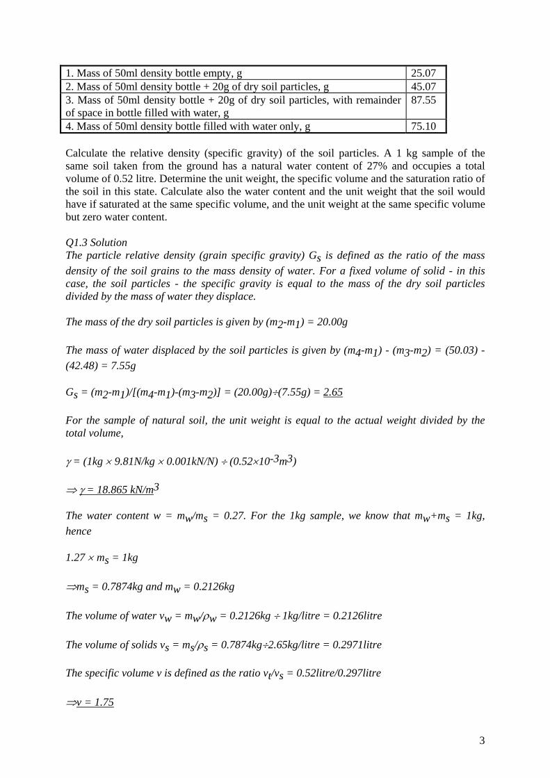
1. Mass of 50ml density bottle empty, g 25.07 2. Mass of 50ml density bottle + 20g of dry soil particles, g 45.07 3. Mass of 50ml density bottle + 20g of dry soil particles, with remainder of space in bottle filled with water, g
87.55
4. Mass of 50ml density bottle filled with water only, g 75.10 Calculate the relative density (specific gravity) of the soil particles. A 1 kg sample of the same soil taken from the ground has a natural water content of 27% and occupies a total volume of 0.52 litre. Determine the unit weight, the specific volume and the saturation ratio of the soil in this state. Calculate also the water content and the unit weight that the soil would have if saturated at the same specific volume, and the unit weight at the same specific volume but zero water content. Q1.3 Solution The particle relative density (grain specific gravity) Gs is defined as the ratio of the mass density of the soil grains to the mass density of water. For a fixed volume of solid - in this case, the soil particles - the specific gravity is equal to the mass of the dry soil particles divided by the mass of water they displace. The mass of the dry soil particles is given by (m2-m1) = 20.00g The mass of water displaced by the soil particles is given by (m4-m1) - (m3-m2) = (50.03) - (42.48) = 7.55g Gs = (m2-m1)/[(m4-m1)-(m3-m2)] = (20.00g)÷(7.55g) = 2.65 For the sample of natural soil, the unit weight is equal to the actual weight divided by the total volume, γ = (1kg × 9.81N/kg × 0.001kN/N) ÷ (0.52×10⁻³m3) ⇒ γ = 18.865 kN/m3 The water content w = mw/ms = 0.27. For the 1kg sample, we know that mw+ms = 1kg, hence 1.27 × ms = 1kg ⇒ms = 0.7874kg and mw = 0.2126kg The volume of water vw = mw/ρw = 0.2126kg ÷ 1kg/litre = 0.2126litre The volume of solids vs = ms/ρs = 0.7874kg÷2.65kg/litre = 0.2971litre The specific volume v is defined as the ratio vt/vs = 0.52litre/0.297litre ⇒v = 1.75

4
The saturation ratio is given by the volume of water divided by the total void volume, = 0.2126litre ÷(0.52litre - 0.297litre) = 0.9534 ⇒Sr = 95.34% If the soil were fully saturated, the volume of water would be (0.52litre - 0.297litre) = 0.223litre. The mass of water would be 0.223kg, and the water content would be 0.223kg ÷ 0.7874kg ⇒wsat = 28.32% The overall mass of the 0.52litre sample would be 0.223kg + 0.7874kg = 1.0104kg, and its unit weight (1.0101kg × 9.81N/kg × 10-3kN/N) ÷ (0.52×10⁻³m3) ⇒γsat = 19.06kN/m3 If the soil were dry but had the same specific (and overall) volume, the mass would be equal to the mass of solids alone, and the unit weight would be (0.7874kg × 9.81N/kg ×10-3kN/N) ÷ (0.52×10⁻³m3) ⇒γdry = 14.86 kN/m3 Q1.4 An office block with an adjacent underground car park is to be built at a site where a 6m-thick layer of saturated clay (γ = 20 kN/m3) is overlain by 4m of sands and gravels (γ = 18 kN/m3). The water table is at the top of the clay layer, and pore water pressures are hydrostatic below this depth. The foundation for the office block will exert a uniform surcharge of 90 kPa at the surface of the sands and gravels. The foundation for the car park will exert a surcharge of 40 kPa at the surface of the clay, following removal by excavation of the sands and gravels. Calculate the initial and final vertical total stress, pore water pressure and vertical effective stress, at the mid-depth of the clay layer, (a) beneath the office block; and (b) beneath the car park. Take the unit weight of water as 9.81kN/m3. Q1.4 Solution Initially, the stress state is the same at both locations. The vertical total stressσv = (4m ×
18kN/m3) (for the sands and gravels) + (3m × 20kN/m3) (for the clay), giving σv = 132 kPa The pore water pressure u = (3m × 9.81kN/m3) = 29.4 kPa The vertical effective stress σ'v = σv - u = (132kPa - 29.4kPa) = 102.6 kPa Finally,

5
(a) Beneath the office block, the vertical total stress is increased by the surcharge of 90kPa, giving σv = 132kPa + 90 kPa ⇒ σv = 222 kPa The pore water pressure u is unchanged, ⇒ u = 29.4kPa The vertical effective stress σ'v = σv - u = (222kPa - 29.4kPa) ⇒σ'v = 192.6 kPa (b) Beneath the car park, the vertical total stress is given by σv = (40kPa) (surcharge) + (3m × 20kPa) (for the clay) ⇒ σv = 100 kPa The pore water pressure u is unchanged, ⇒ u = 29.4kPa The vertical effective stress σ'v = σv - u = (100kPa - 29.4kPa) ⇒σ'v = 70.6 kPa Q1.5 For the measuring cylinder experiment described in main text Example 1.3, calculate (a) the vertical effective stress at the base of the column of sand in its loose, dry state; (b) the pore water pressure and vertical effective stress at the base of the column in its loose, saturated state; (c) the pore water pressure and vertical effective stress at the base of the column in its dense, saturated state; and (d) the pore water pressure and vertical effective stress at the sand surface in the dense, saturated state. Take the unit weight of water as 9.81kN/m3. Q1.5 Solution (a) In the loose dry state, the vertical total stress is given by the unit weight of the sand × the depth h. The depth of the sand is given by the volume, 1200cm3, divided by the cross-sectional area of the measuring cylinder, 28.27cm2, giving h = 42.448cm. Henceσv =
16.35kN/m3 × 0.4245m = 6.94kPa. As the sand is dry, the pore water pressure u = 0 and σ'v = σv = 6.94kPa (Alternatively, the total weight of sand is 2kg × 9.81×10-3kN/kg = 0.01962kN. This is spread over an area of (π × 0.062m2) ÷ 4 = 0.002827m2. Hence the total stressσv = 0.01962kN ÷
0.002827m2 = 6.94 kPa.) (b) In the loose, saturated state, the pore water pressure u = 0.4245m × 9.81kN/m3 ⇒u = 4.164 kPa

6
The vertical total stress σv = 19.99kN/m3 × 0.4245m = 8.486kPa. Hence the vertical effective stress σ'v = σv - u = 8.486kPa - 4.164kPa ⇒ σ'v = 4.322kPa (c) In the dense, saturated state, the weights of water and soil grains above the base do not change. Hence the pore water pressure and the total stress are the same as before, and so also is the effective stress: u = 4.164 kPa; σ'v = 4.322kPa (d) The water level in the column does not change: as the sand is densified, it settles through the water. The new sample height h' is given by its volume, 1130cm3, divided by the cross-sectional area of the measuring cylinder, 28.27cm2, giving h' = 39.972cm. The depth of water above the new sample surface is therefore (42.448cm - 39.972cm) = 2.476cm. The pore water pressure at the new soil surface is 9.81kN/m3 × 0.02476m ⇒ u = 0.243kPa The effective stress at the sand surface is zero. Particle size analysis and soil filters Q1.6 A sieve analysis on a sample of initial total mass 294g gave the following results: Sieve size, mm 6.3 3.3 2.0 1.2 0.6 0.3 0.15 0.063 Mass retained, g 0 0 30 39 28 28 16 11 A sedimentation test on the 117 g of soil collected in the pan at the base of the sieve stack gave: Size, µm <2 2-6 6-15 15-30 30-63 % of pan sample 0 48 29 14 9 Plot the particle size distribution curve and classify the soil using the system given in Table 1.5. Determine the D10 particle size and the uniformity coefficient U, and comment on the grading curve. Q1.6 Solution First, note that the total of the masses retained is 152g, which together with the 117g collected in the pan gives 269g. Thus there is a shortfall of 25g, which is presumably attributable to sieve losses. Take the total mass of the sample as 269g. The % by mass of the sample passing each sieve is given by the total sample mass (269g) minus the cumulative mass of soil retained on larger size sieves. Hence

7
Sieve size, mm 6.3 3.3 2.0 1.2 0.6 0.3 0.15 0.063 Mass retained, g 0 0 30 39 28 28 16 11 Cumulative mass retained, g
0 0 30 69 97 125 141 152
Mass passing, g 269 269 239 200 172 144 128 117 % passing 100 100 88.8 74.3 63.9 53.5 47.6 43.5 The sedimentation test data are already part-processed, with the mass of soil in each size range expressed as a percentage of the 117g collected in the pan. This is slightly different from main text Example 1.5, in which raw data are given. The fraction of the pan sample smaller than a given size is given by 100% minus the cumulative percentage in the larger size ranges. To convert this to a percentage of the total sample, we must multiply by 117g and divide by 269g. Hence Size, µm <2 2-6 6-15 15-30 30-63 % of pan sample 0 48 29 14 9 Size, µm 2 6 15 30 63 % of pan sample smaller than this size
(48-48) = 0
(77-29) = 48
(91-14) = 77
(100-9) = 91
100
% of total sample smaller than this size
0 20.9 33.5 39.6 43.5
The particle size distribution curve is plotted in Figure Q1.6, using the data shown in bold type.
Figure Q1.6: Particle size distribution curve

8
Reading off from the curve, D10 ≈ 0.0035 mm (3.5µm) D60 ≈ 0.52 mm Hence the uniformity coefficient U = D60/D10 ≈ 150 (148.6) The soil is approximately 40% silt, 50% sand and 10% fine gravel: this makes it a sandy SILT according to the system given in Table 1.5. The soil is poorly (almost gap-) graded. Q1.7 A sieve analysis on a sample of initial total mass 411g gave the following results: Sieve size, mm 6.3 1.2 0.3 0.063 Mass retained, g 0 60 126 92 A sedimentation test on the 121 g of soil collected in the pan at the base of the sieve stack gave: Size, µm <2 2-10 10-60 % of pan sample 33 24 43 Plot the particle size distribution curve and classify the soil using the system given in Table 1.5. On the PSD diagram, sketch a suitable curve for a granular filter to be used between this soil and a drainage pipe with 3 mm perforations. Q1.7 Solution The total of the masses retained is 278g, which together with the 121g collected in the pan gives 399g. Thus there is a shortfall of 12g, which is attributable to sieve losses. Take the total mass of the sample as 399g. The % by mass of the sample passing each sieve is given by the total sample mass (399g) minus the cumulative mass of soil retained on larger size sieves. Hence Sieve size, mm 6.3 1.2 0.3 0.063 Mass retained, g 0 60 126 92 Cumulative mass retained, g
0 60 186 278
Mass passing, g 399 339 213 121 % passing 100 85.0 53.4 30.3 The sedimentation test data are again already part-processed, with the mass of soil in each size range expressed as a percentage of the 121g collected in the pan. The fraction of the pan sample smaller than a given size is equal to the sum of the percentages in this and the smaller

9
size ranges. To convert this to a percentage of the total sample, we must multiply by 121g and divide by 399g. Hence Size, µm <2 2-10 10-60 % of pan sample 33 24 43 Size, µm 2 10 60 % of pan sample smaller than this size
33 (33+24) = 57
(33+24+43)=100
% of total sample smaller than this size
10.0 17.3 33.0
The particle size distribution curve is plotted in Figure Q1.7 using the data shown in bold type. Reading from the PSD curve, the soil is approximately 10% clay, 20% silt, 60% sand and 10% fine gravel: this makes it a clayey, very silty SAND. Also reading from the curve, D15s≈0.007 mm, D85s≈1.2 mm Q1.7 SOLUTION The filter PSD curve is sketched on Figure Q1.7 according to the following rules.
• D15f ≤ 5 × D85s (main text Equation 1.18) ⇒ D15f ≤ 6 mm (point B on Figure Q1.7) • D15f > 4 × D15s (main text Equation 1.19) ⇒ D15f > 0.028 mm (point A on Figure
Q1.7) • D5f ≥ 63 µm (main text Equation 1.18; point C on Figure Q1.7) • D10f ~ slot width = 3 mm (point D on Figure Q1.7) • D60f ≤ ~3 × D10f (main text Equation 1.21) ⇒ D60f ≤ ~9 mm (point E on Figure Q1.7)
Using a degree of judgement to account for the very wide range of particle size present in the natural soil, and recalling the advice given by Preene et al (2000) that in variable ground main text Equation 1.18 should be applied to the finest soil and main text Equation 1.19 to the coarsest, a suitable PSD curve for the filter is sketched in Figure Q1.7.

10
0
10
20
30
40
50
60
70
80
90
100
0.001 0.01 0.1 1 10 100
Particle size (mm)
Perc
enta
ge p
assi
ng
GRAVELSANDSILT
CoarseMediumFineCoarseMediumFineCoarseMediumFineCLAY
Filter PSDSoil PSD
C
E
D
A B
Figure Q1.7: Particle size distribution curves for natural soil and suitable filter Index tests and classification Q1.8 The following results were obtained from a series of cone penetrometer tests using a standard 80g, 30° cone. Mass of tin empty, g
18.2 19.1 17.7 18.6
Mass of tin + sample wet, g
51.5 45.5 50.7 43.4
Mass of tin + sample dry, g
37.8 35.6 39.7 36.3
Cone penetration d, mm
25.0 14.2 8.5 5.1
Determine the water content w of each sample. Plot a graph of w against ln(d), and estimate the liquid limit wLL. If the soil has a plastic limit of 22%, calculate the plasticity index and classify the soil using the chart given in Figure 1.15. Q1.8 Solution The water content is the mass of water divided by the mass of soil solids, i.e. {(ms+mw+mt) - (ms+mt)} ÷ {(ms+mt) - (mt)}:

11
Mass of tin empty, g (mt)
18.2 19.1 17.7 18.6
Mass of tin + sample wet, g (ms+mw+mt)
51.5 45.5 50.7 43.4
Mass of tin + sample dry, g (ms+mt)
37.8 35.6 39.7 36.3
ms/mw, % 69.9 60.0 50.0 40.1 Cone penetration d, mm
25.0 14.2 8.5 5.1
ln(d) 3.219 2.653 2.14 1.63 A graph of w against ln(d) is plotted in Figure Q1.8. The liquid limit corresponds to a cone penetration of 20mm, i.e. ln(d) = 2.996. Reading from the graph, wLL≈65% The plasticity index PI = wLL - wPL = 65% - 22% ⇒ PI≈43%. By plotting the point wLL=65%; PI=43% on the chart given in main text Figure 1.15, the soil can be classified as a high plasticity clay (CH).
Figure Q1.8: water content against ln(cone penetration)

12
Compaction Q1.9 The following results were obtained from a standard (2.5 kg) Proctor compaction test: Mass of tin empty, g 14 14 14 14 14 Mass of tin + sample wet, g 88 68 98 94 93 Mass of tin + sample dry, g 81 62 87 82 80 Density, kg/m3 1730 1950 2020 1930 1860 Plot a graph to determine (i) the maximum dry density, (ii) the optimum water content and (iii) the actual density at the optimum water content. If the particle relative density (grain specific gravity) Gs = 2.65, calculate (iv) the specific volume and (v) the saturation ratio at the maximum dry density. Q1.9 Solution We need to plot a graph of water content w against dry density ρdry, where w = mw/ms (main text Equation 1.5) and ρdry = ρ/(1+w) (main text Equation 1.27) The water content of each sample is calculated as in Example E1.1: ( ) ( ){ }
( ){ })( tmsmtmsmtmwmsmtm
smwm
w−+
+−++==
where (mt) = mass of tin, empty (mt + ms + mw) = mass of tin + wet soil sample (mt +ms) = mass of tin + dry soil sample

13
Hence Mass of tin empty, g 14 14 14 14 14 Mass of tin + sample wet, g 88 68 98 94 93 Mass of tin + sample dry, g 81 62 87 82 80 w, % 10.45 12.5 15.07 17.65 19.70 Density, kg/m3 1730 1950 2020 1930 1860
Dry density, kg/m3 1566 1733 1755 1640 1554
Figure Q1.9: dry density against water content From the graph (Figure Q1.9), • the maximum dry density ρdry,max ≈ 1770 kg/m3
• the optimum water content (at ρdry,max ) ≈ 14% • the actual density at the optimum water content = 1770 kg/m3 × 1.14 = 2018 kg/m3 The specific volume v can be calculated using main text Equation 1.8, γ = [Gs.(1+w)/v].γw (main text Equation 1.8) or v = Gs.(1+w).(γw/γ)

14
hence v = 2.65 × (1.14) × (1000/2018) = 1.497 (The void ratio e = v-1 = 0.497) The saturation ratio Sr is calculated using main text Equation 1.10, Sr = w.Gs/e = w.Gs/(v-1) (main text Equation 1.10) Sr = 0.14 × 2.65 ÷ 0.497 = 0.746 or 74.6%

15
QUESTIONS AND SOLUTIONS: CHAPTER 2 The shearbox test Q2.1 Describe with the aid of a diagram the essential features of the conventional shearbox apparatus. Stating clearly the assumptions you need to make, show how the quantities measured during the test are related to the stresses and strains in the soil sample. [University of London 2nd year BEng (Civil Engineering) examination, King's College (part question)] Q2.1 Solution Diagram of shear box: See main text Figure 2.14 Assume that the stresses and strains are uniform and continuous, and that the actual deformation in shear (main text Figure 2.15a) is idealised as indicated in main text Figure 2.15b. The known or measured quantities are A the sample area on plan, assumed to remain constant during the test) H the initial height of the sample N the normal (hanger) load F the shear force x the relative horizontal displacement between the upper and lower halves of the
shearbox y the upward movement of the shearbox lid. Consideration of main text Figure 2.15b gives strains shear strain γ = x/H volumetric strain εvol = -y/H In terms of stresses, shear stress on central horizontal plane τ = F/A normal stress on central horizontal plane σ = N/A If it is further assumed that the pore water pressure u is zero (so that σ' = σ) and the central horizontal plane is the plane of maximum stress obliquity (τ/σ')max, a Mohr circle of stress may be drawn (eg main text Figure 2.30), and the mobilised effective angle of friction is φ'mob = tan-1{(τ/σ')max} Q2.2 With the aid of sketches, describe, explain and contrast the results you would expect to obtain from conventional shearbox tests on samples of dry sand which were (a) initially loose, and (b) initially dense. What factors would you take into account in selecting a soil strength parameter for use in design? [University of London 2nd year BEng (Civil Engineering) examination, King's College (part question)]
16
Q2.2 Solution Typical graphs of (a) shear stress τ against shear strain γ; (b) volumetric strain εvol against shear strain γ ; and (c) specific volume v against shear strain γ are as shown in main text Figure 2.21. In the test carried out on the initially dense sample, the shear stress gradually increases with shear strain to a peak at P, before falling to a steady value at C which is maintained as the shear strain is increased. The sample may undergo a very small compression at the start of shear, but then begins to dilate. The curve of ε vol vs γ becomes steeper, indicating that the rate of dilation -dεvol/dγ is increasing. The slope of the curve reaches a maximum at p, but with continued shear strain the curve becomes less steep until at c it is horizontal. When the curve is horizontal dεvol/dγ is zero, indicating that dilation has ceased. The peak shear stress at P coincides with the maximum rate of dilation at p. The steady state shear stress at C corresponds to the achievement of the critical specific volume at c. The initially loose sample displays no peak strength, but eventually reaches the same critical shear stress as the first sample. The second sample does not dilate, but gradually compresses during shear until the same critical specific volume is reached (i.e. the volumetric strain remains constant). In both cases, a critical state, is reached in which the soil continues to shear at constant specific volume, constant shear stress and constant normal effective stress. A dense sample displays a peak strength because additional work has to be done to overcome the effect of the initially high degree of interlocking – high, that is, relative to the equilibrium specific volume for continued shear at the vertical effective stress at which the test is carried out. The initial dense packing means that the particles are forced to “ride up” over each other (⇒ dilation) for deformation to occur (see the “saw blades analogy”, Figure 2.24). In design, it may be safer to use the critical state strength φ'crit than the peak strength φ'peak, because
• the peak strength depends on the extent to which the soil is dense in relation to the critical state under the effective stress conditions at failure. It is not a soil constant, and is unlikely to be the same throughout the mass of soil involved in a potential failure mechanism
• it is unlikely that the peak strength will be mobilised simultaneously throughout the soil mass; instead, progressive failure at an average strength rather lower than the peak may occur.
However, the factors of safety used in many traditional methods of design may well allow for these possibilities, and their use in connection with the critical state strength could lead to overconservatism.

17
Development of a critical state model Q2.3 Mining operations frequently generate large quantities of fine, particulate waste known as tailings. Tailings are generally transported as slurries, and stored in reservoirs impounded by embankments or dams made up from the material itself. In order to investigate the geotechnical behaviour of a particular tailings material (Gs=2.70), an engineer carried out three slow, drained shear tests - each over a period of one day - and three fast, undrained shear tests - each over a period of two minutes - in a conventional 60mm × 60 mm shearbox apparatus. The three samples in each group were initially allowed to come into drained equilibrium under the application of vertical hanger loads of 100 N, 200 N and 300 N. During each shear test, the hanger load was kept constant and the ultimate shear force Fult recorded. Immediately after each test, a water content sample was taken from the centre of the rupture zone. All of the samples were initially saturated, and all of the tests were carried out with the sample under water in the shearbox. Use the results of the drained tests to construct a critical state model in terms of the normal effective stress σ' and shear stress τ on the shear plane, and the specific volume v. Give the values of φ'crit, vo and λ. Deduce a relationship between the undrained shear strength τu and the normal effective stress at the start of the test, and compare its predictions with the experimental data from the undrained tests. Test type Vertical load V, N Shear load Fult, N Water content w,
% slow, drained 100 53 35.1 200 105 31.3 300 156 29.5 fast, undrained 100 42 36.0 200 80 32.6 300 120 30.6 Q2.3 Solution The critical state model must be constructed using the drained test data only, because only in these tests do we know that the pore water pressure u = 0 and that the vertical effective stress σ' is equal to the normal load divided by the sample area. We must assume that the data given for the slow tests were measured at true critical states. For each sample, the normal effective stress σ' = V (kN)/A (m2) the ultimate shear stress tult = Fult (kN)/A (m2) and the specific volume v may be calculated from the water content w using main text Equation 1.10 with Sr=1, v = 1 + w.Gs (main text Equation 2.12)

18
Vertical load V, N
normal effective stress σ', kPa
ln(σ') Shear load Fult, N
Shear stress τult, kPa
Water content w, %
Specific volume v
100 27.8 3.325 53 14.7 35.1 1.95 200 55.6 4.018 105 29.2 31.3 1.85 300 83.3 4.422 156 43.3 29.5 1.80 Plot graphs of τult against σ' and v against lnσ' to determine the critical state parameters, as in main text Figure 2.28 (Example 2.2). φ'crit ≈ 28°; vo ≈ 2.43; λ ≈ 0.14 During the undrained tests, there is no overall volume change. Assuming that the specific volume is uniform throughout the sample, it must remain constant during the test. The critical state eventually reached therefore depends on the as-tested specific volume. Our model predicts that, at the critical state, the vertical effective stress σ' is related to the specific volume by the expression v = vo - λ.lnσ' (main text Equation 2.11) or σ' = exp{(vo-v)/λ} The normal effective stress at the critical state is related to the shear stress τult by the expression τult = σ'.tanφ'crit (main text Equation 2.10) Hence τult = exp{(vo-v)/λ}.tanφ'crit where v = 1 + w.Gs. The calculated and measured values of τult for the undrained tests are compared below: Vertical load V, N
normal effective stress σ', kPa
Shear load Fult, N
Measured shear stress τult, kPa
Water content w, %
Specific volume v
Calculated shear stress, τult kPa
100 27.8 42 11.7 36.0 1.972 14.0 200 55.6 80 22.2 32.6 1.880 27.0 300 83.3 120 33.3 20.6 1.826 39.8 The measured values are smaller than the theoretical values by about 16%. This is probably due to internal drainage and discontinuous sample behaviour.

19
Determination of peak strengths Q2.4 The following results were obtained from a shearbox test on a 60 mm × 60 mm sample of dry sand of unit weight 18 kN/m3. Reading on proving ring deflexion
dial gauge (divisions) Zero force 91 Peak shear force for a hanger load of 3kg 128 Peak shear force for a hanger load of 10kg 162 Peak shear force for a hanger load of 20kg 210 One division on the proving ring dial gauge corresponds to a force of 1.1N across the proving ring. (a) Plot the data on a graph of shear stress against normal effective stress, and sketch the peak strength failure envelope. (b) What is the peak resistance to shear on a horizontal plane at a depth of 3 m below the top of a dry embankment made from this soil? (c) A model of the embankment is constructed from the same sand at a scale of 1:10. What is the peak resistance to shear on a horizontal plane at a depth of 300mm below the top of the model? (d) Would you expect the model to behave in the same way as the real embankment? Q2.4 Solution (a) The normal stress on the sample is given by the hanger load (kg) × 9.81 (N/kg) ÷ the sample area, 0.06m × 0.06m = 3.6×10⁻³m2, ÷ 1000 to convert from Pa to kPa. The shear force on the sample is given by 1.1 × (the number of proving ring dial divisions - the number of divisions at zero load), i.e. 1.1 × (n - 91). To convert this to the shear stress, it is necessary to divide the shear force by the area of the sample, 0.06m × 0.06m = 3.6×10⁻³m2, and divide by 1000 to convert from Pa to kPa. Hanger load, kg Normal stress, kPa Peak shear load, N Peak shear stress, kPa 3 8.175 40.7 11.31 10 27.25 78.1 21.69 20 54.5 130.9 36.36 These data are plotted on a graph of τ against σ' in Figure Q2.4. The peak strength failure envelope is highly non-linear, with φ'peak = 55° at σ' ≈ 8 kPa, falling to φ'peak = 34° at σ' ≈ 55 kPa

20
(b) At a depth of 3m below the top of a dry embankment made of this sand, the vertical effective stress is 3m×18kN/m3 = 54kPa. This corresponds to a hanger load of 20kg, at which the peak shear stress is approximately 36.4 kPa (c) In the 1:10 scale model, the vertical effective stress at a depth of 300mm is about 0.3m × 18kN/m3 = 5.4 kPa. From Figure Q2.4, this gives a peak shear resistance of approximately 7.7kPa (d) The model would not be expected to behave in the same way as the real embankment, because the operational values of φ'peak at corresponding depths in the model and the real embankment are quite different.
Figure Q2.4: Shear stress against normal effective stress at peak

21
Use of strength data to calculate friction pile load capacity Q2.5 A friction pile, 300 mm in diameter, is driven to a depth of 25 m in dense sand of unit weight 19 kN/m3. The ratio of horizontal to vertical effective stresses is 0.5. The angle of friction between the pile and the sand is 26° and the resistance offered at the base of the pile may be ignored. The natural water table, below which the pore water pressures are hydrostatic, is 5m below ground level. During construction works, the water table is temporarily lowered to a depth of 16m by pumping from wells. A load test on the pile is carried out while pumping to lower the groundwater level is still in progress. Calculate the ultimate load capacity of the pile (a) observed in the test, and (b) after pumping from the wells has stopped, and the water table has recovered to its natural level. Q2.5 Solution The vertical total stress σv, the pore water pressure u and the vertical (σ'v) and horizontal (σ'h) effective stresses all vary linearly with depth between the soil surface and the water table, and between the water table and the base of the pile. In general at depth z, with the water table at a depth h, σv = γ.z; u = 0 above the water table (z≤h) u = γw.(z - h) below the water table (z≥h) σ'v = σv - u σ'h = 0.5 × σ'v shear stress on pile τ = σ'h ×tan26° (a) With the water table depth h = 16m. γ = 19 kN/m3 and γw = 9.81 kN/m3, the following relationship between shear stress τ and depth z is calculated: z, m σv, kPa u, kPa σ'v, kPa σ'h, kPa τ, kPa At the soil surface 0 0 0 0 0 0 At the water table 16 304 0 304 152 74.14 At the base of the pile 25 475 88.29 386.71 193.36 94.31 The frictional resistance to pile movement is given by integrating the shear stress τ over the surface area of the pile. The surface area of the upper 16m of the pile is (π × 0.3)m × 16m = 15.08m2, and the average shear stress over this area is 74.14kPa ÷ 2 = 37.07kPa. The surface area of the lower 9m of the pile is (π × 0.3)m × 9m = 8.48m2, and the average shear stress over this area is (74.14kPa + 94.31kPa) ÷ 2 = 84.23kPa. Thus the overall frictional resistance is (15.08m2 × 37.07kPa) + (8.48m2 × 84.23kPa) = 1273kN (b) With the water table depth h = 5m. γ = 19 kN/m3 and γw = 9.81 kN/m3:

22
z, m σv, kPa u, kPa σ'v, kPa σ'h, kPa τ, kPa At the soil surface 0 0 0 0 0 0 At the water table 5 95 0 95 47.5 23.17 At the base of the pile 25 475 196.2 278.8 139.4 67.99 The surface area of the upper 5m of the pile is (π × 0.3)m × 5m = 4.71m2, and the average shear stress over this area is 23.17kPa ÷ 2 = 11.59kPa. The surface area of the lower 20m of the pile is (π × 0.3)m × 9m = 18.85m2, and the average shear stress over this area is (23.17kPa + 67.99kPa) ÷ 2 = 45.58kPa. Thus the overall frictional resistance is (4.71m2 × 11.59kPa) + (18.85m2 × 45.58kPa) = 914kN Q2.6 The depth of the friction uplift pile described in main text Example 2.4 is increased to 20m, where the undrained shear strength of the clay is 40 kPa. Calculate the short- and long-term uplift resistance of the 20m pile. Q2.6 Solution The total shear resistance of the clay/pile interface is given by T = average shear stress × surface area of pile (a) In the short term, the average shear stress is the average undrained shear strength on the interface, so that T = [(0 + 40kPa) ÷ 2] × [(π × 0.5m) × 20m] = 628 kN (b) In the long term, the ultimate shear stress on the interface is given by τult = σ'h.tanδ where σ'h = 0.5 × σ'v is the horizontal effective stress and δ is the angle of friction between the clay and the pile At a depth z, σv (kPa) = {γ (kN/m3) × z (m)} = {18 (kN/m3) × z (m)} u (kPa) = {γw (kN/m3) × z (m)} = {9.81 (kN/m3) × z (m)}, and σ'v = σv - u As in (a), T = average shear stress × surface area of pile The shear stress τ on the soil/pile interface is now

23
0.5 × σ'v.tanδ which increases linearly from zero at the top of the pile to 0.5 × [(18 kN/m3 × 20 m) - (9.81 kN/m3 × 20 m)] × tan20° = 29.81 kPa at the base Hence T = [(0 + 29.81 kPa) ÷ 2] × [(π × 0.5 m) × 20 m] = 468 kN Stress analysis and interpretation of shearbox test data Q2.7 A drained shearbox test was carried out on a sample of saturated sand. The normal effective stress of 41.67 kPa was constant throughout the test, and the initial sample dimensions were 60 mm × 60 mm on plan × 30 mm deep). In the vicinity of the peak shear stress, the data recorded were: Shear stress τ, kPa 42.5 43.1 42.8 relative horizontal displacement x, mm 0.30 0.40 0.80 upward movement of shearbox lid y, mm 0.05 0.075 0.105 (a) Draw the Mohr circle of stress for the soil sample when the shear stress is a maximum, stating the assumption that you need to make. Determine φ'peak, and the orientations of the planes of maximum stress ratio (τ/σ')max. Draw the Mohr circle of strain increment leading to the peak, and hence determine the maximum angle of dilation, ψmax. Use an empirical relationship between φ'peak,ψmax and φ'crit to estimate the critical state friction angle, φ'crit. (b) Three further drained tests on similar samples of the same soil were carried out, at different normal effective stresses. The peak and critical state shear stresses were: Normal effective stress, kPa 20 100 200 Peak shear stress, kPa 23.8 83.9 132.0 Critical state shear stress, kPa 12.6 63.2 126.4 For all four tests, plot the peak and critical state shear stresses τpeak and τcrit as a function of the normal effective stress σ'. Sketch failure envelopes for both peak and critical states, and comment briefly on their shapes. Which would you use for design, and why? [University of London 2nd year BEng (Civil Engineering) examination, King's College (part question)] Q2.7 Solution (a) At τmax (= 43.1 kPa), φ'peak = tan-1{(τ/σ')max} = tan-1(43.1/41.67) = 46° assuming that the central horizontal plane is a plane of maximum stress ratio. The Mohr circle of stress is shown in Figure Q2.7a.

24
46° 90° - 46°
40
20
60
0100 σ’ kN/m2
τ kN/m2
Figure Q2.7a: Mohr circle of stress The first plane of maximum stress ratio is horizontal (this is an assumption that has to be made to draw the Mohr circle of stress). From Figure Q2.7a, the second plane of maximum stress ratio is at (90° - φ'peak) = (90° - 46°) = 44° to the horizontal, either clockwise or anticlockwise depending on whether the shear stress on the horizontal plane plots positive or negative. (Note: the answer given in the main text is slightly ambiguous here. The planes of maximum stress ratio are horizontal and either + or - 44° to the horizontal and not, as might be interpreted from the answer given in the main text, + and - 44° to the horizontal). The increments of shear (∆γ) and vertical (∆εv) strain leading up to peak are given by ∆εv = ∆y/H = 0.025/30 = 0.083%, and ∆γ = ∆x/H = 0.1/30 = 0.333% where ∆x and ∆y are the incremental relative horizontal displacement of the two halves of the shearbox and the upward displacement of the shearbox lid respectively, and H = 30 mm ins the initial sample height. The increment of horizontal strain ∆εh = 0. The Mohr circle of strain increment is shown in Figure Q2.7b, and is plotted with coordinates (∆ε, ∆γ/2) = (0.083%, 0.167%) for the strains associated with (normal to) the horizontal plane and (0, -0.167%) for the strains associated with (normal to) the vertical plane.

25
0.083
0.167
Ψmax = 14°
∆γ/2 %
∆ε %
V
H
Figure Q2.7b: Mohr circle of strain increment leading up to peak From Figure Q2.7b, the angle of dilation at peak is given by ψmax = ∆y/∆x = 2.5/10 ⇒ ψmax = 14° We might expect φ'crit ~ φ'peak – 0.8 × ψmax (main text Equation 2.14), giving φ'crit ~ 46° - 11° or φ'crit ~35° (b) The data are plotted as τpeak and τcrit against σ' in Figure Q2.7c.
Figure Q2.7c: Failure envelopes in terms of peak and critical state strengths
26
The failure envelopes sketched in Figure Q2.7c show that
• φ'crit is constant (= 32.5°, closer to φ'peak –ψmax = 32° than the estimate of 35° based on φ'peak – 0.8 × ψmax) because there is no dilation at the critical state
• φ'peak reduces as the normal effective stress σ' increases, because the amount of dilation needed to reach the appropriate (critical) specific volume is reduced.
In design, it may be safer to use the critical state strength φ'crit than the peak strength φ'peak, because
• the peak strength depends on the extent to which the soil is dense in relation to the critical state under the effective stress conditions at failure. It is not a soil constant, and is unlikely to be the same throughout the mass of soil involved in a potential failure mechanism
• it is unlikely that the peak strength will be mobilised simultaneously throughout the soil mass; instead, progressive failure at an average strength rather lower than the peak may occur.
However, the factors of safety used in may traditional methods of design may well allow for these possibilities, and their use in connection with the critical state strength could lead to overconservative design. Q2.8 In order to investigate the drained strength of a natural silt containing thin clay laminations at a spacing of approximately 6 mm, an engineer carried out a series of shearbox tests. The clay laminations were inclined at various angles θ to the horizontal. With the laminations horizontal (θ = 0), the rupture formed entirely in the clay and the apparent angle of shearing resistance was 18°. With the laminations at an angle θ = 60°, the rupture formed entirely in the silt and the apparent angle of shearing resistance was 30°. Stating clearly the assumptions you need to make, construct Mohr circles of stress at failure for various values of apparent angle of shearing resistance, marking on each the stress state corresponding to the clay laminations. (Hint: the mobilized strength on the clay laminations must never exceed 18°). Plot a graph showing the relationship between the angle θ and the apparent angle of shearing resistance of the soil. [University of London 1st year BEng (Civil Engineering) examination, King's College (part question)] Q2.8Solution When θ = 0, the shear plane forms in the clay so φ'crit = 18° for the clay. When θ = 60°, the shear plane forms in the silt so φ'crit = 30° for the silt. Assume that the sample behaves as a continuum up to rupture, and that the central horizontal plane of the shearbox is the plane of maximum and apparent stress ratio (τ/σ') = tanφ'apparent. The easiest procedure is to construct Mohr circles of stress for apparent φ' values of 21°, 24°, 27° and 30° and deduce the corresponding orientation of the clay laminations such that the stress ratio on the laminations is (τ/σ') = tan18° . Each value of φ'apparent will give four possible orientations of the clay laminations (θ measured clockwise from the horizontal), as indicated in Figure Q2.8a. Figure Q2.8a shows a general Mohr circle from which algebraic expressions for the orientations θ (measured clockwise from the horizontal) of the yellow clay laminations to give

27
the given value of φ'apparent. Remember that the rotation on the Mohr circle must be divided by 2 to give the actual rotation in the physical plane.
2θ1
ω1
C
90° + φ’apparent90° - φ’apparent
ω4
PT
O
S
Q
R
18°
φ’apparent
φ’apparent
φ’ = 18°
s’
t
σ’
τ
Figure Q2.8a: Mohr circle of stress The orientations θ of the clay laminations are given by the angles clockwise from the horizontal plane θ1, θ2, θ3 and θ4, corresponding to the points P, Q, R and S respectively on Figure Q2.8a. From triangle OTC, t/s' = sinφ'apparent From triangle OPC, angle OCP = 180° - ω1 - 18° and angle OCP = 2θ1 + (90° - φ'apparent) Applying the sine rule to triangle OPC, s'/sinω1 = t/sin18° ⇒ sinω1 = sin18°/(t/s') or sinω1 = sin18°/sinφ'apparent (note ω1 is acute, ie less than 90°) Applying the sine rule to triangle OSC, s'/sinω4 = t/sin18° ⇒ sinω4 = sin18°/(t/s') or sinω4 = sin18°/sinφ'apparent (note ω4 is obtuse, ie greater than 90°) By considering the geometry of the Mohr circle shown in Figure Q2.8a, the values of θ1 to θ4 may be determined as follows. 2θ1 = (90° + φ'apparent) - (ω1 + 18° ) ⇒ θ1 = 0.5 × (72° - ω1 + φ'apparent)

28
2θ2 = (90° + φ'apparent) + (ω1 + 18° ) ⇒ θ2 = 0.5 × (108° + ω1 + φ'apparent) 2θ3 = (90° + φ'apparent) + (ω4 + 18° ) ⇒ θ3 = 0.5 × (108° + ω4 + φ'apparent) 2θ4 = (90° + φ'apparent) + (ω4 + 18° ) + 2(180° - 18° - ω4) ⇒ θ4 = 0.5 × (432° - ω4 + φ'apparent) The values of ω1, ω4 and θ1 to θ4 forφ'apparent = 21°, 24°, 27° and 30° are detailed in the table below. φ'apparent ω1 ω4 θ1 θ2 θ3 θ4 21 59.57 120.43 16.72 94.29 124.72 166.2824 49.44 130.56 23.28 90.72 131.28 162.7227 42.90 137.10 28.05 88.98 136.05 160.9530 38.12 141.83 31.94 88.06 139.92 160.01 These values are used to construct the graph of apparent angle of shearing resistance φ'apparent against orientation of the clay laminations θ shown in Figure Q2.8b: note that for orientations of the laminations θ between 32° and 88°, and between 140° and 160°, the value of φ'apparent is equal to φ' for the silt, 30°.
Figure Q2.8b: apparent effective angle of friction against angle of lamination inclination Note that unless you are very confident with geometry and trigonometry, this problem is probably much more easily addressed by drawing out the four individual Mohr circles to scale and measuring off the angles θ1 to θ4. The principles, and hopefully the answers, are however the same.

29
QUESTIONS AND SOLUTIONS: CHAPTER 3 Laboratory measurement of permeability; fluidization; layered soils Q3.1 Describe by means of an annotated diagram the principal features of a constant head permeameter. Give three reasons why this laboratory test might not lead to an accurate determination of the effective permeability of a large volume of soil in the ground. Suggest how each of these problems might be overcome. [University of London 2nd year BEng (Civil Engineering) examination, Queen Mary and Westfield College (part question)] Q3.1 Solution Diagram of constant head permeameter: see main text Figure 3.8 Inaccurate determination of the in situ permeability might result from
a) sample disturbance – unrepresentative void ratio of a uniform soil b) sample disturbance – destruction of soil fabric e.g. in a soil with a layered structure c) large scale inhomogeneities e.g. fissures and high permeability lenses, which cannot
be represented in the small scale laboratory sample d) low permeability of a soil with fine particles leads to inaccurate determination of
flowrate due to evaporation losses and general measurement errors These can be overcome by
a) testing recompacted samples at maximum and minimum achievable void ratio to give possible limits to the in situ permeability
b) & c) carrying out field pumping tests c) using a falling head permeameter
Q3.2 Describe by means of an annotated diagram the principal features of a falling head permeameter. Show that the water level in the top tube h would be expected to change with time t according to the following equation ln(h/ho) = -(kA1/A2L).t where ho is the initial water level in the top tube, A1 is the cross sectional area of the sample and L is its length, k is the soil permeability and A2 is the cross sectional area of the top tube. Give two reasons why this laboratory test might not lead to an accurate determination of the effective permeability of a large volume of soil in the ground. [University of London 2nd year BEng (Civil Engineering) examination, Queen Mary and Westfield College (part question)]

30
Q3.2 Solution Diagram of falling head permeameter: see main text Figure 3.10 The derivation of the equation follows the main text Section 3.4.2. At the start of the test (time t=0), the water level in the upper (small-bore) tube is at a height h0 above the permeameter outlet. After a general time t, the water level in the upper tube has fallen to a general height h above the permeameter outlet. Applying Darcy's Law at a general time t to the soil sample in the large tube, q = Aki = A1kh/L (main text Equation 3.8) In the small-bore tube, the flowrate is given by the cross-sectional area multiplied by the velocity q = A2v but the velocity v = -dh/dt so q = -A2.dh/dt (main text Equation 3.9) (the negative sign is needed because v has been taken as positive downward, while h is measured as positive upward) Equating (3.8) and (3.9) dh/dt = -(A1/A2).(k/L).h Integrating between limits of h=h0 at t=0 and the general state (h, t),
dtLk
AAhdh
h
h
t∫ ∫ ⎟⎟
⎠
⎞⎜⎜⎝
⎛−=
0 0 2
1 ./ (3.10)
hence ln(h/h0) = -(kA1/A2).(k/L).t Inaccurate determination of the in situ permeability might result from
• sample disturbance – unrepresentative void ratio of a uniform soil • sample disturbance – destruction of soil fabric e.g. in a soil with a layered structure • large scale inhomogeneities e.g. fissures and high permeability lenses, which cannot
be represented in the small scale laboratory sample • the laboratory test measures the vertical permeability, while if the field the horizontal
permeability is likely to dominate

31
Q3.3 In the constant head permeameter test described in Example E3.2, the sample was found to fluidize in upward flow at a hydraulic gradient of 0.84. Estimate the unit weight of the soil in its loosest state. [University of London 2nd year BEng (Civil Engineering) examination, Queen Mary and Westfield College (part question)] Q3.3 Solution Consider a plug of soil on the verge of uplift (main text Figure 3.24). Neglecting side friction, uplift will just occur when the upward force due to the pore water presure acting on the base (A.γw.[z+hcrit]) begins to exceed the weight of the block of soil (A.γ.z): A.γw.[z+hcrit] = A.γ.z z(γ - γw) = γw.hcrit or icrit = hcrit/z = (γ - γw)/γw (main text Equation 3.33) In the present case, icrit = 0.84. Taking γw = 9.81 kN/m3, (9.81 kN/m3 × 0.84) = g – 9.81 kN/m3 ⇒ γ = 18.05 kN/m3 (taking γw = 10 kN/m3 gives γ =18.4 kN/m3) Q3.4 An engineer wishes to investigate the bulk permeability of a layered soil comprising alternating bands of fine sand (5 mm thick) and silt (3 mm thick). The engineer makes a special constant head permeameter of square cross section (internal dimensions 112 mm × 112 mm) and carries out two tests on undisturbed samples. In one test, the flow is parallel to the laminations: in the other test, the flow is perpendicular to the laminations. The data recorded in downward flow are as follows: Hydraulic gradient i 0 1 2 5 10 Flowrate test 1, mm3/s 0 79 158 395 -
Flowrate test 2, mm3/s 0 - - 16 33 Unfortunately, the engineer is not very careful in keeping a laboratory notebook, and omits to record the orientation of the sample in each test. Estimate the permeability of the fine sand and the silt. Estimate also the flowrates at which fluidization would just occur in upward flow, both parallel and perpendicular to the laminations. Derive from first principles any formulae you use. [University of London 1st year BEng (Civil Engineering) examination, King's College (part question)]

32
Q3.4 Solution You will need to derive the formulae (main text Equations 3.21 and 3.22) for the equivalent bulk horizontal and vertical permeabilities of an alternating layer system, as in the main text Section 3.6. For horizontal flow (ie flow parallel to the laminations), the hydraulic gradient between two vertical sections A and B is the same for both layers (see main text Figure 3.16). The total flowrate qT is the sum of the flowrates through the individual layers. We seek an expression of the form qT = AT.kH.i, where kH is the overall (bulk) permeability in the horizontal direction and AT is the total area available for flow. For a unit depth perpendicular to the plane of the paper, AT =d1 + d2 Applying Darcy's law to each layer in turn, q1 = d1.k1.i and q2 = d2.k2.i, hence qT = q1 + q2 = (d1.k1+ d2.k2).i, and by comparison with the initial expression qT = AT.kH.i, the horizontal permeability is given by kH = (d1.k1+ d2.k2)/(d1 + d2) (main text Equation 3.21) In vertical flow (ie flow perpendicular to the laminations), the same flow passes through each layer and the overall head drop hT is the sum of the head drops across the individual layers (main text Figure 3.17). The hydraulic gradients across the each layer are i1 = ∆h1/d1, and i2 = ∆h2/d2. The flow area A is the same for all layers, and we seek an expression of the form qT = A.kV.iT, where the overall hydraulic gradient iT
= (∆h1 + ∆h2)/(d1 + d2), and kV is the overall vertical permeability. Since the flowrate through each layer is the same (and equal to qT), qT = A.k1.∆h1/d1 = A.k2.∆h2/d2 and ∆h1 + ∆h2 = (qT/A).[(d1/k1)+(d2/k2)] hence iT = (∆h1+∆h2)/(d1+d2) = (qT/A).[(d1/k1)+(d2/k2)]/(d1+d2) By comparison with the initial expression qT = A.kV.iT, the overall vertical permeability is kV = (d1+d2)/[(d1/k1)+(d2/k2)] (main text Equation 3.22) Use Darcy’s Law to calculate the permeability for each of the flowrates in each of the tests:
33
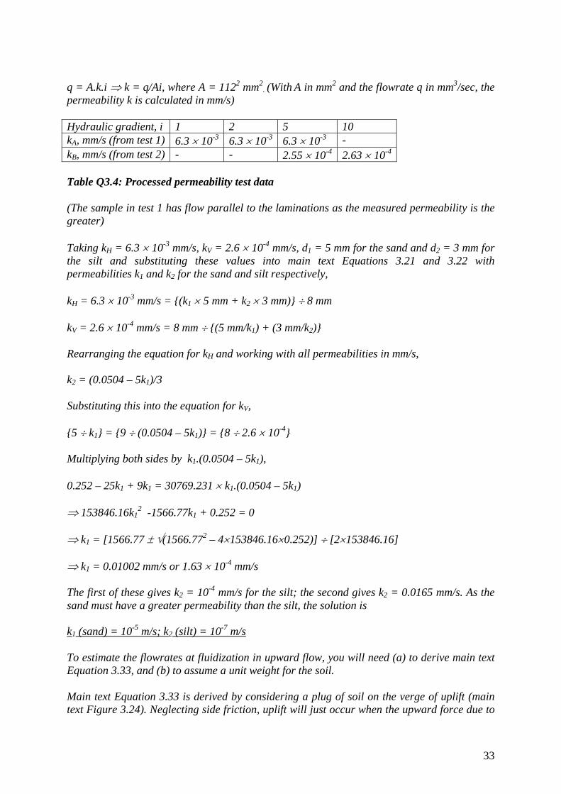
q = A.k.i ⇒ k = q/Ai, where A = 1122 mm2
. (With A in mm2 and the flowrate q in mm3/sec, the
permeability k is calculated in mm/s) Hydraulic gradient, i 1 2 5 10 kA, mm/s (from test 1) 6.3 × 10⁻³ 6.3 × 10⁻³ 6.3 × 10⁻³ - kB, mm/s (from test 2) - - 2.55 × 10⁻⁴ 2.63 × 10⁻⁴
Table Q3.4: Processed permeability test data (The sample in test 1 has flow parallel to the laminations as the measured permeability is the greater) Taking kH = 6.3 × 10⁻³ mm/s, kV = 2.6 × 10⁻⁴ mm/s, d1 = 5 mm for the sand and d2 = 3 mm for the silt and substituting these values into main text Equations 3.21 and 3.22 with permeabilities k1 and k2 for the sand and silt respectively, kH = 6.3 × 10⁻³ mm/s = {(k1 × 5 mm + k2 × 3 mm)} ÷ 8 mm kV = 2.6 × 10⁻⁴ mm/s = 8 mm ÷ {(5 mm/k1) + (3 mm/k2)} Rearranging the equation for kH and working with all permeabilities in mm/s, k2 = (0.0504 – 5k1)/3 Substituting this into the equation for kV, {5 ÷ k1} = {9 ÷ (0.0504 – 5k1)} = {8 ÷ 2.6 × 10⁻⁴} Multiplying both sides by k1.(0.0504 – 5k1), 0.252 – 25k1 + 9k1 = 30769.231 × k1.(0.0504 – 5k1) ⇒ 153846.16k1
2 -1566.77k1 + 0.252 = 0 ⇒ k1 = [1566.77 ± √(1566.772 – 4×153846.16×0.252)] ÷ [2×153846.16] ⇒ k1 = 0.01002 mm/s or 1.63 × 10⁻⁴ mm/s The first of these gives k2 = 10-4 mm/s for the silt; the second gives k2 = 0.0165 mm/s. As the sand must have a greater permeability than the silt, the solution is k1 (sand) = 10-5 m/s; k2 (silt) = 10-7 m/s
To estimate the flowrates at fluidization in upward flow, you will need (a) to derive main text Equation 3.33, and (b) to assume a unit weight for the soil. Main text Equation 3.33 is derived by considering a plug of soil on the verge of uplift (main text Figure 3.24). Neglecting side friction, uplift will just occur when the upward force due to
34
the pore water presure acting on the base (A.γw.[z+hcrit]) begins to exceed the weight of the block of soil (A.γ.z): A.γw.[z+hcrit] = A.γ.z z(γ - γw) = γw.hcrit or icrit = hcrit/z = (γ - γw)/γw (main text Equation 3.33) In the present case, we will assume γ = 2γw giving icrit = 1. At a hydraulic gradient of 1 in upward flow, the flowrates are given by the relevant permeability × the cross sectional area of the sample, 112 mm2. For test 1, qcrit = 6.3 × 10⁻³ mm/s × 112 mm2 = 79 mm3/sec (parallel to the laminations) For test 2, qcrit = 2.6 × 10⁻⁴ mm/s × 112 mm2 = 3.3 mm3/sec (perpendicular to the laminations) (These answers are slightly different from those given in the main text). Q3.5 The following data were obtained from a constant head permeameter test in downward flow on a sample of medium sand. Measured flowrate q, cm3/s 2.0 3.0 4.0 5.0 6.0 Head difference between manometer tappings ∆h, mm
18.8 31.0 45.1 60.0 75.0
Sample height z, mm 180 175 170 165 160 Specific gravity of soil grains Gs = 2.65 Cross-sectional area of permeameter A = 8 000 mm2
Distance between pressure tappings l = 120 mm Prior to the test, the sample had been brought to its loosest possible state - corresponding to a sample height of 180 mm - by fluidization in upward flow. At fluidization, the upward flowrate was 11.725 cm3/s and the head difference between the manometer tappings was 109.9 mm. Plot a graph of flowrate q against hydraulic gradient i for downward flow, and explain its shape. Estimate the maximum and minimum permeability k and specific volume v of the sample during this part of the test. [University of London 1st year BEng (Civil Engineering) examination, King's College (part question)]

35
Q3.5 Solution The hydraulic gradient is calculated as the head difference between the manometer tappings ∆h (mm) divided by the distance between them (l = 120 mm). The processed data are given in Table Q3.5 and plotted in Figure Q3.5. Flowrate q, mm3/sec 2000 3000 4000 5000 6000 Head difference ∆h, mm 18.8 31.0 45.1 60.0 75.0 Hydraulic gradient i 0.157 0.258 0.376 0.500 0.625 Table Q3.5: Processed permeameter test data
Figure Q3.5: Flowrate q against hydraulic gradient i The graph of flowrate against hydraulic gradient is curved convex upward, indicating a permeability that decreases as the flowrate is increased (the gradient of the graph is A.k and, as the cross sectional area of the sample A is a constant, the gradually reducing slope must indicate a reducing permeability). This is because as the downward flowrate is increased the sample is compacted (evidenced by the reducing sample height), decreasing both the void ratio and the permeability. The maximum permeability is with the sample in its loosest state, with the sample height z = 180 mm and the flowrate q = 2000 mm3/sec. Then k = q/Ai = 2000 mm3/sec ÷ (8000 mm2 × 0.157) ⇒ k ~ 1.6 mm/s The minimum permeability is with the sample in its densest state, with the sample height z = 160 mm and the flowrate q = 6000 mm3/sec. Then k = q/Ai = 6000 mm3/sec ÷ (8000 mm2 × 0.625) ⇒ k ~ 1.2 mm/s

36
We can calculate the unit weight of the soil at a height of 180 mm from the data given for fluidization in upward flow, using the equation derived in the main text Section 3.11 for the critical upward hydraulic gradient,
icrit = (γ – γw)/γw (main text Equation 3.33) with icrit = 109.9 mm ÷ 120 mm = 0.916 Hence at fluidization, γ = 1.916 × γw For a saturated soil, γ = γw.(Gs + v – 1)/(v) (main text Equation 1.11) where v is the specific volume, i.e. the ratio total volume Vt ÷ volume of solids Vs At fluidization, g/gw = 1.916 = (v + 1.65)/v hence 0.916v = 1.65 or vmax = 1.8 We can calculate the specific volume of the soil in the densest state, at a sample height of 160 mm, by noting that the total volume Vt is given by Vt= A.z = Vs.(Vs/Vt) = Vs.v so that v/z = A/Vs = constant = vo/zo = 1.8/180 mm = 0.01 mm-1 Hence in the densest state with z = 160 mm, v = vmin = 0.01 mm-1 × 160 mm ⇒ vmin = 1.6 Well pumping test (field measurement of permeability) Q3.6 A well pumping test was carried out to determine the bulk permeability of a confined aquifer. The aquifer was overlain by a clay layer 4 m thick, the depth of the aquifer was 20 m, and the initial piezometric level in the aquifer was 2m below ground level. After a period of pumping when steady-state conditions had been reached, the following observations were made. pumped flowrate q = 1.637 litres/second well radius = 0.1 m drawdown just outside well = 2 m drawdown in piezometer at 100m distance from well = 0.2 m Deriving from first principles any equations you need to use, determine the bulk permeability of the aquifer. Would your analysis still apply for a drawdown in the well of 4 m? [University of London 2nd year BEng (Civil Engineering) examination, Queen Mary and Westfield College]

37
Q3.6 Solution The derivation of the equation needed to solve this problem is given in full in main text Section 3.5.1. Consider the flowrate q through an annular ring around the well, concentric with the well and having a general radius r. The flow area at a general radius r is 2πrD, where D is the thickness of the aquifer. The hydraulic gradient i = -dh/dr where h is the head measured above some convenient datum. Applying Darcy's Law, q = Aki = 2πrD.k.dh/dr (main text Equation 3.12) The negative sign has been omitted from the hydraulic gradient in Equation 3.12, because we are interested in the flow towards the well, which is in the r negative direction. Rearranging Equation 3.12 and integrating between limits of (h = hw, r = rw) at the perimeter of the well and a general point (h, r) at radius r,
∫⎟⎟⎠
⎞⎜⎜⎝
⎛=∫
h
h
r
r ww
dhqkD
rdr π2
hence ln(r/rw) = (2πDk/q).(h-hw) or k = [q.ln(r/rw)] ÷ [2πD.(h-hw)] We need to think about the relationships between heads and drawdowns. Taking the datum for the measurement of head h at the bottom of the aquifer, 24 m below ground level, the initial groundwater level (at a depth of 2 m below the ground surface) corresponds to a head of 24 m – 2 m = 22 m. The drawdown just outside the well of 2 m corresponds to a head measured from the base of the aquifer of 22 m – 2 m = 20m, and the drawdown of 0.2 m at a distance of 100 m from the well corresponds to a head of 22 m – 0.2 m = 21.8 m. Substituting in the values h = 21.8 m at r = 100 m; hw = 20 m at rw = 0.1 m; D = 20 m and q = 1.637 × 10⁻³ m3/sec gives k = [1.637 × 10⁻³ m3/sec × ln (100/0.1)] ÷ [2 × π × 20 m × (21.8 m – 20 m)] ⇒ k = 5 × 10⁻⁵ m/s If the drawdown inside the well were increased to 4 m, the aquifer would become unconfined (or strong vertical flow would occur) near the well and the analysis will not strictly be valid. In reality, the error will probably be small, but will increase with increasing drawdown.

38
Confined flownets; quicksand Q3.7 Figure 3.41 shows a cross section through a square excavation at a site where the ground conditions are as indicated. Assuming that the water levels in the overlying gravels, the underlying fractured bedrock, and the medium sand outside the excavation do not change, estimate by means of a carefully-sketched flownet the capacity of the required dewatering system. What proportion of the extracted groundwater must be recirculated through the medium sand and the gravels in order to maintain the initial groundwater level in these strata, if there is no other close source of recharge? Do you foresee any problem concerning the stability of the base of the excavation? [University of London 2nd year BEng (Civil Engineering) examination, Queen Mary and Westfield College] Q3.7 Solution The flownet is sketched on Figure Q3.7, according to the rules and procedures given in the main text Sections 3.8 and 3.9.
Figure Q3.7 The flowrate q is calculated from q (m3/s per metre) = k.H.NF/NH

39
where k, the permeability of the soil = 10-4 m/s; H, the overall head drop = 10 m; NF, the number of flowtubes = 4; and NH, the number of equipotential drops, = 4 The perimeter is 8 times the half-width of the excavation, = 160 m
Hence smmmsmq /16.016044)(10)/(10 34 =×⎥⎦
⎤⎢⎣⎡ ××= −
or q = 160 litre/sec From the flownet, it may be seen that approximately 25/8 of the 4 flowtubes start in the medium sand. The proportion of the pumped groundwater that must therefore be recharged is approximately 25/8 ÷ 4 ≈ 66%. (Note that this estimate is on the high side, as some of this flow will enter the medium sand from the bedrock). The upward hydraulic gradient into the excavation is, scaling from the flownet, approximately 2.5 m ÷ 3.5 m or 0.71. While this is less than the critical value (icrit ≈ 1 for a soil with γ ≈ 2γw), it is perhaps a little close for comfort – particularly in the corners of the excavation, where flow from the two adjacent sides and the plane flownet calculation is not valid – and should therefore be investigated in more detail. Note, however, that the flownet has been drawn on the basis that there is no drawdown outside the line of the retaining wall: in reality, a drawdown in the sand outside the line of the retaining wall would move the upper equipotential further from the excavation and probably reduce the upward hydraulic gradient below the excavation floor. Q3.8 Figure 3.42 shows a plan view of an excavation underlain by a confined aquifer of uniform thickness 20m. The aquifer is bounded on two sides by a river having a water level h=12m above datum level. On the third side, the effective recharge boundary to the aquifer is as indicated. A sheet pile cut-off wall is installed along the edge of the river adjacent to the excavation, extending for a certain distance on either side. The datum level for the measurement of hydraulic head is at the upper surface of the aquifer. Estimate by means of a carefully-sketched flownet the rate at which water must be pumped from a dewatering system, in order to reduce the groundwater level at the excavation to datum level. (The permeability of the aquifer is 3.6×10⁻⁴ m/s). Explain why your analysis would be invalid for drawdowns at the excavation to below datum level. [University of London 2nd year BEng (Civil Engineering) examination, Queen Mary and Westfield College] Q3.8 Solution The flownet is sketched on Figure Q3.8. Note that this is a flownet in the horizontal plane, ie on plan, but otherwise follows exactly the same principles as a more usual flownet in the

40
cross-sectional (vertical) plan as enumerated in the main text Sections 3.8 and 3.9. In this case, the flow domain has a finite thickness, as the aquifer is confined by impermeable layers at the top and bottom.
Figure Q3.8 The flowrate q is calculated from q (m3/s per metre thickness) = k.H.NF/NH where k, the permeability of the soil = 3.6 × 10⁻⁴ m/s; H, the overall head drop = 12 m; NF, the number of flowtubes = 11; and NH, the number of equipotential drops, = 4 The thickness of the aquifer is 20 m
Hence smmmsmq /238.0204
11)(12)/(106.3 34 =×⎥⎦⎤
⎢⎣⎡ ×××= −
or q = 238 litre/sec

41
The analysis would be invalid for drawdowns below the top of the aquifer (datum level) because the flow would become unconfined. The saturated thickness of the aquifer would no longer be constant, and flow would no longer be purely horizontal and could not be represented by a two-dimensional flownet in the horizontal plane. Unconfined flownet Q3.9 Figure 3.43 shows a cross section through a long canal embankment. Explaining carefully the conditions you are attempting to fulfill, estimate by means of a flownet the rate at which water must be pumped from the drainage ditch back into the canal, in litres per hour per metre length. Describe qualitatively what might happen if the drain beneath the toe of the embankment became blocked. [University of London 2nd year BEng (Civil Engineering) examination, Queen Mary and Westfield College] Q3.9 Solution The conditions that must be fulfilled in drawing the flownet are
• equipotentials and flowlines cross at 90° • elements in the flownet have the same breadth as length, forming curvilinear squares • impermeable boundaries and the centreline are flowlines • u = 0 on the top flowline, i.e. the x m equipotential intersects the top flowline at x m
above the datum for the measurement of head (phreatic surface condition for an unconfined flownet)
The flownet is sketched on Figure Q3.9. The phreatic surface condition is satisfied by trial and error, along with the rest of the conditions above. Note: capillary rise effects are neglected.
Figure Q3.9

42
The flowrate q is calculated from q (m3/s per metre length) = k.H.NF/NH where k, the permeability of the embankment = 10-6 m/s;
H, the overall head drop = 8 m ie the level of the top surface of the canal above datum, NOT 6 m which is the level of the base of the canal and a common mistake);
NF, the number of flowtubes = 2 × 2 for symmetry = 4; and NH, the number of equipotential drops, = 4
Hence msmmsmq //10844)(8)/(10 366 −− ×=⎥⎦
⎤⎢⎣⎡ ××=
or q = 28.8 litre/hour per metre run If the drain became blocked, the top flowline would rise and emerge on the downstream face of the embankment leading to erosion and failure.. Flownets in anisotropic soils Q3.10 Figure 3.44 shows a true cross-section through a long cofferdam. It is proposed to dewater the cofferdam by lowering the water level inside it to the floor of the excavation. Investigate the suitability of this proposal by means of a carefully-sketched flownet on an appropriately-transformed cross-section (horizontal scale factor α=√kv/kh). How might the stability of the base be ensured? [University of London 2nd year BEng (Civil Engineering) examination, Queen Mary and Westfield College] Q3.10 Solution The flownet must be sketched on a transformed section, with the horizontal distances reduced by a transformation factor α = √(kv/kh) to account for the relatively higher horizontal permeability (see main text Section 3.14). α = √(kv/kh) = √(2.5 × 10⁻⁵ ÷ 10-4) = √(0.25) = 0.5 The cross section is re-drawn with the horizontal dimensions reduced by the transformation factor 0.5, and the flownet is sketched according to the rules and procedures set out in main text Sections 3.8 and 3.9, in Figure Q3.10.

43
Figure Q3.10 The flowrate q is calculated from q (m3/s per metre length) = kt.H.NF/NH where kt, the equivalent permeability of the transformed section, = √(kv.kh) (see main text Section 3.14);
kt = 5 × 10⁻⁵ m/s; H, the overall head drop = 9 m; NF, the number of flowtubes =3 × 2 for symmetry = 6; and NH, the number of equipotential drops, = 9
Hence metresmmsmq //10396)(9)/(105 345 −− ×=⎥⎦
⎤⎢⎣⎡ ×××=
or q = 0.3 litre/sec per metre length By scaling from the diagram, the vertical hydraulic gradient between the sheet piles is ~ 1, so there is a danger of base instability (quicksand or boiling). The stability of the base could be ensured by increasing the depth of the sheet piles and/or by lowering the groundwater level inside the cofferdam to well below formation level.
44
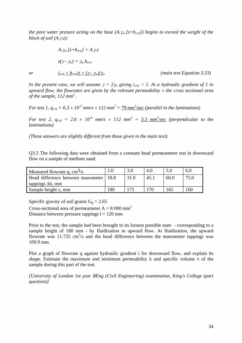
Q3.11 Figure 3.45 shows a true cross-section through a sheet-piled excavation in a laminated soil of permeability kv = 10-6 m/s (vertically) and kh = 1.6×10⁻⁵ m/s (horizontally). The laminated soil is overlain by 4 m of highly permeable gravels, and the natural groundwater level is 2 m below the soil surface. By means of a flownet sketched on a suitably-modified cross-section estimate: (a) the minimum capacity required of the dewatering system, and (b) the pore water pressure at the point A. Comment briefly on the stability of the base of the excavation. (Transformation factor α=√kv/kh) [University of London 2nd year BEng (Civil Engineering) examination, Queen Mary and Westfield College] Q3.11 Solution The flownet must be sketched on a transformed section, with the horizontal distances reduced by a transformation factor α = √(kv/kh) to account for the relatively higher horizontal permeability (see main text Section 3.14). α = √(kv/kh) = √(10-6 ÷ 1.6 ×10⁻⁵) = √(1/16) = 0.25 The cross section is re-drawn with the horizontal dimensions reduced by the transformation factor 0.25, and the flownet is sketched according to the rules and procedures set out in main text Sections 3.8 and 3.9, in Figure Q3.11.
Figure Q3.11

45
(a) The flowrate q is calculated from q (m3/s per metre length) = kt.H.NF/NH where kt, the equivalent permeability of the transformed section, = √(kv.kh) (see main text Section 3.14);
kt = 4 × 10⁻⁶ m/s; H, the overall head drop = 10 m (from the groundwater level on the retained side to the floor of the excavation);
NF, the number of flowtubes =5 (note the flownet is NOT symmetrical in this case); and NH, the number of equipotential drops, = 8
Hence metresmmsmq //105.285)(10)/(104 356 −− ×=⎥⎦
⎤⎢⎣⎡ ×××=
or q = 0.025 litre/sec per metre length (b) the point A is roughly ¼ of the way between the third and fourth equipotential lines after h = 10 m. Each equipotential drop is 10/8 = 1.25 m. Interpolating, the head at A is approximately hA ≈~ 10 m – (3.25 × 1.25 m) ≈ 5.94 m The point A is about 24.5 m below the datum for the measurement of head, giving uA = γw.(24.5 + 5.94) ≈ 300 kPa (see main text Section 3.10 and Example 3.7 for details of the calculation of pore water pressures from flownets). The upward hydraulic gradient between the sheet piles is (scaling from the flownet) approximately 1.25 m ÷ 3 m or 0.42, which is comfortably below the critical value of about 1. Thus our dewatering scheme, which involves installing pumped wells with sufficient capacity to draw down the groundwater level within the excavation to formation level, should be adequate to ensure the stability of the base.

46
QUESTIONS AND SOLUTIONS: CHAPTER 4 Analysis and interpretation of one-dimensional compression test data Q4.1 (a) What factors govern the relevance to a given design situation of the parameters obtained from an oedometer test? (b) Data from an oedometer test are given below. Show that the specific volume v is related to the sample height h by the expression (v/h) = constant. Plot a graph of specific volume v against the natural logarithm of the vertical effective stress, lnσ'v, and explain its shape. Calculate the values of κo and λo. σ'v, kPa
25 50 100 200 100 50
Equilibrium sample height h, mm (after consolidation has ceased)
19.86 19.56 19.27 18.48 18.79 19.08
Water content of sample at the end of the test (σ'v=50kPa, h=19.08mm): 20.88% Grain specific gravity Gs = 2.75 (c) Figure 4.40 shows the ground conditions at the site of a proposed new office building. The office building will have a raft foundation, the effect of which will be to increase the vertical effective stress in the clay layer by 50kPa throughout its depth. The oedometer test sample was taken from the mid-depth of the clay layer, i.e. 5m below ground level. Explaining your choice of one-dimensional modulus E'o, estimate the eventual settlement of the clay layer. What, qualitatively, would be the effect if the foundation load were to be increased by a further 50kPa? [University of London 2nd year BEng (Civil Engineering) examination, Queen Mary and Westfield College] Q4.1 Solution (a) The parameters (one dimensional stiffness, consolidation coefficient and by inference permeability) should have been obtained from tests that have reproduced as far as possible the initial stress state, the previous stress history and the expected loading or unloading increment of the soil in the field. Sample disturbance (leading to loss of fabric) might also reduce the reliability of laboratory test results; and the consolidation coefficient and permeability in the field might well be governed by preferential horizontal flow whereas in the oedometer test flow is vertical. (b) The total sample volume Vt at any stage of the test is equal to the sample area A multiplied by the current sample height h, Vt = A.h. Also, the total volume is equal to the volume of voids Vv + the volume of soil grains (solids) Vs,

47
Vt = Vs + Vv = Vs(1+Vv/Vs) = Vs.(1 + e) = Vs.v Hence
Vt = Vs.v = A.h, or vh
AV
cons ts
= = tan
Assuming that the sample is fully saturated at the end of the test, the final sample height hf can be related to the final specific volume vf by measurement of the final moisture content wf, vf = (1 + ef ) = (1 + wf . Gs) = 1 + (0.2088 × 2.75) = 1.5742
hence 11 0825.008.19
5742.1 −− ===== mmmmh
vonstantc
VA
hv
f
f
s
Convert the values of h to values of v using v = 0.0825 × h, σ’v, kPa 25 50 100 200 100 50 h, mm 19.86 19.56 19.27 18.48 18.79 19.08 ln σ’v 3.219 3.912 4.605 5.298 4.605 3.912 v 1.639 1.614 1.590 1.525 1.550 1.574 Plot v against lnσ’v (Figure Q4.1)
Figure Q4.1: v against ln(σ'v)

48
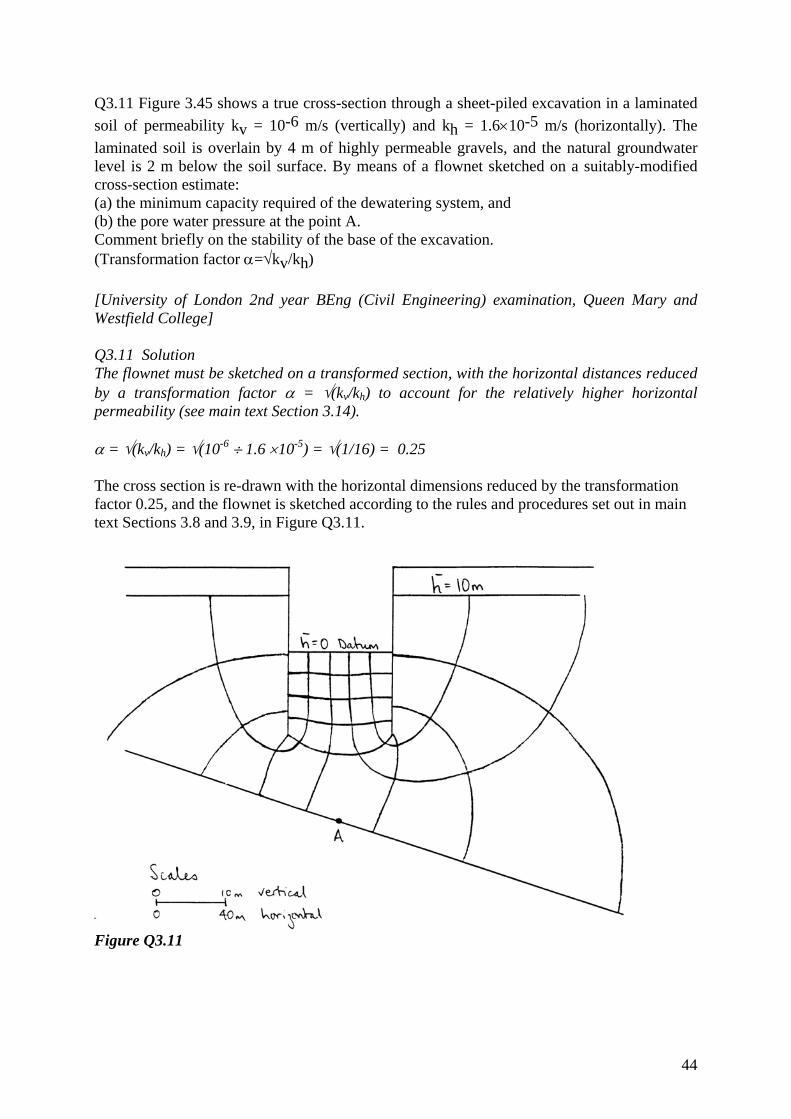
A – B: reloading, “elastic” (recoverable) deformation only B: maximum previous preconsolidation pressure, sample moves onto normal (first)
compression line B – C: normal (first) compression: “elastic” plus plastic (irrecoverable) deformation. Plastic
deformation is due to particle slip C – D: unloading; “elastic” component of deformation is recovered The soil is overconsolidated along AB and CD, and normally consolidated along BC. The slope of the reloading and unloading lines is –κ0; the slope of the one-dimensional normal compression line is -λ0 From the graph or the data,
035.050ln100ln
639.1590.1'ln
=−−
−=∆
∆−=
vo
vσ
κ
(the slope of the unloading line), and
094.0100ln200ln
590.1525.1'ln
=−−
−=∆
∆−=
vo
vσ
λ
(the slope of the one dimensional normal compression line). (c) The initial vertical effective stress at the centre of the clay layer is approximately (20 kN/m3 × 5 m) – (10 kN/m3 × 5 m) = 50 kPa. The vertical effective stress is then increased (after the dissipation of excess pore water pressures) to 100 kPa. The appropriate stress range is therefore 50 to 100 kPa. Over this stress increment, the sample height reduced by (19.56 – 19.27) = 0.29 mm. Assuming that the same value of one-dimensional modulus applies, the eventual settlement of a 5 m thick layer of the same clay is 0.29 mm × (5000 mm ÷ 19.56 mm) = 74 mm. (Note there is no need to calculate the value of E'0 explicitly). If the vertical effective stress at the centre of the clay layer were increased to more than 100 kPa, the soil state would move from a (comparatively stiff) reload line to the much less stiff normal compression line, as the precompression stress was exceeded. This would lead to comparatively larger settlements (e.g. in going from 100 kPa to 200 kPa, the oedometer test sample compresses by 0.79 mm giving an equivalent settlement of the 5 m layer of 0.79×5000/19.27 = 205 mm. Assuming a logarithmic increase in stiffness with stress, 70% of this settlement i.e. 142 mm would occur on increasing the vertical effective stress from 100 to 150 kPa).

49
Q4.2 (a) Describe with the aid of a diagram the important features of a conventional oedometer, and define the parameters that this apparatus is used to measure. (b) Data from an oedometer test on a sample of clay are given below. σ'v, kPa
50 100 200 400 800 600 400
Equilibrium sample height h, mm
17.123 16.912 16.701 15.496 14.300 14.390 14.521
Cross-sectional area of sample = 80 000 mm2 Gs = 2.61 Two-way sample drainage Water content at start of test: 45.14% Water content at end of test: 32.84% Calculate the specific volume at the end of the test, assuming Sr=1 at this stage. What was the saturation ratio at the start of the test? Show that the specific volume is related to the sample height by the expression v/h = A/vs = constant, where A is the cross sectional area of the sample and vs is the volume occupied by the soil grains. Plot a graph of the specific volume against the natural logarithm of the vertical effective stress. Explain the shape of this graph. Calculate the preconsolidation pressure and the slopes of the one-dimensional normal compression line and unloading/reloading lines. [University of London 2nd year BEng (Civil Engineering) examination, King's College (part question)] Q4.2 Solution (a) A diagram of the oedometer is given in the main text Figure 4.2. The apparatus is used to measure
i) the stiffness of the soil in one dimensional compression, E'0, over a given stress range;
ii) the coefficient of consolidation, cv = kv.E'0/γw iii) by inference, the vertical permeability kv.
(b) Assuming that the sample is fully saturated at the end of the test, the specific volume at this stage is given by vf = (1 + ef ) = (1 + wf . Gs) = 1 + (0.3284× 2.61) = 1.857 At the start of the test, the specific volume is equal to 1.857 × (17.123 ÷ 14.521) = 2.190. The saturation ratio may be calculated using

50
Sr = w.Gs/(v – 1) (main text Equation 1.10) or Sr = 0.4514 × 2.61 ÷ 1.190 = 99% The total sample volume Vt at any stage of the test is equal to the sample area A multiplied by the current sample height h, Vt = A.h. Also, the total volume is equal to the volume of voids Vv + the volume of soil grains (solids) Vs, Vt = Vs + Vv = Vs(1+Vv/Vs) = Vs.(1 + e) = Vs.v Hence
Vt = Vs.v = A.h, or vh
AV
cons ts
= = tan
The numerical value of the constant is equal to the specific volume divided by the sample height at the end of the test,
11 1279.0521.14
857.1 −− == mmmmh
v
f
f
Convert the values of h to values of v using v = 0.1279 × h, σ’v, kPa 50 100 200 400 800 600 400 h, mm 17.123 16.912 16.702 15.496 14.300 14.390 14.521 ln σ’v 3.912 4.605 5.298 5.991 6.685 6.397 5.991 v 2.190 2.163 2.136 1.982 1.829 1.840 1.857 Plot v against lnσ’v (Figure Q4.2)
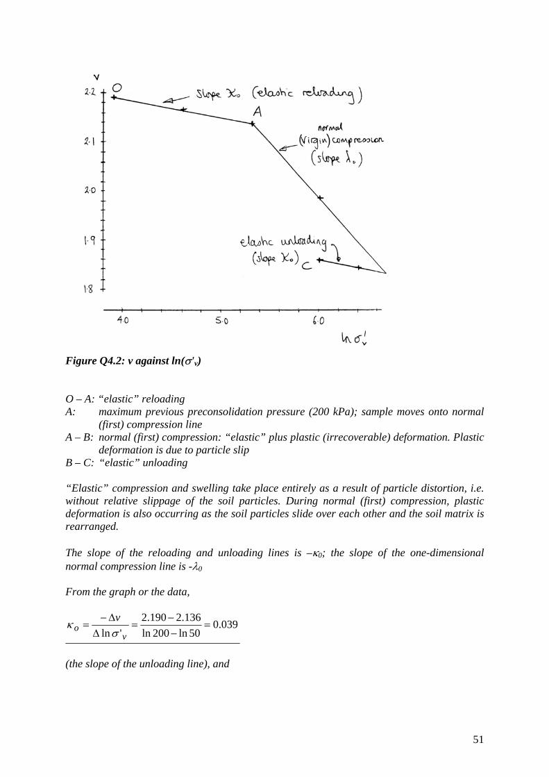
51
Figure Q4.2: v against ln(σ'v) O – A: “elastic” reloading A: maximum previous preconsolidation pressure (200 kPa); sample moves onto normal
(first) compression line A – B: normal (first) compression: “elastic” plus plastic (irrecoverable) deformation. Plastic
deformation is due to particle slip B – C: “elastic” unloading “Elastic” compression and swelling take place entirely as a result of particle distortion, i.e. without relative slippage of the soil particles. During normal (first) compression, plastic deformation is also occurring as the soil particles slide over each other and the soil matrix is rearranged. The slope of the reloading and unloading lines is –κ0; the slope of the one-dimensional normal compression line is -λ0 From the graph or the data,
039.050ln200ln
136.2190.2'ln
=−
−=
∆∆−
=v
ov
σκ
(the slope of the unloading line), and

52
221.0200ln800ln829.1136.2
'ln=
−−
=∆
∆−=
vo
vσ
λ
(the slope of the one dimensional normal compression line). The preconsolidation pressure (i.e. the maximum previous value of vertical effective stress, at which the soil moves from a reload line onto the one dimensional normal compression line, is σ'v, maximum previous = 200 kPa (see above) Q4.3 For the oedometer test described in Q4.2, plot a graph of vertical effective stress σ'v against vertical strain εv. For each of the loading and unloading steps, calculate the one-dimensional modulus E'o = ∆σ'v/∆εv (∆σ'v and ∆εv are the changes in vertical effective stress and strain that occur during the loading or unloading step.) Comment briefly on the significance of these results in the context of the selection of parameters for design. Q4.3 Solution For each load increment or decrement, the one-dimensional modulus E'o is defined as the change in vertical effective stress ∆σ'v divided by the change in vertical strain ∆εv. The change in vertical strain during a load increment or decrement is based on the equilibrium sample height at the start of that increment or decrement.
Load increment/ decrement, kPa
50-100 100-200 200-400 400-800 800-600 600-400
∆σ'v, kPa 50 100 200 400 -200 -200 change in sample height ∆h, mm
0.211 0.211 1.205 1.196 -0.090 -0.131
vertical strain during increment ∆εv = ∆h/ho
0.0123
0.0125 0.0722 0.0772 -0.0063 -0.0091
E'o = ∆σ'v/∆εv, MPa
4.06 8.02 2.77 5.18 31.78 21.97
Notes: (1) The initial sample height ho is taken as the sample height at the start of the each load increment or decrement. (2) Negative stress and strain increments are tensile, correponding to unloading and sample heave. (3) When calculating E'o in MPa, remember to allow for the fact that ∆σ'v is in kPa.

53
Even for small changes in stress, the soil stiffness is clearly dependent on the initial stress state, whether the sample is being loaded or unloaded and whether the soil is normally or over consolidated. In determining an appropriate stiffness for use in a design calculation, it is necessary to replicate the stress history, stress state and anticipated stress path of the soil in the field. Analysis of data from the consolidation phase Q4.4 Data from one stage of an oedometer test are given below. Time, min 0.25 1 4 9 16 25 Settlement mm
0.063 0.075 0.103 0.133 0.160 0.185
Time, min 36 49 64 81 100 196 Settlement mm
0.210 0.228 0.240 0.250 0.258 0.265
Load increment: 25 - 50 kPa Sample diameter: 76 mm Initial sample thickness: 20 mm Two-way drainage For this load increment, estimate the one-dimensional modulus E'o, the consolidation coefficient cv, and the vertical permeability of the soil kv. (It may be assumed that the initial slope of a graph of proportional settlement R=ρ/ρult against the square root of the time factor
T=cvt/d2 is equal to √(4/3), ie R = √(4T/3).) What factors would you take into account in the laboratory determination of E'o cv and kv for use in design? What difficulties might you encounter in attempting to use oedometer test results to predict rates of settlement in the field? [University of London 2nd year BEng (Civil Engineering) examination, Queen Mary and Westfield College (part question)] Q4.4 Solution Plot a graph of settlement against√ time (Figure Q4.4): time t, min 0.25 1 4 9 16 25 36 49 64 81 100 196 settlement ρ, mm
.063 .075 .103 .133 .160 .185 .210 .228 .240 .250 .258 .265
√t, min0.5 0.5 1 2 3 4 5 6 7 8 9 10 14
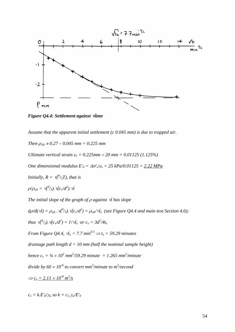
54
Figure Q4.4: Settlement against √time Assume that the apparent initial settlement (c 0.045 mm) is due to trapped air. Then ρult ≈ 0.27 – 0.045 mm = 0.225 mm Ultimate vertical strain εv = 0.225mm ÷ 20 mm = 0.01125 (1.125%) One dimensional modulus E'0 = ∆σ'v/εv = 25 kPa/0.01125 = 2.22 MPa Initially, R = √(4/3T), that is ρ/ρult = √(4/3).√(cv/d2).√t The initial slope of the graph of ρ against √t has slope dρ/d(√t) = ρult .√(4/3).√(cv/d2) = ρult/√tx (see Figure Q4.4 and main text Section 4.6); thus √(4/3).√(cv/d2) = 1/√tx or cv = 3d2/4tx From Figure Q4.4, √tx = 7.7 min0.5 ⇒ tx = 59.29 minutes drainage path length d = 10 mm (half the nominal sample height) hence cv = ¾ × 102 mm2/59.29 minute = 1.265 mm2/minute divide by 60 × 10-6 to convert mm2/minute to m2/second ⇒ cv = 2.11 × 10⁻⁸ m2/s cv = k.E'0/γw so k = cv.γw/E'0
55
k = 2.11 × 10⁻⁸ m2/s × 9.81 kN/m3 ÷ 2222 kN/m2 ⇒ k = 9.3 × 10⁻¹¹ m/s (Note: the answer for permeability given at the end of Q4.4 in the main text is not correct) In determining parameter values for design, the following factors should be taken into account and replicated as far as possible in the laboratory test.
• the stress state of the soil in the field • the stress history of the deposit • the changes in stress to which the soil will be subjected
Difficulties in applying laboratory-determined parameters to field problems include
• uncertainty concerning field drainage path lengths and boundary conditions • E'0 is the stiffness in one-dimensional compression – the true strain path in the field is
unlikely to be one dimensional and will vary from point to point • soil parameters are not constant, but vary with stress state and strain • large scale fabric effects can be difficult to take into account • drainage in the field is likely to be horizontal, whereas the oedometer test gives the
vertical permeability of the soil. Q4.5 An engineer carries out an oedometer consolidation test on a sample of stiff clay, in connexion with the design of a proposed grain silo. The results from this test are as follows: Time, min 0 0.5 1 2 4 8 16 32 64 Settlement mm
0.020 0.044 0.052 0.066 0.086 0.110 0.150 0.192 0.216
Load increment: 100 - 200 kPa Initial sample thickness: 20 mm Two-way drainage Suggest a reason for the initial settlement of 0.02 mm. Estimate the one dimensional modulus E'o and the consolidation coefficient cv for the clay over the stress range under consideration. (It may be assumed that a graph of the consolidation settlement ρ against the square root of the elapsed time t has an initial slope of ρult.√(4cv/3d2), ie that ρ = ρult.√(4cvt/3d2).) [University of London 2nd year BEng (Civil Engineering) examination, King's College (part question)] Q4.5 Solution Plot a graph of settlement against√ time (Figure Q4.5): time t, min 0 0.5 1 2 4 8 16 32 64 settlement ρ, mm .020 .044 .052 .066 .086 .110 .150 .192 .216
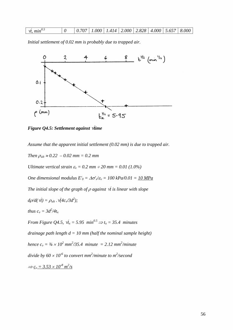
56
√t, min0.5 0 0.707 1.000 1.414 2.000 2.828 4.000 5.657 8.000 Initial settlement of 0.02 mm is probably due to trapped air.
Figure Q4.5: Settlement against √time Assume that the apparent initial settlement (0.02 mm) is due to trapped air. Then ρult ≈ 0.22 – 0.02 mm = 0.2 mm Ultimate vertical strain εv = 0.2 mm ÷ 20 mm = 0.01 (1.0%) One dimensional modulus E'0 = ∆σ'v/εv = 100 kPa/0.01 = 10 MPa The initial slope of the graph of ρ against √t is linear with slope dρ/d(√t) = ρult .√(4cv/3d2); thus cv = 3d2/4tx From Figure Q4.5, √tx = 5.95 min0.5 ⇒ tx = 35.4 minutes drainage path length d = 10 mm (half the nominal sample height) hence cv = ¾ × 102 mm2/35.4 minute = 2.12 mm2/minute divide by 60 × 10-6 to convert mm2/minute to m2/second ⇒ cv = 3.53 × 10⁻⁸ m2/s

57
Application of one-dimensional compression and consolidation theory to field problems Q4.6 Figure 4.41 shows a cross section through a long sheet piled excavation. The width of the excavation is b, its depth is h and the sheet piles penetrate a further depth d to a permeable aquifer. A standpipe piezometer is driven into the aquifer, and the water in the standpipe rises to a height H above the bottom of the sheet piles. (a) Show that the base of the excavation will become unstable if H > Hcrit, where (Hcrit)>d.γ/γw. (Note: this is a quicksand problem: see Section 3.11.) (b) Some time after the excavation has been made, and steady state seepage from the aquifer to the excavation floor has been established, it is found that H is indeed very close to Hcrit. In order to reduce the risk of base instability it is decided to reduce the head in the aquifer to H/2 by pumping. This is done very rapidly. Explain why the pore water pressures in the soil between the sheet piles cannot respond instantaneously. (c) Taking d=10 m, γ = 20 kN/m3 and γw = 10 kN/m3, draw diagrams to show the initial and final distributions of pore water pressure with depth in the soil between the sheet piles. Draw also the initial and final distributions of excess pore water pressure with depth, and sketch in three or four isochrones at various stages in between. (d) The soil between the sheet piles has a one dimensional modulus E'o that increases linearly with depth from 5 MPa at the excavated surface to 45 MPa at the interface with the aquifer. Estimate the settlement which ultimately results from the reduction in pore water pressure due to pumping. [University of London 2nd year BEng (Civil Engineering) examination, King's College] Q4.6 Solution (a) Upward flow between the sheet piles is one dimensional. Given that the bounding equipotentials (the top of the underlying aquifer, where the head is H above the bottom of the sheet piles; and the excavation surface, where the head is d above the bottom of the sheet piles) are parallel to each other and perpendicular to the bounding flowlines (the sheetpiles), the hydraulic gradient between the sheet piles is uniform and given by i = ∆h/∆z = (H – d)/d = (H/d) – 1 Instability will occur when the actual value of i reaches the critical value icrit, given by icrit = (γ – γw)/γw = (γ/γw) – 1 (see main text Section 3.11 for the derivation of this expression) Hence instability will occur when H = Hcrit = d.γ/γw (b) The pore water pressures in the soil between the sheet piles cannot respond instantaneously because this would require a change in effective stress (the total stress remains constant). A change in effective stress requires a change in volume, which requires

58
water to drain out of or into the soil, which can only occur at a rate governed by the soil permeability. (c) Initially the pore water pressure varies linearly with depth from zero at the excavated surface (z = 0) to γw.Hcrit = γ.d = 200 kPa at the bottom of the sheet piles (z = 10 m). Finally, the variation in pore water pressure is linear between zero at the excavated surface and 100 kPa at depth z = 10 m (hydrostatic). The initial and final distributions of pore water pressure with depth are shown in Figure Q4.6a; subtracting the hydrostatic or steady state component, the corresponding distributions of excess pore water pressure, together with some isochrones in between, are shown in Figure Q4.6b (compare with main text Figure 4.25, and note that the excess pore water pressure in the aquifer at the lower drainage boundary can drop to zero immediately).
(a) (b)
Figure Q4.6: distributions of (a) pore water pressure and (b) excess pore water pressure (with hydrostatic or steady state component subtracted) with depth (d) Consider an element of soil of thickness δz at a depth z below the excavated surface. The compression of this element is δρ, given by δρ = (∆σ'v/E'0).δz as by definition E'0 = ∆σ'v/∆εv and ∆εv = δρ/δz Now, E'0 = (5000 + 4000z) kPa and the eventual increase in vertical effective stress ∆σ'v at depth z is equal to the reduction in pore water pressure at the same depth, ∆σ'v = 10z (ignoring friction on the sheet piles). Hence the total settlement ρ is given by

59
∫+
==
=
mz
zdz
zz10
0 4000500010ρ
Let u = 5000 + 4000z then z = (u – 5000)/4000 and dz = du/4000, and
( )4000
.400/500045000
5000
duu
u∫
−=ρ
= duu∫ ⎟
⎠⎞
⎜⎝⎛ −
45000
5000 1600050
16000001 = ⎥⎦
⎤⎢⎣⎡ −
16000)ln(.50
1600000
45000
5000
uu (settlement in metres)
Thus ρ = (0.028 – 0.033) – (0.003 – 0.027) m = 0.019 m or ρ = 19 mm Q4.7 Figure 4.42 shows the ground conditions at the site of the Jubilee Line Extension station at Canary Wharf, in East London. During construction of the station, it was necessary to lower the groundwater level at the top of the Thanet Sands to 84m above site datum. (a) Assuming that the groundwater level in the Thames Gravels is unaffected, and that the groundwater level at the top of the Chalk is reduced by only 35kPa, construct a table for the soil behind the retaining wall, showing the initial and final vertical effective stresses at the ground surface and at the interface levels between each of the strata. (b) Using the geotechnical data given in Figure 4.42, estimate i. the immediate settlement of the soil surface, ii. the long term settlement of the soil surface, and iii. using the relation between R and T given in Figure 4.18, the settlement after a period of 18 months. Take the unit weight of water γw=10 kN/m3. [University of London 2nd year BEng (Civil Engineering) examination, Queen Mary and Westfield College]
60
Q4.7 Solution Calculate the initial and final stresses at the top and bottom of each layer: Level, m above SD
σv, kPa
u initial, kPa
σ'v initial, kPa
u final, kPa
σ'v final, kPa
∆σ'v, kPa
105 0 0 0 0 0 0 98 126 0 126 0 126 0 94 210 40 170 40 170 0 84 420 95 325 0 420 +95 70 714 235 479 200 514 +35 i) Initial settlement is due to compression of the Thanet Sands, which will occur very quickly owing to their relatively high permeability and stiffness. E'0 = ∆σ'v/εv εv = ρ/x Therefore settlement ρ = ∆σ'v.x/E'0 For the Thanet Sands, ∆σ'v (average) = (95 kPa + 35 kPa)/2 = 65 kPa ρ = 65 kPa × 14 m ÷ 200 MPa = 4.6 mm ii) Ultimate settlement is due to compression of the Thanet Sands plus consolidation of the Woolwich & Reading Beds (now known as the Lambeth Group). For the Woolwich & Reading Beds, ∆σ'v (average) = (95 kPa)/2 = 47.5 kPa ρ = 47.5 kPa × 10 m ÷ 40 MPa = 11.875 mm Total ultimate settlement = 4.6 mm + 11.9 mm = 16.5 mm (iii) Calculate the time factor T = cv.t/d2 after t = 18 months: The Woolwich & Reading Beds have two-way drainage, so drainage path length d = 10 m ÷ 2 = 5 m. Hence T = 4 m2/year × 1.5 year ÷ 52 m2 = 0.24 Φροµ µαιν τεξτ Φιγυρε 4.18, τηισ χορρεσπονδσ το α προπορτιοναλ σεττλεµεντ Ρ = ρ/ρult = 0.58 Hence the settlement after 18 months = 4.55 mm (Thanet Sands) + (0.58 × 11.875 mm) (Woolwich & Reading Beds) = 11.4 mm

61
QUESTIONS AND SOLUTIONS: CHAPTER 5 Interpretation of triaxial test results Q5.1 Data from a conventional, consolidated-undrained triaxial compression test, carried out at a constant cell pressure of 400 kPa, are given below. Axial strain εa, % 0 0.05 0.09 0.18 0.39 0.69 1.51 Deviator stress q, kPa 0 10.9 22.3 33.5 45.0 53.5 65.4 Pore water pressure u, kPa 274.6 280.3 284.6 290.8 300.0 307.6 314.4 Axial strain εa, % 3.22 4.74 6.13 7.89 9.39 11.03 Deviator stress q, kPa 79.0 85.7 89.6 91.4 93.9 94.0 Pore water pressure u, kPa 317.0 315.1 312.6 312.1 312.7 312.8 Plot graphs of mobilized strength φ'mob and pore water change ∆u against shear strain γ. Plot also the total and effective stress paths in the q,p and q,p' planes. Comment on these curves, and estimate the critical state strength φ'crit. Is the sample lightly or heavily overconsolidated? Q5.1 Solution Convert the data to the required format using the following equations (for derivations and justifications, see the main text Section 5.4 etc): γ=1.5εa (main text Figure 5.7) t = (σ'1-σ'3)/2 (main text Equation 5.1) s' = (σ'1+σ'3)/2 (main text Equation 5.2) φ'mob = sin-1(t/s') (main text Figure 5.6) q = σ'a-σ'r = σa-σr = σa-σc (main text Equation 5.6) p'=σc-u+q/3 (main text Equation 5.10) p=σc+q/3. (main text Equation 5.11) Now, t = (σ'1-σ'3)/2 = (σ1-σ3)/2 = (σa-σc)/2 = q/2 and s' = (σ'1+σ'3)/2 = [(σ1+σ3)/2]-u = [(σa+σc)/2]-u
62
hence s' = σc + q/2 - u and φ'mob = sin-1{q/(2σc + q - 2u) Also, the change in pore water pressure ∆u = u - uo, where uo is the pore water pressure at the start of shear (= 274.6kPa in this case). Hence Axial strain εa, % 0 0.05 0.09 0.18 0.39 0.69 1.51 Shear strain γ = 1.5×εa, % 0 0.075 0.135 0.27 0.585 1.035 2.265 Deviator stress q, kPa 0 10.9 22.3 33.5 45.0 53.5 65.4 Pore water pressure u, kPa 274.6 280.3 284.6 290.8 300.0 307.6 314.4 ∆u = u - uo, kPa 0 5.7 10.0 16.2 25.4 33.0 39.8 φ'mob =
sin-1{q/(2σc + q - 2u), °
0 2.4 5.1 7.6 10.6 13.0 16.0
p = σc + q/3, kPa 400 403.6 407.4 411.2 415.0 417.8 421.8 p' = σc + q/3 - u, kPa 125.4 123.3 122.8 120.4 115.0 110.2 107.4 Axial strain εa, % 3.22 4.74 6.13 7.89 9.39 11.03 Shear strain γ = 1.5×εa, % 4.83 7.11 9.20 11.84 14.1 16.5 Deviator stress q, kPa 79.0 85.7 89.6 91.4 93.9 94.0 Pore water pressure u, kPa 317.0 315.1 312.6 312.1 312.7 312.8 ∆u = u - uo, kPa 42.4 40.5 38.0 37.5 38.1 38.2 φ'mob =
sin-1{q/(2σc + q - 2u), °
18.8 19.6 19.8 20.0 20.5 20.5
p = σc + q/3, kPa 426.3 428.6 429.9 430.5 431.3 431.3 p' = σc + q/3 - u, kPa 109.3 113.5 117.3 118.4 118.6 118.5 (Calculated values are shown in bold type) Graphs of mobilized strength φ'mob and pore water change ∆u against shear strain γ, and the total and effective stress paths in the q,p and q,p' planes, are plotted in Figures Q5.1a and b. There is no peak strength, and the sample has positive pore water pressures at failure. The sample is therefore probably wet of critical, i.e. lightly overconsolidated. The effective stress path appears to follow an undrained state boundary, but near the end veers off to the right (i.e. the pore water pressures start to reduce) to reach the critical state line at a higher value of q (and p') than might otherwise have been expected. The reason for this is unclear, but possible causes include the development of a rupture and/or sample anisotropy.

63
From Figure Q5.1a, φ'crit ≈ 20½°.
Figure Q5.1a: mobilized strength φ'mob and change in pore water pressure ∆υ against shear strain γ
Figure Q5.1b: total and effective stress paths, q against p and q against p'
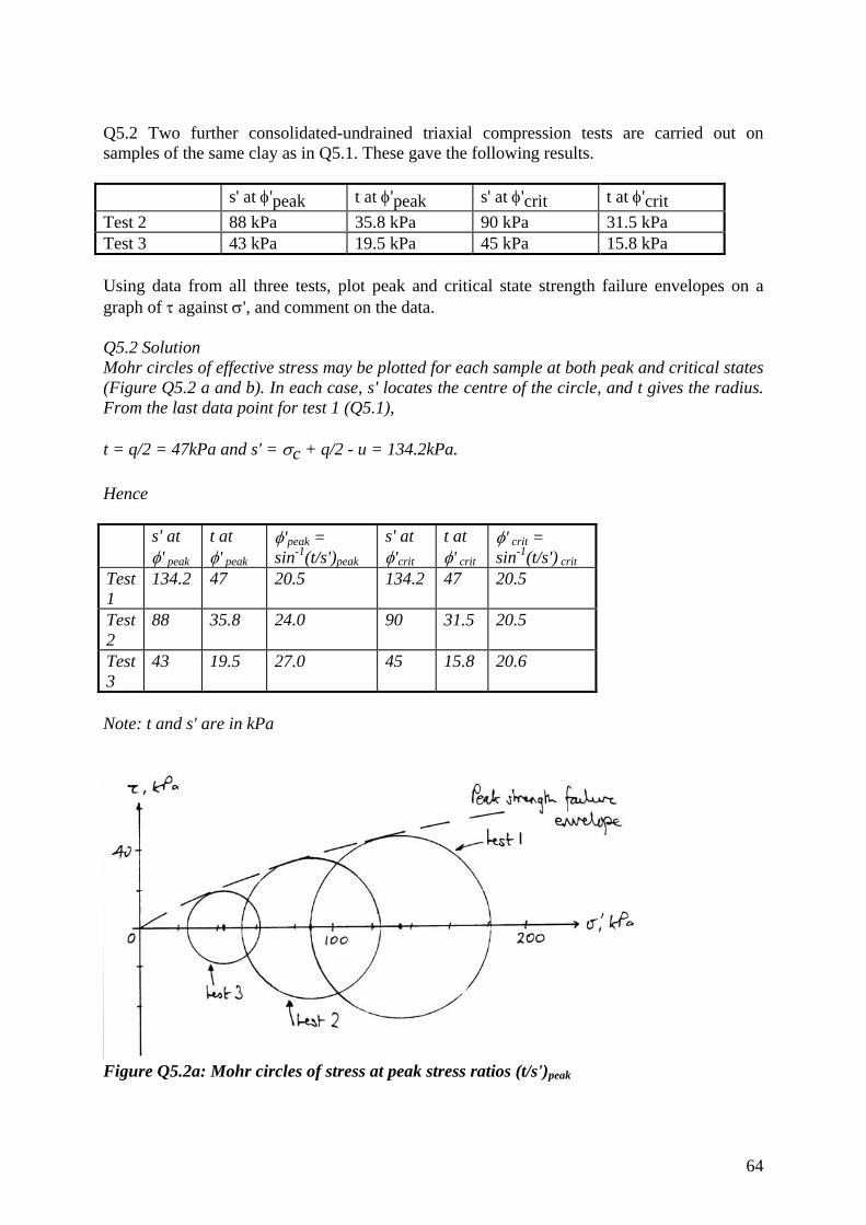
64
Q5.2 Two further consolidated-undrained triaxial compression tests are carried out on samples of the same clay as in Q5.1. These gave the following results. s' at φ'peak t at φ'peak s' at φ'crit t at φ'crit Test 2 88 kPa 35.8 kPa 90 kPa 31.5 kPa Test 3 43 kPa 19.5 kPa 45 kPa 15.8 kPa Using data from all three tests, plot peak and critical state strength failure envelopes on a graph of τ against σ', and comment on the data. Q5.2 Solution Mohr circles of effective stress may be plotted for each sample at both peak and critical states (Figure Q5.2 a and b). In each case, s' locates the centre of the circle, and t gives the radius. From the last data point for test 1 (Q5.1), t = q/2 = 47kPa and s' = σc + q/2 - u = 134.2kPa. Hence s' at
φ' peak t at φ' peak
φ'peak = sin-1(t/s')peak
s' at φ'crit
t at φ' crit
φ' crit = sin-1(t/s') crit
Test 1
134.2 47 20.5 134.2 47 20.5
Test 2
88 35.8 24.0 90 31.5 20.5
Test 3
43 19.5 27.0 45 15.8 20.6
Note: t and s' are in kPa
Figure Q5.2a: Mohr circles of stress at peak stress ratios (t/s')peak

65
Figure Q5.2b: Mohr circles of stress at critical stress ratios (t/s')crit The peak strength failure envelope is curved due to the decreasing effect of the dilational component of strength as the effective stress is increased, with φ'peak (defined as tan-
1[τ/σ']peak = sin-1[t/s']peak) decreasing from 27° in test 3 to 20½° in test 1. The critical state failure envelope is a straight line through the origin with φ'crit ≈ 20½°. Q5.3 Using the data from Q5.1 and Q5.2, determine the equations of the critical state line in the q,p' and v,lnp' planes. (The as-tested water contents were 41.7% for sample 1; 45.5% for sample 2; and 52.0% for sample 3. Take Gs = 2.65). Hence predict the undrained shear strength of a fourth sample of the same clay, which is subjected to a conventional undrained triaxial compression test at a water content of 35%. Q5.3 Solution We can calculate the values of q and p' at the critical state for tests 2 and 3 from the values of t and s' given: t = q/2, s' = (σc - u) + q/2 ⇒ (σc- u) = s' - q/2 and p' = (σc-u) + q/3 = s' - q/6 We can calculate the specific volume v for each test using v = 1 + e with

66
e = w.Gs Hence, at the critical state, s', kPa t, kPa p', kPa q, kPa v lnp' Test 1 - - 118.5 94.0 2.105 4.775 Test 2 90 31.5 79.5 63.0 2.206 4.376 Test 3 45 15.8 39.7 31.6 2.378 3.681 Graphs of q against p' and v against lnp' at critical states are shown in Figures Q5.3 a and b.
Figure Q5.3a: q against p' at critical states

67
Figure Q5.3b: v against lnp' at critical states From these graphs, the critical state line equations are q = 0.793×p', i.e.Μ = 0.793 and v = 3.3 - 0.25×lnp', i.e. Γ = 3.3 andλ = 0.25 The fourth sample has w = 35% ⇒v = 1.9275, giving p'cs = e{(Γ-v)/λ} =e{(3.3-1.9275)/0.25} = 242.26kPa Then the undrained shear strength τu = qcs/2 = M.p'cs/2 = 96.1 kPa

68
Determination of critical state and Cam clay parameters Q5.4 Define in terms of principal stresses and the quantities measured during a conventional undrained compression test the parameters q, p and p'. Data from both consolidation and shear stages of an undrained triaxial compression test on a sample of reconstituted London clay are given below. Plot the state paths followed by the sample on graphs of q against p', q against p and v against lnp', and explain their shapes. CP,kPa 50 100 200 150 150 150 150 150 q, kPa 0 0 0 0 21 39 61 86 u, kPa 0 0 0 0 7 13 43 82 v 2.228 2.116 2.005 2.023 2.023 2.023 2.023 2.023 CP: cell pressure q: deviator stress u: pore water pressure v: specific volume Stating clearly the assumptions you need to make, estimate the soil parameters Μ, λ, κ and φ'crit. [University of London 2nd year BEng (Civil Engineering) examination, Queen Mary and Westfield College] Q5.4 Solution q = deviator stress = σ1 – σ3 = σ'1 - σ'3 q = the ram load Q divided by the current sample area A. In an undrained test the total volume Vt is constant = A0.h0 = A.h = A.h0.(1 – εax) where εax is the axial strain ∆h/h0, hence A = A0/(1 – εax) and q = Q.(1 – εax)/A0 p = average total stress = 1/3(σ1 + σ2 + σ3) p' = average effective stress = p – u u = pore water pressure (measured); σ2 = σ3 = cell pressure CP (measured); σ1 = cell pressure CP + q, so p = CP + q/3 The processed data (to obtain p' and lnp') are tabulated below

69
CP,kPa 50 100 200 150 150 150 150 150 q, kPa 0 0 0 0 21 39 61 86 u, kPa 0 0 0 0 7 13 43 82 v 2.228 2.116 2.005 2.023 2.023 2.023 2.023 2.023 p, kPa 50 100 200 150 157 163 170.3 178.7 p', kPa 50 100 200 150 150 150 127.3 96.7 lnp'(p' in kPa)
3.912 4.605 5.298 5.011 5.011 5.011 4.847 4.572
Point on graphs
A B C Y F
The state paths followed on graphs of q against p and p', and v against ln p', are plotted in Figure Q5.4.
(a) (b)
Figure Q5.4: (a) q against p and p'; (b) v against ln p' A to B is isotropic normal compression, with increasing cell pressure, drainage taps open and no deviator (shear) stress applied. It is first loading, so changes in specific volume are mainly plastic (irrecoverable) B to C is isotropic unloading (reduction in cell pressure with the drainage taps open and no shear). The elastic component of volumetric compression that occurred during loading over the same stress range is recovered.
70
C to Y is undrained shear (cell pressure constant, drainage taps cloase, deviator stress applied) within the initial yield locus set up by isotropic compression to C. Behavious is “elastic” within the initial yield locus, so as there is no change in specific volume there can be no change in average effective stress and p' = constant. At Y, the sample reaches the initial yield locus and yields. This is the transition point to plastic behaviour. From Y to F, the sample is sheared at constant specific volume. To move the state of the sample to the appropriate point on the critical state line, the average effective stress must decrease and the pore water pressure increases to achieve this. At F, the sample reaches the critical state appropriate to the specific volume as tested, at which continued deformation can take place at constant q, p' and v. Assuming that A to B is on the isotropic normal compression line and that F is on the critical state line, the critical state paramaters Μ, λ and κ may be calculated as follows. Μ = q/p' at the critical state F ⇒ Μ = 86/96.7 = 0.89 λ the slope of the isotropic normal compression line = -∆v/∆ln p' between A and B: λ = (2.228 – 2.005)/(5.298 – 3.912) ⇒ λ = 0.161 κ the slope of an unload/reload line = -∆v/∆ln p' between B and C: κ = (2.023 – 2.005)/(5.298 – 5.011) ⇒ κ = 0.063 From main text Equation 5.32a, sinφ'crit = (3Μ)/(6 + Μ) = (3 × 0.89)/(6 + 0.89) ⇒ φ'crit = 22.8° Q5.5 Define the parameters q, p and p', in terms of principal stresses. Show also how q, p and p' are related to the quantities measured during a conventional undrained compression test. Data from the shear stage of an undrained triaxial compression test on a sample of kaolin clay are given below. Plot the state paths followed by the sample in the q:p' and q:p planes, and explain their shapes. Stating clearly the assumptions you need to make, estimate the slope of the critical state line Μ and the corresponding value of φ'crit. q, kPa 0 13.8 27.5 41.3 53.0 59.5 63.0 u, kPa 0 4.6 9.2 13.8 33.6 48.0 59.3 Cell pressure = 100kPa q: deviator stress u: pore water pressure A second, identical sample, is subjected to a drained compression test starting from a cell pressure of 100kPa. Estimate the value of q at failure, and show the effective stress path followed (in the q,p' plane) on the diagram you have already drawn for the first sample.

71
[University of London 2nd year BEng (Civil Engineering) examination, Queen Mary and Westfield College] Q5.5 Solution q is the deviator stress = σ1 – σ3 = σ'1 - σ'3 p is the average total stress = 1/3(σ1 + σ2 + σ3) p' is the average effective stress = p – u q is given by the ram load Q divided by the current sample area A In an undrained test the total volume Vt is constant = A0.h0 = A.h = A.h0.(1 – εax) where εax is the axial strain ∆h/h0, hence A = A0/(1 – εax) and q = Q.(1 – εax)/A0 u is the pore water pressure (measured); σ2 = σ3 = cell pressure CP (measured); and σ1 = cell pressure CP + q, so p = CP + q/3 The processed data (to obtain p and p' from the values of q and u given, according to the relationships derived above) are given in the table below. q, kPa 0 13.8 27.5 41.3 53.0 59.5 63.0 u, kPa 0 4.6 9.2 13.8 33.6 48.0 59.3 p, kPa 100 104.6 109.2 113.8 117.7 119.8 121.0 p', kPa 100 100.0 100.0 100.0 84.1 71.8 61.7 Graphs of q against p and p' are plotted in Figure Q5.5.
Figure Q5.5: q against p and p' OYC is the effective stress path followed in an undrained test. Along OY, the soil is within the initial yield locus and therefore deforms “elastically” (in the sense that volume change can only occur if there is a change in effective stress) at p' = constant. At Y, the soil yields and

72
starts to deform plastically. As it cannot compress (due to the constraint of the undrained test), excess pore water pressures are generated. The rate of increase in pore water pressure with deviator stress, du/dq, increases suddenly at Y. The critical state corresponding to the specific volume of the sample as tested is reached (presumably) as C. At the critical state, deformatiuon could continue at constant q, p' and v (although we do not have the evidence for this in the data we are given). The total stress path has slope dq/dp = 3, because p = 1/3(q + CP) and CP = constant. Assuming that the sample deforms as a continuum, so that internal stresses/strains may be deduced from boundary measurements; that C is the critical state; and that the line joining critical states (the CSL) goes through the origin, Μ = qc/p'c = 63/61.7 ⇒ Μ = 1.02 A drained test starting from a cell pressure of 100 kPa has u = 0 and p' = 100 + q/3 kPa. It will reach the CSL when q = Μ.p' and p' = 100 + q/3, or with Μ = 1.02, p' = 100 + 1.02p'/3 ⇒ p' = 151.5 kPa; q = 154.5 kPa The effective stress path for the drained test is shown chain dotted on Figure Q5.5. Prediction of state paths from triaxial test data using Cam clay concepts Q5.6 A sample of saturated kaolin (Gs=2.61) was compressed isotropically in a triaxial cell to an effective cell pressure of 300 kPa. In this state, the cylindrical sample had a height of 80 mm and a diameter of 38 mm. The drainage taps were closed and the sample was subjected to a conventional undrained compression test to failure at a constant cell pressure of 300 kPa. The following values of deviator stress q and pore water pressure u were recorded. Deviator stress q (= σ'1-σ'3), kPa
0 24.5 45.4 63.2 78.3 101.6 117.7 136.5
Pore water pressure u, kPa
0 30.2 53.6 76.6 97.3 132.8 161.8 211.8
At the end of the test, the water content of the sample was found to be 57.2%. (a) Plot and explain the significance of the stress paths followed in the q,p' and q,p planes. It was intended to prepare a second sample of kaolin in an identical manner, but the sample was accidentally over-stressed to an effective cell pressure of 320 kPa during isotropic compression. To make the water content of the second sample the same as that of the first, it

73
was necessary to reduce the effective cell pressure to 229 kPa. During swelling from p' = 320 kPa to 229 kPa, the sample took in 618 mm3 of water. (b) Use all of these data to calculate the parameters Γ, λ, κ, Μ and φ'crit. (c) The second sample was subjected to a conventional undrained compression test from an effective cell pressure of 229 kPa. Sketch the stress paths followed in terms of q against p' and q against p, giving the values of q at yield and at failure. (d) If the first sample had been subjected to a drained (rather than an undrained) test, what would have been the value of q at failure? Comment briefly on the engineering significance of this result. [University of London 2nd year BEng (Civil Engineering) examination, King's College] Q5.6 Solution (a) p' = 1/3(σ'1 + 2σ'3) = σ'3 + q/3 where σ'3 is the cell pressure (= 300 kPa in this case) minus the pore water pressure u Hence p' = 300 – u + q/3; p = p' + u = 300 + q/3. Values of p and p' are given in the table below, and the state paths are plotted as q against p and p' in Figure Q5.6a. q, kPa 0 24.5 45.4 63.2 78.3 101.6 117.7 136.5 u, kPa 0 30.2 53.6 76.6 97.3 132.8 161.8 211.8 p', kPa 300 278 261.5 244.5 228.8 201.1 177.4 133.7 p, kPa 300 308.2 315.1 321.1 326.1 333.9 339.2 345.5
0
20
40
60
80
100
120
140
160
0 50 100 150 200 250 300 350 400
p, p' (kPa)
q (k
Pa)
Effective stress path
Total stress path
Figure Q5.6a: q against p and p'for sample 1 The total stress path (q against p) rises at a slope dq/dp = 3. The undrained stress path (q against p') is a projection of the state boundary surface at constant void ratio. Overconsolidated samples having the same void ratio will behave “elastically” (ie shear with p' = constant in an undrained test) until their stress state reaches this stress path, which will then be followed until the critical state is reached (q = Μ.p'). (b) We are given changes in total volume Vt, which we need to convert to changes in specific volume v.

74
Vt = Vs + Vv; e = Vv/Vs; so Vt = Vs.(1 + e) = Vs.v and ∆Vt = Vs.∆v The first sample at a cell pressure of 300 kPa (q = 0) has a total volume Vt given by ‘ Vt = (π × 382 mm2/4) × 80 mm = 90729 mm3 It is saturated, so e = w.Gs (main text Equation 1.10); w = 0.572 and Gs = 2.61 so e = 1.493 Hence the volume of solids Vs = Vt/(1 + e) = 90729 mm3 ÷ 2.493 = 36393.5 mm3 (constant) When the cell pressure was increased to 320 kPa, the change in total volume ∆Vt was -618 mm3 giving a change in specific volume ∆v of –618 mm ÷ 36393.5 mm = -0.017. The slope of the isotropic normal compression line on a graph of v against lnp' is -λ, where λ = -∆v/∆(lnp'). Hence λ = 0.017 ÷ (ln320-ln300) = 0.017/0.0645 ⇒ λ = 0.26 The same change in specific volume occurs on swelling from p' = 320 kPa to p' = 229 kPa, which is along a swelling line on the graph of v against lnp' which has slope -κ, hence κ = 0.017 ÷ (ln320-ln229) = 0.017/0.3346 ⇒ λ = 0.05 The specific volume on the isotropic normal compression line at p' = 1 kPa is (Γ + λ – κ), hence (Γ + λ – κ) – λ.ln300 = 2.493 (Γ + 0.21) – (0.26 × 5.704) = 2.493 ⇒ Γ = 3.766 Assume that the first test ends on the critical state line at q = Μ.p', giving Μ = 136.5 ÷ 133.7 = 1.02 (c) The second sample behaves elastically (in the sense that p' = constant during undrained shear) until the stress path reaches that of the first sample. The second sample then yields, and its stress path follows that of the first sample (the undrained state boundary) to failure at the same critical state. This is indicated in Figure Q5.6b.

75
0
20
40
60
80
100
120
140
160
0 50 100 150 200 250 300
p, p' (kPa)
q (k
Pa)
Total stresspath
Yield
Failure
3
1
Figure Q5.6b: q against p and p'for sample 2 From the data for the first sample, we can say that for the second sample at yield, p' = 229 kPa; q = 78.3 kPa at failure, p' = 133.7 kPa; q = 136.5 kPa (d) If the first sample had been subjected to a drained test, it would have followed the total stress path with u = 0, p' = CP + q/3 = 300 + q/3 kPa. It would reach the critical state line (CSL) when q = Μ.p' and p' = 300 + q/3, or with Μ = 1.02, p' = 300 + 1.02p'/3 ⇒ p' = 454.4 kPa; Hence q = 463.6 kPa For a soil of this type (a normally consolidated or lightly overconsolidated clay), failure may occur during rapid (ie undrained) loading which could have been avoided if the load had been applied in smaller increments allowing drainage and consolidation to occur. An example of this is in the stage construction of embankments on soft clay, mentioned in the mein text in Section 4.3 (Figure 4.10).

76
Q5.7 (a) Define the triaxial invariant stress parameters p' and q in terms of the principal stresses and the quantities measured in a conventional triaxial test. Two saturated triaxial test samples, each containing 116.3 g of dry clay powder (Gs=2.70), were prepared for a shear test by isotropic compression in the triaxial cell. For sample A, the cell pressure was gradually raised from 25 kPa to 174 kPa, with full drainage occurring throughout the process. At 174 kPa, the sample had a diameter of 40 mm and a height of 120 mm. The drainage taps were then closed, the cell pressure was increased to 274 kPa and the sample was subjected to an undrained compression test to failure. The data recorded during consolidation were: Cell pressure, kPa 25 50 75 100 150 174 Pore water pressure, kPa 0 0 0 0 0 0 Volume of water expelled, cm3
0 22.4 34.47 43.08 56.01 60.31
The data recorded during shear were: Cell pressure, kPa 274 274 274 274 274 274 Pore water pressure, kPa 100 104 114 132 162 189 Deviator stress q, kPa 0 10 20 30 40 45 (b) Plot the state path followed by Sample A in the q,p' and v,lnp' planes, and comment on its significance. Sample B was consolidated in the same manner as Sample A, but at the last increment of cell pressure was inadvertantly overstressed to 200 kPa. To achieve the same void ratio at the start of the shear test, the cell pressure was reduced to 140 kPa and the sample was allowed to swell slightly as indicated below. The drainage taps were then closed, the cell pressure was increased to 240 kPa, and the undrained shear test was commenced.
Cell pressure, kPa 150 200 140 240 Pore water pressure, kPa 0 0 0 100 Volume of water expelled, cm3
56.01 64.62 60.31 -
(c) Predict the state paths followed by Sample B in terms of q against p' and v against lnp' during the shear test, giving values of q, p' and pore water pressure u at yield and at failure. (d) If Sample B had been subjected to a drained shear test at a constant cell pressure of 140 kPa, estimate the values of q and p' at which failure would have occurred, and the volume of water that would have been expelled during the shear test. [University of London 2nd year BEng (Civil Engineering) examination, King's College] Q5.7 Solution (a) q is the deviator stress = σ1 – σ3 = σ'1 - σ'3 p' is the average effective stress = 1/3(σ'1 + σ'2 + σ'3) = 1/3(σ1 + σ2 + σ3) – u

77
q is given by the ram load Q divided by the current sample area A In an undrained test the total volume Vt is constant = A0.h0 = A.h = A.h0.(1 – εax) where εax is the axial strain ∆h/h0, hence A = A0/(1 – εax) and q = Q.(1 – εax)/A0. In a drained test the total volume Vt is equal to Vt0.(1 – εvol) and A = Vt0.(1 – εvol)/ h0.(1 – εax) = A0.(1 – εvol)/(1 – εax) hence q = Q/A0 × (1 – εax)/(1 – εvol) (see main text Section 5.4.3). σ2 = σ3 = cell pressure CP (measured); u is the pore water pressure (measured); and σ1 = cell pressure CP + q, so p' = CP – u + q/3 (b) Vt = Vs + Vv; e = Vv/Vs; so Vt = Vs.(1 + e) = Vs.v and ∆Vt = Vs.∆v The volume of solids Vs is constant and given by Vs = ms/ρs = ms/Gs.ρw = 116.3 g ÷ (2.70 × 10⁻³ g/mm3) taking ρw = 1 g/mm3; hence Vs = 43074 mm3 At a cell pressure of 25 kPa (q = 0), the sample has a total volume Vt given by ‘ Vt = (π × 402 mm2/4) × 120 mm = 150796 mm3 giving a specific volume v = Vt/Vs = 150796/43074 = 3.501 Hence we can calculate the specific volume during the consolidation stage of the test as v = 3.501 – ∆Vt/Vs as in the table below: CP, kPa (= p') 25 50 75 100 150 174 u, kPa 0 0 0 0 0 0 ∆Vt, cm3 0 22.4 34.47 43.08 56.01 60.31 ln p' (p' in kPa) 3.219 3.912 4.317 4.605 5.011 5.159 v 3.501 2.981 2.701 2.501 2.201 2.101 During the shear test, p' = CP – u + q/3 and the cell pressure CP = 274 kPa. Hence CP, kPa 274 274 274 274 274 274 u, kPa 100 104 114 132 162 189 q, kPa 0 10 20 30 40 45 p', kPa 174 173.3 166.7 152.0 125.3 100.0 The state paths followed in terms of v against lnp' and q against p' are plotted in Figures Q5.7 a and b.

78
(a)
(b) Figure Q5.7: (a) v against lnp' and (b) q against p' The effective stress path shown in Figure Q5.7a represents the undrained state boundary for samples having a specific volume v = 2.101. An overconsolidated sample (eg sample B, see below) having this specific volume will follow the same effective stress path between yield and failure (see part (c) below). (c) This enables us to predict the state path followed by sample B. On the graph of v against lnp', v = constant (because it is an undrained test) and the critical state is reached at the same value of p' as sample A. On the graph of q against p', p' = constant (= 140 kPa) until the undrained state boundary is reached. The effective stress path then follows the undrained state boundary to failure at the same point as sample A. This is shown in Figure Q5.7c (note: ln 140 = 4.94; ln200 = 5.30).

79
Figure Q5.7c: q against p' for sample B For test B at yield, q = 35 kPa (scaled from Figure Q5.7c); p' = 140 kPa; p = 251.7 kPa; u = p - p' = 111.7 kPa. At failure, q = 45 kPa; p' = 100 kPa; p = 255 kPa; u = 155 kPa (d) If sample B had been subjected to a drained shear test from a cell pressure of 140 kPa, the effective stress path would have been given by p' = CP + q/3 Failure would have occurred on reaching the line joining critical states, q = Μ. p' We can calculate the value of the critical state parameter Μ using the data for the end point of test A, Μ = q/p' at failure = 45 kPa/100 kPa ⇒ Μ = 0.45 Thus drained failure for sample B would have occurred at q/0.45 = 140 + q/3 ⇒ q = 74.1 kPa; p' = 164.7 kPa On the graph of v against lnp', the line joining critical states is parallel to the isotropic normal compression line and the slope λ is given by λ = -∆v/∆ln p' = (3.501 – 2.101) ÷ (5.159 – 3.219) = 0.722 from the data for the isotropic compression of sample A. We know that the end point of test A lies on the critical state line on the graph of v against lnp' at p' = 100 kPa, and that for a drained test on sample B p' at the critical state would be 164.7 kPa. Hence the change in specific volume during a drained shear test on sample B would be ∆v = 0.722∆(ln p') = 0.722 × (ln164.7 – ln100) = 0.360 To find the actual volume of water expelled, we must multiply this by the volume of solids Vs (because ∆Vt = Vs.∆v) to give
80
∆Vt ≈ 15.5 cm3 Prediction of triaxial state paths using the Cam clay model Q5.8 (a) Describe by means of an annotated diagram the main features of the conventional trixial compression test apparatus. (b) A sample of London Clay is prepared by isotropic normal compression in a triaxial cell to an average effective stress p' = 400 kPa, at which point its total volume is 86×103 mm3. The drainage taps are then closed and the sample is subjected to a special compression test in which the cell pressure is reduced as the deviator stress is increased so that the average total stress p remains constant. Sketch the state paths followed, in the q,p', q,p and v,lnp' planes. Give values of cell pressure, q, p, u, p' and specific volume v at the start of the test and at failure. (You must also calculate some intermediate values in order to sketch the state paths satisfactorily.) How do the values of undrained shear strength τu and pore water presure at failure compare with those that would have been measured in a conventional compression test? Use the Cam clay model with numerical values Γ = 2.759, λ = 0.161, κ = 0.062, Μ = 0.89 and Gs = 2.75 [University of London 2nd year BEng (Civil Engineering) examination, King's College] Q5.8 Solution (a) A suitable diagram of the triaxial apparatus is given in the main text, Figure 5.1(a) (b) Specific volume at the start of the shear test is given by v = (Γ + λ – κ) – λ.lnp' Substituting the given values of Γ, λ and κ and p' = 400 kPa, v = (2.759 + 0.161 – 0.062) – (0.161. ln400) ⇒ v = 1.893 The shear test is undrained so v remains constant throughout. This defines the position reached on the critical state line, at p'c such that v = 1.893 = Γ – λ.ln p'c = 2.759 – 0.161. ln p'c ⇒ ln p'c = (2.759 – 1.893) ÷ 0.161 ⇒ p'c = 216.8 kPa The deviator stress at the critical state qc is given by qc = Μ.p'c with Μ = 0.89 ⇒ qc = 192.9 kPa

81
This is a non-standard test with p = constant = 400 kPa, so the pore pressure uc at the critical state is given by uc = 400 - p'c ⇒ uc = 183.2 kPa p = 1/3(σa + 2σr) = σr + q/3 = constant, i.e. ∆σr = -∆q/3 where sr is the cell pressure. Hence the cell pressure at failure = 400 kPa – 192.9 kPa/3 ⇒ cell pressure at failure = 335.7 kPa Summary table: kPa CP q p' p u v Start of shear 400 0 400 400 0 1.893End of shear 335.7 192.9 216.8 400 183.2 1.893 We need to calculate some intermediate points. This may be done as follows. Stress states between the start of the shear test and failure all lie on the current yield locus, which has associated with it a current value of p'0 (which defines the isotropic pressure at the tip of the Cam clay yield locus – see main text Figure 5.26). q/Mp' +ln(p'/p'0) = 0 (main text Equation 5.37) Also, v = 1.893 = Γ + λ – κ – λ.ln p'0 + κ.ln(p'/p'0) (Equation Q5.8a: see main text Example 5.6) At the start of the shear test, p'0 = 400 kPa. At the end of the test, knowing that p'c = 216.8 kPa and v = 1.892, we can use the given values of Γ, λ and κ together with Equation Q5.8a to calculate that p'0,c = 589.2 kPa Hence we can choose some values of p'0 between 400 kPa and 589 kPa and substitute them into Equation Q5.8a to calculate corresponding values of p'. We can then substitute the pairs of values (p'0, p') into Equation 5.37 to calculate the corresponding value of q, as tabulated below:

82
p'0, kPa 450 500 550 Chosen in range 400 to 590 kPap' , kPa 333.4 281.8 242.0 Calculated from Eq. Q5.8a q, kPa 89.0 143.8 176.8 Calculated from Eq. 5.37 The stress paths followed are plotted as v against lnp' and q against p and p' in Figure Q5.8.
(a)
(b) Figure Q5.8: (a) v against lnp'; (b) q against p and p' The undrained shear strength τu (= qc/2) is unaffected by the total stress path followed, as it depends only on the specific volume of the soil as sheared.

83
The effective stress path is also the sameas if we had performed a conventional test. The pore water pressures however are lower by the amount corresponding to the difference between the total stress paths, ie the difference between the applied values of average total stress p. This is the amount by which the cell pressure was reduced to maintain p = constant in the non-standard test described in this question, ∆q/3 = 64.3 kPa. Thus the pore water pressure that would have been observed in a conventional drained shear test carried out at a constant cell pressure of 400 kPa is 183.2 + 64.3 = 247.5 kPa.