Solution Manual for Experimental Methods for Engineers 8th ... · 6 C H A P T E R 2 • Basic...

Solution Manual for Experimental Methods for Engineers 8th edition by Holman Link download: https://digitalcontentmarket.org/download/solution-manual-for-experimental-methods-for-engineers-8th-edition-by-holman/ Chapter 2. Basic Concepts

2.1 Introduction

In this chapter we seek to explain some of the terminology used in experimental

methods and to show the generalized arrangement of an experimental system. We

shall also discuss briefly the standards which are available and the importance of

calibration in any experimental measurement. A major portion of the discussion on

experimental errors is deferred until Chap. 3, and only the definition of certain

terms is given here.

2.2 Definition of Terms

We are frequently concerned with the readability of an instrument. This term

indicates the closeness with which the scale of the instrument may be read; an

instrument with a 12-in scale would have a higher readability than an instrument

with a 6-in scale and the same range. The least count is the smallest difference

between two indications that can be detected on the instrument scale. Both

readability and least count are dependent on scale length, spacing of graduations,

size of pointer (or pen if a recorder is used), and parallax effects. For an instrument with a digital readout the terms “readability” and “least

count” have little meaning. Instead, one is concerned with the display of the

particular instrument. The sensitivity of an instrument is the ratio of the linear movement of the pointer

on an analog instrument to the change in the measured variable causing this motion. For

example, a 1-mV recorder might have a 25-cm scale length. Its sensitivity would be 25

cm/mV, assuming that the measurement was linear all across the scale. For a digital

instrument readout the term “sensitivity” does not have the same meaning because

different scale factors can be applied with the push of a button. However, the

manufacturer will usually specify the sensitivity for a certain scale setting, for example,

100 nA on a 200-μA scale range for current measurement.

5

https://digitalcontentmarket.org/download/solution-manual-for-experimental-methods-for-engineers-8th-edition-by-holman/

https://digitalcontentmarket.org/download/solution-manual-for-experimental-methods-for-engineers-8th-edition-by-holman/

6 C H A P T E R 2 • Basic Concepts

An instrument is said to exhibit hysteresis when there is a difference in

readings depending on whether the value of the measured quantity is approached

from above or below. Hysteresis may be the result of mechanical friction, magnetic

effects, elastic deformation, or thermal effects. The accuracy of an instrument indicates the deviation of the reading from a

known input. Accuracy is frequently expressed as a percentage of full-scale

reading, so that a 100-kPa pressure gage having an accuracy of 1 percent would be

accurate within ±1 kPa over the entire range of the gage. In other cases accuracy may be expressed as an absolute value, over all ranges

of the instrument. The precision of an instrument indicates its ability to reproduce a certain reading

with a given accuracy. As an example of the distinction between precision and accu-

racy, consider the measurement of a known voltage of 100 volts (V) with a certain

meter. Four readings are taken, and the indicated values are 104, 103, 105, and 105 V.

From these values it is seen that the instrument could not be depended on for an accu-

racy of better than 5 percent (5 V), while a precision of ±1 percent is indicated since the

maximum deviation from the mean reading of 104 V is only 1 V. It may be noted that

the instrument could be calibrated so that it could be used dependably to measure

voltages within ±1 V. This simple example illustrates an important point. Accuracy can

be improved up to but not beyond the precision of the instrument by calibration. The

precision of an instrument is usually subject to many complicated factors and requires

special techniques of analysis, which will be discussed in Chap. 3. We should alert the reader at this time to some data analysis terms which will appear in

Chap. 3. Accuracy has already been mentioned as relating the deviation of an instrument

reading from a known value. The deviation is called the error. In many experimental

situations we may not have a known value with which to compare instrument readings, and

yet we may feel fairly confident that the instrument is within a certain plus or minus range of

the true value. In such cases we say that the plus or minus range expresses the uncertainty of

the instrument readings. Many experimentalists are not very careful in using the words

“error” and “uncertainty.” As we shall see in Chap. 3, uncertainty is the term that should be

most often applied to instruments.

2.3 Calibration

The calibration of all instruments is important, for it affords the opportunity to check

the instrument against a known standard and subsequently to reduce errors in accuracy.

Calibration procedures involve a comparison of the particular instrument with either a primary standard, (2) a secondary standard with a higher accuracy than the instrument

to be calibrated, or (3) a known input source. For example, a flowmeter might be

calibrated by (1) comparing it with a standard flow-measurement facility of the

National Institute for Standards and Technology (NIST), (2) comparing it with another

flowmeter of known accuracy, or (3) directly calibrating with a primary measurement

such as weighing a certain amount of water in a tank and recording the time elapsed for

this quantity to flow through the meter. In item 2 the keywords

2.4 Standards 7

are “known accuracy.” The meaning here is that the accuracy of the meter must be

specified by a reputable source. The importance of calibration cannot be overemphasized because it is calibration

that firmly establishes the accuracy of the instruments. Rather than accept the reading

of an instrument, it is usually best to make at least a simple calibration check to be sure

of the validity of the measurements. Not even manufacturers’ specifications or calibra-

tions can always be taken at face value. Most instrument manufacturers are reliable;

some, alas, are not. We shall be able to give more information on calibration methods

throughout the book as various instruments and their accuracies are discussed.

2.4 Standards

In order that investigators in different parts of the country and different parts of the

world may compare the results of their experiments on a consistent basis, it is

necessary to establish certain standard units of length, weight, time, temperature,

and electrical quantities. NIST has the primary responsibility for maintaining these

standards in the United States. The meter and the kilogram are considered fundamental units upon which,

through appropriate conversion factors, the English system of length and mass is

based. At one time, the standard meter was defined as the length of a platinum-

iridium bar maintained at very accurate conditions at the International Bureau of Weights and Measures in Sevres,` France. Similarly, the kilogram was defined in

terms of a platinum-iridium mass maintained at this same bureau. The conversion

factors for the English and metric systems in the United States are fixed by law as

1 meter = 39.37 inches

1 pound-mass = 453.59237 grams

Standards of length and mass are maintained at NIST for calibration purposes.

In 1960 the General Conference on Weights and Measures defined the standard

meter in terms of the wavelength of the orange-red light of a krypton-86 lamp. The

standard meter is thus

1 meter = 1,650,763.73 wavelengths In 1983 the definition of the meter was changed to the distance light travels in

1/299,792,458ths of a second. For the measurement, light from a helium-neon laser

illuminates iodine which fluoresces at a highly stable frequency. The inch is exactly defined as

1 inch = 2.54 centimeters

Standard units of time are established in terms of known frequencies of oscillation

of certain devices. One of the simplest devices is a pendulum. A torsional vibrational

system may also be used as a standard of frequency. Prior to the introduction of quartz

oscillator–based mechanisms, torsional systems were widely used in clocks and

watches. Ordinary 60-hertz (Hz) line voltage may be used as a frequency standard

under certain circumstances. An electric clock uses this frequency as a standard


because it operates from a synchronous electric motor whose speed depends on line

frequency. A tuning fork is a suitable frequency source, as are piezoelectric crystals.

Electronic oscillators may also be designed to serve as precise frequency sources. The fundamental unit of time, the second(s), has been defined in the past as 1

86400

of a mean solar day. The solar day is measured as the time interval between two

successive transits of the sun across a meridian of the earth. The time interval varies with location of the earth and time of year; however, the mean solar day for

one year is constant. The solar year is the time required for the earth to make one

revolution around the sun. The mean solar year is 365 days 5 h 48 min 48 s. The above definition of the second is quite exact but is dependent on astronom-ical

observations in order to establish the standard. In October 1967 the Thirteenth General

Conference on Weights and Measures adopted a definition of the second as the

duration of 9,192,631,770 periods of the radiation corresponding to the transition

between the two hyperfine levels of the fundamental state of the atom of cesium-133,

Ref. [7]. This standard can be readily duplicated in standards laboratories throughout

the world. The estimated accuracy of this standard is 2 parts in 109.

Standard units of electrical quantities are derivable from the mechanical units of

force, mass, length, and time. These units represent the absolute electrical units and

differ slightly from the international system of electrical units established in 1948. A

detailed description of the previous international system is given in Ref. [1]. The main

advantage of this sytem is that it affords the establishment of a standard cell, the output

of which may be directly related to the absolute electrical units. The conversion from

the international system was established by the following relations:

1 international ohm = 1.00049 absolute ohms

1 international volt = 1.000330 absolute volts

1 international ampere = 0.99835 absolute ampere

The standard for the volt was changed in 1990 to relate to a phenomenon called the

Josephson effect which occurs at liquid helium temperatures. At the same time

resistance standards were based on a quantum Hall effect. These standards, and a

historical perspective as well as the use of standard cells, are discussed in Refs.

[15], [16], and [17]. Laboratory calibration is usually made with the aid of secondary standards

such as standard cells for voltage sources and standard resistors as standards of

comparison for measurement of electrical resistance. An absolute temperature scale was proposed by Lord Kelvin in 1854 and forms the

basis for thermodynamic calculations. This absolute scale is so defined that par-ticular

meaning is given to the second law of thermodynamics when this temperature scale is

used. The International Practical Temperature Scale of 1968 (IPTS-68) [2] furnishes an

experimental basis for a temperature scale which approximates as closely as possible

the absolute thermodynamic temperature scale. In the international scale 11 primary

points are established as shown in Table 2.1. Secondary fixed points are also

established as given in Table 2.2. In addition to the fixed points, precise points

2.4 Standards 9

Table 2.1 Primary points for the International Practical Temperature Scale of 1968

Point Temperature

Normal Pressure = 14.6959 psia = 1.0132 × 105 Pa

◦ C ◦ F

Triple point of equilibrium hydrogen −259.34 −434.81

Boiling point of equilibrium hydrogen at 25/76 normal pressure −256.108 −428.99

Normal boiling point (1 atm) of equilibrium hydrogen −252.87 −423.17

Normal boiling point of neon −246.048 −410.89

Triple point of oxygen −218.789 −361.82

Normal boiling point of oxygen −182.962 −297.33 Triple point of water 0.01 32.018

Normal boiling point of water 100 212.00

Normal freezing point of zinc 419.58 787.24

Normal freezing point of silver 961.93 1763.47

Normal freezing point of gold 1064.43 1947.97

Table 2.2 Secondary fixed points for the International Practical Temperature Scale of 1968

Point Temperature, ◦ C

Triple point, normal H2 −259.194

Boiling point, normal H2 −252.753

Triple point, Ne −248.595

Triple point, N2 −210.002

Boiling point, N2 −195.802

Sublimation point, CO2 (normal) −78.476

Freezing point, Hg −38.862 Ice point 0

Triple point, phenoxibenzene 26.87

Triple point, benzoic acid 122.37

Freezing point, In 156.634

Freezing point, Bi 271.442

Freezing point, Cd 321.108

Freezing point, Pb 327.502

Freezing point, Hg 356.66

Freezing point, S 444.674

Freezing point, Cu-Al eutectic 548.23

Freezing point, Sb 630.74

Freezing point, Al 660.74

Freezing point, Cu 1084.5

Freezing point, Ni 1455

Freezing point, Co 1494

Freezing point, Pd 1554

Freezing point, Pt 1772

Freezing point, Rh 1963

Freezing point, Ir 2447

Freezing point, W 3387


Table 2.3 Interpolation procedures for International Practical Temperature Scale of 1968

Range, ◦ C Procedure

−259.34–0 Platinum resistance thermometer with cubic polynomial coefficients determined from calibration at fixed points, using four ranges

0–630.74 Platinum resistance thermometer with second-degree polynomial

coefficients determined from calibration at three fixed points in the range

630.74–1064.43 Standard platinum–platinum rhodium (10%) thermocouple with second-

degree polynomial coefficients determined from calibration at antimony,

silver, and gold points

Above 1064.43 Temperature defined by:

Jt eC

2 /λ(T

Au +T

0 ) − 1

=

J

Au eC

2 /λ(T

+T

0 )

− 1 Jt , JAu = radiant energy emitted per unit time, per unit area, and per

unit wavelength at wavelength λ, at temperature T , and gold-

point temperature TAu , respectively C2 = 1.438 cm − K

T0 = 273.16 K = wavelength

are also established for interpolating between these points. These interpolation pro-

cedures are given in Table 2.3. More recently, the International Temperature Scale of 1990 (ITS-90) has been

adopted as described in Ref. [13]. The fixed points for ITS-90 that are shown in Table 2.4 differ only slightly

from IPTS-68. For ITS-90 a platinum resistance thermometer is used for

interpolation be-tween the triple point of hydrogen and the solid equilibrium for

silver, while above the silver point blackbody radiation is used for interpolation.

Reference [14] gives procedures for converting between ITPS-68 calibrations and

those under ITS-90. In many practical situations the errors or uncertainties in the

primary sensing elements will overshadow any differences in the calibration.

According to Ref. [13] the dif-ferences between IPTS-68 and ITS-90 are less than

0.12◦C between −200

◦C and 900

◦C.

Both the Fahrenheit (◦F) and Celsius (

◦C) temperature scales are in wide use, and

the experimentalist must be able to work in either. The absolute Fahrenheit scale is

called the Rankine (◦R) scale, while absolute Celsius has been designated the Kelvin

(K) scale. The relationship between these scales is as follows:

K = ◦C + 273.15

◦R =

◦F + 459.67

◦F = 9 ◦C + 32.0 5

The absolute thermodynamic temperature scale is discussed in Ref. [4].

2.5 Dimensions and Units 11

Table 2.4 Fixed points for International Temperature Scale of 1990

Temperature

Defining State ◦ C K

Triple point of hydrogen 25 −259.3467 13.8033 Liquid/vapor equilibrium for hydrogen at

atm −256.15 ≈17 76

Liquid/vapor equilibrium for hydrogen at 1 atm ≈ −252.87 ≈20.3

Triple point of neon −248.5939 24.5561

Triple point of oxygen −218.7916 54.3584

Triple point of argon −189.3442 83.8058 Triple point of water 0.01 273.16

Solid/liquid equilibrium for gallium at 1 atm 29.7646 302.9146

Solid/liquid equilibrium for tin at 1 atm 231.928 505.078

Solid/liquid equilibrium for zinc at 1 atm 419.527 692.677

Solid/liquid equilibrium for silver at 1 atm 961.78 1234.93

Solid/liquid equilibrium for gold at 1 atm 1064.18 1337.33

Solid/liquid equilibrium for copper at 1 atm 1084.62 1357.77

2.5 Dimensions and Units Despite strong emphasis in the professional engineering community on standardizing

units with an international system, a variety of instruments will be in use for many

years, and an experimentalist must be conversant with the units which appear on the

gages and readout equipment. The main difficulties arise in mechanical and thermal

units because electrical units have been standardized for some time. It is hoped that the SI (Systeme` International d’Unites)´ set of units will eventually prevail, and

we shall express examples and problems in this system as well as in the English

system employed in the United States for many years. Although the SI system is preferred, one must recognize that the English

system is still very popular. One must be careful not to confuse the meaning of the term “units” and “di-

mensions.” A dimension is a physical variable used to specify the behavior or nature of

a particular system. For example, the length of a rod is a dimension of the rod. In like

manner, the temperature of a gas may be considered one of the thermody-namic

dimensions of the gas. When we say the rod is so many meters long, or the gas has a

temperature of so many degrees Celsius, we have given the units with which we choose

to measure the dimension. In our development we shall use the dimensions

L = length

= mass = force

= time = temperature


All the physical quantities used may be expressed in terms of these fundamental

dimensions. The units to be used for certain dimensions are selected by somewhat

arbitrary definitions which usually relate to a physical phenomenon or law. For ex-

ample, Newton’s second law of motion may be written

Force ∼ time rate of change of momentum

F = k

d(mv)

dτ

where k is the proportionality constant. If the mass is constant,

F = kma [2.1]

where the acceleration is a = dv/dτ. Equation (2.1) may also be written

F = 1 ma [2.2]

gc

with 1/gc = k. Equation (2.2) is used to define our systems of units for mass, force, length, and time. Some typical systems of units are:

1 pound-force will accelerate 1 pound-mass 32.174 feet per second squared.

1 pound-force will accelerate 1 slug-mass 1 foot per second squared.

1 dyne-force will accelerate 1 gram-mass 1 centimeter per second squared.

1 newton (N) force will accelerate 1 kilogram-mass 1 meter per second squared.

1 kilogram-force will accelerate 1 kilogram-mass 9.80665 meter per second

squared.

The kilogram-force is sometimes given the designation kilopond (kp). Since Eq. (2.2) must be dimensionally homogeneous, we shall have a different

value of the constant gc for each of the unit systems in items 1 to 5 above. These values are:

gc = 32.174 lbm · ft/lbf · s2

gc = 1 slug · ft/lbf · s2

gc = 1 g · cm/dyn · s2

gc = 1 kg · m/N · s2

gc = 9.80665 kgm · m/kgf · s2

It does not matter which system of units is used so long as it is consistent with the

above definitions. Work has the dimensions of a product of force times a distance. Energy has

the same dimensions. Thus the units for work and energy may be chosen from any

of the systems used above as:

lbf · ft

lbf · ft

dyn · cm = 1 erg

2.5 Dimensions and Units 13

N · m = 1 joule (J) kgf · m = 9.80665 J

In addition, we may use the units of energy which are based on thermal phenomena:

1 British thermal unit (Btu) will raise 1 pound-mass of water 1

degree Fahrenheit at 68◦F.

1 calorie (cal) will raise 1 gram of water 1 degree Celsius at 20◦C.

1 kilocalorie will raise 1 kilogram of water 1 degree Celsius at 20◦C.

The conversion factors for the various units of work and energy are

Btu = 778.16 lbf · ft Btu = 1055 J

1 kcal = 4182 J 1 lbf · ft = 1.356 J

Btu = 252 cal Additional conversion factors are given in Appendix A.

The weight of a body is defined as the force exerted on the body as a result of

the acceleration of gravity. Thus

W = g m [2.3]

g

c where W is the weight and g is the acceleration of gravity. Note that the weight of a body has the dimensions of a force. We now see why systems 1 and 5 above were devised; 1 lbm will weigh 1 lbf at sea level, and 1 kgm will weigh 1 kgf.

Unfortunately, all the above unit systems are used in various places throughout the world. While the foot-pound force, pound-mass, second, degree Fahrenheit, Btu

system is still widely used in the United States, there should be increasing impetus to institute the SI units as a worldwide standard. In this system the fundamental units are meter, newton, kilogram-mass, second, and degree Celsius; a “thermal”

energy unit is not used; that is, the joule (N · m) becomes the energy unit used throughout. The watt (J/s) is the unit of power in this system. In SI the concept of

gc is not normally used, and the newton is defined as

1 newton ≡ 1 kilogram-meter per second squared [2.4] Even so, one should keep in mind the physical relation between force and mass as

expressed by Newton’s second law of motion. Despite the present writer’s personal enthusiasm for complete changeover to

the SI system, the fact is that a large number of engineering practitioners still use

English units and will continue to do so for some time to come. Therefore, we shall

use both English and SI units in this text so that the reader can operate effectively

in the expected industrial environment. Table 2.5 lists the basic and supplementary SI units, while Table 2.6 gives a

list of derived SI units for various physical quantities. The SI system also specifies

standard multiplier prefixes, as shown in Table 2.7. For example, 1 atm pressure is


Table 2.5 Basic and supplemental SI units

Quantity Unit Symbol

Basic units

Length meter m

Mass kilogram kg

Time second s

Electric current ampere A

Temperature kelvin K

Luminous intensity candela cd

Supplemental units

Plane angle radian rad

Solid angle steradian sr

1.0132 × 105 N/m

2 (Pa), which could be written 1 atm = 0.10132 MN/m

2 (MPa).

Conversion factors are given in Appendix A as well as in sections of the text that discuss specific measurement techniques for pressure, energy flux, and so forth.

2.6 The Generalized Measurement System

Most measurement systems may be divided into three parts:

A detector-transducer stage, which detects the physical variable and performs

either a mechanical or an electrical transformation to convert the signal into a

more usable form. In the general sense, a transducer is a device that transforms

one physical effect into another. In most cases, however, the physical variable

is transformed into an electric signal because this is the form of signal that is

most easily measured. The signal may be in digital or analog form. Digital

signals offer the advantage of easy storage in memory devices, or

manipulations with computers.

Some intermediate stage, which modifies the direct signal by amplification,

filtering, or other means so that a desirable output is available.

A final or terminating stage, which acts to indicate, record, or control the

variable being measured. The output may also be digital or analog.

As an example of a measurement system, consider the measurement of a low-

voltage signal at a low frequency. The detector in this case may be just two wires and

possibly a resistance arrangement, which are attached to appropriate terminals. Since

we want to indicate or record the voltage, it may be necessary to perform some

amplification. The amplification stage is then stage 2, designated above. The final stage

of the measurement system may be either a voltmeter or a recorder that op-erates in the

range of the output voltage of the amplifier. In actuality, an electronic

2.6 The Generalized Measurement System 15

Table 2.6 Derived SI units

Unit Symbol or Unit Expressed in

Abbreviation, Terms of Basic or

Where Differing Supplementary

Quantity Name(s) of Unit from Basic Form Units

Area square meter m2 Volume cubic meter m

3

Frequency hertz, cycle per second Hz s−1

Density, concentration kilogram per cubic meter kg/m3

Velocity meter per second m/s

Angular velocity radian per second rad/s

Acceleration meter per second squared m/s2

Angular acceleration radian per second squared rad/s2

Volumetric flow rate cubic meter per second m3 /s

Force newton N kg · m/s2

Surface tension newton per meter, joule per

square meter N/m, J/m2

kg/s2

Pressure newton per square meter, pascal N/m2 , Pa kg/m · s

2

Viscosity, dynamic newton-second per square meter

N · s/m2 , Pl

kg/m · s

Viscosity, kinematic; diffusivity; poiseuille

mass conductivity meter square per second m2 /s

Work, torque, energy, quantity

of heat

joule, newton-meter, watt-second J, N · m, W · s kg · m

2 /s

2 2 3

Power, heat flux watt, joule per second W,

J/s kg ·

m /s Heat flux density

watt per square meter

2 3 W/m kg/s

Volumetric heat release rate watt per cubic meter W/m 3 kg/m s

3 2

· deg kg/s

3 · deg

Heat-transfer coefficient watt per square meter degree W/m m

2

/s 2 ·

Latent heat, enthalpy (specific) joule per kilogram J/kg

Heat capacity (specific) joule per kilogram degree J/kg ·

deg m2

/s 2

2·

deg Capacity rate

watt per degree

3 · deg W/deg kg · m /s

Thermal conductivity watt per meter degree W/m · deg, 2

· deg kg ·

m/s

3

· deg j · m/s · s Mass flux, mass flow rate kilogram per second kg/s

Mass flux density, mass flow

kg/m2 · s

rate per unit area kilogram per square meter-second Mass-transfer coefficient meter per second m/s

Quantity of electricity coulomb C A · s 2

·

3 Electromotive force volt V, W/A kg · m 2 /A s 3 Electric resistance ohm , V/A kg · m /A

· s

2 3 3

Electric conductivity ampere per volt meter A/V · m A3 · s4 /kg · m2 Electric capacitance farad F, A · s/V A · s /kg

· m

2 2

Magnetic flux weber Wb, V · s kg · m 2 /A2· s s 2

Inductance henry H, V · s/A kg · m /A ·

henry per meter 2 2

Magnetic permeability H/m kg · m/A · s

tesla, weber per square meter 2

s

2

Magnetic flux density T, Wb/m kg/A · Magnetic field strength ampere per meter A/m

Magnetomotive force ampere A

sr

Luminous flux lumen lm cd · 2

Luminance candela per square meter cd/m

Illumination lux, lumen per square meter lx, lm/m2 cd · sr/m

2


Table 2.7 Standard prefixes and multiples in SI units

Multiples and

Submultiples Prefixes Symbols Pronunciations

1012 tera T ter a

109

giga G ˙ ˙

j ı ga

106

mega M ˙ megˇ a

103

kilo k kˇıl oˆ

102

hecto h hek toˆ 10 deka da ˙

dek a

10−1 deci d desˇ ˇı

10−2 centi c senˇ tˇı

10−3 milli m mˇıl ˇı

10−6 micro μ mı kroˆ

10−9 nano n nanˇ oˆ

10−12 pico p

coˆ pe

10−15 femto f femˇ toˆ

10−18 atto a atˇ toˆ

voltmeter is a measurement system like the one described here. The amplifier and the

readout voltmeter are contained in one package, and various switches enable the user to

change the range of the instrument by varying the input conditions to the amplifier. Consider the simple bourdon-tube pressure gage shown in Fig. 2.1. This gage

offers a mechanical example of the generalized measurement system. In this case

the bourdon tube is the detector-transducer stage because it converts the pressure

signal into a mechanical displacement of the tube. The intermediate stage consists

of the gearing arrangement, which amplifies the displacement of the end of the tube

so that a relatively small displacement at that point produces as much as three-

quarters of a revolution of the center gear. The final indicator stage consists of the

pointer and the dial arrangement, which, when calibrated with known pressure

inputs, gives an indication of the pressure signal impressed on the bourdon tube. A

schematic diagram of the generalized measurement system is shown in Fig. 2.2. When a control device is used for the final measurement stage, it is necessary to

apply some feedback signal to the input signal to accomplish the control objectives.

The control stage compares the signal representing the measured variable with some

other signal in the same form representing the assigned value the measured variable

should have. The assigned value is given by a predetermined setting of the controller. If

the measured signal agrees with the predetermined setting, then the controller does

nothing. If the signals do not agree, the controller issues a signal to a device which acts

to alter the value of the measured variable. This device can be many things, depending

on the variable which is to be controlled. If the measured variable is the flow rate of a

fluid, the control device might be a motorized valve placed in the flow system. If the

measured flow rate is too high, then the controller would cause the motorized valve to

close, thereby reducing the flow rate. If the flow rate were too low, the valve would be

opened. Eventually the operation would cease when the desired flow rate was achieved.

The control feedback function is indicated in Fig. 2.2.

2.6 The Generalized Measurement System 17

Bourdon-tube (oval cross-section)

detector-transducer stage

30

20

Pointer and dial

10

0

are indicator stage Dial

Increased pressure

causes movement of tube in this direction

Hairspring

Pinion

Sector Sector and pinion

are modifying stage

Pressure source

Figure 2.1 Bourdon-tube pressure gage as the generalized measurement system.

Physical variable Feedback signal for control

to be measured

Input

signal

Transduced

Modified

Controller

Detector-transducer signal Intermediate signal

Indicator

stage stage

Calibration Recorder

signal

Output stage

Calibration signal

External

source representing

known value of power physical variable

Figure 2.2 Schematic of the generalized measurement system.

It is very important to realize that the accuracy of control cannot be any better than

the accuracy of the measurement of the control variable. Therefore, one must be able to

measure a physical variable accurately before one can hope to control the variable. In

the flow system mentioned above the most elaborate controller could not control the

flow rate any more closely than the accuracy with which the primary sensing


element measures the flow. We shall have more to say about some simple control

systems in a later chapter. For the present we want to emphasize the importance of

the measurement system in any control setup. The overall schematic of the generalized measurement system is quite simple,

and, as one might suspect, the difficult problems are encountered when suitable de-

vices are sought to fill the requirements for each of the “boxes” on the schematic

diagram. Most of the remaining chapters of the book are concerned with the types

of detectors, transducers, modifying stages, and so forth, that may be used to fill

these boxes.

2.7 Basic Concepts in Dynamic Measurements

A static measurement of a physical quantity is performed when the quantity is not changing

with time. The deflection of a beam under a constant load would be a static deflection.

However, if the beam were set in vibration, the deflection would vary with time, and the

measurement process might be more difficult. Measurements of flow processes are much

easier to perform when the fluid is in a nice steady state and become progressively more

difficult to perform when rapid changes with time are encountered. Many experimental measurements are taken under such circumstances that ample

time is available for the measurement system to reach steady state, and hence one need

not be concerned with the behavior under non-steady-state conditions. In many other

situations, however, it may be desirable to determine the behavior of a physical variable

over a period of time. Sometimes the time interval is short, and sometimes it may be

rather extended. In any event, the measurement problem usually becomes more

complicated when the transient characteristics of a system need to be considered. In this

section we wish to discuss some of the more important characteristics and parameters

applicable to a measurement system under dynamic conditions.

Zeroth-, First-, and Second-Order Systems

A system may be described in terms of a general variable x(t) written in differential

equation form as

dnx

+ a

n−1

dn−1

+ · · · + a1

dx

+ a0x = F(t) [2.5] an

dtn dtn−1 dt where F(t) is some forcing function imposed on the system. The order of the system is designated by the order of the differential equation.

A zeroth-order system would be governed by

a0x = F(t) [2.6]

a first-order system by

a1

dx

+ a0x = F(t) [2.7]

dt

2.7 Basic Concepts in Dynamic Measurements 19

and a second-order system by

d2x dx

+ a0x = F(t) [2.8] a2

+ a1

dt2 dt

We shall examine the behavior of these three types of systems to study some basic

concepts of dynamic response. We shall also give some concrete examples of

physical systems which exhibit the different orders of behavior. The zeroth-order system described by Eq. (2.6) indicates that the system variable

x(t) will track the input forcing function instantly by some constant value: that is, 1

x = F(t)

The constant 1/a0 is called the static sensitivity of the sytem. If a constant force were

applied to the beam mentioned above, the static deflection of the beam would be F/a0.

The first-order system described by Eq. (2.7) may be expressed as

a1 dx

+ x =

F(t)

[2.9]

a0 dt a0

The ratio a1/a0 has the dimension of time and is usually called the time constant of

the system. If Eq. (2.9) is solved for the case of a sudden constant (step) input F(t) = A at time zero, we express the condition as

F(t) = 0 at t = 0

F(t) = A for t > 0 along with the initial condition

x = x0 at t = 0 The solution to Eq. (2.9) is then

+ −

a0 e−t/τ

x(t) = a0 x0 [2.10] A A

where, now, we set τ = a1/a0. The steady-state response is the first term on the

right, or the value of x, which will be obtained for large values of time. The second term, involving the exponential decay term, represents the transient response of the

system. Designating the steady-state value as x∞, Eq. (2.10) may be written in

dimensionless form as

x(t) − x∞

=

e−t/τ [2.11]

x0 − x∞ When t = τ, the value of x(t) will have responded to 63.2 percent of the step input, so

the time constant is frequently called the time to achieve this value. The rise time is the

time required to achieve a response of 90 percent of the step input. This requires

e−t/τ = 0.1


1.0

0.8

0.6

E(t)

Time constant

E0

i

0.4

E(t)

C

R

0.2

1.0 2.0

t /RC

(a) (b)

Figure 2.3 Capacity discharge through a resistance. (a) Schematic; (b) plot of voltage.

or t = 2.303τ. A response is usually assumed to be complete after 5τ since 1 − e−5

= 0.993. Systems that exhibit first-order behavior usually involve storage and

dissipation capabilities such as an electric capacitor discharging through a resistor,

as shown in Fig. 2.3. The voltage varies with time according to

E(t)

=

e−(1/RC)t [2.12]

E0

In this system

τ = RC

where R is the value of the external resistance and C is the capacitance. The voltage across the capacitor as a function of time is E(t), and the initial voltage is

E0. Some types of thermal systems also display this same kind of response. The

temperature of a hot block of metal allowed to cool in a room varies with approximately the same kind of relation as shown in Eq. (2.12).

For a thermal system we shall have analogous concepts of thermal capacity

and resistance. In the capacitance system we speak of voltage, in a thermal system

we speak of temperature, and in some mechanical systems we might speak of

velocity or displacement as the physical variables that change with time. The time

constant would then be related to the initial and steady-state values of these

variables. A plot of the voltage decay is shown in Fig. 2.3b, illustrating the position

of the time constant.


We could say that the term on the right-hand side of Eq. (2.11) represents the

error in achieving the steady-state value x∞ = A/a0. First-order systems may also be subjected to harmonic inputs. We may have

Initial condition:

x = x0

at t = 0

F(t) = A sin ωt

for t > 0

The solution to Eq. (2.9) is, then,

x(t) = Ce−t/τ + A/a0

sin(ωt − tan−1

ωτ) [2.13]

[1 +

(ωτ)2 ]1/2

where τ = a1/a0 is the time constant as before. At this point we define the phase-shift angle φ as

φ(ω) = −

tan−1

ωτ [2.14]

where φ is in radians. We see that the steady-state response [the last term of Eq. (2.13)] lags by a time delay of

t = φ(ω)

[2.15] ω

where ω is the frequency of the input signal in rad/s. We may also see from the last

term of Eq. (2.13) that the steady-state amplitude response decreases with an

increase in input frequency through the term

1

[1 + (ωτ)2]1/2

The net result is that a first-order system will respond to a harmonic input in a harmonic fashion with the same frequency, but with a phase shift (time delay) and reduced amplitude. The larger the time constant, the greater the phase lag and amplitude decrease. In physical systems the constant a1 is usually associated with storage (electric or thermal capacitance) and the constant a0 is associated with dissipation

(electric or thermal resistance), so the most rapid response is obtained in systems of low capacitance and high dissipation (low resistance). As an example, a small copper bead (high conductivity, low resistance to heat flow) will cool faster than a large ceramic body (high capacity, low conductivity).

In Chap. 8 we shall examine the response of thermal systems in terms of the significant heat-transfer parameters and relate the response to temperature-measurement applications.

STEP RESPONSE OF FIRST-ORDER SYSTEM. A certain thermometer has a time con-

Example 2.1 stant of 15 s and an initial temperature of 20◦ C. It is suddenly exposed to a temperature of

100◦ C. Determine the rise time, that is, the time to attain 90 percent of the steady-state value, and the temperature at this time.


Solution

The thermometer is a first-order system which will follow the behavior in Eq. (2.11). The

variable in this case is the temperature, and we have

T0 = 20◦ C = temperature at t = 0

T∞ = 100◦ C = temperature at steady state

= 15 s = time constant

For the 90 percent rise time

e−t/τ = 0.1

= 15 and ln(0.1)

−t

so that t = 34.54 s

Then, at this time Eq. (2.11) becomes

T(t) − 100

20 − 100 = 0.1

and T(t)

= 92◦ C

Example 2.2 PHASE LAG IN FIRST-ORDER SYSTEM. Suppose the thermometer in Example (2.1)

was subjected to a very slow harmonic disturbance having a frequency of 0.01 Hz. The time

constant is still 15 s. What is the time delay in the response of the thermometer and how much

does the steady-state amplitude response decrease?

Solution

We have

= 0.01 Hz = 0.06283 rad/s

= 15 s

so that ωτ = (0.06283)(15) = 0.9425

From Eq. (2.14) the phase angle is

φ(ω) = −tan−1 (0.9425)

= −43.3◦ = −0.756 rad

so that the time delay is

t = φ(ω)

= −0.756

= −12.03 s ω 0.06283

The amplitude response decreases according to

1

=

1

= 0.7277

[1 +

(ωτ)2 ]1/2 [1

+ (0.9425)2

]1/2


HARMONIC RESPONSE OF FIRST-ORDER SYSTEM. A first-order system experi- Example 2.3

ences a phase shift of −45◦ at a certain frequency ω1 . By what fraction has the amplitude decreased from a frequency of one-half this value?

Solution We have

φ(ω) = −45◦ = −tan−1 (ω1 τ)

which requires that ω1 τ = 1.0. The amplitude factor is thus A/a0 A

[a]

= 0.707

[1 + (1)2 ]

1/2 a0

The time constant τ does not depend on frequency, so halving the frequency produces a

value of ωτ = 0.5, which gives an amplitude factor of

A/a0

= 0.894

A

[b] [1 + (0.5)2 ]

1/2 a0

The value in Eq. (a) is 7.91 percent below this value.

Second-order systems described by Eq. (2.8) are those that have mass inertia

or electric inductance. There is no thermal analogy to inertia because of the second

law of thermodynamics. We shall illustrate second-order system behavior with a

mechanical example. To initiate the discussion, let us consider a simple spring-mass damper system,

as shown in Fig. 2.4. We might consider this as a simple mechanical-measurement

system where x1(t) is the input displacement variable which acts through the

spring-mass damper arrangement to produce an output displacement x2(t). Both x1

and x2 vary with time. Suppose we wish to find x2(t), knowing x1(t), m, k, and the damping constant c. We assume that the damping force is proportional to velocity so that the differential equation governing the system is obtained from Newton’s second law of motion as

k(x1 − x2) + c

dx dx

= m

d2x 1

−

2

2

[2.16] dt dt dt2

x1(t)

c k

m

x2(t)

Figure 2.4 Simple spring-mass damper system.


Written in another form,

d2x2 dx2 dx1

[2.17]

m

+ c

+ kx2 = c

+ kx1 dt2 dt dt

Now, suppose that x1(t) is the harmonic function

x1(t) = x0 cos ω1t [2.18]

where x0 is the amplitude of the displacement and ω1 is the frequency. We might imagine this simple vibrational system as being similar to a simple

spring scale. The mass of the scale is m, the spring inside the scale is represented by

the spring constant k, and whatever mechanical friction may be present is represented

by c. We are subjecting the scale to an oscillating-displacement function and wish to

know how the body of the scale will respond: that is, we want to know x2(t). We might

imagine that the spring scale is shaken by hand. When the oscillation x1(t) is very

slow, we would note that the scale body very nearly follows the applied oscillation.

When the frequency of the oscillation is increased, the scale body will react more

violently until, at a certain frequency called the natural frequency, the amplitude of

the displacement of the spring will take on its maximum value and could be greater

than the amplitude of the impressed oscillation x1(t). The smaller the value of the

damping constant, the larger the maximum amplitude of the natural frequency. If

the impressed frequency is increased further, the amplitude of the displacement of

the spring body will decrease rather rapidly. The reader may conduct an experiment

to verify this behavior using a simple spring-mass system shaken by hand.

Clearly, the displacement function x2(t) depends on the frequency of the im-

pressed function x1(t). We say that the system responds differently depending on the input frequency, and the overall behavior is designated as the frequency response of

the system.

A simple experiment with the spring-mass system will show that the displacement

of the mass is not in phase with the impressed displacement; that is, the maximum

displacement of the mass does not occur at the same time as the maximum displace-

ment of the impressed function. This phenomenon is described as phase shift. We

could solve Eq. (2.16) and determine the detailed characteristics of x2(t), including

the frequency response and phase-shift behavior. However, we shall defer the solution

for this system until Chap. 11, where vibration measurements are discussed. At this

point in our discussion we have used this example because it is easy to visualize in a

physical sense. Now, we shall consider a practical application which involves a trans-

formation of a force-input function into a displacement function. We shall present

the solution to this problem because it shows very clearly the nature of frequency

response and phase shift in a second-order system, while emphasizing a practical

system that might be used for a transient force or pressure measurement.

This system is shown in Fig. 2.5. The forcing function

F(t) = F0 cos ω1t [2.19] is impressed on the spring-mass system, and we wish to determine the displacement


F(t) 5 F0 cos 1t

x(t)

c

m

k

Figure 2.5 Spring-mass damper system subjected to a force input.

of the mass x(t) as a function of time. The differential equation for the system is

d2x dx

m

+ c

+ kx = F0 cos ω1t dt2 dt

Equation (2.20) has the solution

x

=

(F0/ k) cos (ω1t − φ)

{[1 − (ω1/ωn)2]2 + [2(c/cc )(ω1/ωn)]2}1/2

where φ

=

tan−1 2(c/c

c )(ω

1/ω

n)

[2.20]

[2.21]

[2.22]

ωn = k

[2.23]

√m

cc = 2 mk

[2.24]

is called the phase angle, ωn is the natural frequency, and cc is called the critical damping coefficient.

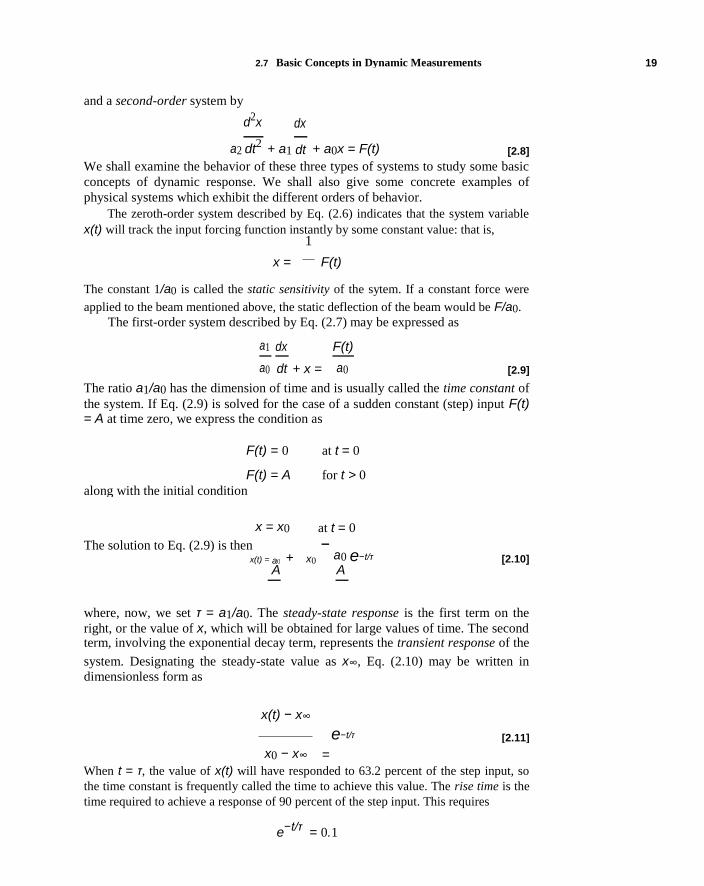
The ratio of output to input amplitude x0/(F0/ k), where x0 is the amplitude of the motion given by

x0 =

F0/ k

[2.25] {[1 − (ω1/ωn)2]2 + [2(c/cc )(ω1/ωn)]2}1/2

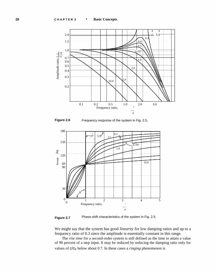
is plotted in Fig. 2.6 to show the frequency response of the system, and the phase

angle φ is plotted in Fig. 2.7 to illustrate the phase-shift characteristics. From these

graphs we make the following observations:

1 − (ω1/ωn)2

For low values of c/cc the amplitude is very nearly constant up to a frequency ratio of about 0.3.

For large values of c/cc (overdamped systems) the amplitude is reduced substan-tially.

The phase-shift characteristics are a strong function of the damping ratio for all

frequencies.


0 /k

0

x F

Am

pli

tude

rati

o,

2.0 1.5

1.0

0.7 0.6 0.5 0.4 0.3

0.2

c 5 0 c

0.3 c

0.4 0.5

0.707

1.0

2.0

10.0 5.0

Figure 2.6

180

150

,deg

120

Phas

eang

le

60 90

30

0

0

Figure 2.7

0.1 0.2 0.5 1.0 2.0 3.0

Frequency ratio, 1

n

Frequency response of the system in Fig. 2.5.

c

5 0 0.5

c 0.3

c

0.707

1.0

10.0

0

1 2 3 4 5

Frequency ratio, 1

n

Phase-shift characteristics of the system in Fig. 2.5.

We might say that the system has good linearity for low damping ratios and up to a

frequency ratio of 0.3 since the amplitude is essentially constant in this range. The rise time for a second-order system is still defined as the time to attain a value

of 90 percent of a step input. It may be reduced by reducing the damping ratio only for

values of c/cc below about 0.7. In these cases a ringing phenomenon is

Inpu

t

Ou

tpu

t

Figure 2.8


Step input

Time

Output response

Rise time Time

Effect of rise time and ringing on output response to a step input.

experienced having a frequency of

ωr = ωn[1 − (c/cc )2]1/2

[2.26]

The rise time and ringing are illustrated in Fig. 2.8. The response time is usually

stated as the time for the system to settle to within ±10 percent of the steady-state

value. The damping characteristics of a second-order system may be studied by

examining the solutions for Eq. (2.20) for the case of a step input instead of the

harmonic forcing function. With the initial conditions

x = 0 at t = 0 dx

= 0 at t = 0

dt

four solution forms may be obtained. Using the nomenclature

and ζ = c/cc

we obtain: x = xs as t → ∞

For ζ = 0, x(t)

= 1 − cos(ωnt)

xs

For 0 < ζ < 1, (1 − ζ2)1/2

sin[ωnt(1 − ζ2)1/2 ]

xs = 1 − exp(−ζωnt) ×

x(t) ζ

cos [ωnt(1 − ζ2)1/2]

[2.27]

[2.28]


x(t)

/xs

2

0

c/cc

0.1 0.2

0.4

0.5

1

1.0 1.5

0 0 2 4 6 8 10

nt

(a)

0

0.1

0.2 2

0.4 x (t)/xs

c/cc

0.5 0

1.0 20

16 12

1.5 8

4

0 nt

(b)

Figure 2.9 (a) Response of second-order system to step input. (b) Three-dimensional

representation of second-order system response to step input.


For ζ = 1,

x(t)

= 1 − (1 + ωnt) exp(−ωnt)

[2.29]

xs

For ζ > 1,

x(t) 1 ζ + K exp( ζ Kω t) ζ − K exp( ζ Kω t) [2.30]

xs =

− 2K × − + − 2K × − −

n n where K = (ζ2

− 1)1/2.

We note that xs is the steady-state displacement obtained after a long period of time. A plot of these equations is shown in Fig. 2.9a for several values of the damping ratio. We observe that:

For an undamped system (c = 0, ζ = 0) the initial disturbance produces a

harmonic response which continues indefinitely. For an underdamped system (ζ < 1) the displacement response overshoots the

steady-state value initially, and then eventually decays to the value of xs. The smaller the value of ζ, the larger the overshoot.

For critical damping (ζ = 1, c = cc ) an exponential rise occurs to approach the steady-state value without overshoot.

For overdamping (ζ > 1) the system also approaches the steady-state value

with-out overshoot, but at a slower rate.

The damping action of Fig. 2.9a is shown over double the number of cycles in

the three-dimensional format of Fig. 2.9b. The latter format illustrates perhaps

more graphically the contrast between harmonic behavior for underdamped

systems and exponential approach to steady state for the overdamped situation. While this brief discussion has been concerned with a simple mechanical

system, we may remark that similar frequency and phase-shift characteristics are

exhibited by electrical and thermal systems as well, and whenever time-varying

measurements are made, due consideration must be given to these characteristics.

Ideally, we should like to have a system with a linear frequency response over all

ranges and with zero phase shift, but this is never completely attainable, although a

certain instrument may be linear over a range of operation in which we are

interested so that the be-havior is good enough for the purposes intended. There are

methods of providing compensation for the adverse frequency-response

characteristics of an instrument, but these methods represent an extensive subject in

themselves and cannot be dis-cussed here. We shall have something to say about

the dynamic characteristics of specific instruments in subsequent chapters. For

electrical systems and recording of dynamic signals digital methods can eliminate

most adverse frequency-response problems.


Example 2.4 SELECTION OF SECOND-ORDER SYSTEM. A second-order system is to be subjected

to inputs below 75 Hz and is to operate with an amplitude response of ±10 percent. Select appropriate design parameters to accomplish this goal.

Solution

The problem statement implies that the amplitude ratio x0 k/F must remain between 0.9 and

1.10. There are many combinations of parameters which can be used. Examining Fig. 2.6, we

see that the curve for c/cc = 0.707 has a flat behavior and drops off at higher frequencies. If

we take the ordinate value of 1.0 as the mean value, then the maximum frequency limit will be

obtained from Eq. (2.25), where

1

0.9 =

{[1 − (ω1 /ωn )

2 ]

2 + [2(c/cc )(ω1 /ωn )]

2 }

1/2

This requires that

ω1

= 0.696 ω

n

We want to use the system up to 75 Hz = 471 rad/s so that the minimum value of ωn is 471

= 677 rad/s

ωn (min) =

0.696

Example 2.5 RESPONSE OF PRESSURE TRANSDUCER. A certain pressure transducer has a natural

frequency of 5000 Hz and a damping ratio c/cc of 0.4. Estimate the resonance frequency and amplitude response and phase shift at a frequency of 2000 Hz.

Solution We have

ωn = 5000 Hz c/cc = 0.4

From Fig. 2.6 we estimate that the maximum amplitude point for these conditions occurs at

ω1

∼ 0.8

So, ω1 ∼ (0.8)(5000) = 4000 Hz for resonance. At 2000 Hz we obtain

ω1=

2000 = 0.4 ωn 5000

which may be inserted into Eq. (2.23) to give the phase shift as

= −tan−1(2)(0.4)(0.4) 1

− (0.4)2 −20.9◦ = −0.364 rad

2.8 System Response 31

The amplitude ratio is obtained from Eq. (2.15) as x0

=

1

F0 / k {[1 − (0.4)2 ]

2 + [(2)(0.4)(0.4)]

2 }

1/2

1.112 The dynamic error in this case would be

1.112 − 1 = 0.112 = ±11.2%

RISE TIME FOR DIFFERENT NATURAL FREQUENCIES. Determine the rise time for Example 2.6 a critically damped second-order system subjected to a step input when the natural frequency

of the system is (a) 10 Hz, (b) 100 kHz, (c) 50 MHz.

Solution We have the natural frequencies of

ωn = 10 Hz = 62.832 rad/s

ωn = 100 kHz = 6.2832 × 105 rad/s

ωn = 50 MHz = 3.1416 × 108 rad/s

For a critically damped system subjected to a step input, ζ = c/cc = 1.0 and Eq. (2.29) applies

x(t)/xs = 1 − (1 + ωn t) exp(−ωn t) [a]

The rise time is obtained when x(t)/xs = 0.9 so that Eq. (a) becomes

0.1 = (1 + ωn t) exp(−ωn t) [b] which has the solution

ωn t = 3.8901 Solving for the rise time at each of the given natural frequencies

trise = 3.8901/ωn

t10 Hz = 0.06191 s

t100 kHz = 6.191 μs t

50 MHz = 0.01238 μs

2.8 System Response

We have already discussed the meaning of frequency response and observed that in

order for a system to have good response, it must treat all frequencies the same

within the range of application so that the ratio of output-to-input amplitude

remains the same over the frequency range desired. We say that the system has

linear frequency response if it follows this behavior.


Amplitude response pertains to the ability of the system to react in a linear way

to various input amplitudes. In order for the system to have linear amplitude

response, the ratio of output-to-input amplitude should remain constant over some

specified range of input amplitudes. When this linear range is exceeded, the system

is said to be overdriven, as in the case of a voltage amplifier where too high an

input voltage is used. Overdriving may occur with both analog and digital systems. We have already noted the significance of phase-shift response and its relation

to frequency response. Phase shift is particularly important where complex

waveforms are concerned because severe distortion may result if the system has

poor phase-shift response.

2.9 Distortion

Suppose a harmonic function of a complicated nature, that is, composed of many

frequencies, is transmitted through the mechanical system of Figs. 2.4 and 2.5. If

the frequency spectrum of the incoming waveform were sufficiently broad, there

would be different amplitude and phase-shift characteristics for each of the input-

frequency components, and the output waveform might bear little resemblance to

the input. Thus, as a result of the frequency-response characteristics of the system,

distortion in the waveform would be experienced. Distortion is a very general term

that may be used to describe the variation of a signal from its true form. Depend-

ing on the system, the distortion may result from either poor frequency response or

poor phase-shift response. In electronic devices various circuits are employed to re-

duce distortion to very small values. For pure electrical measurements distortion is

easily controlled by analog or digital means. For mechanical systems the dynamic

response characteristics are not as easily controlled and remain a subject for further

development. For example, the process of sound recording may involve very so-

phisticated methods to eliminate distortion in the electronic signal processing; how-

ever at the origin of the recording process, complex room acoustics and

microphone placement can alter the reproduction process beyond the capabilities of

electronic correction. Finally, at the terminal stage, the loudspeaker and its

interaction with the room acoustics can introduce distortions and unwanted effects.

The effects of poor frequency and phase-shift response on a complex waveform are

illustrated in Fig. 2.10.

2.10 Impedance Matching

In many experimental setups it is necessary to connect various items of electrical

equipment in order to perform the overall measurement objective. When connections

are made between electrical devices, proper care must be taken to avoid impedance

2.10 Impedance Matching 33

Phase distorted Frequency distorted True signal

Sig

nal

am

pli

tude

0 60 120 180 240 300 360

Harmonic angle, deg

Figure 2.10 Effects of frequency response and phase-shift response on

complex waveform.

mismatching. The input impedance of a two-terminal device may be illustrated as in

Fig. 2.11. The device behaves as if the internal resistance Ri were connected in series

with the internal voltage source E. The connecting terminals for the instrument are

designated as A and B, and the open-circuit voltage presented at these terminals is the

internal voltage E. Now, if an external load R is connected to the device and the

internal voltage E remains constant, the voltage presented at the output terminals A and

B will be dependent on the value of R. The potential presented at the output

Load

E A A

Ri

E R

B R

iB

Figure 2.11 Two-terminal device with internal impedance Ri.


terminals is R

EAB = E [2.31]

R + Ri

The larger the value of R, the more closely the terminal voltage approaches the in-

ternal voltage E. Thus, if the device is used as a voltage source with some internal

impedance, the external impedance (or load) should be large enough that the volt-

age is essentially preserved at the terminals. Or, if we wish to measure the internal

voltage E, the impedance of the measuring device connected to the terminals

should be large compared with the internal impedance. Now, suppose that we wish to deliver power from the device to the external

load R. The power is given by

E2 P = AB [2.32]

R

We ask for the value of the external load that will give the maximum power for a

constant internal voltage E and internal impedance Ri. Equation (2.32) is rewritten E2 2 R

P =

[2.33] R R R

and the maximizing condition + i

dP

= 0

[2.34]

dR

is applied. There results

R = Ri [2.35]

That is, the maximum amount of power may be drawn from the device when the

impedance of the external load just matches the internal impedance. This is the es-

sential principle of impedance matching in electric circuits.

Example 2.7 POWER SUPPLY. A power supply has an internal impedance of 10 and an internal

voltage of 50 V. Calculate the power which will be delivered to external loads of 5 and 20 .

Solution

For this problem we apply Eq. (2.33) with E = 50 V, Ri = 10 , and R = 5 or 20 .

R = 5 : P = (50)2 5 2

= 55.55 W 5 15

R = 15 : P = (50)2 15 2 = 60.0 W 15 25

For maximum power delivery R = Ri and

Pmax = 62.5 W

2.11 Fourier Analysis 35

Clearly, the internal impedance and external load of a complicated electronic

device may contain inductive and capacitative components that will be important in

alternating current transmission and dissipation. Nevertheless, the basic idea is the

same. The general principles of matching, then, are that the external impedance

should match the internal impedance for maximum energy transmission (minimum

attenuation), and the external impedance should be large compared with the inter-

nal impedance when a measurement of internal voltage of the device is desired. It

is this latter principle that makes an electronic voltmeter essential for measurement

of voltages in electronic circuits. The electronic voltmeter has a very high internal

impedance so that little current is drawn and the voltage presented to the terminals

of the instrument is not altered appreciably by the measurement process. Many

such voltmeters today operate on digital principles but all have the capacity of very

high-input impedance. Impedance-matching problems are usually encountered in electrical systems

but can be important in mechanical systems as well. We might imagine the simple

spring-mass system of the previous section as a mechanical transmission system.

From the curves describing the system behavior it is seen that frequencies below a

certain value are transmitted through the system; that is, the force is converted to

displacement with little attenuation. Near the natural frequency undesirable ampli-

fication of the signal is performed, and above this frequency severe attenuation is

present. We might say that this system exhibits a behavior characteristic of a vari-

able impedance that is frequency-dependent. When it is desired to transmit

mechan-ical motion through a system, the natural-frequency and dampling

characteristics must be taken into account so that good “matching” is present. The

problem is an impedance-matching situation, although it is usually treated as a

subject in mechanical vibrations.

2.11 Fourier Analysis

In the early 19th century Joseph Fourier introduced the notion that a piecewise con-

tinuous function that is periodic may be represented by a series of sine and cosine

functions [19]. Thus

y(x) = a0 + a1cos x + a2cos 2x + · · · + ancos nx

+b1sin x + b2sin 2x + · · · + bnsin nx or, more compactly,

∞

y(x) =

a0 + n 1 (ancos nx + bnsin nx) [2.36]

=

The values of the constants a0, an, and bn may be determined by integrating Eq.

(2.36) over the period from −π < x < π.


First,

π

y(x)dx = 2πa0 + 0 + 0 = 2πa0 −π

since the integrals of the sine and cosine functions over the interval −π to π are both zero. We thus have,

a0 = (1/2π) π y(x)dx [2.37]

−π

To determine bn we multiply both sides of Eq. (2.36) by sin mx where m is an integer that may or may not be equal to the summation index n. We have

π

sin mxdx = 0 −π

π cos nxsin mxdx = 0 for m = n

−π π

bnsin2nxdx = πbn for m = n

−π so that,

bn = (1/π) π y(x)sin nxdx [2.38]

−π

In a similar manner, we can determine the coefficients an by multiplying Eq. (2.36) by cos mx and integrating over the interval. This results in

an = (1/π) π y(x)cos nx dx [2.39]

−π Note that when y(x) is an even function, that is, f(x) = f(−x), the function is

represented by cosines alone, and if the function is odd, that is, f(x) = −f(−x), it is

represented by sines alone. If the function is neither even nor odd, all terms must

be employed. The interval for expansion of the function may be expressed in a more general

sense by making a variable substitution. Let

u = (π/L)x [2.40]

Then the coefficients an and bn become

an = (1/L) L y(x) cos (nπx/L) dx [2.41] −L

bn = (1/L) L y(x) sin (nπx/L) dx [2.42] −L

a0 = (1/2L) L y(x) dx [2.43]

−L


If the function repeats over a period T , then L becomes the half period. The

Fourier representation may be further generalized by replacing the integral limits in

Eqs. (2.41), (2.42), (2.43) by p and p + T where p is an arbitrary value for the start

of the repeating function. Of course, one may just consider that a single sample is

taken and obtain the function over the range T . Fourier series representations of functions are useful in experimental measure-

ments in those applications where oscillatory phenomena are observed, as for the

vibrating spring mass of Fig. 2.4, in a resonant electric circuit, or in applications

concerned with propagation of sound waves and their absorption. The measurement

that is usually made is one of the amplitude of vibration as a function of time. The

independent variable in the Fourier series would then be time. We may rearrange the

Fourier series in terms of a circular frequency ω related to the period T through

ω = 2π/T = 2πf [2.44]

where ω is expressed in radian/sec and f is expressed in cycles/sec or Hertz. The summation index n is then said to determine the harmonics of the wave: n

= 1 represents the fundamental value or the lowest frequency, n = 2 the second

harmonic, n = 3 the third harmonic, and so on. We may also introduce the concept of the phase angle presented in Eq. (2.14)

to combine the sine and cosine terms into the following form

∞

y(t) =

a0 + n 1 (an cos nωt + bn sin nωt)

=

∞

= a

0 + n 1 Cn cos (nωt − φn) [2.45]

=

where the new constant Cn is determined from

Cn = (an2 + bn

2)1/2 [2.46]

and the phase angle is determined from

tan φn = bn/an [2.47]

If one were to apply Eqs. (2.41), (2.42), and (2.43) for the constants a0, an, and bn to the trigonometric function

y(x) = 3.5 + 2 sin x + 6.3 cox 5x the simple result

a0 = 3.5

an = 2 for n = 1

0 for n =1

bn = 6.3 for n = 5 = 0 for n =5

would be obtained.

38 C H A P T E R 2 •Basic Concepts

y(x) y(x) y(x)

A

A

A

x x x

W W W

(a) (b) (c)

Figure 2.12 (a) Square wave function. (b) Sawtooth function. (c) Ramp function.

Now let us consider three waveforms as examples of Fourier series. In Fig.

2.12 we have (a) a square wave of amplitude A and width W , (b) a sawtooth wave

of amplitude A and width W , and (c) a ramp function having amplitude A and

duration W . In an experiment the amplitude might be displacement in a

mechanical system, voltage in an electric circuit, or sound pressure level in an

acoustic system. The duration of the wave would be some unit of time. The square wave is described by

y(x) = A for 0 < x < W [2.48]

= 0 for x < 0

= 0 for x > W

Later we will substitute ωt for the displacement function x. This is an odd function

so we expect only sine terms in the series. Inserting the constant amplitude in Eq.

(2.42) we obtain

bn = (2A/nπ)[1 − cos(nπx/W)] [2.49]

which reduces to

bn = 4A/nπ for n = odd [2.50]

= 0 for n = even The final series representation for the square wave is thus

∞

{[(−1)n+1 + 1]/n}sin(nπx/W)

y(x) = (2A/π) n 1 [2.51]

= This series may be summed as indicated or an alternate index, which automatically leaves out the zero terms, may be used to obtain

∞

1

[sin(2N − 1)πx/W ]/(2N − 1) [2.52] y(x) = (4A/π) N=

Note that the index n, and not N, represents the harmonics: n = 1 (N = 1) represents the fundamental, n = 3 (N = 2) represents the third harmonic, n = 5 (N = 3) represents the fifth harmonic, and so on.


Figure 2.13 shows the summation represented by Eq. (2.52) for N = 1 to 50 (n

= 1 to 99). In Fig. 2.13a the lines become quite cluttered, but are shown more

clearly in Fig. 2.13b. A three-dimensional diagram is shown in Fig. 2.13c that

illustrates how the bumps in the square wave are smoothed out as the number of

terms in the series is increased. Now, let us examine the other two cases in Fig. 2.12. The sawtooth wave is described by

y(x) = (2A/W)x for 0 < x < W/2 [2.53a]

= −(2A/W)x + 2A for W/2 < x < W [2.53b]

Applying Eq. (2.43) for the Fourier coefficient a0 as before gives

W W

a0 = (4/W) (2A/W)xdx + [(−2A/W)x + 2A]dx = A/2 [2.54] 0 0

1.4

1.2

1

0.8

y(x)

/A

0.6

0.4

0.2

0

0 0.1 0.2 0.3 0.4 0.5 0.6 0.7 0.8 0.9 1 x/W

(a)

Figure 2.13 (a) Square wave for n = 1 to 99; (b) Square wave for five values of

index n; (c) Three-dimensional view of square wave Fourier series.


1.4

1.2

1

0.8 n =

/ A

y ( x ) 1

9

0.6 19

59

99

0.4

0.2

0 0.4 0.6 0.8 0 0.2

x/W (b)

n = 99 1.4

1.2

n = 59 1 0.8

n = 19 0.6 0.4

0.2

n = 9 0

n = 1 x/W

1

/A y(x)

(c)

Figure 2.13 (Continued)


Using Eq. (2.41) for an and Eq. (2.42) for bn results in

an = (2A/n2π2)(cos nπ − 1) [2.55]

= 0 for n even

= −(4A/n2π2) for n odd [2.56] and

bn = 0 Making the same index substitution as before to automatically omit the zero terms gives for the final series

ω 1

cos[(2N − 1)2πx/W ]/(2N − 1)2

y(x) = A/2 − (4A/π2) [2.57]

N=

For the ramp function shown in Fig. 2.13c the Fourier series becomes

ω

y(x) = (2A/π) n 1 (−1)n+1[sin(nπx/W)]/n [2.58]

= The index n in this series does represent the harmonics. Equations (2.57) and (2.58) are plotted in Figs. 2.14 and 2.15.

y(x)

/A

1.2

1

0.8

0.6

0.4

0.2

0

0 0.1 0.2 0.3 0.4 0.5 0.6 0.7 0.8 0.9 1 x/W

(a)

Figure 2.14 (a) Fourier representation for Sawtooth for n = 1 to 30;

(b) Three-dimensional representation for sawtooth n = 1 to 30.


1

0.5

0

(b)


The Decibel

As we shall see in later sections, one is frequently interested in the value of a cer-

tain parameter as related to a reference value of that parameter. The electric power

dissipated in a resistor is

P = E2/R


y(x)

/A

1.2

1

0.8

0.6

0.4

0.2

0

0 0.1 0.2 0.3 0.4 0.5 0.6 0.7 0.8 0.9 1 x/W

(a)

1.2 1 0.8 0.6 0.4 0.2 0

0.82

0.62

0.42

0.22

0.02 (b)

Figure 2.15 (a) Ramp function; (b) Three-dimensional representation of ramp function.


The decibel is defined in terms of some reference Power Pref as

decibel = dB = 10 log(P/Pref) [2.59]

In terms of the voltage the decibel level would be

dB = 20 log(E/Eref) [2.60]

since the power varies as the square of the voltage.

If we identify the square wave of Fig. 2.13 with a voltage pulse and the Fourier

series as a representation of that pulse over a certain frequency range, we could express

the accuracy of the representation in terms of decibel units by choosing the reference

value as [y(x)]ref = 1.0. Then the decibel response would appear as in Fig. 2.16. We

could say that the square wave is faithfully reproduced within

±0.4 dB for a frequency response up to the 99th harmonic

±0.6 dB for a frequency response up to the 59th harmonic ±1.4 dB for a frequency response up to the 19th harmonic ±4.1 dB for a frequency response up to the 9th harmonic.

All of these values are within the range 0.02 < x/W < 0.98. This means that an electronic amplifier to reproduce step or square wave pulse

functions must have frequency-response capabilities that far exceed the

fundamental frequency of the basic wave.

2

0

–2

)

r e f

y/y

–4

= 1

0lo

g(

–6

dB

–8

–10

–12 0 0.2 0.4 0.6 0.8 1

x/W

Figure 2.16 Decibel representation of square wave.

n559 n599 n519

n59


The Fourier Transform We have already noted that a Fourier series representation of a function breaks

down the function into harmonic components. For the case of the square wave the

Fourier coefficients are shown in Fig. 2.17 as a function of the harmonic index n.

Thus, an os-cillatory displacement behavior of a spring-mass damper system could

be represented as a summation of frequency components. Or, we might say that the

physical represen-tation in the displacement-time domain could be transformed

into a frequency-time domain through the use of Fourier series. In practice, a signal may be sampled in discrete time increments t and stored in

a digital computer. If N increments in t are taken over the signal, the period T

becomes

T = N t To evaluate the integrals in Eqs. (2.41), (2.42), and (2.43) the integration must be performed numerically.

The signal is y(tk ) where k is a new index indicating the time increment so that

tk = k t for k = 1, 2, · · · , N [2.61]

1.4

1.2

1

/A

0.8 n

b

0.6

0.4

0.2

0 0 10 20 30 40 50

N = (n + 1)/2

Figure 2.17 Fourier coefficients for square wave.


The Fourier coefficients thus are expressed in terms of summations instead of

integrals to give

N

an =

(2/N) k 1 y(k t)cos(2πkn/N) for n = 0 to N/2 [2.62]

= N

bn =

(2/N) k 1 y(k t)sin(2πkn/N) for n = 1 to N/2 − 1 [2.63]

= where N, the number of time increments, is selected as an even number.

The coefficient ao is obtained by performing a numerical integration of the dis-crete function by the most appropriate method. (See Sect. 5.8.)

The operations performed in the foregoing summations are called a Discrete

Fourier transform (DFT) and may be performed either with separate software pack-

ages or with built-in computation algorithms in the particular device employed for the

data collection. Hardware dedicated to specific applications may have integrated

circuits that output information in the exact format needed by the user. As the number of samples increases, the number of computations required for the

discrete Fourier transform increases by N2. The fast Fourier transform (FFT) employs

a special algorithm to speed the calculation for large data samples so that the number of

computations varies as N log2 N instead of N2. For samples with N about 1000 the FFT

is about 100 times faster than the DFT scheme. The reader may consult Refs. [19], [20],

[21] for further information on the development of the DFT and FFT, and Ref. [22] for

specific calculation techniques and examples. In Sect. 14.5 we shall see that it is

necessary to sample at a frequency at least twice the anticipated frequency content of

the signal to avoid the problem of aliasing. The highest frequency that may be resolved

is called the Nyquist frequency and is given by

fNyq = fs/2 = 1/2 t [2.64]

where fs is the sampling frequency and t, as before, is the sampling time increment.

2.12 Experiment Planning

The key to success in experimental work is to ask continually: What am I looking

for? Why am I measuring this—does the measurement really answer any of my

questions? What does the measurement tell me? These questions may seem rather

elementary, but they should be asked frequently throughout the progress of any

experimental program. Some particular questions that should be asked in the initial

phases of experiment planning are:

What primary variables shall be investigated?

What control must be exerted on the experiment?

What ranges of the primary variables will be necessary to describe the

phenom-ena under study?

2.12 Experiment Planning 47

How many data points should be taken in the various ranges of operation to

ensure good sampling of data considering instrument accuracy and other

factors? (See Chap. 3.)

What instrument accuracy is required for each measurement?

If a dynamic measurement is involved, what frequency response must the in-

struments have?

Are the instruments available commercially, or must they be constructed espe-

cially for the particular experiment?

What safety precautions are necessary if some kind of hazardous operation is

involved in the experiment?

What financial resources are available to perform the experiment, and how do

the various instrument requirements fit into the proposed budget? What provisions have been made for recording the data?

What provisions have been made for either on-line or subsequent computer

reduction of data? If the data reduction is not of a “research” nature where manipulation and calcu-

lations depend somewhat on the results of measurements, what provisions are

made to have direct output of a data acquisition system available for the final

report? In many cases appropriate graphical results may be obtained with digital

data acquisition systems as the experiment progresses or shortly thereafter.

The importance of control in any experiment should always be recognized.

The physical principle, apparatus, or device under investigation will dictate the

variables which must be controlled carefully. For example, a heat-transfer test of a

particu-lar apparatus might involve some heat loss to the surrounding air in the

laboratory where the test equipment is located. Consequently, it would be wise to

maintain (con-trol) the surrounding temperature at a reasonably constant value. If

one run is made with the room temperature at 90◦C and another at 50

◦F, large

unwanted effects may occur in the measurements. Or, suppose a test is to be made

of the effect of cigarette smoke on the eating habits of mice. Clearly, we would

want to control the con-centration of smoke inhaled by the mice and also observe

another group of mice which were not exposed to cigarette smoke at all. All other

environmental variables should be the same if we are to establish the effect of the

cigarette smoke on eating habits. In the case of the heat-transfer test we make a series of measurements of the char-

acteristics of a device under certain specified operating conditions—no comparison

with other devices is made. For the smoke test with mice it is necessary to measure the

performance of the mice under specified conditions and also to compare this perfor-

mance with the performance of another group under different controlled conditions. For

the heat-transfer test we establish an absolute measurement of performance, but for the

mice a relative performance is all that can be ascertained. We have chosen two diverse

examples of absolute and relative experiments, but the lesson is clear. Whenever a

comparison test is performed to establish relative performance, control


must be exerted over more than one experimental setup in order for the comparison

to be significant. It would seem obvious that very careful provisions should be made to record the

data and all ideas and observations concerned with the experiment. Yet, many experi-

menters record data and important sketches on pieces of scratch paper or in such a dis-

organized manner that they may be lost or thrown away. In some experiments the read-

out instrument is a recording type so that a record is automatically obtained and there is

little chance for loss. For many experiments, however, visual observations must be

made and values recorded on an appropriate data sheet. This data sheet should be very

carefully planned so that it may subsequently be used, if desired, for data reduction.

Frequently, much time may be saved in the reduction process by eliminating unnec-

essary transferal of data from one sheet to another. If a computer is to be used for data

reduction, then the primary data sheet should be so designed that the data may be eas-

ily transferred to the input device of the computer. Even with digital readout systems

the printout must be carefully labeled, either in the machine programming or by hand. A bound notebook should be maintained to record sketches and significant

observations of an unusual character which may occur during both the planning and

the execution stages of the experiment. The notebook is also used for recording

thoughts and observations of a theoretical nature as the experiment progresses. Upon

the completion of the experimental program the well-kept notebook forms a clear and

sequential record of the experiment planning, observations during the experiment, and,

where applicable, correspondence of important observations with theoretical

predictions. Every experimenter should get into the habit of keeping a good notebook.

In some cases the output of various instrument transducers will be fed directly to a data

acquisition system and computer which processes the data and furnishes a printed

output of the desired results. Then, the notebook becomes the repository of important

sketches and listings of computer programs, as well as documentation which may be

needed later to analyze the data or repeat the experiment. Sample printouts or

computer-generated graphs may be taped in the notebook along with program

documentation. For those engineers conducting tests or experiments that are an essential part of

product development, which may lead to patent application, the bound notebook is an

essential legal element in the documentation that may be required in securing and

defending the patent. The well-documented bound notebook is an obvious advantage to

the person(s) who may be called upon to continue the work. One may suggest that

computer records and documentation substitute for the notebook and offer the ability

for rapid transfer of information to other interested parties. For confidential informa-

tion the need for stringent security measures in any electronic transmission is obvious. As a summary of our remarks on experimental planning we present the gen-

eralized experimental procedure given in Table 2.8. This procedure is, of course, a

flexible one, and the reader should consider the importance of each item in relation to

the entire experimental program. Notice particularly item 1a. The engineer should give

careful thought to the need for the experiment. Perhaps after some sober thinking the

engineer will decide that a previously planned experiment is really not necessary at all

and that the desired information could be found from an analytical study or from

2.12 Experiment Planning 49

Table 2.8 Generalized experimental procedure

a. Establish the need for the experiment.

b. Establish the optimum budgetary, manpower, and time requirements, including time

sequencing of the project. Modify scope of the experiment to actual budget, manpower,

and time schedule which are allowable. Begin detail planning for the experiment; clearly establish objectives of experiment (verify

performance of production model, verify theoretical analysis of particular physical

phenomenon, etc.). If experiments are similar to those of previous investigators, be sure to

make use of experience of the previous workers. Never overlook the possibility that the

work may have been done before and reported in the literature. Continue planning by performing the following steps:

a. Establish the primary variables which must be measured (force, strain, flow, pressure,

temperature, etc.). b. Determine as nearly as possible the accuracy which may be required in the primary

measurements and the number of such measurements which will be required for proper

data analysis. c. Set up date reduction calculations before conducting the experiments to be sure that

adequate data are being collected to meet the objectives of the experiment. d. Analyze the possible errors in the anticipated results before the experiments are conducted

so that modifications in accuracy requirements on the various measurements may be

changed if necessary. Select instrumentation for the various measurements to match the anticipated accuracy

requirements. Modify the instrumentation to match budgetary limitations if necessary.

Collect a few data points and conduct a preliminary analysis of these data to be sure that the

experiment is going as planned. Modify the experimental apparatus and/or procedure in accordance with the findings in item 5. Collect the bulk of experimental data and analyze the results. Organize, discuss, and publish the findings and results of the experiments, being sure to include

information pertaining to all items 1 to 7, above.

the results of experiments already conducted. Do not take this item lightly. A great

amount of money is wasted by individuals who rush into a program only to discover

later that the experiments were unnecessary for their own particular purposes.

The Role of Uncertainty Analysis in Experiment Planning Items 3b and d in Table 2.8 note the need to perform preliminary analyses of

experi-mental uncertainties in order to effect a proper selection of instruments and

to design the apparatus to meet the overall goals of the experiment. These items are

worthy of further amplification. Recall our previous comments about the terms accuracy, error, and uncertainty.

We noted that many persons use the term “error” when “uncertainty” is the proper

nomenclature. As promised before, we shall clarify this matter in Chap. 3. In Chap. 3 we shall see how one goes about estimating uncertainty in an ex-

perimental measurement. For now, let us consider how these estimates can aid our

experiment planning. It is clear that certain variables we wish to measure are set by

the particular experimental objectives, but there may be several choices open in the


method we use to measure these variables. An electric-power measurement could be

performed by measuring current and voltage and taking the product of these variables.

The power might also be calculated by measuring the voltage drop across a known re-

sistor, or possibly through some calorimetric determination of the heat dissipated from

a resistor. The choice of the method used can be made on the basis of an uncertainty

analysis, which indicates the relative accuracy of each method. A flow measurement

might be performed by sensing the pressure drop across an obstruction meter, or possi-

bly by counting the number of revolutions of a turbine placed in the flow (see Chap. 7).

In the first case the overall uncertainty depends on the accuracy of a measurement of

pressure differential and other variables, such as flow area, while in the second case the

overall uncertainty depends on the accuracy of counting and a time determination. The point is that a careful uncertainty analysis during the experiment planning

period may enable the investigator to make a better selection of instruments for the

program. Briefly, then, an uncertainty analysis enters into the planning phase with

the following approximate steps:

Several alternative measurement techniques are selected once the variables to

be measured have been established.

An uncertainty analysis is performed on each measurement technique, taking

into account the estimated accuracies of the instruments that will actually be

used.

The different measurement techniques are then compared on the basis of cost,

availability of instrumentation, ease of data collection, and calculated uncer-

tainty. The technique with the least uncertainty is clearly the most desirable

from an experimental-accuracy standpoint, but it may be too expensive. Fre-

quently, however, the investigator will find the cost is not a strong factor and

that the technique with the smallest uncertainty (within reason) is as easy to

perform as some other less accurate method.

Figure 2.18 divides the procedure of Table 2.8 into a graphical pattern of pre-

liminary, intermediate, and final stages of an experimental program. The feedback

blocks in these diagrams are very important because they illustrate the need to

retrace continuously one’s steps and modify the program in accordance with the

most current information that is available. In Chap. 16 we will return to the notions of experiment planning by examining

a reasonable design protocol for experiments. This procedure will build upon the

information pertaining to uncertainty analysis contained in Chap. 3, which we have

already mentioned several times, as well as specific measurement techniques

which will be explored in other chapters.

2.13 Review Questions

2.1. What is meant by sensitivity; accuracy; precision?

2.2. Why is instrument calibration necessary?

2.13 Review Questions 51

If not feasible require

Possibly modify modification of budget

scope of analytical and/or time schedule

work

or discontinue effort

Establish

Establish time

Estimate scope

Carefully review Establish general

feasibility within need for

and financial

of accompanying

previous work in

original budget and experiment limitations analytical work the field

time limitations

Possibly modify original notion

of “need”

(a)

Begin preliminary

analytical work in order to:

Determine variable Arrange for design Collect a few Analyze uncertainty ranges and accuracies

and construction of

preliminary data

in data required

special equipment

points

If comparison not

Specify instruments favorable possibly

required modify experiment

and /or analysis

Modify in Proceed with

Compare preliminary accordance with data with theories

analytical work

budget limitations available

Purchase instruments

(b)

Figure 2.18 (a) Preliminary stages of experiment planning; (b) intermediate stages

of experiment planning; (c) final stages of experimental program.


Collect bulk

of data Match theories with experiment, correlate

data, create new theories to explain data, etc.

Continue analysis including possible

computer runs

Correlate with original need

for experiment

(c)


Discuss and

publish results of experiments

2.3. Why are standards necessary?

2.4. What is meant by frequency response?

2.5. Describe the meaning of phase shift.

2.6. Define time constant.

2.7. What kind of impedance matching is desired for (a) maximum power trans-

mission and (b) minimum influence on the output of the system?

2.8. Why is a literature survey important in the preliminary stages of experiment

planning?

2.9. Why is an uncertainty analysis important in the preliminary stages of experi-

ment planning?

2.10. How can an uncertainty analysis help to reduce overall experimental uncer-

tainty?

2.11. What is rise time?

2.12. What is meant by zeroth-, first-, and second-order systems?

2.13. What is meant by steady-state response?

2.14. What factors influence the time constant in first-order systems?

2.14 Problems

2.1. Consider an ordinary mercury-in-glass thermometer as a measurement system and

indicate which parts of the thermometer correspond to the boxes in the diagram of

Fig. 2.2.

2.14 Problems 53

2.2. A thermometer is used for the range of 200 to 400◦F, and it is stated that its

accuracy is one-quarter of 1 percent. What does this mean in terms of temperature?

2.3. A sinusoidal forcing function is impressed on the system in Fig. 2.5. The natural

frequency is 100 Hz, and the damping ratio c/cc is 0.7. Calculate the amplitude

ratio and time lag of the system for an input frequency of 40 Hz. (The time lag is

the time interval between the maximum force input and maximum displacement

output.)

2.4. For a natural frequency of 100 Hz and a damping ratio of 0.7, compute the input-

frequency range for which the system in Fig. 2.5 will have an amplitude ratio of

1.00 ± 0.01.

2.5. A thermometer is initially at a temperature of 70◦F and is suddenly placed in a

liquid which is maintained at 300◦F. The thermometer indicates 200 and 270

◦F

after time intervals of 3 and 5 s, respectively. Estimate the time constant for the thermometer.

2.6. Plot the power output of the circuit in Fig. 2.11 as a function of R/Ri. Assume Ri

and E as constants and show the plot in dimensionless form; that is, use PRi/E2 as

the ordinate for the curve.

2.7. A steel scale is graduated in increments of 321 in. What is the readability and least

count of such a scale? 2.8. A 10-μF capacitor is charged to a potential of 100 V. At time zero it is discharged

through a 1-M resistor. What is the time constant for this sytem? 2.9. The two-terminal device shown in Fig. 2.11 has an internal resistance of 5000 . A

meter with an impedance of 20,000 is connected to the output to perform a

voltage measurement. What is the percent error in determination of the internal

voltage?

2.10. The device in Prob. 2.9 has an internal voltage of 100 V. Calculate the power

output for the loading conditions indicated. What would be the maximum power

output? What power output would result for a load resistance of 1000 ? 2.11. A 2-g mass is suspended from a simple spring. The deflection caused by this mass

is 0.5 cm. What is the natural frequency of the system? 2.12. A 10-lbm turntable is placed on rubber supports such that a deflection of 0.25 in

results from the weight. Calculate the natural frequency of such a system. 2.13. A resistance-capacitance system is to be designed with a time constant of 1 ms.

Specify several combinations of R and C to accomplish this, and based on com-

mercially available items, obtain the cost of each combination. 2.14. What is the minimum amplitude reduction to be expected for the system in Prob.

2.12 for frequencies greater than 20, 40, and 60 Hz?

2.15. A small tank contains 10 liters of water at 20◦C which is allowed to discharge from

an opening in the side at the initial rate of 6 liters/h. The discharge rate is


directly proportional to the volume of water remaining in the tank. Calculate

an equivalent time constant for this system.

2.16. Pressure is measured in units of lbf/in2 in the English system of units. Derive

factors to convert to units of N/m2 (Pa) and kilopond/cm

2.

2.17. One gallon equals 231 in3. Derive a conversion factor to convert automobile fuel

economy from mi/gal to km/liter.

2.18. A unit for viscosity in the English system is lbf · s/ft2. Determine a factor to

convert this to kg/m · s.

2.19. A unit for specific heat in the SI system is kJ/kg · ◦C. Derive a factor to convert this

to Btu/lbm · ◦F, and to kcal/g ·

◦C.

2.20. Derive a factor to convert density from g/m3

to slugs/ft3.

2.21. An English unit for thermal conductivity is Btu/h · ft · ◦F. Derive a factor to convert

to ergs/cm · ◦C.

2.22. A unit of kinematic viscosity in the metric system is the Stoke (St), defined as

1.0 cm2/s. Derive a factor to convert to ft

2/s.

2.23. The SI unit for heat generation is W/m3. Derive a factor to convert to Btu/h · ft

3.

2.24. A unit for dynamic viscosity in the metric system is the poise (P) = 1.0 dyn · s/cm2.

Derive a factor to convert to lbm/h · ft.

2.25. Heat flux may be expressed in units of W/cm2. Derive a factor to convert to Btu/h ·

ft2.

2.26. The universal gas constant has a value of 1545 ft · lbf/lbm mol · ◦R. By applying

appropriate conversion factors, obtain its value in SI units.

2.27. Derive a factor to convert volume flow rate from cm3/s to gal/min.

2.28. How do you convert degrees Kelvin to degrees Rankine?

2.29. A thermometer has a time constant of 10 s and behaves as a first-order system. It is

initially at a temperature 30◦C and then suddenly subjected to a surrounding

temperature of 120◦C. Calculate the 90 percent rise time and the time to attain 99

percent of the steady-state temperature.

2.30. The thermometer in Prob. 2.29 is subjected to a harmonic temperature variation

having an amplitude of 20◦C and a frequency of 0.01 Hz. Determine the phase lag

of the thermometer and the amplitude attenuation. The time constant is still taken as 10 s.

2.31. A pressure transducer operates as a second-order system having a natural fre-

quency of 10,000 Hz. For damping ratios c/cc of 0.3 and 0.4, determine the

resonance frequencies.

2.32. For the transducer in Prob. 2.31, determine the amplitude response and dynamic

error for frequencies of 2000 and 4000 Hz. Also, determine the phase lag for these

frequencies.

2.14 Problems 55

2.33. A second-order system is to be designed for damping the amplitude response by 40 percent for input frequencies from 10 to 50 Hz. Select suitable natural frequencies

and damping ratios c/cc to accomplish this objective.

2.34. A first-order system has a phase shift of −50◦ at a certain frequency. What will be

the phase lag at a frequency of twice this value? What will be the relative amplitude responses at the two frequencies?

2.35. A first-order system is subjected to a harmonic input of 3 Hz. The system has a time

constant of 0.5 s. Calculate the error of the amplitude response and the phase lag.

2.36. A thermometer acting as a first-order system is initially at a temperature of 35◦C

and is then suddenly subjected to a temperature of 110◦C. After 8 s the ther-

mometer indicates a temperature of 75◦C. Calculate the time constant and the 90

percent rise time for the thermometer.

2.37. A first-order system has a time constant of 0.05 s. Over what frequency range will

the amplitude response be within 10 percent?

2.38. A force transducer is connected such that the output registers a static sensitivity of

1.0 V/kgf input. What is the output for a force input of 10 kgf?

2.39. The rise time for a certain RC circuit is to be 0.003 ms. Determine suitable values

of R and C to accomplish this.

2.40. A dynamic measurement device operating as a second-order system is to be de-

signed to measure an input frequency of 60 Hz with an amplitude error of no

greater than 5 percent. Determine appropriate design parameters which would

accomplish this objective. Many answers are possible, so discuss what factors

influenced your selection.

2.41. A pressure transducer has a damping ratio of 0.3 and a natural frequency of 12,000

Hz. Determine the frequency range for which the amplitude dynamic error will be

less than 10 percent.

2.42. A small temperature sensor operates as a first-order system and is stated to have a

time constant of 0.1 s. If it is initially at a temperature of 100◦C and suddenly

exposed to an environment temperature of l5◦C, how long will it take to indicate a

temperature of 17◦C?

2.43. If the temperature sensor of Prob. 2.42 is exposed to a harmonic temperature

source, for what frequency range will its amplitude response be within 10 per-

cent? What will be the time delay under these circumstances?

2.44. A pressure transducer operating as a second-order system is to be used to measure a signal at 500 Hz. To select the transducer, we shall choose one with a natural

frequency of 1500 Hz. What damping ratio c/cc must be selected so that the

dynamic error of the amplitude response is less than 2 percent?

2.45. An RC electric circuit is to have a rise time of one microsecond (1 μs). Select

appropriate values of R and C to accomplish this objective.


2.46. A large building mass behaves approximately like a first-order system when re-

sponding to a harmonic thermal input. If the harmonic input follows the pattern of

daily heating and cooling, that is, one cycle occurs over a 24-h period, and the time

delay is 2 h, estimate the time constant for the system. Also, estimate how much

the amplitude response decreases at this frequency.

2.47. A platform weighing 1.3 kg (force) is attached to a spring damper system with a

spring constant of 100 N/m. The damper is adjustable. If the damper is adjusted to

the critical value, how long will it take for the system to recover 90 percent of the

displaced value of a step input?

2.48. The system of Prob. 2.47 is subjected to a step input and the damper is adjusted so

that a damping ratio of 0.1 is obtained. Using the results of Fig. 2.9 or the

appropriate equation, estimate the time required for the system to reach the first

maximum point in overshoot.

2.49. Estimate the rise time for the system in Prob. 2.47 for an overdamped condition

with c/cc = 1.5. 2.50. Calculate the relative displacement from steady-state value for the system in Prob.

2.47 at t = 1 s and c = 5.7 kg/s.

2.51. A special oscilloscope used in high-power laser systems is stated to have a rise time

of 1 picosecond for a step input. What does this imply in terms of frequency

response?

2.52. Assume that the weight of a 3000-lb automobile is distributed evenly over the four

wheels and associated spring shock absorber system. Also assume that the springs

will be deflected 1.5 in when the auto is loaded with 1000 lb. What is the natural

frequency of such a system? What is the rise time for critical damping and a step

input to the system?

2.53. A temperature-sensing element is stated to behave as a first-order system with a rise

time of 0.1 s. If the element is initially at a temperature of 20◦C and suddenly

subjected to a temperature of 125◦C, what temperature will the element indicate

after a time of 0.05 s?

2.54. A metric unit for dynamic viscosity is kg/m-s. Determine a conversion factor to

convert to lbf-s/ft2.

2.55. A dimensionless group used in fluid mechanics is the Reynolds number defined as

Re = ρux/μ

where ρ is fluid density, u is velocity, x is a dimension, and μ is the dynamic

viscosity. Determine sets of units for these four parameters in SI and English

systems that will make Re dimensionless.

2.56. A dimensionless group used in free-convection heat-transfer problems is the

Grashof number defined by

gβρ2 Tx

3

Gr = μ2

2.14 Problems 57

where g is the acceleration of gravity, β is rate of change of fluid volume per unit

change in temperature per unit volume, T is a temperature difference, x is a

distance parameter, and μ is the fluid dynamic viscosity having units of N-s/m2 in

the SI system. Determine suitable units for all parameters in the SI system which

will cause Gr to be dimensionless. Repeat for the English system.

2.57. At a certain electronics company the units employed for thermal conductiv-ity are

W-cm/in2-◦F. Determine a factor to convert to the standard SI unit of W/m-

◦C. In

the thermal conductivity parameter ◦C or

◦F represents a tempera-ture difference.

2.58. A temperature measurement device is believed to behave as a first-order system

with a rise time of 0.2. At time zero the device is at a temperature of 45◦C. What

temperature will be indicated by the device 0.1 s after it is suddenly exposed to a

temperature of 100◦C? Assume that the rise time remains constant.

2.59. An empty pickup truck weighs 4500 lbf with the weight distributed about equally to

the four wheels. When the truck is loaded with 1500 lb distributed uniformly to all

four wheels, the suspension springs deflect by 1 in. Calculate the natural frequency

for the system. Assuming a step input, what would be the rise time for the system?

2.60. A pressure transducer is to be selected to measure a varying pressure at a fre-

quency of 400 Hz. The device selected has a natural frequency of 1200 Hz. It is

desired that the dynamic error of the amplitude response of the transducer not

exceed 2 percent. What damping ratio is necessary to achieve this response?

2.61. Determine the Fourier sine series for the function f(x) = x3

for 0 < x < π Ans. x3 =

2 (−1)n+1

{[(nπ)2 − 6]/n

3}sin nx

2.62. The thermal response of buildings behaves approximately as a first-order system

when subjected to a harmonic temperature variation. Without imposition of a

sudden “cold front” a single cycle is executed over a 24-h period. If the time delay

for maximum and minimum points in the temperature wave lags by 1.5 h, calculate

the time constant for the system.

2.63. A thermocouple behaves approximately as a first-order system. The element is

initially at a temperature of 45◦C and suddenly subjected to a temperature of

100◦C. After a period of 6 s the thermocouple indicates a temperature of 70

◦C.

Calculate the 90 percent rise time for the thermocouple.

2.64. Determine the Fourier series for the function f(x) = x for −π < x < π Ans. x = 2

[(−1)n+1/n]sin nx

2.65. A thermocouple has a time constant of 8 s and may be approximated as a first-order

system. If it is initially at a temperature of 40◦C and suddenly exposed to a

surrounding temperature of l00◦C, calculate the 90 percent rise time and the time

to attain 99 percent of the steady-state temperature.

2.66. A certain first-order system is subjected to a harmonic input of 5 Hz, producing a

time constant of 0.6 s. Calculate the error for the amplitude response and the phase

lag.

Solution Manual for Experimental Methods for Engineers 8th ... · 6 C H A P T E R 2 • Basic...

Documents

Transcript of Solution Manual for Experimental Methods for Engineers 8th ... · 6 C H A P T E R 2 • Basic...