Hysteresis in Ferroelectric Material

Created in COMSOL Multiphysics 5.6

Hy s t e r e s i s i n F e r r o e l e c t r i c Ma t e r i a l

This model is licensed under the COMSOL Software License Agreement 5.6.All trademarks are the property of their respective owners. See www.comsol.com/trademarks.

http://www.comsol.com/sla

http://www.comsol.com/trademarks/

Introduction

Ferroelectric materials exhibit nonlinear polarization behavior such as hysteresis and saturation at large applied electric fields. Many piezoelectric materials are ferroelectric. This model analyzes a simple actuator made of a PZT piezoelectric ceramic material, which is subjected to an applied electric field.

Model Definition

In its ferroelectric phase, the material exhibits spontaneous polarization, so that it is constituted of domains with nonzero polarization even at zero applied field. The application of an electric field can rearrange the domains, resulting in a net polarization in the material. At very large electric fields, the polarization saturates, as all ferroelectric domains in the material are aligned along the direction of the applied field. Domain wall interactions can also lead to a significant hysteresis in the polarization.

The Jiles–Atherton hysteresis model for ferroelectric materials is available in COMSOL Multiphysics. It assumes that the total polarization can be represented as a sum of reversible and irreversible parts. The polarization change is computed from the incremental equation

where the reversibility is characterized by the parameter cr, and the anhysteretic polarization is found from the relation

where Ps is the saturation polarization. The effective electric field is given by

(1)

where α is a material parameter called the inter-domain coupling. The polarization shape is characterized by the Langevin function

where a is a material parameter called the domain wall density.

dP crdPan I cr–( )dPirr+=

Pan PsL Eeff( )EeffEeff-------------=

Eeff E αP+=

LEeff

a------------- coth a

Eeff-------------–=

2 | H Y S T E R E S I S I N F E R R O E L E C T R I C M A T E R I A L

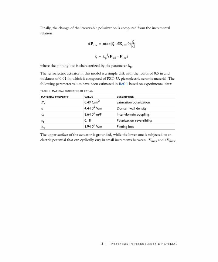
Finally, the change of the irreversible polarization is computed from the incremental relation

where the pinning loss is characterized by the parameter kp.

The ferroelectric actuator in this model is a simple disk with the radius of 0.5 in and thickness of 0.01 in, which is composed of PZT-5A piezoelectric ceramic material. The following parameter values have been estimated in Ref. 1 based on experimental data:

MATERIAL PROPERTY VALUE DESCRIPTION

Ps 0.49 C/m2 Saturation polarization

a 4.4·105 V/m Domain wall density

α 3.6·106 m/F Inter-domain coupling

cr 0.18 Polarization reversibility

kp 1.9·106 V/m Pinning loss

The upper surface of the actuator is grounded, while the lower one is subjected to an electric potential that can cyclically vary in small increments between −Vmax and +Vmax.

TABLE 1: MATERIAL PROPERTIES OF PZT-5A.

dPirr max ζ dEeff 0,⋅( ) ζζ-----=

ζ kp1– Pan Pirr–( )=


The actuator is surrounded by air. Because of the symmetry, it is sufficient to model only the upper half of the setup.

Figure 1: Model geometry. The smaller domain represents the upper half of the ferroelectric actuator. The larger domain is used for modeling the surrounding air.


Because of the actuator aspect ratio, a relatively coarse mesh can be used everywhere except in the regions near the disk edge.

Figure 2: Model mesh.

Results and Discussion

The typical distribution of the electric potential is show in Figure 3.


Figure 3: Electric potential field.

Four full cycles have been computed for each value of Vmax. The polarization variation is studied at the point in the middle of the actuator.

The first cycle includes the initial transient; see Figure 4. The hysteresis loops become fully established after three full cycles; see Figure 5. The results agree well with those presented in Ref. 1.


Figure 4: Hysteresis loop including the initial transient for the maximum applied voltage of 800 V.


Figure 5: Hysteresis loops fully established after three cycles for different values of the maximum applied voltage.

Notes About the COMSOL Implementation

The Ferroelectric dielectric model option becomes available in any Charge Conservation feature under Electrostatics interface as soon as the material type for that feature is set to Solid.

In this example, you study the hysteresis with respect to the incremental variation of the applied electric potential using a stationary parametric study. The same hysteresis model can be also used for time-dependent studies.

Reference

1. R.C. Smith and Z. Ounaies, “A Domain Wall Model for Hysteresis in Piezoelectric Materials,” J. Int. Mat. Sys. Struct., vol. 11, no. 1, pp. 62–79, 2000.


Application Library path: ACDC_Module/Capacitive_Devices/ferroelectric_hysteresis

Modeling Instructions

From the File menu, choose New.

N E W

In the New window, click Model Wizard.

M O D E L W I Z A R D

1 In the Model Wizard window, click 2D Axisymmetric.

2 In the Select Physics tree, select AC/DC>Electric Fields and Currents>Electrostatics (es).

3 Click Add.

4 Click Study.

5 In the Select Study tree, select General Studies>Stationary.

6 Click Done.

G L O B A L D E F I N I T I O N S

Parameters 1Define parameters for the geometry, material properties, and applied voltage.

1 In the Model Builder window, under Global Definitions click Parameters 1.

2 In the Settings window for Parameters, locate the Parameters section.

3 In the table, enter the following settings:

Name Expression Value Description

t 0[s] 0 s Time parameter

H0 0.01[in] 2.54E-4 m Actiator thickness

R0 0.5[in] 0.0127 m Actuator radius

Vmax 1600[V] 1600 V Maximum applied voltage

alpha 3.6e6[m/F] 3.6E6 m/F Inter-domain coupling

a 4.4e5[V/m] 4.4E5 V/m Domain wall density

c 0.18 0.18 Polarization reversibility


D E F I N I T I O N S

Variables 11 In the Model Builder window, right-click Definitions and choose Variables.

2 In the Settings window for Variables, locate the Variables section.


This variation of the potential with respect to the parameter at one of the actuator boundaries will cause the electric field within the material to change at the frequency of 1 Hz.

G E O M E T R Y 1

Rectangle 1 (r1)1 In the Geometry toolbar, click Rectangle.

2 In the Settings window for Rectangle, locate the Size and Shape section.

3 In the Width text field, type R0.

Because of the symmetry, it is sufficient to model only the upper half of the actuator.

4 In the Height text field, type H0/2.

Rectangle 2 (r2)1 Right-click Rectangle 1 (r1) and choose Duplicate.

2 In the Settings window for Rectangle, locate the Size and Shape section.

3 In the Width text field, type 1.5*R0.

4 In the Height text field, type 5*H0.

5 Click Build All Objects.

E L E C T R O S T A T I C S ( E S )

The default Charge Conservation feature will be used for modeling the air domain. Add one more such feature to model the ferroelectric material

k 1.9e6[V/m] 1.9E6 V/m Pinning loss

Ps 0.49[C/m^2] 0.49 C/m² Saturation polarization

Name Expression Unit Description

V0 Vmax*sin(2*pi*t[1/s]) V Applied voltage

Name Expression Value Description


Charge Conservation: PZT5A1 In the Model Builder window, under Component 1 (comp1) right-click Electrostatics (es)

and choose Charge Conservation.

You need to set the feature material type to solid to be able to select a ferroelectric type of the constitutive model.

2 In the Settings window for Charge Conservation, type Charge Conservation: PZT5A in the Label text field.

3 Select Domain 1 only.

4 Locate the Material Type section. From the Material type list, choose Solid.

5 Locate the Constitutive Relation D-E section. From the Dielectric model list, choose Ferroelectric.

6 Locate the Ferroelectric Material Properties section. Select the Hysteresis Jiles-Atherton model check box.

Ground 11 In the Physics toolbar, click Boundaries and choose Ground.

2 Select Boundary 4 only.

Electric Potential 11 In the Physics toolbar, click Boundaries and choose Electric Potential.

Because of the symmetry, you set the potential at the symmetry boundary to a half of that applied to the whole actuator.

2 Select Boundary 2 only.

3 In the Settings window for Electric Potential, locate the Electric Potential section.

4 In the V0 text field, type V0/2.

M A T E R I A L S

In the Home toolbar, click Windows and choose Add Material from Library.

A D D M A T E R I A L

1 Go to the Add Material window.

2 In the tree, select Built-in>Air.

3 Click Add to Component 1 (comp1).


M A T E R I A L S

Air (mat1)1 In the Model Builder window, under Component 1 (comp1)>Materials click Air (mat1).


PZT5A1 In the Model Builder window, right-click Materials and choose Blank Material.

2 In the Settings window for Material, type PZT5A in the Label text field.


Define the ferroelectric properties for the material using the parameters.

4 Locate the Material Contents section. In the table, enter the following settings:

M E S H 1

Mapped 11 In the Mesh toolbar, click Mapped.

2 In the Settings window for Mapped, locate the Domain Selection section.

3 From the Geometric entity level list, choose Domain.


Property Variable Value Unit Property group

Saturation polarization Psat Ps C/m² Ferroelectric

Inter-domain coupling alphaJAe_iso ; alphaJAeii = alphaJAe_iso, alphaJAeij = 0

alpha m/F Ferroelectric

Domain wall density aJAe_iso ; aJAeii = aJAe_iso, aJAeij = 0

a V/m Ferroelectric

Pinning loss kJAe_iso ; kJAeii = kJAe_iso, kJAeij = 0

k V/m Ferroelectric

Polarization reversibility

cJAe_iso ; cJAeii = cJAe_iso, cJAeij = 0

c 1 Ferroelectric


Distribution 11 Right-click Mapped 1 and choose Distribution.

2 In the Settings window for Distribution, locate the Distribution section.

3 In the Number of elements text field, type 1.

4 Select Boundaries 1 and 6 only.

Distribution 21 In the Model Builder window, right-click Mapped 1 and choose Distribution.

2 Select Boundaries 2 and 4 only.

3 In the Settings window for Distribution, locate the Distribution section.

4 From the Distribution type list, choose Predefined.

5 In the Number of elements text field, type 12.

6 In the Element ratio text field, type 24.

7 From the Growth formula list, choose Geometric sequence.

8 Click Build All.

Free Triangular 11 In the Mesh toolbar, click Free Triangular.

2 In the Settings window for Free Triangular, click Build All.

S T U D Y 1

Step 1: Stationary1 In the Model Builder window, under Study 1 click Step 1: Stationary.

2 In the Settings window for Stationary, click to expand the Study Extensions section.

3 Select the Auxiliary sweep check box.

4 Click Add.

You compute four full cycles for the applied electric potential for each given maximum value.


Parametric Sweep1 In the Study toolbar, click Parametric Sweep.

Parameter name Parameter value list Parameter unit

t (Time parameter) range(0,0.005,4) s


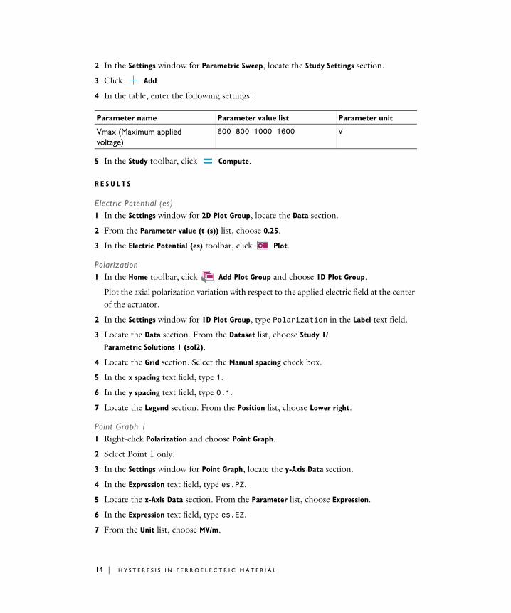
2 In the Settings window for Parametric Sweep, locate the Study Settings section.

3 Click Add.


5 In the Study toolbar, click Compute.

R E S U L T S

Electric Potential (es)1 In the Settings window for 2D Plot Group, locate the Data section.

2 From the Parameter value (t (s)) list, choose 0.25.

3 In the Electric Potential (es) toolbar, click Plot.

Polarization1 In the Home toolbar, click Add Plot Group and choose 1D Plot Group.

Plot the axial polarization variation with respect to the applied electric field at the center of the actuator.

2 In the Settings window for 1D Plot Group, type Polarization in the Label text field.

3 Locate the Data section. From the Dataset list, choose Study 1/

Parametric Solutions 1 (sol2).

4 Locate the Grid section. Select the Manual spacing check box.

5 In the x spacing text field, type 1.

6 In the y spacing text field, type 0.1.

7 Locate the Legend section. From the Position list, choose Lower right.

Point Graph 11 Right-click Polarization and choose Point Graph.

2 Select Point 1 only.

3 In the Settings window for Point Graph, locate the y-Axis Data section.

4 In the Expression text field, type es.PZ.

5 Locate the x-Axis Data section. From the Parameter list, choose Expression.

6 In the Expression text field, type es.EZ.

7 From the Unit list, choose MV/m.

Parameter name Parameter value list Parameter unit

Vmax (Maximum applied voltage)

600 800 1000 1600 V


8 Click to expand the Legends section. Select the Show legends check box.

9 Find the Include subsection. Clear the Point check box.

10 In the Polarization toolbar, click Plot.


Hysteresis in Ferroelectric Material

Documents

Transcript of Hysteresis in Ferroelectric Material