Soil-Pile Dynamic Interaction in the Viscous Damping ... · Soil-Pile Dynamic Interaction in the...

100 The Open Civil Engineering Journal, 2011, 5, 100-108

1874-1495/11 2011 Bentham Open

Open Access

Soil-Pile Dynamic Interaction in the Viscous Damping Layered Soils

Yinhui Wang1, Kuihua Wang

2, Zhixiang Zha

1,* and Renbo Que2

1Department of Civil Engineering and Architecture, Ningbo Institute of Technology, Zhejiang University, Ningbo,

315100, China

2MOE Key Laboratory of Soft Soils and Geoenvironmental Engineering, Zhejiang University, Hangzhou, Zhejiang,

310058, China

Abstract: Modeling surrounding soil as a three-dimensional axisymmetric continuum and considering its wave effect,

soil-pile dynamic longitudinal interaction in viscous layered soils is studied. The pile is assumed to be vertical, elastic and

of uniform section, and the soil is layered and visco-elastic. Longitudinal vibration of pile in viscous damping layered

soils undergoing arbitrary load is theoretically investigated. By taking the Laplace transform, the question can be solved in

frequency domain. Utilizing two potentials combined with impedance transfer functions, analytical solutions for both the

impedance function and mobility at the pile head in frequency domain are yielded. With the convolution theorem and

inverse Fourier transform, a semi-analytical solution of velocity response in time-domain undergoing a half-cycle sine

pulse force is derived. Based on the solutions proposed herein, the effects of variety of soil modulus on mobility curves

and reflection wave curves are emphatically discussed. The results shows that there is a smaller peak between every two

adjacent larger peaks on the mobility curve in layered soil, and larger peak cycle reflects the location where the modulus

of the soil varies abruptly. The conclusions can provide theoretical guidance for non-destruction test of piles.

Keywords: Soil-pile dynamic interaction, Layered soils, Viscous damping, Admittance curves, Mobility curves, Reflection wave curves.

1. INTRODUCTION

Dynamic non-destruction test method based on the pile

vibration theory is widely used to identify pile integrity in

civil engineering. Many soil-pile dynamic interaction models

have been developed to simulate the behavior of longitudinal

vibration of pile. From the view point of different model of

the surrounding soil, they can be put into two categories, that

is, Winkler model [1-7] and continuum model [8-13]. In the

former model, soil is modeled by the distributed Voigt body.

However, the value of parameters in Winkler model, that is,

stiffness of spring and damping of dashpot, can’t correlate

well with the usual soil testing result. What’s more, it is

difficult to consider the wave effect of the surrounding soil.

The first kind of continuum model [8-11] is Plain-Strain

model with assumption that soil consists of independent

infinitesimally thin layers extending to infinity horizontally.

In Plain-Strain model, it is assumed that the gradient of

strain and stress in the vertical direction is zero and the

waves propagate only horizontally. Such assumption does

not match well with reality. The second kind of continuum

model [12, 13] takes the gradient of stress of the surrounding

soil in vertical direction into account and hence can consider

the wave effect of the surrounding soil. Nevertheless, two

import factors, say, the radial displacement and the

*Address correspondence to this author at the Department of Civil

Engineering and Architecture, Ningbo Institute of Technology, Zhejiang

University, Ningbo, 315100, China; Tel: +86-574-88229069;

Fax: +86-574-88229587; E-mail: [email protected]

axisymmetric wave effect of the surrounding soil, are all

neglected in above models. Furthermore, the foundation soil

is layered and this layered nature has a significant impact on

the dynamic response of the pile and hence should be

considered.

Based on above review, the purpose of this paper is to

derive an analytical solution for longitudinal vibration of pile

subjected to harmonic longitudinal excitation in layered soils

by taking the axisymmetric wave effect of the surrounding

soil into account. Utilizing the solution derived herein, the

effects of various soil parameters on the longitudinal

vibration of pile are discussed.

2. FORMULARION

2.1. Pile-Soil System Model

The problem studied herein is the longitudinal vibration

of pile embedded in a layered soil with viscous damping.

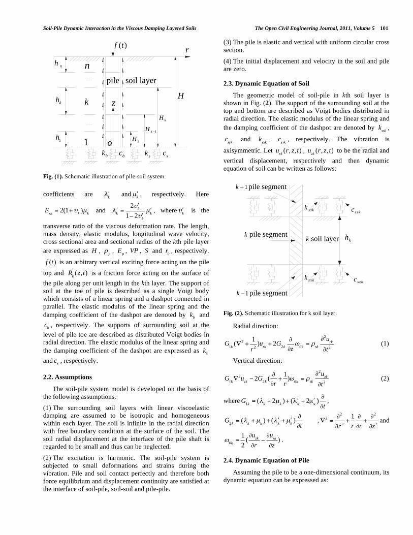
The geometric model is shown in Fig. (1). The soil-pile

system is discretized into a total of n layers numbered by

1, 2, …, n from the pile toe to pile top. The properties of

pile and soil layer are assumed to be homogeneous within

each layer respectively, but may vary from layer to layer. In

the kth soil-pile layer (1 k n) , the mass density, modulus

of compression, thickness, poisson’s ratio, longitudinal wave

velocity, transversal wave velocity of the soil are denoted by

sk,

E

sk,

h

k,

k,

VL

k and

VS

k, respectively. The Lame

constants are k

and μ

k and the corresponding viscosity

Soil-Pile Dynamic Interaction in the Viscous Damping Layered Soils The Open Civil Engineering Journal, 2011, Volume 5 101

coefficients are k

and μ

k, respectively. Here

E

sk= 2(1+

k)μ

k and

k=

2k

1 2k

μk

, where k

is the

transverse ratio of the viscous deformation rate. The length,

mass density, elastic modulus, longitudinal wave velocity,

cross sectional area and sectional radius of the kth pile layer

are expressed as H , p

, E

p, VP , S and

r

0, respectively.

f (t) is an arbitrary vertical exciting force acting on the pile

top and R

k(z, t) is a friction force acting on the surface of

the pile along per unit length in the kth layer. The support of

soil at the toe of pile is described as a single Voigt body

which consists of a linear spring and a dashpot connected in

parallel. The elastic modulus of the linear spring and the

damping coefficient of the dashpot are denoted by b

k and

bc , respectively. The supports of surrounding soil at the

level of pile toe are described as distributed Voigt bodies in

radial direction. The elastic modulus of the linear spring and

the damping coefficient of the dashpot are expressed as s

k

ands

c , respectively.

2.2. Assumptions

The soil-pile system model is developed on the basis of

the following assumptions:

(1) The surrounding soil layers with linear viscoelastic

damping are assumed to be isotropic and homogeneous

within each layer. The soil is infinite in the radial direction

with free boundary condition at the surface of the soil. The

soil radial displacement at the interface of the pile shaft is

regarded to be small and thus can be neglected.

(2) The excitation is harmonic. The soil-pile system is

subjected to small deformations and strains during the

vibration. Pile and soil contact perfectly and therefore both

force equilibrium and displacement continuity are satisfied at

the interface of soil-pile, soil-soil and pile-pile.

(3) The pile is elastic and vertical with uniform circular cross

section.

(4) The initial displacement and velocity in the soil and pile

are zero.

2.3. Dynamic Equation of Soil

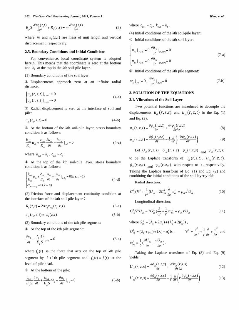
The geometric model of soil-pile in kth soil layer is

shown in Fig. (2). The support of the surrounding soil at the

top and bottom are described as Voigt bodies distributed in

radial direction. The elastic modulus of the linear spring and

the damping coefficient of the dashpot are denoted by k

ssk,

c

ssk and

k

sxk,

c

sxk, respectively. The vibration is

axisymmetric. Let u

rk(r, z, t) ,

u

zk(r, z, t) to be the radial and

vertical displacement, respectively and then dynamic

equation of soil can be written as follows:

Fig. (2). Schematic illustration for k soil layer.

Radial direction:

G

1k( 2

+1

r2

)urk+ 2G

2kz

k=

sk

2u

rk

t2

(1)

Vertical direction:

G

1k

2u

zk2G

2k(

r+

1

r)

k=

sk

2u

zk

t2

(2)

where G

1k= (

k+ 2μ

k)+ ( + 2μ )

t,

G

2k= (

k+μ

k)+ (

k+μ

k)

t ,

2=

2

r2+

1

r r

+2

z2

and

k=

1

2(

uzk

r

urk

z) .

2.4. Dynamic Equation of Pile

Assuming the pile to be a one-dimensional continuum, its

dynamic equation can be expressed as:

Fig. (1). Schematic illustration of pile-soil system.

nh

kh

1h 1

k

n

zH

kH

1H

skbko

( )f t

1kH

bc sc

pile soil layer

r

sskk sskc

kh

sxkksxkc

1k pile segment

k pile segment

1k pile segment

k soil layer

102 The Open Civil Engineering Journal, 2011, Volume 5 Wang et al.

E

pS

2wk(z,t)

z2+ R

k(z, t) = m

2wk(z,t)

t2 (3)

where m and w

k(z, t) are mass of unit length and vertical

displacement, respectively.

2.5. Boundary Conditions and Initial Conditions

For convenience, local coordinate system is adopted

herein. This means that the coordinate is zero at the bottom

and k

h at the top in the kth soil-pile layer.

(1) Boundary conditions of the soil layer:

Displacements approach zero at an infinite radial

distance:

urk

(r, z, t) |r

0

uzk

(r, z, t) |r

0 (4-a)

Radial displacement is zero at the interface of soil and

pile:

u

rk(r

0, z, t) = 0 (4-b)

At the bottom of the kth soil-pile layer, stress boundary

condition is as follows:

ksxk

Esk

uzk+

csxk

Esk

uzk

t

uzk

z|z=0= 0 (4-c)

where k

sx1= k

s,

c

sx1= c

s.

At the top of the kth soil-pile layer, stress boundary

condition is as follows:

kssk

Esk

uzk+

cssk

Esk

uzk

t+

uzk

z|z=h

k

= 0(k n 1)

zk|z=h

k

= 0(k = n)

(4-d)

(2) Friction force and displacement continuity condition at

the interface of the kth soil-pile layer：

R

k(z, t) = 2 r

0 rzk(r

0, z, t) (5-a)

u

zk(r

0, z, t) = w

k(z, t) (5-b)

(3) Boundary conditions of the kth pile segment:

At the top of the kth pile segment:

wk

z

fk(t)

EpS

|z=h

k

= 0 (6-a)

where f

k(t) is the force that acts on the top of kth pile

segment by k +1 th pile segment and f

n(t) = f (t) at the

level of pile head.

At the bottom of the pile:

cbxk

EpS

wk

t+

kbxk

EpS

wk

wk

z|z=0= 0 (6-b)

where c

bx1= c

b,

k

bx1= k

b.

(4) Initial conditions of the kth soil-pile layer:

Initial conditions of the kth soil layer:

urk

|(r ,z ,0)

= 0,u

rk

t|(r ,z ,0)

= 0

uzk

|(r ,z ,0)

= 0,u

zk

t|(r ,z ,0)

= 0

(7-a)

Initial conditions of the kth pile segment:

w

k|( z ,0)

= 0 ,

wk

t|( z ,0)

= 0 (7-b)

3. SOLUTION OF THE EQUATIONS

3.1. Vibrations of the Soil Layer

Two potential functions are introduced to decouple the

displacements u

rk(r, z,t) and

u

zk(r, z,t) in the Eq. (1)

and Eq. (2):

u

rk(r, z, t) = sk

(r,z,t)r

+2

sk(r,z,t)r z

(8)

uzk

(r, z, t) = sk(r,z,t)z

1r r

r sk(r,z,t)r

(9)

Let U

rk(r, z, s)

, U

zk(r, z, s)

, sk(r, z, s)

and sk(r, z, s)

to be the Laplace transform of u

rk(r, z, t) ,

u

zk(r, z,t) ,

sk(r, z, t)

and sk(r, z, t) with respect to t , respectively.

Taking the Laplace transform of Eq. (1) and Eq. (2) and

combining the initial conditions of the soil layer yield:

Radial direction:

G

1k

L ( 2+

1

r2

)Urk+ 2G

2k

L

zk

L=

sks

2U

rk (10)

Longitudinal direction:

G

1k

L 2U

zk2G

2k

L (r+

1

r)

k

L=

sks

2U

zk (11)

where G

1k

L = (k+ 2μ

k)+ ( + 2μ )s ,

G

2k

L = (k+μ

k)+ (

k+μ

k)s ,

2=

2

r2+

1

r r

+2

z2

and

k

L=

1

2(

Uzk

r

Urk

z) .

Taking the Laplace transform of Eq. (8) and Eq. (9)

yields:

U

rk(r, z, s) = sk

(r,z,s)r

+2

sk(r,z,s)r z

(12)

Uzk

(r, z, s) = sk(r,z,s)z

1r r

r sk(r,z,s)r

(13)


Substituting Eq. (12) and Eq. (13) into Eq. (10) and Eq.

(11) yields:

G

1k

L

r

2

sk+ μ

k+μ

ks( )

2

r z

2

sk=

sks

2 ( sk

r+

2sk

r z) (14)

G1k

L

z

2

skμ

k+μ

ks( )

2

r2+ 1

r r( ) 2

sk

=sk

s2 sk

z

2

r2+ 1

r r( ) sk

(15)

And thus Eq. (14) and Eq. (15) can be decoupled as

follows:

2

sk

s2

lk

2 sk= 0 (16)

2

sk

s2

vsk

2 sk= 0 (17)

where

lk=

G1k

L

sk

,

sk=

μk+μ

ks

sk

,

k=

2(1k)

1 2k

;

VLk= k

+ 2μk

sk

and

VSk=

μk

sk

are longitudinal wave and

shear wave velocity of the kth soil layer, respectively.

Solving Eq. (16) and Eq. (17) with method of separation

of variables first and then combining Eq. (12) and Eq. (13),

we can obtain the solutions of U

rk(r, z, s) and

U

zk(r, z, s) as

follows:

Urk

(r, z, s) = [A1k

cos(kz)+ B

1ksin(

kz)]

[C1k

I1(

kr) D

1kK

1(

kr)]

k

[A2k

sin(kz) B

2kcos(

kz)]

[C2k

I1(s

kr) D

2kK

1(s

kr)]

ks

k

(18)

Uzk

(r, z, s) = [B1k

cos(kz) A

1ksin(

kz)]

[C1k

I0(

kr)+ D

1kK

0(

kr)]

k

[A2k

cos(kz)+ B

2ksin(

kz)]

[C2k

I0(s

kr)+ D

2kK

0(s

kr)]s

k

2

(19)

where I

0() and K0 () are modified Bessel functions of order

zero of the first and second kind, respectively; I

1() and

K

1() are modified Bessel functions of order first of the first

and second kind, respectively. A

1k, B

1k, C

1k, D

1k, A

2k, B

2k,

C

2k,

D

2k and

k are constants to be determined by the

boundary conditions. k

and s

k satisfy the following rela-

tionship:

k

2

k

2=- s2

lk

2 (20)

k

2s

k

2= s2

sk

2 (21)

For convenience, repeat Eq. (4-a) here:

urk

(r, z, t) |r

0

uzk

(r, z, t) |r

0 (22)

Take the Laplace transform of Eq. (22):

Urk

(r, z, s) |r

0

Uzk

(r, z, s) |r

0 (4-a’)

Similarly, taking the Laplace transform of Eq.(4-b) to (4-

d) as follows:

U

rk(r

0, z, s) = 0 (4-b’)

(k

sxk

Esk

+c

sxk

Esk

s)Uzk

(r, z, s)U

zk(r, z, s)

z|z=0= 0 (4-c’)

(k

ssk

Esk

+c

ssk

Esk

s)Uzk

(r, z, s)+U

zk(r, z, s)

z|z=h

k

= 0

[(n+ 2μ

n)+ (

n+ 2μ

n)s]

Uzn

z+ (

n+

ns)

(rUrn

)

r r|z=h

n

= 0

(4-d’)

Substituting Eq. (18) and Eq. (19) into Eq. (4-a’) to (4-d’)

and solving them simultaneously yields U

rk(r, z, s) and

U

zk(r, z, s) :

Urk

(r, z, s) = akm

Mkm

sin(km

zkm

)km

[K1(

kmr)

K1(

kmr

0k)

K1(s

kmr

0k)

K1(s

kmr)]

m=1

Uzk

(r, z, s) = akm

Mkm

cos(km

zkm

)[ kmK

1(

kmr

0k)

kmK

1(s

kmr

0k)

skm

K0(s

kmr)

kmK

0(

kmr)]

m=1

(23)

where a

km is a constants to be determined.

km,

km,

s

km,

km and

M

km can be obtained from the following equations:

tan(km

hk) =

(KXk+ KS

k)

km

km

2KX

kKS

k

(24)

km

2

km

2= - s2

lk

2 (25)

km

2s

km

2= s2

sk

2 (26)

tan(km

) =KX

k

km

(27)

Mkm= 1+ ( km

KXk

)2 (28)

where

KSk=

kssk+ c

ssks

Esk

(k < n)

KSk= 0(k = n)

KXk=

ksxk+ c

sxks

Esk

(29)


3.2. Solution for Longitudinal Vibrations of the Pile

Denote W

k(z, s) as the Laplace transform with respect to

time of w

k(z, t) and take the Laplace transform of Eq. (3).

After using the initial condition (7-b), we can get:

d2Wk(z,s)

dz2+ p2W

k(z, s) =

Rk(z, s)

EpS

(30)

where

p2=

s2

VP2

.

Rewrite boundary condition (5-a) as :

Rk(z, s) = 2 r

0(μ

k+μ

ks)

akm

Mkm

cos(km

zkm

)(km

2s

km

2 ) km

km

K1(

kmr

0)

m=1

(31)

Then solving Eq. (30) for W

k and using boundary

condition Eq.(31) gives:

Wk= Asin( pz)+ B cos( pz)+ C

kmcos(

kmz

km)

m=1

(32)

where

Ckm= C

kma

km

Ckm=

2 r0(μ

k+μ

ks)M

km(s

km

2

km

2 )km

K1(

kmr

0)

EpS( p2

km

2 )km

(33)

Taking the Laplace transform of Eq. (5-b) gives

U

zk(r

0, z, s) =W

k(z, s) , which can be further rewritten as

follows:

akm

Dkm

cos(km

zkm

)m=1

= Ckm

cos(km

zkm

)m=1

+ Asin( pz)+ B cos( pz)

(34)

where

Dkm= M

km[

kmK

0(

kmr

0) km

K1(

kmr

0)

kmK

1(s

kmr

0)

skm

K0(s

kmr

0)] (35)

It can be proved that cos(

kmz

km) form an orthogonal

set over the interval [0, h

k] as follow:

cos(km

zkm

)0

hk

cos(kn

zkn

)dz 0(m = n)

cos(km

zkm

)0

hk

cos(kn

zkn

)dz = 0(m n)

(36)

Multiplying both sides of Eq. (34) by

2

hk

cos(km

zkm

) and

then integrating over the interval [0, h

k] , we can get

W

k :

Wk=

Fk1m

Ckm

cos(km

zkm

)

(Dkm

Ckm

)Fk 3mm=1

+ sin( pz) A

+F

k 2mC

kmcos(

kmz

km)

(Dkm

Ckm

)Fk 3mm=1

+ cos( pz) B

(37)

where

Fk1m

=2

hk

sin( pz) cos(km

zkm

)dz0

hk

Fk 2m

=2

hk

cos( pz) cos(km

zkm

)dz0

hk

Fk 3m

=2

hk

cos(km

zkm

) cos(km

zkm

)dz0

hk

. (38)

Denoting F

k(s) as the Laplace transform of

f

k(t) with

respect to t and taking the Laplace transform of the

boundary conditions Eq. (6-a) and Eq. (6-b) yields:

dWk

dz

Fk(s)

EpS

|z=h

k

= 0 (6-a’)

E

pS

dWk

dz= (k

bxk+ c

bxks)W

k|z=0

(6-b’)

Substituting Eq. (37) into Eq. (6-a’) to (6-b’) and solving

for A and B , we can obtain the impedance function at the

kth pile segment head:

(39)

where

L1k=

Fk1m

Ckm km

(Dkm

Ckm

)Fk 3m

sin(km

hk km

)m=1

+ p cos( phk) ,

N1k=

Fk 2m

Ckm km

(Dkm

Ckm

)Fk 3m

sin(km

hk km

)m=1

p sin( phk) ,

L2k=

Ckm

Fk1m

[Z

k 1

EpS

cos(km

)km

sin(km

)]

(Dkm

Ckm

)Fk 3mm=1

p ,

N2k=

Ckm

Fk 2m

[Z

k 1

EpS

cos(km

)km

sin(km

)]

(Dkm

Ckm

)Fk 3mm=1

+Z

k 1

EpS

.

And then the velocity admittance function at the kth pile

segment can be obtained as follows:

Gvk

(s) =s

Zk(s)

(40)

Set i = 1 , and

Tk=

hk

VPto be the imaginary unit,

the circular frequency and the propagating time in the kth

pile segment, respectively. For convenience, some

dimensionless parameters are introduced as follows:

r0k=

r0

hk

;

k= sk

p

; v

spk=

VSk

VP;

k=

2vspk

2

k

r0k

2

; p

k= T

k;

Dμ=

μk

μkT

k

;

D = k

kT

k

;

Rxk=

ksxk

hk

Esk

;

Ixk=

csxk

hk

Esk

Tk

;

Zk(s) =

Fk(s)

Wk(h

k, s)

=E

pS

hk

(L1k

N2k

L2k

N1k

)hk

{[C

kmcos(

kmz

km)

(Dkm

Ckm

)Fk 3m

(N2k

Fk1m

m=1

L2k

Fk 2m

)+ [N2k

sin( pz) L2k

cos( pz)]}


KX

k= (R

xk+ iI

xkp

k) ;

Rsk=

kssk

hk

Esk

;

Isk=

cssk

hk

Esk

Tk

; k

=kh

k;

KS

k= (R

sk+ iI

skp

k) ;

ask=

hk

VSk

;

Mkm= 1+ ( km

KXk

)2 ;

sk=

k

2

(a

sk

1+ iDμ

pk

)2;

k=

k

2

(a

sk

2 + i[( 2 2)D + 2Dμ]p

k

)2;

Rb=

kbh

1

EpS ;

Ib=

cbh

1

EpST

1

; Z

0= R

b+ iI

bp

1 ;

Ckm=

k

r0k

(1+ iDμ

pk)M

km(s

km

2

km

2

) km

km

K1(

kmr0k

)

pk

2

km

2;

Dkm= M

km[ km

K1(

kmr0k

)

kmK

1(s

kmr0k

)s

kmK

0(s

kmr0k

)km

K0(

kmr0k

)] ;

Zk 1=

hk

EpS

Zk 1

;

Fk1m

=cos(

km) cos[( p

k+

km)

km]

pk+

km

+cos(

km) cos[( p

k km)+

km]

pk km

;

Fk 2m

=sin[( p

k+

km)

km]+ sin(

km)

pk+

km

+sin[( p

k km)+

km] sin(

km)

pk km

;

Fk 3m

=sin[2(

km km)]+ sin(2

km)

2km

+1 ;

L1k=

Fk1m

Ckm km

(Dkm

Ckm

)Fk 3m

sin(km km

)m=1

+ pkcos( p

k) ;

L2k=

Ckm

Fk1m

[Zk 1

cos(km

)km

sin(km

)]

(Dkm

Ckm

)Fk 3mm=1

pk

;

N1k=

Fk 2m

Ckm km

(Dkm

Ckm

)Fk 3m

sin(km km

)m=1

pk

sin( pk) ;

N2k=

Ckm

Fk 2m

[Zk 1

cos(km

)km

sin(km

)]

(Dkm

Ckm

)Fk 3m

m=1

+ Zk 1

;

DNk= N

2k[

Fk1m

Ckm

cos(km km

)

(Dkm

Ckm

)Fk 3mm=1

+ sin( pk)]

L2k

[F

k 2mC

kmcos(

km km)

(Dkm

Ckm

)Fk 3mm=1

+ cos( pk)]

.

where k

and km

can be determined utilizing the following

equations:

tan(k) =

[KXk+ KS

k]

k

[k

2

KXkKS

k]

(41)

tan(km

) =KX

k

km

(42)

where equation (41) is a complex transcendental equation

and can be solved by numerical method.

Substituting s i= into Eq. (39) to (40), the

displacement impedance function and velocity admittance at

the head of kth pile segment can be expressed as follows:

Kdk=

EpS

hk

Kdk

(41)

Hvk

( ) =1

pS VP

Hvlk

(42)

where K

dk and

H

vlk are dimensionless displacement

impedance function and velocity admittance function,

respectively:

Kdk= Z

k=

(L1k

N2k

L2k

N1k

)

DNk

(43)

Hvlk=

1

Zk

i pk

(44)

Set k n= in Eq. (41) and Eq. (42) and then the

displacement impedance function and velocity admittance at

the pile head can be obtained.

When the excitation acting on the pile head is a half-sine

pulse such as f (t) =Q

maxsin(

Tt) ,

t (0,T ) , where T

denotes the impulse width, then the semi-analytical velocity

response of the pile head can be expressed as:

gn(t) = Q

maxIFT (H

vn

T2

T2 2

(1+ ei T )) =

Qmax

pS VP

gn(t) (45)

gn(t) =

1

2H

v ln

T

2 T 22

(1+ e i T )ei t d (46)

where

Tc=

hk

VPi=1

n

denotes the propagation time of elastic

longitudinal wave propagating from the pile head to pile tip.

t =t

Tc

,

T =T

Tc

and = T

c denote the dimensionless

time, dimensionless impulse width and dimensionless

circular frequency, respectively.

4. PARAMETRIC STUDY AND DISCUSSION

In the following, the effects of variety of soil modulus on

the velocity admittance curves and reflection wave curves


are discussed, which are the theoretical basis of mechanical

impedance analysis method and reflection wave method. For

convenience, the subscripts marking the soil layer are

eliminated if the parameter values are same in each layer in

the following figures. Number sequence of the soil layer is

shown in Fig. (1). Parameters using in the analysis are shown

as follows:

V

ij=VS

i/ VS

j VP = 3500、 r

0= 0.5、

p= 2500、

c

b= 5 10

5、 k

b=10

9、 = 0.4、 = 0.4、 μ = 5 10

3、

= 0.7、

ksxk

Esk

=1、 c

sxk=104、

kssk

Esk

(k < n) =1、

c

sxk(k < n) =104、 T =1.5ms .

The case of two soil layers: Influence of modulus of

upper soil layer on the velocity admittance curve and

reflection wave curve at the pile top

Fig. (3.a) shows that the variation of modulus of the

upper soil layer has significant effect on the velocity

admittance curve. Compared with the case that the soil is

homogeneous, the velocity admittance curve of the pile top

has a phenomenon that there is a smaller peak between every

two adjacent larger peaks. When the upper soil layer is

stiffer than the lower soil layer, it can be seen that the

amplitude of the velocity admittance increase at first as the

frequency increases, but then decrease as the frequency

further increases after the amplitude is beyond the

maximum. When the upper soil layer is softer than the lower

soil layer, it can be seen that the amplitude of the velocity

admittance decrease as the frequency increases and the

amplitude increase as the frequency further increases after

the amplitude is beyond the minimum. For two cases, the

length between every two adjacent larger peaks (large peak

cycle) is almost equal, which reflects the location where the

soil impedance varies abruptly with the relationship

h

2VP / d

max=10.18m . The length between one larger

peak and its corresponding adjacent smaller peak (smaller

peak cycle) reflects the pile length with the relationship

H VP / d =19.64m . Fig. (3.b) shows that wave curve

at the division surface concaves and is out of phase with the

input pulse when the upper soil layer is stiffer than the lower

soil layer. The wave curve at the division surface convexes

and is in phase with the input pulse when the upper soil layer

is softer than the lower soil layer.

Fig. (4.a) and Fig. (4.b) show that the amplitude of the

velocity admittance decreases as the modulus of the upper

soil layer increases and oscillation is weak. The dynamic

stiffness at the low frequency range increases and the

amplitude of the input impulse and the reflection amplitude

at the pile tip decreases. The amplitude of the reflected wave

amplitude at the division surface increases. It is due to more

energy dissipation in the shallow layer as the modulus of the

upper soil layer increases.

The case of three soil layers: Influence of modulus of

surrounding soil on the velocity admittance curve and

reflection wave curve at the pile top

a

b

Fig. (3). Influence of Variations of modulus of upper soil layer on velocity admittance curve and reflection wave curve.

a

b

Fig. (4). Influence of varying degree of modulus of upper soil layer on velocity admittance curve and reflection wave curve.

0 500 1000 1500 2000 2500 3000 3500 4000 45000.0

0.2

0.4

0.6

0.8

1.0

1.2

1.4

1.6

5601080

ddmax

VS1/VP=0.04

h2=h

1=10m

H' v

V21=0.5V21=1V21=2

0.000 0.004 0.008 0.012 0.016 0.020 0.024 0.028-0.4

-0.2

0.0

0.2

0.4

0.6

0.8

1.0

VS1/VP=0.04

h2=h

1=10m

g't

V21=0.5V21=1V21=2

0 500 1000 1500 2000 2500 3000 3500 4000 45000.0

0.2

0.4

0.6

0.8

1.0

1.2

VS1/VP=0.04

h2=h

1=10m

H' v

V21=2V21=1.5V21=1

0.000 0.004 0.008 0.012 0.016 0.020 0.024 0.028-0.4

-0.2

0.0

0.2

0.4

0.6

0.8

1.0

VS1/VP=0.04

h2=h

1=10m

g'

t

V21=2V21=1.5V21=1


Fig. (5.a) and Fig. (5.b) show that the velocity admittance

curve is similar to the case of two soil layers when there is

stiffer or softer interlayer in the surrounding soil. Large peak

cycle reflects the location of the interlayer with the

relationship 3 max

/ 6.5h VP d m= . At the first peak, the

amplitude of the case with stiffer interlayer is larger than that

of the case with homogeneous soil and the amplitude of the

case with softer interlayer is smaller than that of the case

with homogeneous soil. Consequently, the properties of the

upper soil layer have significant effect on the amplitude of

the first peak. The wave curve at the division surface is out

of phase with the input pulse for stiffer interlayer case and in

phase with the input pulse for softer interlayer case. The

amplitude of the reflection wave at the pile tip decrease as

the modulus of the stiffer or softer interlayer increases.

a

b

Fig. (5). Influence of hard or soft interlayer on velocity admittance curve and reflection wave curve.

Fig. (6.a) and Fig. (6.b) show that the occurring time of

the reflected waves of the interlayer is retarded as the buried

depth of the softer layer becomes deeper. The large peak

cycle of the velocity admittance curve reflects the buried

depth of the interlayer with the relationship

3 max1 max 2 max 3/ / / 6.39 /8.46 /10.18h VP d d d m m m= .

Fig. (7.a) and Fig. (7.b) show that the amplitude of the

velocity admittance increases but the reflection amplitude of

the interlayer tends to be weaker as the thickness of the

softer interlayer increases. The reflection amplitude at the

pile tip increase. It is due to less energy dissipation in the

interlayer as its thickness increases.

a

b

Fig. (6). Influence of location of soft interlayer on velocity admittance curve and reflection wave curve.

a

b

Fig. (7). Influence of length of soft interlayer on velocity admittance curve and reflection wave curve.

0 500 1000 1500 2000 2500 3000 3500 4000 45000.0

0.2

0.4

0.6

0.8

1.0

1.2

1.4

1.6

1680

dmax2

1680

dmax1

V31=1

h3=6mh

2=2mh

1=12m

VS1/VP=0.04

H' v

V21=0.5V21=1V21=2

0.000 0.004 0.008 0.012 0.016 0.020 0.024 0.028-0.4

-0.2

0.0

0.2

0.4

0.6

0.8

1.0V31=1

VS1/VP=0.04

h1=12m h

2=2m h

3=6m

g'

t

V21=0.5V21=1V21=2

0 500 1000 1500 2000 2500 3000 3500 4000 45000.0

0.2

0.4

0.6

0.8

1.0

1.2

1.4

1.6

dmax2

=1300 dmax3

=1080

dmax1

=1720

VS1/VP=0.04

V21=0.5V31=1H=20mh

2=2m

H' v

h3=6m

h3=8m

h3=10m

0.000 0.004 0.008 0.012 0.016 0.020 0.024 0.028-0.2

0.0

0.2

0.4

0.6

0.8

1.0

VS1/VP=0.04

V21=0.5V31=1H=20mh

2=2m

g'

t

h3=6m

h3=8m

h3=10m

0 500 1000 1500 2000 2500 3000 3500 4000 45000.0

0.2

0.4

0.6

0.8

1.0

1.2

1.4

VS1/VP=0.04

V21=0.5V31=1H=20mh

3=6m

H' v

h2=2m

h2=4m

h2=6m

0.000 0.004 0.008 0.012 0.016 0.020 0.024 0.028-0.2

0.0

0.2

0.4

0.6

0.8

1.0

VS1/VP=0.04

V21=0.5V31=1H=20mh

3=6m

g'

t

h2=2m

h2=4m

h2=6m


5. CONCLUSIONS

(1) Modeling surrounding soil as a three-dimensional

axisymmetric continuum and considering its wave effect,

soil-pile dynamic longitudinal interaction in viscous layered

soils is studied. The analytical solution of mobility in the

frequency domain and semi-analytical solution of velocity

response in the time domain undergoing a half-cycle sine

pulse force have been derived. Based on the solutions herein,

the effect of stiffer or softer interlayer on the mobility curves

and reflection wave curves of integrated pile is studied

(2) Compared with the case of homogeneous soil, there is a

smaller peak between every two adjacent larger peaks on the

mobility curve in layered soil. The difference between two

adjacent larger peaks can be used to locate where abrupt

variety of soil modulus happens. At the division surface, the

reflection wave curve is out of phase with the input pulse if

soil modulus increases and in phase with the input pulse if

soil modulus decreases.

REFERENCES

[1] K. H. Van, P. Middendorp, and B. P Van, “An analysis of

dissipative wave propagation in a pile”, Intl seminar on the application of Stress-Wave Theory onpiles/Stockholm, 1980.

[2] D. W. Chang and S. H. Yeh, “Time-domain wave equation analyses of single piles utilizing tansformed radiation damping”,

Soils and Foundations, JGS, vol. 39, no.2, pp. 31- 44, 1999. [3] W. Teng, W. Kuihua, and X. Kanghe, “Study on vibration

properties of piles in layered soils”, China Civil Engineering Journal, vol. 35, no. 1, pp. 83-87, 2001. (in Chinese).

[4] L. Dongjia, “Dynamic axial response of multi-defective piles in

nonhomogeneous soil”, Chinese Journal of Geotechnical Engineering, vol. 22, no. 4, pp. 391-395, 2002. (in Chinese).

[5] W. Kuihua, “Vibration of inhomogeneous viscous-elastic pile embedded in layered soils with general Voigt model”, Journal of

Zhejiang University (Engineering Science), vol. 36, no. 5, pp. 565-571, 595, 2002. (in Chinese).

[6] W. Kuihua and Y. Hongwei, “Vibration of inhomogeneous pile embedded in layered soils with general Voigt model”, Acta Mechanica

Solida Sinica, vol. 24, no. 3, pp. 293-303, 2003. (in Chinese). [7] F. Shijin, C. Yunmin, and L. Mingzhen, “Analysis and application

in engineering on vertical vibration of viscoelasticity piles in layered soil”, China Journal of Highway and Transport, vol. 17,

no. 2, pp. 59-63, 2004. (in Chinese). [8] T. Nogami and M. Novak, “Soil-pile interaction in vertical

vibration”, Earthquake Engineering and Structural Dynamics, vol. 4, pp. 277-293, 1976.

[9] M. Novak and F. Aboul-Ella, “Impedance functions of piles in layered media”, Journal of the Engineering Mechanics Division,

ASCE, vol. 104, pp. 643-661, 1978. [10] M. Novak, T. Nogami, and F. Aboul-Ella, “Dynamic soil reactions

for plane strain case”, Journal of the Engineering Mechanics Division, ASCE, vol.104 (EM4), pp. 953-959, 1978.

[11] G. Militano and R. K. N. D. Rajapakse, “Dynamic response of a pile in a multi-layered soil to transient torsional and axial loading”,

Geotechnique, vol. 49, no. 1, pp. 91-109, 1999. [12] H. Changbin, W. Kuihua, and X. Kanghe, “Time domain analysis

of vertical dynamic response of a pile considering the effect of pile-soil interaction”, Chinese Journal of Computational

Mechanics, vol. 21, no. 4, pp. 392-399, 2004. (in Chinese). [13] H. Changbin, W. Kuihua, and X. Kanghe, “Time Domain Axial

Response of Dynamically Loaded Pile in Viscous Damping Soil Layer”, Journal of Vibration Engineering, vol. 17, no.1, pp. 72-77,

2004. (in Chinese).

Received: September 01, 2010 Revised: November 21, 2010 Accepted: January 03, 2011

© Wang et al.; Licensee Bentham Open.

This is an open access article licensed under the terms of the Creative Commons Attribution Non-Commercial License

(http://creativecommons.org/licenses/ by-nc/3.0/) which permits unrestricted, non-commercial use, distribution and reproduction in any medium, provided the work is properly cited.

Soil-Pile Dynamic Interaction in the Viscous Damping ... · Soil-Pile Dynamic Interaction in the...

Documents

Transcript of Soil-Pile Dynamic Interaction in the Viscous Damping ... · Soil-Pile Dynamic Interaction in the...