Specification Techniques and

Formal Specifications

System models are abstract descriptions of systems whose requirements are being analysed

Objectives To explain why specification modelling techniques

help discover problems in system requirements To describe

– Behavioural modelling (FSM, Petri-nets), – Data modelling and – Object modelling (Unified Modeling Language,

UML)

Formal Specification - Techniques for the unambiguous specification of software

Objectives: To explain why formal specification techniques

help discover problems in system requirements To describe the use of

– algebraic techniques (for interface specification) and

– model-based techniques(for behavioural specification)

System modelling

System modelling helps the analyst to understand the functionality of the system and models are used to communicate with customers

Different models present the system from different perspectives– External perspective showing the system’s context or

environment– Behavioural perspective showing the behaviour of the

system– Structural perspective showing the system or data

architecture

System models weaknesses

They do not model non-functional system requirements

They do not usually include information about whether a method is appropriate for a given problem

They may produce too much documentation The system models are sometimes too detailed

and difficult for users to understand

Model types

Data processing model showing how the data is processed at different stages

Composition model showing how entities are composed of other entities

Architectural model showing principal sub-systems

Classification model showing how entities have common characteristics

Stimulus/response model showing the system’s reaction to events

1. Context models

Context models are used to illustrate the boundaries of a system

Social and organisational concerns may affect the decision on where to position system boundaries

Architectural models show the a system and its relationship with other systems

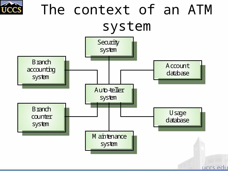
The context of an ATM system

Auto-tellersystem

Securitysystem

Maintenancesystem

Accountdatabase

Usagedatabase

Branchaccounting

system

Branchcountersystem

Process models

Process models show the overall process and the processes that are supported by the system

Data flow models may be used to show the processes and the flow of information from one process to another

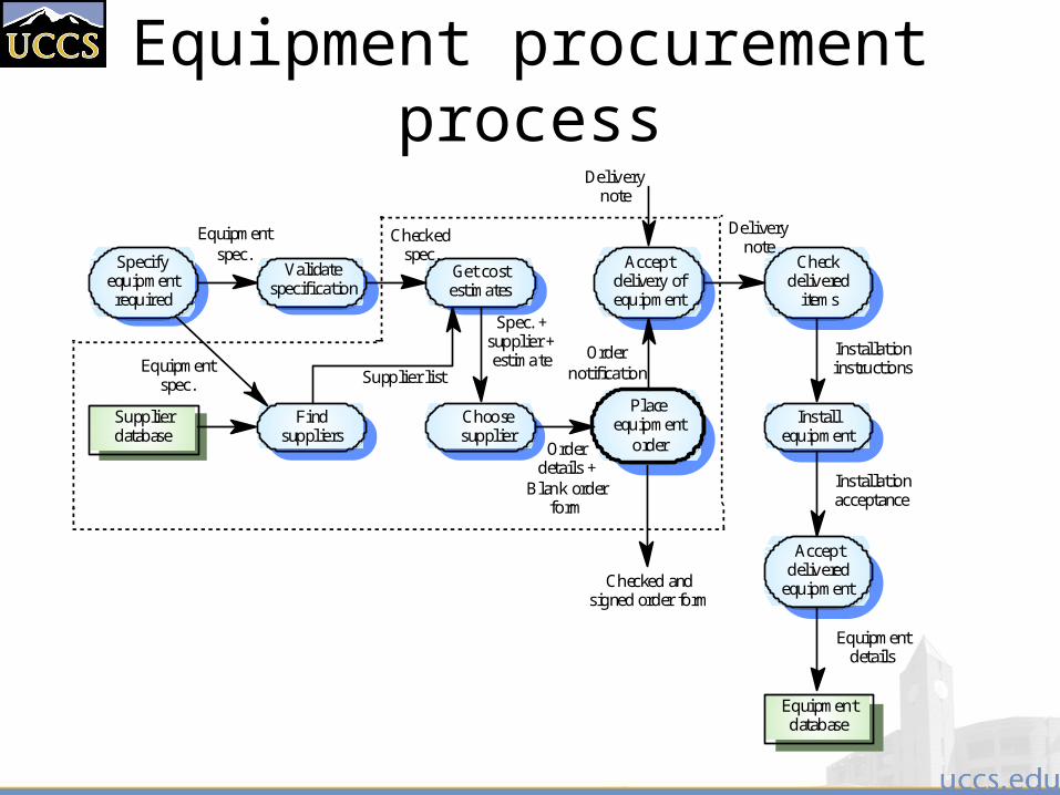
Equipment procurement process

Get costestimates

Acceptdelivery ofequipment

Checkdelivered

items

Validatespecification

Specifyequipmentrequired

Choosesupplier

Placeequipment

order

Installequipment

Findsuppliers

Supplierdatabase

Acceptdelivered

equipment

Equipmentdatabase

Equipmentspec.

Checkedspec.

Deliverynote

Deliverynote

Ordernotification

Installationinstructions

Installationacceptance

Equipmentdetails

Checked andsigned order form

Orderdetails +

Blank orderform

Spec. +supplier +estimate

Supplier listEquipment

spec.

Semantic data models

Used to describe the logical structure of data processed by the system

Entity-relation-attribute model sets out the entities in the system, the relationships between these entities and the entity attributes

Widely used in database design. Can readily be implemented using relational databases

No specific notation provided in the UML but objects and associations can be used

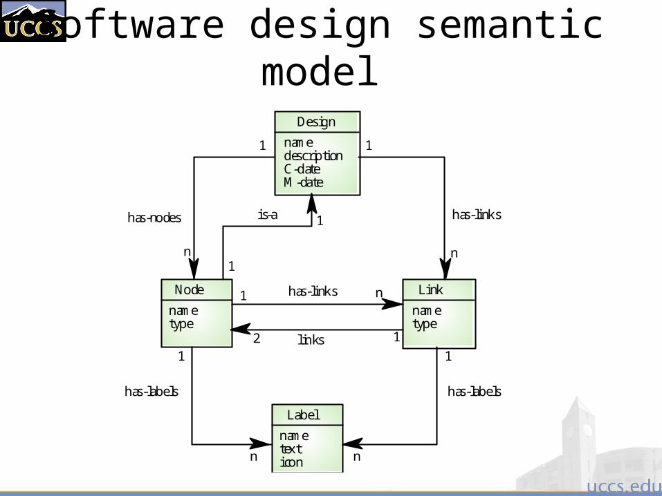
Software design semantic modelDesign

namedescriptionC-dateM-date

Link

nametype

Node

nametype

links

has-links

12

1 n

Label

nametexticon

has-labelshas-labels

1

n

1

n

has-linkshas-nodes is-a

1

n

1

n1

1

Data dictionary entries

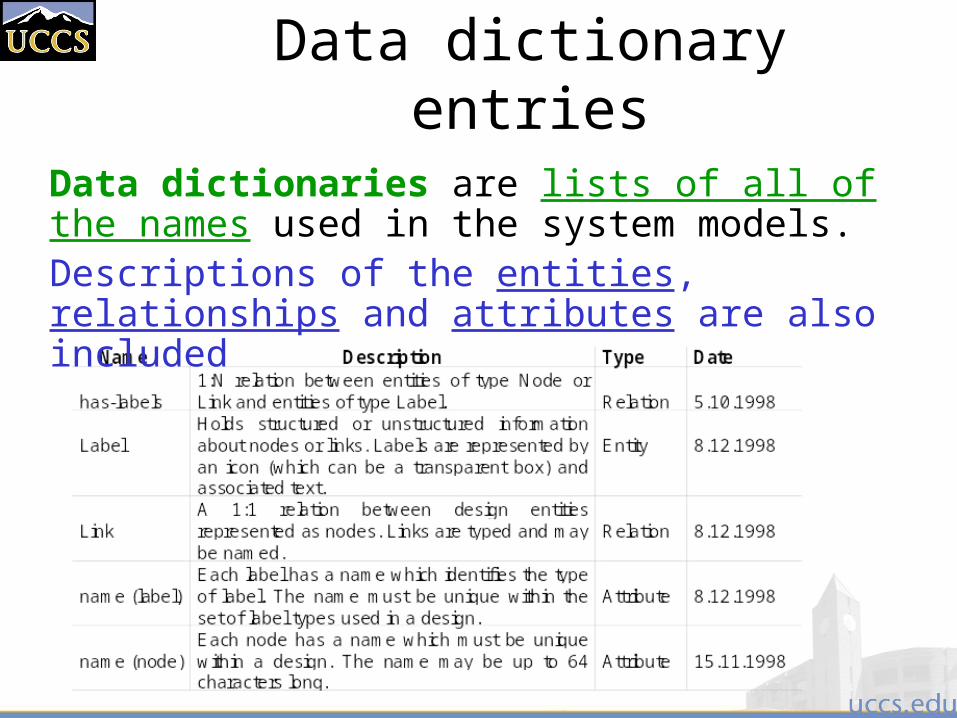
Data dictionaries are lists of all of the names used in the system models. Descriptions of the entities, relationships and attributes are also included

Object models

Object models describe the system in terms of object classes

An object class is an abstraction over a set of objects with common attributes and the services (operations) provided by each object

Various object models may be produced– Inheritance models– Aggregation models– Interaction models

Object models

Natural ways of reflecting the real-world entities manipulated by the system

More abstract entities are more difficult to model using this approach

Object class identification is recognised as a difficult process requiring a deep understanding of the application domain

Object classes reflecting domain entities are reusable across systems

The Unified Modeling Language Devised by the developers of widely used object-

oriented analysis and design methods Has become an effective standard for object-oriented

modelling Notation

– Object classes are rectangles with the name at the top, attributes in the middle section and operations in the bottom section

– Relationships between object classes (known as associations) are shown as lines linking objects

– Inheritance is referred to as generalisation and is shown ‘upwards’ rather than ‘downwards’ in a hierarchy

Behavioural models

Behavioural models are used to describe the overall behaviour of a system

Two types of behavioural model– Data processing models that show how data is

processed as it moves through the system– State machine models that show the systems

response to events Both of these models are required for a

description of the system’s behaviour

Data Flow Diagrams

Data flow diagrams are used to model the system’s data processing

These show the processing steps as data flows through a system

IMPORTANT part of many analysis methods

Simple and intuitive notation that customers can understand

Show end-to-end processing of data

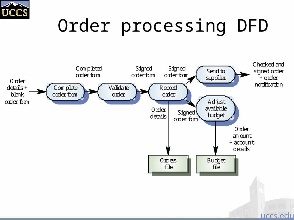
Order processing DFD

Completeorder form

Orderdetails +

blankorder form

Valida teorder

Recordorder

Send tosupplier

Adjustavailablebudget

Budgetfile

Ordersfile

Completedorder form

Signedorder form

Signedorder form

Checked andsigned order

+ ordernotification

Orderamount

+ accountdetails

Signedorder form

Orderdetails

Data flow diagrams

DFDs model the system from a functional perspective

Tracking and documenting how the data associated with a process is helpful to develop an overall understanding of the system

Data flow diagrams may also be used in showing the data exchange between a system and other systems in its environment

State machine models

State Machine models the behaviour of the system in response to external and internal events

They show the system’s responses to stimuli so are often used for modelling real-time systems

State machine models show system states as nodes and events as arcs between these nodes. When an event occurs, the system moves from one state to another

Statecharts are an integral part of the UML

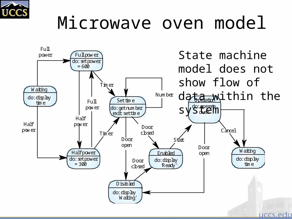
Microwave oven model

Full power

Enabled

do: operateoven

Fullpower

Halfpower

Halfpower

Fullpower

Number

TimerDooropen

Doorclosed

Doorclosed

Dooropen

Start

do: set power = 600

Half powerdo: set power = 300

Set time

do: get numberexit: set time

Disabled

Operation

Timer

Cancel

Waiting

do: display time

Waiting

do: display time

do: display 'Ready'

do: display 'Waiting'

State machine model does not show flow of data within the system

Microwave oven stimuli

Finite state machines

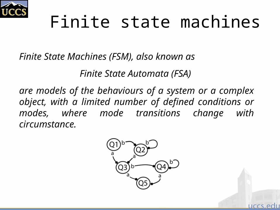
Finite State Machines (FSM), also known as

Finite State Automata (FSA)

are models of the behaviours of a system or a complex object, with a limited number of defined conditions or modes, where mode transitions change with circumstance.

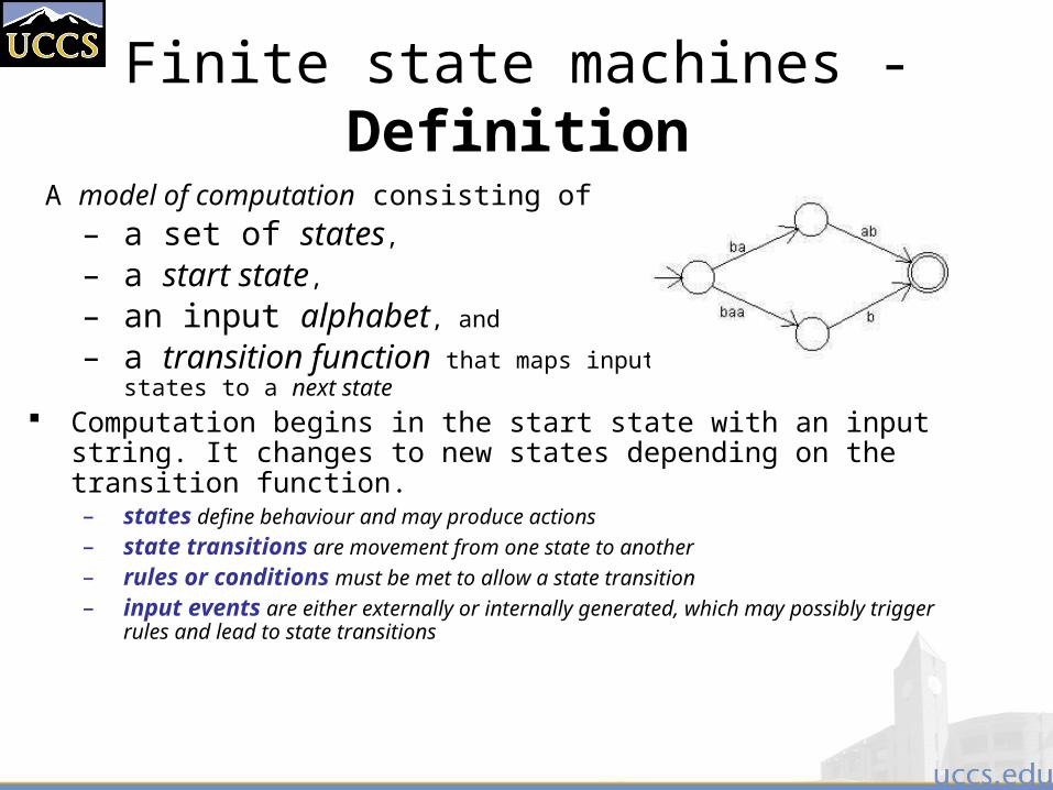
Finite state machines - Definition

A model of computation consisting of– a set of states,

– a start state,

– an input alphabet, and

– a transition function that maps input symbols and current states to a next state

Computation begins in the start state with an input string. It changes to new states depending on the transition function. – states define behaviour and may produce actions – state transitions are movement from one state to another – rules or conditions must be met to allow a state transition– input events are either externally or internally generated, which

may possibly trigger rules and lead to state transitions

Variants of FSMs

There are many variants, for instance,

– machines having actions (outputs) associated with transitions (Mealy machine) or states (Moore machine),

– multiple start states, – transitions conditioned on no input symbol (a

null) or more than one transition for a given symbol and state (nondeterministic finite state machine),

– one or more states designated as accepting states (recognizer), etc.

Finite State Machines with Output (Mealy and Moore Machines)

Finite automata are like computers in that they receive input and process the input by changing states. The only output that we have seen finite automata produce so far is a yes/no at the end of processing.

We will now look at two models of finite automata that produce more output than a yes/no.

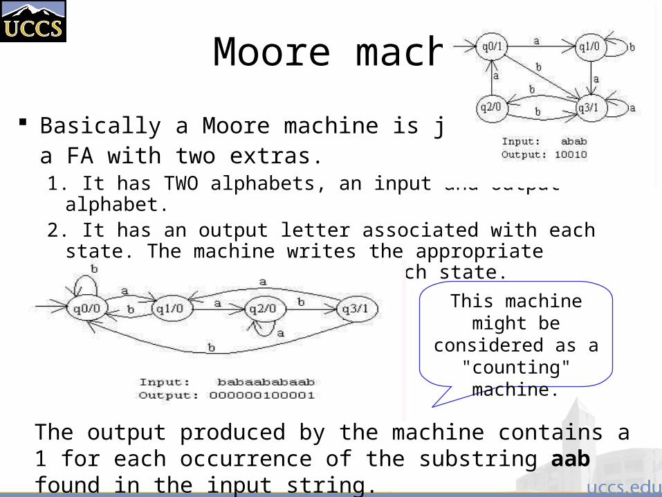
Moore machine

Basically a Moore machine is just a FA with two extras. 1. It has TWO alphabets, an input and output alphabet. 2. It has an output letter associated with each state. The

machine writes the appropriate output letter as it enters each state.

The output produced by the machine contains a 1 for each occurrence of the substring aab found in the input string.

This machine might be considered as a

"counting" machine.

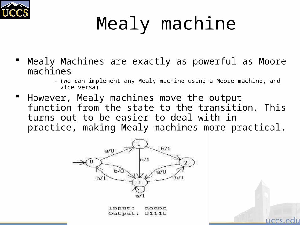
Mealy machine

Mealy Machines are exactly as powerful as Moore machines

– (we can implement any Mealy machine using a Moore machine, and vice versa).

However, Mealy machines move the output function from the state to the transition. This turns out to be easier to deal with in practice, making Mealy machines more practical.

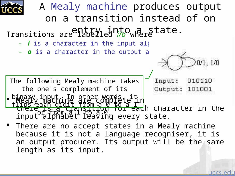
A Mealy machine produces output on a transition instead of on entry into a state.

Transitions are labelled i/o where – i is a character in the input alphabet and – o is a character in the output alphabet.

Mealy machine are complete in the sense that there is a transition for each character in the input alphabet leaving every state.

There are no accept states in a Mealy machine because it is not a language recogniser, it is an output producer. Its output will be the same length as its input.

The following Mealy machine takes the one's complement of its binary input. In other words, it flips each digit from a 0 to a 1 or from a 1 to a 0.

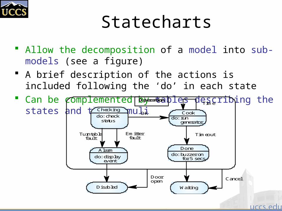
Statecharts

Allow the decomposition of a model into sub-models (see a figure) A brief description of the actions is included following the ‘do’ in

each state Can be complemented by tables describing the states and the

stimuliCook

do: run generator

Done

do: buzzer on for 5 secs.

Waiting

Alarm

do: display event

do: checkstatus

Checking

Turntablefault

Emitterfault

Disabled

OK

Timeout

TimeOperation

Dooropen

Cancel

Petri Nets Model

Petri Nets were developed originally by Carl Adam Petri, and were the subject of his dissertation in 1962.

Since then, Petri Nets and their concepts have been extended, developed, and applied in a variety of areas.

While the mathematical properties of Petri Nets are interesting and useful, the beginner will find that a good approach is to learn to model systems by constructing them graphically.

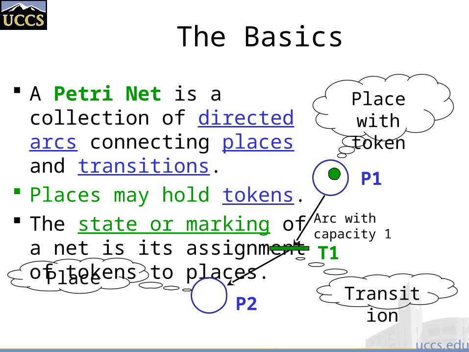
The Basics

A Petri Net is a collection of directed arcs connecting places and transitions.

Places may hold tokens. The state or marking of a net is

its assignment of tokens to places.

Place with token

P1

P2

T1

Arc with capacity 1

TransitionPlace

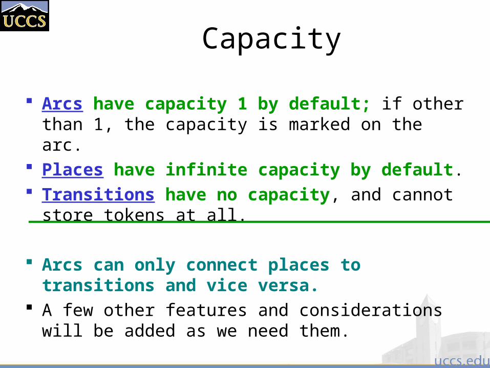
Capacity

Arcs have capacity 1 by default; if other than 1, the capacity is marked on the arc.

Places have infinite capacity by default. Transitions have no capacity, and cannot store

tokens at all.

Arcs can only connect places to transitions and vice versa.

A few other features and considerations will be added as we need them.

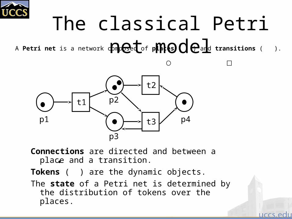
The classical Petri net modelA Petri net is a network composed of places ( ) and transitions ( ).

t2

p1

p2

p3

p4t3

t1

Connections are directed and between a place and a transition.

Tokens ( ) are the dynamic objects.

The state of a Petri net is determined by the distribution of tokens over the places.

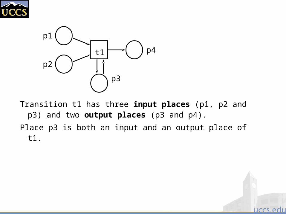
Transition t1 has three input places (p1, p2 and p3) and two output places (p3 and p4).

Place p3 is both an input and an output place of t1.

p1

p2

p3

p4t1

Enabling conditionTransitions are the active components and places and tokens are passive.

A transition is enabled if each of the input places contains tokens.

t1 t2

Transition t1 is not enabled, transition t2 is enabled.

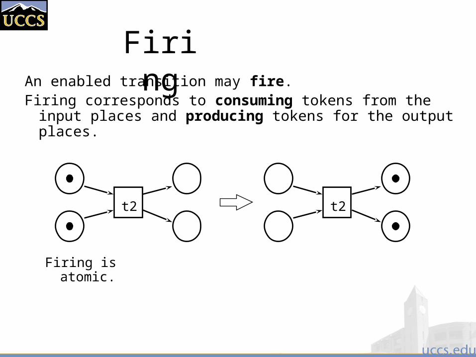
FiringAn enabled transition may fire.

Firing corresponds to consuming tokens from the input places and producing tokens for the output places.

t2t2

Firing is atomic.

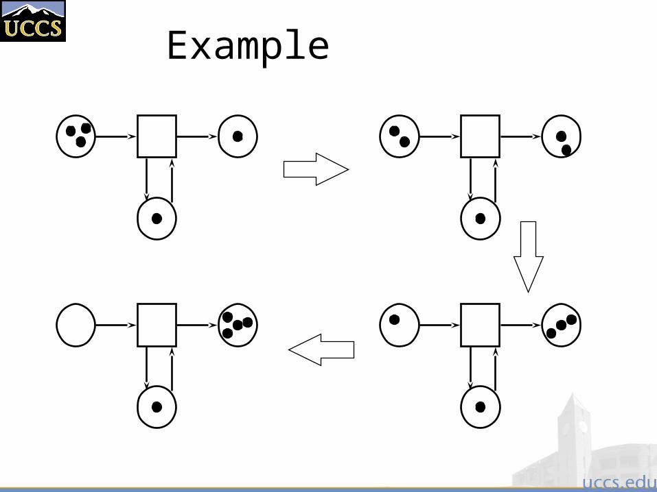
Example

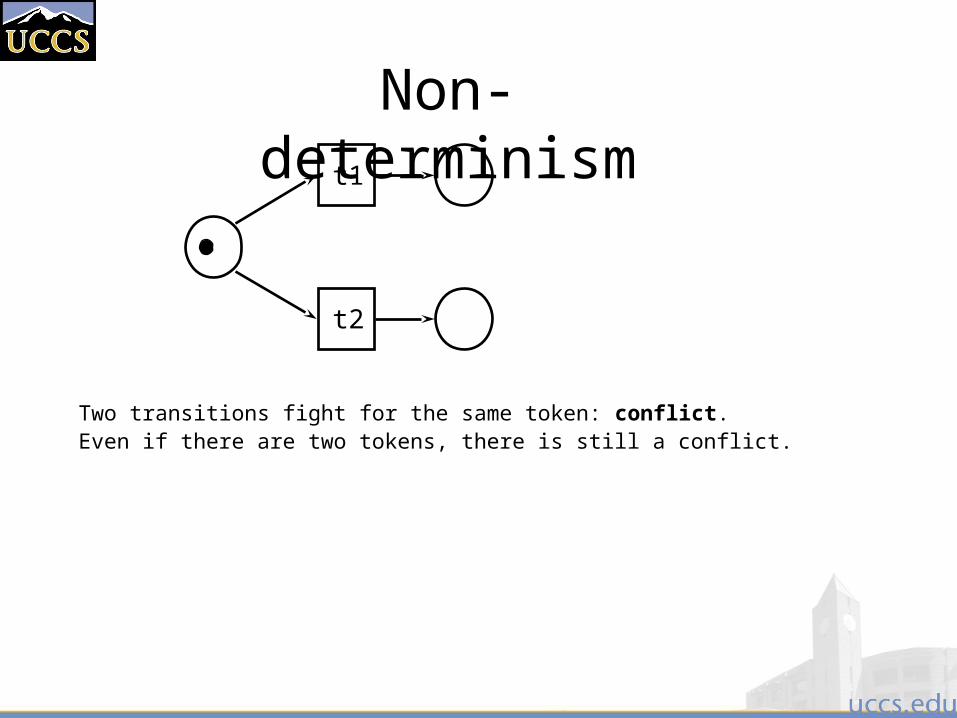
Non-determinism

Two transitions fight for the same token: conflict.Even if there are two tokens, there is still a conflict.

t1

t2

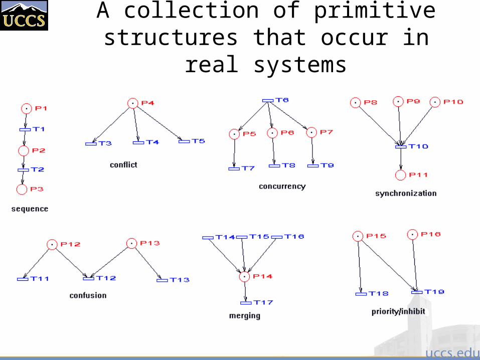
A collection of primitive structures that occur in real systems

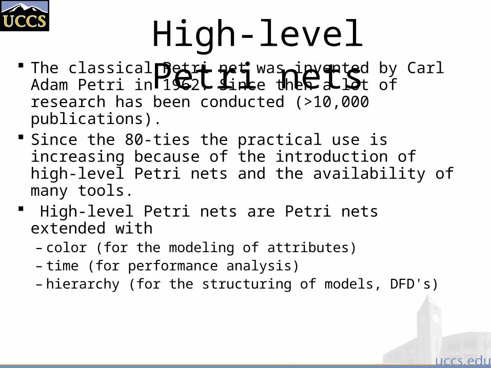
High-level Petri nets The classical Petri net was invented by Carl Adam

Petri in 1962. Since then a lot of research has been conducted (>10,000 publications).

Since the 80-ties the practical use is increasing because of the introduction of high-level Petri nets and the availability of many tools.

High-level Petri nets are Petri nets extended with– color (for the modeling of attributes)– time (for performance analysis)– hierarchy (for the structuring of models, DFD's)

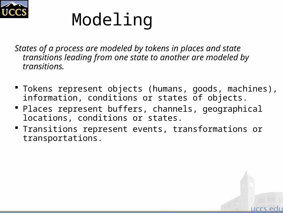
Modeling

States of a process are modeled by tokens in places and state transitions leading from one state to another are modeled by transitions.

Tokens represent objects (humans, goods, machines), information, conditions or states of objects.

Places represent buffers, channels, geographical locations, conditions or states.

Transitions represent events, transformations or transportations.

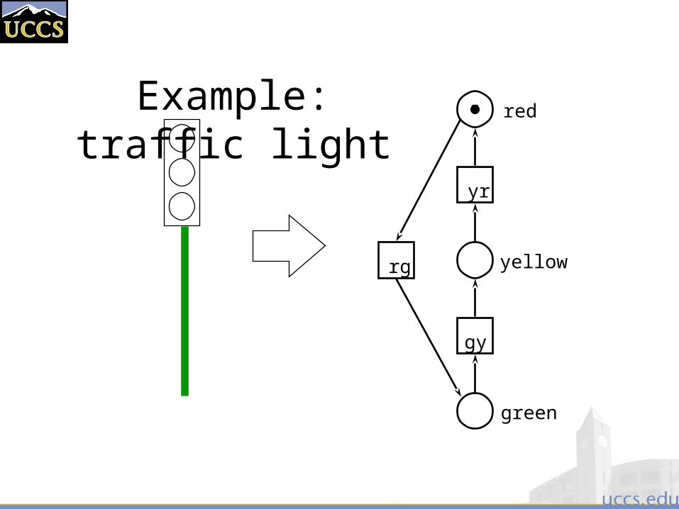
Example: traffic light

rg

red

yellow

green

yr

gy

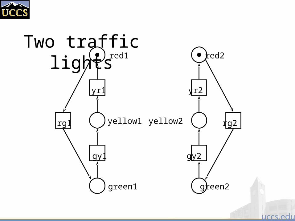
Two traffic lights

rg1

red1

yellow1

green1

yr1

gy1

rg2

red2

yellow2

green2

yr2

gy2

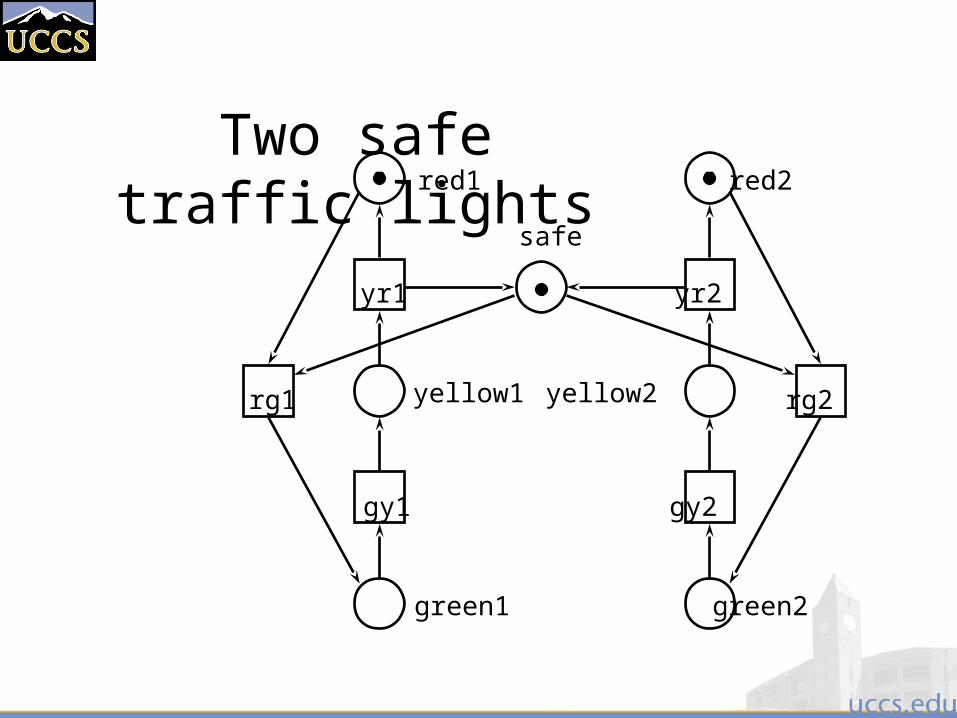
Two safe traffic lights

rg1

red1

yellow1

green1

yr1

gy1

rg2

red2

yellow2

green2

yr2

gy2

safe

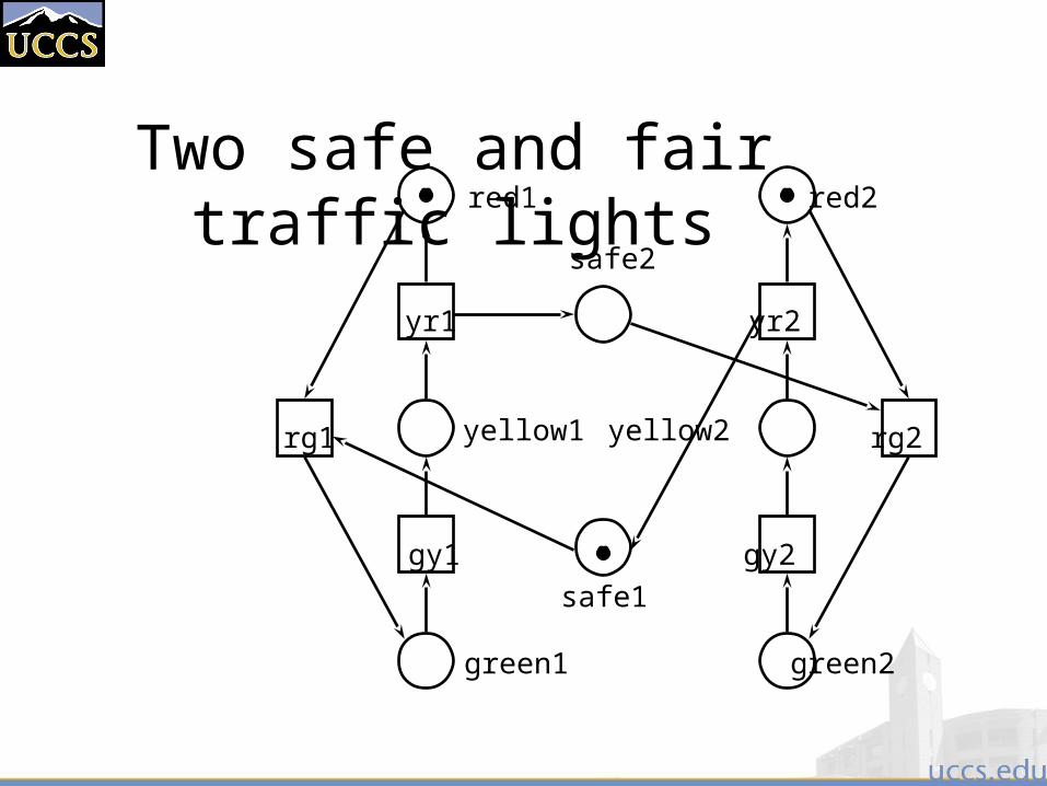
Two safe and fair traffic lights

rg1

red1

yellow1

green1

yr1

gy1

rg2

red2

yellow2

green2

yr2

gy2

safe2

safe1

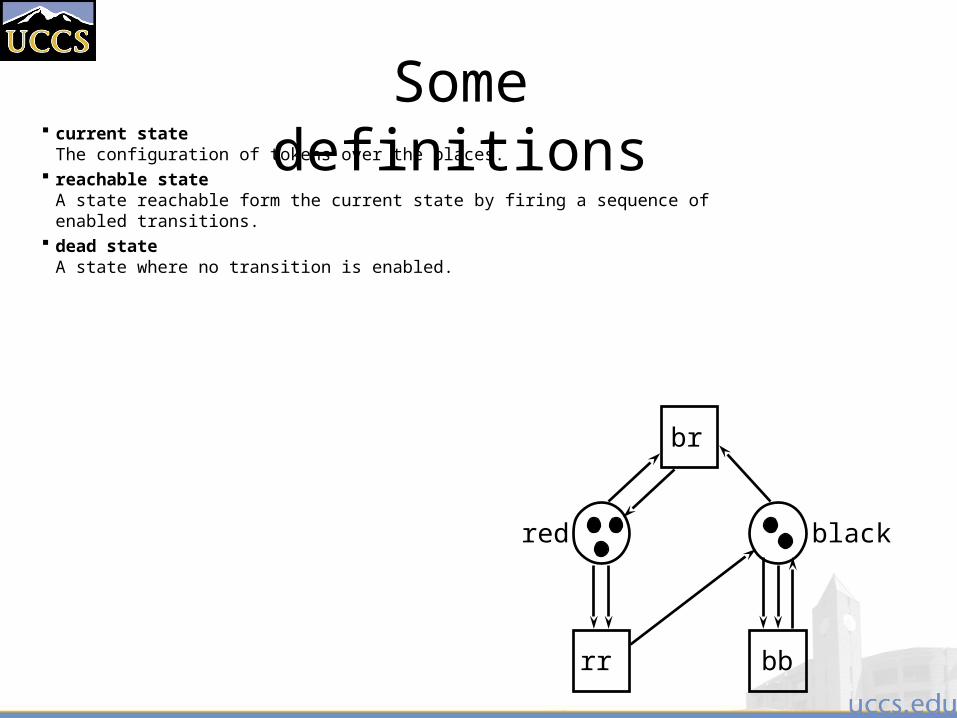
current stateThe configuration of tokens over the places.

reachable stateA state reachable form the current state by firing a sequence of enabled transitions.

dead stateA state where no transition is enabled.

Some definitions

blackred

bbrr

br

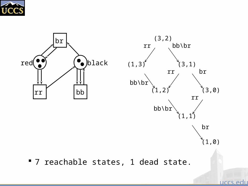
7 reachable states, 1 dead state.

blackred

bbrr

br (3,2)

(1,3) (3,1)

(1,2) (3,0)

(1,1)

(1,0)

rr

rr

rr

br

br

bb\br

bb\br

bb\br

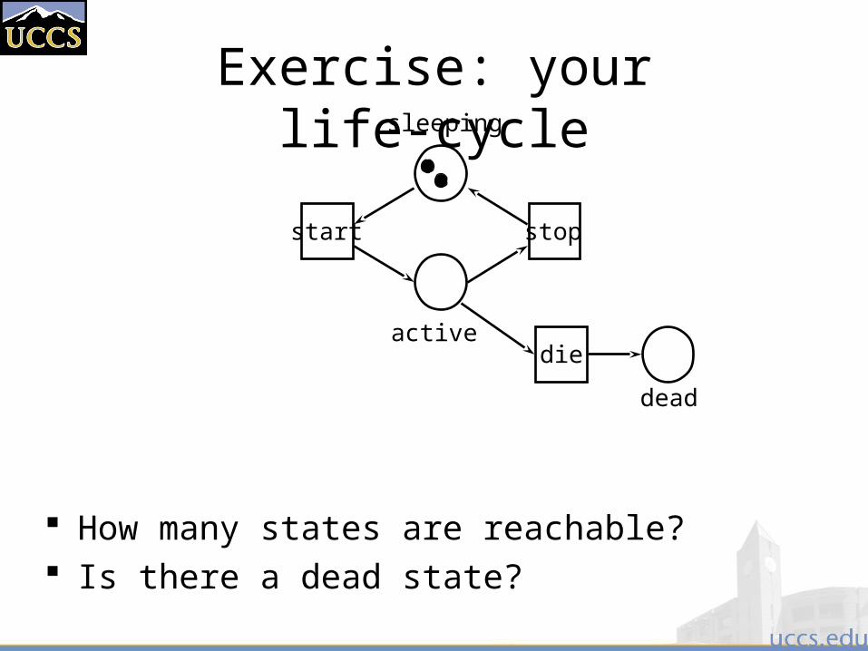
Exercise: your life-cycle

How many states are reachable? Is there a dead state?

dead

sleeping

active

start stop

die

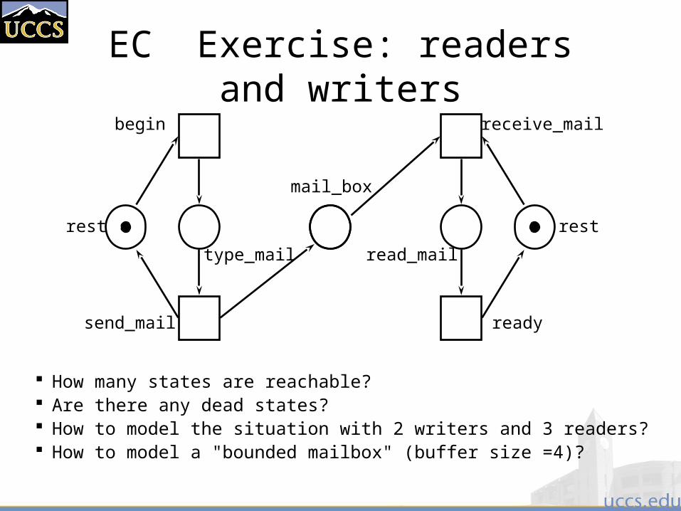
EC Exercise: readers and writers

How many states are reachable? Are there any dead states? How to model the situation with 2 writers and 3 readers? How to model a "bounded mailbox" (buffer size =4)?

rest

mail_box

receive_mail

type_mail

ready

rest

begin

send_mail

read_mail

High-level Petri nets

In practice the classical Petri net is not very useful: The Petri net becomes too large and too complex. It takes too much time to model a given situation. It is not possible to handle time and data.

Therefore, we use high-level Petri nets, i.e. Petri nets extended with:

color time hierarchy

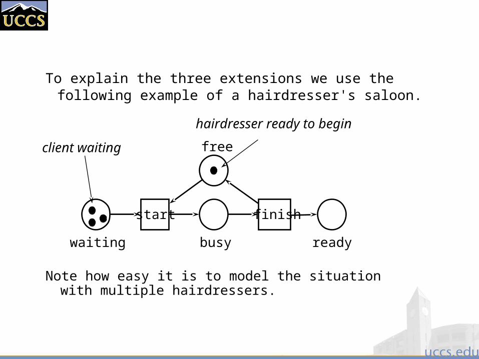
To explain the three extensions we use the following example of a hairdresser's saloon.

start

waiting

finish

busy

free

ready

client waiting

hairdresser ready to begin

Note how easy it is to model the situation with multiple hairdressers.

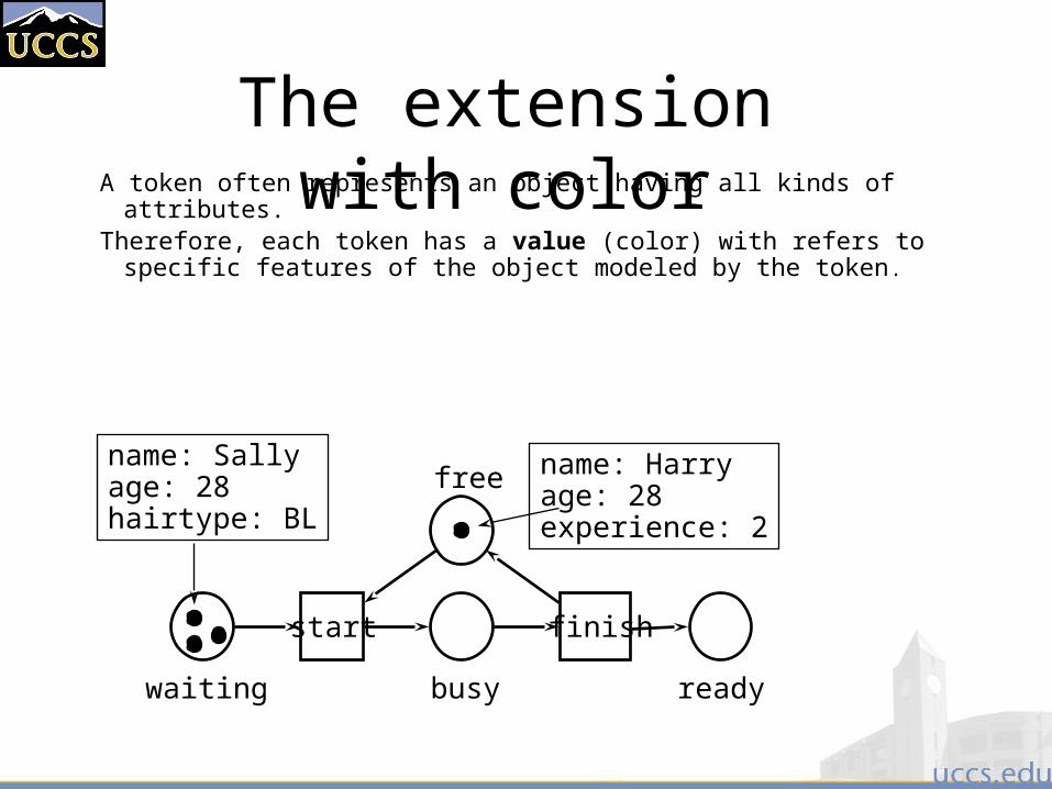
The extension with colorA token often represents an object having all kinds of attributes.

Therefore, each token has a value (color) with refers to specific features of the object modeled by the token.

start

waiting

finish

busy

free

ready

name: Harryage: 28experience: 2

name: Sallyage: 28hairtype: BL

Each transition has an (in)formal specification which specifies:

the number of tokens to be produced, the values of these tokens, and (optionally) a precondition.

The complexity is divided over the network and the values of tokens.

This results in a compact, manageable and natural process description.

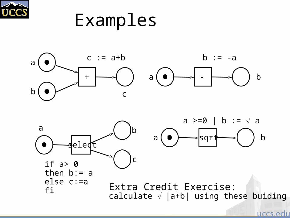
Examples

c := a+ba

b c

+

b := -a

b-a

if a> 0then b:= aelse c:=afi

a b

c

select

a >=0 | b := a

bsqrta

Extra Credit Exercise:calculate |a+b| using these buiding blocks

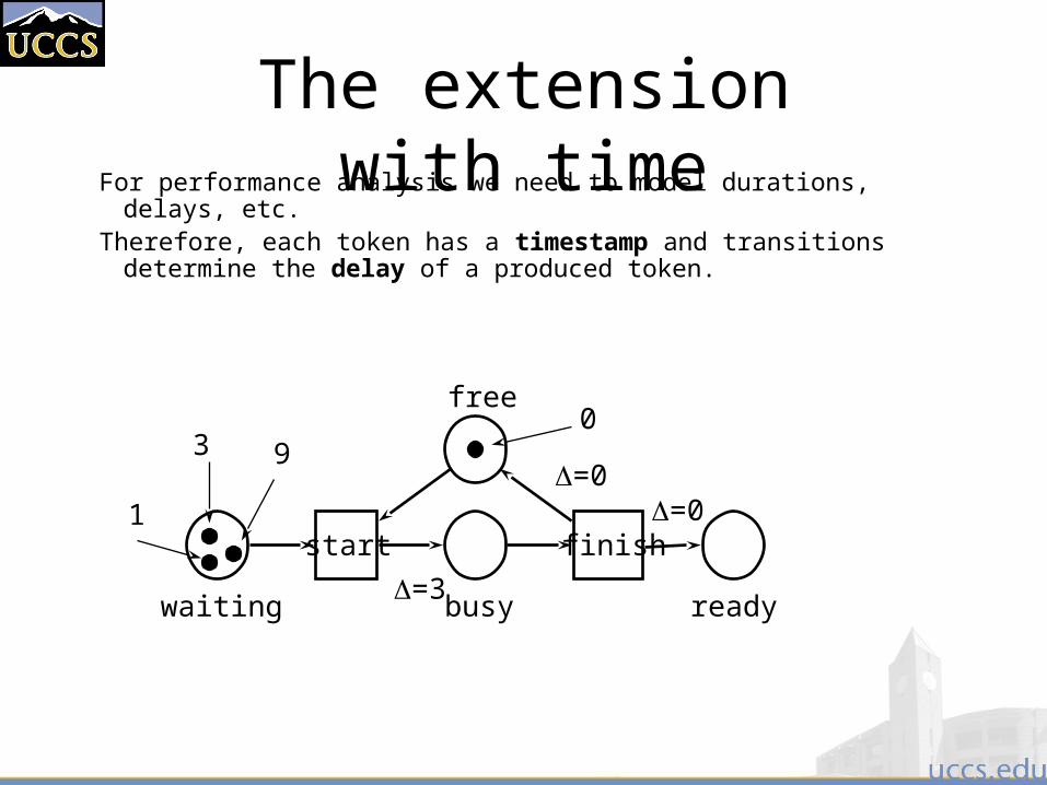
The extension with timeFor performance analysis we need to model durations, delays, etc.

Therefore, each token has a timestamp and transitions determine the delay of a produced token.

start

waiting

finish

busy

free

ready

0

1

3 9

=3

=0=0

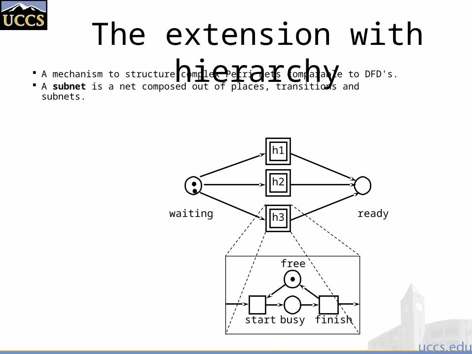
The extension with hierarchy A mechanism to structure complex Petri nets comparable to DFD's.

A subnet is a net composed out of places, transitions and subnets.

waiting ready

h1

h2

h3

start finishbusy

free

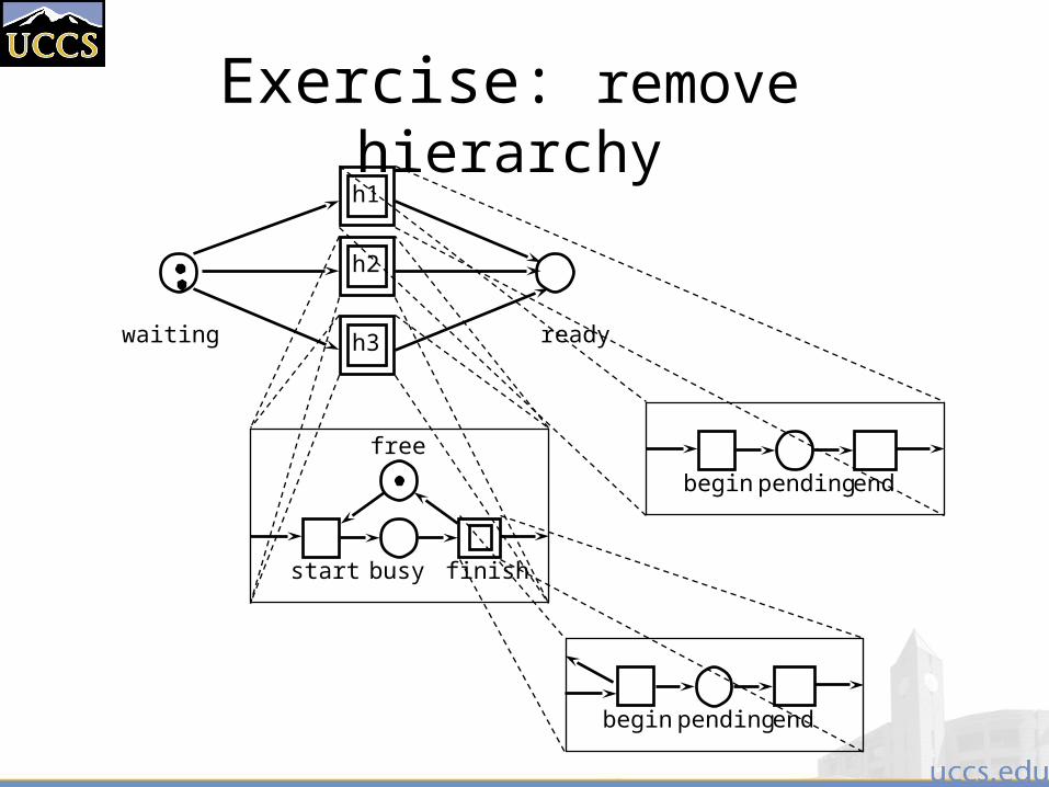
Exercise: remove hierarchy

waiting ready

h1

h2

h3

start finishbusy

free

begin endpending

begin endpending

Key points

Modeling specification complements informal requirements elicitation techniques.

Model specifications can be precise and unambiguous, but generally depend on interpretation of inputs/output. They reduce areas of doubt in a specification

More formal models, such as FSM or Petri nets forces an analysis of the system requirements at an early stage. Correcting errors at this stage is cheaper than modifying a system during design

Formal methods

Formal specification is part of a more general collection of techniques that are known as ‘formal methods’

These are all based on mathematical representation and analysis of software

Formal methods include– Formal specification– Specification analysis and proof– Transformational development– Program verification

Acceptance of formal methods

Formal methods have not become mainstream software development techniques as was once predicted– Other software engineering techniques have been successful

at increasing system quality. Hence the need for formal methods has been reduced

– Market changes have made time-to-market rather than software with a low error count the key factor. Formal methods do not reduce time to market

– The scope of formal methods is limited. They are not well-suited to specifying and analysing user interfaces and user interaction

– Formal methods are hard to scale up to large systems

Use of formal methods

Their principal benefits are in reducing the number of errors in systems so their main area of applicability is critical systems:– Air traffic control information systems,– Railway signalling systems– Spacecraft systems– Medical control systems

In this area, the use of formal methods is most likely to be cost-effective

Formal methods have limited practical applicability

Specification in the software process

Specification and design are inextricably mixed.

Architectural design is essential to structure a specification.

Formal specifications are expressed in a mathematical notation with precisely defined vocabulary, syntax and semantics.

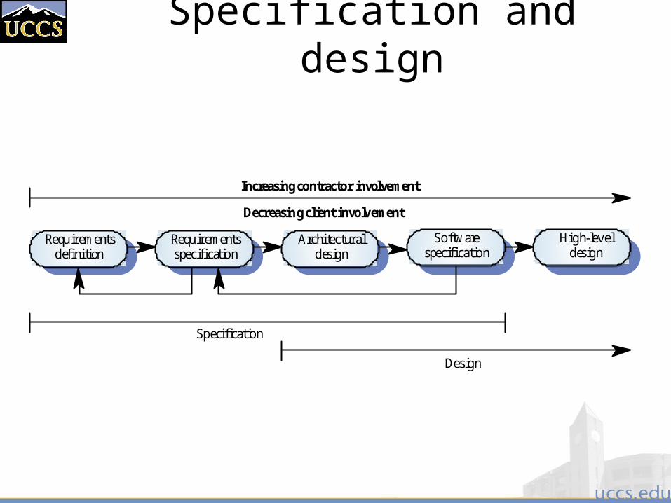
Specification and design

Architecturaldesign

Requirementsspecification

Requirementsdefinition

Softwarespecification

High-leveldesign

Increasing contractor involvement

Decreasing client involvement

Specification

Design

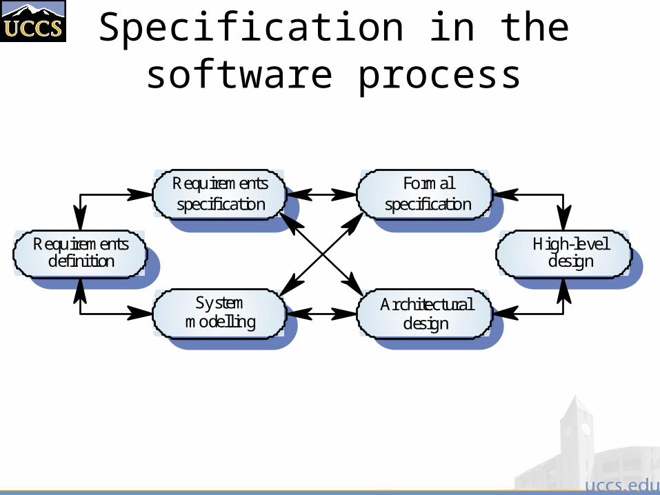
Specification in the software process

Requirementsspecification

Formalspecification

Systemmodelling

Architecturaldesign

Requirementsdefinition

High-leveldesign

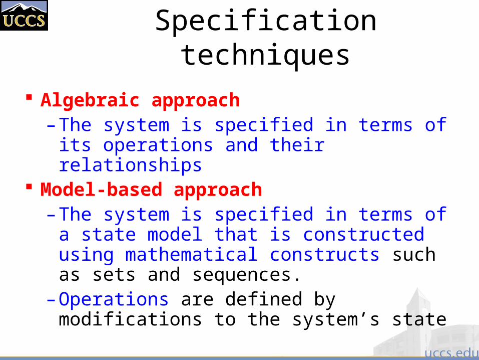
Specification techniques

Algebraic approach– The system is specified in terms of its

operations and their relationships Model-based approach

– The system is specified in terms of a state model that is constructed using mathematical constructs such as sets and sequences.

– Operations are defined by modifications to the system’s state

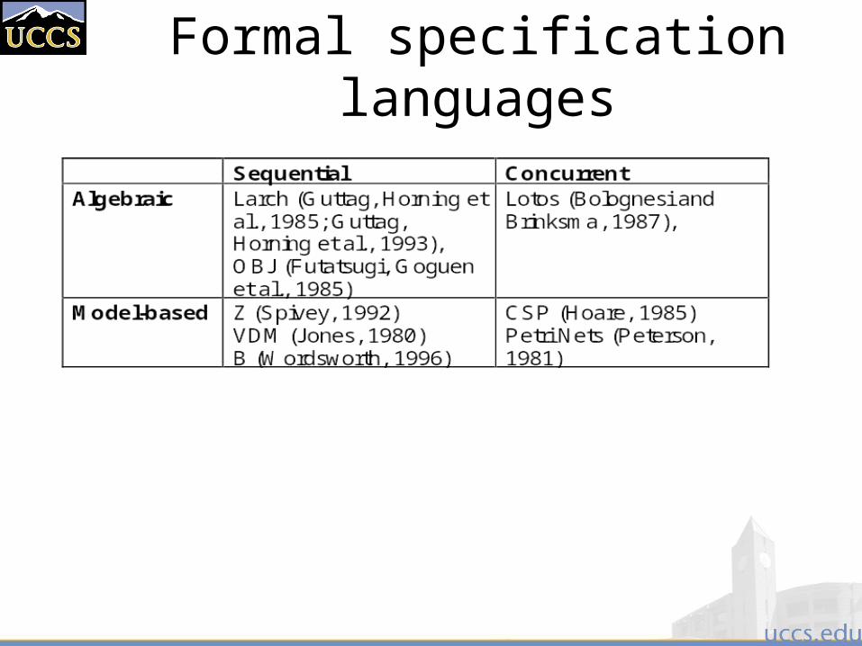
Formal specification languages

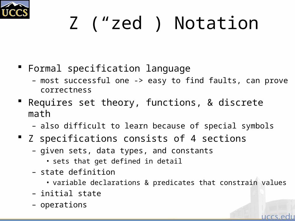
Z (“zed”) Notation

Formal specification language– most successful one -> easy to find faults, can prove correctness

Requires set theory, functions, & discrete math– also difficult to learn because of special symbols

Z specifications consists of 4 sections– given sets, data types, and constants

• sets that get defined in detail

– state definition• variable declarations & predicates that constrain values

– initial state

– operations

Use of formal specification

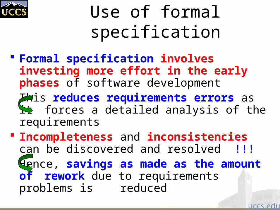
Formal specification involves investing more effort in the early phases of software development

This reduces requirements errors as it forces a detailed analysis of the requirements

Incompleteness and inconsistencies can be discovered and resolved !!!

Hence, savings as made as the amount of rework due to requirements problems is reduced

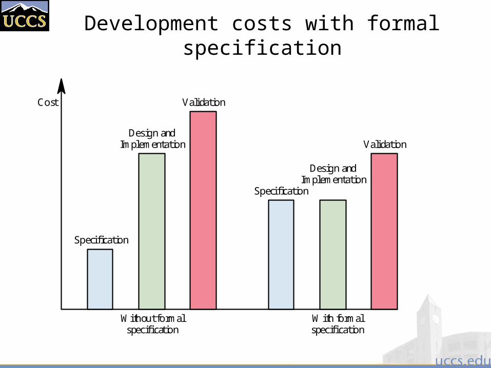
Development costs with formal specification

Specification

Design andImplementation

Validation

Specification

Design andImplementation

Validation

Cost

Without formalspecification

With formalspecification

1. Interface specification

Large systems are decomposed into subsystems with well-defined interfaces between these subsystems

Specification of subsystem interfaces allows independent development of the different subsystems

Interfaces may be defined as abstract data types or object classes

The algebraic approach to formal specification is particularly well-suited to interface specification

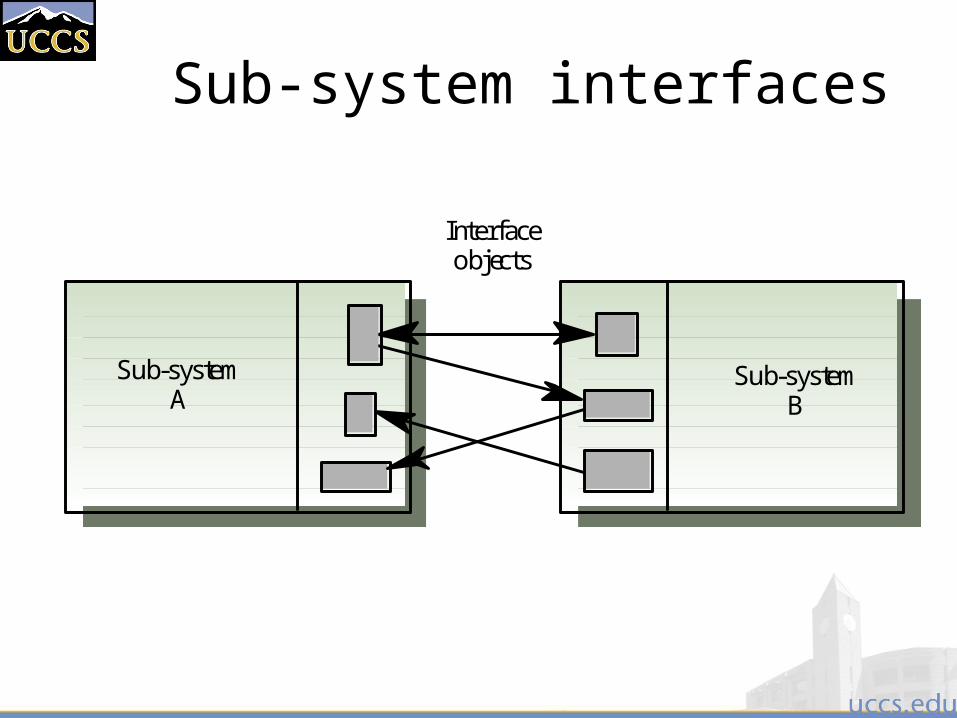
Sub-system interfaces

Sub-systemA

Sub-systemB

Interfaceobjects

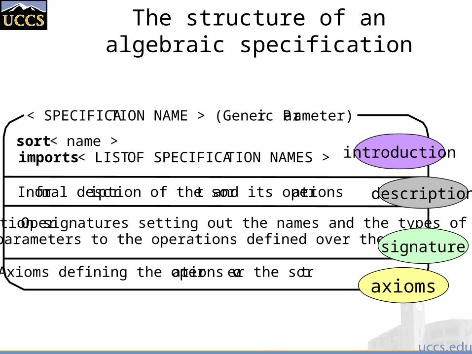
The structure of an algebraic specification

sort < name >imports < LIST OF SPECIFICATION NAMES >

Informal descr iption of the sor t and its operations

Operation signatures setting out the names and the types ofthe parameters to the operations defined over the sort

Axioms defining the operations over the sort

< SPECIFICATION NAME > (Gener ic Parameter)

introduction

description

signature

axioms

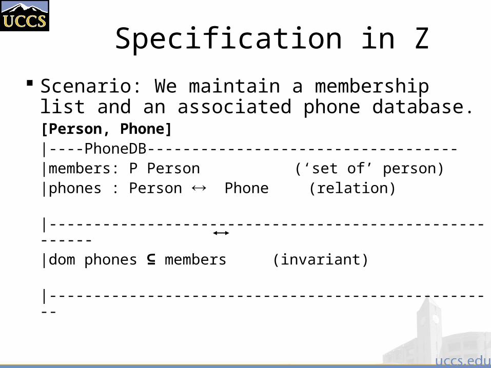
Specification in Z

Scenario: We maintain a membership list and an associated phone database.[Person, Phone]|----PhoneDB-----------------------------------|members: P Person (‘set of’ person)|phones : Person Phone (relation)|-------------------------------------------------------|dom phones ⊆ members (invariant)|---------------------------------------------------

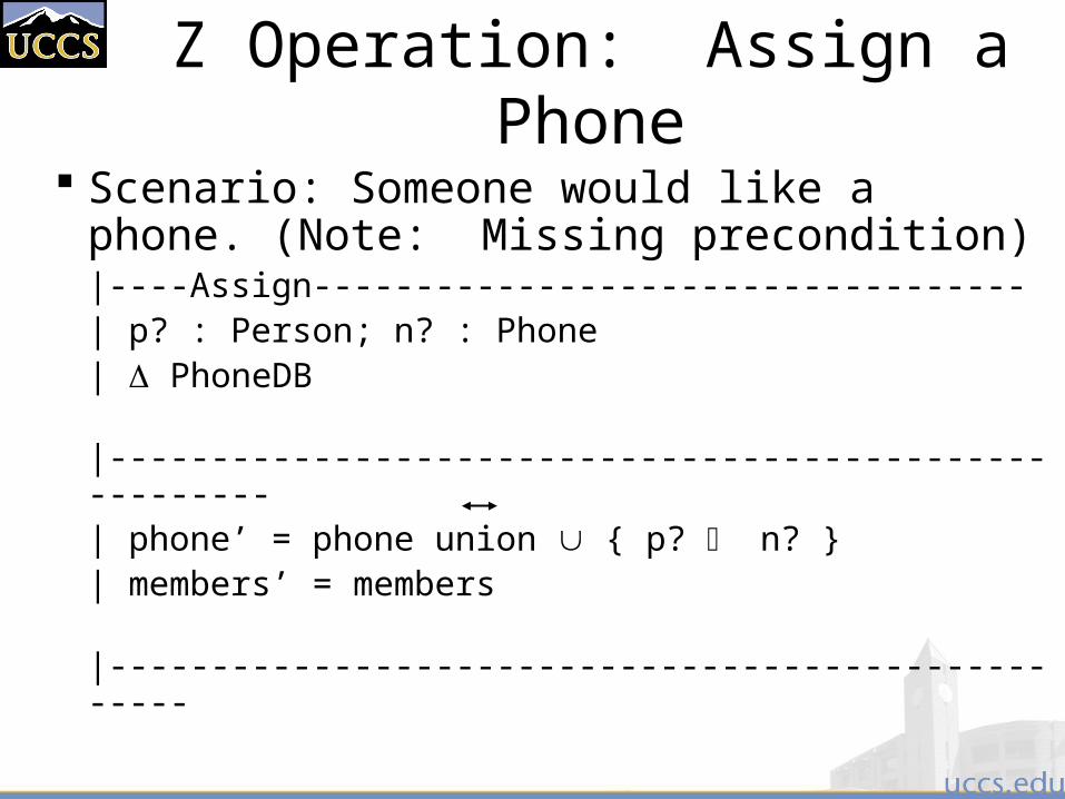
Z Operation: Assign a Phone

Scenario: Someone would like a phone. (Note: Missing precondition)|----Assign-----------------------------------| p? : Person; n? : Phone| PhoneDB|-------------------------------------------------------| phone’ = phone union { p? n? }| members’ = members|---------------------------------------------------

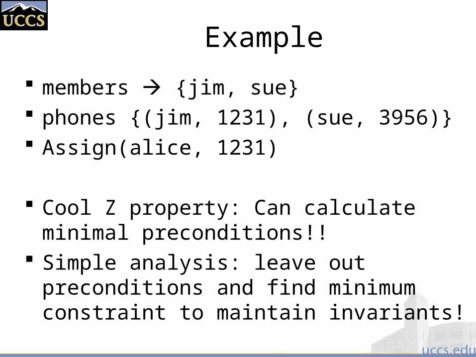
Example

members {jim, sue} phones {(jim, 1231), (sue, 3956)} Assign(alice, 1231)

Cool Z property: Can calculate minimal preconditions!!

Simple analysis: leave out preconditions and find minimum constraint to maintain invariants!

Behavioural specification

Algebraic specification can be cumbersome when the object operations are not independent of the object state

Model-based specification exposes the system state and defines the operations in terms of changes to that state

Abstract State Machine Language (AsmL)

AsmL is a language for modelling the structure and behaviour of digital systems

AsmL can be used to faithfully capture the abstract structure and step-wise behaviour of any discrete systems, including very complex ones such as:Integrated circuits, software components, and devices that combine both hardware and software

Abstract State

An AsmL model is said to be abstract because it encodes only those aspects of the system’s structure that affect the behaviour being modelled

The goal is to use the minimum amount of detail that accurately reproduces (or predicts) the

behaviour of the system Abstraction helps us reduce complex problems into

manageable units and prevents us from getting lost in a sea of details

AsmL provides a variety of features that allow you to describe the relevant state of a

system in a very economical, high-level way

Abstract State Machine and Turing Machine

An abstract state machine is a particular kind of mathematical machine, like the Turing machine (TM)

But unlike a TM, ASMs may be defined a very high level of abstraction

An easy way to understand ASMs is to see them as defining a succession of states that may follow an initial state

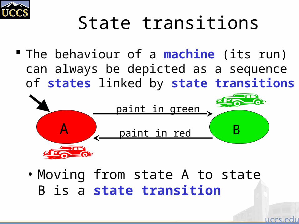
State transitions

The behaviour of a machine (its run) can always be depicted as a sequence of states linked by state transitions

• Moving from state A to state B is a state transition

paint in green

paint in redA B

Configurations

Each state is a particular “configuration” of the machine

The state may be simple or it may be very large, with complex structure

But no matter how complex the state might be, each step of the machine’s operation can be seen as a well-defined transition from one particular state to another

Evolution of state variables

paint in green

paint in redA B

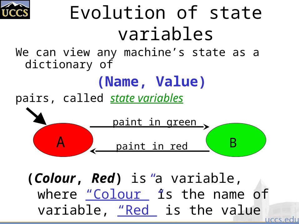
We can view any machine’s state as a dictionary of

(Name, Value) pairs, called state variables

(Colour, Red) is a variable, where “Colour” is the name of variable, “Red” is the value

Evolution of state variables

Names are given by the machine’s symbolic vocabulary

Values are fixed elements, like numbers and strings of characters

The run of a machine is a series of

states and state transitions that

results form applying operations

to each state in succession

Example

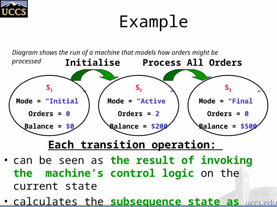
Diagram shows the run of a machine that models how orders might be processed

S1

Mode = “Initial”

Orders = 0

Balance = $0

Initialise Process All Orders

S3

Mode = “Final”

Orders = 0

Balance = $500

S2

Mode = “Active”

Orders = 2

Balance = $200

Each transition operation: • can be seen as the result of invoking the machine’s

control logic on the current state • calculates the subsequence state as output

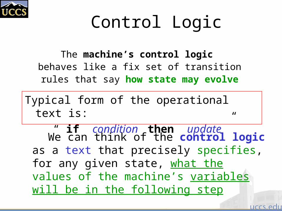
Control Logic

The machine’s control logic behaves like a fix set of transition

rules that say how state may evolve

We can think of the control logic as a text that precisely specifies, for any given state, what the values of the machine’s variables will be in the following step

Typical form of the operational text is:

“ if condition then update ”

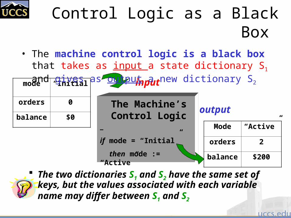
Control Logic as a Black Box

The two dictionaries S1 and S2 have the same set of keys, but the values associated with each variable name may differ between S1 and S2

The Machine’s Control Logic

…

if mode = “Initial”

then mode := “Active”

mode “Initial”

orders 0

balance $0

Mode “Active”

orders 2

balance $200

input

output

• The machine control logic is a black box that takes as input a state dictionary S1 and gives as output a new dictionary S2

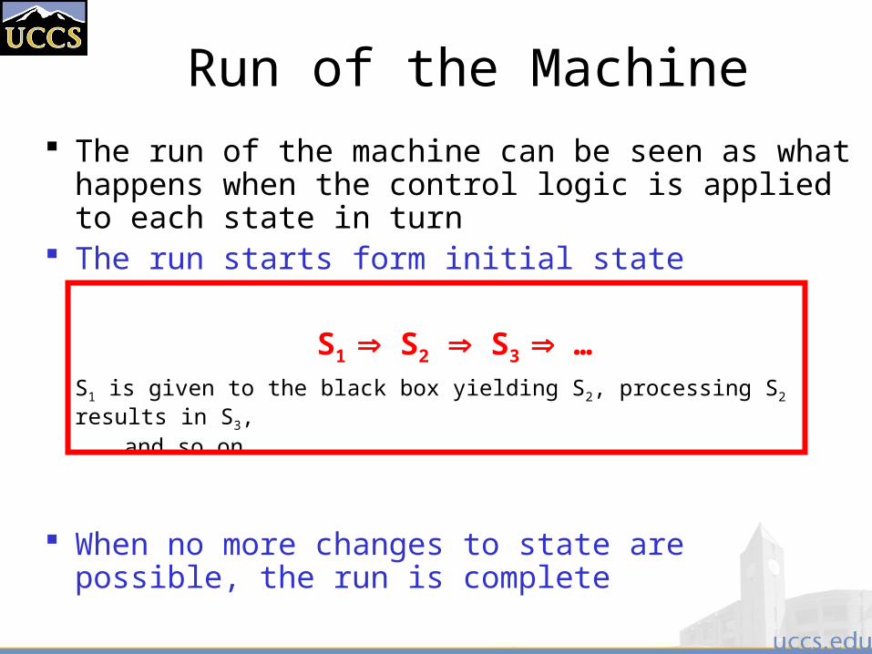
Run of the Machine

The run of the machine can be seen as what happens when the control logic is applied to each state in turn

The run starts form initial state

S1 S2 S3 …S1 is given to the black box yielding S2, processing S2 results in S3,

and so on …

When no more changes to state are possible, the run is complete

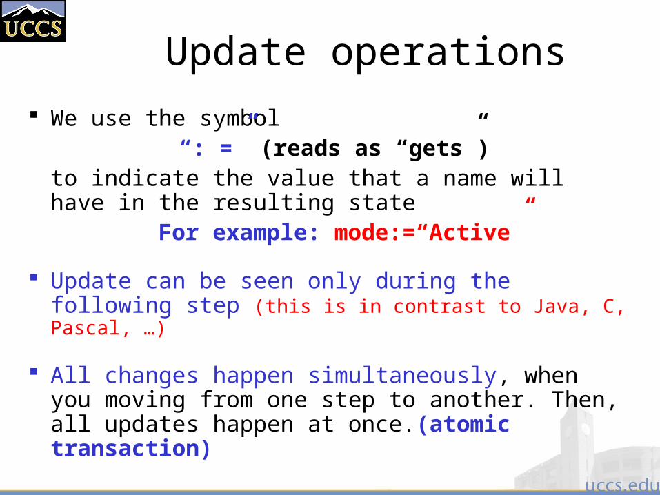
Update operations

We use the symbol “: =” (reads as “gets”)

to indicate the value that a name will have in the resulting state

For example: mode:=“Active”

Update can be seen only during the following step (this is in contrast to Java, C, Pascal, …)

All changes happen simultaneously, when you moving from one step to another. Then, all updates happen at once.(atomic transaction)

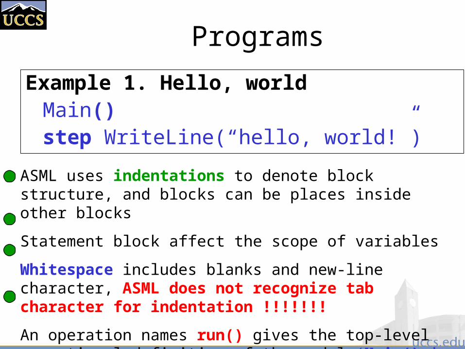
Programs

Example 1. Hello, worldMain()

step WriteLine(“hello, world!”)

ASML uses indentations to denote block structure, and blocks can be places inside other blocks

Statement block affect the scope of variables

Whitespace includes blanks and new-line character, ASML does not recognize tab character for indentation !!!!!!!

An operation names run() gives the top-level operational definition of the model (Main() is like main() in Java and C )

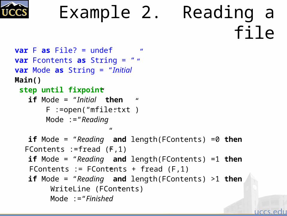
Example 2. Reading a file

var F as File? = undefvar Fcontents as String = “”var Mode as String = “Initial”Main() step until fixpoint if Mode = “Initial” then F :=open(“mfile.txt”) Mode :=“Reading”

if Mode = “Reading” and length(FContents) =0 then FContents :=fread (F,1)

if Mode = “Reading” and length(FContents) =1 then FContents := FContents + fread (F,1)

if Mode = “Reading” and length(FContents) >1 then WriteLine (FContents) Mode :=“Finished”

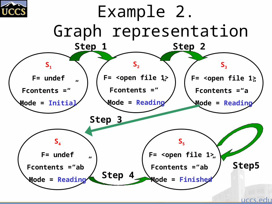
Example 2. Graph representation

S1

F= undef

Fcontents =“”

Mode = Initial

Step 1 Step 2

S3

F= <open file 1>

Fcontents =“a”

Mode = Reading

S2

F= <open file 1>

Fcontents =“”

Mode = Reading

S4

F= undef

Fcontents =“ab”

Mode = Reading Step 4Step5

S5

F= <open file 1>

Fcontents =“ab”

Mode = Finished

Step 3

Key points

Formal system specification complements informal specification and modeling techniques

Formal specifications are precise and unambiguous. They remove areas of doubt in a specification, but still depend on interpretation of terms, inputs and outputs.

Formal specification forces an very details analysis of the system requirements at an early stage. Correcting errors at this stage is cheaper.

Key points Formal specification techniques are most applicable in

the development of critical systems and standards. Algebraic techniques are suited to interface specification

where the interface is defined as a set of object classes Model-based techniques model the system using sets and

functions. This simplifies some types of behavioural specification

Its not for the faint of heart, you’ll need some special training to go down this path.