smith chart

9/24/2012

1

JBC © 1982~2009 Telecommunications

JBCardenas © 1982

Transmission Media and Antenna Transmission Media and Antenna Systems Part IISystems Part II

Sources:Com3 Lecture NotesFValiente’s Com3 2011 presentation slidesJCardenas’ Com4/Com5 2011 presentation slidesCarr, Practical Antenna Handbook, TAB, 1989Tomasi, Connor ECSE2100 lecture RPI 2004

http://www.maxim-ic.com/appnotes.cfm/appnote_number/742/ http://www.ece.uvic.ca/~whoefer/elec454/Lecture%2004.pdf http://www.sss-mag.com/smith.htmlhttp://www.educatorscorner.com/index.http://www.amanogawa.com/index.html

Excerpts of presentation materials, not in MIT Lecture Notes

2012 © Jose Cardenas, v 1.0

Excerpts of presentation materials, not in MIT Lecture Notes

2012 © Jose Cardenas, v 1.0

JBC © 198 v A1.05 Telecommunications

JBCardenas © 1982

SC Movie-Lectures

Movies• Intro Male• Intro Female• Reflection coefficient• Transmission coefficient• Open and Short Circuits• Input Impedance• Load Impedance• VSWR Vmax Vmin• Slotted Line• Matching• Antenna• Summary

These and other on-line sources• www.antenna-theory.com• ‘ECE3300’• Others….

9/24/2012

2


JBCardenas © 1982

Topic 05Students and presenters should have sample charts, ruler,

compass and colored pens. Presenter: get a giant compass, a giant ruler

Basics of Smith Charts, more on the chart than historyPlot impedances and admittances

Get reflection coefficients, transmission coefficients, VSWRFind SWR, | | , resistive load

Find Zi of a shorted or open line of length L

SOLVE FOR LENGHTFind Zi of a line terminated with ZL

SOLVE FOR LENGHT


JBCardenas © 1982

The Smith chart, named after Phillip Hagar Smith, is a graphical aid to solving transmission-line impedance problems and to illustrate how RF parameters behave at given frequencies; still usedl for antenna problems and equipment displays

Two Smith Charts samples are shown below:• Green: admitance (+ below)• Red: impedance• Combined: immittance

The Smith Chart

9/24/2012

3


JBCardenas © 1982

Smith Chart Applications

• Smith charts can be used to represent parameters such as impedances, admittances, transmission coefficients (scattering parameters), noise figure circles, constant gain contours, Q contours, regions of unconditional stability, etc…

• It is the graphical equivalent (geometry) to mathematical calculations using complex algebra to match ladder networks to T.L. for example.

• Applications to be discussed in this course:– Find SWR, | |∠ , RL– Find YL

– Find Zi of a shorted or open line of length l– Find Zi of a line terminated with ZL– Find distance to Vmax and Vmin from ZL

– Solution for quarter-wave transformer matching– Solution for parallel series single-stub matching


JBCardenas © 1982

Smith Chart Basics• The coordinates on the chart are based on the intersection of two sets of

orthogonal circles.• One set represents the normalized resistive component, r (= R/Zo), tangent

to a point on the right side of the outer circle along the center horizontal line

Open circuitShort circuit

9/24/2012

4


JBCardenas © 1982

+j0.7

-j1.4

j0

Smith Chart Basics

• The other set is the normalized reactive component, ± jx (= ± jX/Zo), tangent to the same point but rotated 90 º clockwise or counter clockwise.

+


JBCardenas © 1982Smith Chart Basics

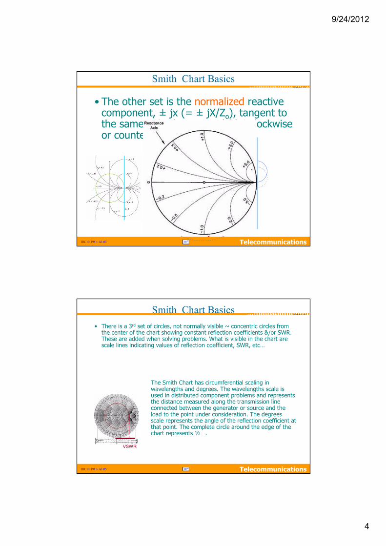
• There is a 3rd set of circles, not normally visible ~ concentric circles from the center of the chart showing constant reflection coefficients &/or SWR. These are added when solving problems. What is visible in the chart are scale lines indicating values of reflection coefficient, SWR, etc…

The Smith Chart has circumferential scaling in wavelengths and degrees. The wavelengths scale is used in distributed component problems and represents the distance measured along the transmission line connected between the generator or source and the load to the point under consideration. The degrees scale represents the angle of the reflection coefficient at that point. The complete circle around the edge of the chart represents ½ .

VSWR

9/24/2012

5


JBCardenas © 1982

Plotting Points on the Smith Chart

• Define Normalized Impedance

• Reflection Coefficient in terms of zL

Note: this keeps values w/in range on S.C.

L L L0 0

L L LZ R jXz r jxZ Z

+≡ = ≡ +

L 0 0 L

L 0 0 L

1/ 11/ 1

Z Z Z zZ Z Z z

− −Γ= = + +


JBCardenas © 1982

r = 1

r = 2

+j0.7

-j1.4

z1

z2

z1 = 1+j0.7

z2 = 2-j1.4

Example

• Plot the following:

9/24/2012

6


JBCardenas © 1982

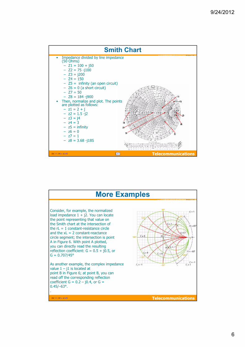
Smith Chart • Impedance divided by line impedance

(50 Ohms)– Z1 = 100 + j50 – Z2 = 75 -j100 – Z3 = j200 – Z4 = 150 – Z5 = infinity (an open circuit)– Z6 = 0 (a short circuit)– Z7 = 50 – Z8 = 184 -j900

• Then, normalize and plot. The points are plotted as follows:– z1 = 2 + j– z2 = 1.5 -j2– z3 = j4– z4 = 3– z5 = infinity– z6 = 0– z7 = 1– z8 = 3.68 -j18S


JBCardenas © 1982

More Examples

Consider, for example, the normalizedload impedance 1 + j2. You can locatethe point representing that value onthe Smith chart at the intersection ofthe rL = 1 constant-resistance circleand the xL = 2 constant-reactancecircle segment; the intersection is pointA in Figure 6. With point A plotted,you can directly read the resultingreflection coefficient: G = 0.5 + j0.5, orG = 0.707/45°

As another example, the complex impedancevalue 1 – j1 is located atpoint B in Figure 6; at point B, you canread off the corresponding reflectioncoefficient G = 0.2 – j0.4, or G =0.45/–63°..

9/24/2012

7


JBCardenas © 1982

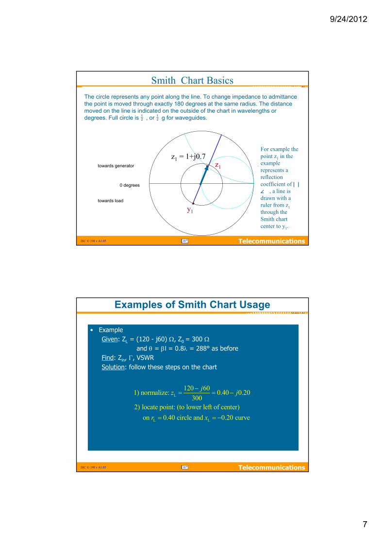
The circle represents any point along the line. To change impedance to admittance the point is moved through exactly 180 degrees at the same radius. The distance moved on the line is indicated on the outside of the chart in wavelengths or degrees. Full circle is 1 , or 1 g for waveguides.

z1 z1 = 1+j0.7

y1

0 degrees

towards generator

towards load

Smith Chart Basics

For example the point z1 in the example represents a reflection coefficient of | |∠∠∠∠ , a line is drawn with a ruler from z1through the Smith chart center to y1.

z1 = 1+j0.7


JBCardenas © 1982

Examples of Smith Chart Usage

• ExampleGiven: ZL = (120 - j60) Ω, Z0 = 300 Ω

and θ = βl = 0.8λ = 288° as before Find: Zin, Γ, VSWRSolution: follow these steps on the chart

L

L L

120 601) normalize: 0.40 0.20300

2) locate point: (to lower left of center) on 0.40 circle and 0.20 curve

jz j

r x

−= = −

= = −

9/24/2012

8


JBCardenas © 1982

Examples of Smith Chart Usage

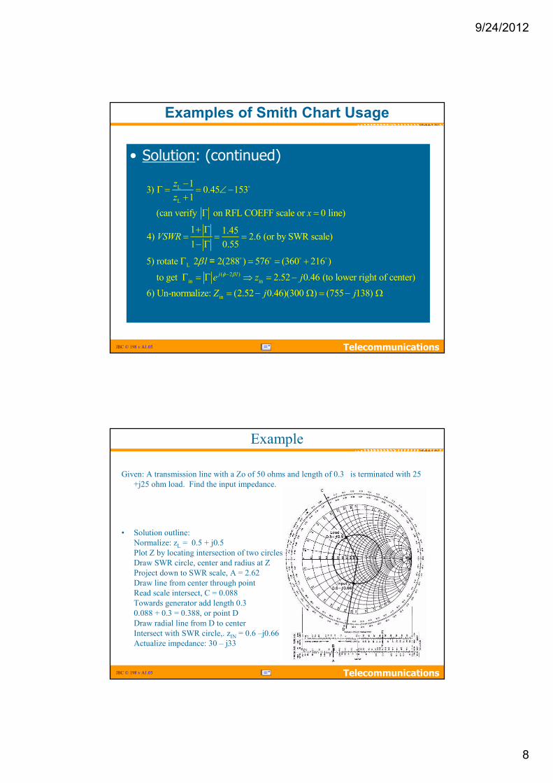
• Solution: (continued)

L

L

L( 2 )

in in

13) 0.45 153 1

(can verify on RFL COEFF scale or 0 line)

1 1.454) 2.6 (or by SWR scale)1 0.55

5) rotate 2 2(288 ) 576 (360 216 )

to get 2.52 0.46j l

zz

x

VSWR

le z jφ β

β−

−Γ = = ∠−

+

Γ =

+ Γ= = =

− Γ

Γ = = +

Γ = Γ ⇒ = −

o

o o o o=

in

(to lower right of center)6) Un-normalize: (2.52 0.46)(300 ) (755 138) Z j j= − Ω = − Ω


JBCardenas © 1982

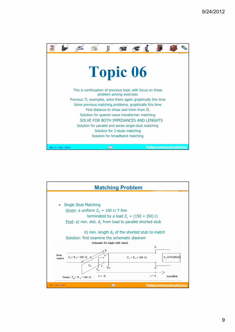
Given: A transmission line with a Zo of 50 ohms and length of 0.3 is terminated with 25 +j25 ohm load. Find the input impedance.

• Solution outline:Normalize: zL = 0.5 + j0.5Plot Z by locating intersection of two circlesDraw SWR circle, center and radius at ZProject down to SWR scale, A = 2.62Draw line from center through pointRead scale intersect, C = 0.088 Towards generator add length 0.3 0.088 + 0.3 = 0.388, or point DDraw radial line from D to centerIntersect with SWR circle,. zIN = 0.6 –j0.66Actualize impedance: 30 – j33

Example

9/24/2012

9


JBCardenas © 1982

Topic 06This is continuation of previous topic with focus on these

problem solving exercisesPrevious TL examples, solve them again graphically this time

Solve previous matching problems, graphically this timeFind distance to Vmax and Vmin from ZL

Solution for quarter-wave transformer matching

SOLVE FOR BOTH IMPEDANCES AND LENGHTSSolution for parallel and series single-stub matching

Solution for 2-stubs matchingSolution for broadband matching


JBCardenas © 1982

Matching Problem

• Single Stub MatchingGiven: a uniform Z0 = 100 Ω T-line

terminated by a load ZL = (150 + j50) ΩFind: a) min. dist. d1 from load to parallel shorted stub

b) min. length d2 of the shorted stub to matchSolution: first examine the schematic diagram

9/24/2012

10


JBCardenas © 1982

Single Stub Matching

• Solution: take the following steps on S.C.

L

L L2 ( / 4)

in 2 ( / 4)

Lin L

150 501) Normalize the load: 1.5 0.50100

2) Convert to admittance: 1/ 0.60 0.20

1 1Note: ( / 4)1 11 1 11 (0)

going halfway ( /4) around

j j

j j

jz j

y z je ez le e

yz z

β λ π

β λ πλ

λ

− −

− −

+= = +

= = −

+Γ +Γ− = − = =

−Γ −Γ−Γ

= = = =+Γ

∴ the smith chart converts any impedance to its reciprocal (admittance)!


JBCardenas © 1982



L

1

B B

3) Find the intersection between 0.27( 1.78) circle and the 1 circle

Note that two intersection points exist, but one minimizes the length . In terms of admittance

1.0 0.58

VSWR g

dy j g j

Γ =

= =

⇒ = + = + B

1 B A' (0.647 0.454) 0.193b

d z z λ λ∴ = − = − =

9/24/2012

11


JBCardenas © 1982



in B 0

ssss

inss C B

4) Find the minimum length of a shorted stub, that when inserted in parallel at B, produces a match ( ).

1 (exists at the right extreme)

Desire: 0 0.58

Z Z R

yzy y jb j

= =

= =∞

= = − = −

C

2 C ss

2

This occurs at the pos. on the S.C.: 0.416(0.416 0.250) 0.166

5) Adding the shorted stub of length in parallel at B completes our path on the S. C. from B to C (HOME!).

zd z z

d

λλ λ

=∴ = − = − =


JBCardenas © 1982

Single stub matching: move along the transmission line to rotate the mismatch to the unity resistance (conductance) circle and insert the appropriate type and length of stub in series (shunt) with the main line to move along this circle to the origin.

Example

• Example: add a stub in parallel with a transmission line

Solution: use an admittance chart because, at the attachment point, the resulting admittance is the sum of the stub's input susceptance and the main line admittance.

The mismatched point is rotated around the origin until it reaches the unity conductance circle.

The characteristic impedance and length of the stub is chosen such that its input susceptance is equal and opposite to the main line susceptance indicated on the unity conductance circle.

9/24/2012

12


JBCardenas © 1982

The example shows two cases: move toward the generator 39 degrees of line and add a short-circuited stub that provides 0.8 siemens normalized inductive susceptance, or move toward the generator 107 degrees of line and add an open-circuited stub that provides 0.8 siemens normalized capacitive susceptance.

•

Answer


JBCardenas © 1982

9/24/2012

13


JBCardenas © 1982

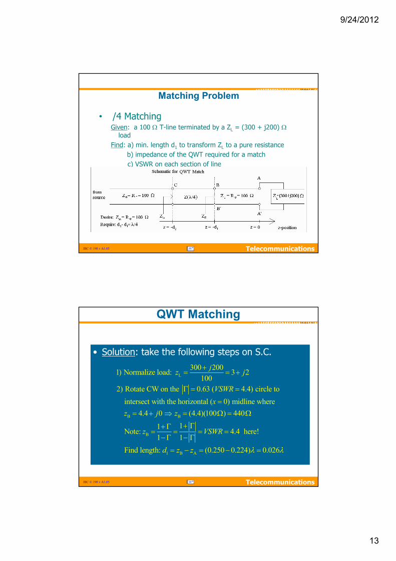
Matching Problem

• /4 MatchingGiven: a 100 Ω T-line terminated by a ZL = (300 + j200) Ω

loadFind: a) min. length d1 to transform ZL to a pure resistance

b) impedance of the QWT required for a matchc) VSWR on each section of line

Solution: first examine the schematic diagram


JBCardenas © 1982

QWT Matching

• Solution: take the following steps on S.C.

L

B B

B

300 2001) Normalize load: 3 2100

2) Rotate CW on the 0.63 ( 4.4) circle to intersect with the horizontal ( 0) midline where 4.4 0 (4.4)(100 ) 440

11 Note: 1 1

jz j

VSWRx

z j z

z

+= = +

Γ = =

== + ⇒ = Ω = Ω

+ Γ+Γ= = =

−Γ − Γ

1 B A

4.4 here!

Find length: (0.250 0.224) 0.026

VSWR

d z z λ λ

=

= − = − =

9/24/2012

14


JBCardenas © 1982

QWT Matching


BB'

3) Find ( / 4) for a match with 100 line:

( 4) (440 )(100 ) 210440 then re-normalize on the QWT to get 2.09

( / 4) 2104) Rotate CW on the 0.36 ( 2.09) circle halfway ( 4)

Z

Z λ/zz

zVSWR

λ/

λ

Ω

= Ω Ω = Ω

Ω= = =

Ω

Γ = =

C C

0 0

D

around the chart to input of the QWT where 0.48 0 and (0.48)(210 ) 100.85) Now re-normalize on the 100Ω line to get 1.0 at D (we have arrived at HOME for a match!)

z j ZZ R

z VSWR

= + = Ω = Ω

= == =


JBCardenas © 1982

Other Applications using SC

Q and Broadband Matching Computer Aids are Available

Antenna Zo vs Freq NEC

smith chart

Documents

Transcript of smith chart