Smith Chart - Amanogawaamanogawa.com/archive/docs/G-tutorial.pdf · Smith Chart The Smith chart is...

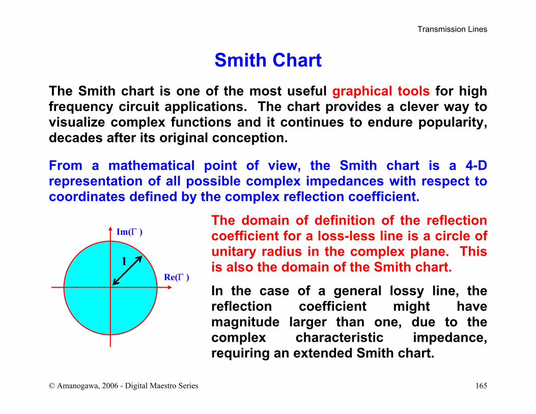
Transmission Lines

© Amanogawa, 2006 - Digital Maestro Series 165

Smith Chart The Smith chart is one of the most useful graphical tools for high frequency circuit applications. The chart provides a clever way to visualize complex functions and it continues to endure popularity, decades after its original conception.

From a mathematical point of view, the Smith chart is a 4-D representation of all possible complex impedances with respect to coordinates defined by the complex reflection coefficient.

The domain of definition of the reflection coefficient for a loss-less line is a circle of unitary radius in the complex plane. This is also the domain of the Smith chart.

In the case of a general lossy line, the reflection coefficient might have magnitude larger than one, due to the complex characteristic impedance, requiring an extended Smith chart.

Im(Γ )

Re(Γ )1

Transmission Lines


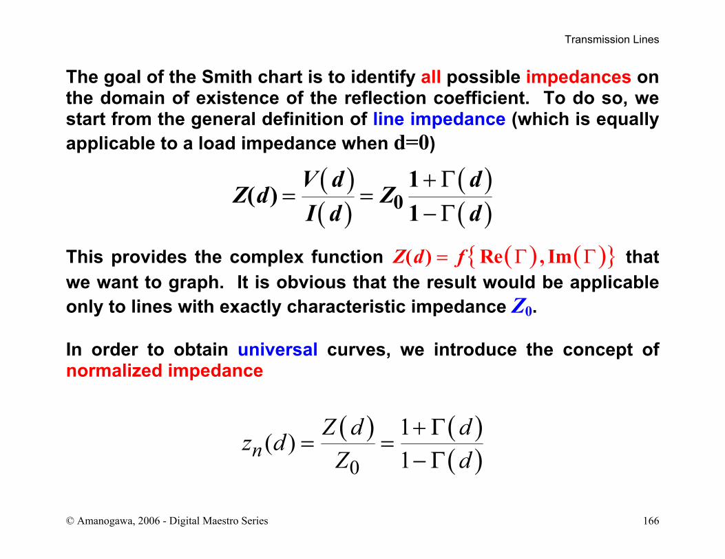
The goal of the Smith chart is to identify all possible impedances on the domain of existence of the reflection coefficient. To do so, we start from the general definition of line impedance (which is equally applicable to a load impedance when d=0)

( )( )

( )( )0

1( )

1V d d

Z d ZI d d

+ Γ= =

− Γ

This provides the complex function ( ) ( ) ( ) Re , ImZ d f= Γ Γ that we want to graph. It is obvious that the result would be applicable only to lines with exactly characteristic impedance Z0. In order to obtain universal curves, we introduce the concept of normalized impedance

( ) ( )( )0

1( )1n

Z d dz dZ d

+ Γ= =

− Γ

Transmission Lines


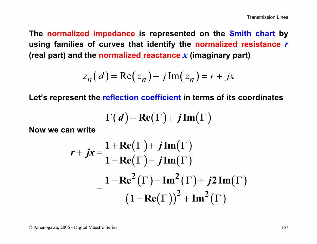
The normalized impedance is represented on the Smith chart by using families of curves that identify the normalized resistance r (real part) and the normalized reactance x (imaginary part)

( ) ( ) ( )Re Imn n nz d z j z r jx= + = + Let’s represent the reflection coefficient in terms of its coordinates

( ) ( ) ( )Re Imd jΓ = Γ + Γ Now we can write

( ) ( )( ) ( )

( ) ( ) ( )( )( ) ( )

2 2

2 2

1 Re Im1 Re Im

1 Re Im 2 Im

1 Re Im

jr jx

j

j

+ Γ + Γ+ =

− Γ − Γ

− Γ − Γ + Γ=

− Γ + Γ

Transmission Lines


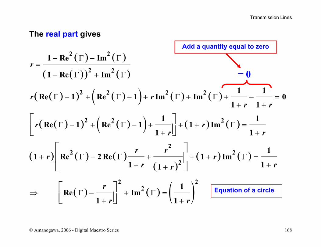
The real part gives

( ) ( )

( )( ) ( )

( )( ) ( )( ) ( ) ( )

( )( ) ( )( ) ( ) ( )

( ) ( ) ( )( )

( ) ( )

( ) ( ) ( )

2 2

2 2

2 2 2 2

2 2 2

22 2

2

2 22

1 Re Im

1 Re Im

1 1Re 1 Re 1 Im Im 0

1 1

1 1Re 1 Re 1 1 Im

1 1

11 Re 2 Re 1 Im

1 11

1Re Im

1 1

r

r rr r

r rr r

r rr r

r rr

r

r r

− Γ − Γ=

− Γ + Γ

Γ − + Γ − + Γ + Γ + − =+ +

Γ − + Γ − + + + Γ =+ +

+ Γ − Γ + + + Γ =+ ++

⇒ Γ − + Γ =+ +

= 0

Add a quantity equal to zero

Equation of a circle

Transmission Lines


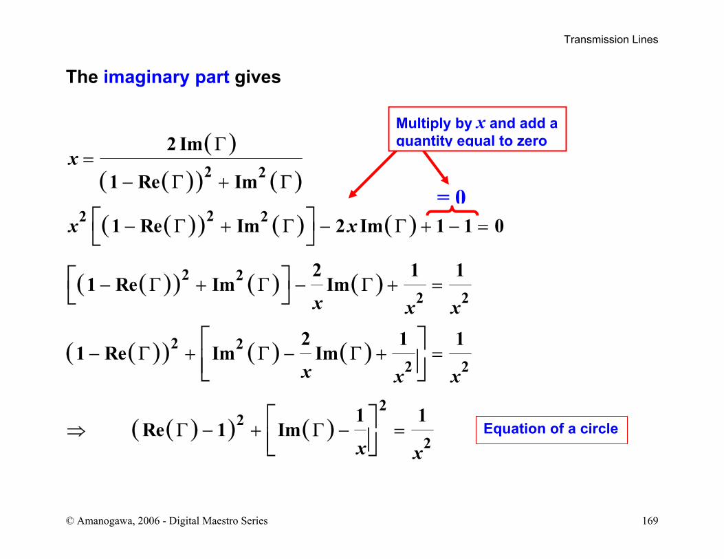
The imaginary part gives

( )( )( ) ( )

( )( ) ( ) ( )

( )( ) ( ) ( )

( )( ) ( ) ( )

( )( ) ( )

2 2

22 2

2 22 2

2 22 2

22

2

2 Im

1 Re Im

1 Re Im 2 Im 1 1 0

2 1 11 Re Im Im

2 1 11 Re Im Im

1 1Re 1 Im

x

x x

x x x

x x x

x x

Γ=

− Γ + Γ

− Γ + Γ − Γ + − =

− Γ + Γ − Γ + =

− Γ + Γ − Γ + =

⇒ Γ − + Γ − =

= 0

Multiply by x and add a quantity equal to zero

Equation of a circle

Transmission Lines


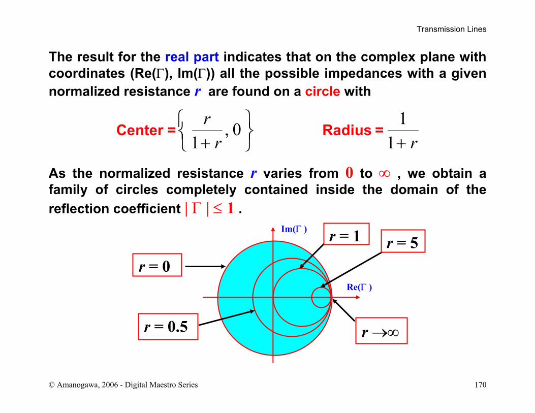
The result for the real part indicates that on the complex plane with coordinates (Re(Γ), Im(Γ)) all the possible impedances with a given normalized resistance r are found on a circle with

1, 01 1rr r

+ +

Center = Radius =

As the normalized resistance r varies from 0 to ∞ , we obtain a family of circles completely contained inside the domain of the reflection coefficient | Γ | ≤ 1 .

Im(Γ )

Re(Γ )

r = 0

r →∞

r = 1

r = 0.5

r = 5

Transmission Lines


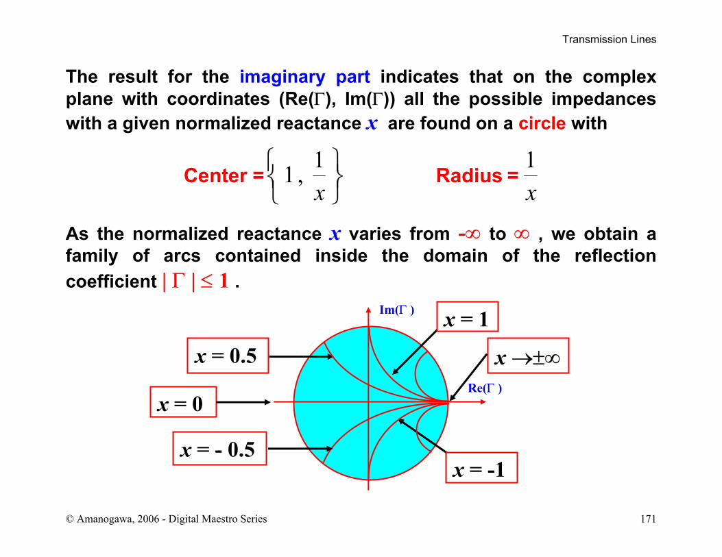
The result for the imaginary part indicates that on the complex plane with coordinates (Re(Γ), Im(Γ)) all the possible impedances with a given normalized reactance x are found on a circle with

1 11,x x

Center = Radius =

As the normalized reactance x varies from -∞ to ∞ , we obtain a family of arcs contained inside the domain of the reflection coefficient | Γ | ≤ 1 .

Im(Γ )

Re(Γ )x = 0

x →±∞

x = 1

x = 0.5

x = -1x = - 0.5

Transmission Lines


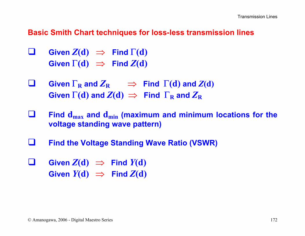
Basic Smith Chart techniques for loss-less transmission lines

Given Z(d) ⇒ Find Γ(d) Given Γ(d) ⇒ Find Z(d)

Given ΓR and ZR ⇒ Find Γ(d) and Z(d)

Given Γ(d) and Z(d) ⇒ Find ΓR and ZR

Find dmax and dmin (maximum and minimum locations for the voltage standing wave pattern)

Find the Voltage Standing Wave Ratio (VSWR)

Given Z(d) ⇒ Find Y(d)

Given Y(d) ⇒ Find Z(d)

Transmission Lines


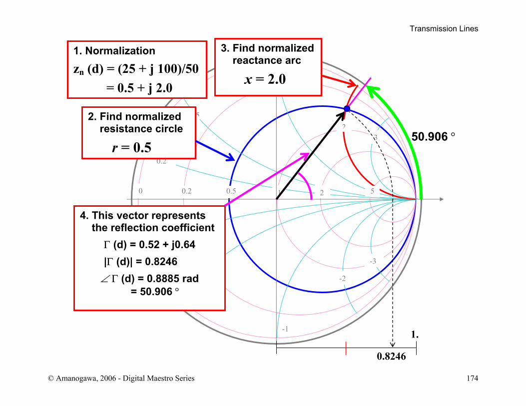
Given Z(d) ⇒ Find Γ(d) 1. Normalize the impedance

( ) ( )0 0 0

ddnZ R Xz j r j xZ Z Z

= = + = +

2. Find the circle of constant normalized resistance r 3. Find the arc of constant normalized reactance x 4. The intersection of the two curves indicates the reflection

coefficient in the complex plane. The chart provides directly the magnitude and the phase angle of Γ(d)

Example: Find Γ(d), given

( ) 0d 25 100 with 50Z j Z= + Ω = Ω

Transmission Lines


1

-1

0 0.2 0.5 5

0.2

-0.2

21

-0 5

0 5

-3

32

-2

1. Normalization

zn (d) = (25 + j 100)/50 = 0.5 + j 2.0

2. Find normalized resistance circle

r = 0.5

3. Find normalized reactance arc

x = 2.0

4. This vector represents the reflection coefficient

Γ (d) = 0.52 + j0.64 |Γ (d)| = 0.8246

∠ Γ (d) = 0.8885 rad = 50.906 °

50.906 °

1.

0.8246

Transmission Lines


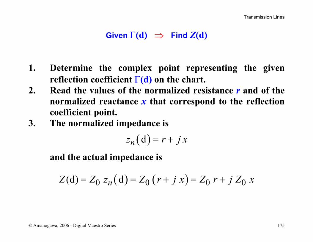
Given Γ(d) ⇒ Find Z(d) 1. Determine the complex point representing the given

reflection coefficient Γ(d) on the chart. 2. Read the values of the normalized resistance r and of the

normalized reactance x that correspond to the reflection coefficient point.

3. The normalized impedance is

( )dnz r j x= +

and the actual impedance is

( ) ( )0 0 0 0(d) dnZ Z z Z r j x Z r j Z x= = + = +

Transmission Lines


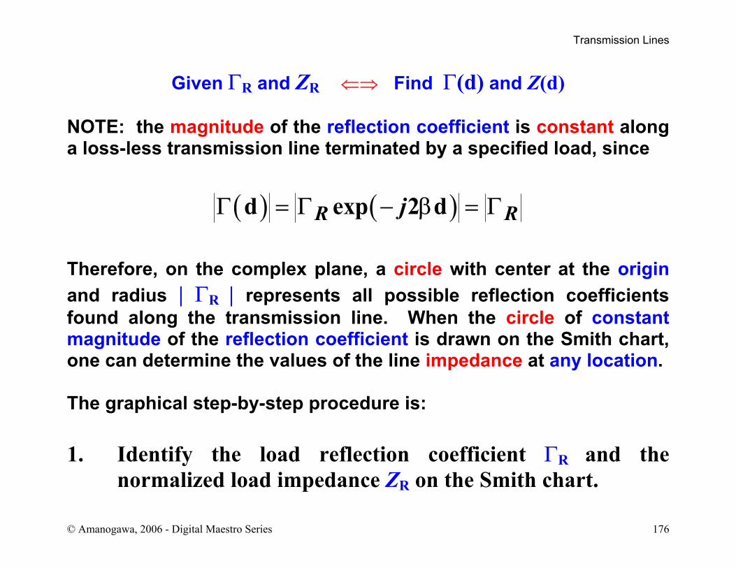
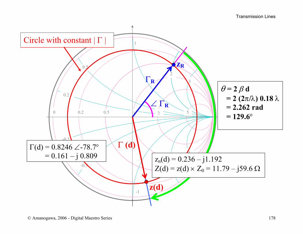
Given ΓR and ZR ⇐⇒ Find Γ(d) and Z(d) NOTE: the magnitude of the reflection coefficient is constant along a loss-less transmission line terminated by a specified load, since

( ) ( )d exp 2 dR RjΓ = Γ − β = Γ

Therefore, on the complex plane, a circle with center at the origin and radius | ΓR | represents all possible reflection coefficients found along the transmission line. When the circle of constant magnitude of the reflection coefficient is drawn on the Smith chart, one can determine the values of the line impedance at any location. The graphical step-by-step procedure is: 1. Identify the load reflection coefficient ΓR and the

normalized load impedance ZR on the Smith chart.

Transmission Lines


2. Draw the circle of constant reflection coefficient amplitude |Γ(d)| =|ΓR|.

3. Starting from the point representing the load, travel on the circle in the clockwise direction, by an angle

22 d 2 dπθ = β =

λ

4. The new location on the chart corresponds to location d on the transmission line. Here, the values of Γ(d) and Z(d) can be read from the chart as before.

Example: Given

025 100 50RZ j Z= + Ω = Ωwith

find

( ) ( ) 0.18Z d d dΓ = λand for

Transmission Lines


θ

1

-1

0 0.2 0.5 5

0.2

-0.2

21

-0.5

0.5

-3

32

-2

ΓR

zR

∠ ΓR

θ = 2 β d = 2 (2π/λ) 0.18 λ = 2.262 rad = 129.6°

z(d)

Γ (d)Γ(d) = 0.8246 ∠-78.7° = 0.161 – j 0.809 zn(d) = 0.236 – j1.192

Z(d) = z(d) × Z0 = 11.79 – j59.6 Ω

Circle with constant | Γ |

Transmission Lines


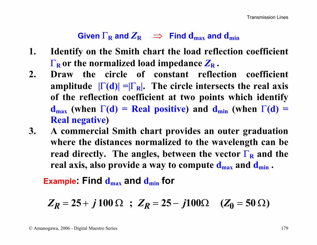
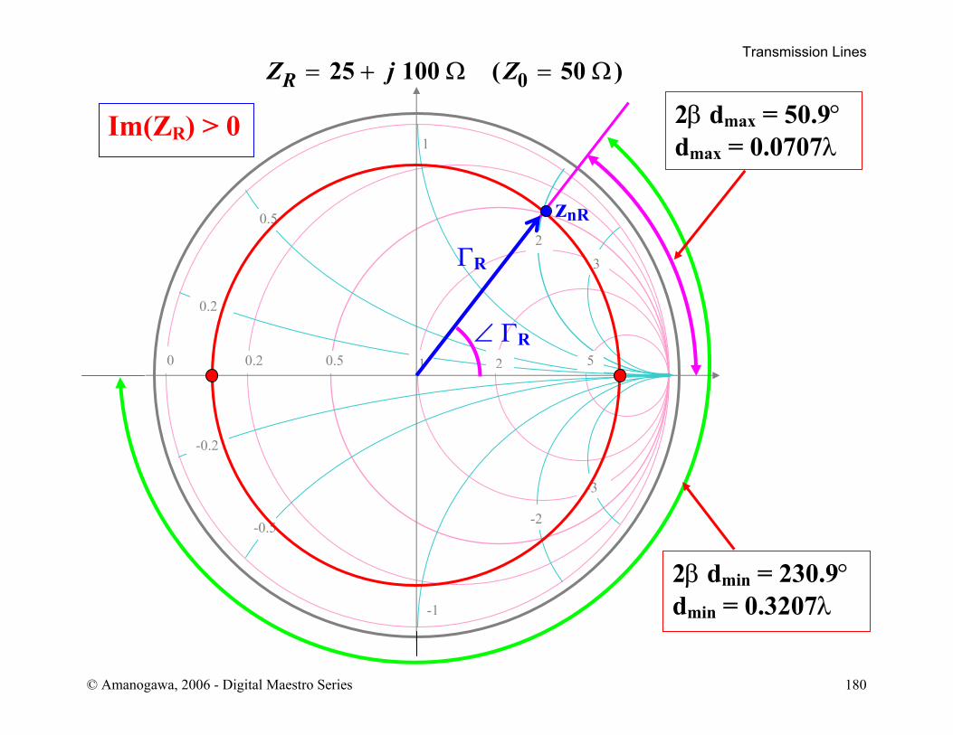
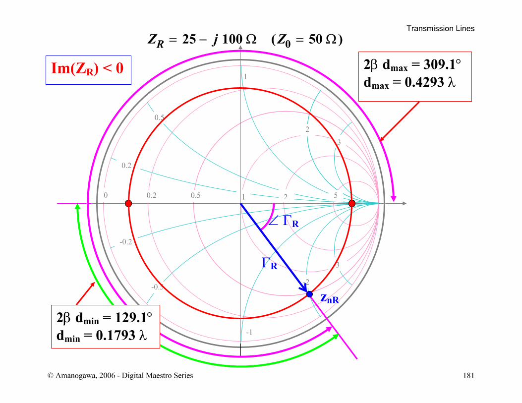
Given ΓR and ZR ⇒ Find dmax and dmin

1. Identify on the Smith chart the load reflection coefficient ΓR or the normalized load impedance ZR .

2. Draw the circle of constant reflection coefficient amplitude |Γ(d)| =|ΓR|. The circle intersects the real axis of the reflection coefficient at two points which identify dmax (when Γ(d) = Real positive) and dmin (when Γ(d) = Real negative)

3. A commercial Smith chart provides an outer graduation where the distances normalized to the wavelength can be read directly. The angles, between the vector ΓR and the real axis, also provide a way to compute dmax and dmin .

Example: Find dmax and dmin for

025 100 ; 25 100 ( 50 )R RZ j Z j Z= + Ω = − Ω = Ω

Transmission Lines


1

-1

0 0.2 0.5 5

0.2

-0.2

21

-0.5

0.5

-3

32

-2

ΓR

znR

∠ ΓR

2β dmin = 230.9° dmin = 0.3207λ

2β dmax = 50.9° dmax = 0.0707λ

Im(ZR) > 0

Z j ZR = + =25 100 500Ω Ω ( )

Transmission Lines


1

-1

0 0.2 0.5 5

0.2

-0.2

21

-0.5

0.5

-3

32

-2

ΓR

znR

∠ ΓR

2β dmin = 129.1° dmin = 0.1793 λ

2β dmax = 309.1°dmax = 0.4293 λ

Im(ZR) < 0

Z j ZR = − =25 100 500Ω Ω ( )

Transmission Lines


Given ΓR and ZR ⇒ Find the Voltage Standing Wave Ratio (VSWR) The Voltage standing Wave Ratio or VSWR is defined as

maxmin

11

R

R

VVSWRV

+ Γ= =

− Γ

The normalized impedance at a maximum location of the standing wave pattern is given by

( ) ( )( )

maxmax

max

1 1!!!

1 1R

nR

dz d VSWR

d+ Γ + Γ

= = =− Γ − Γ

This quantity is always real and ≥ 1. The VSWR is simply obtained on the Smith chart, by reading the value of the (real) normalized impedance, at the location dmax where Γ is real and positive.

Transmission Lines


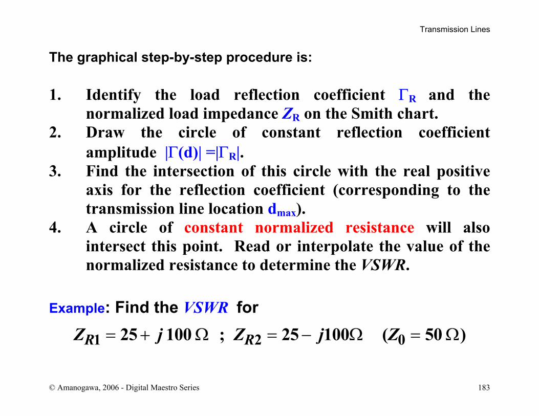
The graphical step-by-step procedure is: 1. Identify the load reflection coefficient ΓR and the

normalized load impedance ZR on the Smith chart. 2. Draw the circle of constant reflection coefficient

amplitude |Γ(d)| =|ΓR|. 3. Find the intersection of this circle with the real positive

axis for the reflection coefficient (corresponding to the transmission line location dmax).

4. A circle of constant normalized resistance will also intersect this point. Read or interpolate the value of the normalized resistance to determine the VSWR.

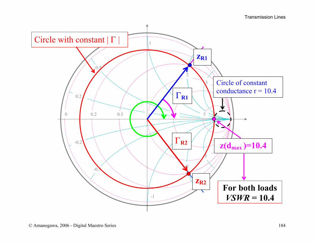
Example: Find the VSWR for

1 2 025 100 ; 25 100 ( 50 )R RZ j Z j Z= + Ω = − Ω = Ω

Transmission Lines


1

-1

0 0.2 0.5 5

0.2

-0.2

21

-0.5

0.5

-3

32

-2

ΓR1

zR1

zR2

ΓR2


z(dmax )=10.4

For both loadsVSWR = 10.4

Circle of constant conductance r = 10.4

Transmission Lines


Given Z(d) ⇐⇒ Find Y(d) Note: The normalized impedance and admittance are defined as

( )( )

( )( )

1 1( ) ( )1 1n n

d dz d y dd d

+ Γ − Γ= =

− Γ + Γ

Since

( )

( )( )

( )

4

1 144 11

4

n n

d d

d dz d y ddd

λ Γ + = −Γ

λ + Γ + − Γλ ⇒ + = = = λ + Γ − Γ +

Transmission Lines


Keep in mind that the equality

( )4n nz d y dλ + =

is only valid for normalized impedance and admittance. The actual values are given by

0

00

4 4( )( ) ( )

n

nn

Z d Z z d

y dY d Y y dZ

λ λ + = ⋅ +

= ⋅ =

where Y0=1 /Z0 is the characteristic admittance of the transmission line. The graphical step-by-step procedure is:

Transmission Lines


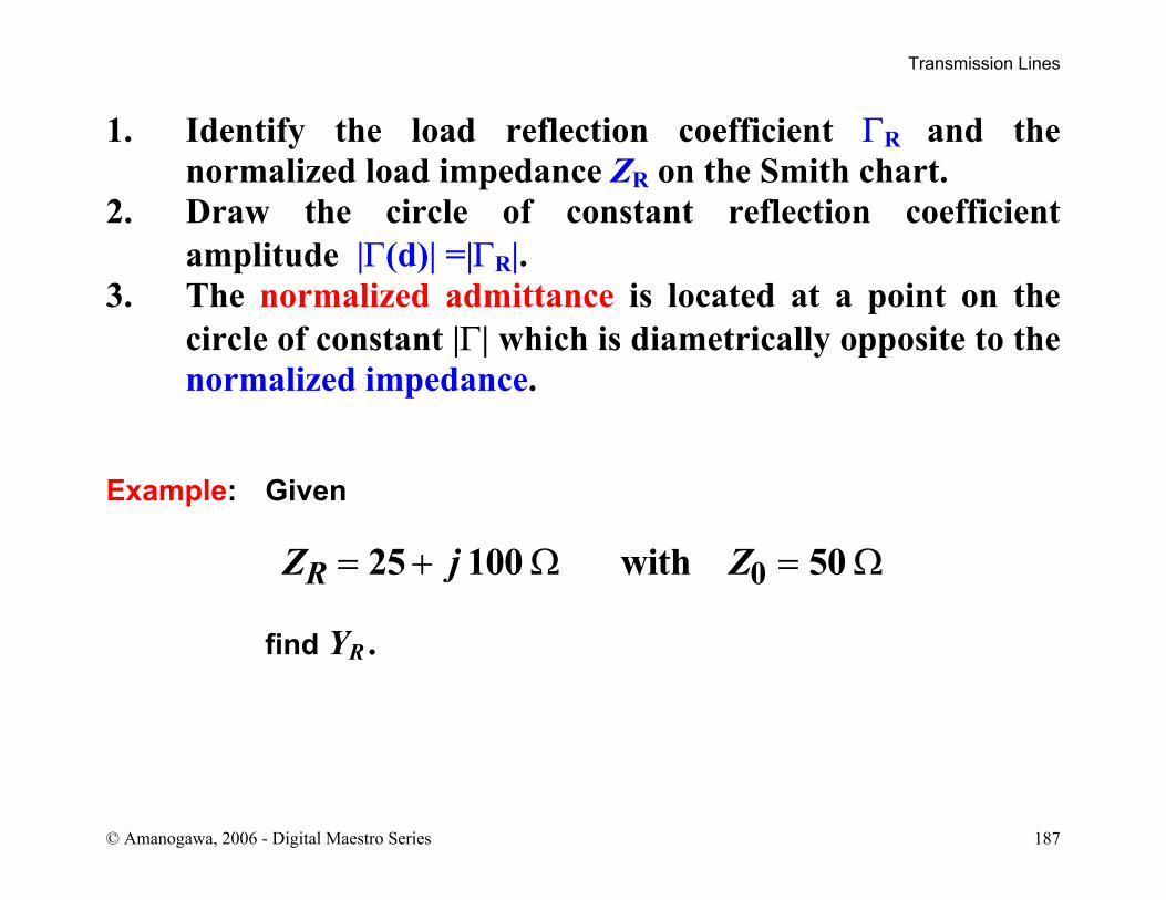
1. Identify the load reflection coefficient ΓR and the normalized load impedance ZR on the Smith chart.

2. Draw the circle of constant reflection coefficient amplitude |Γ(d)| =|ΓR|.

3. The normalized admittance is located at a point on the circle of constant |Γ| which is diametrically opposite to the normalized impedance.

Example: Given

025 100 with 50RZ j Z= + Ω = Ω

find YR .

Transmission Lines


1

-1

0 0.2 0.5 5

0.2

-0.2

21

-0.5

0.5

-3

32

-2

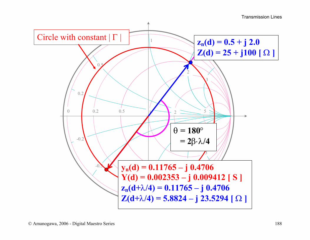
zn(d) = 0.5 + j 2.0 Z(d) = 25 + j100 [ Ω ]

yn(d) = 0.11765 – j 0.4706 Y(d) = 0.002353 – j 0.009412 [ S ] zn(d+λ/4) = 0.11765 – j 0.4706 Z(d+λ/4) = 5.8824 – j 23.5294 [ Ω ]


θ = 180° = 2β⋅λ/4

Transmission Lines


The Smith chart can be used for line admittances, by shifting the space reference to the admittance location. After that, one can move on the chart just reading the numerical values as representing admittances. Let’s review the impedance-admittance terminology:

Impedance = Resistance + j Reactance

Z R jX= +

Admittance = Conductance + j Susceptance Y G jB= +

On the impedance chart, the correct reflection coefficient is always represented by the vector corresponding to the normalized impedance. Charts specifically prepared for admittances are modified to give the correct reflection coefficient in correspondence of admittance.

Transmission Lines


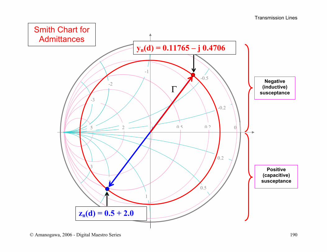
Smith Chart for Admittances

00.20.55

-0.2

0.2

2 1

0.5

-0.5

3

-3

-2

2

-1

1

Positive (capacitive) susceptance

Negative (inductive)

susceptanceΓ

yn(d) = 0.11765 – j 0.4706

zn(d) = 0.5 + 2.0

Transmission Lines


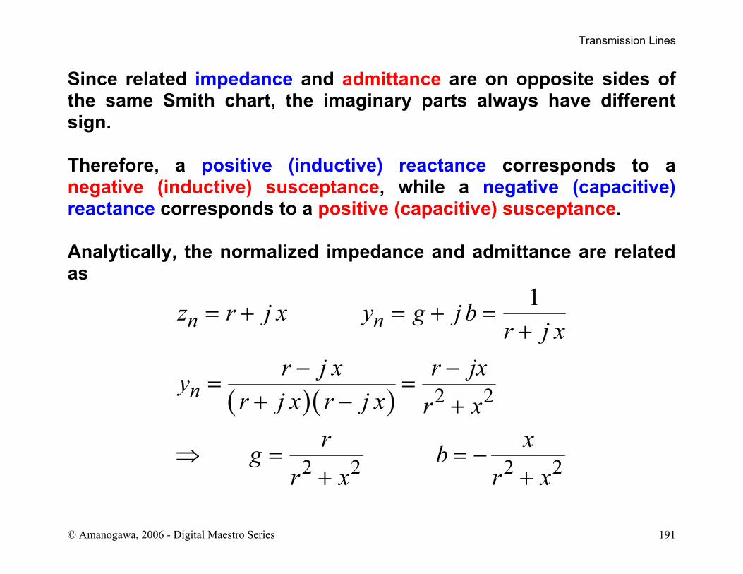
Since related impedance and admittance are on opposite sides of the same Smith chart, the imaginary parts always have different sign. Therefore, a positive (inductive) reactance corresponds to a negative (inductive) susceptance, while a negative (capacitive) reactance corresponds to a positive (capacitive) susceptance. Analytically, the normalized impedance and admittance are related as

( )( ) 2 2

2 2 2 2

1n n

n

z r j x y g jbr j x

r j x r jxyr j x r j x r x

r xg br x r x

= + = + =+

− −= =

+ − +

⇒ = = −+ +

Smith Chart - Amanogawaamanogawa.com/archive/docs/G-tutorial.pdf · Smith Chart The Smith chart is...

Documents

Transcript of Smith Chart - Amanogawaamanogawa.com/archive/docs/G-tutorial.pdf · Smith Chart The Smith chart is...