1

Please note that this is an author-produced PDF of an article accepted for publication following peer review. The definitive publisher-authenticated version is available on the publisher Web site.

Marine Biology January 2015, Volume 162 Issue 1 Pages 15-37 http://dx.doi.org/10.1007/s00227-014-2577-5 http://archimer.ifremer.fr/doc/00247/35859/ © Springer-Verlag Berlin Heidelberg 2014

Achimer http://archimer.ifremer.fr

Small pelagic fish feeding patterns in relation to food resource variability: an isotopic investigation for Sardina

pilchardus and Engraulis encrasicolus from the Bay of Biscay (north-east Atlantic)

Chouvelon Tiphaine 1, 2, *, Violamer L. 1, Dessier Aurelie 1, Bustamante Paco 1, Mornet Francoise 3, Pignon-Mussaud Cecilia 1, Dupuy Christine 1

1 Université de La Rochelle, Littoral Environnement et Sociétés (LIENSs), UMR 7266, CNRS, 2 rue Olympe de Gouges, 17000, La Rochelle 01, France 2 IFREMER, Unité Biogéochimie et Écotoxicologie (BE), Laboratoire de Biogéochimie des Contaminants Métalliques (LBCM), Rue de l’Ile d’Yeu, 44311, Nantes 03, France 3 IFREMER, Unité Halieutique Gascogne Sud (HGS), Station de La Rochelle, Place Gaby Coll, 17087, L’Houmeau, France

* Corresponding author : Tiphaine Chouvelon, email address : tiphaine.chouvelon@hotmail.fr

Abstract : Small pelagic fish represent an essential link between lower and upper trophic levels in marine pelagic ecosystems and often support important fisheries. In the Bay of Biscay in the north-east Atlantic, no obvious controlling factors have yet been described that explain observed fluctuations in European sardine Sardina pilchardus and European anchovy Engraulis encrasicolus stocks, in contrast to other systems. The aim of this study was therefore to investigate to which extent these fluctuations could be trophodynamically mediated. The trophic ecology of both fish species was characterised over three contrasting periods (spring 2010 and 2011 and autumn 2011) in the area, in relation to potential variation in the abundance and composition of the mesozooplankton resource. Stable isotope analyses of carbon (δ13C) and nitrogen (δ15N) were performed on potential mesozoplanktonic prey items and in the muscle of adult fish, as well as in the liver whenever available, and mixing models were applied. In both springs, the mesozooplankton resource was abundant but qualitatively different. During this period of the year, results based on muscle isotope values in particular showed that S. pilchardus and E. encrasicolus likely do not compete strongly for food. On the medium term, E. encrasicolus always presented a greater trophic plasticity than S. pilchardus, both in terms of feeding areas and in the size of the mesozooplanktonic prey consumed. In autumn, mesozooplankton abundances were lower, and it was likely that S. pilchardus and E. encrasicolus share food resources during this period. No clear links between the variation in the mesozooplanktonic resource and the trophic segregation maintained between adults of both fish species in spring could be made. Although a certain potential exists for trophodynamically mediated fluctuations of both species under specific abiotic conditions (i.e. due to the existing trophic segregation in spring in particular), the overall results suggest that fluctuations in abundance of both fish species are probably not directly linked to their trophic ecology in the Bay of Biscay, at least at the level of adult individuals.

Introduction 48

Forage fish such as sardines and anchovies have a key role in marine pelagic ecosystems, representing 49

the main pathway by which energy and nutrients are transported from lower (i.e., plankton) to upper 50

trophic levels (i.e., marine mammals, large fish and seabirds) (Cury et al. 2000). However, the stocks 51

of these small pelagic fish can be highly variable over time (e.g., Schwartzlose et al. 1999). These 52

fluctuations can lead to considerable changes in the structure and function of marine ecosystems, and 53

in turn impact fisheries (FAO 2012). Understanding the processes involved in the fluctuations of 54

forage fish abundance therefore appears critical to maintain marine ecosystem services. 55

For many years, in several marine ecosystems and notably those subjected to upwelling events 56

where sardines and anchovies cohabit (e.g., Benguela Current Ecosystem on the South African coast 57

or Humboldt Current Ecosystem on the Peruvian coast), alternative abundance fluctuations in the 58

populations of both species have been reported (e.g., Lluch-Belda et al. 1989; Barange et al. 2009). 59

Several hypotheses have been proposed to explain these sardine-anchovy fluctuations. Some of these 60

hypotheses rely on the effects of physical, atmospheric and oceanographic regime such as climatic 61

oscillations that potentially control the survival and/or recruitment of one of the other species (e.g., 62

Lluch-Belda et al. 1992; Chavez et al. 2003; Alheit et al. 2012). Takasuka et al. (2007) also proposed 63

that both species display differential “optimal growth temperatures”, so that different climatic 64

conditions can favour one species or the other during early life stages. This hypothesis extends the 65

“optimal environmental window” theory of Cury and Roy (1989), establishing the conditions for the 66

recruitment success of pelagic fish in upwelling areas. Other hypotheses proposed for explaining 67

sardine-anchovy alternations include biological controlling factors such as intra-guild predation (e.g., 68

Irigoien and De Roos 2011), or trophodynamically mediated fluctuations with the resource’s 69

variability favouring one species or the other (e.g., Van der Lingen et al. 2006). Some studies that have 70

investigated the diet of both species simultaneously (e.g., Louw et al. 1998; Van der Lingen et al. 71

2006; Espinoza et al. 2009) have effectively demonstrated that sardines and anchovies (generally adult 72

individuals) show distinct feeding strategies, especially in terms of the size of copepod they 73

preferentially consume. Hence, warmer or cooler oceanographic regimes would favour the 74

development of small or larger planktonic prey species, and thus one or other small pelagic predator. 75

Simply determining the effects of abiotic factors influencing both the recruitment and survival of early 76

life stages is thus not sufficient to understand fluctuations in the abundance of small pelagic fish. The 77

knowledge of trophic interactions between species as well as fluctuations in food resource and their 78

impact on trophic interactions also appears a crucial step. 79

Stable isotope analysis (SIA) of carbon (!13C) and nitrogen (!15N) of the tissues of consumers 80

and their putative prey has proven to be a powerful tool to describe the trophic ecology of marine 81

organisms, representing an alternative or complementary tool to the traditional methods of dietary 82

studies such as the analysis of stomach contents (Michener and Kaufman 2007). Primary producers of 83

an ecosystem generally display different isotopic compositions (Peterson and Fry 1987; France 1995) 84

and the enrichment in 13C and 15N between a source and its consumer (also called Trophic Enrichment 85

Factor, TEF) is relatively predictable. This enrichment is less important in 13C (" 1‰) than in 15N 86

(3.4‰ on average) (De Niro and Epstein 1978, 1981; Post 2002). Hence, !13C values are generally 87

considered as a conservative tracer of the primary producer at the base of the food web supporting 88

consumers, and consequently a tracer of their foraging habitat (France 1995; Hobson 1999). 89

Alternatively, !15N values are generally used as a proxy of their trophic position (Vander Zanden et al. 90

1997; Post 2002). Furthermore, for some years, mixing models integrating !13C and !15N values of 91

prey and predators have proved their utility to decipher the contribution of different prey items in the 92

diet of a predator (Parnell et al. 2010, 2013; Phillips et al. 2014). This may be particularly useful when 93

studying the trophic links between plankton and small pelagic planktivorous fish (e.g., Costalago et al. 94

2012), because of the peculiar difficulty in observing direct interactions between these organisms in 95

the open water environment, and because the small size of plankton can make stomach content 96

analysis particularly difficult. Moreover, isotope values provide information on the food assimilated at 97

a time scale that depends on the turnover of the tissue analysed (Tieszen et al. 1983; Hobson and Clark 98

1992; Sponheimer et al. 2006). For instance, carbon and nitrogen half-lives in fish tissues were shown 99

to vary from 5-14 days in the liver to 19-21 days in the muscle of the juvenile Japanese bass 100

Lateolabrax japonicus (Suzuki et al. 2005), from 3-9 days in the liver to 25-28 days in the muscle of 101

the juvenile sand goby Pomatoschistus minutus (Guelinckx et al. 2007), and from 10-20 days in the 102

liver to 49-107 days in the muscle of the flat fish Paralichthys dentatus (Buchheister and Latour 103

2010). 104

The Bay of Biscay is a very large bay located in the north-east Atlantic Ocean. It supports a 105

rich fauna including many protected species, e.g., marine mammals, seabirds, sharks and rays, and is 106

subjected to numerous anthropogenic activities including important fisheries (Lorance et al. 2009; 107

OSPAR 2010). In particular, European sardine (Sardina pilchardus) and European anchovy 108

(Engraulis encrasicolus) fisheries are of major importance in the area (ICES 2010a). No quota 109

currently exists for sardine despite an observed decrease in their catches in this area (OSPAR 2010). 110

Conversely, a decrease in anchovy stocks during the 2000s led to the closing of its fishery in 2005. 111

The moratorium ended in 2010 and finally resulted in the establishment of quotas for this species 112

(ICES 2010a, b). In the Bay of Biscay, strong fluctuations in the abundance of small pelagic fish such 113

as sardines and anchovies have been observed for several years (ICES 2010a). However, in contrast to 114

upwelling areas where alternative abundance fluctuations have been demonstrated and/or linked to 115

climatic events or biological controlling factors (see above), no clear relationships between both fish 116

species have yet been shown in the Bay of Biscay ecosystem. Sardine and anchovy have always 117

demonstrated both alternation and co-occurrence in spring-survey data (ICES 2010b) and no obvious 118

controlling factors have been identified to-date explaining general fluctuations in the abundances of 119

small pelagic fish in the area. Besides, an ecological network analysis of the Bay of Biscay continental 120

food web provided evidence that bottom-up processes play a significant role in the population 121

dynamics of upper-trophic levels and in the global structuring of this marine ecosystem (Lassalle et al. 122

2011). 123

In a previous study in the area, Chouvelon et al (2014) examined the trophic ecology of adults 124

of the two fish species by SIA during a single specific period (spring 2010). The authors highlighted a 125

trophic segregation between species during the study period. This may support the hypothesis that 126

fluctuations of both fish species’ abundances could be, at least in part, trophodynamically mediated, if 127

the food environment on the medium to long-term would tend to favour one species or the other, as a 128

function of their respective dietary preferences (Van der Lingen et al. 2006). However, no link could 129

be made with food resource composition and availability in this previous study (Chouvelon et al. 130

2014), because only one period of sampling and a single tissue (muscle tissue, i.e., medium to long-131

term integrator of the food assimilated) were considered. Demonstration of such a link could highlight 132

a strong dependency of one or both fish species to resource composition and availability, and/or reveal 133

a relative trophic plasticity in one or both species relative to food resource variability. This may finally 134

help to understand to which extent fluctuations and/or alternations of both species may be strongly 135

trophodynamically mediated or not in the area. 136

In this general context, the aim of this study was twofold: 1) investigating intra- (seasonal) and 137

inter-annual variations in the trophic ecology of adult sardines and anchovies from the Bay of Biscay; 138

2) linking potential temporal variation in the diet of both fish species with variations in the 139

mesozooplankton resource, to depict potential differential feeding strategies in both fish species in 140

relation to resource variability. Several studies have highlighted that zooplankton (and notably 141

copepods belonging to the mesozooplankton community) are by far the most important dietary 142

component for sardines and anchovies compared to phytoplankton (e.g., Van der Lingen et al. 2006; 143

Espinoza et al. 2009; Nikolioudakis et al. 2012;). As such, we focused on mesozooplanktonic prey as 144

the major food resource for both fish species in the present study. Three different periods of sampling 145

with contrasting abiotic conditions were considered, with one of these periods referring to those 146

investigated by Chouvelon et al. (2014). SIA was undertaken on identified mesozooplanktonic prey 147

and predators and mixing models used to estimate consumption patterns. The results obtained provide 148

some understanding as to what extent potential trophodynamic differences and/or dependence on food 149

resource variability (composition and availability) can influence fluctuations and/or alternations of 150

both fish species abundances in the highly productive Bay of Biscay area. 151

152

Materials and Methods 153

154

Sample collection 155

156

Mesozooplankton and fish samples were collected in the spring of 2010 and 2011 and autumn of 2011, 157

during sea surveys conducted by the French Research Institute for the Exploitation of the Sea 158

(IFREMER) on the continental shelf to the shelf-edge of the Bay of Biscay: PELGAS 2010 and 159

PELGAS 2011 surveys (25th April – 5th June 2010 and 26th April – 4th June 2011, respectively), and 160

EVHOE 2011 survey (18th October – 30th November 2011). As noted above, isotope values of samples 161

from the PELGAS 2010 survey were presented in a previous study in the area (Chouvelon et al., 162

2014), as well as the methodological aspects related to the study of trophic relationships between 163

mesozooplankton and planktivorous fish through SIA. Isotope results of the spring 2010 survey are 164

thus only used here for direct comparison with the two other periods examined (i.e., spring and 165

autumn 2011), and further links with the variation in resource abundance between the three periods. 166

These seasons were selected for sampling for various reasons regarding the objectives of the 167

study. First, it was hypothesized that food resource abundance and composition would greatly differ 168

between spring and autumn, i.e., between seasons presenting different environmental conditions in 169

temperate areas such as the Bay of Biscay (Villate et al. 1997; Valdés and Moral 1998, Zarauz et al. 170

2007). Moreover, survey data indicated that both springtime periods were different in terms of 171

temperature and salinity patterns in particular, potentially leading to different food resource 172

availability as well (i.e., warmer sea surface temperatures during the spring 2011 campaign, in 173

comparison with the spring 2010 campaign; IFREMER survey data, see also 174

www.previmer.org/observations). Finally, sampling seasons were chosen with regard to the main 175

spawning period of both fish species, potentially driving different feeding strategies in the study 176

fishes. Indeed, for the Bay of Biscay anchovy, the peak spawning period has been reported to be in 177

spring (i.e., May-June; Motos 1996), and the onset of spawning is concurrent with the sharp seasonal 178

increase in surface temperature (ICES 2010b). Even though feeding migrations would occur after 179

spawning (i.e., in summer and autumn), with fat content increasing during these seasons (Dubreuil and 180

Petitgas 2009), anchovy continue to feed during the spawning season (Plounevez and Champalbert 181

1999), with the duration of the spawning season depending on energy intake during this period (ICES, 182

2010b). For the Atlanto-Iberian and Biscay sardine, the main spawning period is between October and 183

June and thus partly overlaps with those of anchovy in the Bay of Biscay (ICES 2010b). As for 184

anchovy, fat content peaks in early autumn (i.e., beginning of the spawning season), although sardines 185

also feed throughout the year (ICES 2010b). 186

Mesozooplankton were collected by vertical trawls of 200#m mesh-size WP2 nets, from 100m 187

depth (or bottom depth for inshore stations) to the surface. 10 to 16 stations were selected depending 188

on the survey (Fig. 1). During PELGAS (spring) surveys, the stations followed transects used for the 189

hydroacoustic assessment of small pelagic fish biomass. They were thus distributed from the north to 190

the south of the Bay of Biscay, and from the coastline (C) to the continental slope (Sl) including 191

stations over the continental shelf (Sh) (Fig. 1A). During PELGAS 2011, one oceanic (O) station was 192

also considered (Fig. 1B). During EVHOE 2011 survey, stations followed randomly distributed 193

fishing trawls, although as in PELGAS the stations were selected in order to cover all the Bay of 194

Biscay area (Fig. 1C). After collection, mesozooplankton samples were concentrated on a 200#m 195

mesh and preserved in 70% ethanol for further taxonomic identification and stable isotope analysis. 196

Adult sardines and anchovies were collected by pelagic trawls during PELGAS surveys (76*70 197

trawl with vertical opening of ~ 25 m, or 57*52 trawl with vertical opening 15-20 m), and by bottom 198

trawls during EVHOE survey (large vertical opening (GOV) trawl 36/47). This is due to a difference 199

in the main initial objectives of the surveys (i.e., assessing abundance and distribution of pelagic fish 200

in the Bay of Biscay using acoustic method during PELGAS; assessing abundance and distribution of 201

demersal and benthic resources using bottom trawl during EVHOE). During each survey and for each 202

fish species, individuals were collected in 7 to 8 trawls over the continental shelf (Fig. 1). In some 203

trawls, both species occurred at the same time however this does not indicate that they come from the 204

same shoal given the duration of each trawl (between 30 to 60 minutes). Fish were immediately frozen 205

at -20°C until further dissection and analyses back to the laboratory. 206

207

Taxonomic determination of mesozooplankton and preparation for analysis 208

209

Taxonomic identification of mesozooplankton was carried out at the laboratory with a Leica M3Z 210

stereo microscope (mag. x65 to x160), to genus and to species level whenever possible. For each 211

spring station, identified taxa contributing at least 5% of the total abundance of the sample both in 212

number (individuals. m-3) and in biomass (mg. m-3) (i.e., ‘dominant taxa’), and likely to be part of the 213

diet of sardines and anchovies (i.e., species that may be found in stomach contents of anchovies from 214

the Bay of Biscay area as reported by Plounevez and Champalbert (1999)) were sorted for further SIA. 215

For each autumn station, as the diversity was lower, only identified taxa contributing at least to 10% of 216

the total abundance of the sample both in number and in biomass were subsequently sorted for SIA. 217

As such, one to four ‘dominant taxa’ were analysed for stable isotope ratios within each of the stations 218

sampled over the three periods. Details for the calculation of the relative abundance of each identified 219

taxa in number and in biomass can be found in Chouvelon et al. (2014). 220

Depending on their size, 20 to 350 individuals belonging to each of the ‘dominant taxa’ were 221

taken out from ethanol and carefully washed with distilled water in order to completely remove the 222

ethanol, detritus and phytoplankton. Sorted and washed organisms were finally frozen at -80°C for 48h 223

to be freeze-dried (24h). A pool of individuals for each species sorted by station was then packed into 224

2 tin capsules for stable isotope analysis (i.e., half of sorted organisms within each capsule) and the 225

mean value of the two capsules was used in further data analyses (Chouvelon et al. 2014). 226

For each fish species and for each survey, 30 to 40 adult individuals of similar size classes 227

(average total length ± standard deviation (SD) of 18.1 ± 2.2 cm and 13.9 ± 1.6 cm for sardines and 228

anchovies, respectively) were defrosted and dissected at the laboratory to obtain portions of dorsal 229

white muscle as well as the liver (Pinnegar and Polunin 1999). Specifically, the average total length 230

for sardines was of 17.3 ± 2.6 cm, 18.7 ± 0.7 cm and 18.4 ± 2.6 cm for individuals collected in spring 231

2010, spring 2011 and autumn 2011, respectively. The average total length for anchovies was of 14.6 232

± 1.8 cm, 13.3 ± 1.1 cm and 13.7 ± 1.5 cm for individuals collected in spring 2010, spring 2011 and 233

autumn 2011, respectively. Within each species and at each season, these sizes corresponded to mature 234

individuals and allowed comparison of morphologically similar fishes (i.e., adult individuals) at the 235

three seasons investigated. Also, sardines were larger than anchovies, because the size at maturity is 236

higher for sardines (i.e., about 14 cm length, 1 to 2 years old individuals) than for anchovies (i.e., 237

about 10 cm length, one year old) (ICES 2010b). Muscle and liver samples were individually stored 238

frozen at -20°C in plastic bags prior to a 72h freeze-drying period. White muscle and liver samples 239

were ground manually or with a planetary ball mill (Retsch PM 200), and were treated with 240

cyclohexane in order to remove naturally 13C-depleted lipids (De Niro and Epstein 1977). Lipid-free 241

samples were finally dried in an oven at 45°C for 48h and packed in tin capsules for SIA. 242

243

Stable isotope analysis 244

245

The natural abundance of carbon and nitrogen stable isotopes in plankton and fish was determined 246

with a Thermo Scientific Delta V Advantage mass spectrometer coupled to a Thermo Scientific Flash 247

EA1112 elemental analyser. Results are expressed as isotope ratios !X (‰) relative to international 248

standards (Pee Dee Belemnite for carbon and atmospheric N2 for nitrogen), according to the formula: 249

!X = [ (Rsample / Rstandard) – 1] x 103 250

where X = 13C or 15N and R = 13C/12C or 15N/14N (Peterson and Fry 1987). Replicate measurements of 251

internal laboratory standards (acetanilide) indicated a precision of 0.2‰ for both !13C and !15N values. 252

253

Data treatment and statistical analyses 254

255

Chouvelon et al. (2014) demonstrated a significant effect of preservation (ethanol 70% vs. freezing at -256

20°C) and of lipid content on mesozooplankton !13C and !15N values. In the present study, for 257

consistency of the treatment applied to prey and predators both in terms of preservation and of lipid 258

correction, we thus applied the same corrections as proposed by Chouvelon et al. (2014) for further 259

analysis of the diet of sardine and anchovy through SIA. Briefly, this consisted in correcting !13C and 260

!15N values of all mesozooplanktonic organisms preserved in 70% ethanol for the effect of ethanol, 261

and only !13C values of mesozooplanktonic organisms were corrected for the effect of lipid content 262

(Chouvelon et al. 2014). The corrected values were then used in further statistical analyses and mixing 263

models. 264

All statistical analyses were conducted with R (R Development Team 2011). Normality of all 265

data was tested using Shapiro-Wilk’s tests, i.e., for further use of parametric or non-parametric 266

statistics. A Student t test or a Mann-Whitney-Wilcoxon test was thus applied when comparing two 267

series of samples, e.g., for testing significant difference between both species. Similarly, an ANOVA 268

(followed by post-hoc Tukey tests) or a Kruskal-Wallis test (followed by a multiple comparison test 269

with Holm’s adjustment method) was applied when comparing more than two series of samples, e.g., 270

for testing significant difference between periods. 271

In order to link potential variations in the trophic ecology of both fish species inferred from 272

SIA with the variability of the mesozooplankton resource, data on mesozooplankton abundances 273

presented in the present study mainly concerns the taxa contributing to more than 5% of the total 274

abundance both in number and in biomass, in at least one station for one of the periods considered 275

(‘dominant taxa’). These taxa were effectively those analysed for SIA and considered in mixing 276

models (see following section). The representativeness of these ‘dominant taxa’ relative to the whole 277

mesozooplankton community was previously checked by analysing the correlation between total 278

mesozooplankton abundance and total abundance of these ‘dominant taxa’ through a Spearman 279

correlation coefficient test. 280

281

Isotopic mixing models 282

283

To account for numerous potential prey items in the diets of sardines and anchovies, the wide 284

variability in the !13C and !15N values of mesozooplancton, and for the uncertainty of TEFs (i.e., the 285

difference ($) in !13C and !15N between the predator’s tissue analysed and its diet), Bayesian isotopic 286

mixing models were used (available as an open source R package SIAR; Parnell et al. 2010). In 287

mixing models that are mathematically underdetermined (with more unknowns than equations and no 288

unique solution) where the number of sources exceeds n+1 (Phillips and Gregg 2003), one possible 289

approach to encompass this common problem and to simplify the analysis is to combine some sources 290

(Phillips et al. 2005). In the present study, potential prey items, that is all entities ‘taxa-station’ 291

(e.g., ‘Temora sp.-C2’, ‘Medium undetermined Calanoid-Sh3’) analysed for isotopes were thus 292

grouped before running SIAR. As in Chouvelon et al. (2014), this grouping was performed through a 293

Hierarchical Cluster Analysis (HCA) for each period considered. HCA were based on !13C and !15N 294

values, average size (total length) of organisms (see Table 1), and geographical coordinates of each 295

entity ‘taxa-station’ analysed for isotope ratios. The groups defined by HCA were then used in mixing 296

modelling (Table 2). 297

To the best of our knowledge, precise TEFs are still unknown for mesozooplankton-feeders 298

such as sardines and anchovies. Post (2002) suggested that TEFs of 0.4 ± 1.3‰ and 3.4 ± 1‰ for !13C 299

and !15N, respectively, could be widely applicable within a food web. Nevertheless, there is increasing 300

evidence in the literature that TEFs may be highly variable as a function of the consumer’s taxa, or as 301

a function of the type and the quality of the consumer’s food (e.g., Vanderklift and Ponsard 2003; Caut 302

et al. 2009). Recent studies have also shown that even considering uncertainty around TEFs or 303

discrimination factors, Bayesian models outputs may be very sensitive to the chosen TEFs (e.g., Bond 304

and Diamond 2011). To apply sensitivity analyses on the results obtained, four mixing models by 305

species and by tissue were thus run using different values of TEFs found in the literature, for both !13C 306

and !15N (Post 2002, for general values; Pinnegar and Polunin 1999; Trueman et al. 2005; and 307

Sweeting et al. 2007a, b for fish muscle or liver in particular; see Table 4 for the detailed TEFs used). 308

The variability around !13C and !15N values of each source taken into account in the mixing models 309

corresponded to the standard deviation around the mean of each source group (i.e., SD given in Table 310

2). For each period considered, for each tissue and for each species, an average value of the estimated 311

contribution of each group of mesozooplankonic prey was finally calculated from the four mixing 312

models applied (Table 4). 313

314

Results 315

316

General abundance and distribution patterns in the mesozooplankton community 317

318

Over the three study periods and considering all the stations selected for taxonomical identification, 319

total abundance of mesozooplankton (in number) was the highest in spring 2010 and varied between 320

541 to 7417 ind. m-3 (mean ± SD: 3316 ± 2609 ind. m-3, CV = 79% for the 13 stations covered at this 321

period in the Bay of Biscay area). In spring 2011, total abundances were slightly lower on average but 322

varied among a similar range of values, i.e., from 305 to 8433 ind. m-3 (1935 ± 2108 ind. m-3, CV = 323

109% for the 16 stations covered). Total abundances finally displayed the lowest values in autumn 324

2011, varying from 53 to 3366 ind. m-3 (758 ± 1042 ind. m-3, CV = 138% for the 10 stations covered). 325

Within the whole mesozooplankton community, the percentage of copepods relative to the total 326

abundance of mesozooplanktonic organisms varied from 21 to 99% in spring 2010, and from 49 to 327

96% in spring 2011. The values were the highest in autumn 2011, varying from 72 to 97% (Fig. 2). 328

The correlation between the total abundance of mesozooplankton (in number) and the 329

abundance of taxa contributing to more than 5% of the total abundance (i.e., ‘dominant taxa’) was 330

highly significant (rSpearman = 0.984, p < 0.0001, n = 39 stations – i.e., all stations covered during the 331

three periods investigated). This indicated these ‘dominant taxa’ of the wider mesozooplankton 332

community. In spring of 2010 and 2011, coastal stations were mainly characterised by small to 333

medium-sized organisms such as Acartia sp., Temora sp. or Appendicularia (Fig. 3A). The large 334

copepod C. helgolandicus (especially abundant in spring 2010) or the smaller Oithona sp. were more 335

abundant in stations from the shelf and/or from the slope, or in the station O4 from the oceanic area 336

sampled in spring 2011. In autumn 2011, the copepods Oncaea sp. and Temora sp. were the most 337

abundant in stations located near the coast and/or on the shelf, while large Decapod larvae were 338

abundant in 2 out of the 10 stations analysed. Total abundances in stations located on or near the slope 339

were very low at this period (Fig. 3). 340

Finally, the proportion of small organisms (see Table 1 for size ranges) was relatively stable 341

throughout the three periods considered, varying between 51 to 55% relative to the whole 342

mesozooplankton community (i.e., community now represented by the ‘dominant taxa’) (Fig. 4A). 343

The proportion of medium-sized organisms was higher in both spring and autumn 2011 (44 and 43%, 344

respectively) than in spring 2010 (34%), whereas the proportion of large organisms such as 345

C. helgolandicus was the highest in spring 2010 (16% vs. 4% and 2% in spring and autumn 2011, 346

respectively) (Fig. 4A). Abundances of organisms were the highest in stations from the coast and from 347

the shelf both in spring and autumn 2011 (Figs. 3 and 4). However in spring 2011, a non-negligible 348

part of the total abundance of mesozooplankton also belonged to stations from the slope (i.e., 21%), as 349

well as in spring 2010 where high abundances of organisms were found in the more oceanic stations 350

(i.e., 32%) (Figs. 3 and 4). 351

352

Definition of prey groups and variability of mesozooplankton "13C and "15N values 353

354

The HCA defined eight, nine and six groups of prey for spring 2010, spring 2011 and autumn 2011, 355

respectively (Table 2). As such, the groups reflected a certain ecological significance for further 356

interpretation of the results of isotopic models, both in terms of sizes of organisms and in terms of 357

their sampling location. Isotope values of the different groups were relatively distinct from each other 358

(Table 2). Average !15N values varied from 4.2 ± 0.6 (group 1) to 7.2 ± 0.9‰ (group 8) in spring 359

2010, from 4.6 ± 0.3 (group 1) to 8.9 ± 0.6‰ (group 6) in spring 2011, and from 2.4 ± 0.2 (group 1) to 360

7.0 ± 0.4‰ (group 4) in autumn 2011. Average !13C values varied from -22.2 ± 0.1 (group 6) to -19.4 361

± 0.3‰ (group 2) in spring 2010, from -21.8 ± 0.4 (group 1) to -19.0 ± 0.6‰ (group 7) in spring 2011, 362

and from -20.9 ± 0.0 (group 4) to -20.2 ± 0.2‰ (group 5) in autumn 2011 (Table 2). Groups with large 363

bodied organisms generally displayed higher !15N values than those containing small to medium-sized 364

organisms within a same area. Also, within a same range of sizes, organisms collected in coastal 365

waters generally displayed higher !15N values than those collected in more oceanic waters (Table 2). 366

For instance, in spring 2010, large organisms from the shelf to the slope in the northern part (group 5) 367

showed an average !15N value of 7.1 ± 0.9‰. On the contrary, the average !15N value of small to 368

medium-sized organisms from the slope in the northern part (group 1) was of 4.2 ± 0.6‰, and in the 369

same area, small to medium-sized organisms from the coast to the shelf in the northern part (group 4) 370

displayed an average !15N value of 7.0 ± 0.6‰. In spring 2011, the same pattern of differences could 371

be observed between these three types of groups collected in the northern part (corresponding to group 372

3, groups 1 and 2 considered together, and group 6, respectively). This was also the case of groups 373

from the southern area. Large organisms from the shelf to the slope (group 7) showed an average !15N 374

value of 7.6 ± 0.7‰, while those of small to medium-sized organisms from shelf to the slope (group 4) 375

was of 5.6 ± 0.5‰. Small to medium-sized organisms from the coast to the shelf (group 8) displayed 376

an average !15N value of 7.2 ± 0.3‰ (Table 2). 377

378

Fish muscle "13C and "15N values and isotopic mixing models 379

380

Within each of the three periods considered, S. pilchardus and E. encrasicolus differed significantly 381

for both muscle !13C and !15N values (all p-values < 0.05; Table 3). E. encrasicolus always had lower 382

!13C and !15N values on average than S. pilchardus (Table 3, Fig. 5). In S. pilchardus, individuals 383

sampled in autumn 2011 displayed significantly lower muscle !13C values than individuals sampled in 384

both spring 2010 and 2011, while !15N values were not significantly different between periods (p-385

values > 0.05, Table 3). In contrast in E. encrasicolus, muscle !13C values were not significantly 386

different between individuals collected at the three periods, but individuals collected in autumn 2011 387

showed significantly higher !15N values than those sampled in springs 2010 and 2011 (Table 3, Fig. 388

5). 389

In spring 2010, 3 groups out of the 8 previously defined mainly contributed to the diet of 390

S. pilchardus, whatever the TEF used: group 8 corresponding to small to medium-sized organisms 391

from the coast to the shelf in the central to southern part (average mean contribution ± SD = 43.7 ± 392

5.9%), group 4 corresponding to small to medium-sized organisms from the coast to the shelf in the 393

northern part (28.9 ± 9.6%), and in lower proportion group 5 corresponding to large organisms from 394

the shelf to the slope in the northern part (14.7 ± 9.5%; Table 4). The same three groups presented the 395

highest estimated contribution in the diet of E. encrasicolus as well (22.3 ± 7.7%, 19.3 ± 7.7% and 396

17.6 ± 10.0% for groups 8, 4 and 5, respectively). However in the latter species, two other groups also 397

contributed significantly to its diet (i.e., average contribution close to or % 10%): namely group 6 398

corresponding to large organisms from the slope in the central to southern part (13.1 ± 11.8%), and 399

group 2 containing medium-sized organisms from the coast to the shelf in the central to northern part 400

(11.3 ± 10.8%; Table 4). 401

In spring 2011, 4 groups out of the 9 defined mainly contributed to the diet of S. pilchardus and 402

E. encrasicolus (i.e., average contribution % 10% in both species): group 6 containing small to 403

medium-sized organisms from the coast in the northern part (40.8 ± 16.0% and 11.2 ± 8.1% in S. 404

pilchardus and E. encrasicolus, respectively), group 3 corresponding to large organisms from the shelf 405

to the slope in the northern part (17.4 ± 13.8% and 29.6 ± 24.8% in S. pilchardus and E. encrasicolus, 406

respectively), group 8 corresponding to small to medium-sized organisms from the coast to the shelf in 407

the southern part (12.4 ± 13.0% and 11.7 ± 14.7% in S. pilchardus and E. encrasicolus, respectively), 408

and finally group 7 including large organisms from the shelf to the slope in the southern part (12.1 ± 409

12.1% and 9.5 ± 9.8% in S. pilchardus and E. encrasicolus, respectively). In total, these four groups 410

(i.e., groups 3, 6, 7 and 8) contributed on average to 82.7% and 62.0% to the diet of S. pilchardus and 411

E. encrasicolus, respectively (Table 4). However, group 6 presented the highest contribution in S. 412

pilchardus (40.8 ± 16.0%) whatever the TEF used, the group 3 was the most significant group in the 413

diet of E. encrasicolus (29.6 ± 24.8%) in 3 out of the 4 models performed (Table 4). 414

Mixing models performed on !13C and !15N values in the muscle of the fish sampled in autumn 415

2011 highlighted the major contribution of 3 of the 6 groups defined in the diet of both species. In 416

total, group 4 (corresponding to small to medium-sized organisms from the coast to the shelf in the 417

northern part) and group 5 (containing small to medium-sized organisms from the coast to the shelf in 418

the central part) both contributed on average 76.5% and 69.7% to the diet of S. pilchardus and 419

E. encrasicolus, respectively (Table 4). Group 6 including small to medium-sized organisms from the 420

coast to the slope in the southern part was the third contributor to the diet of both species, with an 421

average contribution of 12.6 ± 7.2% and 14.0 ± 6.8% in S. pilchardus and E. encrasicolus, 422

respectively (Table 4). 423

424

Fish liver "13C and "15N values and isotopic mixing models 425

426

In both spring and autumn 2011, S. pilchardus and E. encrasicolus differed significantly in liver 427

!13C values (both p-values < 0.05). E. encrasicolus always displayed lower !13C values on average 428

than S. pilchardus (Table 3, Fig. 5). However, liver !15N values did not differ significantly between 429

both species at both periods. In S. pilchardus, individuals sampled in autumn 2011 showed 430

significantly lower !13C values and higher !15N values than those sampled in spring 2011. In E. 431

encrasicolus, individuals collected in autumn 2011 had higher average !15N values than those sampled 432

in spring 2011, but !13C values did not differ between seasons (Table 3, Fig. 5). 433

Interestingly in both species, mixing models performed on liver !13C and !15N values of the fish 434

sampled in spring 2011 showed an average contribution of all the defined prey groups % 5% (Table 4). 435

Four to 5 groups out of the 9 defined presented an average contribution %10% in both species, with 436

group 6 (containing small to medium-sized organisms from the coast in the northern part), group 3 437

(including large organisms from the shelf to the slope in the northern part) and group 9 (corresponding 438

to small to medium-sized organisms from the oceanic area) being common major groups (given here 439

in the increasing order of contribution) for both fish species. Other major groups contributing to their 440

short-term diet were group 4 (including small to medium-sized organisms from the shelf to the slope 441

in the central to southern part) and group 8 (corresponding to small to medium-sized organisms from 442

the coast to the shelf in the northern part) in S. pilchardus, and the group 1 in E. encrasicolus 443

(containing small to medium-sized organisms from the slope in the northern part) (Table 4). 444

In autumn 2011, the results of the mixing models based on liver tissues were quite similar to 445

those obtained with models performed on muscle !13C and !15N values. The same 3 groups out of the 6 446

defined contributed significantly to the diet of both species (i.e., groups 4, 5 and 6). Group 4 447

(corresponding to small to medium-sized organisms from the coast to the shelf in the northern part) 448

contributed more than 50% on average to the diet of both species (53.7 ± 20.6% and 53.0 ± 28.3% in 449

S. pilchardus and E. encrasicolus, respectively; Table 4). Group 2 including small to medium-sized 450

organisms from the slope in the northern part also contributed 10.7 ± 5.3 % on average to the short-451

term diet of E. encrasicolus. 452

453

Discussion 454

455

Spatial, temporal and size-related variability of mesozooplankton abundances and isotope values over 456

time 457

458

With all stations taken into account within a given period, the average total abundances of 459

mesozooplankton showed a general decreasing trend over the three periods considered with spring 460

2010 > spring 2011 > autumn 2011. In all cases, copepods dominated the mesozooplankton 461

community, with the exception of some coastal stations (e.g., C4) that sometimes displayed a 462

relatively high percentage of meroplankton or other taxa (e.g., Appendicularia, Cladocerans), 463

especially in spring. These general patterns in the composition of the mesozooplankton community 464

analysed here are consistent with the current knowledge on this compartment concerning European 465

shelf seas (Williams et al. 1994), and more specifically concerning the Bay of Biscay area (Villate et 466

al. 1997; Valdés and Moral 1998; Plounevez and Champalbert 1999; Albaina and Irigoien 2004). 467

When focusing on abundances and distribution of the ‘dominant taxa’, which were well correlated 468

with total mesozooplankton abundances, the abundances were generally higher in coastal stations and 469

notably in autumn. This is quite common for neritic areas at this latitude: i.e., maximum densities are 470

generally observed in late spring extending into summer, a secondary peak of high biomass occurs in 471

autumn, and values are minimum in winter. In contrast, oceanic areas generally present a single annual 472

peak in spring, there is no autumn peak or it is very weak, and generally low summer values are 473

observed (Valdés and Moral 1998). In the Bay of Biscay and especially in spring, Plounevez and 474

Champalbert (1999) and Dupuy et al. (2011) effectively reported higher zooplankton biomass in 475

neritic stations and notably those located in the water plume of the Gironde estuary, relative to more 476

oceanic stations. However in our study, abundances were also quite high in stations from the slope 477

relative to coastal stations in spring 2010, with high densities of the copepod C. helgolandicus in 478

particular when compared to spring 2011 (Fig. 3). 479

Spatio-temporal variation in mesozooplankton abundance and composition, especially inter-480

annual variations (i.e., between 2 consecutive springs) can be directly related to spatial and year-to-481

year variations in water temperature and salinity (Villate et al. 1997, Zarauz et al. 2007). Moreover in 482

the Bay of Biscay, the plumes of the Gironde and the Loire rivers considerably influence the 483

hydrological structure and the primary production on the continental shelf, all along the year (Planque 484

et al. 2004; Puillat et al. 2004, 2006; Loyer et al. 2006; Dupuy et al. 2011). Slope currents occuring on 485

the shelf-break (Koutsikopoulos and Le Cann 1996) can also favour primary production in these 486

waters due to nutrients inputs (e.g., Holligan and Groom 1986). For instance, Albaina and Irigoien 487

(2004) related peaks of mesozooplankton abundance and distinct mesozooplankton assemblages with 488

the plume of the Gironde river (i.e., nutrients discharge) and the frontal structure associated with the 489

shelf-break (i.e., internal wave generation) in the area. In our study, inter-annual variations in 490

mesozooplankton abundances and composition between both springtime periods can be directly linked 491

to temperature and salinity patterns observed during the sampling campaigns as well, and 492

consequently to a temporal lag between both years in the ecological processes occurring in this area in 493

spring (i.e., water stratification, planktonic blooms). Indeed, during the survey in spring 2010, sea 494

surface temperatures were low, especially in the northern part of the area (from 12 to 14.5°C), and 495

river discharges were low too (IFREMER survey data; previsions for sea surface physico-chemical 496

parameters by date in the Bay of Biscay may be also found at www.previmer.org/observations). 497

Surface temperatures increased and stratification strengthened only during the second half of the 498

sampling campaign in spring 2010. On the contrary, during the spring 2011 survey, sea surface 499

temperatures over the Bay of Biscay area were high (above the average on the time series PELGAS) 500

and relatively homogeneous over the whole Bay of Biscay area (from 15.5 to 17°C on average). River 501

discharges were as low as in 2010, but temperature depth profiles showed a strong stratification of the 502

water column (IFREMER survey data). Furthermore, there was evidence that a spring bloom had 503

occurred before the survey in 2011. Between both surveys in springs 2010 and 2011, abiotic 504

conditions were thus totally different. Furthermore, the Bay of Biscay is known to face late winter 505

phytoplankton blooms, mainly constituted of diatoms, and this within both the Gironde and Loire 506

rivers plumes (Herbland et al. 1998; Labry et al. 2001; Gohin et al. 2003; Dupuy et al. 2011). This 507

results in early phosphorus limitation in spring that subsequently favours the development of small 508

autotrophic unicellular species on which microzooplankton feeds (Sautour et al. 2000; Dupuy et al. 509

2011). Interestingly in spring 2010, while temperatures were particularly low and the spring bloom 510

had not already occurred, large organisms such as the copepod C. helgolandicus were more abundant 511

than in 2011, and notably in stations from the slope. Coastal zones effectively generally show a larger 512

ratio of small organisms (Sourisseau and Carlotti 2006; Irigoien et al. 2009), and neritic species of 513

copepods are generally smaller in body size than offshore species (Williams et al. 1994). Moreover, 514

C. helgolandicus preferentially feeds on diatoms (Irigoien et al. 2000), such as those that can develop 515

in late winter phytoplankton blooms. Differences in hydrological characteristics (e.g., temperature, 516

salinity and water stratification), as well as associated ecological processes described in the literature 517

for the Bay of Biscay area (e.g., different phytoplankton blooms between winter and spring) may thus 518

explain the mesozooplankton variability especially found between both consecutive spring surveys 519

studied here (i.e., late winter conditions in spring 2010 vs. advanced spring conditions in spring 2011). 520

Alternatively, even though mesozooplankton varied greatly over the three periods considered 521

in terms of abundances and composition, patterns of isotopic values within this planktonic 522

compartment were similar from one period to another. There was some inter-specific variability of 523

isotope values linked to the size of organisms, as described previously in Chouvelon et al. (2014). 524

Larger organisms displayed higher !15N values than smaller organisms in a given area, reflecting an a 525

priori higher trophic level of larger organisms in the planktonic food web. The only exception 526

consisted in particularly low !15N values measured in large Decapod larvae analysed as a whole in 527

autumn 2011. In arthropods, crude exoskeleton chitin is effectively depleted in 15N but not in 13C 528

(Schimmelmann and De Niro 1986). As described in Chouvelon et al. (2014), there was also an intra-529

taxa variability of isotope values linked to spatial patterns in the area, especially concerning !15N 530

values that were more variable than !13C values between mesozooplanktonic groups of prey. The 531

temporal variability of plankton isotopic signatures, which could have constrained the use of mixing 532

models on liver and muscle data from planktonic prey sampled at only one period (those of the survey) 533

was thus negligible, at least at the scale of the Bay of Biscay ecosystem. In fact, spatial differences in 534

!15N values in particular are more likely linked to processes occurring at the dissolved inorganic 535

nitrogen (DIN) level (for a complete review on this subject see Sherwood and Rose 2005; Montoya 536

2007; and references therein). Many processes can effectively lead to enriched-15N values of the 537

available DIN pool, and the following general conclusions can be drawn: (1) when DIN demand is 538

higher than the supply of nutrients, primary producers may be faced with a 15N-enriched nitrogen 539

source (e.g., “recycled” or-ammonium-enriched, especially if it comes from higher trophic levels), 540

which is then reflected in the local food chain. Alternatively, during upwelling events for instance (in 541

areas subject to this), the physical supply of “new” nutrients overwhelms the biological uptake rate 542

and favours 15N-depleted nitrogen sources (at least non-enriched) for producers of this environment. 543

Moreover, high primary production (blooms) during spring on the continental shelf reduces nutrient 544

quantities, thus favouring 15N-enrichment of the available DIN. Even if short-lived, this effect may be 545

lasting for benthic consumers in particular due to the sinking of particles to the bottom; (2) rivers may 546

be a vector of 15N-enriched organic matter into coastal waters as well (Fry 1988; McClelland et al. 547

1997; Vizzini and Mazzola 2006). All these processes can be involved in the Bay of Biscay, however 548

the derived-spatial patterns of !15N values from the base of the food chain (i.e., investigated at the 549

mesozooplankton level here) were thus similar from one period to another. 550

551

Linking resource variability and feeding patterns of sardines and anchovies over time 552

553

During the three study periods, S. pilchardus and E. encrasicolus were well segregated by both their 554

!13C and !15N values as measured in the muscle of individuals. Moreover, mixing models applied on 555

this tissue (medium-term integrator of the food consumed) emphasised different feeding strategies of 556

the two fish species. In both spring periods surveyed (2010 and 2011), E. encrasicolus showed a 557

greater trophic plasticity than S. pilchardus, both in terms of feeding areas and in terms of sizes of 558

prey organisms among the mesozooplankton resource (i.e. zooplankton > 200 #m). Indeed, almost all 559

the defined groups of mesozooplankton prey presented an average contribution % 5% in 560

E. encrasicolus, while only some of the defined groups presented such a contribution to the diet of S. 561

pilchardus in both spring periods. In terms of feeding areas, groups 8 and 6 (in Spring 2010 and 562

Spring 2011, respectively) containing organisms from the coast to the slope effectively showed the 563

highest contribution to the diet of sardines (i.e., 43.7 ± 5.9% and 40.8 ± 16.0%, respectively). It 564

suggests that sardines are more limited to coastal areas and the mesozooplanktonic species of these 565

waters for feeding than anchovies. Besides, these groups showed the highest !15N values at both 566

periods, which is in accordance with the highest !15N values measured in muscle tissue of 567

S. pilchardus at the two periods, and which also suggests that the feeding pattern of pelagic fish is 568

constrained spatially. Indeed, in terms of sizes of prey, significantly lower !13C and !15N values 569

measured in the muscle of anchovies collected in both springs 2010 and 2011 could have been related, 570

at first sight, to the consumption of lower trophic level organisms in anchovies. However, the spatial 571

variability of !13C and !15N values from the base of the different food webs in the area (Chouvelon et 572

al., 2012), and also shown here with isotope values of mesozooplanktonic species, rather supports the 573

hypothesis of more offshore feeding habits for anchovies than the hypothesis of a lower trophic level. 574

Anchovies would effectively be able to capture larger particles than sardines (Louw et al. 1998; Van 575

der Lingen et al. 2006), thanks to differences in gill-raker morphology between both species and the 576

existence of a larger branchial apparatus in anchovies (James and Findlay 1989). In several cases, 577

anchovies have thus been found to feed at a slightly higher trophic level than sardines (e.g., Stergiou 578

and Karpouzi, 2002), and specifically in the Bay of Biscay (i.e., data from Ecopath modelling; Lassalle 579

et al., 2011). Moreover, this morphological difference would lead anchovies to be opportunistic and 580

efficient planktivores (James and Probyn 1989) on prey species from the mesozooplankton 581

compartment at least, and would confirm that E. encrasicolus is not specialist feeder in the Bay of 582

Biscay area, as already reported for the North and Baltic Seas (Raab et al. 2011). Such particulate-583

feeding in anchovies allows for a rapid and efficient intake of prey minimising metabolic costs, and is 584

thus the main feeding mode in this species (James and Probyn 1989; Van der Lingen 1994). In 585

contrast, filter-feeding on smaller zooplanktonic prey and/or phytoplankton would be the major 586

feeding mode in sardines (Van der Lingen 1994; Garrido et al. 2007). However, most dietary carbon 587

and/or nitrogen is obtained from zooplanktonic prey (and not phytoplankton) in adult sardines in 588

general (Van der Lingen 1994; Bode et al. 2004; Nikolioudakis et al. 2011; Costalago et al. 2012), and 589

the contribution of phytoplankton to sardine diet can vary greatly at small spatial scales and seasonally 590

(Garrido et al. 2008). 591

Medium-term feeding preferences of sardines and anchovies differed within both spring 592

periods studied here. Alternatively, their diets were relatively similar during the autumn period 593

following our mixing model results, whereas average isotope values were significantly different 594

(although associated standard deviations were large). This may be due to the fact that the isotopic 595

mixing models used here consider individual fish values (i.e., consumers), and not mean values ± 596

standard deviation as for prey (Parnell et al. 2010). As such, mixing models based on muscle tissues 597

highlighted a preference of both species for small to medium-sized organisms from neritic waters (i.e., 598

from the coast to the shelf) in central and northern parts of the Bay of Biscay, which notably 599

corresponds to the autumn/winter-feeding grounds described for anchovies in this area (ICES 2010b). 600

In fact, it appeared that the more abundant and diversified the mesozooplankton resource is in terms of 601

prey sizes available (i.e., with spring 2010 > spring 2011 > autumn 2011), the more sardines are 602

specialised on fewer prey groups compared to anchovies (Table 2). Indeed, 25% of the groups of prey 603

(i.e., 3 out of the 8 defined) contributed on average to 87.3% to the medium-term diet of S. pilchardus 604

in spring 2010, while 45% of the groups contributed to 82.4% to its diet in spring 2011, and 50% of 605

the groups contributed to 89.1% to its diet in autumn 2011. In autumn 2011, the same groups 606

contributed to 83.7% to the medium-term diet of E. encrasicolus. Thus, when the mesozooplankton 607

resource is abundant and diversified (i.e., in both springs compared to the autumn period), and while 608

potential competition could be high because of some spawning overlap between the two species (ICES 609

2010b), it is likely that the high degree of specialisation shown by sardines limits competition with 610

anchovies (and with other small pelagic fish in general) in spring. On the contrary, trophic overlap 611

could occur in autumn, when the resource is less abundant and diversified, leading to potential 612

competition for food between both fish species. Moreover during this period, it has been reported that 613

the fat content of both species peaks (ICES 2010b), indicating a common period of need for reserve 614

storages before the beginning of the spawning season (i.e., for sardine), or before winter (for anchovy). 615

However, both species are able to feed throughout the year and notably during the spawning season, 616

which may limit the competition for resource in autumn as well. 617

In spring 2010, major contributing groups of prey to the medium-term diet of both fish species 618

were mostly constituted of small to medium-sized organisms from neritic waters, despite a wider 619

range of prey sizes and of feeding areas for E. encrasicolus as noticed above. In contrast, in spring 620

2011, 2 out of the 4 major groups of prey for both species (i.e., contributing more than 10% to the 621

medium-term diet of both species) contained large organisms from the shelf to slope areas. 622

Interestingly, this was not in accordance with the reported differences in abundance and diversity of 623

mesozooplanktonic prey between the two consecutive springs, both in terms of sizes available (i.e., 624

abundance of larger prey in spring 2010 > spring 2011) and in terms of mesozooplankton distribution 625

in the area (i.e., abundant species were more fairly distributed between coastal and shelf to slope areas 626

in spring 2010, whereas abundances were slightly higher in coastal areas in spring 2011). Furthermore, 627

if the mesozooplankton community showed variation from one spring to another, this did not visibly 628

impact the medium-term feeding strategies of both species, which remained the same (i.e., general 629

segregation). Therefore, our results do not highlight any obvious link between variation observed in 630

the mesozooplankton resource and the trophic ecology of both fish species depicted through SIA, at 631

least concerning both spring periods studied. In autumn 2011, the spread of isotope values for 632

anchovies was relatively large. Chouvelon et al. (2012) already reported such a wide range of !15N 633

values in anchovies sampled in the autumns of 2009 and 2010 in the Bay of Biscay, in comparison to 634

individuals sampled in springs 2009 and 2010 and in comparison with sardines sampled at the same 635

periods. As a potential explanation, the authors argued for two different hypotheses. The first one is 636

related to the high mobility of most small pelagic fish species (e.g., Nøttestad et al., 1999). Indeed, we 637

cannot exclude here a potential mixing of individuals and/or part of the population that have fed in 638

different areas presenting different baseline signatures in !15N in the Bay of Biscay, particularly in 639

autumn when food supply is less abundant in neritic waters. The second hypothesis refers to a possible 640

greater trophic plasticity of anchovies so as to avoid competition with sardines at this period of the 641

year, as an adjustment on behalf of the species facing variations in the food supply (e.g., Lefebvre et 642

al. 2009). In autumn, abundances of mesozooplankton may effectively stay at levels that anyway 643

sustain energetic needs of both species and other plankton-feeders. For instance, Plounevez and 644

Champalbert (1999) already suggested that feeding e!ciency in E. encrasicolus would be more 645

related to zooplankton specific composition than to zooplankton abundance, even if the results of our 646

study cannot confirm or invalidate this hypothesis. Marquis et al. (2011) also reported that small 647

pelagic fish only represent 30% of the total predation on the mesozooplanktonic compartment in 648

coastal stations in the Bay of Biscay (from spring data), and 60 and 65% at the mid-shelf and the slope 649

stations, respectively. These authors suggested that a large fraction of the mesozooplankton production 650

would be then available for other planktivorous organisms such as suprabenthic zooplankton 651

(euphausiids and mysids) or macrozooplankton (medusae or large tunicates) in the Bay of Biscay 652

(Marquis et al. 2011). Finally, this could also explain why the variations observed in the 653

mesozooplanktonic community in the present study do not fully correlate with the trophic ecology of 654

adult anchovies and sardines, depicted here through SIA over the three periods investigated. 655

The lack of relationships between variations in the mesozooplankton resource and the trophic 656

ecology of both species may be also due to the fact that until now, only the trophic ecology inferred 657

from muscle isotope values (i.e., a medium-term integrator of the food assimilated) was considered 658

because this was the tissue commonly sampled over the three periods. Indeed, as described above, 659

variation in the plankton community a priori depend on short-term events such as phytoplankton 660

blooms; so analysis of liver stable isotope values (a shorter-term integrative tissue) could be more 661

relevant for comparison with resource variability. As such, in spring 2011, contrary to values 662

measured in the muscle, !15N values in particular measured in the liver did not differ significantly 663

between both species. Moreover, mixing models highlighted a common predominant group of prey 664

(i.e., group 6), contributing to more that 20% in both species and corresponding to small to medium-665

sized organisms from the coast in the northern part. In the liver tissue of fish, carbon and nitrogen half-666

lives were shown to be considerably lower than in the muscle (e.g., Buchheister and Latour 2010 for 667

flatfish) and in fact, from hepatic results, it was likely that both sardines and anchovies appeared to be 668

short-term opportunistic feeders in spring 2011 (i.e., all prey groups contribution % 5%). Although this 669

pattern of quite similar average contributions for most prey groups may be an indication that the model 670

cannot reliably find a fit for the data, this could be also related, in terms of ecological interpretation, to 671

a temporary opportunistic behaviour of both species that are facing short-term variation in food 672

availability. This would be also quite consistent with the fact that both species may feed during 673

spawning season, with the spawning season potentially overlapping between the two species during 674

this period (spring). However, the main contributing prey groups revealed by mixing models based on 675

liver isotope values did not fully correspond to the most abundant prey items available in the Bay of 676

Biscay at the period of sampling. So, results of mixing models performed on the liver tissue did not 677

reveal any clear relationships between either the food available or that assimilated by the two fish 678

species. Nonetheless in autumn 2011, results obtained in the livers corroborated those obtained in the 679

muscles, with an apparent sharing of the mesozooplankton resource at this period. Finally, the lack of 680

precise TEFs for planktivorous fish may be also responsible of potentially imprecise results, 681

highlighting the recurrent crucial needs for more experimental studies in isotopic ecology (Martínez 682

del Rio et al. 2009). This is particularly true for isotope values measured in fish liver, as many 683

dedicated studies focus on the muscle tissue as the reference tissue for the study of trophic interactions 684

(Pinnegar and Polunin 1999). 685

686

Concluding remarks and further work for understanding small pelagic fish fluctuations 687

688

SIA represents an alternative and/or complementary method for determining the diets and feeding 689

strategies of small sympatric pelagic fish species (e.g., Costalago et al. 2012). The results of the 690

present study highlighted that it also provides useful information on potential trophic overlap between 691

species in the very general context of understanding forage fish alternations and/or co-occurrence in a 692

given area. In the Bay of Biscay, it effectively appeared that adults of sardines and anchovies do not 693

compete strongly for the mesozooplankton resource in spring, where the spawning season of both 694

species overlap and during which their energetic needs may be increased. In autumn, potential 695

competition for the mesozooplankton resource may occur, although this may be compensated by the 696

fact that both species feed throughout the year (ICES 2010b) and notably in spring when the food 697

resource is abundant. Alternatively, in the present study, no clear relationships were revealed between 698

the trophic ecology of adult sardines and anchovies depicted through SIA, and variations in the 699

mesozooplankton resource in the Bay of Biscay area over the three different periods investigated. 700

Other food resources than mesozooplankton (i.e., microplankton) may also contribute to their diet, and 701

the lack of consideration of this compartment here may contribute to explain the lack of relationships 702

(in addition to the other elements described above such as imprecise TEFs for plankton-feeding fish, 703

for instance). However in the Bay of Biscay, the microplankton fraction (i.e., 50-200#m) appears in 704

fact to be mainly constituted by phytoplankton (unpublished data). Moreover, several studies 705

demonstrated that zooplankton, and notably copepods belonging to the mesozooplankton community, 706

is by far the most important dietary component for both fish species compared to phytoplankton (e.g., 707

Van der Lingen et al. 2006; Espinoza et al. 2009; Nikolioudakis et al. 2012). Furthermore, this is not 708

the first time that a lack of relationship between food concentration and food ingestion in such small 709

plankton-feeding fish is found in the Bay of Biscay (e.g., Plounevez and Champalbert 1999; Bachiller 710

et al. 2012). Interestingly, in other systems, some authors have however already shown that feeding 711

mode and food consumption in adult sardines, for instance, can be highly dependent on food density 712

(Garrido et al. 2007), notably in the Mediterranean Sea (Nikolioudakis et al. 2011; Costalago et al. 713

2012). 714

Differences in the general function of the different systems may induce such differences in the 715

feeding strategies of small pelagic fish between systems. Indeed, in upwelling systems for instance, 716

alternative abundance fluctuations of sardines and anchovies have been demonstrated and partly 717

explained by both climatic (e.g., Lluch-Belda et al. 1989; Schwartzlose et al. 1999) and/or biological 718

factors (e.g., trophodynamic mediation suggested by Louw et al. 1998; Van der Lingen et al. 2006). 719

When two predator species show clear trophodynamic differences, as demonstrated for sardines and 720

anchovies in various ecosystems and notably in upwelling systems in terms of size of prey, there is 721

effectively a high potential for trophodynamically mediated fluctuations of both species abundances if 722

a peculiar food environment (dominated by either small or large particles) persist either spatially 723

and/or temporally under specific abiotic conditions. Indeed, it may favour the occurrence/maintenance 724

of one of the predator species relative to the other in the area, a phenomena that would be enhanced by 725

concurrent better reproductive success of this predator (Van der Lingen et al. 2006). In the Bay of 726

Biscay case study, sardines and anchovies are generally segregated in terms of trophic ecology, 727

highlighting a potential for trophodynamically fluctuations of both species’ abundances in the area at 728

first sight. However, they both showed at the same time a certain trophic plasticity relative to the 729

composition of the mesozooplankton resource available, although this trophic plasticity appeared to be 730

higher in anchovy than in sardine. As such here, while anchovies were shown to efficiently remove 731

large particles in various systems (see Van der Lingen et al. 2006 for a review, and the present study 732

for the Bay of Biscay area), large organisms did not necessarily dominate the diet of anchovies when 733

the mesozooplankton resource contained a higher proportion of large organisms (such as in spring 734

2010). Conversely, while sardines were shown to efficiently remove or favour smaller particles in 735

various systems (see Van der Lingen et al. 2006 for a general review, and the present study for the Bay 736

of Biscay area), large organisms could also contribute to their diets when the mesozooplankton 737

resource was largely dominated by small to medium-sized organisms (such as in spring 2011). 738

In the Bay of Biscay ecosystem, no clear patterns of abundances of both fish species and no 739

potential explanation for fluctuations of their stocks have been reported yet. The present study 740

therefore emphasised that fluctuations in sardines and anchovies from the Bay of Biscay cannot also 741

be totally explained by the trophic ecology of adults of both species. Indeed, adult sardines and 742

anchovies do not compete strongly for food resource in the Bay of Biscay area. Furthermore, species 743

segregate diets, and although this can represent a potential for trophodynamically mediated 744

fluctuations under specific abiotic conditions, no clear link was made between food resource 745

availability and fish diets (i.e., no strict dependency of both species relative to the composition and 746

availability of the mesozooplankton resource). In this sense, our results seem to corroborate those of 747

Irigoien et al. (2009) who found a negative correlation between anchovy recruitment and zooplankton 748

biomass in the Bay of Biscay, suggesting then that the 2002-2006 failures in anchovy recruitment in 749

the area was not due to a decrease in mesozooplankton biomass. 750

Through the results of the present study, we provide further evidence that alternations of 751

species should be considered in conjunction with spawning success and year class formation (Van der 752

Lingen et al. 2006). Besides, a focus on the trophic ecology of larvae of both species may also 753

constitute a next step. This should be then coupled to an analysis of long-term fluctuations in 754

mesozooplankton and microplankton (may be preyed on by larvae as well) composition and 755

abundance, with consideration of abiotic factors too. Changes in the plankton community, in relation 756

to environmental parameters, have effectively been shown to directly affect survival of larvae and 757

consequently fish recruitment (e.g., Beaugrand et al. 2003). From a more theoretical ecological point 758

of view, investigating what maintains the trophic segregation between adults of both species, despite 759

variations in abundance and composition of the mesozooplankton community, should be also of 760

interest. 761

762

Acknowledgements 763

764

This work was supported by the European project REPRODUCE (EratNet-Marifish, FP7). Authors are 765

very grateful to J. Massé, P. Petitgas, and M. Doray from IFREMER for facilitating the sampling 766

during PELGAS surveys. Many thanks to M. Huret and P. Bourriau (IFREMER) too for their help 767

during plankton sample collection, and P. Lespagnol (IFREMER) for fish sampling. Authors also 768

thank G. Guillou and P. Richard (UMR LIENSs) for assistance in stable isotope analysis, and finally 769

the anonymous reviewers of the earlier version of the manuscript for facilitating its improvement. 770

771

References 772

773

Albaina A, Irigoien X (2004) Relationships between frontal structures and zooplankton communities 774

along a cross-shelf transect in the Bay of Biscay (1995 to 2003). Mar Ecol Prog Ser 284:65-75 775

Alheit J, Pohlmann T, Casini M, Greve W, Hinrichs R, Mathis M, O’Driscoll K, Vorberg R, Wagner 776

C (2012) Climate variability drives anchovies and sardines into the North and Baltic Seas. Prog 777

Oceanogr 96:128-139 778

Bachiller E, Cotano U, Boyra G, Irigoien X (2012) Spatial distribution of the stomach weights of 779

juvenile anchovy (Engraulis encrasicolus L.) in the Bay of Biscay. ICES J Mar Sci. 780

doi.10.1093/icesjms/fss176 781

Barange M, Coetzee J, Takasuka A, Hill K, Gutierrez M, Oozeki Y, Van der Lingen C, Agostini V 782

(2009) Habitat expansion and contraction in anchovy and sardine populations. Prog Oceanogr 83:251-783

260 784

Beaugrand G, Brander KM, Lindley JA, Souissi S, Reid PC (2003) Plankton effect on cod recruitment 785

in the North Sea. Nature 426:661-664 786

Bode A, Álvarez-Ossorio MT, Carrera P, Lorenzo J (2004) Reconstruction of trophic pathways 787

between plankton and the North Iberian sardine (Sardina pilchardus) using stable isotopes. Sci Mar 788

68:165-178 789

Bond AL, Diamond AW (2011) Recent Bayesian stable-isotope mixing models are highly sensitive to 790

variation in discrimination factors. Ecol Appl 21:1017-1023 791

Buchheister A, Latour RJ (2010) Turnover and fractionation of carbon and nitrogen stable isotopes in 792

tissues of a migratory coastal predator, summer flounder (Paralichthys dentatus). Can J Fish Aquat Sci 793

67:445-461 794

Cabal J, González-Nuevo G, Nogueira E (2008) Mesozooplankton species distribution in the NW and 795

N Iberian shelf during spring 2004: Relationship with frontal structures. J Mar Syst 72:282-297 796

Caut S, Angulo E, Courchamp F (2009) Variation in discrimination factors ($15N and $13C): the effect 797

of diet isotopic values and applications for diet reconstruction. J Appl Ecol 46:443-453 798

Chavez FP, Ryan J, Lluch-Cota SE, Ñiquen CM (2003) From anchovies to sardines and back: 799

multidecadal change in the Pacific Ocean. Science 299:217-221 800

Chouvelon T, Chappuis A, Bustamante P, Lefebvre S, Mornet F, Guillou G, Violamer L, Dupuy C 801

(2014) Trophic ecology of European sardine Sardina pilchardus and European anchovy Engraulis 802

encrasicolus in the Bay of Biscay (north-east Atlantic) inferred from !13C and !15N values of fish and 803

identified mesozooplanktonic organisms. J Sea Res 85:277-291 804

Chouvelon T, Spitz J, Caurant F, Mèndez-Fernandez P, Chappuis A, Laugier F, Le Goff E, 805

Bustamante P (2012) Revisiting the use of !15N in meso-scale studies of marine food webs by 806

considering spatio-temporal variations in stable isotopic signatures – The case of an open ecosystem: 807

the Bay of Biscay (North-East Atlantic). Prog Oceanogr 101:92-105 808

Costalago D, Navarro J, Álvarez-Calleja I, Palomera I (2012) Ontogenetic and seasonal changes in the 809

feeding habits and trophic levels of two small pelagic fish species. Mar Ecol Prog Ser 460:169-181 810

Cury P, Bakun A, Crawford RJM, Jarre A, Quiñones RA, Shannon LJ, Verheye HM (2000) Small 811

pelagics in upwelling systems: patterns of interaction and structural changes in “wasp-waist” 812

ecosystems. ICES J Mar Sci 57:603-618 813

Cury P, Roy C (1989) Optimal environmental window and pelagic fish recruitment success in 814

upwelling areas. Can J Fish Aquat Sci 46:670-680 815

De Niro MJ, Epstein S (1977) Mechanism of carbon fractionation associated with lipid synthesis. 816

Science 197:261-263 817

De Niro MJ, Epstein S (1978) Influence of diet on the distribution of carbon isotopes in animals. 818

Geochim Cosmochim Acta 42:495-506 819

De Niro MJ, Epstein S (1981) Influence of diet on the distribution of nitrogen isotopes in animals. 820

Geochim Cosmochim Acta 45:341-351 821

Dubreuil J, Petitgas P (2009) Energy density of anchovy Engraulis encrasicolus in the Bay of Biscay. 822

Journal of Fish Biology 74:521!-!534 823

Dupuy C, Talarmin A, Hartmann HJ, Delmas D, Courties C, Marquis E (2011) Community structure 824

and grazing of the nano-microzooplankton on the continental shelf of the Bay of Biscay. Estuar Coast 825

Shelf S 95:1-13 826

Espinoza P, Bertrand A, Van der Lingen CD, Garrido S, Rojas de Mendiola B (2009) Diet of sardine 827

(Sardinops sagax) in the northern Humboldt Current system and comparison with the diets of 828

clupeoids in this and other eastern boundary upwelling systems. Prog Oceanogr 83:242-250 829

FAO (Food and Agriculture Organization of the United Nations) (2012) The state of world fisheries 830

and aquaculture 2010. Rome, FAO, 2012, 209 p 831

France RL (1995) Carbon-13 enrichment in benthic compared to planktonic algae: food web 832

implications. Mar Ecol Prog Ser 124:307-312 833

Fry B (1988) Food web structure on Georges Bank from stable C, N, and S isotopic compositions. 834

Limnol Oceanogr 33:1182-1190 835

Garrido S, Marçalo A, Zwolinski J, Van der Lingen CD (2007) Laboratory investigations on the effect 836

of prey size and concentration on the feeding behaviour of Sardina pilchardus. Mar Ecol Prog Ser 837

330:189-199 838

Garrido S, Rosa R, Ben-Hamadou R, Cunha ME, Chícharo MA, Van der Lingen CD (2008) Spatio-839

temporal variability in fatty acid trophic biomarkers in stomach contents and muscle of Iberian sardine 840

(Sardina pilchardus) and its relationship with spawning. Mar Biol 154:1053-1065 841

Gohin F, Lampert L, Guillaud JF, Herbland A, Nézan E (2003) Satellite and in situ observations of a 842

late winter phytoplankton bloom, in the northern Bay of Biscay. Cont Shelf Res 23:1117-1141 843

Guelinckx J, Maes J, Van Den Driessche P, Geysen B, Dehairs F, Ollevier F (2007) Changes in !13C 844

and !15N in different tissues of juvenile sand goby Pomatoschistus minutus: a laboratory diet-switch 845

experiment. Mar Ecol Prog Ser 341:205-215 846

Herbland A, Delmas D, Laborde P, Sautour B, Artigas F (1998) Phytoplankton spring bloom of the 847

Gironde plume waters in the Bay of Biscay: early phosphorus limitation and food web consequences. 848

Oceanol Acta 21:279-291 849

Hobson KA (1999) Tracing origins and migration of wildlife using stable isotopes: a review. 850

Oecologia 120:314-326 851

Hobson KA, Clark RG (1992) Assessing avian diets using stable isotopes. I: Turnover of C in tissues. 852

Condor 94:181-188 853

Holligan PM, Groom SB (1986) Phytoplankton distributions along the shelf break. P Roy Soc Edinb B 854

88:239-263 855

ICES (2010a) Report of the Working Group on Anchovy and Sardine (WGANSA). ICES WGANSA 856

Report 2010, ICES, 289 p. 857

ICES (2010b) Life-cycle spatial patterns of small pelagic fish in the Northeast Atlantic. ICES 858

Cooperative Research Report, ICES, 94 p. 859

Irigoien X, Fernandes JA, Grosjean P, Denis K, Albaina A, Santos M (2009) Spring zooplankton 860

distribution in the Bay of Biscay from 1998 to 2006 in relation with anchovy recruitment. J Plankton 861

Res 31:1-17 862

Irigoien X, Head RN, Harris RP, Cummings D, Harbour D, Meyer-Harms B (2000) Feeding 863

selectivity and egg production of Calanus helgolandicus in the English Channel. Limnol Oceanogr 864

45:44-54 865

Irigoien X, De Roos A (2011) The role of intraguild predation in the population dynamics of small 866

pelagic fish. Mar Biol 158:1683-1690 867

Isla JA, Ceballos S, Huskin I, Anadón R, Álvarez-Marqués F (2004) Mesozooplankton distribution, 868

metabolism and grazing in an anticyclonic slope water oceanic eddy (SWODDY) in the Bay of 869

Biscay. Mar Biol 145:1201-1212 870

James AG, Findlay KP (1989) Effect of particle size and concentration on feeding behavior, selectivity 871

and rates of food ingestion by the Cape anchovy Engraulis capensis. Mar Ecol Prog Ser 50:275-294 872

James AG, Probyn T (1989) The relationship between respiration rate, swimming speed and feeding 873

behaviour in the Cape anchovy Engraulis capensis Gilchrist. J Exp Mar Biol Ecol 131:81-100 874

Koutsikopoulos C, Le Cann B (1996) Physical processes and hydrological structures related to the Bay 875

of Biscay anchovy. Sci Mar 60:9-19 876

Labry C, Herbland A, Delmas D, Laborde P, Lazure P, Froidefond JM, Jégou AM, Sautour B (2001) 877

Initiation of winter phytoplankton blooms within the Gironde plume waters in the Bay of Biscay. Mar 878

Ecol Prog Ser 212:117-130 879

Lassalle G, Lobry J, Le Loc’h F, Bustamante P, Certain G, Delmas D, Dupuy C, Hily C, Labry C, Le 880

Pape O, Marquis E, Petitgas P, Pusineri C, Ridoux V, Spitz J, Niquil N (2011) Lower trophic levels 881

and detrital biomass control the Bay of Biscay continental shelf food web: implications for ecosystem 882

management. Prog Oceanogr 91:561-575 883

Lefebvre S, Marín Leal JC, Dubois S, Orvain F, Blin JL, Bataillé MP, Ourry A, Galois R (2009) 884

Seasonal dynamics of trophic relationships among co-occurring suspension feeders in two shellfish 885

culture dominated ecosystems. Estuar Coastal Shelf Sci 82:415-425 886

Lluch-Belda D, Crawford RJM, Kawasaki T, MacCall AD, Parrish RH, Schwartzlose RA, Smith PE 887

(1989) World-wide fluctuations of sardine and anchovy stocks: the regime problem. S Afr J Mar Sci 888

8:195-205 889

Lluch-Belda D, Schwartzlose RA, Serra R, Parrish R, Kawasaki T, Hedgecock D, Crawford RJM 890

(1992) Sardine and anchovy regime fluctuations of abundance in four regions of the world oceans: a 891

workshop report. Fish Oceanogr 1:339-347 892

Lorance P, Bertrand JA, Brind'Amour A, Rochet MJ, Trenkel VM (2009) Assessment of impacts from 893

human activities on ecosystem components in the Bay of Biscay in the early 1990s. Aquat Living 894

Resour 22:409-431 895

Louw GG, Van der Lingen CD, Gibbons MJ (1998) Differential feeding by sardine Sardinops Sagax 896

and anchovy Engraulis capensis recruits in mixed shoals. S Afr J Mar Sci 19:227-232 897

Loyer S, Lampert L, Menesguen A, Cann P, Labasque T (2006) Seasonal evolution of the nutrient 898

pattern on Biscay Bay continental shelf over the years 1999-2000. Sci Mar 70:31-46 899

Marquis E, Niquil N, Vézina AF, Petitgas P, Dupuy C (2011) Influence of planktonic food web 900

structure on a system’s capacity to support pelagic production: an inverse analysis approach. ICES J 901

Mar Sci 68:803-812 902

Martínez del Rio C, Wolf N, Carleton SA, Gannes LZ (2009) Isotopic ecology ten years after a call for 903

more laboratory experiments. Biol Rev 84:91-111 904

McClelland JM, Valiela I, Michener RH (1997) Nitrogen-stable isotope signatures in estuarine food 905

webs: a record of increasing urbanization in coastal watersheds. Limnol Oceanogr 42:930-937 906

Michener RH, Kaufman L (2007) Stable isotope ratios as tracers in marine food webs: an update. In: 907

Michener R, Lajtha K (eds) Stable isotopes in ecology and environmental science. Blackwell 908

Publishing Ltd, pp 238-282 909

Montoya JP (2007) Natural abundance of 15N in marine planktonic ecosystems. In: Michener R, Lajtha 910

K (eds) Stable isotopes in ecology and environmental science. Blackwell Publishing Ltd, pp 76-201 911

Motos L (1996) Reproductive biology and fecundity of the Bay of Biscay anchovy 912

population (Engraulis encrasicolus L.). Scientia Marina 60:195!-!207 913

Nikolioudakis N, Palomera I, Machias A, Somarakis S (2011) Diel feeding intensity and daily ration 914

of the sardine Sardina pilchardus. Mar Ecol Prog Ser 437:215-228 915

Nikolioudakis N, Isari S, Pitta P, Somarakis S (2012) Diet of sardine Sardina pilchardus: an “end-to-916

end” field study. Mar Ecol Prog Ser 453:173-188 917

Nøttestad L, Giske J, Holst JC, Huse G (1999) A length-based hypothesis for feeding migrations in 918

pelagic fish. Canadian J Fish Aquat Sci 56:26-34. 919

OSPAR (2010) Quality Status Report 2010. OSPAR Commission, London, 176 p 920

Parnell AC, Inger R, Bearhop S, Jackson AL (2010) Source partitioning using stable isotopes: coping 921

with too much variation. Plos One 5:e9672, doi:10.1371/journal.pone.0009672 922

Parnell AC, Phillips DL, Bearhop S, Semmens BX, Ward EJ, Moore JW, Jackson AL, Grey J, Kelly 923

DJ, Inger R (2013) Bayesian stable isotope mixing models. Environmetrics 24: 387-399 924

Peterson BJ, Fry B (1987) Stable isotopes in ecosystem studies. Annu Rev Ecol Syst 18:293-320 925

Phillips DL, Gregg JW (2003) Source partitioning using stable isotopes: coping with too many 926

sources. Oecologia 136:261-269 927

Phillips DL, Inger R, Bearhop S, Jackson AL, Moore JW, Parnell AC, Semmens BX, Ward EJ (2014) 928

Best practices for use of stable isotope mixing models in food web studies. Can J Zool 10.1139/cjz-929

2014-0127 930

Phillips DL, Newsome SD, Gregg JW (2005) Combining sources in stable isotope mixing models: 931

alternative methods. Oecologia 144:520-527 932

Pinnegar JK, Polunin NVC (1999) Differential fractionation of !13C and !15N among fish tissues: 933

implications for the study of trophic interactions. Funct Ecol 13:225-231 934

Planque B, Lazure P, Jégou AM (2004) Detecting hydrological landscapes over the Bay of Biscay 935

continental shelf in spring. Climate Res 28:41-52 936

Plounevez S, Champalbert G (1999) Feeding behaviour and trophic environment of Engraulis 937

encrasicolus (L.) in the Bay of Biscay. Estuar Coast Shelf S 49:177-191 938

Post DM (2002) Using stable isotopes to estimate trophic position: models, methods and assumptions. 939

Ecology 83:703-718 940

Puillat I, Lazure P, Jégou AM, Lampert L, Miller PI (2004) Hydrographical variability on the French 941

continental shelf in the Bay of Biscay, during the 1990s. Cont Shelf Res 24:1143-1163 942

Puillat I, Lazure P, Jégou AM, Lampert L, Miller PI (2006) Mesoscale hydrological variability 943

induced by northwesterly wind on the French continental shelf of the Bay of Biscay. Sci Mar 70S1:15-944

26 945

Raab K, Nagelkerke LAJ, Boerée C, Rijnsdorp AD, Temming A, Dickey-Collas M (2011) Anchovy 946

Engraulis encrasicolus diet in the North and Baltic Seas. J Sea Res 65:131-140 947

Rose M (1933) Copépodes pélagiques. Faune de France 26, Paris 948

Sautour B, Artigas LF, Delmas D, Herbland A, Laborde P (2000) Grazing impact of micro and 949

mesozooplankton during a spring situation in coastal waters off the Gironde estuary. J Plankton Res 950

22:531-552 951

Schimmelmann A, De Niro MJ (1986) Stable isotopic studies on chitin. II. The 13C/12C and 15N/14N 952

ratios in arthropod chitin. Contrib. Mar Sci 29:113-130 953

Schwartzlose RA, Alheit J, Bakun A, Baumgartner TR, Cloete R, Crawford RJM, Fltechern WJ, 954

Green-Ruiz Y, Hagen E, Kawasaki T, Lluch-Belda D, Lluch-Cota SE, MacCall AD, Matsuura Y, 955

Nevarez-Martinez MO, Parrish RH, Roy C, Serra R, Shust KV, Ward MN, Zuzunaga JZ (1999) 956

Worlwide large-scale fluctuations of sardine and anchovy populations. S Afr J Mar Sci 21:289-347 957

Sherwood GD, Rose GA (2005) Stable isotope analysis of some representative fish and invertebrates 958

of the Newfoundland and Labrador continental shelf food web. Estuar Coast Shelf S 63:537-549 959

Sourisseau M, Carlotti F (2006) Spatial distribution of zooplankton size spectra on the French 960

continental shelf of the Bay of Biscay during spring 2000 and 2001. J Geophys Res Oceans 961

111:C05S09 962

Sponheimer M, Robinson TF, Cerling TE, Tegland L, Roeder BL, Ayliffe L, Dearing MD, Ehleringer 963

JR (2006) Turnover of stable carbon isotopes in the muscle, liver, and breath CO of alpacas (Lama 964

pacos). Rapid Commun Mass Spectrom 20:1395-1399 965

Stergiou KI, Karpouzi VS (2002) Feeding habits and trophic levels of Mediterranean fish. Reviews in 966

Fish Biology and Fisheries 11:217-254 967

Suzuki KW, Kasai A, Nakayama K, Tanaka M (2005) Differential isotopic enrichment and half-life 968

among tissues in Japanese temperate bass (Lateolabrax japonicus) juveniles: implications for 969

analysing migration. Can J Fish Aquat Sci 62:671-678 970

Sweeting CJ, Barry JT, Barnes C, Polunin NVC, Jennings S (2007a) Effects of body size and 971

environment on diet-tissue "15N fractionation in fishes. J Exp Mar Biol Ecol 340:1-10 972

Sweeting CJ, Barry JT, Barnes C, Polunin NVC, Jennings S (2007b) Effects of body size and 973

environment on diet-tissue "13C fractionation in fishes. J Exp Mar Biol Ecol 352:165-176 974

Takasuka A, Oozeki Y, Aoki I (2007) Optimal growth temperature hypothesis: why do anchovy 975

flourish and sardine collapse or vice versa under the same ocean regime? Can J Fish Aquat Sci 64: 976

768-776 977

Tieszen LL, Boutton TW, Tesdahl KG, Slade NA (1983) Fractionation and turnover of stable carbon 978

isotopes in animal tissues: implications for !13C analysis of diet. Oecologia 57:32-37 979

Trueman CN, McGill RAR, Guyard PH (2005) The effect of growth rate on tissue-diet isotopic 980

spacing in rapidly growing animals. An experimental study with Atlantic salmon (Salmo salar). Rapid 981

Commun Mass Spectrom 19:3239-3247 982

Valdés L, López-Urrutia A, Cabal J, Alvarez-Ossorio M, Bode A, Miranda A, Cabanas M, Huskin I, 983

Anadón R, Alvarez-Marqués F, Llope M, Rodríguez N (2007) A decade of sampling in the Bay of 984

Biscay: What are the zooplankton time series telling us? Prog Oceanogr 74:98-114 985

Valdés L, Moral M (1998) Time-series analysis of copepod diversity and species richness in the 986

southern Bay of Biscay o! Santander, Spain, in relation to environmental conditions. ICES J Mar Sci 987

55:783-792 988

Vanderklift MA, Ponsard S (2003) Source of variation in consumer-diet !15N enrichment: a meta-989

analysis. Oecologia 136:169-182 990

Van der Lingen CD (1994) Effect of particle size and concentration on the feeding behaviour of adult 991

pilchard Sardinops sagax. Mar Ecol Prog Ser 109:1-13 992

Van der Lingen CD, Hutchings L, Field JG (2006) Comparative trophodynamics of anchovy 993

Engraulis encrasicolus and sardine Sardinops sagax in the southern Benguela: are species alternations 994

between small pelagic fish trophodynamically mediated? Afr J Mar Sci 28:465-478 995

Vander Zanden MJ, Cabana G, Rasmussen JB (1997) Comparing trophic position of freshwater fish 996

calculated using stable nitrogen isotope ratios (!15N) and literature dietary data. Can J Fish Aquat Sci 997

54:1142-1158 998

Villate F, Moral M, Valencia V (1997) Mesozooplankton community indicates climate changes in a 999

shelf area of the inner Bay of Biscay throughout 1988 to 1990. J Plankton Res 19:1617-1636 1000

Vizzini S, Mazzola A (2006) The effects of anthropogenic organic matter inputs on stable carbon and 1001

nitrogen isotopes in organisms from different trophic levels in a southern Mediterranean coastal area. 1002

Sci Total Environ 368:723-731 1003

Williams R, Conway DVP, Hunt HG (1994) The role of copepods in the planktonic ecosystems of 1004

mixed and stratified waters of the European shelf seas. Hydrobiologia 292/293:521-530 1005

Zarauz L, Irigoien X, Urtizberea A, Gonzalez M (2007) Mapping plankton distribution in the Bay of 1006

Biscay during three consecutive spring surveys. Mar Ecol Prog Ser 345:27-39 1007

1008

Table 1: Average size and size-class classification used for mesozooplanktonic organisms identified and analysed in this study.

Size-class classification used in this study Taxa Average size (mm)a

Small organisms

Copepod nauplii 0.2 Euterpina sp. 0.6 Oithona sp. 0.7 Oncaea sp. 0.7 Coryceus sp. 0.9 Appendicularia 0.9 Evadne / Podon sp. 0.9 Acartia sp. 1.0 Small undetermined Calanoids including copepodites 1.1

Medium-sized organisms Temora sp. 1.4 Centropages sp. 1.5 Medium undetermined Calanoids 1.9

Large organisms Calanus helgolandicus 2.9 Decapod larvae 3.5

a Average size corresponds to an average value of sizes (total length) reported for species included in the taxa (i.e., mostly genus) that may be found in the Bay of Biscay area and/or in the North-East Atlantic. Main references for the reported species: Plounevez and Champalbert 1999; Isla et al. 2004; Valdés et al. 2007; Cabal et al. 2008. Main reference for the size of species: Rose 1933.

Table 2: !13C and !15N values (Mean ± Standard Deviation in ‰) of the mesozooplanktonic prey groups defined by hierarchical cluster analysis and used in mixing models for the 3 periods studied (Spring 2010, Spring 2011 and Autumn 2011). The values presented here are corrected for the effects of preservation and/or delipidation, for consistency of treatment between prey and predators (see text). As groups are not strictly identical between the three periods investigated, they are numbered and presented in the default order for each hierarchical classification performed.

Group

Average

range of sizes

(mm)

Species forming the group

and associated stations

!13

C

Mean ± SD

!15

N

Mean ± SD

Sp

rin

g 2

01

0

1. Small to medium-sized organisms from the slope, north 0.7 – 1.9 Oithona sp. (Sl1) -20.3 ± 0.4 4.2 ± 0.6 Medium und. Calanoid (Sl1, Sl2) 2. Medium-sized organisms from the coast to the shelf, central to north 1.4 – 1.9 Temora sp. (C2) -19.4 ± 0.3 4.9 ± 0.3 Medium und. Calanoid (Sh3) 3. Small to medium-sized organisms from the slope, central to south 0.7 – 1.9 Oithona sp. (Sl3) -21.7 ± 0.3 4.3 ± 1.0 Medium und. Calanoid (Sl3, Sl4) 4. Small to medium-sized organisms from the coast to the shelf, north 0.2 – 1.9 Copepod nauplii (C1) -19.8 ± 0.2 7.0 ± 0.6 Euterpina sp. (C1) Acartia sp. (C2) Temora sp. (C1, Sh1) Medium und. Calanoid (C1, Sh1) 5. Large organisms from the shelf to the slope, north 2.9 C. helgolandicus (Sh1, Sh2, Sl1, Sl2) -20.6 ± 0.7 7.1 ± 0.9 6. Large organisms from the slope, central to south 2.9 C. helgolandicus (Sl3, Sl4, Sl5) -22.2 ± 0.1 6.8 ± 0.4 7. Small to medium-sized organisms from the coast to the slope, south 1.0 – 1.9 Acartia sp. (Sh5, Sl4, Sl5) -20.4 ± 0.7 6.2 ± 0.6 Temora sp. (C4, Sh5) Medium und. Calanoid (Sh5) 8. Small to medium-sized organisms from the coast to the shelf, central to south 0.7 – 1.4 Oithona sp. (C3) -19.8 ± 0.5 7.2 ± 0.9 Oncaea sp. (C3) Evadne / Podon sp. (Sh3) Acartia sp. (C3, C4) Temora sp. (C3)

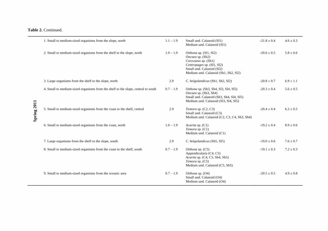
Table 2. Continued.

Sp

rin

g 2

01

1

1. Small to medium-sized organisms from the slope, north 1.1 – 1.9 Small und. Calanoid (Sl1) -21.8 ± 0.4 4.6 ± 0.3 Medium und. Calanoid (Sl1) 2. Small to medium-sized organisms from the shelf to the slope, north 1.0 – 1.9 Oithona sp. (Sl1, Sl2) -20.6 ± 0.5 5.8 ± 0.6 Oncaea sp. (Sh2) Corycaeus sp. (Sh1) Centropages sp. (Sl1, Sl2) Small und. Calanoid (Sl2) Medium und. Calanoid (Sh1, Sh2, Sl2) 3. Large organisms from the shelf to the slope, north 2.9 C. helgolandicus (Sh1, Sh2, Sl2) -20.8 ± 0.7 6.9 ± 1.1 4. Small to medium-sized organisms from the shelf to the slope, central to south 0.7 – 1.9 Oithona sp. (Sh3, Sh4, Sl3, Sl4, Sl5) -20.3 ± 0.4 5.6 ± 0.5 Oncaea sp. (Sh3, Sh4) Small und. Calanoid (Sh3, Sh4, Sl4, Sl5) Medium und. Calanoid (Sl3, Sl4, Sl5) 5. Small to medium-sized organisms from the coast to the shelf, central 2.9 Temora sp. (C2, C3) -20.4 ± 0.4 6.2 ± 0.5 Small und. Calanoid (C3) Medium und. Calanoid (C2, C3, C4, Sh3, Sh4) 6. Small to medium-sized organisms from the coast, north 1.0 – 1.9 Acartia sp. (C1) -19.2 ± 0.4 8.9 ± 0.6 Temora sp. (C1) Medium und. Calanoid (C1) 7. Large organisms from the shelf to the slope, south 2.9 C. helgolandicus (Sh5, Sl5) -19.0 ± 0.6 7.6 ± 0.7 8. Small to medium-sized organisms from the coast to the shelf, south 0.7 – 1.9 Oithona sp. (C5) -19.1 ± 0.3 7.2 ± 0.3 Appendicularia (C4, C5) Acartia sp. (C4, C5, Sh4, Sh5) Temora sp. (C5) Medium und. Calanoid (C5, Sh5) 9. Small to medium-sized organisms from the oceanic area 0.7 – 1.9 Oithona sp. (O4) -20.5 ± 0.5 4.9 ± 0.8 Small und. Calanoid (O4) Medium und. Calanoid (O4)

Table 2. Continued.

Au

tum

n 2

01

1

1. Large Decapod larvae from the shelf, north 3.5 Decapod larvae (Sh2) -20.3 ± 0.2 2.4 ± 0.2 2. Small to medium-sized organisms from the slope, north 0.7 – 1.9 Oithona sp. (Sl1) -20.5 ± 0.1 5.4 ± 0.9 Small und. Calanoids (Sl1) Medium und. Calanoids (Sl1) 3. Small to medium-sized organisms from the shelf to the slope, central to north 0.7 – 1.9 Oithona sp. (Sh2, Sl3) -20.5 ± 0.1 3.9 ± 0.4 Small und. Calanoids (Sl3) Medium und. Calanoids (Sh2, Sl3) 4. Small to medium-sized organisms from the coast to the shelf, north 0.7 – 1.9 Oncaea sp. (Sh1) -20.9 ± 0.0 7.0 ± 0.4 Temora sp. (Sh1) Medium und. Calanoids (Sh1) 5. Small to medium-sized organisms from the coast to the shelf, central 0.7 – 1.9 Oithona sp. (Sh3) -20.2 ± 0.2 6.2 ± 0.6 Oncaea sp. (C3, Sh3) Temora sp. (C3, Sh3) Medium und. Calanoids (Sh3) 6. Small to medium-sized organisms from the coast to the slope, south 0.7 – 1.9 Oithona sp. (Sl5) -20.3 ± 0.4 5.8 ± 0.7 Oncaea sp. (C4, C5, Sh4) Corycaeus sp. (C4) Small und. Calanoids (Sl5) Medium und. Calanoids (C4, C5, Sh4, Sl5)

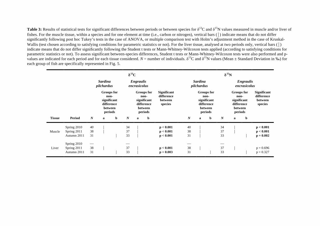
Table 3: Results of statistical tests for significant differences between periods or between species for !13C and !15N values measured in muscle and/or liver of fishes. For the muscle tissue, within a species and for one element at time (i.e., carbon or nitrogen), vertical bars (!) indicate means that do not differ significantly following post hoc Tukey’s tests in the case of ANOVA, or multiple comparison test with Holm’s adjustment method in the case of Kruskal-Wallis (test chosen according to satisfying conditions for parametric statistics or not). For the liver tissue, analysed at two periods only, vertical bars (!) indicate means that do not differ significantly following the Student t tests or Mann-Whitney-Wilcoxon tests applied (according to satisfying conditions for parametric statistics or not). To assess significant between-species differences, Student t tests or Mann-Whitney-Wilcoxon tests were also performed and p-values are indicated for each period and for each tissue considered. N = number of individuals. !13C and !15N values (Mean ± Standard Deviation in ‰) for each group of fish are specifically represented in Fig. 5.

"13C "15

N

Sardina

pilchardus

Engraulis

encrasicolus

Sardina

pilchardus

Engraulis

encrasicolus

Groups for

non-

significant

difference

between

periods

Groups for

non-

significant

difference

between

periods

Significant

difference

between

species

Groups for

non-

significant

difference

between

periods

Groups for

non-

significant

difference

between

periods

Significant

difference

between

species

Tissue Period N a b N a b N a b N a b

Muscle Spring 2010 40 ! 34 ! p < 0.001 40 ! 34 ! p < 0.001

Spring 2011 38 ! 37 ! p < 0.001 38 ! 37 ! p < 0.001

Autumn 2011 31 ! 33 ! p < 0.001 31 ! 33 ! p = 0.002

Liver Spring 2010 # # # # Spring 2011 38 ! 37 ! p < 0.001 38 ! 37 ! p = 0.696 Autumn 2011 31 ! 33 ! p = 0.003 31 ! 33 ! p = 0.327

Table 4: Summary of estimated contributions (Mean values ± Standard Deviation in %) of mesozooplanktonic prey groups in the diet of European sardine Sardina pilchardus and European anchovy Engraulis encrasicolus resulting from the different mixing models applied with different Trophic Enrichment Factors (TEFs: !"13C and !"15N) taken from the literature (i.e., sensitivity analysis). Values for groups of prey contributing on average to more than 10% in the diet of each species, when the four models performed by species and by tissue are considered, are in bold. For signification of each group of prey within each period, see Table 2.

Model applied Model 1 Model 2 Model 3 Model 4 Model 1 Model 2 Model 3 Model 4

References for

TEFs

Post 2002 Sweeting et al.

2007ab

Pinnegar and

Polunin 1999

Trueman

et al. 2005

Mean ± SD Post 2002 Sweeting et al.

2007ab

Pinnegar and

Polunin 1999

Trueman et

al. 2005

Mean ± SD

!"13

C 0.4 ± 1.3 1.7 ± 1.1 2.5 ± 0.1 2.1 ± 0.1 0.4 ± 1.3 0.9 ± 1.3 1.2 ± 0.8 1.6 ± 0.3 Period !"

15N 3.4 ± 1.0 3.2 ± 1.3 3.3 ± 0.2 2.3 ± 0.3 3.4 ± 1.0 2.3 ± 0.9 2.2 ± 0.2 0.0 ± 0.3

Sp

rin

g 2

010

Sardina pilchardus (n = 40)

Prey group MUSCLE LIVER

1 1.2 ± 1.0 1.3 ± 1.2 1.1 ± 1.0 1.7 ± 1.6 1.3 ± 0.3 ! ! ! ! !

2 2.1 ± 1.8 3.0 ± 2.7 1.3 ± 1.2 3.1 ± 3.0 2.4 ± 0.8 ! ! ! ! ! 3 0.9 ± 0.8 0.9 ± 0.8 1.1 ± 1.0 1.3 ± 1.2 1.1 ± 0.2 ! ! ! ! ! 4 34.5 ± 12.5 38.0 ± 9.3 16.4 ± 10.6 26.5 ± 12.7 28.9 ± 9.6 ! ! ! ! !

5 10.3 ± 8.3 9.6 ± 5.9 28.9 ± 11.7 9.9 ± 6.5 14.7 ± 9.5 ! ! ! ! !

6 2.1 ± 2.0 1.7 ± 1.4 10.7 ± 4.5 2.3 ± 1.8 4.2 ± 4.3 ! ! ! ! ! 7 3.3 ± 3.0 3.8 ± 3.2 3.7 ± 3.4 4.5 ± 4.1 3.8 ± 0.5 ! ! ! ! !

8 45.6 ± 11.8 41.7 ± 8.3 36.8 ± 13.1 50.7 ± 12.8 43.7 ± 5.9 ! ! ! ! !

Engraulis encrasicolus (n = 34)

MUSCLE

LIVER

1 4.0 ± 3.5 5.5 ± 3.8 5.2 ± 4.0 1.4 ± 1.3 4.0 ± 1.9 ! ! ! ! !

2 26.0 ± 7.2 12.5 ± 5.3 4.9 ± 4.0 1.7 ± 1.6 11.3 ± 10.8 ! ! ! ! ! 3 1.7 ± 1.6 3.4 ± 2.6 8.2 ± 5.2 1.5 ± 1.4 3.7 ± 3.1 ! ! ! ! ! 4 27.9 ± 11.4 23.1 ± 6.7 10.7 ± 7.7 15.6 ± 10.3 19.3 ± 7.7 ! ! ! ! !

5 6.0 ± 5.4 15.1 ± 6.2 19.3 ± 11.1 30.1 ± 13.3 17.6 ± 10.0 ! ! ! ! !

6 1.7 ± 1.7 6.4 ± 3.7 28.5 ± 6.2 15.9 ± 5.3 13.1 ± 11.8 ! ! ! ! !

7 6.0 ± 5.4 12.0 ± 6.2 11.6 ± 8.5 4.8 ± 4.6 8.6 ± 3.7 ! ! ! ! !

8 26.7 ± 10.2 22.0 ± 6.2 11.6 ± 7.8 29.0 ± 12.5 22.3 ± 7.7 ! ! ! ! !

Table 4. Continued.

Sp

rin

g 2

011

Sardina pilchardus (n = 38)

Prey group MUSCLE LIVER

1 1.5 ± 1.4 2.1 ± 1.7 11.0 ± 4.6 2.3 ± 2.2 4.2 ± 4.5 6.0 ± 5.1 6.2 ± 4.2 9.1 ± 5.8 3.0 ± 5.2 6.1 ± 2.5 2 3.4 ± 2.9 5.0 ± 3.3 3.6 ± 3.2 1.9 ± 1.8 3.5 ± 1.3 7.7 ± 6.1 9.9 ± 5.9 9.9 ± 7.1 2.3 ± 3.4 7.5 ± 3.6 3 3.3 ± 2.7 8.6 ± 4.0 32.7 ± 5.7 25.0 ± 5.0 17.4 ± 13.8 2.2 ± 2.0 8.4 ± 5.1 19.9 ± 8.3 11.0 ± 16.7 10.4 ± 7.3

4 4.2 ± 3.2 4.8 ± 3.2 1.9 ± 1.7 1.3 ± 1.3 3.1 ± 1.7 19.8 ± 9.5 11.0 ± 6.0 7.8 ± 6.0 1.7 ± 2.3 10.1 ± 7.5

5 4.3 ± 3.4 7.3 ± 4.2 4.4 ± 3.7 2.2 ± 2.2 4.6 ± 2.1 6.2 ± 5.1 10.5 ± 6.1 10.3 ± 7.3 2.7 ± 3.7 7.4 ± 3.7 6 27.2 ± 5.2 31.6 ± 4.0 41.3 ± 4.6 63.1 ± 5.5 40.8 ± 16.0 2.0 ± 1.8 14.6 ± 4.8 18.0 ± 6.3 73.0 ± 27.1 26.9 ± 31.5

7 25.4 ± 7.0 19.2 ± 4.8 2.0 ± 1.8 1.7 ± 1.6 12.1 ± 12.1 8.1 ± 5.6 14.5 ± 5.8 10.2 ± 6.7 2.7 ± 2.6 8.9 ± 4.9 8 27.7 ± 7.7 18.5 ± 5.2 1.7 ± 1.5 1.5 ± 1.5 12.4 ± 13.0 14.4 ± 7.5 15.1 ± 6.0 8.5 ± 6.0 2.2 ± 2.3 10.1 ± 6.0

9 3.0 ± 2.4 2.9 ± 2.2 1.4 ± 1.3 1.0 ± 0.9 2.1 ± 1.0 33.6 ± 7.7 9.8 ± 5.4 6.3 ± 5.0 1.4 ± 1.9 12.8 ± 14.3

Engraulis encrasicolus (n = 37)

MUSCLE

LIVER

1 2.5 ± 2.3 12.8 ± 5.8 24.9 ± 7.0 6.2 ± 5.1 11.6 ± 9.8 9.6 ± 6.5 15.8 ± 7.6 15.1 ± 7.9 4.0 ± 7.2 11.1 ± 5.5

2 4.9 ± 4.5 10.9 ± 6.6 5.7 ± 5.1 4.0 ± 3.7 6.4 ± 3.1 9.8 ± 7.4 10.0 ± 7.4 7.8 ± 6.4 3.0 ± 3.5 7.7 ± 3.3 3 2.2 ± 2.1 15.4 ± 6.4 46.6 ± 10.9 54.3 ± 12.0 29.6 ± 24.8 3.8 ± 3.3 25.3 ± 10.6 40.4 ± 14.5 11.4 ± 13.1 20.2 ± 16.1

4 10.2 ± 7.5 9.1 ± 6.1 3.5 ± 3.1 2.6 ± 2.4 6.4 ± 3.9 17.3 ± 10.8 6.8 ± 5.6 5.0 ± 4.4 2.3 ± 2.5 7.9 ± 6.6 5 4.9 ± 4.4 11.2 ± 6.7 5.7 ± 5.2 4.5 ± 4.0 6.6 ± 3.1 8.1 ± 6.6 10.6 ± 7.7 8.1 ± 6.6 3.4 ± 3.6 7.6 ± 3.0 6 3.5 ± 3.2 14.7 ± 5.6 5.8 ± 4.6 20.9 ± 7.6 11.2 ± 8.1 2.8 ± 2.4 14.2 ± 6.7 11.3 ± 7.0 67.1 ± 22.5 23.9 ± 29.2

7 23.4 ± 11.6 9.2 ± 5.8 2.5 ± 2.2 2.9 ± 2.7 9.5 ± 9.8 6.5 ± 4.8 6.1 ± 5.0 4.2 ± 3.8 3.9 ± 3.7 5.2 ± 1.3 8 33.2 ± 13.1 8.6 ± 5.7 2.3 ± 2.2 2.5 ± 2.3 11.7 ± 14.7 8.7 ± 6.1 5.5 ± 4.6 3.9 ± 3.5 3.0 ± 2.9 5.3 ± 2.5 9 15.2 ± 7.6 8.1 ± 5.6 3.0 ± 2.8 2.1 ± 1.9 7.1 ± 6.0 33.4 ± 10.6 5.7 ± 4.8 4.2 ± 3.8 1.9 ± 2.0 11.3 ± 14.8

Table 4. Continued.

Au

tum

n 2

011

Sardina pilchardus (n = 31)

Prey group MUSCLE LIVER

1 1.1 ± 1.1 2.1 ± 2.0 2.6 ± 2.4 2.7 ± 2.7 2.1 ± 0.7 1.7 ± 1.5 1.6 ± 1.6 1.3 ± 1.2 2.4 ± 2.3 1.8 ± 0.5

2 3.7 ± 3.6 7.2 ± 6.4 6.9 ± 6.1 5.7 ± 5.4 5.9 ± 1.6 6.6 ± 5.6 7.2 ± 6.4 4.5 ± 4.4 6.8 ± 6.4 6.3 ± 1.2 3 1.7 ± 1.6 2.9 ± 2.8 4.1 ± 3.8 3.1 ± 3.0 3.0 ± 1.0 2.6 ± 2.3 2.6 ± 2.5 2.0 ± 1.9 3.7 ± 3.7 2.7 ± 0.7

4 73.2 ± 15.7 17.3 ± 11.8 73.5 ± 10.4 4.7 ± 4.2 42.2 ± 36.4 28.4 ± 11.1 45.8 ± 14.5 67.3 ± 12.1 73.4 ± 11.1 53.7 ± 20.6

5 14.1 ± 13.0 50.9 ± 12.5 6.5 ± 6.0 65.8 ± 15.9 34.3 ± 28.6 43.2 ± 13.1 28.5 ± 11.4 17.4 ± 10.9 7.0 ± 6.2 24.0 ± 15.5

6 6.2 ± 6.2 19.6 ± 12.9 6.4 ± 5.7 18.0 ± 14.3 12.6 ± 7.2 17.5 ± 11.1 14.3 ± 9.7 7.5 ± 6.7 6.7 ± 6.1 11.5 ± 5.3

Engraulis encrasicolus (n = 33)

MUSCLE

LIVER

1 3.2 ± 3.0 3.1 ± 2.9 2.6 ± 2.4 2.5 ± 2.4 2.9 ± 0.4 5.2 ± 4.3 3.2 ± 2.9 2.3 ± 2.1 2.1 ± 2.0 3.2 ± 1.4

2 10.4 ± 8.8 11.3 ± 9.2 6.9 ± 6.1 8.0 ± 7.2 9.2 ± 2.0 15.8 ± 9.1 14.6 ± 8.7 7.1 ± 5.9 5.1 ± 4.9 10.7 ± 5.3

3 4.6 ± 4.3 4.8 ± 4.5 4.1 ± 3.8 4.0 ± 3.8 4.4 ± 0.4 7.8 ± 6.1 5.9 ± 5.0 3.6 ± 3.3 3.3 ± 3.3 5.2 ± 2.1 4 18.6 ± 12.7 33.1 ± 12.3 73.5 ± 10.4 63.1 ± 13.5 47.1 ± 25.6 20.1 ± 8.6 38.8 ± 9.3 72.8 ± 8.0 80.1 ± 9.3 53.0 ± 28.3

5 42.5 ± 18.0 29.0 ± 13.1 6.5 ± 6.0 12.4 ± 9.5 22.6 ± 16.3 28.6 ± 9.3 21.2 ± 9.3 7.6 ± 6.0 4.7 ± 4.6 15.5 ± 11.3

6 20.7 ± 13.3 18.7 ± 12.0 6.4 ± 5.7 10.0 ± 8.4 14.0 ± 6.8 22.5 ± 9.4 16.3 ± 8.8 6.6 ± 5.4 4.7 ± 4.7 12.5 ± 8.4

Fig. 1: Maps of the study area (Bay of Biscay), indicating the transects realised from the coastline to the slope and the stations selected for plankton sampling for the three periods considered in this study: A) Spring 2010, B) Spring 2011 and C) Autumn 2011. Trawls for fish sampling are also indicated. T = Transect; C = Coast; Sh = Shelf; Sl = Slope; O = Oceanic. The study area represented (outlines of the box) extends from 0° to 8°W and from 43°N to 48°N (Source: Etopo1 NOAA – LIENSs – 2013. Design and realization: Cellule Géomatique LIENSs – UMR 7266).

Fig. 2: Histograms presenting the percentage of copepods and of other taxa (relative to the total abundance of mesozooplanktonic organisms, in number of individuals. m-3) for each station selected and considered for taxonomic identification in A) Spring 2010, B) Spring 2011 and C) Autumn 2011. C = Coast; Sh = Shelf; Sl = Slope; O = Oceanic; see Fig. 1 for the corresponding location of each station.

Fig. 3: Results of the taxonomic identification performed on mesozooplankton samples collected in A) Spring 2010, B) Spring 2011 and C) Autumn 2011. The number above a pie corresponds to the total abundance of organisms within a station (in number of individuals. m-3), and the size of pies is proportional to the total abundance. Among the ‘dominant taxa’ (see text), small organisms are represented in shades of red to yellow, medium-sized organisms in shades of green, and large organisms in shades of blue (see Table 1). Within each station, the proportion of taxa in minor proportion (i.e., with an abundance < 5% when taken individually, and therefore not analysed for stable isotope ratios – see text) is indicated in black. The study area represented (outlines of the box) extends from 0° to 8°W and from 43°N to 48°N (Source: Etopo1 NOAA – LIENSs – 2013. Design and realization: Cellule Géomatique LIENSs – UMR 7266).

Fig. 4: Stacked bar charts presenting A) the frequency of identified organisms belonging to small, medium-sized or large organisms within each of the three periods considered in this study, all stations considered together over the Bay of Biscay; B) the frequency of organisms identified in coastal stations, stations from the shelf or stations from the slope and oceanic stations within each of the three periods considered in this study, all sizes considered together. Only organisms belonging to ‘dominant taxa’ were taken into account for both histograms (see text).

Fig. 5: !13C and !15N values (mean ± SD, in ‰) for European sardine Sardina pilchardus and European anchovy Engraulis encrasicolus, depending on the period considered and on the tissue analysed. Detailed results of statistical tests for significant difference between species or between periods for a given tissue or for a given element are presented in Table 3. The dotted line is only drawn as a guide to visually distinguish muscle and liver tissue values that are presented here on the same figure.