SMA Technical Memo #166 - · era of wideband SMA. This technical memo reports a progress of Miriad...

SMA Technical Memo #166

Subject: A METHOD FOR HANDLING SMA DATA FROM SWARMCORRELATOR -Solving for bandpass of high- or full- spectral resolution data

Date: October 2, 2017$

From: Jun-Hui Zhao (SAO)

___________________$Updated from the versions since February 25, 2016; Submitted September 21, 2017

Abstract -

Along with the wideband development for SMA, we are implementing Miriad[1] software to accommodate large volumes of SMA data. For the reduction of high spectral resolution and wideband data generated from SMA observations with the newly upgraded SWARM correlator, a considerable amount of software upgrading and further development is indispensable concerning software infrastructure and advanced algorithms in the era of wideband SMA. This technical memo reports a progress of Miriad softwaredevelopment for the reduction of SWARM data, specifically for the program of bandpass corrections. Given a general calibrator, the effects owing to emission structure and variability of sources are discussed along with a visibility model. A method of separating between the distortion functions in terms of complex antenna gains, instrumental bandpass, and residual delays is also discussed. This method has been applied to Miriad software. Three processes prior to passing the data to the bandpass solver are discribed: (1) visibility weighting in both variance and source structure, (2) normalization, and (3) enhancement of signal-to-noise ratio with moving smoothing and/or orthogonal polynomials' fitting algorithms. The relevant subroutines have been implemented in the Miriad task smamfcal. A test data set was produced on February 11, 2016 from observations of Sgr B2 North, a site of forming a massive star cluster, producing four sub-band of high-resolution spectral data (0.1 MHz/channel) with a part of the SWARM correlator. An example for reduction of SWARM data, utilizing the method described in this technical memo, is demonstrated based on the test data.

1. Motivation -

As the SMA SWARM correlator comes online, reliable bandpass corrections become a pressing issue for probing fine structure of kinematics in imaging molecular lines with a high spectral-resolution as well as for imaging comprehensive distributions of continuum emission sampled with wideband (WB) data. For some special objects, the line width appears to be narrow; for example, the velocity widths of molecular lines from brown dwarf or proto brown dwarf candidates are as narrow as 1 km/s or even less[2,3,4]. The full spectral resolution, 0.1 MHz per channel or 0.1 km/s at 1 mm, provided by the SWARM correlator is needed for the study of the narrow line systems. However, a poor signal-to-noise ratio (S/N) provided for such high-spectral resolution data becomes an issue in solving for a reliable bandpass, given a lack of strong QSOs at higher frequencies and highly variable cores of blazars in the range of wavelengths covered in the radio, millimeter and submillimeter (RMS) bands as well as extended structures of disc-like emission from strong thermal objects in the Solar system. The bandpass solvers that were developed early need to be upgraded with more advanced algorithms

SMA Technical Memo https://www.cfa.harvard.edu/sma/miriad/swarm/...

1 of 17 10/02/2017 02:12 PM

to address the inadequate budget in S/N for both spectrally and angularly high resolution observations at submillimeter wavelengths. On other hand, wideband continuum imaging employs the multiple-frequency synthesis (MFS) imaging technique[5], which requires well-calibrated data across the sampled spectral band. In addition to bandpass and delay corrections, the phase between individual spectral chunks or sub-bands (hereafter) must be aligned well and also corrections for time-dependent residual delays need to be carried out in order to achieve high-dynamic range images; both errors in phase become critical issues in sub-arcsec resolution imaging. The relevant algorithms have been developed and implemented in Miriad software. The goal of the efforts is to match the specifications required by a variety of science cases in the reduction of wideband data produced from the SMA SWARM correlator.

In Section 2, a visibility model for a celestial object is discussed concerning calibrations. In Section 3, a method of pre-processing data prior to solving for antenna-based bandpass as well as auto-editing the bandpass solutions are described and discussed. The relevant algorithms have been implemented in a Miriad program smamfcal. Sections 4 and 5 give the in-line document from help deck of smamfcal, and a usage for setting up variables in a c-shell script, respectively. A test data set was given from SMA observations of Sgr B2 North on Feburary 11, 2016 with four SWARM sub-bands. Application and demonstration for this software technique with the test data are given in Section 6. The names of relevant subroutines and functions for SMA Miriad implementation are given in Appendix.

2. Visibility model -

In the era of new generation interferometer arrays at RMS wavelengths with a capability of wideband sampling, telescope sensitivities in detections of weaker objects have been dramatically improved in recent years. Source structure and variability of a celestial object used as a calibrator become noticeable issues in data calibration and imaging. Previous assumptions of point source models for core-dominant QSOs or blazars in data calibrations appear to be inappropriate, and the issues owing to the nature of sources require special attention and treatment. A visibility function in modeling a calibrator concerning its variability and structure is introduced and discussed. A transformation of actual source structure into a pseudo point-source model and a process of removal of time variability are reviewed as follows.

2.1. Structure and variability Given a (u, v) plane, observing frequency ν, and time t, a visibility function sampled with a wideband interferometer array towards a target source, in general, can be expressed as:

V(u, v, ν, t) = VS(u, v, ν, t) e2πiντA GA(ν, t), (2.1)

where GA(ν, t) and τA correspond to time-dependent complex gains and a delay causedby both instrumental errors and atmospheric effects, respectively; both terms are antenna-based. For a QSO or a blazar, its source function can be simply described as a core-dominant source with a strong point-like function in the (u, v) plane, VC(u, v, ν, t), an initial model separated from the extended emission structure VExt(u, v, ν), namely:

VS(u, v, ν, t) = VC(u, v, ν, t) + VExt(u, v, ν). (2.2)

For a planet in the Solar system, the visibility function becomes:


2 of 17 10/02/2017 02:12 PM

VS(u, v, ν, t) = VExt(u, v, ν), (2.3)

assuming that time variability in both the distribution of emission brightness over a planet disc and the total intensity can be ignored during an observing period.

2.2. Source model and creation of pseudo point source As improvement of an interferometer array in both sensitivity and angular resolution,the previous assumption of a calibrator (a QSO or a small planet) as a point sourceis no longer suitable. The extended structure and variability of a calibrator appear to generate significant effects, leading to limitations in both calibration precision and quality of interferometer imaging. Given a celestial object, a time-invariant or a stable structure of its emission can be constructed as shown in radio observations and wideband imaging[6]. Then, a model for the structure of stable emission from a calibrator can be expressed as:

VS(u, v, ν) = VC(u, v, ν) + VExt(u, v, ν). (2.4)

In principal, given a calibrator, a pseudo-point visibility function modulated by atmospheric attenuation and delay as well as antenna-based instrumental effects can be formed by the sampled visibilities, Eq(2.1), divided by the relevant model of the stable emission structure Eq(2.4): VP(u, v, ν, t) = V(u, v, ν, t) / VS(u, v, ν). (2.5)

For a QSO with a variable intensity I0+ΔI(t) of the radiation from its core which is assumed to be placed at the phase center, Eq (2.5) can be expressed as,

VP(u, v, ν, t) = {1 + ΔI(t)/[I0 + VExt(u, v, ν)]}e2πiντA GA(ν, t), (2.6)

where the spectrum of the core is further assumed to be flat for simplicity. The term caused by time-variable radiation from the core requires a special process to remove it prior to further complex gain calibration[6]. For a planet or a calibrator with no time-variability issues,

VP(u, v, ν, t) = e2πiντA GA(ν, t). (2.7) And the antenna-based delay can be further written as, τA = τ0 + Δτ. (2.8)

For the SMA concern, τ0 is assumed to be removed by an on-line process and Δτis the residual delay that depends on time. Furthermore, the frequency-dependent and time-dependent functions in the complex gain can be decoupled if the instrumental bandpass is stable enough,

GA( ν, t) = gA(t) gB(ν). (2.9)

Thus, Eq(2.7) can be re-written to, VP(u, v, ν, t) = gA(t) gB(ν)e2πiν Δτ. (2.10)


3 of 17 10/02/2017 02:12 PM

The rest of this technical memo discusses a method of corrections for bandpassterm gB(ν) and residual delay Δτ. It is obvious that the normalization process using the mean visibility over a sub-band at a time interval of an integration record discussed in section 3.2 effectively eliminates the term gA(t). The function of the pseudo-point source normalized by each of the pseudo-continuum integrations for each baseline describes the solutions for bandpass shape and residual delays, i.e.,

VP(ν, t) = gB(ν)e2πiν Δτ. (2.11)

We also note that normalization of the visibility data divided by a baseline-based pseudo-continuum at each integration time interval can eliminate the variability of the core emission in the case of a blazar, which is described in Eq(2.6). Before discussion of the detailed algorithm for a wideband bandpass in next section, caveats for the visibility model discussed above are noted:

1) A perfect source model for the stable emission Eq(2.4) is assumed. In practice, at the submillimeter wavelengths, efforts to build reliable models for relevant calibrators are needed.

2) In the equations from Eq(2.1) to Eq(2.11), the visibility and the relevant modulation models are assumed to be continuous functions of the variables u, v, ν, t. In the sampling process of an interferometer array, the sampled data are discrete. Thus, in computer programming, the formulas need to be written in a numerical way, e.g., Eq(2.10) and Eq(2.11) can be re-written as:

VPij(νk,tl) = gAij(tl)gBij(νk)e2πiνkΔτij(νk,tl) (2.12)

and

VPij(νk,tl) = gBij(νk)e2πiνkΔτij(νk,tl). (2.13)

3) The indices i, j, k, and l are integers; the antenna pair or baseline indices i and j are from 0 to nA-1, and nA is a number of antennas used in an array; the frequency index k is in the range between 0 and nchan-1 that is a total number of spectral channels sampled by a correlator; the time sampling or integration index l is from 0 to nt-1, where nt is a total number of time sampling intervals used for the calibrators given a data set.

4) The next section is to present a method of pre-processing the visibility data to optimize the ratio of signal-to-noise for solving antenna-based complex bandpass gB as well as antenna-based residual delay Δτ which may be also dependent on sub-bands in the case of multiple sub-bands used for wideband spectral sampling. The two terms can be decoupled if the instrumental bandpass does not change over a relevant period of data sampling. Then, the instrumental bandpass term can be corrected with solutions derived from the data acquired in a snapshot observation of a strong calibrator.

5) The residual delay Δτ may be a small quantity and frequently varies in time. Phase slopes produced from this term in sub-bands generate noticeable artifacts near a strong compact source in high-angular resolution images, limiting dynamic range of imaging[6]. The algorithm discussed in Section 3 provides a way to derive solutions in phase caused by the residual delays. Linear fitting to the phase slopes as function of frequency over each of the sub-bands may be carried out to


4 of 17 10/02/2017 02:12 PM

derive solutions for residual delays in the case of poor S/N, given a time interval. For high S/N data, the phase solutions can be directly applied to a target source.

3. Bandpass solver SMAmfcal -

The program smamfcal is a Miriad task which determines calibration solutions for antenna-based corrections in aspects of antenna gains, delay terms and passband shapes from a multi-frequency observation. This task is developed based on the original Miriad program mfcal coded by Bob Sault according to the Miriad code signature. In the past decade, smamfcal has been powered by implementing new algorithms as discussed below for handling poor S/N data from observations at submillimter wavelengths. The algorithm of matrix solver in mfcal is retained in smamfcal. The algorithms used for pre-processing visivilities and editing bandpass solutions are listed below along with descriptions and discussions in the following sub-sections.

3.1 WeightIn addition to uniform weighting, two methods of visibility weighting have been implemented in smamfcal: 1) use variance (σ2) of visibility; 2) use amplitude (A) of visibility, usually with the n-th power of the amplitude (An and n>1). The second method is dependent on the source structure, less weighting the contribution from the visibilities with lower S/N data due to the emission structure in a resolved or a partially-resolved source. A subroutine accumwt accumulates the visibility weight in paralle to the visibility accumulation with one-to-one mapping for each data point. Three options have been provided for weighting in smamfcal:

1. weight = 1/σ2 or 1, the same way as that used in mfcal2. weight = 1/(A/σ)2

3. weight = 1/(A/σ)4

Option 3 can effectively give less weighting to the lower S/N visibilities near nulls for a disc-like object.

3.2. NormalizationSolving bandpass is usually carried out before phase corrections are made. A pseudo continuum visibility is computed by vector averaging each sub-band at a time of each integration record. A normalization of the visibility for each spectral channel is carried out with the pseudo continuum visibility. Thus, such a self-normalization can remove any temporal phase drifts while retaining bandpass variations across a sub-band. The normalization is accomplished with two subroutines avgchn and divchz. The former determines the vector average of spectral visibilities in the basis of per baseline and per sub-band given an integration. Then, a normalized spectrum is computed.

For a calibrator partially resolved or with extended emission rather than a point source, its visibilites need to be normalized by a model of its emission structure before processing in smamfcal. As discussed in Section 2, the normalization of the emission-structure model will remove the calibrator phase structure across the frequency band within which the data are sampled. The issues concerning calibrator structure become more critical for wideband data at the RMS wavelengths when the overall sensitivity gets better. A catalog for calibrator models needs to be built so that an automatic normalization with an emission-structure model can be programmed given a relevant calibrator.


5 of 17 10/02/2017 02:12 PM

3.3. Smooth and LSQ fit The subroutine smoothply hosts two micro-processes, i.e. moving smooth[4] and orthogonal polynomials' fitting[4] to each of the visibility spectra prior to solving for bandpass. Options msmooth and opolyfit are given for users to select one of the two micro-processes to handle poor S/N spectral data. For high spectral resolution data, such as SWARM data, msmooth appears to be a better choice.The algorithm of msmooth is discussed as follows.

For a sub-band with a total number of channels n, the complex quantity in each channel visibility consists of two parts, the true value of the measured quantity η and a measurement error ε,

yi = ηi+εi, i = 1, 2, ..., n (3.1)

We assume that ηi is a polynomial in frequency ν and the error εi to be normally distributed about zero. In the high-spectral resolution case δν ~ 0.1 MHz, such as in the spectral production from the SMA SWARM correlator, the variation trend ηiis often embedded in the fluctuation of error εi for most of QSOs at submillimter wavelengths. Thus a smoother function of ν is needed to replace every value of yi,

i+k

ui = Σyi / (2k+1), (3.2) j=i-k

If η is a linear function of ν in the frequency interval Δν = νi+k-νi-k = (2k+1) δν,

ηj = α + βνj, j = −k, −k+1, ..., k (3.3)

α and β are constant. They can be determined from the data by linear regression. For a higher order polynominal η,

ηj = a1 + a2νj + a3νj2 + ... + al+1νjl, (3.4)

The coefficients of the polynomial function can be determined from the data by least square fitting to the smoother function ui, Eq(3.2).

If the variance of yi is σ2, then the variance corresponding to the smoother function ui is,

σu2 = σ2/(2k+1), (3.5)

The ratio of the variance from the original data to that of the smoother function is proportional to (2k+1),

σ2/σu2 = 2k+1, (3.6)

For k=5, the variance of a spectral smoother is an order in magnitude smaller than that of the original spectrum. The default provided in smamfcal for moving smooth is k=3 and linear regression l=1. For the SWARM spectra, the linear regression approaching appears to be appropriate for even larger value of k. For the trial data used in Section 6, a smoother with k=7 is applied. The pre-process for options=msmoothin smamfcal should be adequate in solving for the bandpass trend of a telescope with data taken from a relatively weak calibrator. For SMA SWARM high-spectral


6 of 17 10/02/2017 02:12 PM

resolution sub-bands, a smoother with k=10 can greatly enhance S/N ratio of the spectral data while a slow variation of bandpass response is retained. Thus with the pre-process of moving smooth, we can correct for the bandpass of SWARM spectral data with a high confidence level.

3.4. Auto-editing bandpass solutions Solutions of bandpass may be contaminated due to individual channels with large errors, e.g. spectral spikes produced from an instrumental part of a telescope. A function for auto-editing of bandpass solutions is implemented, which rejects solutions that are highly deviated from the actual bandpass trend; and replacements can be made with the values derived from orthogonal polynomials' fitting to overall solutions.

4. Help deck -

Task: smamfcal

Responsible: Jun-Hui Zhao

SmaMfCal is a Miriad task which determines calibration corrections (antenna gains, delay terms and passband shapes) from a multi-frequency observation. The delays and passband are determined from an average of all the selected data. The gains are worked out periodically depending upon the user selected interval. SmaMfcal implements algorithms for weighting, continuum vector normalization, and moving smooth prior to solving for bandpass and gains, which are necessary for handling data at submillimeter wavelength when the S/N is poor and phase dispersion is large. The basic solving algorithms are the same as in MfCal.

Keyword: vis Input visibility data file. No default. This can (indeed should) contain multiple channels and spectral windows. The frequency set-up can vary with time.

Keyword: line Standard line parameter, with standard defaults.

Keyword: edge The number of channels, at the edges of each spectral window, that are to be dropped. Either one or two numbers can be given, being the number of channels at the start and end of each spectral window to be dropped. If only one number is given, then this number of channels is dropped from both the start and end. The default value is 0.

Keyword: select Standard uv selection. Default is all data.

Keyword: flux Three numbers, giving the source flux, the reference frequency (in GHz) and the source spectral index. The flux and spectral index are at the reference frequency. If no values are given, then SmaMfCal


7 of 17 10/02/2017 02:12 PM

checks whether the source is one of its known sources, and uses the appropriate flux variation with frequency. Otherwise the default flux is determined so that the rms gain amplitude is 1, and the default spectral index is 0. The default reference frequency is the mean of the frequencies in the input data. Also see the `oldflux' option. (This function has not been implemented for SMA data).

Keyword: refant The reference antenna. Default is 3. The reference antenna needs to be present throughout the observation. Any solution intervals where the reference antenna is missing are discarded.

Keyword: minants The minimum number of antennae that must be present before a solution is attempted. Default is 2.

Keyword: interval This gives one or two numbers, both given in minutes, both being used to determine the extents of the gains calibration solution interval. The first gives the max length of a solution interval. The second gives the max gap size in a solution interval. A new solution interval is started when either the max times length is exceeded, or a gap larger than the max gap is encountered. The default max length is 5 minutes, and the max gap size is the same as the max length.

Keyword: weight This gives different ways to determine weights (wt) prior to solving for bandpass: -1 -> wt = 1; the same weighting method as used in MfCal. 1 -> wt ~ amp0**2/var(i); for a normalized channel visibility, the reduced variance is proportional to amp0**2/var(i), where amp0 is the amplitude of the pseudo continuum and var(i) is the variance of visibility for the ith channel. 2 -> wt ~ amp0**4/var(i)**2; Default is 2 for SMA and -1 for other telescopes. if you have stable phase, use -1; if the phase stability is poor, use 1 or 2; for a larger planet, 2 is recommended.

For antenna gains' solver: -1 -> wt = 1; the same weight method that is used in MfCal. >0 -> wt = 1/var, where var is the visibility variance. Defualt is 1/var.

Keyword: options Extra processing options. Several values can be given, separated by commas. Minimum match is used. Possible values are: delay Attempt to solve for the delay parameters. This can be a large sink of CPU time. nopassol Do not solve for bandpass shape. In this case if a bandpass table is present in the visibility data-set, then it will be applied to the data. interpolate Interpolate (and extrapolate) via a spline fit (to the real and imaginary parts) bandpass values for


8 of 17 10/02/2017 02:12 PM

channels with no solution (because of flagging). If less than 50% of the channels are unflagged, the interpolation (extrapolation) is not done and those channels will not have a bandpass solution. oldflux This causes SmaMfCal to use a pre-August 1994 ATCA flux density scale. See the help on "oldflux" for more information. (not relevant to SMA data) msmooth Do a moving average of the uv data (the real and imaginary parts) using the keyword smooth parameters specified prior to solving for bandpass. opolyfit Do a least-square fit to the bandpass solutions (the real and imaginary parts) with an orthogonal polynomial of degree n which can be given in keyword polyfit. wrap Don't unwrap phase while doing fit or smoothing the uv data. averrll In the case of solving for bandpass of dual polarizations, averrll gives vector average of rr and ll bandpass solutions; the mean value is written into the bandpass table for each of rr and ll.

Keyword: smooth This gives three parameters of moving smooth calculation of the bandpass/gain curves: smooth(1) = K parameter k giving the length 2k+1 of the averaging interval; default is 3. smooth(2) = L order of the averaging polynomial l; default is 1. smooth(3) = P probability P for computing the confidence limits; default is 0.9.

Keyword: polyfit polyfit gives a degree of orthogonal polynomial in least-sqaure fit to the bandpass/gain curves. Default is 3. polyfit: 1 (linear), 2 (parabolic), 3 (cubic), ....

Keyword: tol Solution convergence tolerance. Default is 0.001.

5. Usage -

The reduction of SMA data has been suggested to use msmooth in bandpass calibration, e.g.CalibrationProcedure₤ for data produced from the ASIC correlator. The function msmoothappears to be critical in solving high-spectral resolution bandpass of ASIC data. This pre-process appears to be essential for handling the high-spectral resolution SWARMdata. Here, an example is given for a usage of smamfcal in a C-shell script if one uses a QSO as a bandpass calibrator:

#!/bin/csh -fset fname = 160211_rx0.lsbset bcal = 3c273set edge = 500set refant = 1


9 of 17 10/02/2017 02:12 PM

set smooth = 7,1,0.9... (see CalibrationProcedure₤) smamfcal vis=$fname.swarm.tsys select='source('$bcal')' edge=$edge,$edge \ refant=$refant interval=1000000 options=msmooth smooth=$smooth

___________________₤https://www.cfa.harvard.edu/sma/miriad/swarm/pscripts/swarmcali_a.csh.html

6. Application & Testing -

Using a recent test data from the observation track on February 11, 2016 with a hybrid configuration of both ASIC and SWARM correlators. This is the first real data set that was produced from a part of the SWARM correlator, consisting of four high-resolution sub-band while the SMA was in an array of five antennas. Here is a report for the lower-side band (LSB) data set, which is produced with uvindex:

6.1. Description of the testing track on 2016-02-11

UVINDEX: version 5-sept-2013

Summary listing for data-set 160211_rx0.lsb

----------------------------------------------- Time Source Antennas Spectral Wideband Freq Record Name Channels Channels Config No.

16FEB11:17:20:13.8 3c273 8 71681 0 1 116FEB11:17:50:54.1 nrao530 8 71681 0 1 61116FEB11:18:10:05.3 sgrb2n 8 71681 0 1 199116FEB11:18:25:55.1 nrao530 8 71681 0 1 230116FEB11:18:31:21.6 sgrb2n 8 71681 0 1 241116FEB11:18:46:41.8 nrao530 8 71681 0 1 272116FEB11:18:52:08.3 sgrb2n 8 71681 0 1 283116FEB11:19:07:28.5 nrao530 8 71681 0 1 314116FEB11:19:12:55.0 sgrb2n 8 71681 0 1 325116FEB11:19:28:15.2 nrao530 8 71681 0 1 356116FEB11:19:33:41.7 sgrb2n 8 71681 0 1 367116FEB11:19:49:01.8 nrao530 8 71681 0 1 398116FEB11:19:54:28.4 sgrb2n 8 71681 0 1 409116FEB11:20:09:48.5 nrao530 8 71681 0 1 440116FEB11:20:15:15.0 sgrb2n 8 71681 0 1 451116FEB11:20:30:35.2 nrao530 8 71681 0 1 482116FEB11:20:36:01.7 sgrb2n 8 71681 0 1 493116FEB11:20:51:21.9 nrao530 8 71681 0 1 524116FEB11:20:54:20.0 Total number of records 5310

------------------------------------------------

Total observing time is 3.55 hours

The input data-set contains the following frequency configurations:

Frequency Configuration 1


10 of 17 10/02/2017 02:12 PM

Spectral Channels Freq(chan=1) Increment 1 218.94975 -0.416000 GHz 128 220.94094 -0.000812 GHz 128 220.85894 -0.000812 GHz 128 220.78375 -0.000812 GHz 128 220.70175 -0.000812 GHz 128 220.61294 -0.000812 GHz 128 220.53094 -0.000812 GHz 128 220.45575 -0.000812 GHz 128 220.37375 -0.000812 GHz 128 220.28494 -0.000812 GHz 128 220.20294 -0.000812 GHz 128 220.12775 -0.000812 GHz 128 220.04575 -0.000812 GHz 128 219.95694 -0.000812 GHz 128 219.87494 -0.000812 GHz 128 219.79975 -0.000812 GHz 128 219.71775 -0.000812 GHz 128 219.62894 -0.000812 GHz 128 219.54694 -0.000812 GHz 128 219.47175 -0.000812 GHz 128 219.38975 -0.000812 GHz 128 219.30094 -0.000812 GHz 128 219.21894 -0.000812 GHz 128 219.14375 -0.000812 GHz 128 219.06175 -0.000812 GHz 128 218.94094 -0.000812 GHz 128 218.85894 -0.000812 GHz 128 218.78375 -0.000812 GHz 128 218.70175 -0.000812 GHz 128 218.61294 -0.000812 GHz 128 218.53094 -0.000812 GHz 128 218.45575 -0.000812 GHz 128 218.37375 -0.000812 GHz 128 218.28494 -0.000812 GHz 128 218.20294 -0.000812 GHz 128 218.12775 -0.000812 GHz 128 218.04575 -0.000812 GHz 128 217.95694 -0.000812 GHz 128 217.87494 -0.000812 GHz 128 217.79975 -0.000812 GHz 128 217.71775 -0.000812 GHz 128 217.62894 -0.000812 GHz 128 217.54694 -0.000812 GHz 128 217.47175 -0.000812 GHz 128 217.38975 -0.000812 GHz 128 217.30094 -0.000812 GHz 128 217.21894 -0.000812 GHz 128 217.14375 -0.000812 GHz 128 217.06175 -0.000812 GHz 16384 212.79985 0.000102 GHz 16384 217.09965 -0.000102 GHz 16384 216.79985 0.000102 GHz 16384 221.09965 -0.000102 GHz


11 of 17 10/02/2017 02:12 PM

------------------------------------------------

The input data-set contains the following polarizations:There were 5310 records of polarization XX

------------------------------------------------

The input data-set contains the following pointings: Source RA DEC dra(arcsec) ddec(arcsec)3c273 12:29:06.70 +02:03:08.60 0.00 0.00nrao530 17:33:02.70 -13:04:49.55 0.00 0.00sgrb2n 17:47:19.88 -28:22:18.38 0.00 0.00

------------------------------------------------

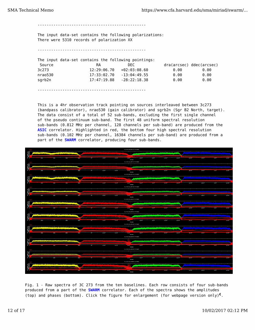
This is a 4hr observation track pointing on sources interleaved between 3c273 (bandpass calibrator), nrao530 (gain calibrator) and sgrb2n (Sgr B2 North, target). The data consist of a total of 52 sub-bands, excluding the first single channel of the pseudo continuum sub-band. The first 48 uniform spectral resolutionsub-bands (0.812 MHz per channel, 128 channels per sub-band) are produced from theASIC correlator. Highlighted in red, the bottom four high spectral resolution sub-bands (0.102 MHz per channel, 16384 channels per sub-band) are produced from a part of the SWARM correlator, producing four sub-bands.

Fig. 1 - Raw spectra of 3C 273 from the ten baselines. Each row consists of four sub-bandsproduced from a part of the SWARM correlator. Each of the spectra shows the amplitudes(top) and phases (bottom). Click the figure for enlargement (for webpage version only)€.


12 of 17 10/02/2017 02:12 PM

Below, using the data extracted for the four high spectral resolution SWARM sub-bands, we demonstrates the process of solving bandpass with smamfcal, showing the results from the Miriad task smamfcal.

Using an SMA pre-process program swarmsplt, we binned every two channels together before solving for bandpass. We note that the current code works for 8192 spectral channels per sub-band or the original spectral data binned every two channels from the full resolution (16384 channels) data due to some issues. Miriad is being upgraded towards a full capacity in handling SWARM data for SMA science.

6.2. Raw spectra of 3C 273 - bandpass calibratorThe beginning of the observation tracks was on 3C 273, bandpass calibrator, for 30 minutes. Fig. 1 shows a set of spectra of the four SWARM sub-bands from 10 baselines. Each SWARM sub-band is marked in different color. 3C 273 at 1.3 mm is a strong point source (~11 Jy). Thus, weighting with visibility variance (default) would be good enough. Using the setup given as an example in Section 5, we run smamfcal to solve for bandpass.

Fig. 2 - Antenna-based solutions in amplitude derived from the bandpass solver smamfcal. Click the figure for enlargement (for webpage version only)€.


13 of 17 10/02/2017 02:12 PM

6.3. Bandpass solutionsThe bandpass solutions are obtained from the solver smamfcal in Miriad. Fig. 2 showsthe antenna-based bandpass solutions in amplitude for the four SWARM sub-bands (colorcoded). We note that 500 channels, or 1000 channels for the data with the original channel resolution, have been cut off from both edges of each sub-band. The sub-band 2 at the large channel series number end may have more low signalchannels that need to be thrown away.

Fig. 3 shows the antenna-based bandpass solutions in phase for the four SWARMsub-bands coded with the same color corresponding to the amplitude solutions. We note that the antenna 1 is used as reference and the rest of antennas show significant phase offsets between the sub-bands while small phase variaitions appear in eachsub-bands. The alignment in phase is critical in continuum imaging. Applyingthe bandpass solutions to the target sources, the instrumental issues are takencare automatically.

Fig. 3 - Antenna-based solutions in phase derived from the bandpass solver smamfcal,corresponding to the solutions in amplitude shown in Fig. 2. Antenna 1 is the reference antenna. Click the figure for enlargement (for webpage version only)€.


14 of 17 10/02/2017 02:12 PM

SWARM sub-band 1 -

SWARM sub-band 2 -


15 of 17 10/02/2017 02:12 PM

SWARM sub-band 3 -

SWARM sub-band 4 -


16 of 17 10/02/2017 02:12 PM

Fig. 4 - A stack of 10 spectra from each baseline in each of the four SWARMsub-bands towards Sgr B2 North after apply corrections for bandpass. From top to bottomare the sub-bands 1, 2, 3 and 4 produced from a part of the SWARM correlator. Click each of the figures for enlargement (for webpage version only)€.

6.4. Spectra of Sgr B2 NorthWe apply the bandpass solutions derived from 3C 273 to the target Sgr B2 North. Fig. 4shows a stack of 10 corrected spectra from each baseline in each of the four SWARMsub-bands. A forest of molecular lines is present in the SWARM spectra; some show abroad absorption (for example, a feature at around 214.2 GHz in SWARM sub-band 1) andsome are associated with very strong emission lines. The hydrogen recombination line H30α is hidden in the line forest of the upper sideband (USB) spectra (not shwon in this Memo).

Finally, we note that the scale of flux density and complex gain corrections have not been applied to the spectra of the target source yet as shown in Fig. 4.

Appendix: Source code -

The Fortran code of the entire smamfcal program exceeds 4600 coding lines. For interested users, a copy of the source code can be found from the SMA Miriad distribution. The codeof the Fortran 77 subroutines for the relevant pre-processes is highlighted below:

accumwt - weightavgchn - vector averagedivchz - normalizationsmoothply - moving smooth & orthogonal polynomial fit

Reference -

[1]Sault, R. J., Teuben, P. J., & Wright, M. C. H. 1995, in ASP Conf. Ser. 77, Astronomical Data Analysis Software and Systems IV, ed. R. A. Shaw, H. E. Payne, & J. J. E. Hayes (San Francisco, CA: ASP), 433[2]Basmah Riaz, 2016, personel communication based on her SMA project: 2015B-S044[3]Long, F. et al. 2017, ApJ, 844, 99[4]Ricci, L. et al. 2012, ApJL, 761, L20[5]Rau, U. & Cornwell, T. J. 2011, AA, 532, A71, for example[6]Jun-Hui Zhao, Mark, R. Morris, & W. M. Goss 2017, in preparation[7]Siegmund Brandt, 1999, Data Analysis - Statistical and Computational Methods for Scientists and Engineers, Third Edition, Springer-Verlag New York Inc.

___________________€https://www.cfa.harvard.edu/sma/miriad/swarm/SMAmemSWARMBpass/SMAmemSWARMBpass.html


17 of 17 10/02/2017 02:12 PM

SMA Technical Memo #166 - · era of wideband SMA. This technical memo reports a progress of Miriad...

Documents

Transcript of SMA Technical Memo #166 - · era of wideband SMA. This technical memo reports a progress of Miriad...