376 Asian Journal of Control, Vol. 6, No. 3, pp. 376-387, September 2004

Manuscript received August 9, 2002; revised November 27,2002; accepted September 4, 2003.

The authors are with Department of Electrical and ControlEngineering, National Chiao Tung University, 1001 Ta HsuehRoad, Hsinchu 30010, Taiwan.

This paper was in part supported by the National ScienceCouncil, Taiwan under Grant No. NSC90-2212-E-009-063.

SLIDING-MODE LINEARIZATION TORQUE CONTROL OF AN INDUCTION MOTOR

Shir-Kuan Lin and Chih-Hsing Fang

ABSTRACT

This paper proposes a sliding-mode linearization torque control (SMLTC) for an induction motor (IM). An ideal feedback linearization torque control method is firstly adopted in order to decouple the torque and flux amplitude of the IM. However, the system parameters are uncertainties, which will influence the control performance of the IM in practical applica-tions. Hence, to increase the robustness of the IM drive for high- perform-ance applications, this SMLTC aims to improve the immunity of those uncertainties. We modify the flux observer of Benchaib and Edwards [15] by means of the adaptive sliding-mode method. This not only eliminates the es-timation of the uncertainty bounds, but also improves the performance of sliding control. In addition, a practical application of the proposed SMLTC, with a model reference adaptive control (MRAC) scheme incorporated as the inner and outer loop controller used for position control, is also presented. Some experiments are presented to verify the control theory and demonstrate the robustness and effectiveness of the proposed SMLTC.

KeyWords: Induction motor (IM), sliding-mode linearization torque con-trol (SMLTC), adaptive sliding-mode observer, model refer-ence adaptive control (MRAC).

I. INTRODUCTION

Induction motors (IM) have been widely applied in various industries because of their advantages of simple construction, ruggedness, reliability, low cost, and minimum maintenance. A new challenge is to use in-duction motors in precision servo machines, such as robots and NC machines. However, a problem arises from the load variation that occurs as the motor operates. The computed-torque control was proposed to solve such a position tracking problem for robots [1].

Torque control has been widely used as the inner loop controller to solve the speed and/or position track-ing problems of an induction motor. In recent decades, many concepts of torque control have been proposed.

Field-orientated control (FOC) for induction motor drives [2-5] provides decoupling control between the torque and flux components, and is able to obtain good performance, similar to that of a DC motor. However, it was shown in [5] that the FOC is not robust to parame-ter variation. Direct torque control (DTC) is another strategy that has received attention in the recent years [6-8]. The basic idea behind DTC is to directly select the stator voltage vector according to the differences between the references of the torque and stator flux and their actual values [6]. The advantages of DTC are quick torque response and less parameter dependence, but chattering is its drawback. To eliminate chattering, feedback linearization control has been successfully applied to induction motor torque control [9,10]. How-ever, it requires precise values of the system parameters.

In the last decade, the variable structure control strategy using the sliding-mode has been the focus of many studies and research on the control of the AC drive system [11-15]. The key objective of this tech-nique is to force the system trajectory to a specific sur-face, known as the sliding surface, such that the state

S.K. Lin and C.H. Fang: Sliding-Mode Linearization Torque Control of an Induction Motor 377

variables of the system are totally determined by the sliding surface. The main feature of the approach is its insensitivity to disturbances and parameter variations.

This paper presents a new sliding-mode lineariza-tion torque control (SMLTC) for an induction motor. The torque control is established by designing two slid-ing surfaces for the torque and flux, respectively. The sliding surface for the torque is based on the inte-gral-sliding surface, whereas the sliding surface for the flux is based on that of Benchaib et al., [14]. In common, the linearization controller can be designed if the deriva-tive of the surface function is established while the pa-rameters are known. Actually, the IM exhibits uncertainties of the plant, such as electrical parameter variations and external disturbance in practical applica-tions. Designing a linearization controller that is insen-sitive to those parameters under application of the sliding surface concept is our objective. Thus, a sliding- mode linearization torque controller is proposed to de-couple the torque and flux amplitude the IM drive. The control laws of the sliding- mode linearization torque control are derived from the sense of the Lyapunov sta-bility theorem, such that asymptotic stability of the con-trol system can be guaranteed under the occurrence of system uncertainties. To obtain the amplitudes of the torque and flux, a rotor flux observer is needed. Ben-chaib and Edwards [15] proposed a robust flux observer, which can accurately estimate the stator current regard-less the flux error and then estimate the rotor flux using the estimated current. In this paper, we modify this flux observer by incorporating the adaptive sliding-mode method. This not only eliminates estimation of the un-certainty bounds but also improves the performance of sliding-mode control. Finally, we apply this sliding- mode linearization torque controller to the position con-trol of an induction motor. The sliding-mode lineariza-tion torque control is the inner loop controller, while a model reference adaptive control (MRAC) scheme for the position control is used as the outer loop controller. The mechanical system of an IM with a rod fixed on the shaft is considered as an experimental system to verify the effectiveness and applicability of this proposed SMLTC.

This paper is organized as follows. Section 2 re-views the model of the IM. The proposed SMLTC and the flux observer are presented in section 3. Section 4 addresses the application to the position control and gives experimental results. Finally, section 5 draws con-clusions.

II. MODEL OF AN INDUCTION MOTOR

Let Rs and Rr be the stator and rotor resistance, re-spectively; let Ls, Lr, and M be the stator, rotor, and mu-

tual inductance, respectively; let B and J be the friction coefficient and the moment of inertial of the motor, re-spectively; and let p be the number of pole-pairs. Fur-thermore, define Tr = Lr / Rr as the rotor time constant. Then, the mathematical model of an induction motor in a stator-fixed frame (α, β) can be described by five nonlinear differential equations with four electrical variables [stator currents (iαs, iβs) and rotor fluxes (ϕαr, ϕβr)], a mechanical variable [rotor speed (ωm)], and two control variables [stator voltages (uαs, uβs)] [2,16] as follows:

s s r m r sr

Ki i pK uT

= − + + +α α α β αγ ϕ ω ϕ α (1)

s s r m r sr

Ki i pK uT

= − + − +β β β α βγ ϕ ω ϕ α (2)

1r s r m r

r r

M i pT T

= − −α α α βϕ ϕ ω ϕ (3)

1r s r m r

r r

M i pT T

= − +β β β αϕ ϕ ω ϕ (4)

e Lm m

T TBJ J J

= − + −ω ω (5)

where Te and TL are the electromagnetic torque and ex-ternal load torque. Note that

( )e T s r s rT k i i= −β α α βϕ ϕ (6)

and that the parameters used in (1)-(5) are defined as σ ≡ 1 – M

2/(Ls Lr), K ≡ M/(σLs Lr), α ≡ 1/(σLs), γ ≡ Rs /(σLs) + Rr M

2/(σLs Lr2), and kT ≡ (3p/4)(M/Lr).

III. CONTROL SCHEME

3.1 Sliding-mode linearization torque control

The SMLTC scheme is designed to control the electromagnetic torque Te to track the desired one by means of voltage inputs. It is well known that the squared norm of the rotor fluxes plays an important role in the performance of a motor and is also closely related to the electromagnetic torque. We then want to control the active torque uT and the square of the flux norm uφ = φ2, which are defined as

T s r s ru i i= −β α α βϕ ϕ (7)

2 2r ru = +φ α βϕ ϕ (8)

378 Asian Journal of Control, Vol. 6, No. 3, September 2004

Define the errors as eT ≡ uT – uTref and eφ ≡ uφ − uφ ref, where uTref and uφ ref are the reference values of the active torque and the square of the flux norm, respectively.

The sliding-mode control is first used to find the sliding surface s = 0, such that the errors eT and eφ on this surface approach zero as time approaches infinity. In the present case, we define s = [s1 s2]T. We adopt the integral and the differential surface functions for the active torque and the square of the flux norm, respec-tively, to obtain

1 1 0(0 )

tT T Ts e k e dt e −⎛ ⎞= + −⎜ ⎟

⎝ ⎠∫ (9)

2 2 22 [ ( ) ]as ar bs br refr

ds e k e k e M i i u udt T

= + = + + − −φ φ φ φ φϕ ϕ

(10)

where k1 and k2 are positive gains. If the system remains stationary on the surface, then 02121 ==== ssss . Substituting (9) and (10) into 01 =s and 02 =s yields

1( ) ( )T Tref T Trefd u u k u udt

− = − − (11)

2( ) ( )ref refd u u k u udt

− = − −φ φ φ φ (12)

Equations (11) and (12) ensure that the system states (uT and uφ) will exponentially converge to the reference values if they are kept on the sliding surfaces, s = 0.

The next mission is to design the switching input u = [uαs uβs]T for (1) and (2) that will drive the state vari-ables of the system to the sliding surface, s = 0, and keep them there. We select the Lyapunov function [17] candidate as

12

TV = s s (13)

The time derivative of V requires the derivatives of s. Substituting (1)-(4) into the derivatives of (9) and (10), we obtain the dynamical equations of the switching sur-face variables as

1 1T Ts e k e= +

11 ( )T m dr

k u p KuT φγ ω φ

⎛ ⎞= − − − +⎜ ⎟

⎝ ⎠

1 Tref Tref r s r sk u u u u− − + −α β β ααϕ αϕ (14)

2 2 ( )refs k u uφ φ= −

2 [ ( ) ]s r s r s r s r refr

M i i i i u uT α β α α β α β α φ φϕ ϕ ϕ ϕ+ + + + − −

⎢⎢⎣

⎡φ⎟⎟

⎠

⎞⎜⎜⎝

⎛γ+−+⎟⎟

⎠

⎞⎜⎜⎝

⎛−= φ d

r

i

rrr Tm

TM

TMu

Tk 122

2

2m T ref refr

K u p u k u uT φ φ φω

⎤+ + − −⎥

⎦

2 ( )r s r sr

M u uT

+ +α α β βαϕ αϕ (15)

or

Dubs += (16)

where Tbb ][ 21=b

2 2

r r

r rr r

M MT T

β α

α β

αϕ αϕ

α ϕ α ϕ

−⎡ ⎤⎢ ⎥= ⎢ ⎥⎢ ⎥⎣ ⎦

D (17)

in which

1 1 11 ( )T m d Tref Trefr

b k u p Ku k u uT φγ ω φ

⎛ ⎞= − − − + − −⎜ ⎟

⎝ ⎠

2 22 2 1

i dr r r r

M Mb k u mT T T Tφ γ φ

⎡⎛ ⎞ ⎛ ⎞= − + − +⎢⎜ ⎟ ⎜ ⎟

⎢⎝ ⎠ ⎝ ⎠⎣

2m T ref refr

K u p u k u uT φ φ φω

⎤+ + − −⎥

⎦

d s r s ri iα α β βφ ϕ ϕ= +

2 2i s sm i iα β= +

Under the assumption that the parameters are known a priori, it can be shown that s1 and s2 converge to zero as t → ∞ if the following linearization controller is applied:

1( )ck−= − +u D b s (18)

where kc is a control gain and the inverse D−1 exists at all times.

However, the system parameters (e.g., Rs, Rr, Ls, Lr, M) in (1)-(4) are uncertainties and include external dis-turbance noise, n, so (16) should be modified as

= + ∆ + + ∆ +s (b b) (D D) u n = + + + ∆b Du z Dn (19)

where ∆b and ∆D are the uncertainties induced by the model uncertainties in (1)-(4) and

nbz +∆= (20)

Proposition 1. Consider the induction motor in (1)-(4). Suppose that [z1

* z2*]T are the upper bounds of the com-

ponents of the uncertainty z in (20), and that 1 2[ ]Tξ ξ ,

S.K. Lin and C.H. Fang: Sliding-Mode Linearization Torque Control of an Induction Motor 379

1 2[ ]Tξ ξ , and 1 2

3 4

δ δδ δ

⎡ ⎤⎢ ⎥⎣ ⎦

are, respectively, the upper

bounds of the components of the uncertainties ∆DD−1b, ∆DD−1s, and ∆DD−1, respectively. Furthermore, assume that 1 − δ1 − δ4 + δ1δ4 − δ2δ3 > 0, 1 > δ1, and 1 > δ4. If the controller is designed so that the stator voltages are

ick usbDu ++−= − )(1 (21)

1 11

2 2

sign( )sign( )

ci

c

ss

µµ

− ⎡ ⎤= − ⎢ ⎥

⎣ ⎦u D (22)

then the overall system will asymptotically converge to T Trefu u= and refu uφ φ= , provided that the inverse

D−1 exists at all times, and that 1 *

1 1 2 1 1 1*

2 3 4 2 2 2

11

c c

c c

z k

z k

µ δ δ ξ ξµ δ δ ξ ξ

− ⎡ ⎤− − + +⎡ ⎤ ⎡ ⎤≥ ⎢ ⎥⎢ ⎥ ⎢ ⎥− − + +⎣ ⎦ ⎣ ⎦ ⎢ ⎥⎣ ⎦

(23)

Note that

)( 111ic

TT k uDDsDDbDDsDus −−− ∆+∆+∆−=∆

1 1 1 1 2 2 1( ) | |c c ck sξ ξ δ µ δ µ≤ + + +

2 2 3 1 4 2 2( ) | |c c ck sξ ξ δ µ δ µ+ + + + (24)

Proof. The Lyapunov candidate function V in (13) is positive definite and radially unbounded. Substituting (19) into (16) and using (24), we obtain

TV = s s

1 1

2 2

sign( )sign( )

cT Tc

c

sk

sµµ

⎛ ⎞⎡ ⎤= − − − + + ∆⎜ ⎟⎢ ⎥

⎣ ⎦⎝ ⎠s b b s z s Du

* *1 1 2 2 1 1 2 2| | | | | | | |T

c c ck s s z s z sµ µ≤ − − − + +s s

1 1 1 1 2 2 1( ) | |c c ck sξ ξ δ µ δ µ+ + + +

2 2 3 1 4 2 2( ) | |c c ck sξ ξ δ µ δ µ+ + + + *

1 1 2 2 1 1 1 1[(1 ) ( )] | |Tc c c ck z k sδ µ δ µ ξ ξ= − − − − − + +s s

*3 1 4 2 2 2 2 2[ (1 ) ( )] | |c c cz k sδ µ δ µ ξ ξ− − + − − + +

Tck≤ − s s (25)

which is negative definite. The last inequality follows from (23). It should be noted that (23) implies that µc1 ≥ 0 and µc2 ≥ 0 because of the assumptions of 1 − δ1 − δ4 + δ1δ4 − δ2δ3 > 0, 1 > δ1, and 1 > δ4. According to Lyapunov’s theory, s = 0 is globally asymptotically sta-ble. Any value of s will converge to zero, and it was pointed out earlier that the active torque uT and the square of the flux norm uφ will converge to the reference values if s = 0 holds permanently. This completes the proof.

Remark 1. The restriction of the existence of the in-verse D−1 is easily satisfied. According to (17), D is nonsingular if and only if uφ is nonzero. The constraint uφ > 0 will be satisfied if the initial value is greater than zero. Nevertheless, in the implementation, uφ is replaced with a small value of δφ > 0 if uφ < δφ.

The undesirable chattering of sliding-mode tech-niques can be remedied by replacing the switching func-tion sign(si) with the saturation function of

1 if

Sat( ) if | |

1 if

i

ii i

i

ss

s s

s

λ

λλ

λ

>⎧⎪⎪= ≤⎨⎪

− < −⎪⎩

(26)

where λ > 0 represents the thickness of the boundary layer.

Remark 2. It is possible to estimate the upper bounds of the components of the uncertainties ∆DD−1b, ∆DD−1s, and ∆DD−1, when the upper bounds of z, (z1

*, z2*), and

those of the components of ∆D are given. In a simula-tion, we first let µc1 ≥ z1

* and µc2 ≥ z2*, and then obtain

the histories of ∆DD−1b, ∆DD−1s, and ∆DD−1 by means of simulation, which provide the estimates of the upper bounds. Usually, it is best to multiply the upper bounds in the histories by a factor, say 20%, to obtain the esti-mates. On the other hand, the assumptions of 1 − δ1 − δ4

+ δ1δ4 − δ2δ3 > 0, 1 > δ1, and 1 > δ4 can be satisfied when the bounds of ∆D are sufficiently small. As a nu-merical example, the same motor used in the experi-ments described in section 4.2 was used to perform a simulation. The uncertainties of Rs, Rr, Ls, Lr, M were all 50% of the nominal values. The history of ∆DD−1 was calculated, from which it was found that δ1 ∈ (0, 0.36), δ2 ∈ (0, 0.05), δ3 ∈ (−0.001, 0.001), and δ4 ∈ (−0.001, 0.001). This also indicates that 1 − δ1 − δ4 + δ1δ4 − δ2δ3 > 0 is always satisfied.

3.2 Adaptive sliding-mode observer

The above sliding-mode linearization torque control requires the signals of uφ , iαs and iβs. The currents iαs and iβs can be measured. However, uφ is difficult to obtain. A flux observer is, then, necessary. According to the model in (1)-(4), the flux observer is proposed as

1ˆ ˆ ˆ ˆs s r m r s

r

Ki i pK uTα α α β αγ ϕ ω ϕ α= − + + + + Λ (27)

2ˆ ˆ ˆ ˆs s r m r s

r

Ki i pK uTβ β β α βγ ϕ ω ϕ α= − + − + + Λ (28)

31ˆˆ ˆ ˆr s r m r

r r

M i pT Tα α α βϕ ϕ ω ϕ= − − + Λ (29)

380 Asian Journal of Control, Vol. 6, No. 3, September 2004

41ˆˆ ˆ ˆr s r m r

r r

M i pT Tβ β β αϕ ϕ ω ϕ= − + + Λ (30)

where ˆ ,siα ˆ ,siβ ˆ ,rαϕ and ˆ rβϕ are the estimates of ,siα ,siβ ,rαϕ and rβϕ , respectively. Λi, i = 1, …, 4,

are the observer inputs to be designed. The estimate errors are

1

2

3

4

ˆˆ

ˆˆ

s s

s s

r r

r r

i iei ie

ee

α α

β β

α α

β β

ϕ ϕϕ ϕ

⎡ ⎤−⎡ ⎤⎢ ⎥⎢ ⎥ −⎢ ⎥⎢ ⎥= = ⎢ ⎥⎢ ⎥ −⎢ ⎥⎢ ⎥⎢ ⎥−⎣ ⎦ ⎣ ⎦

e (31)

It follows from (27)-(30) that

1 1 1 1 1e eγ ζ= − + + ∆ + Λ (32)

2 2 2 2 2e eγ ζ= − + + ∆ + Λ (33)

3 3 4 1 3 31

mr r

Me e p e eT T

ω= − − + + ∆ + Λ (34)

4 4 3 2 4 41

mr r

Me e p e eT T

ω= − + + + ∆ + Λ (35)

where ∆1, ∆2, ∆3, and ∆4 are uncertainties, and

1 3

2 4

mr

mr

K pKTζ e

ζ eKpKT

ω

ω

⎡ ⎤⎢ ⎥⎡ ⎤ ⎡ ⎤⎢ ⎥= ≡⎢ ⎥ ⎢ ⎥⎢ ⎥⎣ ⎦ ⎣ ⎦−⎢ ⎥⎣ ⎦

ζ (36)

It should be remarked that ∆1 and ∆2 are bounded only if uαs and uβs are bounded, and the uncertainty ∆α of α is also bounded, since ∆1 includes ∆αuαs and ∆2 includes ∆αuβs.

We will briefly review the sliding-mode flux ob-server proposed by Benchaib and Edward [15]. They designed a sliding-mode controller for the first two equations of the flux observer, i.e., (27) and (28). This sliding-mode scheme forces the estimates ˆ

siα and ˆsiβ

to converge to the measured currents iαs and iβs regard-less of the errors of the flux estimates e3 and e4. The sliding-mode inputs proposed by Benchaib and Edwards are [15]

1 1 1

2 2 2

sign( )

sign( )

e

e

Λ = −⎧⎪⎨

Λ = −⎪⎩

ρ

ρ (37)

with the following chosen sliding gains ρ1 and ρ2:

1 1 1 2

2 2 2 1

ˆ ˆ| | ( | |) | | ( | |)

ˆ ˆ| | ( | |) | | ( | |)

ar m brr

br m arr

Ke pKTKe pKT

ρ γ η ϕ ω η ϕ

ρ γ η ϕ ω η ϕ

⎧ > + + + +⎪⎪⎨⎪ > + + + +⎪⎩

(38)

where η1 and η2 are the upper bounds of |ϕαr| and |ϕβr|, respectively. As e1 and e2 are zero, (32) and (33) make e3 and e4 rely on Λ1 and Λ2, solely which can be used to stabilize (34) and (35). However, ρ1 and ρ2 are always large so that the chattering phenomenon is still a serious problem. A remedy is to use the adaptive sliding-mode technique.

We suppose that ζ in (36) varies around a nominal constant value ζ

*. Then, (32), and (33) can be rewritten as

* *1 1 1 1 1e e ζγ= − + + ∆ + Λ (39)

* *2 2 2 2 2e e ζγ= − + + ∆ + Λ (40)

where ∆i * = ζi − ζi

* + ∆i, i = 1, 2. If the inputs are de-signed as

*1 1 1 1

*2 2 2 2

sign( )

sign( )

e ζ

e ζ

⎧ Λ = − −⎪⎨

Λ = − −⎪⎩

ρ

ρ (41)

with ρ1 > | ∆1*| and ρ2 > | ∆1

*| for all t, then it can be shown by means of the sliding-mode theory that e1 and e2 converge to zero as t → ∞.

However, ζ1* and ζ2

*, and the upper bounds of |∆1*|

and |∆2*|, are unknown. We then need the following

adaptive sliding-mode observer inputs:

1 1 1 1

2 2 2 2

ˆˆ sign( )

ˆˆ sign( )

e ζ

e ζ

⎧ Λ = − −⎪⎨⎪Λ = − −⎩

ρ

ρ (42)

where ˆ iρ and ˆiζ are, respectively, the estimates of

ρi and ζi *, i = 1, 2.

Lemma 2. The current estimator in (27) and (28) with the inputs of (42) ensures that e1 and e2 converge to zero if e3 and e4 are bounded and the adaptive laws are

1 1

22

ˆ | |ˆ

| |ˆ

ee

ρ

ρ

⎡ ⎤ ⎡ ⎤= = =⎢ ⎥ ⎢ ⎥

⎢ ⎥ ⎣ ⎦⎣ ⎦ρ ρ (43)

1 1

22

ˆˆ

ˆ

ζ eeζ

⎡ ⎤ ⎡ ⎤⎢ ⎥= = = ⎢ ⎥⎢ ⎥ ⎣ ⎦⎣ ⎦ζ ζ (44)

Proof. Let the sliding surface function be so1 = [e1 e2]T.

S.K. Lin and C.H. Fang: Sliding-Mode Linearization Torque Control of an Induction Motor 381

Define the Lyapunov-like function as

2 2 21

1 ( )2o oV = + +s ρ ζ (45)

where ˆ= −ρ ρ ρ and *ˆ= −ζ ζ ζ . It follows from (39), (40), and (42) that

1 1 T T To o oV = + +s s ρ ρ ζ ζ

1 1*1 1 1

2 2

ˆ sign( )( )

ˆ sign( )T To o o

e

e

ργ

ρ

⎛ ⎞⎡ ⎤⎜ ⎟= − + + − ⎢ ⎥⎜ ⎟⎢ ⎥⎣ ⎦⎝ ⎠

s s ζ s ∆

1 11 1

2 2

ˆ sign( )ˆ sign( )

T T To o

e

e

ργ

ρ

⎛ ⎞⎡ ⎤⎜ ⎟+ + ≤ − + + ⎢ ⎥⎜ ⎟⎢ ⎥⎣ ⎦⎝ ⎠

ρ ρ ζ ζ s s ζ

1 1 0T T To oγ+ + = − ≤ρ ρ ζ ζ s s (46)

The last equality in (46) is obtained by applying the adaptive laws (43) and (44). Note that [ρ1sign(e1), ρ2sign(e2)] so1 ≥ *

1Tos ∆ .

The fact that Vo is bounded below and nonincreas-ing implies that lim t → ∞ Vo = Vo∞ exists [17]. Thus, so1,

, ,L∞∈ρ ζ which implies that ˆˆ ,L∞∈ρ, ζ since ρ and *ζ are constants. It then follows from (39), (40), and

(42) that 1o L∞∈s . Integrating (46), we obtain Vo0 −

Vo∞ 1 10

To o dt

∞≥ γ∫ s s and then 1 2o L∈s . A corollary of

Barbalat’s lemma [17] states that 1o L∞∈s and

1 2o L∈s imply that so1 → 0 as t → ∞. This completes

the proof.

Proposition 3. The flux observer (27)-(30) ensures that the flux estimate errors e3 and e4 converge to zero if we apply the adaptive sliding-mode scheme: (42)-(44) and

1

3 1

4 2

mm r

mm

r

K pKk p T

p k KpKT

φ

φ

ωω

ωω

−⎡ ⎤⎢ ⎥−Λ Λ⎡ ⎤⎡ ⎤ ⎡ ⎤⎢ ⎥= ⎢ ⎥⎢ ⎥ ⎢ ⎥⎢ ⎥Λ Λ⎣ ⎦ ⎣ ⎦⎣ ⎦ −⎢ ⎥⎣ ⎦

3 3

4 4

sign( )sign( )

ee

ρρ

⎡ ⎤− ⎢ ⎥

⎣ ⎦ (47)

where kφ > 0 is a constant observer gain; [ρ3 ρ4]T represents the upper bound of the uncertainty of the estimated flux equations.

Proof. According to Lemma 2, when t is sufficiently large, we have so1 = 1os = 0, which, by combining (32),

(33), and (36), yields 1

1 1 3

2 2 4

mr

mr

K pKT e

eKpKT

ω

ω

−⎡ ⎤⎢ ⎥ Λ + ∆⎡ ⎤ ⎡ ⎤⎢ ⎥ = −⎢ ⎥ ⎢ ⎥⎢ ⎥ Λ + ∆⎣ ⎦ ⎣ ⎦−⎢ ⎥⎣ ⎦

(48)

By (48), we can rewrite (47) as

3 3 3 3

4 4 4 4

sign( )sign( )

m

m

k p e ep k e e

φ

φ

ω ρω ρ

−Λ ⎡ ⎤⎡ ⎤ ⎡ ⎤ ⎡ ⎤= − −⎢ ⎥⎢ ⎥ ⎢ ⎥ ⎢ ⎥Λ⎣ ⎦ ⎣ ⎦ ⎣ ⎦⎣ ⎦

1

1

2

mm r

mm

r

K pKk p T

p k KpKT

φ

φ

ωω

ωω

−⎡ ⎤⎢ ⎥− ∆⎡ ⎤ ⎡ ⎤⎢ ⎥− ⎢ ⎥ ⎢ ⎥⎢ ⎥ ∆⎣ ⎦⎣ ⎦ −⎢ ⎥⎣ ⎦

(49)

Substituting (49) into (34) and (35), we obtain

3 3

4 4

1 0

10

r

r

kTe e

e ekT

φ

φ

⎡ ⎤− −⎢ ⎥⎡ ⎤ ⎡ ⎤⎢ ⎥=⎢ ⎥ ⎢ ⎥⎢ ⎥⎣ ⎦ ⎣ ⎦− −⎢ ⎥⎣ ⎦

*3 3 3

*4 4 4

sign( )sign( )

ee

ρρ

⎡ ⎤∆⎡ ⎤− + ⎢ ⎥⎢ ⎥

∆⎣ ⎦ ⎢ ⎥⎣ ⎦ (50)

where 1

*3 1 3*

2 44

mm r

mm

r

K pKk p T

p k KpKT

φ

φ

ωω

ωω

−⎡ ⎤⎢ ⎥⎡ ⎤ −∆ ∆ ∆⎡ ⎤ ⎡ ⎤ ⎡ ⎤⎢ ⎥= +⎢ ⎥ ⎢ ⎥ ⎢ ⎥ ⎢ ⎥⎢ ⎥ ∆ ∆∆ ⎣ ⎦ ⎣ ⎦⎢ ⎥ ⎣ ⎦⎣ ⎦ −⎢ ⎥⎣ ⎦

(51)

Define the sliding surface function so2 = [e3 e4]T. Then, a standard proof process will show that the system finally converges to the sliding surface so2 = 0. This means that e3 and e4 approach zero as t → ∞.

Remark 3. To reduce the amount of chattering, we can still replace the switching function sign(ei) in (42) and (47) with the saturation function of

1 if

Sat( ) if | |

1 if

i

ii i

i

ss

s s

s

λ

λλ

λ

>⎧⎪⎪= ≤⎨⎪

− < −⎪⎩

(52)

where λ > 0 represents the thickness of the boundary layer. On the other hand, it should be emphasized that the uncertainties have also been taken into account in the observer design, i.e., ∆1, ∆2, ∆3, and ∆4 in (32) to (35).

382 Asian Journal of Control, Vol. 6, No. 3, September 2004

IV. APPLICATION TO POSITION CONTROL

4.1 Model reference adaptive control

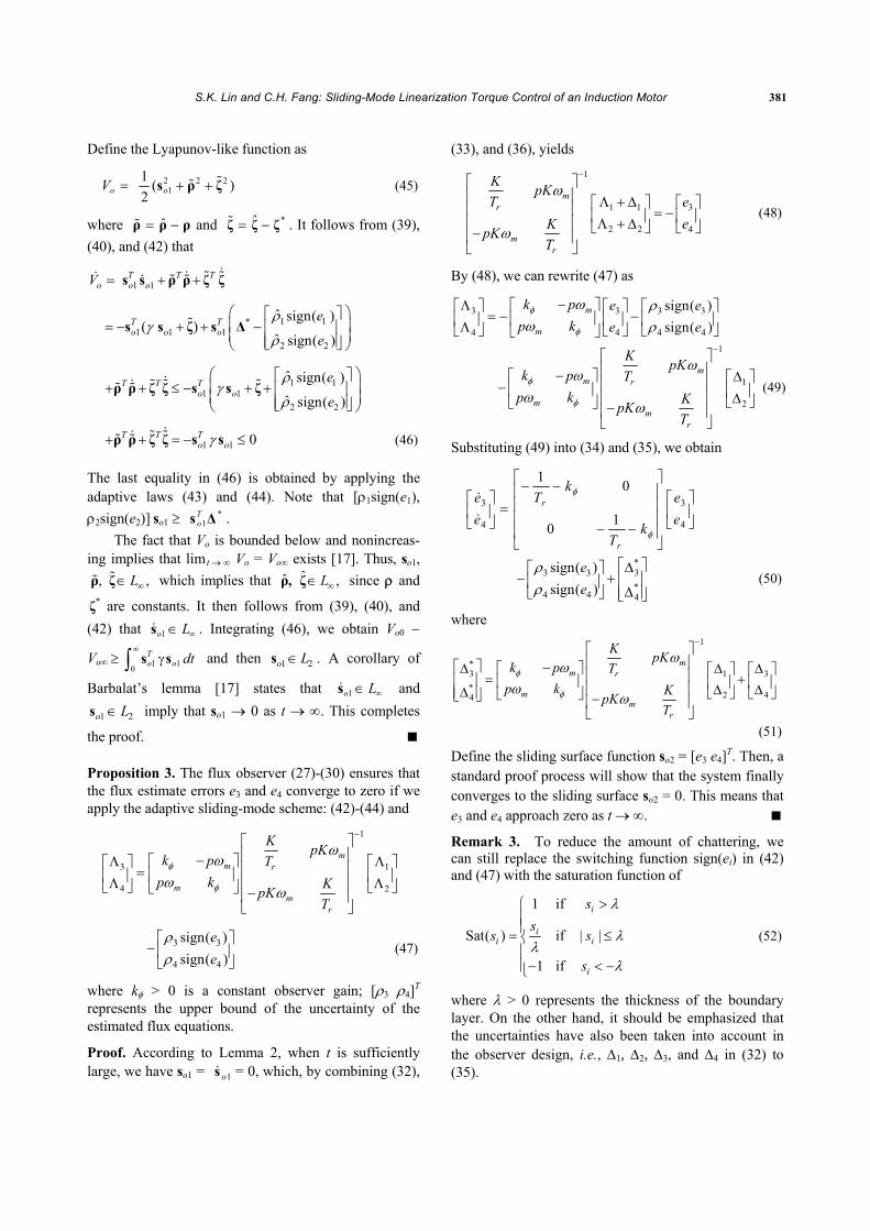
We want to apply the above sliding-mode linearization torque control to the position control of a mechanical system driven by an induction motor. The block diagram in Fig. 1 illustrates the overall system of the proposed control method. The inner loop controller is the sliding-mode linearization torque control, and it consists of the torque/flux control and observer, while a model reference adaptive control scheme will be used as the outer loop position controller. The position controller generates the torque command for the inner loop controller, which then asks the inverter to provide the required three-phase voltages for the induction motor.

The mechanical system to be considered is an induction motor with a rod fixed on the shaft axis of the motor , as shown in Fig. 2. The mechanical model of the system is

0sin( )m m m T TJ B mgl k uθ θ θ θ= − − + +

0 0cos sin sin cosm m m T TB mgl mgl k uθ θ θ θ θ= − − − + (53)

where θm is the angular displacement of the shaft, m is the mass of the rod, l is the distance from the shaft center to the center of the mass of the rod, g is the gravitational acceleration, kT is the torque constant, and θ0 is the null angle from the line of gravity.

Equation (53) can be rewritten as

( sin cos )m J m b m c m J TB L L K uθ θ θ θ= − − + + (54)

where BJ = B/J, Lb = mglsinθ0/J, Lc = mglcosθ0/J, and KJ = kT /J. Note that J > 0.

The model reference adaptive control (MRAC) is one of most popular adaptive control strategies. Since we are concerned with position control, the reference model is given as

* * * * *( )m t m s m s t m s mk k k r k k rθ θ θ θ θ= − − + = − − − (55)

where r is a constant angular displacement, and kt and ks are selected such that s2 + kt s + ks = (s + p1) (s + p2) with p1, p2 > 0.

If we know the system parameters, then the model reference control (MRC) law

*3*2*1*0

sincos

T

m

TmT

m

m

c

cu

crc

θθθθ

⎡ ⎤ ⎡ ⎤⎢ ⎥ ⎢ ⎥⎢ ⎥ ⎢ ⎥= ≡⎢ ⎥ ⎢ ⎥⎢ ⎥ ⎢ ⎥⎢ ⎥ −⎢ ⎥⎣ ⎦⎣ ⎦

*c w (56)

MRACPosition

Controller

IM

Inverter

abci

Vdc

asuSliding-ModeLinearizingTorque/FluxController

bsu

Torque/Flux

Observer

bsas ϕϕ ,

sisu

32 ←

Encoder

φe

Te

φuTu

refu φ

Trefu

−

−+

+

mθ

r

s mω

Fig. 1. Overall system of the position control of an induction

motor.

x

y

LTmθ ml

Fig. 2. Mechanical system of a motor with a rod fixed on the

shaft.

*3*2*1*0

sincos

T

m

TmT

m

m

c

cu

crc

θθθθ

⎡ ⎤ ⎡ ⎤⎢ ⎥ ⎢ ⎥⎢ ⎥ ⎢ ⎥= ≡⎢ ⎥ ⎢ ⎥⎢ ⎥ ⎢ ⎥⎢ ⎥ −⎢ ⎥⎣ ⎦⎣ ⎦

*c w (56)

with *3*2*1*0

( )J t J

b J

c J

s J

c B k Kc L K

L Kck Kc

⎡ ⎤ −⎡ ⎤⎢ ⎥ ⎢ ⎥⎢ ⎥ ⎢ ⎥= =⎢ ⎥ ⎢ ⎥⎢ ⎥ ⎢ ⎥⎢ ⎥ ⎣ ⎦⎣ ⎦

*c (57)

can make the overall system asymptotically track the reference model. However, we do not know the exact values of the system parameters, so we propose the following MRAC:

ˆ ˆT TTu = +c w c w (58)

with

1 , (0)p= − + =w w w w 0 (59)

and the adaptive laws

*ˆ sign( )e ρ= −c Γ w (60)

S.K. Lin and C.H. Fang: Sliding-Mode Linearization Torque Control of an Induction Motor 383

where e = θm −θ*m is the position error, ρ* = KJ /ks, and Γ

is a diagonal matrix with positive diagonal entries. It should be remarked that the sign of ρ* is always known. These adaptive laws actually follow from Table 6.2 in [18], based on the bilinear parametric model

*

1( ) TT

mu

e W ss p

ρ⎛ ⎞

= ⎜ ⎟+⎝ ⎠*c w (61)

where Wm(s) = ks / (s + p2).

4.2 Experiments The overall position control scheme shown in Fig. 1

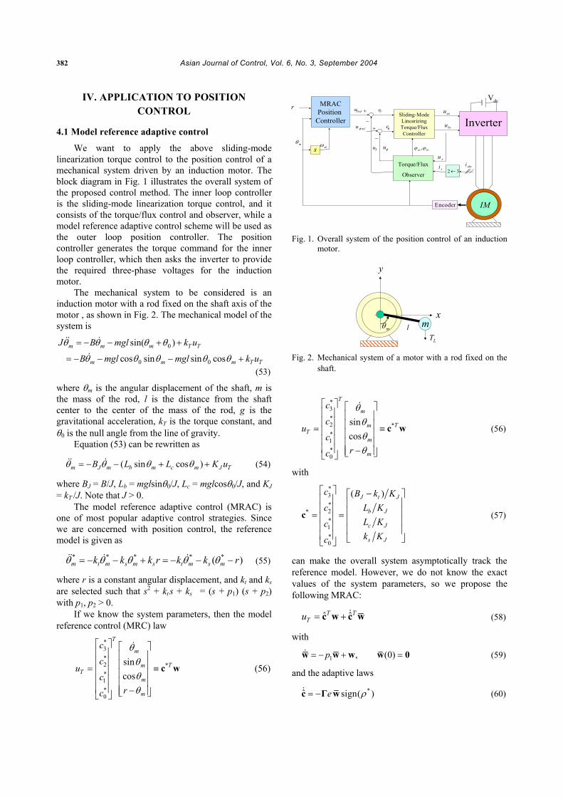
was verified by means of experiments. The experimental system, shown in Fig. 3, was a PC-based control system. A servo control card on the ISA bus of the PC provided eight A/D converters, four D/A converters, and an en-coder counter. The sampling time for overall control was 0.3ms. The ramp comparison modulation circuit was used to generate the PWM to drive the IGBT mod-ule inverter. The induction motor in the experiment sys-tem was a 4-pole, 5HP, 220V motor with a rated current, speed, and torque of 13.4A, 1730rpm, and 18Nm, re-spectively. The encoder had 4096 counters per revolu-tion. The modeling parameters of the motor were Rs = 0.3Ω, Rr = 0.36Ω, Ls = Lr = 48mH, and M = 45mH. Those of the mechanical system (cf. Fig. 1) were J ≈ 0.0069kgm2, l ≈ 0.45m, and m ≈ 3kg. In the following experiments, the gain in the controller (21) was kc = 10, and that in the observer (47) was kφ = 120, so that the response of the observer was much faster than that of the controller.

Three experiments are reported in the following: they focused on (1) torque tracking control, (2) set point position control, and (3) position tracking control, re-spectively. The gains of the reference model (53) were kt = 20 and ks = 100. The popular field-orientated control (FOC) scheme was also applied for the purpose of comparison.

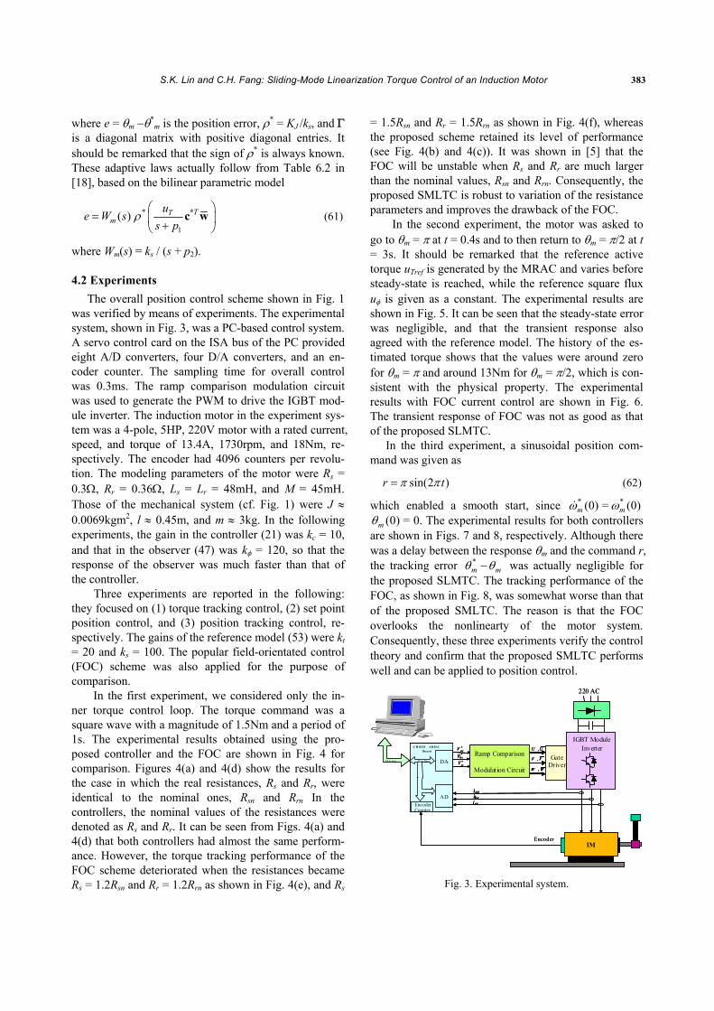
In the first experiment, we considered only the in-ner torque control loop. The torque command was a square wave with a magnitude of 1.5Nm and a period of 1s. The experimental results obtained using the pro-posed controller and the FOC are shown in Fig. 4 for comparison. Figures 4(a) and 4(d) show the results for the case in which the real resistances, Rs and Rr, were identical to the nominal ones, Rsn and Rrn In the controllers, the nominal values of the resistances were denoted as Rs and Rr. It can be seen from Figs. 4(a) and 4(d) that both controllers had almost the same perform-ance. However, the torque tracking performance of the FOC scheme deteriorated when the resistances became Rs = 1.2Rsn and Rr = 1.2Rrn as shown in Fig. 4(e), and Rs

= 1.5Rsn and Rr = 1.5Rrn as shown in Fig. 4(f), whereas the proposed scheme retained its level of performance (see Fig. 4(b) and 4(c)). It was shown in [5] that the FOC will be unstable when Rs and Rr are much larger than the nominal values, Rsn and Rrn. Consequently, the proposed SMLTC is robust to variation of the resistance parameters and improves the drawback of the FOC.

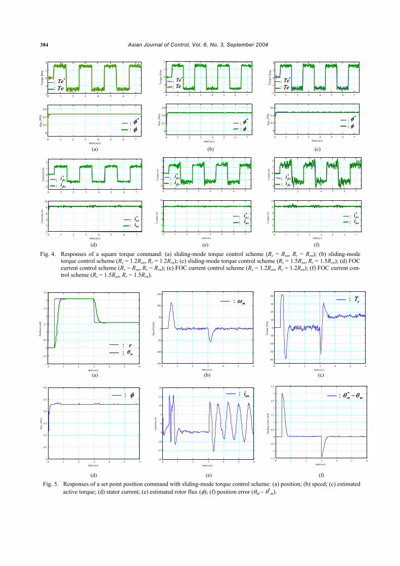
In the second experiment, the motor was asked to go to θm = π at t = 0.4s and to then return to θm = π/2 at t = 3s. It should be remarked that the reference active torque uTref is generated by the MRAC and varies before steady-state is reached, while the reference square flux uφ is given as a constant. The experimental results are shown in Fig. 5. It can be seen that the steady-state error was negligible, and that the transient response also agreed with the reference model. The history of the es-timated torque shows that the values were around zero for θm = π and around 13Nm for θm = π/2, which is con-sistent with the physical property. The experimental results with FOC current control are shown in Fig. 6. The transient response of FOC was not as good as that of the proposed SLMTC.

In the third experiment, a sinusoidal position com-mand was given as

sin(2 )r tπ π= (62)

which enabled a smooth start, since * (0)mω = * (0)mω (0)mθ = 0. The experimental results for both controllers

are shown in Figs. 7 and 8, respectively. Although there was a delay between the response θm and the command r, the tracking error *

m mθ θ− was actually negligible for the proposed SLMTC. The tracking performance of the FOC, as shown in Fig. 8, was somewhat worse than that of the proposed SMLTC. The reason is that the FOC overlooks the nonlinearty of the motor system. Consequently, these three experiments verify the control theory and confirm that the proposed SMLTC performs well and can be applied to position control.

UU ,

VV ,

WW ,

Encoder

220 AC

IM

*asV*

bsV*csV

asibsicsi

IGBT ModuleInverter

GateDriver

Ramp Comparison

Modulation CircuitISA bus DA

ADEncoderCounter

Data Bus

CH1020 AD/DABoard UU ,

VV ,

WW ,

UU , UU ,

VV , VV ,

WW , WW ,

Encoder

220 AC

IM

*asV*

bsV*csV

*asV *asV*

bsV *bsV

*csV *csV

asibsicsi

asiasibsibsicsicsi

IGBT ModuleInverter

GateDriver

Ramp Comparison

Modulation CircuitISA bus DA

ADEncoderCounter

Data Bus DA

ADEncoderCounter

Data Bus

CH1020 AD/DABoard

Fig. 3. Experimental system.

384 Asian Journal of Control, Vol. 6, No. 3, September 2004

0 1 2 3 4 5 6-150

-100

-50

0

50

100

150

Spee

d (r

pm)

time(sec)

mω:

0 1 2 3 4 5 6-150

-100

-50

0

50

100

150

Spee

d (r

pm)

time(sec)

mω:

0 1 2 3 4 5 6-150

-100

-50

0

50

100

150

Spee

d (r

pm)

time(sec)0 1 2 3 4 5 6

-150

-100

-50

0

50

100

150

Spee

d (r

pm)

time(sec)

mω: mω:

(a) (b) (c)

(d) (e) (f) Fig. 4. Responses of a square torque command: (a) sliding-mode torque control scheme (Rs = Rsn, Rr = Rrn); (b) sliding-mode

torque control scheme (Rs = 1.2Rsn, Rr = 1.2Rrn); (c) sliding-mode torque control scheme (Rs = 1.5Rsn, Rr = 1.5Rrn); (d) FOC current control scheme (Rs = Rsn, Rr = Rrn); (e) FOC current control scheme (Rs = 1.2Rsn, Rr = 1.2Rrn); (f) FOC current con-trol scheme (Rs = 1.5Rsn, Rr = 1.5Rrn).

(a) (b) (c)

(d) (e) (f) Fig. 5. Responses of a set point position command with sliding-mode torque control scheme: (a) position; (b) speed; (c) estimated

active torque; (d) stator current; (e) estimated rotor flux (φ); (f) position error (θm − θ*m).

0 1 2 3 4 5 6 7

-2

-1

0

1

2

Cur

rent (

A)

0 1 2 3 4 5 6 70

2

4

6

8

10

Cur

rent (

A)

time(sec)

*siα

siα::

*si β

siβ

::

0 1 2 3 4 5 6 7

-2

-1

0

1

2C

urren

t (A

)

0 1 2 3 4 5 6 70

2

4

6

8

10

Cur

rent (

A)

time(sec)

*si β

siβ

::

*siα

siα::

0 1 2 3 4 5 6 7

-2

-1

0

1

2

Curr

ent (

A)

0 1 2 3 4 5 6 70

2

4

6

8

10

Curr

ent (

A)

time(sec)

*si β

siβ

::

*siα

siα

::

0 1 2 3 4 5 6 7

-2

-1

0

1

2

Cur

rent (

A)

0 1 2 3 4 5 6 70

2

4

6

8

10

Cur

rent (

A)

time(sec)

*siα

siα::

*si β

siβ

::

0 1 2 3 4 5 6 7

-2

-1

0

1

2C

urren

t (A

)

0 1 2 3 4 5 6 70

2

4

6

8

10

Cur

rent (

A)

time(sec)

*si β

siβ

::

*siα

siα::

0 1 2 3 4 5 6 7

-2

-1

0

1

2

Curr

ent (

A)

0 1 2 3 4 5 6 70

2

4

6

8

10

Curr

ent (

A)

time(sec)

*si β

siβ

::

*siα

siα

::

0 1 2 3 4 5 6 7

-2

-1

0

1

2

Cur

rent (

A)

0 1 2 3 4 5 6 70

2

4

6

8

10

Cur

rent (

A)

time(sec)

0 1 2 3 4 5 6 7

-2

-1

0

1

2

Cur

rent (

A)

0 1 2 3 4 5 6 70

2

4

6

8

10

Cur

rent (

A)

time(sec)

*siα

siα::

*siα

siα::

*si β

siβ

::

*si β

siβ

::

0 1 2 3 4 5 6 7

-2

-1

0

1

2C

urren

t (A

)

0 1 2 3 4 5 6 70

2

4

6

8

10

Cur

rent (

A)

time(sec)

*si β

siβ

::

*siα

siα::

0 1 2 3 4 5 6 7

-2

-1

0

1

2C

urren

t (A

)

0 1 2 3 4 5 6 70

2

4

6

8

10

Cur

rent (

A)

time(sec)

*si β

siβ

::

*si β

siβ

::

*siα

siα::

*siα

siα::

0 1 2 3 4 5 6 7

-2

-1

0

1

2

Curr

ent (

A)

0 1 2 3 4 5 6 70

2

4

6

8

10

Curr

ent (

A)

time(sec)

*si β

siβ

::

*siα

siα

::

0 1 2 3 4 5 6 7

-2

-1

0

1

2

Curr

ent (

A)

0 1 2 3 4 5 6 70

2

4

6

8

10

Curr

ent (

A)

time(sec)

*si β

siβ

::

*si β

siβ

::

*siα

siα

::

*siα

siα

::

0 1 2 3 4 5 6 7-2

-1

0

1

2

Torq

ue ( N

m)

0 1 2 3 4 5 6 7

0

0.2

0.4

0.6

Flux

(Wb )

time(sec)

*TeTe

::

: :

*φφ

0 1 2 3 4 5 6 7-2

-1

0

1

2

Torq

ue (N

m)

0 1 2 3 4 5 6 7

0

0.2

0.4

0.6

Flux

(Wb)

time(sec)

*TeTe

::

: :

*φφ

0 1 2 3 4 5 6 7-2

-1

0

1

2

Torq

ue ( N

m)

0 1 2 3 4 5 6 7

0

0.2

0.4

0.6

Flux

(Wb )

time(sec)

*TeTe

::

: :

*φφ

0 1 2 3 4 5 6 7-2

-1

0

1

2

Torq

ue ( N

m)

0 1 2 3 4 5 6 7

0

0.2

0.4

0.6

Flux

(Wb )

time(sec)

*TeTe

::

*TeTe

::

: :

*φφ

: :

*φφ

0 1 2 3 4 5 6 7-2

-1

0

1

2

Torq

ue (N

m)

0 1 2 3 4 5 6 7

0

0.2

0.4

0.6

Flux

(Wb)

time(sec)

*TeTe

::

: :

*φφ

0 1 2 3 4 5 6 7-2

-1

0

1

2

Torq

ue (N

m)

0 1 2 3 4 5 6 7

0

0.2

0.4

0.6

Flux

(Wb)

time(sec)

*TeTe

::

0 1 2 3 4 5 6 7-2

-1

0

1

2

Torq

ue (N

m)

0 1 2 3 4 5 6 7

0

0.2

0.4

0.6

Flux

(Wb)

time(sec)

*TeTe

::

*TeTe

::

: :

*φφ

: :

*φφ

0 1 2 3 4 5 6 7-2

-1

0

1

2

Torq

ue (N

m)

0 1 2 3 4 5 6 7

0

0.2

0.4

0.6

Flux

(Wb)

time(sec)

*TeTe

::

: :

*φφ

0 1 2 3 4 5 6 7-2

-1

0

1

2

Torq

ue (N

m)

0 1 2 3 4 5 6 7

0

0.2

0.4

0.6

Flux

(Wb)

time(sec)

*TeTe

::

: :

*φφ

0 1 2 3 4 5 6 7-2

-1

0

1

2

Torq

ue (N

m)

0 1 2 3 4 5 6 7

0

0.2

0.4

0.6

Flux

(Wb)

time(sec)

*TeTe

::

0 1 2 3 4 5 6 7-2

-1

0

1

2

Torq

ue (N

m)

0 1 2 3 4 5 6 7

0

0.2

0.4

0.6

Flux

(Wb)

time(sec)

*TeTe

::

*TeTe

::

: :

*φφ

: :

*φφ

0 1 2 3 4 5 6-1

-0.5

0

0.5

1

1.5

2

2.5

3

3.5

Posit

ion

(rad

)

time(sec)

rmθ

: :

0 1 2 3 4 5 6-1

-0.5

0

0.5

1

1.5

2

2.5

3

3.5

Posit

ion

(rad

)

time(sec)

rmθ

: :

0 1 2 3 4 5 6-1

-0.5

0

0.5

1

1.5

2

2.5

3

3.5

Posit

ion

(rad

)

time(sec)0 1 2 3 4 5 6

-1

-0.5

0

0.5

1

1.5

2

2.5

3

3.5

Posit

ion

(rad

)

time(sec)

rmθ

: :

rmθ

: :

0 1 2 3 4 5 60

0.1

0.2

0.3

0.4

0.5

0.6

Flux

(Wb)

time(sec)

φ:

0 1 2 3 4 5 60

0.1

0.2

0.3

0.4

0.5

0.6

Flux

(Wb)

time(sec)0 1 2 3 4 5 6

0

0.1

0.2

0.3

0.4

0.5

0.6

Flux

(Wb)

time(sec)

φ: φ:

0 1 2 3 4 5 6

-40

-30

-20

-10

0

10

20

30

40

Torq

ue (N

m)

time(sec)

eT:

0 1 2 3 4 5 6

-40

-30

-20

-10

0

10

20

30

40

Torq

ue (N

m)

time(sec)0 1 2 3 4 5 6

-40

-30

-20

-10

0

10

20

30

40

Torq

ue (N

m)

time(sec)

eT: eT:

0 1 2 3 4 5 6-20

-15

-10

-5

0

5

10

15

20

Curr

ent (

A)

time(sec)

siα:

0 1 2 3 4 5 6-20

-15

-10

-5

0

5

10

15

20

Curr

ent (

A)

time(sec)0 1 2 3 4 5 6

-20

-15

-10

-5

0

5

10

15

20

Curr

ent (

A)

time(sec)

siα: siα:

0 1 2 3 4 5 6-1.5

-1

-0.5

0

0.5

1

1.5

2

2.5

3

3.5

Posit

ion

erro

r(ra

d)

time(sec)

mm θθ −*:

0 1 2 3 4 5 6-1.5

-1

-0.5

0

0.5

1

1.5

2

2.5

3

3.5

Posit

ion

erro

r(ra

d)

time(sec)0 1 2 3 4 5 6

-1.5

-1

-0.5

0

0.5

1

1.5

2

2.5

3

3.5

Posit

ion

erro

r(ra

d)

time(sec)

mm θθ −*: mm θθ −*:

S.K. Lin and C.H. Fang: Sliding-Mode Linearization Torque Control of an Induction Motor 385

(a) (b) (c)

(d) (e) (f)

Fig. 6. Responses of a set point position command with FOC current control scheme: (a) position; (b) speed; (c) estimated active torque; (d) stator current; (e) estimated rotor flux (φ); (f) position error (θm − θ*

m).

(a) (b) (c) (d) (e) (f) Fig.7. Responses of a sinusoidal position command with slide mode torque control: (a) position; (b) tracking error (θm − θ*

m); (c) speed; (d) stator current (ias); (e) estimated active torque (Te); (f) estimated rotor flux (φ).

0 1 2 3 4 5 6-30

-20

-10

0

10

20

30

Curr

ent (

A)

time(sec)

qei: 0 1 2 3 4 5 6

-30

-20

-10

0

10

20

30

Curr

ent (

A)

time(sec)

qei: 0 1 2 3 4 5 6

-30

-20

-10

0

10

20

30

Curr

ent (

A)

time(sec)0 1 2 3 4 5 6

-30

-20

-10

0

10

20

30

Curr

ent (

A)

time(sec)

qei: qei:

0 1 2 3 4 5 6-1

-0.5

0

0.5

1

1.5

2

2.5

3

3.5

Posit

ion

(rad

)

time(sec)

rmθ

: :

0 1 2 3 4 5 6-1

-0.5

0

0.5

1

1.5

2

2.5

3

3.5

Posit

ion

(rad

)

time(sec)

rmθ

: :

0 1 2 3 4 5 6-1

-0.5

0

0.5

1

1.5

2

2.5

3

3.5

Posit

ion

(rad

)

time(sec)0 1 2 3 4 5 6

-1

-0.5

0

0.5

1

1.5

2

2.5

3

3.5

Posit

ion

(rad

)

time(sec)

rmθ

: :

rmθ

: :

0 1 2 3 4 5 6-20

-15

-10

-5

0

5

10

15

20

Curr

ent (

A)

time(sec)

siα:

0 1 2 3 4 5 6-20

-15

-10

-5

0

5

10

15

20

Curr

ent (

A)

time(sec)

siα:

0 1 2 3 4 5 6-20

-15

-10

-5

0

5

10

15

20

Curr

ent (

A)

time(sec)0 1 2 3 4 5 6

-20

-15

-10

-5

0

5

10

15

20

Curr

ent (

A)

time(sec)

siα: siα:

0 1 2 3 4 5 6-1.5

-1

-0.5

0

0.5

1

1.5

2

2.5

3

3.5

Posit

ion

erro

r(ra

d)

time(sec)

mm θθ −*:

0 1 2 3 4 5 6-1.5

-1

-0.5

0

0.5

1

1.5

2

2.5

3

3.5

Posit

ion

erro

r(ra

d)

time(sec)0 1 2 3 4 5 6

-1.5

-1

-0.5

0

0.5

1

1.5

2

2.5

3

3.5

Posit

ion

erro

r(ra

d)

time(sec)

mm θθ −*: mm θθ −*: mm θθ −*:

0 1 2 3 4 5 6-150

-100

-50

0

50

100

150

Spee

d (r

pm)

time(sec)

mω:

0 1 2 3 4 5 6-150

-100

-50

0

50

100

150

Spee

d (r

pm)

time(sec)0 1 2 3 4 5 6

-150

-100

-50

0

50

100

150

Spee

d (r

pm)

time(sec)

mω: mω: mω:

0 1 2 3 4 5 60

1

2

3

4

5

6

7

8

9

10

Curr

ent (

A)

time(sec)

dei:

0 1 2 3 4 5 60

1

2

3

4

5

6

7

8

9

10

Curr

ent (

A)

time(sec)0 1 2 3 4 5 6

0

1

2

3

4

5

6

7

8

9

10

Curr

ent (

A)

time(sec)

dei: dei: dei:

0 1 2 3 4 5 6 7 8 9 10

-60

-40

-20

0

20

40

60

Spee

d (r

pm)

time(sec)

mω:

0 1 2 3 4 5 6 7 8 9 10

-60

-40

-20

0

20

40

60

Spee

d (r

pm)

time(sec)0 1 2 3 4 5 6 7 8 9 10

-60

-40

-20

0

20

40

60

Spee

d (r

pm)

time(sec)

mω: mω:

0 1 2 3 4 5 6 7 8 9 10-1

-0.8

-0.6

-0.4

-0.2

0

0.2

0.4

0.6

0.8

1

Posit

ion

track

ing

erro

r(ra

d)

time(sec)

mm θθ −*:

0 1 2 3 4 5 6 7 8 9 10-1

-0.8

-0.6

-0.4

-0.2

0

0.2

0.4

0.6

0.8

1

Posit

ion

track

ing

erro

r(ra

d)

time(sec)0 1 2 3 4 5 6 7 8 9 10

-1

-0.8

-0.6

-0.4

-0.2

0

0.2

0.4

0.6

0.8

1

Posit

ion

track

ing

erro

r(ra

d)

time(sec)

mm θθ −*: mm θθ −*:

0 1 2 3 4 5 6 7 8 9 10-4

-3

-2

-1

0

1

2

3

4

Posit

ion

(rad

)

time(sec)

*mθ

mθ

:: :

r

0 1 2 3 4 5 6 7 8 9 10-4

-3

-2

-1

0

1

2

3

4

Posit

ion

(rad

)

time(sec)

*mθ

mθ

:: :

r

0 1 2 3 4 5 6 7 8 9 10-4

-3

-2

-1

0

1

2

3

4

Posit

ion

(rad

)

time(sec)0 1 2 3 4 5 6 7 8 9 10

-4

-3

-2

-1

0

1

2

3

4

Posit

ion

(rad

)

time(sec)

*mθ

mθ

:: :

r*mθ

mθ

:: :

r

0 1 2 3 4 5 6 7 8 9 10-15

-10

-5

0

5

10

15

Curr

ent (

A)

time(sec)

siα: 0 1 2 3 4 5 6 7 8 9 10

-15

-10

-5

0

5

10

15

Curr

ent (

A)

time(sec)

siα: 0 1 2 3 4 5 6 7 8 9 10

-15

-10

-5

0

5

10

15

Curr

ent (

A)

time(sec)0 1 2 3 4 5 6 7 8 9 10

-15

-10

-5

0

5

10

15

Curr

ent (

A)

time(sec)

siα: siα: 0 1 2 3 4 5 6 7 8 9 10

-30

-20

-10

0

10

20

30

Torq

ue (N

m)

time(sec)

eT:

0 1 2 3 4 5 6 7 8 9 10

-30

-20

-10

0

10

20

30

Torq

ue (N

m)

time(sec)

eT:

0 1 2 3 4 5 6 7 8 9 10

-30

-20

-10

0

10

20

30

Torq

ue (N

m)

time(sec)0 1 2 3 4 5 6 7 8 9 10

-30

-20

-10

0

10

20

30

Torq

ue (N

m)

time(sec)

eT: eT:

0 1 2 3 4 5 6 7 8 9 100

0.1

0.2

0.3

0.4

0.5

0.6

flux,

Web

time(sec )

φ:

0 1 2 3 4 5 6 7 8 9 100

0.1

0.2

0.3

0.4

0.5

0.6

flux,

Web

time(sec )

φ: φ:

386 Asian Journal of Control, Vol. 6, No. 3, September 2004

(a) (b) (c)

(d) (e) (f) Fig.8. Responses of a sinusoidal position command with FOC current control scheme: (a) position; (b) tracking error (θm − θ*

m); (c) speed; (d) stator current (ias); (e) torque current (iqe); (f) flux current (ide).

V. CONCLUSIONS

This paper has presented an SMLTC for an IM which achieves good performance and better immunity to inex-actly known parameters. The linearization controller can be designed while the derivative of the surface function is not exactly known by means of nonlinear lumping can-cellation. The flux observer is also a modified version of that of Benchaib and Edwards [15]. The proposed adap-tive sliding-mode flux observer circumvents the difficulty of calculating the uncertainty bounds encountered in the method of Benchaib and Edwards by applying the adap-tive sliding-mode concept. Finally, application of this SMLTC to the position control of IM has been performed by incorporating an MRAC scheme. The MRAC is the outer loop controller, while the SMLTC and the adaptive sliding-mode flux observer together make up the inner loop controller. Some experiments have verified the ap-plicability of the SMLTC and demonstrated its robustness to variation of parameters. Although we have only ap-plied the proposed SMLTC to position control, it can also be easily applied to speed control.

REFERENCES

1. Luh, J.Y.S., M.W. Walker, and R.P. Paul, “Online

Computational Scheme for Mechanical Manipulators,” Trans., ASME, J. Dyn. Syst., Meas., Contr., Vol. 102, pp. 69-76 (1980).

2. Novotny, D.W., and T.A., Lipo, Vector Control and Dynamics of AC Drives, Oxford Press, New York, pp. 257-314 (1996).

3. Kim, G.S., I.J. Ha, and M.S. Ko, “Control of Induction Motors for Both High Dynamic Performance and High Power Efficiency,” IEEE Trans. Ind. Electron., Vol. 39, No. 4, pp. 323-333 (1992).

4. Blaschke, F., “The Principle of Field Orientation as Applied to the New Transvector Closed-Loop Control System for Rotating Field Machine,” Siemens Rev., No. 39, pp. 217-220 (1972).

5. Chang, G.W., G.P. Espinosa, E. Mendes, and R. Or-tega, “Tuning Rules for the PI Gains of Field- Oriented Controllers of Induction Motors,” IEEE Trans. Ind. Electron., Vol. 47, No. 3, pp. 592-602 (2000).

6. Takahashi, I., and T. Noguchi, “A New Quick- Re-sponse and High-Efficiency Control Strategy of an Induction Motor,” IEEE Trans. Ind. Appl., Vol. 22, No. 5, pp. 820-827 (1986).

7. Depenbrok, M., “Direct Self-Control (DSC) of Inverter- Fed Induction Machine,” IEEE Trans. Power Electron., Vol. 3, No. 4, pp. 420-429 (1988).

8. Xue, Y., X. Xu, T.G. Habetler, and D.M. Divan, “A Stator Flux-Oriented Voltage Source Variable-Speed

0 1 2 3 4 5 6 7 8 9 10-4

-3

-2

-1

0

1

2

3

4

Posit

ion

(rad

)

time(sec)

*mθ

mθ

:: :

r

0 1 2 3 4 5 6 7 8 9 10-4

-3

-2

-1

0

1

2

3

4

Posit

ion

(rad

)

time(sec)

*mθ

mθ

:: :

r

0 1 2 3 4 5 6 7 8 9 10-4

-3

-2

-1

0

1

2

3

4

Posit

ion

(rad

)

time(sec)0 1 2 3 4 5 6 7 8 9 10

-4

-3

-2

-1

0

1

2

3

4

Posit

ion

(rad

)

time(sec)

*mθ

mθ

:: :

r*mθ

mθ

:: :

r

0 1 2 3 4 5 6 7 8 9 10-15

-10

-5

0

5

10

15

Curr

ent (

A)

time(sec)

siα: 0 1 2 3 4 5 6 7 8 9 10

-15

-10

-5

0

5

10

15

Curr

ent (

A)

time(sec)

siα: 0 1 2 3 4 5 6 7 8 9 10

-15

-10

-5

0

5

10

15

Curr

ent (

A)

time(sec)0 1 2 3 4 5 6 7 8 9 10

-15

-10

-5

0

5

10

15

Curr

ent (

A)

time(sec)

siα: siα:

0 1 2 3 4 5 6 7 8 9 10-1

-0.8

-0.6

-0.4

-0.2

0

0.2

0.4

0.6

0.8

1

Posit

ion

track

ing

erro

r(ra

d)

time(sec)

mm θθ −*:

0 1 2 3 4 5 6 7 8 9 10-1

-0.8

-0.6

-0.4

-0.2

0

0.2

0.4

0.6

0.8

1

Posit

ion

track

ing

erro

r(ra

d)

time(sec)0 1 2 3 4 5 6 7 8 9 10

-1

-0.8

-0.6

-0.4

-0.2

0

0.2

0.4

0.6

0.8

1

Posit

ion

track

ing

erro

r(ra

d)

time(sec)

mm θθ −*: mm θθ −*:

0 1 2 3 4 5 6 7 8 9 10

-60

-40

-20

0

20

40

60

Spee

d (r

pm)

time(sec)

mω:

0 1 2 3 4 5 6 7 8 9 10

-60

-40

-20

0

20

40

60

Spee

d (r

pm)

time(sec)0 1 2 3 4 5 6 7 8 9 10

-60

-40

-20

0

20

40

60

Spee

d (r

pm)

time(sec)

mω: mω:

0 1 2 3 4 5 6 7 8 9 100

1

2

3

4

5

6

7

8

9

10

Curr

ent (

A)

time(sec)

dei:

0 1 2 3 4 5 6 7 8 9 100

1

2

3

4

5

6

7

8

9

10

Curr

ent (

A)

time(sec)0 1 2 3 4 5 6 7 8 9 10

0

1

2

3

4

5

6

7

8

9

10

Curr

ent (

A)

time(sec)

dei:

0 1 2 3 4 5 6 7 8 9 10-20

-15

-10

-5

0

5

10

15

20

Curr

ent (

A)

time(sec)

qei:

0 1 2 3 4 5 6 7 8 9 10-20

-15

-10

-5

0

5

10

15

20

Curr

ent (

A)

time(sec)

qei:

0 1 2 3 4 5 6 7 8 9 10-20

-15

-10

-5

0

5

10

15

20

Curr

ent (

A)

time(sec)0 1 2 3 4 5 6 7 8 9 10

-20

-15

-10

-5

0

5

10

15

20

Curr

ent (

A)

time(sec)

qei: qei:

S.K. Lin and C.H. Fang: Sliding-Mode Linearization Torque Control of an Induction Motor 387

Drive Based on DC Link Measurement,” IEEE Trans. Ind. Appl., Vol. 27, No. 5, pp. 962-969 (1991).

9. Marino, R., S. Peresada, and P. Valigi, “Adaptive Input- Output Linearizing Control of Induction Motors,” IEEE Trans. Automat. Contr., Vol. 38, No. 2, pp. 208-221 (1993).

10. Bodson, M., J. Chiasson, and R. Novotnak, “High- Performance Induction Motor Control via Input- Out-put Linearization,” IEEE Contr. Syst. Mag., Vol. 14, No. 4, pp. 25-33 (1994).

11. Hu, H., and S. Lloyd, “Variable Structure Adaptive Control of Robot Manipulators,” IEEE Proc. Contr. Theory Appl., Vol. 144, No. 2, pp. 167-176 (1997).

12. Chung, S.K., J.H. Lee, J.S. Ko, and M.J. Youn, “Ro-bust Speed Control of Brushless Direct-Drive Motor Using Integral Variable Structure Control,” IEEE Proc. Electr. Power Appl., Vol. 142, No. 6, pp. 361-370 (1995).

13. Neves, F.S., R.P. Landim, T.G. Habertler, B.R. Mene-zes, and S.R. Silva, “Induction Motor DTC Strategy Using Discrete-Time Sliding Mode Control,” Proc. IEEE-IAS Conf., pp. 79-85 (1999).

14. Benchaib, A., A. Rachid, and E. Audrezet, “Sliding- Mode Input-Output Linearization and Field Orientation for Real-Time Control of Induction Motors, IEEE Power Electron., Vol. 14, No. 1, pp. 3-13 (1999).

15. Benchaib, A., and C. Edwards, “Nonlinear Sliding Mode Control of an Induction Motor,” Int. J. Adapt. Contr. Signal Process., pp. 201-221 (2000).

16. Vas, P., Vector Control of AC Machines, Clarendon Press (1996).

17. Khalil, H.K, Nonlinear Systems, Upper Saddle River, Prentice-Hall, NJ, pp. 97-196 (1996).

18. Ioannou, P.A., and J. Sun, Robust Adaptive Control, Prentice-Hall Press, pp. 330-396 (1996).

Shir-Kuan Lin was born in Taiwan. He received the B.S. degree in aeronautical engineering from National Cheng Kung University, the M.S. degree in power mechanical engineer from National Tsing Hua University, Taiwan, and the Dr.-Ing. degree in manufacturing auto-mation from Universität, Erlangen-

Nürnberg, Germany, in 1979, 1983, and 1988, respec-tively. From 1984 to 1988, he was a recipient of the DAAD fellowship by the Deutschen Akademischen Austauschdienst (German Academic Exchange Service). Since February 1989, he has been with the Department and Institute of Control Engineering at the National Chiao Tung University, Taiwan, where he is currently a Profes-sor. He received the Excellent Research Award of Na-tional Science Council Taiwan in 1994. His major research interests include parameter identification, robotic control, multitask and multiprocessor system, AC motor control, and manufacturing automation.

Chich-Hsing Fang received the B.S. degree in automatic control engi-neering from the Private Feng- Chia University, Taiwan, and the M.S. degree in electrical engineering from the Chung-Cheng Institute of Tech-nology, Taiwan in 1980, and 1987, respectively. Since 1991 he is with

the Industry Technology Research Institute (ITRI) as a design engineer of the induction heating and inverter. Presently, he is a Ph.D. candidate at the Department of Electronic and Control Engineering, National Chiao Tung University. His research interests include AC mo-tor drives, control theory applications, and DSP applica-tions in power electronics.