1 Sampling Models for the Population Mean Ed Stanek UMASS Amherst.
Upload
gwendolyn-rodgersCategory
view
213download
1
Copyright © 2008 Pearson Education, Inc. Slide 2 - 24
Chapter 7
The Sampling Distribution
of the Sample Mean

Copyright © 2008 Pearson Education, Inc. Slide 3 - 24
Definition 7.1

Copyright © 2008 Pearson Education, Inc. Slide 4 - 24
Definition 7.2

Copyright © 2008 Pearson Education, Inc. Slide 5 - 24
a. Obtain the sampling distribution of the sample mean for samples of size 2.
b. Make some observations about sampling error when the mean height of a random sample of two players is used to estimate the population mean height.
c. Find the probability that, for a random sample of size 2, the sampling error made in estimating the population mean by the sample mean will be 1 inch or less; that is, determine the probability that will be within 1 inch of μ.
Example 7.2
Suppose that the population of interest consists of the five starting players on a men’s basketball team whom we will call A, B, C, D, and E. Further suppose that the variable of interest is height, in inches. Table 7.1 (next slide) lists the players and their heights.
x

Copyright © 2008 Pearson Education, Inc. Slide 6 - 24
Solution Example 7.2
a. The population is so small that we can list the possible samples of size 2. The first column of Table 7.2 gives the 10 possible samples, the second column the corresponding heights (values of the variable “height”), and the third column the sample means. Table 7.2
Table 7.1

Copyright © 2008 Pearson Education, Inc. Slide 7 - 24
Solution Example 7.2
a. (continued)Figure 7.1 is a dotplot for the distribution of the sample means (the sampling distribution of the sample mean for samples of size 2).
Figure 7.1

Copyright © 2008 Pearson Education, Inc. Slide 8 - 24
Solution Example 7.2 b. From Table 7.2 or Fig. 7.1, we see that the mean height of the two players selected isn’t likely to equal the population mean of 80 inches. In fact, only 1 of the 10 samples has a mean of 80 inches, the eighth sample in Table 7.2. The chances are, therefore, only 1/10 , or 10%, that will equal μ; some sampling error is likely.x
Figure 7.1

Copyright © 2008 Pearson Education, Inc. Slide 9 - 24
Solution Example 7.2 c. Figure 7.1 shows that 3 of the 10 samples have means within 1 inch of the population mean of 80 inches. So the probability is 3/10 , or 0.3, that the sampling error made in estimating μ by will be 1 inch or less. x
Figure 7.1

Copyright © 2008 Pearson Education, Inc. Slide 10 - 24Figure 7.3
Figure 7.3 vividly illustrates that the possible sample means cluster more closely around the population mean as the sample size increases. This result suggests that sampling error tends to be smaller for large samples than for small samples.
Copyright © 2008 Pearson Education, Inc. Slide 11 - 24
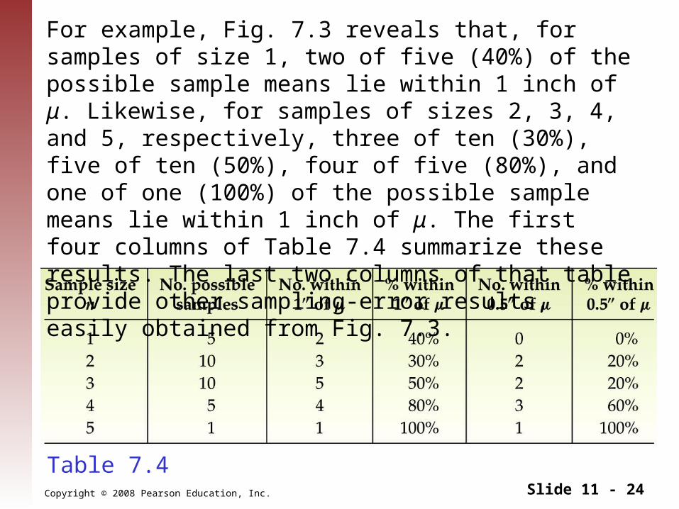
Table 7.4
For example, Fig. 7.3 reveals that, for samples of size 1, two of five (40%) of the possible sample means lie within 1 inch of μ. Likewise, for samples of sizes 2, 3, 4, and 5, respectively, three of ten (30%), five of ten (50%), four of five (80%), and one of one (100%) of the possible sample means lie within 1 inch of μ. The first four columns of Table 7.4 summarize these results. The last two columns of that table provide other sampling-error results, easily obtained from Fig. 7.3.

Copyright © 2008 Pearson Education, Inc. Slide 12 - 24
Key Fact 7.1

Copyright © 2008 Pearson Education, Inc. Slide 13 - 24
Formula 7.1

Copyright © 2008 Pearson Education, Inc. Slide 14 - 24
Formula 7.2

Copyright © 2008 Pearson Education, Inc. Slide 15 - 24
Solution Example 7.7First, we apply Formula 7.1 and Formula 7.2 to conclude that μ = μ = 100 and σ = 8; that is, the variable has mean 100 and standard deviation 8.
Example 7.7
Intelligence quotients (IQs) measured on the Stanford Revision of the Binet-Simon Intelligence Scale are normally distributed with mean 100 and standard deviation 16. For a sample size of 4, use simulation to make plausible the fact that is normally distributed.x
x xx

Copyright © 2008 Pearson Education, Inc. Slide 16 - 24Output 7.1
Solution Example 7.7
We simulated 1000 samples of four IQs each, determined the sample mean of each of the 1000 samples, and obtained a histogram (Output 7.1) of the 1000 samplemeans. We also superimposed on the histogram the normal distribution with mean 100 and standard deviation 8. The histogram is shaped roughly like a normal curve.
Copyright © 2008 Pearson Education, Inc. Slide 17 - 24
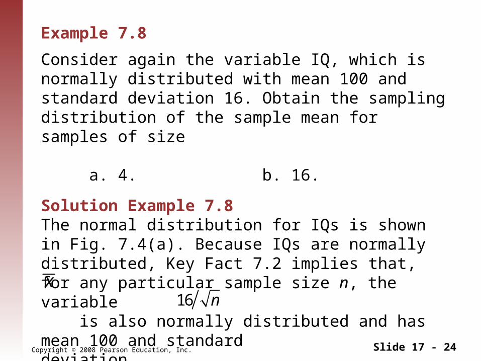
Solution Example 7.8The normal distribution for IQs is shown in Fig. 7.4(a). Because IQs are normally distributed, Key Fact 7.2 implies that, for any particular sample size n, the variable is also normally distributed and has mean 100 and standard deviation .
Example 7.8
Consider again the variable IQ, which is normally distributed with mean 100 and standard deviation 16. Obtain the sampling distribution of the sample mean for samples of size
a. 4. b. 16.
x16 n

Copyright © 2008 Pearson Education, Inc. Slide 18 - 24
Figure 7.4
Solution Example 7.8a. For samples of size 4, we have σ = 8, and therefore the sampling distribution of the sample mean is a normal distribution with mean100 and standard deviation 8. Figure7.4(b) shows this normal distribution.

Copyright © 2008 Pearson Education, Inc. Slide 19 - 24
Figure 7.4
Solution Example 7.8b. For samples of size16, we have σ = 4, and therefore the sampling distribution of the sample mean is a normal distribution with mean100 and standard deviation 4. Figure7.4(c) shows this normal distribution.

Copyright © 2008 Pearson Education, Inc. Slide 20 - 24
Table 7.7
Example 7.9
According to the U.S. Census Bureau publication Current Population Reports, a frequency distribution for the number of people per household in the United States is as displayed in Table 7.7. Frequencies are in millions of households.
Here, the variable is household size, and the population is all U.S. households. From Table 7.7, we find that the mean household size is μ = 2.685 persons and the standard deviation is σ = 1.47 persons.

Copyright © 2008 Pearson Education, Inc. Slide 21 - 24
Figure 7.5
Example 7.9
Figure 7.5 is a relative-frequency histogram for household size, obtained from Table 7.7. Note that household size is far from being normally distributed; it is right skewed. Nonetheless, according to the central limit theorem, the sampling distribution of the sample mean can beapproximated by a normal distribution when the sample size is relatively large. Use simulation to make that fact plausible for a sample size of 30.
Copyright © 2008 Pearson Education, Inc. Slide 22 - 24
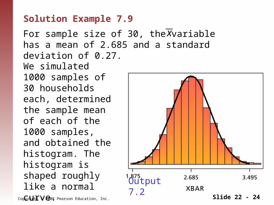
Solution Example 7.9
For sample size of 30, the variable has a mean of 2.685 and a standard deviation of 0.27.
Output 7.2
We simulated 1000 samples of 30 households each, determined the sample mean of each of the 1000 samples, and obtained the histogram. The histogram is shaped roughly like a normal curve.
x

Copyright © 2008 Pearson Education, Inc. Slide 23 - 24
Key Fact 7.4

Copyright © 2008 Pearson Education, Inc. Slide 24 - 24
Figure 7.6