Slide 1 South-Western Publishing Applications of Cost Theory Chapter 9 Estimation of Cost Functions...

South-Western Publishing

Applications of Cost TheoryChapter 9

• Estimation of Cost Functions using regressions» Short run -- various methods including polynomial functions» Long run -- various methods including

• Engineering cost techniques

• Survivor techniques

• Break-even analysis and operating leverage• Risk assessment• Appendix 9A: The Learning Curve

Estimating Costs in the SR

• Typically use TIME SERIES data for a plant or firm.

• Typically use a functional form that “fits” the presumed shape.

• For TC, often CUBIC

• For AC, often QUADRATIC

quadratic is U-shaped or arch shaped.

cubic is S-shapedor backward S-shaped

Estimating Short Run Cost Functions

• Example: TIME SERIES data of total cost

• Quadratic Total Cost (to the power of two)

TC = C0 + C1 Q + C2 Q2

TC Q Q 2

900 20 400

800 15 225

834 19 361

REGR c1 1 c2 c3

TimeSeriesData

Predictor Coeff Std Err T-value

Constant 1000 300 3.3Q -50 20 -2.5Q-squared 10 2.5 4.0

R-square = .91Adj R-square = .90N = 35

Regression Output:

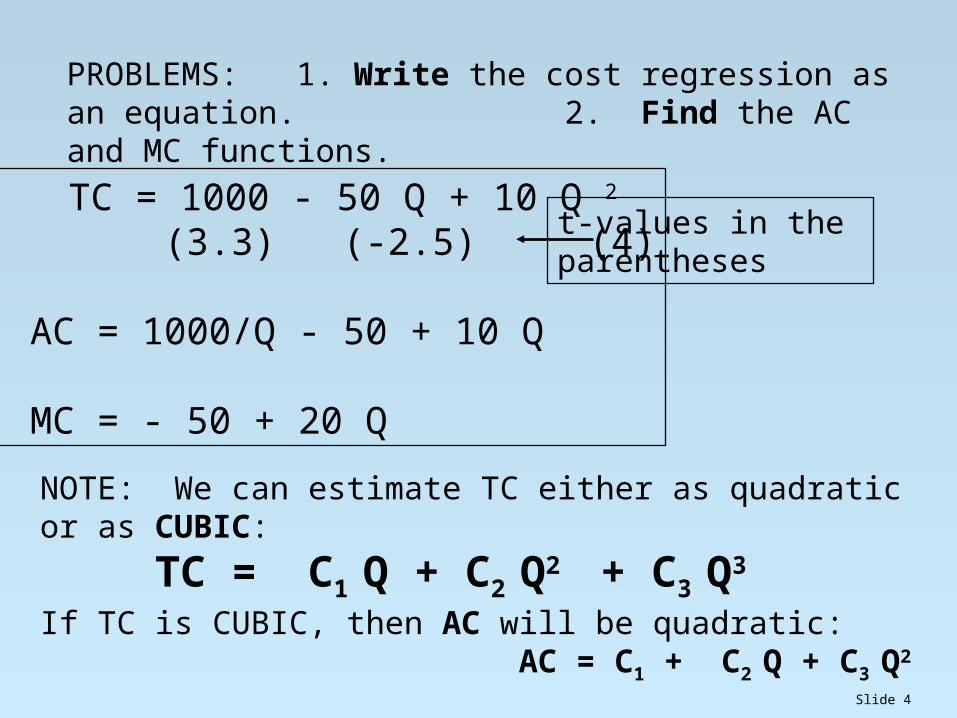
PROBLEMS: 1. Write the cost regression as an equation. 2. Find the AC and MC functions.

1. TC = 1000 - 50 Q + 10 Q 2

(3.3) (-2.5) (4)

2. AC = 1000/Q - 50 + 10 Q

MC = - 50 + 20 Q

t-values in the parentheses

NOTE: We can estimate TC either as quadratic or as CUBIC:

TC = C1 Q + C2 Q2 + C3 Q3

If TC is CUBIC, then AC will be quadratic: AC = C1 + C2 Q + C3 Q2

What Went Wrong With Boeing?• Airbus and Boeing both produce large capacity passenger

jets• Boeing built each 747 to order, one at a time, rather than

using a common platform» Airbus began to take away Boeing’s market share through its

lower costs.

• As Boeing shifted to mass production techniques, cost fell, but the price was still below its marginal cost for wide-body planes

Estimating LR Cost Relationships

• Use a CROSS SECTION of firms» SR costs usually

uses a time series

• Assume that firms are near their lowest average cost for each output

Q

AC

LRAC

Log Linear LR Cost Curves• One functional form is Log Linear

• Log TC = a + b• Log Q + c•Log W + d•Log R• Coefficients are elasticities.• “b” is the output elasticity of TC

» IF b = 1, then CRS long run cost function

» IF b < 1, then IRS long run cost function

» IF b > 1, then DRS long run cost function

Example: Electrical Utilities

Sample of 20 UtilitiesQ = megawatt hoursR = cost of capital on rate base, W = wage rate

Electrical Utility ExampleElectrical Utility Example

• Regression Results:Log TC = -.4 +.83 Log Q + 1.05 Log(W/R)

(1.04) (.03) (.21)

R-square = .9745Std-errors are inthe parentheses

QUESTIONS:

1. Are utilities constant returns to scale?

2. Are coefficients statistically significant?

3. Test the hypothesis:

Ho: b = 1.

A n s w e r s

1.The coefficient on Log Q is less than one. A 1% increase in output lead only to a .83% increase in TC -- It’s Increasing Returns to Scale!

2.The t-values are coeff / std-errors: t = .83/.03 = 27.7 is Sign. & t = 1.05/.21 = 5.0 which is Significant.

3.The t-value is (.83 - 1)/.03 = - 0.17/.03 = - 5.6 which is significantly different than CRS.

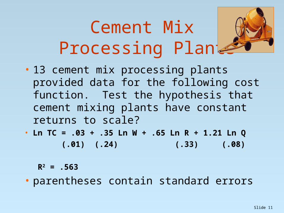
Cement Mix Processing Plants

• 13 cement mix processing plants provided data for the following cost function. Test the hypothesis that cement mixing plants have constant returns to scale?

• Ln TC = .03 + .35 Ln W + .65 Ln R + 1.21 Ln Q

(.01) (.24) (.33) (.08)

R2 = .563

• parentheses contain standard errors

Discussion• Cement plants are Constant Returns if the

coefficient on Ln Q were 1

• 1.21 is more than 1, which appears to be Decreasing Returns to Scale.

• TEST: t = (1.21 -1 ) /.08 = 2.65

• Small Sample, d.f. = 13 - 3 -1 = 9

• critical t = 2.262

• We reject constant returns to scale.

Engineering Cost Approach

• Engineering Cost Techniques offer an alternative to fitting lines through historical data points using regression analysis.

• It uses knowledge about the efficiency of machinery.

• Some processes have pronounced economies of scale, whereas other processes (including the costs of raw materials) do not have economies of scale.

• Size and volume are mathematically related, leading to engineering relationships. Large warehouses tend to be cheaper than small ones per cubic foot of space.

Survivor Technique• The Survivor Technique examines what size of firms

are tending to succeed over time, and what sizes are declining.

• This is a sort of Darwinian survival test for firm size.• Presently many banks are merging, leading one to

conclude that small size offers disadvantages at this time.

• Dry cleaners are not particularly growing in average size, however.

Break-even Analysis & D.O.LBreak-even Analysis & D.O.L• Can have multiple B/E points• If linear total cost and total

revenue:» TR = P•Q» TC = F + v•Q

• where v is Average Variable Cost

• F is Fixed Cost

• Q is Output

• cost-volume-profit analysis

TotalCost

TotalRevenue

B/E B/EQ

The Break-even Quantity: Q B/E

• At break-even: TR = TC» So, P•Q = F + v•Q

• Q B/E = F / ( P - v) = F/CM» where contribution margin is:

CM = ( P - v)

TR

TC

B/E Q

PROBLEM: As a garagecontractor, find Q B/E

if: P = $9,000 per garage v = $7,000 per garage& F = $40,000 per year

• Amount of sales revenues that breaks even

• P•Q B/E = P•[F/(P-v)]

= F / [ 1 - v/P ]

Break-even Sales Volume

Variable Cost Ratio

Ex: At Q = 20, B/E Sales Volume is $9,000•20 = $180,000 Sales Volume

Answer: Q = 40,000/(2,000)= 40/2 = 20 garages at the break-even point.

Target Profit Output Quantity needed to attain a target

profit If is the target profit,

Q target = [ F + ] / (P-v)

Suppose want to attain $50,000 profit, then,

Q target = ($40,000 + $50,000)/$2,000

= $90,000/$2,000 = 45 garages

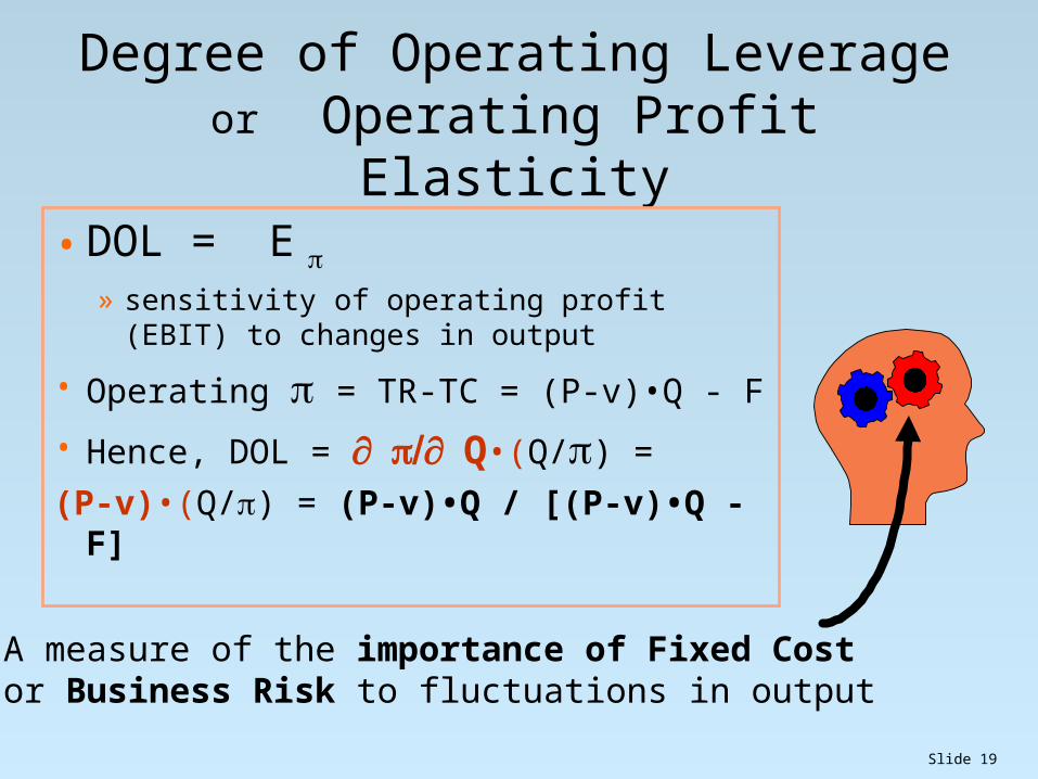
Degree of Operating Leverageor Operating Profit Elasticity

• DOL = E» sensitivity of operating profit (EBIT) to

changes in output

• Operating = TR-TC = (P-v)•Q - F

• Hence, DOL = Q•(Q/) =

(P-v)•(Q/) = (P-v)•Q / [(P-v)•Q - F]

A measure of the importance of Fixed Costor Business Risk to fluctuations in output

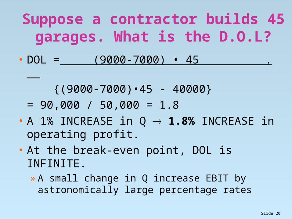
Suppose a contractor builds 45 garages. What is the D.O.L?

• DOL = (9000-7000) • 45 .

{(9000-7000)•45 - 40000}

= 90,000 / 50,000 = 1.8

• A 1% INCREASE in Q 1.8% INCREASE in operating profit.

• At the break-even point, DOL is INFINITE. » A small change in Q increase EBIT by

astronomically large percentage rates

DOL as Operating Profit Elasticity

DOL = [ (P - v)Q ] / { [ (P - v)Q ] - F }• We can use empirical estimation methods to find

operating leverage

• Elasticities can be estimated with double log functional forms

• Use a time series of data on operating profit and output» Ln EBIT = a + b• Ln Q, where b is the DOL» then a 1% increase in output increases EBIT by b%

» b tends to be greater than or equal to 1

Regression Output• Dependent Variable: Ln EBIT uses 20 quarterly observations N =

20

The log-linear regression equation isLn EBIT = - .75 + 1.23 Ln Q

Predictor Coeff Stdev t-ratio pConstant -.7521 0.04805 -15.650 0.001Ln Q 1.2341 0.1345 9.175 0.001s = 0.0876 R-square= 98.2% R-sq(adj) = 98.0%

The DOL for this firm, 1.23. So, a 1% increase in output leads to a 1.23% increase in operating profit

Operating Profit and the Business Cycle

Output

recession

TIME

EBIT =operating profit

Trough

peak

1. EBIT is more volatilethat output over cycle

2. EBIT tends to collapse late in recessions

Learning Curve: Appendix 9A• “Learning by doing” has wide application in production

processes. • Workers and management become more efficient with

experience.

• the cost of production declines as the accumulated past production, Q = qt, increases, where qt is

the amount produced in the tth period. • Airline manufacturing, ship building, and appliance

manufacturing have demonstrated the learning curve effect.

• Functionally, the learning curve relationship can be written C = a·Qb, where C is the input cost of the Qth unit:

• Taking the (natural) logarithm of both sides, we get: log C = log a + b·log Q

• The coefficient b tells us the extent of the learning curve effect.» If the b=0, then costs are at a constant level.» If b > 0, then costs rise in output, which is exactly

opposite of the learning curve effect.» If b < 0, then costs decline in output, as predicted by

the learning curve effect.

Slide 1 South-Western Publishing Applications of Cost Theory Chapter 9 Estimation of Cost Functions...

Documents

Transcript of Slide 1 South-Western Publishing Applications of Cost Theory Chapter 9 Estimation of Cost Functions...