AUTOREGRESSIVE AUGMENTATION OF MIDAS REGRESSIONS · MIDAS regressions see Andreou et al., 2011)....

working papers

1 | 2014

JANUARY 2014

The analyses, opinions and fi ndings of these papers represent

the views of the authors, they are not necessarily those of the

Banco de Portugal or the Eurosystem

AUTOREGRESSIVE AUGMENTATION OF MIDAS REGRESSIONS

Cláudia Duarte

Please address correspondence to

Banco de Portugal, Economics and Research Department

Av. Almirante Reis 71, 1150-012 Lisboa, Portugal

Tel.: 351 21 313 0000, email: [email protected]

BANCO DE PORTUGAL

Av. Almirante Reis, 71

1150-012 Lisboa

www.bportugal.pt

Edition

Economics and Research Department

Lisbon, 2014

ISBN 978-989-678-269-6 (online)

ISSN 2182-0422 (online)

Legal Deposit no. 3664/83

Autoregressive augmentation of MIDAS regressions∗

Claudia Duarte†

Banco de PortugalISEG-UTL

January 2014

Abstract

Focusing on the MI(xed) DA(ta) S(ampling) regressions for handling different samplingfrequencies and asynchronous releases of information, alternative techniques for the autoregressiveaugmentation of these regressions are presented and discussed. For forecasting quarterly euroarea GDP growth using a small set of selected indicators, the results obtained suggest that nospecific kind of MIDAS regressions clearly dominates in terms of forecast accuracy. Nevertheless,alternatives to common-factor MIDAS regressions with autoregressive terms perform well and insome cases are the best performing regressions.

Keywords: MIDAS regressions, High-frequency data, Autoregressive terms, Forecasting

JEL Codes: C53, E37

∗The author is grateful to Joao Nicolau and Paulo Rodrigues for thoughtful discussions and helpful comments. Thispaper benefits from comments of participants at the 24th (EC)2 Conference “The Econometrics Analysis of MixedFrequency Data” held at the University of Cyprus. Comments by Carlos Robalo Marques and Christian Schumacheron previous versions of the paper are also gratefully acknowledged. A special thanks to Fatima Teodoro for softwareassistance. The usual disclaimers apply.†Corresponding author. Postal address: Banco de Portugal - Research Department, Rua Francisco Ribeiro 2, 1150-

012 Lisboa - Portugal; Tel: +351 213130934; Fax: +351 213107804; E-mail: [email protected]

1 Introduction

Inspired in the distributed lag models, the MI(xed) DA(ta) S(ampling) framework,

proposed by Ghysels et al. (2004), is a very flexible tool for dealing with different time

frequencies, asynchronous releases of information, different aggregation polynomials

and different forecast horizons (for a brief overview of the main topics related with

MIDAS regressions see Andreou et al., 2011).

MIDAS regressions were originally associated with empirical applications to financial

series, focusing on volatility predictions; see Ghysels et al. (2004, 2006, 2007).

However, MIDAS regressions have also been used in typical macroeconomic forecasting

applications (see, among others, Clements and Galvao, 2008 and Bai et al., 2013 for

US GDP growth, Armesto et al., 2009 for the predictive content of the Beige Book,

Kuzin et al., 2011 for euro area GDP, Marcellino and Schumacher, 2010 for German

GDP, Monteforte and Moretti, 2013 for euro area inflation, and Asimakopoulos et al.,

2013 for fiscal variables of a set of European countries).

The inclusion of autoregressive dynamics is an important feature of forecasting models,

especially for macroeconomic applications. Ghysels et al. (2007) and Andreou et al.

(2011) pointed out that the autoregressive distributed lag MIDAS regression entails an

undesirable property - discontinuities in the impulse response function of the regressor

(x(m)t ) on the variable of interest (Yt). To tackle this issue, Clements and Galvao

(2008) suggested interpreting the dynamics on Yt as a common factor (Hendry and

Mizon, 1978). This assumption rests on the hypothesis that Yt and x(m)t share the

same autoregressive dynamics, though, as Hendry and Mizon (1978) pointed out, a

common factor may not always be found.

The main aim of this article is to discuss alternative techniques for introducing

autoregressive terms in MIDAS regressions. The initial contributions on this issue are

reassessed and an alternative approach is proposed. It is claimed that standard MIDAS

regressions (no common factor restriction) are able to deal with autoregressive terms,

without jeopardising the pattern of the impulse response functions from x(m)t on Yt.

The sequence of coefficients associated with lags of x(m)t , retrieved from the distributed

lag representation of MIDAS regressions, is not the relevant impulse response function.

Inspired by the periodic model framework (see Hansen and Sargent (2013) and Ghysels

(2012), among others), one can say that there are several impulse response functions,

one for each high-frequency period within a low-frequency observation. The observed

low-frequency impulse response functions do not exhibit discontinuities, regardless of

the lags of x(m)t or Yt included in the regression.

2

Furthermore, the empirical performance of alternative MIDAS regressions with

autoregressive terms is evaluated through a forecasting exercise. For forecasting

quarterly euro area GDP growth, the performance of an extended set of MIDAS

regressions, in terms of root mean squared forecast error (RMSFE), is assessed through

a horse race. Simple AR and traditional low-frequency models are used as benchmarks.

MIDAS regressions without autoregressive terms are also included for comparison

reasons. As the evidence in favour of using large information sets is not clear-cut

(see, for example, Banerjee and Marcellino, 2006), this article focuses on a small set of

selected indicators.

The forecasts are obtained through a recursive out-of-sample exercise, which takes

into account the ragged-edges of the high-frequency data and the publication delay of

GDP. To assess whether the gains in terms of forecast accuracy from taking on board

high-frequency data are short-lived, past high-frequency data is combined to obtain

nowcasts (current period forecasts) and direct forecasts for different horizons, up to

4 quarters ahead. The results obtained suggest that alternatives to common-factor

MIDAS regressions with autoregressive terms perform well, being in some cases the

best performing regressions.

The remainder of this paper is organised as follows. Section 2 describes the main

topics related with MIDAS modelling and discusses in detail the different techniques

for the autoregressive augmentation of MIDAS regressions. The design of the now-

and forecasting exercise is presented in section 3, while section 4 focuses on the results.

Finally, section 5 concludes.

2 MIDAS modelling

In this section, after presenting some theoretical motivation and notation (section

2.1), the MIDAS approach is discussed in section 2.2. Then, in section 2.3 the initial

contributions on introducing autoregressive terms in MIDAS regressions are reviewed

and an alternative perspective on this issue is proposed.

2.1 Background

Consider the traditional low frequency regression,

Yt+h = α + βQt + εt+h (1)

where h denotes the forecast horizon (when h = 0 the model delivers nowcasts) and

both Yt+h and Qt are sampled at a low frequency, e.g., quarterly. All the parameters of

3

the model depend on the forecast horizon and forecasts are computed directly, i.e., no

additional forecasts of the explanatory variables are needed in order to obtain forecasts

for the variable of interest. Equation 1 can be extended to include lags of the Y and

Q variables, as well as additional regressors and respective lags.

Now, assume that Yt+h and Qt are temporal aggregates of higher frequency disaggreg-

ated series, e.g., monthly series (yt+h and xt, respectively). For each low-frequency

(quarterly) observation of Yt+h and Qt there are m (3) observations of the high-

frequency (monthly) yt+h and xt series. The low-frequency variables are characterised

by an aggregation scheme Γ(L1/m). There are different schemes, e.g., stock variables

or flow variables with equal weights. In the following analysis an unrestricted linear

combination of γi weights will be considered.

In time series analysis, observed time series are often temporal aggregates of unobserved

disaggregated series. As before, assume for instance that Qt is observed monthly (xt),

while Yt+h is only observed quarterly - meaning that yt+h is not observed (flow variable)

or has missing observations (stock variable). Although regression analysis would ideally

try to approximate the original data generating process (DGP) by using high-frequency

samples, as in the following equation

g(L1/m)yt+h = a+N∑i=1

bi(L1/m)xi,t + et+h (2)

where g(L1/m) and bi(L1/m) are finite order lag polynomials, this is not always possible.

The mixed-frequency approaches suggest mixing a low-frequency dependent variable

on the left-hand side with high-frequency regressors on the right-hand side. Assuming

that high-frequency yt+h would be well represented by equation 2, there is a φ(L1/m)

polynomial such that h(L) = g(L1/m)φ(L1/m). Multiplying both sides of equation 2 by

φ(L1/m) and the aggregation scheme Γ(L1/m) one obtains

φ(L1/m)g(L1/m)Γ(L1/m)yt+h = a+N∑i=1

bi(L1/m)φ(L1/m)Γ(L1/m)xi,t

+ φ(L1/m)Γ(L1/m)et+h

h(L)Yt+h = a+N∑i=1

bi(L1/m)zi,t + ξt+h (3)

where a = φ(L1/m)Γ(L1/m)a, zi,t = φ(L1/m)Γ(L1/m)xi,t, ξt+h = φ(L1/m)Γ(L1/m)et+h

and t = m, 2m, 3m, .... Equation 3 is the exact mixed-frequency model associated with

the high-frequency model in equation 2, relating the low-frequency Yt+h dependent

variable with the high-frequency xi,t regressors.

4

As discussed in Wei and Stram, 1990, Marcellino, 1998 and Marcellino, 1999, among

others, in general it is not possible to uniquely identify φ(L1/m) in this single-equation

framework and, so, neither the g(L1/m) and bi(L1/m) polynomials. This means that, in

general, one can only approximate the mixed-frequency model, as follows

h(L)Yt+h = a+N∑i=1

bi(L1/m)x

(3)i,t + ut+h (4)

where x(3)i,t is the skip-sampled version of the high-frequency xi,t and the orders of

the polynomials h(L) and bi(L1/m) are data-driven (e.g., selected from information

criteria). Furthermore, since one cannot recover the high-frequency g(L1/m) and

bi(L1/m) polynomials, it is also not possible to identify the high-frequency impulse

response function of xi,t on yt. Hence, the approximate mixed-frequency model implies

an observable quarterly impulse response function of x(3)i,t on Yt. Underlying this

observable impulse response function are the latent monthly impulse response functions

of xi,t on yt.

2.2 From the approximate mixed-frequency regression to MIDAS regres-sions

Equation 4 is a MIDAS regression. More precisely, equation 4 as been referred to in the

literature as an unrestricted MIDAS regression; see e.g. Marcellino and Schumacher

(2010), Foroni and Marcellino (2012) and Foroni et al. (2011). This regression is

one of the particular cases covered by the general MIDAS framework. Introduced by

Ghysels et al. (2004) and initially presented in Ghysels et al. (2006) or Ghysels et al.

(2007), the MIDAS approach provides simple, reduced-form models to approximate

more elaborate, though unknown, high-frequency models. Original MIDAS regressions

assume that the coefficients of bi(L1/m) in equation 4 are captured by a known weight

function B(j; θ),

Yt+h = β0 + β1B(L1/m; θ)x(3)t + ut+h (5)

where B(L1/m; θ) =∑J

j=0B(j; θ)Lj/m is a polynomial of length J in the L1/m operator,

B(j; θ) represents the weighting scheme used for the aggregation, which is assumed to

be normalised to sum to 1, β1 is the slope coefficient, β0 is a constant, Lj/mx(m)t = x

(m)t−j/m

and ut+h is a standard iid error term.

Although the order of the polynomial B(L1/m; θ), i.e. J , is potentially infinite, some

restrictions must be imposed for the sake of tractability. The restrictions result from

the need of a balance between the gains in terms of additional information (more lags)

and the costs of parameter proliferation. Information criteria, such as AIC and BIC,

5

can be used to guide this choice. In the original MIDAS regressions, the coefficients of

B(L1/m; θ) are captured by a known weighting function B(j; θ), which depends on a

few parameters summarised in vector θ.

For example, Ghysels et al. (2007) considered two alternatives for the weighting

function, both assuming that the weights are determined by a few hyperparameters

θ: the exponential Almon lag

B(j; θ1, θ2) =e(θ1j+θ2j2)∑Ji=1 e

(θ1i+θ2i2)(6)

and the beta polynomial

B(j; θ1, θ2) =f( j

J, θ1, θ2)∑J

i=1 f( iJ, θ1, θ2)

(7)

where f(q, θ1, θ2) = (qθ1−1(1−q)θ2−1Γ(θ1 +θ2))/(Γ(θ1)Γ(θ2)) and Γ(θ) =∫∞

0e−kkθ−1dk.

Given that exponential Almon and beta polynomials have nonlinear functional

specifications, in both cases MIDAS regressions have to be estimated using nonlinear

methods, namely nonlinear least squares.

Chen and Ghysels (2010) discussed a multiplicative MIDAS framework, which is closer

to traditional aggregation. Instead of aggregating all lags in the high frequency variable

to a single aggregate, multiplicative MIDAS regressions include m-aggregates of high-

frequency data and their lags,

Yt+h = β0 +

p∑i=1

βi+1xmultt−i + ut+h (8)

where xmultt =∑m−1

j=0 B(j; θ)Lj/mx(m)t .

Another aggregation scheme is the one underlying the above-mentioned unrestricted

MIDAS regressions, resulting in MIDAS regressions that can be estimated by OLS.

Yt+h = β0 +Bu(L1/m)x

(m)t + ut+h

= β0 +J∑j=0

βj+1Lj/mx

(m)t + ut+h

= β0 + β1x(m)t + β2x

(m)t−1/m + . . .+ βJ+1x

(m)t−J/m + ut+h. (9)

When the difference between the low and the high frequency is large, estimating a

regression such as equation 9 can involve a large number of parameters. In this case,

large differences in sampling frequencies between the variables considered are readily

penalised in terms of parsimony. For instance, if Yt+h is sampled quarterly and xt

6

refers to daily data, then estimating a mixed-frequency regression can easily involve

estimating more than 60 parameters.

Summing up, MIDAS regressions allow more flexible weighting structure than tra-

ditional low-frequency models and can also be more parsimonious. Moreover, the

MIDAS framework can easily accommodate the timely releases of high-frequency data.

In (5), where Yt+h and x(m)t are contemporaneously related, it is assumed that all high-

frequency observations over the current low-frequency period are known. Considering

quarterly and monthly data, this means that the three months in the quarter are

already available. If instead of a full-quarter, say, only the first month is available,

then the MIDAS regression can be rewritten as

Yt+h = β0 + β1B(L1/3; θ)x(3)t−2/3 + ut+h. (10)

2.3 Autoregressive augmentation of MIDAS regressions

In section 2.3.1 initial contributions to the literature regarding the introduction

of autoregressive terms in MIDAS regressions are reviewed, while an alternative

perspective on this subject is presented in section 2.3.2. For the sake of simplicity

and unless otherwise stated, a first order autoregression and h = 0 are assumed.

Notwithstanding, the notation can be easily extended.

2.3.1 Initial contributions

Ghysels et al. (2007) discussed the implications of introducing autoregressive terms in

MIDAS regressions and suggested two possible ways of doing this, noting that both

solutions had caveats. In the first case, a polynomial in L1/m is considered,

Yt = β0 + β1B(L1/m; θ)x(m)t + γYt−(1/m) + ut (11)

which implicitly assumes that Yt−(1/m) is available. This solution may not be very

appealing because if high-frequency lags of Yt were available then probably it would be

possible to set up a high-frequency regression. Moreover, Ghysels et al. (2007) remarked

that estimating (11) is more challenging because including the term Yt−(1/m) forces one

to deal with endogenous regressors and with instrumental variable estimation.

In the second case, a polynomial in L is considered, i.e.

Yt = β0 + β1B(L1/m; θ)x(m)t + γYt−1 + ut

Yt = β∗0 + β1B(L1/m; θ)

(1 − γL)x

(m)t + u∗t (12)

7

where B(L1/m; θ) =∑J

j=0B(j; θ)Lj/m, β∗0 = β0/(1 − γ) and u∗t = ut/(1 − γL).

Considering the distributed lag representation, instead of a polynomial in L1/m one

obtains a mixture B(L1/m;θ)(1−γL)

. Equation 13 shows more clearly the shape of the

polynomial, for example assuming J = m− 1 = 2 for the sake of simplicity, we can see

that

Yt = β∗0 + β1(B0x(3)t +B1x

(3)t−1/3 +B2x

(3)t−2/3 + γB0x

(3)t−1 + γB1x

(3)t−4/3 + γB2x

(3)t−5/3

+γ2B0x(3)t−2 + γ2B1x

(3)t−7/3 + γ2B2x

(3)t−8/3 + ...) + u∗t (13)

Ghysels et al. (2007) and Andreou et al. (2011) pointed out that the autoregressive

distributed lag MIDAS regression in equation 12 entails an undesirable property - theB(L1/m;θ)

(1−γL)polynomial displays geometrically declining spikes at distance m, mimicking

a seasonal pattern. This autoregressive augmentation of MIDAS regressions should be

used if a seasonal pattern in x(m)t is detected (Ghysels et al., 2007).

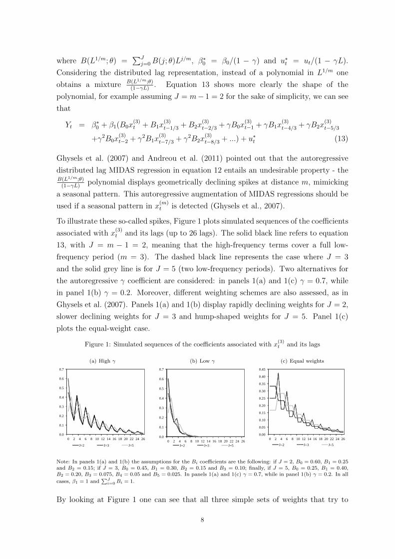
To illustrate these so-called spikes, Figure 1 plots simulated sequences of the coefficients

associated with x(3)t and its lags (up to 26 lags). The solid black line refers to equation

13, with J = m − 1 = 2, meaning that the high-frequency terms cover a full low-

frequency period (m = 3). The dashed black line represents the case where J = 3

and the solid grey line is for J = 5 (two low-frequency periods). Two alternatives for

the autoregressive γ coefficient are considered: in panels 1(a) and 1(c) γ = 0.7, while

in panel 1(b) γ = 0.2. Moreover, different weighting schemes are also assessed, as in

Ghysels et al. (2007). Panels 1(a) and 1(b) display rapidly declining weights for J = 2,

slower declining weights for J = 3 and hump-shaped weights for J = 5. Panel 1(c)

plots the equal-weight case.

Figure 1: Simulated sequences of the coefficients associated with x(3)t and its lags

(a) High γ

0.0

0.1

0.2

0.3

0.4

0.5

0.6

0.7

0 2 4 6 8 10 12 14 16 18 20 22 24 26

J=2 J=3 J=5

(b) Low γ

0.0

0.1

0.2

0.3

0.4

0.5

0.6

0.7

0 2 4 6 8 10 12 14 16 18 20 22 24 26J=2 J=3 J=5

(c) Equal weights

0.00

0.05

0.10

0.15

0.20

0.25

0.30

0.35

0.40

0.45

0 2 4 6 8 10 12 14 16 18 20 22 24 26

J=2 J=3 J=5

Note: In panels 1(a) and 1(b) the assumptions for the Bi coefficients are the following: if J = 2, B0 = 0.60, B1 = 0.25and B2 = 0.15; if J = 3, B0 = 0.45, B1 = 0.30, B2 = 0.15 and B3 = 0.10; finally, if J = 5, B0 = 0.25, B1 = 0.40,B2 = 0.20, B3 = 0.075, B4 = 0.05 and B5 = 0.025. In panels 1(a) and 1(c) γ = 0.7, while in panel 1(b) γ = 0.2. In all

cases, β1 = 1 and∑J

i=0Bi = 1.

By looking at Figure 1 one can see that all three simple sets of weights that try to

8

mimic the polynomial weighting schemes display a spiky pattern and, as expected, this

pattern is softened with smaller γ. Note that with unrestricted MIDAS the pattern

could be even more irregular, as the weights/coefficients are estimated unrestrictedly,

not obeying to a known polynomial function. In the traditional case of equal-weight

schemes, the sequence of coefficients have a stepwise pattern, except when the number

of high-frequency terms do not fully cover low-frequency periods (e.g. when J = 3),

which also exhibits spikes.

Clements and Galvao (2008) suggested an alternative way of introducing autoregressive

dynamics in MIDAS regressions. The authors proposed interpreting the dynamics on Yt

as a common factor (Hendry and Mizon, 1978). This assumption rests on the hypothesis

that Yt and x(m)t share the same autoregressive dynamics, though, as Hendry and Mizon

(1978) pointed out, a common factor may not always be found. Hence, considering

Yt = β0 + β1B(L1/m; θ)x(m)t + ut

ut = γut−1 + εt (14)

and replacing ut in (14) it follows that

(1 − γL)Yt = β0(1 − γ) + β1(1 − γL)B(L1/m; θ)x(m)t + εt (15)

When writing (15) in the distributed lag representation, the polynomial in L cancels

out, leaving the polynomial in L1/m. The coefficients β0, β1, θ and γ are estimated

together, using nonlinear least squares in a two-step approach. First, the initial value

for γ can be estimated as

ut = γut−1 + εt (16)

where ut are the residuals from a static MIDAS regression (without autoregressive

terms) and εt is an error term iid (0, σ2). The estimates for γ are used to filter the

original Yt and x(m)t variables. Second, the filtered variables are used to estimate β0,

β1 and θ in a static MIDAS regression. Although the initial work by Clements and

Galvao (2008) and subsequent empirical applications (see, for example, Marcellino

and Schumacher, 2010, Kuzin et al., 2011, Foroni and Marcellino, 2012, Jansen et al.,

2012, Monteforte and Moretti, 2013 and Kuzin et al., 2013) only consider a single

autoregressive term, in this paper this technique was extended to allow for more

autoregressive terms. This can be done by including the additional lags of the residuals

u in (16), as follows

ut =

p∑i=1

γiut−i + εt. (17)

9

2.3.2 Alternative perspective

The literature presented so far suggests that adding autoregressive terms to MIDAS

regressions in such a way that generates a B(L1/m;θ)(1−γL)

polynomial implies declining spikes

at distance m in the infinite sequence of coefficients associated with x(m)t and its lags.

However, should this sequence be perceived as the relevant impulse response function

from the high-frequency variable on the low-frequency variable?

To answer this question let us start by assuming that xt and yt are both observed at

the high frequency, say monthly. Furthermore, assume that the DGP is known and

resumes to an autoregressive term of order one, the contemporaneous variable xt and

two lags (xt−1/3 and xt−2/3). To ease the exposition, the time index remains unaltered,

so that the monthly time index is expressed by t = 0, 1/3, 2/3, 1, 4/3, . . . , T .

yt = α + b0xt + b1xt−1/3 + b2xt−2/3 + λyt−1/3 + ut (18)

The distributed lag version of this equation can be written as

yt = α∗ + b0xt + (b1 + λb0)xt−1/3 +∞∑i=0

λi(b2 + λb1 + λ2b0)xt−(2+i)/3 + u∗t (19)

where α∗ = α/(1 − λL1/3) and u∗t = ut/(1 − λL1/3). Consider a shock equal to 1 in x

in January 2012. The response on the y variable in January 2012 is equal to b0. The

responses in February and March are b1 + λb0 and b2 + λb1 + λ2b0, respectively. So,

considering a generic aggregation scheme Γ(L1/m), the response in the first quarter is

equal to b0γ0 + (b1 + λb0)γ1 + (b2 + λb1 + λ2b0)γ2. Similarly, the monthly responses in

April, May and June are λ(b2 +λb1 +λ2b0), λ2(b2 +λb1 +λ2b0) and λ3(b2 +λb1 +λ2b0),

respectively, resulting in a response of (λ3β0 + λ2β1 + λβ2)(γ0 + γ1λ + γ2λ2) in the

second quarter.

The exact mixed-frequency regression can be obtained by pre-multiplying (18) by the

finite order polynomials φ(L1/3) and Γ(L1/3). Assume that the autoregressive order in

the low/quarterly frequency is also one. In this case, φ(L1/3) = (1 + λL1/3 + λ2L2/3),

i.e., φ(L1/3)(1 − λL1/3) = 1 − λ3L. So, applying both polynomials one obtains the

following mixed-frequency regression

(1−λ3L)Yt = α+δ0xt+δ1xt−1/3+δ2xt−2/3+δ3xt−1+δ4xt−4/3+δ5xt−5/3+δ6xt−2+ut (20)

where δ0 = b0γ2, δ1 = b0(γ1 +λγ2) + b1γ2, δ2 = b0(γ0 +λγ1 +λ2γ2) + b1(γ1 +λγ2) + b2γ2,

δ3 = b0(λγ0 +λ2γ1) + b1(γ0 +λγ1 +λ2γ2) + b2(γ1 +λγ2), δ4 = b0λ2γ0 + b1(λγ0 +λ2γ1) +

b2(γ0 + λγ1 + λ2γ2), δ5 = b1λ2γ0 + b2(λγ0 + λ2γ1) and δ6 = b2λ

2γ0.

10

Writing this equation in a distributed lag form one obtains

Yt = α+ δ0xt + δ1xt−1/3 + δ2xt−2/3

+ (δ3 + λ3δ0)xt−1+ (δ4 + λ3δ1)xt−4/3 + (δ5 + λ3δ2)xt−5/3

+ (δ6 + λ3δ3 + λ6δ0)xt−2+λ3(δ4 + λ3δ1)xt−7/3 +λ3(δ5 + λ3δ2)xt−8/3

+λ3(δ6 + λ3δ3 + λ6δ0)xt−3+λ6(δ4 + λ3δ1)xt−10/3+λ6(δ5 + λ3δ2)xt−11/3

+λ6(δ6 + λ3δ3 + λ6δ0)xt−4+λ9(δ4 + λ3δ1)xt−13/3+λ9(δ5 + λ3δ2)xt−14/3+...+ ut

(21)

where α = α/(1−λ3L) and ut = ut/(1−λ3L). Again, consider a shock equal to 1 in x

in January 2012. The response on the Y variable in the first quarter of 2012 is equal

to δ2, which corresponds to b0(γ0 + λγ1 + λ2γ2) + b1(γ1 + λγ2) + b2γ2. Rearranging the

terms, this response equals the quarterly aggregate response underlying the monthly

regression. A similar result is obtained for the following period - the response on the

Y variable in the second quarter of 2012 is δ5 + λ3δ2, which also equals the quarterly

aggregate of the monthly responses in April, May and June. The same reasoning

is also valid if shocks in other months or combined shocks in more than one month

were considered. These results can be extended to different specifications and to other

forecast horizons.

As regards impulse response functions from x(m)t on Yt, sequentially assessing the

coefficients in (21) does not seem to be very informative. The sequence δ0, δ1, δ2,

(δ3 + λ3δ0), ... - with or without spikes - cannot be considered the relevant impulse

response function because some of the coefficients (in this case, sets of three non-

overlapping parameters) refer to the same time period in the low frequency, i.e., to the

same quarter. Furthermore, recall that each coefficient in this sequence already covers

the relevant latent monthly impulse responses on y within each quarterly observation

of Y , for each monthly shock in x.

Inspired by the periodic model framework (see Hansen and Sargent (2013) and Ghysels

(2012), among others), one can say that there are several impulse response functions,

one for each m high-frequency period within a low-frequency observation. For example,

in (21), the observed quarterly impulse response function from a shock in the first month

of the quarter on the quarterly Yt variable is δ2, δ5 + λ3δ2, λ3(δ5 + λ3δ2), λ6(δ5 + λ3δ2),

and so on and so forth. Similarly, the observed quarterly impulse response function

from a shock in the second month of the quarter on the quarterly Yt variable is δ1,

δ4 + λ3δ1, λ3(δ4 + λ3δ1), λ6(δ4 + λ3δ1), ..., and so on. Any of the observed quarterly

impulse response functions do not exhibit spikes, regardless of the lags of x(m)t or Yt

included in the regression.

11

When the number of high-frequency lags in the mixed-frequency regressions is multiple

of m minus 1 (or lower than m− 1) there is homogeneity in the shape of the impulse

response functions on Yt, regardless of the type of shock in x(m)t . This means that

all impulse response functions share the same geometric decay pattern, i.e., the decay

starts at the same time. In cases where the number of high-frequency lags is greater

than m−1 but not its multiple, such as equation 20, the shape of the impulse response

functions varies with the high-frequency timing of the shock in x(m)t - for shocks in the

first and second months of the quarter the geometric decay starts after two quarters,

while for shocks in the third month of the quarter that decay only starts after three

quarters.

Note that, as mentioned before, in a single-equation environment, one cannot recover

the monthly impulse response functions of xt on yt departing from the mixed-frequency

regression. Moreover, this framework only analyses the transmission of changes in one

direction, from the high-frequency variables to the low-frequency variable, not taking

into account the possible relation between the high-frequency variables nor the impact

of changes in the low-frequency variable into the high-frequency variables.

In light of this discussion, alternatives to the common factor way of introducing autore-

gressive terms in MIDAS regressions can be considered. In particular, generalizing

conventional ADL regressions, autoregressive terms are added to MIDAS regressions,

without restrictions - not imposing the common factor, no restrictions on both the

lag structure and the order of the autoregressive polynomial - see Andreou et al.

(2013) and Guerin and Marcellino (2013). Moreover, no restrictions are imposed on

the aggregation scheme - exponential Almon weight function, unrestricted (Foroni and

Marcellino, 2012) and multiplicative (Francis et al., 2011).

Furthermore, in the same vein of multiplicative MIDAS regressions, which closely

map the traditional low frequency model (i.e., reverse engineering the low frequency

regressions, replacing the time aggregates by the underlying combinations of high-

frequency lags, results in a mixed-frequency regression with a number of high-frequency

lags that is always a multiple of m minus 1) the performance of original and unrestricted

MIDAS regressions with autoregressive terms and with high-frequency lags multiple of

m minus 1 is also analysed.

The latter regressions require full quarter information to be available, including for the

current quarter. In order to implement these regressions when the m current-period

high-frequency observations have not been released, the series of the regressors with

unbalanced m periods were stacked with forecasts obtained from simple autoregressive

regressions. Given that MIDAS regressions deliver direct forecasts, the autoregressive

12

extrapolation of regressors is also based on direct forecasting. Note that this bridge

approach to MIDAS regressions can be easily implemented for, say, monthly regressors.

However, this procedure is less feasible when the regressors have time frequencies

higher than monthly. This approach somehow mimics the state-space approach, with

the simple autoregressive regressions acting as the state equation, and the MIDAS

regression as the observation equation. Nevertheless, as in the traditional bridge model

framework, this two-step approach is hindered by orthogonality issues, which can lead

to biases in coefficient estimates.

Note that this latter version of MIDAS regressions ensures that the geometric decay

pattern starts at the same time in all m impulse response functions. Moreover, when

new information becomes available within the current quarter, there is no need to

change the forecasting regression in order to update the forecasts. This procedure only

involves substituting the stacked regressor forecasts by the newly observed figures.

3 Design of the nowcasting and forecasting exercise

The aim of this exercise is to nowcast and forecast quarterly developments in euro

area GDP growth, in real terms, using three different indicators: a hard-data series;

a soft-data series; and a financial series. Thus, the dataset used contains a quarterly

series on the real GDP from 1996Q1 to 2012Q4, the monthly industrial production and

the monthly economic sentiment indicator from January 1996 to December 2012, and

the Dow Jones Euro Stoxx index on a daily basis from 1 January 1996 to 31 December

2012. All series are seasonally adjusted except the stock market information. Apart

from the economic sentiment indicator, the original series were transformed, using the

rate of change (based on the first difference), in order to have stationary variables.

The data considered are final data, meaning that they refer to the latest release

available when the database was built. While in the case of the economic sentiment

indicator and the stock market index final data equal real-time data, as these series

are not revised, revisions of GDP and industrial production are not taken into account

in this analysis. However, evidence from previous work on data revisions suggests that

revisions are typically small for euro area GDP (Marcellino and Musso, 2011).

The database is split in two, for the in-sample estimation and the out-of-sample

forecasting exercise. From 1996Q1 to 2006Q4 the sample was used for in-sample model

specification and estimation. Different types of MIDAS regressions were estimated -

original, multiplicative, with and without autoregressive terms - based on different

information sets.1 Different lags were considered (up to 4 quarters), also for the1The codes used to estimate and forecast using MIDAS regressions were written in Matlab. Some functions were

13

autoregressive terms. All regressions were recursively estimated and selected using

information criteria, namely the BIC.

In the following analysis the original MIDAS regressions, as in equation 5, will be simply

denoted as “MIDAS”. Moreover, the multiplicative (equation 8) and unrestricted

(equation 9) regressions are denoted as “M-MIDAS” and “U-MIDAS”, respectively.

The MIDAS specification with common factor autoregressive dynamics (equation 15)

will be labelled “CF-MIDAS”, while without that restriction the prefix “AR-” is

added. The case of MIDAS regressions with autoregressive terms and with high-

frequency lags multiple of m minus 1 will have the prefix “Balanced”. Apart from U-

MIDAS regressions, all other MIDAS regressions were estimated using the exponential

Almon polynomial defined as in equation 6.2 Different initial parameter specifications

(including the equal weight hypothesis, i.e. θ1 = θ2 = 0) were tested and the results

do not differ significantly (for a discussion on the shapes of different weighting sets, see

Ghysels et al., 2007). The hyperparameters θ of the exponential Almon function are

restricted to θ1 < 5 and θ2 < 0.

The sample from 2007Q1 to 2012Q4 was used for the out-of-sample nowcasting and

forecasting exercise. Although an out-of-sample forecast exercise with P = 24 quarters

has limitations, using euro area data still bears an inevitable trade-off between sample

sizes for in-sample and out-of-sample exercises and this forecasting exercise is no

exception. For obtaining the forecasts, a recursive exercise was performed, so that

throughout the out-of-sample period the estimation sample is recursively expanded by

adding one observation at a time. As a new observation is added to the estimation

sample, the regressions are re-estimated and, thus, the coefficients are allowed to change

over time. Adding to nowcasts (h = 0) direct forecast for up to h = 4 quarters ahead

are also presented. For each forecast horizon a different model is estimated.

Although the database used is not a real-time database, the different publication lags

of the indicators are taken into account when within-quarter information is used. So,

in a single-variable framework, it is possible to have up to 3 different forecasts for a

given quarter, for each quarterly forecast horizon, depending on the within-quarter

information used - one month (I), two months (II), or full quarter (III).

To evaluate the forecasting performance of the different MIDAS regressions is used the

root mean squared forecast error (RMSFE). Relative RMSFE are computed to compare

the performance of the MIDAS approach with alternative, purely quarterly, benchmark

models. Two benchmark models are considered. The first is an autoregressive (AR)

taken from the Econometrics Toolbox written by James P. LeSage (http://www.spatial-econometrics.com). The MIDAStoolbox used was greatly inspired in a code kindly provided by Arthur Sinko.

2The beta polynomial was also tested and the results were qualitatively similar. All results are available from theauthor upon request.

14

model, which is estimated recursively, using a general-to-specific approach, and the lag

length (from 0 to 4 lags) is chosen according to information criteria, namely the BIC.

The AR benchmark boils down to the sample average when, according to the BIC

criterion, including positive lags leads to a worse performance than choosing the lag

length equal to 0.

The second is a traditional quarterly single-equation multivariate model, with all the

variables in the low frequency. This model includes autoregressive terms (from 0 to

4 lags) and is also estimated recursively, using a general-to-specific approach and the

BIC. As different information sets are considered (different variables) the quarterly

multivariate models are adjusted accordingly. Moreover, when full quarter information

is not available, forecasts from the quarterly multivariate models are obtained through

a bridge model framework, in this case with a direct forecasting approach, similarly

to MIDAS approach. So, estimates for the missing monthly observations, obtained

from univariate models, are plugged in the monthly data, which are transformed into

quarterly series and, then, used for forecasting in the traditional quarterly model. To

ensure consistency within all forecasts used, the missing monthly observations are also

direct forecasts from autoregressive models.

In order to assess the statistical significance of the differences in the forecasting

performance between the alternatives considered, the test of equal forecast accuracy on

the population-level of direct multi-step forecasts from nested linear models proposed

by Clark and McCracken (2005) is used. The null hypothesis is that the benchmark

model forecasts (restricted model, denoted as model 1) are as accurate as those of

the MIDAS regressions (unrestricted model, denoted as model 2) and the one-sided

alternative hypothesis is that the unrestricted model forecasts are more accurate.

Following the authors’ notation, the test statistic used is

MSE − F = PMSE1 −MSE2

MSE2

(22)

where P is the number of forecasts and MSEi denotes the mean squared forecast error

of model i, with i = 1, 2. Because this test has a non-standard limiting distribution,

a bootstrap procedure was implemented to obtain the critical values. As suggested by

Clark and McCracken (2005) and similarly to Kilian (1999), the bootstrap algorithm

used starts with the estimation of a large set of simulated samples of the dependent

variable (1000 samples), which are computed by drawing with replacement from the

sample residuals under the null hypothesis (restricted model). Moreover, a bootstrap-

after-bootstrap procedure, as proposed by Kilian (1998), is implemented to obtain

small-sample bias-adjusted bootstrapped time series. Based on this simulated data,

both restricted and unrestricted direct multi-step forecasts are calculated recursively

15

and the test statistic is computed for each set of forecasts. The critical values are

computed as quantiles of the bootstrapped series of test statistics.

4 Empirical results

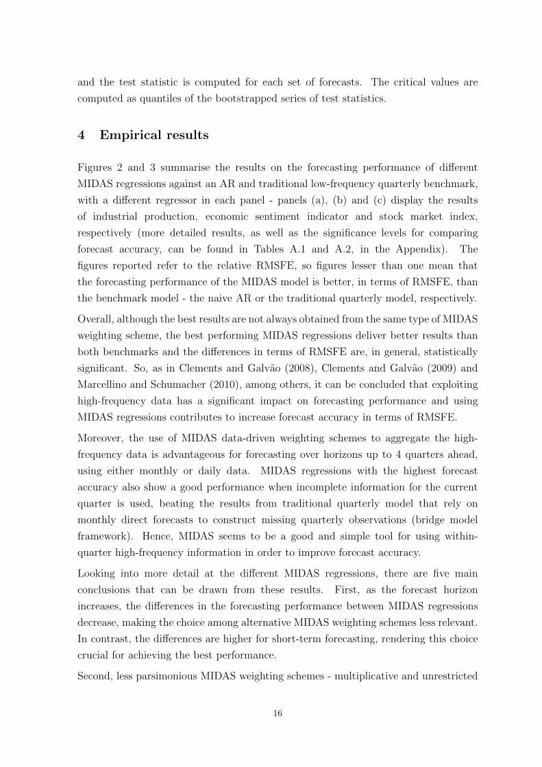
Figures 2 and 3 summarise the results on the forecasting performance of different

MIDAS regressions against an AR and traditional low-frequency quarterly benchmark,

with a different regressor in each panel - panels (a), (b) and (c) display the results

of industrial production, economic sentiment indicator and stock market index,

respectively (more detailed results, as well as the significance levels for comparing

forecast accuracy, can be found in Tables A.1 and A.2, in the Appendix). The

figures reported refer to the relative RMSFE, so figures lesser than one mean that

the forecasting performance of the MIDAS model is better, in terms of RMSFE, than

the benchmark model - the naive AR or the traditional quarterly model, respectively.

Overall, although the best results are not always obtained from the same type of MIDAS

weighting scheme, the best performing MIDAS regressions deliver better results than

both benchmarks and the differences in terms of RMSFE are, in general, statistically

significant. So, as in Clements and Galvao (2008), Clements and Galvao (2009) and

Marcellino and Schumacher (2010), among others, it can be concluded that exploiting

high-frequency data has a significant impact on forecasting performance and using

MIDAS regressions contributes to increase forecast accuracy in terms of RMSFE.

Moreover, the use of MIDAS data-driven weighting schemes to aggregate the high-

frequency data is advantageous for forecasting over horizons up to 4 quarters ahead,

using either monthly or daily data. MIDAS regressions with the highest forecast

accuracy also show a good performance when incomplete information for the current

quarter is used, beating the results from traditional quarterly model that rely on

monthly direct forecasts to construct missing quarterly observations (bridge model

framework). Hence, MIDAS seems to be a good and simple tool for using within-

quarter high-frequency information in order to improve forecast accuracy.

Looking into more detail at the different MIDAS regressions, there are five main

conclusions that can be drawn from these results. First, as the forecast horizon

increases, the differences in the forecasting performance between MIDAS regressions

decrease, making the choice among alternative MIDAS weighting schemes less relevant.

In contrast, the differences are higher for short-term forecasting, rendering this choice

crucial for achieving the best performance.

Second, less parsimonious MIDAS weighting schemes - multiplicative and unrestricted

16

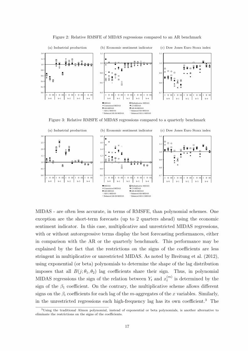
Figure 2: Relative RMSFE of MIDAS regressions compared to an AR benchmark

(a) Industrial production

0.0

0.2

0.4

0.6

0.8

1.0

1.2

1.4

I II III I II III I II III I II III I II III

h=0 h=1 h=2 h=3 h=4

(b) Economic sentiment indicator

0.4

0.6

0.8

1.0

1.2


h=0 h=1 h=2 h=3 h=4

MIDAS Multiplicative MIDASUnrestricted MIDAS CF-MIDASAR-MIDAS AR-M-MIDASAR-U-MIDAS Balanced AR-MIDASBalanced AR-M-MIDAS Balanced AR-U-MIDAS

(c) Dow Jones Euro Stoxx index

0.7

0.8

0.9

1.0

1.1


h=0 h=1 h=2 h=3 h=4

Figure 3: Relative RMSFE of MIDAS regressions compared to a quarterly benchmark

(a) Industrial production

0.0

0.5

1.0

1.5

2.0

2.5

3.0


h=0 h=1 h=2 h=3 h=4

(b) Economic sentiment indicator

0.6

0.8

1.0

1.2

1.4

1.6

1.8


h=0 h=1 h=2 h=3 h=4

MIDAS Multiplicative MIDASUnrestricted MIDAS CF-MIDASAR-MIDAS AR-M-MIDASAR-U-MIDAS Balanced AR-MIDASBalanced AR-M-MIDAS Balanced AR-U-MIDAS

(c) Dow Jones Euro Stoxx index

0.7

0.8

0.9

1.0

1.1

1.2


h=0 h=1 h=2 h=3 h=4

MIDAS - are often less accurate, in terms of RMSFE, than polynomial schemes. One

exception are the short-term forecasts (up to 2 quarters ahead) using the economic

sentiment indicator. In this case, multiplicative and unrestricted MIDAS regressions,

with or without autoregressive terms display the best forecasting performances, either

in comparison with the AR or the quarterly benchmark. This performance may be

explained by the fact that the restrictions on the signs of the coefficients are less

stringent in multiplicative or unrestricted MIDAS. As noted by Breitung et al. (2012),

using exponential (or beta) polynomials to determine the shape of the lag distribution

imposes that all B(j; θ1, θ2) lag coefficients share their sign. Thus, in polynomial

MIDAS regressions the sign of the relation between Yt and x(m)t is determined by the

sign of the β1 coefficient. On the contrary, the multiplicative scheme allows different

signs on the βi coefficients for each lag of the m-aggregates of the x variables. Similarly,

in the unrestricted regressions each high-frequency lag has its own coefficient.3 The

3Using the traditional Almon polynomial, instead of exponential or beta polynomials, is another alternative toeliminate the restrictions on the signs of the coefficients.

17

estimation results from the traditional quarterly models confirm that changing signs

in the lag coefficients is an important feature in the regressions using the economic

sentiment indicator, for forecast horizons up to 2 quarter ahead.

Third, the best performing MIDAS regressions tend to include autoregressive terms,

which is an expected result given that this empirical application uses macroeconomic

data (Clements and Galvao, 2008, Marcellino and Schumacher, 2010, Monteforte

and Moretti, 2013, among others). Fourth, focusing on MIDAS regressions with

autoregressive terms, the results suggest that it is possible to improve forecasting per-

formance of MIDAS regressions by using weighting schemes alternative to CF-MIDAS.

In particular, up to 1 quarter ahead, balanced AR-U-MIDAS consistently outperforms

CF-MIDAS in the regressions using the economic sentiment indicator. Note that this

performance is observed even when full-quarter information is not available, which

suggests that combining balanced MIDAS regressions with autoregressive extrapolation

of the regressor can deliver good results in terms of forecast accuracy in the short term.

Also for short-term forecasting, AR-MIDAS regressions with the Dow Jones Euro Stoxx

index have the best forecasting performance, being a good alternative for dealing with

autoregressive augmentation. In the case of industrial production, the evidence is more

mixed and no clear pattern is detected. Nevertheless, in 7 out of 15 cases the alternative

models to CF-MIDAS show the best forecasting performance.

Finally, the existence of some degree of variability in the ranking of forecasting per-

formance among alternative MIDAS regressions with autoregressive terms, especially

in the short term, suggests that choosing is essentially an empirical question. It may be

the case that in some empirical exercises imposing a common factor dynamics between

Yt and x(m)t can be less benign than using alternative ways of including autoregressive

terms in MIDAS regressions. In other cases it may be the opposite.

5 Conclusion

Having started on the financial field, MIDAS regressions have been gaining an

increasing attention in macroeconomic forecasting. This technique is a simple, flexible

and potentially parsimonious way of taking into account timely releases of high-

frequency data, in particular for forecasting a low-frequency series. Nevertheless,

the autoregressive augmentation of MIDAS regressions has raised some concerns. In

this paper, alternative ways of dealing with autoregressive augmentation of MIDAS

regression are discussed. It is shown that standard MIDAS regressions (no common

factor restriction) are able to deal with autoregressive terms.

18

Moreover, the forecasting performance, in terms of RMSFE, of several kinds of MIDAS

regressions is assessed through a recursive forecasting exercise. The benchmarks used

are a simple autoregressive model and traditional quarterly models. In the latter

case, a bridge model framework was put in place whenever full-quarter information

was not available. Corroborating previous evidence, the results obtained suggest that

using MIDAS regressions contributes to increase forecast accuracy. The statistically

significant benefits from this data-driven, and potentially more parsimonious, weighting

scheme to aggregate the high-frequency data are obtained for forecast horizons up to

4 quarter ahead, regardless of having incomplete information for the current quarter

and of the exact time frequency of the regressors.

The results also stress the importance of choosing the best MIDAS model for each

specific situation, namely when the aim is short-term forecasting. The auxiliary choices

of the forecaster when using MIDAS regressions are, thus, crucial for the success in

nowcasting and forecasting exercises. Although there is no one-fits-all recipe, the

results suggests that the multiplicative and unrestricted MIDAS seem to be a good

alternative to the original (polynomial) MIDAS regressions when restrictions on signs

of the coefficients play an important role. Furthermore, focusing on MIDAS regressions

with autoregressive terms, imposing a common factor dynamics between the dependent

variable and the regressors (CF-MIDAS) can be, in some cases, too strict. The other

ways of introducing autoregressive terms in MIDAS regressions analysed in this paper

- AR-MIDAS, AR-M-MIDAS, AR-U-MIDAS and the respective balanced versions -

proved to be good alternatives and in some cases are the best performing MIDAS

regression.

19

References

Andreou, E., Ghysels, E. and Kourtellos, A. (2011), Forecasting with mixed-frequency

data, in M. Clements and D. Hendry, eds, ‘The Oxford Handbook of Economic

Forecasting’, Oxford University Press, chapter 8, pp. 225–267.

Andreou, E., Ghysels, E. and Kourtellos, A. (2013), ‘Should macroeconomic forecasters

use daily financial data and how?’, Journal of Business and Economic Statistics (31).

Armesto, M. T., Hernandez-Murillo, R., Owyang, M. T. and Piger, J. (2009),

‘Measuring the information content of the Beige Book: A mixed data sampling

approach’, Journal of Money, Credit and Banking 41(1), 35–55.

Asimakopoulos, S., Paredes, J. and Warmedinger, T. (2013), Forecasting fiscal time

series using mixed frequency data, Working Paper Series 1550, European Central

Bank.

Bai, J., Ghysels, E. and Wright, J. H. (2013), ‘State space models and MIDAS

regressions’, Econometric Reviews 32(7), 779–813.

Banerjee, A. and Marcellino, M. (2006), ‘Are there any reliable leading indicators for

US inflation and GDP growth?’, International Journal of Forecasting 22(1), 137–151.

Breitung, J., Elengikal, S. and Roling, C. (2012), Forecasting inflation rates using daily

data: A nonparametric MIDAS approach, mimeo.

Chen, X. and Ghysels, E. (2010), ‘News — good or bad — and its impact on volatility

predictions over multiple horizons’, The Review of Financial Studies 23(1), 46–81.

Clark, T. and McCracken, M. (2005), ‘Evaluating direct multistep forecasts’,

Econometric Reviews 24(4), 369–404.

Clements, M. and Galvao, A. (2008), ‘Macroeconomic forecasting with mixed-frequency

data: Forecasting output growth in the United States’, Journal of Business and

Economic Statistics 26(4), 546–554.

Clements, M. and Galvao, A. (2009), ‘Forecasting US output growth using leading

indicators: An appraisal using MIDAS models’, Journal of Applied Econometrics

24, 1187–1206.

Foroni, C. and Marcellino, M. (2012), A comparison of mixed frequency approaches

for modelling euro area macroeconomic variables, Economics Working Papers

ECO2012/07, European University Institute.

20

Foroni, C., Marcellino, M. and Schumacher, C. (2011), U-MIDAS: MIDAS regressions

with unrestricted lag polynomials, Discussion Paper Series 1: Economic Studies

2011,35, Deutsche Bundesbank, Research Centre.

Francis, N., Ghysels, E. and Owyang, M. T. (2011), The low-frequency impact of daily

monetary policy shocks, Working Papers 2011-009, Federal Reserve Bank of St. Louis.

Ghysels, E. (2012), Macroeconomics and the reality of mixed frequency data, mimeo.

Ghysels, E., Santa-Clara, P. and Valkanov, R. (2004), The MIDAS touch: Mixed data

sampling regression models, CIRANO Working Papers 2004s-20, CIRANO.

Ghysels, E., Santa-Clara, P. and Valkanov, R. (2006), ‘Predicting volatility: getting the

most out of return data sampled at different frequencies’, Journal of Econometrics

131, 59–95.

Ghysels, E., Sinko, A. and Valkanov, R. (2007), ‘MIDAS regressions: Further results

and new directions’, Econometric Reviews 26(1), 53–90.

Guerin, P. and Marcellino, M. (2013), ‘Markov-switching MIDAS models’, Journal of

Business & Economic Statistics 31(1), 45–56.

Hansen, L. and Sargent, T. J. (2013), Recursive Models of Dynamic Linear Economies,

forthcoming edn, Princeton University Press.

Hendry, D. F. and Mizon, G. E. (1978), ‘Serial correlation as a convenient simplification,

not a nuisance: A comment on a study of the demand for money by the Bank of

England’, The Economic Journal 88(351), 549–563.

Jansen, J., Jin, X. and de Winter, J. (2012), Forecasting and nowcasting real GDP:

comparing statistical models and subjective forecasts, DNB Working Paper 365, De

Nederlandsche Bank.

Kilian, L. (1998), ‘Small-sample confidence intervals for impulse response functions’,

The Review of Economics and Statistics 80(2), 218–230.

Kilian, L. (1999), ‘Exchange rates and monetary fundamentals: What do we learn from

long-horizon regressions?’, Journal of Applied Econometrics 14(5), pp. 491–510.

Kuzin, V., Marcellino, M. and Schumacher, C. (2011), ‘MIDAS versus mixed-frequency

VAR: Nowcasting GDP in the euro area’, International Journal of Forecasting

27, 529–542.

Kuzin, V., Marcellino, M. and Schumacher, C. (2013), ‘Pooling versus model selection

for nowcasting GDP with many predictors: Empirical evidence for six industrialized

countries’, Journal of Applied Econometrics 28(3), 392–411.

21

Marcellino, M. (1998), ‘Temporal disaggregation, missing observations, outliers and

forecasting: a unifying non-model based procedure’, Advances in Econometrics

13, 181–202.

Marcellino, M. (1999), ‘Consequences of temporal aggregation in empirical analysis’,

Journal of Business and Economic Statistics 17(1), 129–136.

Marcellino, M. and Musso, A. (2011), ‘The reliability of real-time estimates of the euro

area output gap’, Economic Modelling 28(4), 1842–1856.

Marcellino, M. and Schumacher, C. (2010), ‘Factor MIDAS for nowcasting and

forecasting with ragged-edge data: A model comparison for German GDP’, Oxford

Bulletin of Economics and Statistics 72(4), 518–550.

Monteforte, L. and Moretti, G. (2013), ‘Real-time forecasts of inflation: The role of

financial variables’, Journal of Forecasting 32(1), 51–61.

Wei, W. W. S. and Stram, D. O. (1990), ‘Disaggregation of time series models’, Journal

of the Royal Statistical Society. Series B (Methodological) 52(3), pp. 453–467.

22

Appendix

23

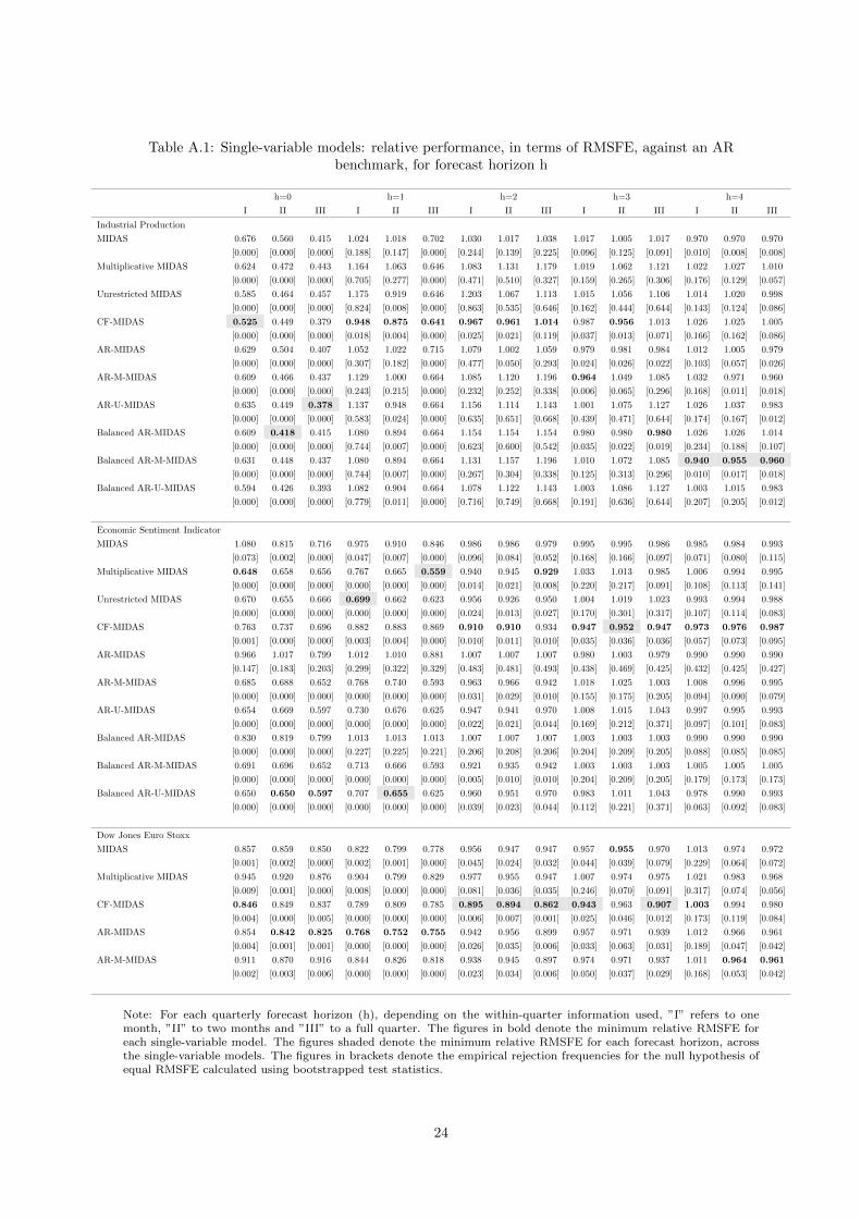
Table A.1: Single-variable models: relative performance, in terms of RMSFE, against an ARbenchmark, for forecast horizon h

h=0 h=1 h=2 h=3 h=4


Industrial Production

MIDAS 0.676 0.560 0.415 1.024 1.018 0.702 1.030 1.017 1.038 1.017 1.005 1.017 0.970 0.970 0.970

[0.000] [0.000] [0.000] [0.188] [0.147] [0.000] [0.244] [0.139] [0.225] [0.096] [0.125] [0.091] [0.010] [0.008] [0.008]

Multiplicative MIDAS 0.624 0.472 0.443 1.164 1.063 0.646 1.083 1.131 1.179 1.019 1.062 1.121 1.022 1.027 1.010

[0.000] [0.000] [0.000] [0.705] [0.277] [0.000] [0.471] [0.510] [0.327] [0.159] [0.265] [0.306] [0.176] [0.129] [0.057]

Unrestricted MIDAS 0.585 0.464 0.457 1.175 0.919 0.646 1.203 1.067 1.113 1.015 1.056 1.106 1.014 1.020 0.998

[0.000] [0.000] [0.000] [0.824] [0.008] [0.000] [0.863] [0.535] [0.646] [0.162] [0.444] [0.644] [0.143] [0.124] [0.086]

CF-MIDAS 0.525 0.449 0.379 0.948 0.875 0.641 0.967 0.961 1.014 0.987 0.956 1.013 1.026 1.025 1.005

[0.000] [0.000] [0.000] [0.018] [0.004] [0.000] [0.025] [0.021] [0.119] [0.037] [0.013] [0.071] [0.166] [0.162] [0.086]

AR-MIDAS 0.629 0.504 0.407 1.052 1.022 0.715 1.079 1.002 1.059 0.979 0.981 0.984 1.012 1.005 0.979

[0.000] [0.000] [0.000] [0.307] [0.182] [0.000] [0.477] [0.050] [0.293] [0.024] [0.026] [0.022] [0.103] [0.057] [0.026]

AR-M-MIDAS 0.609 0.466 0.437 1.129 1.000 0.664 1.085 1.120 1.196 0.964 1.049 1.085 1.032 0.971 0.960

[0.000] [0.000] [0.000] [0.243] [0.215] [0.000] [0.232] [0.252] [0.338] [0.006] [0.065] [0.296] [0.168] [0.011] [0.018]

AR-U-MIDAS 0.635 0.449 0.378 1.137 0.948 0.664 1.156 1.114 1.143 1.001 1.075 1.127 1.026 1.037 0.983

[0.000] [0.000] [0.000] [0.583] [0.024] [0.000] [0.635] [0.651] [0.668] [0.439] [0.471] [0.644] [0.174] [0.167] [0.012]

Balanced AR-MIDAS 0.609 0.418 0.415 1.080 0.894 0.664 1.154 1.154 1.154 0.980 0.980 0.980 1.026 1.026 1.014

[0.000] [0.000] [0.000] [0.744] [0.007] [0.000] [0.623] [0.600] [0.542] [0.035] [0.022] [0.019] [0.234] [0.188] [0.107]

Balanced AR-M-MIDAS 0.631 0.448 0.437 1.080 0.894 0.664 1.131 1.157 1.196 1.010 1.072 1.085 0.940 0.955 0.960

[0.000] [0.000] [0.000] [0.744] [0.007] [0.000] [0.267] [0.304] [0.338] [0.125] [0.313] [0.296] [0.010] [0.017] [0.018]

Balanced AR-U-MIDAS 0.594 0.426 0.393 1.082 0.904 0.664 1.078 1.122 1.143 1.003 1.086 1.127 1.003 1.015 0.983

[0.000] [0.000] [0.000] [0.779] [0.011] [0.000] [0.716] [0.749] [0.668] [0.191] [0.636] [0.644] [0.207] [0.205] [0.012]

Economic Sentiment Indicator

MIDAS 1.080 0.815 0.716 0.975 0.910 0.846 0.986 0.986 0.979 0.995 0.995 0.986 0.985 0.984 0.993

[0.073] [0.002] [0.000] [0.047] [0.007] [0.000] [0.096] [0.084] [0.052] [0.168] [0.166] [0.097] [0.071] [0.080] [0.115]


[0.000] [0.000] [0.000] [0.000] [0.000] [0.000] [0.014] [0.021] [0.008] [0.220] [0.217] [0.091] [0.108] [0.113] [0.141]


[0.000] [0.000] [0.000] [0.000] [0.000] [0.000] [0.024] [0.013] [0.027] [0.170] [0.301] [0.317] [0.107] [0.114] [0.083]

CF-MIDAS 0.763 0.737 0.696 0.882 0.883 0.869 0.910 0.910 0.934 0.947 0.952 0.947 0.973 0.976 0.987

[0.001] [0.000] [0.000] [0.003] [0.004] [0.000] [0.010] [0.011] [0.010] [0.035] [0.036] [0.036] [0.057] [0.073] [0.095]

AR-MIDAS 0.966 1.017 0.799 1.012 1.010 0.881 1.007 1.007 1.007 0.980 1.003 0.979 0.990 0.990 0.990

[0.147] [0.183] [0.203] [0.299] [0.322] [0.329] [0.483] [0.481] [0.493] [0.438] [0.469] [0.425] [0.432] [0.425] [0.427]

AR-M-MIDAS 0.685 0.688 0.652 0.768 0.740 0.593 0.963 0.966 0.942 1.018 1.025 1.003 1.008 0.996 0.995

[0.000] [0.000] [0.000] [0.000] [0.000] [0.000] [0.031] [0.029] [0.010] [0.155] [0.175] [0.205] [0.094] [0.090] [0.079]

AR-U-MIDAS 0.654 0.669 0.597 0.730 0.676 0.625 0.947 0.941 0.970 1.008 1.015 1.043 0.997 0.995 0.993

[0.000] [0.000] [0.000] [0.000] [0.000] [0.000] [0.022] [0.021] [0.044] [0.169] [0.212] [0.371] [0.097] [0.101] [0.083]


[0.000] [0.000] [0.000] [0.227] [0.225] [0.221] [0.206] [0.208] [0.206] [0.204] [0.209] [0.205] [0.088] [0.085] [0.085]


[0.000] [0.000] [0.000] [0.000] [0.000] [0.000] [0.005] [0.010] [0.010] [0.204] [0.209] [0.205] [0.179] [0.173] [0.173]


[0.000] [0.000] [0.000] [0.000] [0.000] [0.000] [0.039] [0.023] [0.044] [0.112] [0.221] [0.371] [0.063] [0.092] [0.083]

Dow Jones Euro Stoxx

MIDAS 0.857 0.859 0.850 0.822 0.799 0.778 0.956 0.947 0.947 0.957 0.955 0.970 1.013 0.974 0.972

[0.001] [0.002] [0.000] [0.002] [0.001] [0.000] [0.045] [0.024] [0.032] [0.044] [0.039] [0.079] [0.229] [0.064] [0.072]


[0.009] [0.001] [0.000] [0.008] [0.000] [0.000] [0.081] [0.036] [0.035] [0.246] [0.070] [0.091] [0.317] [0.074] [0.056]

CF-MIDAS 0.846 0.849 0.837 0.789 0.809 0.785 0.895 0.894 0.862 0.943 0.963 0.907 1.003 0.994 0.980

[0.004] [0.000] [0.005] [0.000] [0.000] [0.000] [0.006] [0.007] [0.001] [0.025] [0.046] [0.012] [0.173] [0.119] [0.084]

AR-MIDAS 0.854 0.842 0.825 0.768 0.752 0.755 0.942 0.956 0.899 0.957 0.971 0.939 1.012 0.966 0.961

[0.004] [0.001] [0.001] [0.000] [0.000] [0.000] [0.026] [0.035] [0.006] [0.033] [0.063] [0.031] [0.189] [0.047] [0.042]

AR-M-MIDAS 0.911 0.870 0.916 0.844 0.826 0.818 0.938 0.945 0.897 0.974 0.971 0.937 1.011 0.964 0.961

[0.002] [0.003] [0.006] [0.000] [0.000] [0.000] [0.023] [0.034] [0.006] [0.050] [0.037] [0.029] [0.168] [0.053] [0.042]

Note: For each quarterly forecast horizon (h), depending on the within-quarter information used, ”I” refers to onemonth, ”II” to two months and ”III” to a full quarter. The figures in bold denote the minimum relative RMSFE foreach single-variable model. The figures shaded denote the minimum relative RMSFE for each forecast horizon, acrossthe single-variable models. The figures in brackets denote the empirical rejection frequencies for the null hypothesis ofequal RMSFE calculated using bootstrapped test statistics.

24

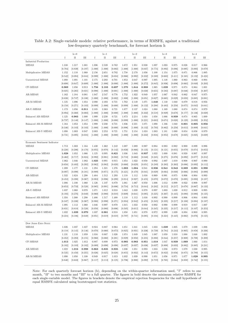
Table A.2: Single-variable models: relative performance, in terms of RMSFE, against a traditionallow-frequency quarterly benchmark, for forecast horizon h

h=0 h=1 h=2 h=3 h=4


Industrial Production

MIDAS 1.248 1.317 1.001 1.896 2.539 0.762 1.672 1.951 0.930 1.097 1.093 0.975 0.826 0.817 0.966

[0.784] [0.839] [0.197] [1.000] [1.000] [0.002] [1.000] [1.000] [0.037] [0.774] [0.892] [0.086] [0.095] [0.093] [0.079]


[0.542] [0.094] [0.044] [0.999] [1.000] [0.034] [0.966] [0.992] [0.332] [0.589] [0.603] [0.411] [0.165] [0.132] [0.424]


[0.698] [0.647] [0.609] [1.000] [1.000] [0.000] [1.000] [1.000] [0.272] [0.845] [0.936] [0.696] [0.063] [0.049] [0.203]

CF-MIDAS 0.969 1.056 0.913 1.756 2.183 0.697 1.570 1.844 0.908 1.065 1.039 0.971 0.874 0.864 1.001

[0.025] [0.265] [0.021] [0.998] [1.000] [0.001] [1.000] [1.000] [0.030] [0.655] [0.583] [0.087] [0.046] [0.058] [0.307]

AR-MIDAS 1.162 1.184 0.981 1.947 2.547 0.776 1.752 1.922 0.949 1.057 1.067 0.942 0.862 0.847 0.975

[0.838] [0.747] [0.100] [1.000] [1.000] [0.002] [1.000] [1.000] [0.051] [0.627] [0.665] [0.029] [0.033] [0.085] [0.081]

AR-M-MIDAS 1.125 1.096 1.054 2.090 2.493 0.721 1.762 2.149 1.071 1.040 1.140 1.040 0.879 0.818 0.956

[0.158] [0.271] [0.103] [0.999] [1.000] [0.000] [0.999] [1.000] [0.132] [0.288] [0.483] [0.250] [0.075] [0.043] [0.041]

AR-U-MIDAS 1.173 1.056 0.911 2.105 2.363 0.721 1.877 2.137 1.024 1.080 1.169 1.080 0.874 0.874 0.979

[0.894] [0.368] [0.003] [1.000] [1.000] [0.000] [1.000] [1.000] [0.332] [0.518] [0.929] [0.678] [0.177] [0.136] [0.029]


[0.737] [0.140] [0.147] [1.000] [1.000] [0.000] [0.999] [1.000] [0.221] [0.683] [0.674] [0.028] [0.129] [0.099] [0.352]


[0.346] [0.103] [0.103] [1.000] [1.000] [0.000] [0.996] [1.000] [0.132] [0.793] [0.862] [0.250] [0.013] [0.009] [0.041]


[0.731] [0.095] [0.016] [1.000] [1.000] [0.000] [1.000] [1.000] [0.332] [0.916] [0.953] [0.678] [0.025] [0.025] [0.029]

Economic Sentiment Indicator

MIDAS 1.713 1.303 1.164 1.430 1.362 1.242 1.087 1.089 0.987 0.984 0.983 0.982 0.900 0.899 0.996

[0.220] [0.206] [0.170] [0.955] [0.978] [0.142] [0.830] [0.866] [0.135] [0.121] [0.121] [0.055] [0.079] [0.074] [0.053]


[0.462] [0.717] [0.824] [0.992] [0.981] [0.002] [0.710] [0.660] [0.040] [0.245] [0.275] [0.076] [0.092] [0.077] [0.212]


[0.658] [0.402] [0.392] [0.962] [0.982] [0.020] [0.660] [0.629] [0.051] [0.249] [0.383] [0.363] [0.086] [0.092] [0.112]

CF-MIDAS 1.209 1.177 1.131 1.294 1.321 1.276 1.003 1.004 0.941 0.936 0.941 0.943 0.889 0.891 0.990

[0.097] [0.098] [0.181] [0.909] [0.971] [0.175] [0.421] [0.470] [0.041] [0.029] [0.064] [0.030] [0.066] [0.083] [0.099]

AR-MIDAS 1.532 1.624 1.298 1.484 1.512 1.293 1.110 1.112 1.016 0.969 0.991 0.975 0.906 0.904 0.993

[0.453] [0.398] [0.367] [0.983] [0.996] [0.299] [0.914] [0.927] [0.455] [0.070] [0.072] [0.070] [0.095] [0.093] [0.187]

AR-M-MIDAS 1.086 1.100 1.060 1.126 1.107 0.870 1.061 1.067 0.950 1.006 1.012 0.999 0.922 0.909 0.997

[0.653] [0.733] [0.528] [0.985] [0.991] [0.006] [0.734] [0.713] [0.044] [0.202] [0.212] [0.217] [0.078] [0.067] [0.133]

AR-U-MIDAS 1.037 1.068 0.970 1.071 1.012 0.918 1.043 1.039 0.978 0.997 1.003 1.039 0.912 0.909 0.995

[0.193] [0.276] [0.049] [0.969] [0.980] [0.018] [0.609] [0.641] [0.085] [0.225] [0.307] [0.445] [0.080] [0.080] [0.125]


[0.347] [0.330] [0.367] [0.988] [0.990] [0.371] [0.934] [0.942] [0.455] [0.345] [0.335] [0.217] [0.100] [0.094] [0.187]


[0.831] [0.818] [0.528] [0.958] [0.980] [0.006] [0.505] [0.612] [0.044] [0.345] [0.335] [0.217] [0.113] [0.107] [0.353]


[0.224] [0.186] [0.049] [0.951] [0.019] [0.018] [0.797] [0.741] [0.085] [0.104] [0.324] [0.445] [0.062] [0.076] [0.125]

Dow Jones Euro Stoxx

MIDAS 1.026 1.037 1.027 0.924 0.887 0.964 1.051 1.041 1.045 1.033 1.039 1.005 1.079 1.039 1.006

[0.118] [0.145] [0.146] [0.070] [0.068] [0.073] [0.925] [0.931] [0.336] [0.739] [0.784] [0.243] [0.905] [0.858] [0.336]


[0.352] [0.293] [0.155] [0.960] [0.068] [0.201] [0.929] [0.950] [0.355] [0.880] [0.844] [0.257] [0.909] [0.798] [0.209]

CF-MIDAS 1.013 1.025 1.012 0.887 0.899 0.973 0.985 0.983 0.951 1.018 1.047 0.939 1.069 1.060 1.014

[0.102] [0.103] [0.102] [0.089] [0.090] [0.098] [0.037] [0.037] [0.036] [0.637] [0.800] [0.033] [0.882] [0.885] [0.241]

AR-MIDAS 1.022 1.016 0.998 0.863 0.835 0.935 1.036 1.051 0.993 1.033 1.056 0.973 1.079 1.030 0.995

[0.535] [0.450] [0.355] [0.026] [0.025] [0.028] [0.855] [0.932] [0.143] [0.672] [0.822] [0.056] [0.875] [0.789] [0.155]

AR-M-MIDAS 1.090 1.050 1.108 0.949 0.917 1.013 1.032 1.039 0.990 1.051 1.056 0.971 1.077 1.028 0.995

[0.840] [0.633] [0.867] [0.117] [0.113] [0.125] [0.796] [0.908] [0.092] [0.719] [0.765] [0.044] [0.859] [0.742] [0.155]

Note: For each quarterly forecast horizon (h), depending on the within-quarter information used, ”I” refers to onemonth, ”II” to two months and ”III” to a full quarter. The figures in bold denote the minimum relative RMSFE foreach single-variable model. The figures in brackets denote the empirical rejection frequencies for the null hypothesis ofequal RMSFE calculated using bootstrapped test statistics.

25

Banco de Portugal | Working Papers i

WORKING PAPERS

2010

1/10 MEASURING COMOVEMENT IN THE TIME-FREQUENCY SPACE

— António Rua

2/10 EXPORTS, IMPORTS AND WAGES: EVIDENCE FROM MATCHED FIRM-WORKER-PRODUCT PANELS

— Pedro S. Martins, Luca David Opromolla

3/10 NONSTATIONARY EXTREMES AND THE US BUSINESS CYCLE

— Miguel de Carvalho, K. Feridun Turkman, António Rua

4/10 EXPECTATIONS-DRIVEN CYCLES IN THE HOUSING MARKET

— Luisa Lambertini, Caterina Mendicino, Maria Teresa Punzi

5/10 COUNTERFACTUAL ANALYSIS OF BANK MERGERS

— Pedro P. Barros, Diana Bonfi m, Moshe Kim, Nuno C. Martins

6/10 THE EAGLE. A MODEL FOR POLICY ANALYSIS OF MACROECONOMIC INTERDEPENDENCE IN THE EURO AREA

— S. Gomes, P. Jacquinot, M. Pisani

7/10 A WAVELET APPROACH FOR FACTOR-AUGMENTED FORECASTING

— António Rua

8/10 EXTREMAL DEPENDENCE IN INTERNATIONAL OUTPUT GROWTH: TALES FROM THE TAILS

— Miguel de Carvalho, António Rua

9/10 TRACKING THE US BUSINESS CYCLE WITH A SINGULAR SPECTRUM ANALYSIS

— Miguel de Carvalho, Paulo C. Rodrigues, António Rua

10/10 A MULTIPLE CRITERIA FRAMEWORK TO EVALUATE BANK BRANCH POTENTIAL ATTRACTIVENESS

— Fernando A. F. Ferreira, Ronald W. Spahr, Sérgio P. Santos, Paulo M. M. Rodrigues

11/10 THE EFFECTS OF ADDITIVE OUTLIERS AND MEASUREMENT ERRORS WHEN TESTING FOR STRUCTURAL BREAKS

IN VARIANCE

— Paulo M. M. Rodrigues, Antonio Rubia

12/10 CALENDAR EFFECTS IN DAILY ATM WITHDRAWALS

— Paulo Soares Esteves, Paulo M. M. Rodrigues

13/10 MARGINAL DISTRIBUTIONS OF RANDOM VECTORS GENERATED BY AFFINE TRANSFORMATIONS OF

INDEPENDENT TWO-PIECE NORMAL VARIABLES

— Maximiano Pinheiro

14/10 MONETARY POLICY EFFECTS: EVIDENCE FROM THE PORTUGUESE FLOW OF FUNDS

— Isabel Marques Gameiro, João Sousa

15/10 SHORT AND LONG INTEREST RATE TARGETS

— Bernardino Adão, Isabel Correia, Pedro Teles

16/10 FISCAL STIMULUS IN A SMALL EURO AREA ECONOMY

— Vanda Almeida, Gabriela Castro, Ricardo Mourinho Félix, José Francisco Maria

17/10 FISCAL INSTITUTIONS AND PUBLIC SPENDING VOLATILITY IN EUROPE

— Bruno Albuquerque

Banco de Portugal | Working Papers ii

18/10 GLOBAL POLICY AT THE ZERO LOWER BOUND IN A LARGE-SCALE DSGE MODEL

— S. Gomes, P. Jacquinot, R. Mestre, J. Sousa

19/10 LABOR IMMOBILITY AND THE TRANSMISSION MECHANISM OF MONETARY POLICY IN A MONETARY UNION

— Bernardino Adão, Isabel Correia

20/10 TAXATION AND GLOBALIZATION

— Isabel Correia

21/10 TIME-VARYING FISCAL POLICY IN THE U.S.

— Manuel Coutinho Pereira, Artur Silva Lopes

22/10 DETERMINANTS OF SOVEREIGN BOND YIELD SPREADS IN THE EURO AREA IN THE CONTEXT OF THE ECONOMIC

AND FINANCIAL CRISIS

— Luciana Barbosa, Sónia Costa

23/10 FISCAL STIMULUS AND EXIT STRATEGIES IN A SMALL EURO AREA ECONOMY


24/10 FORECASTING INFLATION (AND THE BUSINESS CYCLE?) WITH MONETARY AGGREGATES

— João Valle e Azevedo, Ana Pereira

25/10 THE SOURCES OF WAGE VARIATION: AN ANALYSIS USING MATCHED EMPLOYER-EMPLOYEE DATA

— Sónia Torres,Pedro Portugal, John T.Addison, Paulo Guimarães

26/10 THE RESERVATION WAGE UNEMPLOYMENT DURATION NEXUS

— John T. Addison, José A. F. Machado, Pedro Portugal

27/10 BORROWING PATTERNS, BANKRUPTCY AND VOLUNTARY LIQUIDATION

— José Mata, António Antunes, Pedro Portugal

28/10 THE INSTABILITY OF JOINT VENTURES: LEARNING FROM OTHERS OR LEARNING TO WORK WITH OTHERS

— José Mata, Pedro Portugal

29/10 THE HIDDEN SIDE OF TEMPORARY EMPLOYMENT: FIXED-TERM CONTRACTS AS A SCREENING DEVICE

— Pedro Portugal, José Varejão

30/10 TESTING FOR PERSISTENCE CHANGE IN FRACTIONALLY INTEGRATED MODELS: AN APPLICATION TO WORLD

INFLATION RATES

— Luis F. Martins, Paulo M. M. Rodrigues

31/10 EMPLOYMENT AND WAGES OF IMMIGRANTS IN PORTUGAL

— Sónia Cabral, Cláudia Duarte

32/10 EVALUATING THE STRENGTH OF IDENTIFICATION IN DSGE MODELS. AN A PRIORI APPROACH

— Nikolay Iskrev

33/10 JOBLESSNESS

— José A. F. Machado, Pedro Portugal, Pedro S. Raposo

2011

1/11 WHAT HAPPENS AFTER DEFAULT? STYLIZED FACTS ON ACCESS TO CREDIT

— Diana Bonfi m, Daniel A. Dias, Christine Richmond

2/11 IS THE WORLD SPINNING FASTER? ASSESSING THE DYNAMICS OF EXPORT SPECIALIZATION

— João Amador

Banco de Portugal | Working Papers iii

3/11 UNCONVENTIONAL FISCAL POLICY AT THE ZERO BOUND

— Isabel Correia, Emmanuel Farhi, Juan Pablo Nicolini, Pedro Teles

4/11 MANAGERS’ MOBILITY, TRADE STATUS, AND WAGES

— Giordano Mion, Luca David Opromolla

5/11 FISCAL CONSOLIDATION IN A SMALL EURO AREA ECONOMY


6/11 CHOOSING BETWEEN TIME AND STATE DEPENDENCE: MICRO EVIDENCE ON FIRMS’ PRICE-REVIEWING

STRATEGIES

— Daniel A. Dias, Carlos Robalo Marques, Fernando Martins

7/11 WHY ARE SOME PRICES STICKIER THAN OTHERS? FIRM-DATA EVIDENCE ON PRICE ADJUSTMENT LAGS

— Daniel A. Dias, Carlos Robalo Marques, Fernando Martins, J. M. C. Santos Silva

8/11 LEANING AGAINST BOOM-BUST CYCLES IN CREDIT AND HOUSING PRICES

— Luisa Lambertini, Caterina Mendicino, Maria Teresa Punzi

9/11 PRICE AND WAGE SETTING IN PORTUGAL LEARNING BY ASKING

— Fernando Martins

10/11 ENERGY CONTENT IN MANUFACTURING EXPORTS: A CROSS-COUNTRY ANALYSIS

— João Amador

11/11 ASSESSING MONETARY POLICY IN THE EURO AREA: A FACTOR-AUGMENTED VAR APPROACH

— Rita Soares

12/11 DETERMINANTS OF THE EONIA SPREAD AND THE FINANCIAL CRISIS

— Carla Soares, Paulo M. M. Rodrigues

13/11 STRUCTURAL REFORMS AND MACROECONOMIC PERFORMANCE IN THE EURO AREA COUNTRIES: A MODEL-

BASED ASSESSMENT

— S. Gomes, P. Jacquinot, M. Mohr, M. Pisani

14/11 RATIONAL VS. PROFESSIONAL FORECASTS

— João Valle e Azevedo, João Tovar Jalles

15/11 ON THE AMPLIFICATION ROLE OF COLLATERAL CONSTRAINTS

— Caterina Mendicino

16/11 MOMENT CONDITIONS MODEL AVERAGING WITH AN APPLICATION TO A FORWARD-LOOKING MONETARY

POLICY REACTION FUNCTION

— Luis F. Martins

17/11 BANKS’ CORPORATE CONTROL AND RELATIONSHIP LENDING: EVIDENCE FROM RETAIL LOANS

— Paula Antão, Miguel A. Ferreira, Ana Lacerda

18/11 MONEY IS AN EXPERIENCE GOOD: COMPETITION AND TRUST IN THE PRIVATE PROVISION OF MONEY

— Ramon Marimon, Juan Pablo Nicolini, Pedro Teles

19/11 ASSET RETURNS UNDER MODEL UNCERTAINTY: EVIDENCE FROM THE EURO AREA, THE U.K. AND THE U.S.

— João Sousa, Ricardo M. Sousa

20/11 INTERNATIONAL ORGANISATIONS’ VS. PRIVATE ANALYSTS’ FORECASTS: AN EVALUATION

— Ildeberta Abreu

21/11 HOUSING MARKET DYNAMICS: ANY NEWS?

— Sandra Gomes, Caterina Mendicino

Banco de Portugal | Working Papers iv

22/11 MONEY GROWTH AND INFLATION IN THE EURO AREA: A TIME-FREQUENCY VIEW

— António Rua

23/11 WHY EX(IM)PORTERS PAY MORE: EVIDENCE FROM MATCHED FIRM-WORKER PANELS

— Pedro S. Martins, Luca David Opromolla

24/11 THE IMPACT OF PERSISTENT CYCLES ON ZERO FREQUENCY UNIT ROOT TESTS

— Tomás del Barrio Castro, Paulo M.M. Rodrigues, A.M. Robert Taylor

25/11 THE TIP OF THE ICEBERG: A QUANTITATIVE FRAMEWORK FOR ESTIMATING TRADE COSTS

— Alfonso Irarrazabal, Andreas Moxnes, Luca David Opromolla

26/11 A CLASS OF ROBUST TESTS IN AUGMENTED PREDICTIVE REGRESSIONS

— Paulo M.M. Rodrigues, Antonio Rubia

27/11 THE PRICE ELASTICITY OF EXTERNAL DEMAND: HOW DOES PORTUGAL COMPARE WITH OTHER EURO AREA

COUNTRIES?

— Sónia Cabral, Cristina Manteu

28/11 MODELING AND FORECASTING INTERVAL TIME SERIES WITH THRESHOLD MODELS: AN APPLICATION TO

S&P500 INDEX RETURNS

— Paulo M. M. Rodrigues, Nazarii Salish

29/11 DIRECT VS BOTTOM-UP APPROACH WHEN FORECASTING GDP: RECONCILING LITERATURE RESULTS WITH

INSTITUTIONAL PRACTICE

— Paulo Soares Esteves

30/11 A MARKET-BASED APPROACH TO SECTOR RISK DETERMINANTS AND TRANSMISSION IN THE EURO AREA

— Martín Saldías

31/11 EVALUATING RETAIL BANKING QUALITY SERVICE AND CONVENIENCE WITH MCDA TECHNIQUES: A CASE

STUDY AT THE BANK BRANCH LEVEL

— Fernando A. F. Ferreira, Sérgio P. Santos, Paulo M. M. Rodrigues, Ronald W. Spahr

2012

1/12 PUBLIC-PRIVATE WAGE GAPS IN THE PERIOD PRIOR TO THE ADOPTION OF THE EURO: AN APPLICATION

BASED ON LONGITUDINAL DATA

— Maria Manuel Campos, Mário Centeno

2/12 ASSET PRICING WITH A BANK RISK FACTOR

— João Pedro Pereira, António Rua

3/12 A WAVELET-BASED ASSESSMENT OF MARKET RISK: THE EMERGING MARKETS CASE

— António Rua, Luis C. Nunes

4/12 COHESION WITHIN THE EURO AREA AND THE U. S.: A WAVELET-BASED VIEW

— António Rua, Artur Silva Lopes

5/12 EXCESS WORKER TURNOVER AND FIXED-TERM CONTRACTS: CAUSAL EVIDENCE IN A TWO-TIER SYSTEM

— Mário Centeno, Álvaro A. Novo

6/12 THE DYNAMICS OF CAPITAL STRUCTURE DECISIONS

— Paula Antão, Diana Bonfi m

7/12 QUANTILE REGRESSION FOR LONG MEMORY TESTING: A CASE OF REALIZED VOLATILITY

— Uwe Hassler, Paulo M. M. Rodrigues, Antonio Rubia

Banco de Portugal | Working Papers v

8/12 COMPETITION IN THE PORTUGUESE ECONOMY: AN OVERVIEW OF CLASSICAL INDICATORS

— João Amador, Ana Cristina Soares

9/12 MARKET PERCEPTION OF FISCAL SUSTAINABILITY: AN APPLICATION TO THE LARGEST EURO AREA ECONOMIES

— Maximiano Pinheiro

10/12 THE EFFECTS OF PUBLIC SPENDING EXTERNALITIES

— Valerio Ercolani, João Valle e Azevedo

11/12 COLLATERAL REQUIREMENTS: MACROECONOMIC FLUCTUATIONS AND MACRO-PRUDENTIAL POLICY

— Caterina Mendicino

12/12 WAGE RIGIDITY AND EMPLOYMENT ADJUSTMENT AT THE FIRM LEVEL: EVIDENCE FROM SURVEY DATA


13/12 HOW TO CREATE INDICES FOR BANK BRANCH FINANCIAL PERFORMANCE MEASUREMENT USING MCDA

TECHNIQUES: AN ILLUSTRATIVE EXAMPLE

— Fernando A. F. Ferreira, Paulo M. M. Rodrigues, Sérgio P. Santos, Ronald W. Spahr

14/12 ON INTERNATIONAL POLICY COORDINATION AND THE CORRECTION OF GLOBAL IMBALANCES

— Bruno Albuquerque, Cristina Manteu

15/12 IDENTIFYING THE DETERMINANTS OF DOWNWARD WAGE RIGIDITY: SOME METHODOLOGICAL

CONSIDERATIONS AND NEW EMPIRICAL EVIDENCE


16/12 SYSTEMIC RISK ANALYSIS USING FORWARD-LOOKING DISTANCE-TO-DEFAULT SERIES

— Martín Saldías

17/12 COMPETITION IN THE PORTUGUESE ECONOMY: INSIGHTS FROM A PROFIT ELASTICITY APPROACH


18/12 LIQUIDITY RISK IN BANKING: IS THERE HERDING?

— Diana Bonfi m, Moshe Kim

19/12 BANK SIZE AND LENDING SPECIALIZATION

— Diana Bonfi m, Qinglei Dai

2013

01/13 MACROECONOMIC FORECASTING USING LOW-FREQUENCY FILTERS

— João Valle e Azevedo, Ana Pereira

02/13 EVERYTHING YOU ALWAYS WANTED TO KNOW ABOUT SEX DISCRIMINATION

— Ana Rute Cardoso, Paulo Guimarães, Pedro Portugal

03/13 IS THERE A ROLE FOR DOMESTIC DEMAND PRESSURE ON EXPORT PERFORMANCE?

— Paulo Soares Esteves, António Rua

04/13 AGEING AND FISCAL SUSTAINABILITY IN A SMALL EURO AREA ECONOMY

— Gabriela Castro, José R. Maria, Ricardo Mourinho Félix, Cláudia Rodrigues Braz

05/13 MIND THE GAP! THE RELATIVE WAGES OF IMMIGRANTS IN THE PORTUGUESE LABOUR MARKET

— Sónia Cabral, Cláudia Duarte

06/13 FOREIGN DIRECT INVESTMENT AND INSTITUTIONAL REFORM: EVIDENCE AND AN APPLICATION TO PORTUGAL

— Paulo Júlio, Ricardo Pinheiro-Alves, José Tavares

Banco de Portugal | Working Papers vi

07/13 MONETARY POLICY SHOCKS: WE GOT NEWS!

— Sandra Gomes, Nikolay Iskrev, Caterina Mendicino

08/13 COMPETITION IN THE PORTUGUESE ECONOMY: ESTIMATED PRICE-COST MARGINS UNDER IMPERFECT

LABOUR MARKETS


09/13 THE SOURCES OF WAGE VARIATION: A THREE-WAY HIGH-DIMENSIONAL FIXED EFFECTS REGRESSION MODEL

— Sonia Torres, Pedro Portugal , John T. Addison, Paulo Guimarães

10/13 THE OUTPUT EFFECTS OF (NON-SEPARABLE) GOVERNMENT CONSUMPTION AT THE ZERO LOWER BOUND

— Valerio Ercolani, João Valle e Azevedo

11/13 FISCAL MULTIPLIERS IN A SMALL EURO AREA ECONOMY: HOW BIG CAN THEY GET IN CRISIS TIMES?

— Gabriela Castro, Ricardo M. Felix, Paulo Julio, Jose R. Maria

12/13 SURVEY EVIDENCE ON PRICE AND WAGE RIGIDITIES IN PORTUGAL

— Fernando Martins

13/13 CHARACTERIZING ECONOMIC GROWTH PATHS BASED ON NEW STRUCTURAL CHANGE TESTS

— Nuno Sobreira, Luis C. Nunes, Paulo M. M. Rodrigues

14/13 CATASTROPHIC JOB DESTRUCTION

— Anabela Carneiro, Pedro Portugal, José Varejão

15/13 OUTPUT EFFECTS OF A MEASURE OF TAX SHOCKS BASED ON CHANGES IN LEGISLATION FOR PORTUGAL

— Manuel Coutinho Pereira, Lara Wemans

16/13 INSIDE PESSOA - A DETAILED DESCRIPTION OF THE MODEL

— Vanda Almeida, Gabriela Castro, Ricardo M. Félix, Paulo Júlio, José R. Maria

17/13 MACROPRUDENTIAL REGULATION AND MACROECONOMIC ACTIVITY

— Sudipto Karmakar

18/13 BANK CAPITAL AND LENDING: AN ANALYSIS OF COMMERCIAL BANKS IN THE UNITED STATES

— Sudipto Karmakar, Junghwan Mok

2014

1/14 AUTOREGRESSIVE AUGMENTATION OF MIDAS REGRESSIONS

— Cláudia Duarte

AUTOREGRESSIVE AUGMENTATION OF MIDAS REGRESSIONS · MIDAS regressions see Andreou et al., 2011)....

Documents

Transcript of AUTOREGRESSIVE AUGMENTATION OF MIDAS REGRESSIONS · MIDAS regressions see Andreou et al., 2011)....