Size Effect on Fatigue Crack Growth of a Quasibrittle

Material

A THESIS

SUBMITTED TO THE FACULTY OF THE GRADUATE SCHOOL

OF THE UNIVERSITY OF MINNESOTA

BY

Jonathan Manning

IN PARTIAL FULFILLMENT OF THE REQUIREMENTS

FOR THE DEGREE OF

MASTER OF SCIENCE

Professors Joseph F. Labuz and Jia-Liang Le

January 2013

i

Abstract

The Paris-Erdogan law describes the rate of fatigue crack growth as a function

of the amplitude of the applied stress intensity factor. This equation, however, does not

include a dependence of the crack growth on the structure size, which has been

observed experimentally for concrete. The size effect on the fatigue crack growth is

derived based on two hypotheses: (1) the scaling of the critical energy dissipation for

fatigue crack growth has the same form as that of fracture energy for monotonic

loading; (2) the difference in transitional sizes between the fatigue and monotonic

loading is purely due to the difference in the fracture process zone (FPZ) size. The size-

dependent fatigue crack growth law is verified experimentally through size effect tests

on Berea sandstone. Using digital image correlation, it is shown that the FPZ length is

approximately 7 mm and 11 mm for monotonic and cyclic loading, respectively.

Optimal fitting resulted in transitional sizes of 34 mm and 54 mm for monotonic

loading and cyclic loading, respectively, which shows a proportional relationship

between the FPZ length and the transitional size.

ii

Table of Contents

List of Tables……………………………………………………………………. iii

List of Figures…………………………………………………………………… iv

1.0 Introduction…………………………………………………………………. 1

1.1 Motivation………………………………………………………………….. 1

1.2 Objective……………………………………………………………………. 2

1.3 Scope and Organization…………………………………………………….. 2

2.0 Background ………………….……………………………………………… 3

2.1 Fracture and Fatigue………………………………………………………… 3

2.2 Size Effect on Nominal Strength……….…………………………………… 4

2.3 Fracture Process Zone………………………………………………………. 6

2.4 Digital Image Correlation….………………..……………………..………... 8

3.0 Fatigue Crack Growth – Theoretical Framework………………………….. 12

3.1 Fatigue Crack Growth at the Large-size Limit…...…………………………. 10

3.2 Scaling of Fatigue Crack Growth Law………..…………………..………… 15

4.0 Monotonic Size Effect Test…..……………………………………………... 17

4.1 Experimental Setup…………………………………………………………. 17

4.2 Nominal Strength Calculation………………………………………………. 18

4.3 Fracture Properties from Size Effect Analysis……………………………… 22

4.4 Fracture Process Zone Length – Monotonic Loading………………………. 25

4.5 Displacement Gradient Method for Tracking FPZ…………………………. 35

5.0 Fatigue Crack Growth Size Effect Test………...……………………………… 40

5.1 Experimental Setup…………………..……………………………………... 41

5.2 Compliance Calibration Method……………………………………………. 43

5.3 Paris-Erdogan Law calculated from Compliance Method………………….. 41

5.4 Fracture Process Zone Length – Cyclic Loading …………………………... 51

5.5 Paris-Erdogan Law Calculated from DIC Method………………………….. 56

6.0 Conclusions……………………………………………………...…………………. 62

7.0 References………………………………………………………………………….. 64

iii

List of Tables

4.1 Specimen properties for monotonic loading……………………………………. 19

4.2 Average nominal strength………………………………………………………. 19

4.3 Fracture parameter for Berea sandstone………………………………………… 23

4.4 Displacement gradient at tip of FPZ for a medium sized specimen…………….. 37

5.1 Specimen properties for cyclic loading…………………………………………. 40

5.2 Young’s Modulus used to calibrate CMOD compliance curves………………… 43

5.3 Cycles analyzed for Paris-Erdogan Law………………………………………… 47

5.4 Fracture process zone lengths for all four specimens……………………... 56

5.5 Cycles where the FPZ tip increases by 1 mm for specimen 2-4……………….... 57

iv

List of Figures

2.1 Size effect results for various rocks and ceramics……………………………….. 5

2.2 Fracture process zone schematic…………………………………………………. 6

2.3 Locations of acoustic emission at peak load…………………………………...... 7

2.4 Digital image of a painted specimen…………….……………………………..... 9

2.5 Schematic of DIC process……………………….……………………………..... 11

3.1 Cyclic FPZ composed of many micro-cracks…….……………………………… 13

4.1 Specimen geometry for three-point bending experiments...……………………… 17

4.2 Experimental setup ………………………………………………………………. 18

4.3 Load vs. CMOD for small specimens……………………………………………. 19

4.4 Load vs. CMOD for medium specimens…………………………………………. 20

4.5 Load vs. CMOD for large specimens….…………………………………………. 20

4.6 Nominal strength vs. CMOD for one specimen of each size…………………….. 21

4.7 Linear regression of experimental results………………………………………… 23

4.8 Size effect of nominal strength…………………………………………………… 24

4.9 Horizontal displ. contours – medium specimen – 30% to 40% peak load………. 25

4.10 Horizontal displ. measurements along horizontal lines – 30% to 40% peak……. 26

4.11 Horizontal displ. contours – medium specimen – 60% to 70% peak load………. 27

4.12 Horizontal displ. measurements along horizontal lines – 60% to 70% peak …… 28

4.13 Horizontal displ. contours – medium specimen – 90% to 100% peak load……… 29

4.14 Horizontal displ. contours – medium specimen – 100% to 90% post-peak load… 30

4.15 Post peak fracture process zone vs. traction free surface – medium specimens…. 31

4.16 Horizontal displ. contours – large specimen – 95% to 100% peak load………… 32

4.17 Horizontal displ. contours – large specimen – 100% to 95% post-peak load…… 28

4.18 Post peak fracture process zone vs. traction free surface – large specimens…….. 33

4.19 Post peak fracture process zone vs. traction free surface – small specimens……. 34

4.20 Displacement gradient vs. distance from the notch tip…………………………... 36

4.21 Displacement gradient calculation……………………………………………….. 37

4.22 Displacement gradient at tip vs. incremental CMOD – medium specimen……... 38

4.23 Displacement gradient contours for a medium specimen………………………... 38

4.24 Displacement gradient at tip vs. incremental CMOD – large specimen………… 39

4.25 Displacement gradient contours for a large specimen…………………………… 39

v

5.1 Load vs. time for cyclic 3-point bending tests…………………………………… 40

5.2 Zoomed in view of CMOD gage, Numerical analysis…………………………… 41

5.3 CMOD vs. Effective crack length ratio……………………….…………………. 42

5.4 Load vs. CMOD for different cycles…………………………………………….. 44

5.5 Peak and valley CMOD measurements vs. cycles………………………………. 44

5.6 Effective crack evolution vs. cycles……………………………………………... 45

5.7 da/dN vs. ΔK for medium specimen…………………………………………….. 46

5.8 Effective crack vs. cycles for specimen 2-5, showing stages of crack growth….. 47

5.9 Paris-Erdogan law for all four specimens plotted individually…………………. 48

5.10 Paris-Erdogan law for all three sizes with a fixed slope……………………….... 48

5.11 Size-dependent Paris-Erdogan law using D0 = 34mm…………………………... 50

5.12 Size-dependent Paris-Erdogan law using D0 = 54mm………………………….. 50

5.13 Horizontal displacement contours – medium specimen – cycle 6,000………….. 52

5.14 Horizontal displacement contours – medium specimen – cycle 13,900………… 53

5.15 Horizontal displacement contours – large specimen – cycle 12,000……………. 54

5.16 Horizontal displacement contours – large specimen – cycle 20,500……………. 54

5.17 Horizontal displacement contours – large specimen – cycle 21,600……………. 55

5.18 Horizontal displacement contours – medium specimen – cycle 2………………. 57

5.19 Effective crack ratio vs. cycles computed using DIC method…………………... 58

5.20 da/dN vs. ΔK calculated form DIC method for medium specimen 2-5…………. 59

5.21 da/dN vs. ΔK calculated form DIC method for large specimen 3-4…………….. 60

5.22 da/dN vs. ΔK calculated form DIC for all four specimens……………………… 60

5.23 Size-dependent Paris-Erdogan law applied to DIC results with D0 = 47mm…… 61

1

Chapter 1: Introduction

1.1 Motivation

In many fields of engineering, the designed products will be exposed to repeated

loading, i.e., cars driving over a bridge, gas expanding and contracting inside a vessel, or

weight being applied to a prosthetic leg when walking. Understanding how these

structures behave through time is of great interest in determining the safety of an aging

structure.

Geoengineering is a challenging field because the natural material within the earth

has a high degree of variability. However difficult, the expectations for safety and

reliability remain the same for structures built within the earth, i.e., tunnels, underground

buildings or oil pipe lines. Great works have been constructed in the field of

geoengineering in the past century, but many phenomena are still not completely

understood, and one of such fields is fatigue. Very few studies have focused on fatigue in

rock materials, and very little is published to explain the lifespan predictions of

geological structures that are exposed to cyclic loading.

This research is focused on investigating fatigue, specifically, subcritical crack

growth under cyclic loading in a rock. Understanding this phenomenon in greater detail

will provide a better means to design geological structures and predict a more accurate

lifespan.

2

1.2 Objective

The main objectives of the research are to:

Develop a size-dependent Paris-Erdogan equation

Determine the size effect on nominal strength and fracture properties from

monotonic three-point bending experiments

Investigate the validity of the size dependent Paris-Erdogan law by performing

cyclic three-point bending experiments

Compare the fracture process zone length under monotonic loading and cyclic

loading using digital image correlation

1.3 Scope and Organization

This thesis considers the classical Paris-Erdogan law and proposes a size-

dependent version. The thesis is organized into five chapters. Chapter 2 presents a brief

literature review of fatigue, size effect and the experimental technique called digital

image correlation. Chapter 3 discusses the size effect for the Paris-Erdogan law and

proposes a size dependent equation. Chapter 4 presents results from monotonic three-

point bending experiments that are used to determine the size effect of the nominal

strength and the fracture properties. The fracture process zone during monotonic loading

is also investigated using digital image correlation. Chapter 5 presents the results of

cyclic three-point bending experiments. The Paris-Erdogan law is computed as well as

the size-dependent version that is proposed in Chapter 3. The fracture process zone

under cyclic loading is also investigated. Chapter 6 presents a summary of the findings

and conclusions.

3

Chapter 2: Background

2.1 Fracture and Fatigue

Fatigue has been of interest for many years and the expression dates back to the

1800’s when it was used to explain the straining of masts on large sea vessels. The first

known study of fatigue was performed on metals around 1829 by W.A.J Albert, a

German mining engineer, who performed experiments on chains made of iron [1].

During the 1840’s, as larger infrastructure (bridges, railways, etc.) became more popular,

the study of fatigue began to expand [2, 3] and continued into the 20th

century, with many

studies focused on iron railways [4, 5].

Fracture mechanics began with the ground-breaking work of Inglis (1913) and

Griffith (1921), who provided a mathematical approach based on stress analysis and

energy balance [6, 7]. The work laid the foundation for the modern field of linear elastic

fracture mechanics (LEFM) that is largely responsible for the reliability and safety of

bridges, buildings, aircraft, etc. Irwin (1957) expanded on the work and introduced the

term stress intensity factor to quantify the near tip stress field for a crack in a linear

elastic body [8]. The initiation of a “linear elastic” crack, under monotonic loading

conditions, is characterized by a critical value of the stress intensity factor, Kc. This

value is typically classified further by the opening mode where, KIc is the critical stress

intensity factor under mode I separation (tensile opening). This value, KIc, is also

referred to as the fracture toughness of the material.

This approach to fracture was adapted for fatigue by Paris et al. [9] and Paris and

Erdogan [10] by relating the crack growth rate to the change in stress intensity factor

from maximum to minimum load. In the most general form, the Paris-Erdogan law is

( )

, (2.1)

where a = crack length, N = number of cycles, ΔKI = amplitude of stress intensity factor

calculated from linear fracture mechanics, and C and m are both empirical constants.

Paris & Erdogan performed experiments on aluminum alloys with different geometries to

test the law and found that it was consistent for many different combinations of stress

4

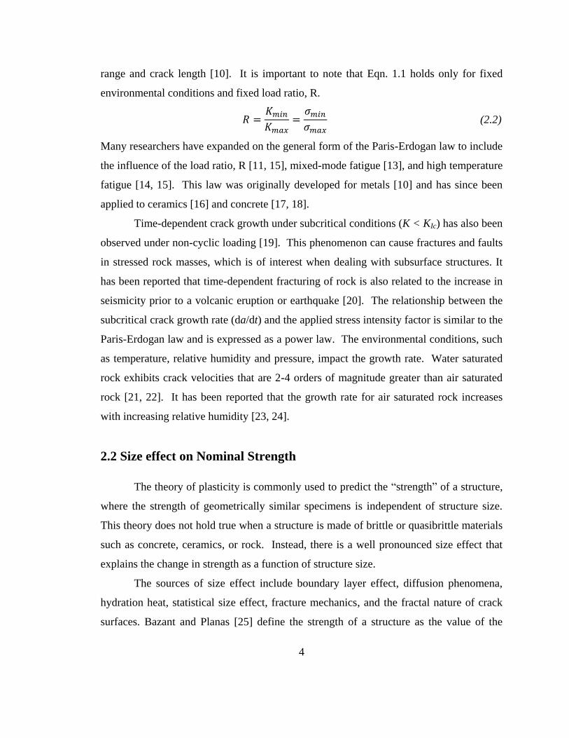
range and crack length [10]. It is important to note that Eqn. 1.1 holds only for fixed

environmental conditions and fixed load ratio, R.

(2.2)

Many researchers have expanded on the general form of the Paris-Erdogan law to include

the influence of the load ratio, R [11, 15], mixed-mode fatigue [13], and high temperature

fatigue [14, 15]. This law was originally developed for metals [10] and has since been

applied to ceramics [16] and concrete [17, 18].

Time-dependent crack growth under subcritical conditions (K < KIc) has also been

observed under non-cyclic loading [19]. This phenomenon can cause fractures and faults

in stressed rock masses, which is of interest when dealing with subsurface structures. It

has been reported that time-dependent fracturing of rock is also related to the increase in

seismicity prior to a volcanic eruption or earthquake [20]. The relationship between the

subcritical crack growth rate (da/dt) and the applied stress intensity factor is similar to the

Paris-Erdogan law and is expressed as a power law. The environmental conditions, such

as temperature, relative humidity and pressure, impact the growth rate. Water saturated

rock exhibits crack velocities that are 2-4 orders of magnitude greater than air saturated

rock [21, 22]. It has been reported that the growth rate for air saturated rock increases

with increasing relative humidity [23, 24].

2.2 Size effect on Nominal Strength

The theory of plasticity is commonly used to predict the “strength” of a structure,

where the strength of geometrically similar specimens is independent of structure size.

This theory does not hold true when a structure is made of brittle or quasibrittle materials

such as concrete, ceramics, or rock. Instead, there is a well pronounced size effect that

explains the change in strength as a function of structure size.

The sources of size effect include boundary layer effect, diffusion phenomena,

hydration heat, statistical size effect, fracture mechanics, and the fractal nature of crack

surfaces. Bazant and Planas [25] define the strength of a structure as the value of the

5

nominal stress at peak load, which is a parameter that is proportional to the load divided

by a cross-sectional area

(2.3)

where P = applied load, b = thickness of a two-dimensional structure and D =

characteristic dimension of the structure. For quasibrittle structures, the nominal strength

varies from a plastic limit for very small structures to a linear elastic fracture mechanics

(LEFM) limit characterized by a slope of -1/2. Through analysis of the energy required

for crack growth, Bažant introduced a size effect function that bridges the two limits,

plasticity and LEFM, and only depends on two parameters:

√ ⁄ (2.4)

where ft’ = tensile strength of the material, B = dimensionless constant and D0 = a

constant with the dimension of length [26]. Figure 2.1 shows the size effect equation

plotted alongside the two limits.

Figure 2.1 – Size Effect Results for various kinds of rocks and ceramics

(Fathy 1992; Bazant, Gettu and Kazemi 1991; McKinney and Rice 1981) [25]

6

2.3 Fracture Process Zone

LEFM predicts infinite stress at a crack tip but in real materials, stresses must

remain finite. As a result, a non-linear zone develops that is composed of a region

characterized by progressive softening and a region characterized by plastic hardening

[25]. For quasibrittle materials, the region of plastic hardening is often negligible and the

majority of the nonlinear zone undergoes softening due to microcracking, crack

deflection, interface breakage, and other phenomena. This zone, commonly called the

fracture process zone (FPZ), is of interest in predicting failure and deciding the

applicability of LEFM.

Figure 2.2 displays a conceptual representation of the FPZ where cohesive

stresses are present within the process zone [27, 28]. The traction inside the process zone

is due to ligaments that remain unbroken as the surfaces separate. Ultimately, the

opening displacement between the two surfaces reaches a critical value, wc, and the

traction becomes zero.

Figure 2.2 – Schematic of the fracture process zone (FPZ) showing the traction free crack and

cohesive tractions that restrict the opening of the FPZ

Cohesive tractions

𝜎

lp

Traction-free crack

7

The length of the FPZ can be written as:

(

)

(2.5)

where η = a dimensionless constant, KIc = mode I fracture toughness and ft = tensile

strength. Irwin estimated the constant, η, by cutting off the LEFM stress field and

placing a limit equal to the yield strength, σY. This concept yields η = 1/π, but stress

redistribution of the plastic (ductile) material is not considered [25].

The FPZ length was observed experimentally by Labuz and Biolzi [29] through

acoustic emission (AE). Transducers, attached to a granite beam, detect acoustic

emissions, which are caused by the development of microcracks. At peak load, the

events localize and provide an estimate for the length and width of the fracture process

zone, as shown in Fig. 2.3. Optical methods, such as speckle interferometry and digital

image correlation, have also been used to measure opening displacements and process

zone lengths in sandstone [30, 31].

Figure 2.3 – Locations of acoustic emission at peak load in a granite beam [47]

8

2.3 Digital Image Correlation

Digital Image Correlation (DIC) is a particle-tracking technique that uses digital

images to generate displacement fields. The technique stemmed from earlier work during

the 1960’s that introduced laser speckles as a tool for observing displacements. The laser

speckle, generated by shining a laser on the surface of a specimen, has a unique size,

shape and intensity that are products of the local microscopic imperfections. When the

specimen deforms, the speckles move and the surface displacement can be tracked by

evaluating the movement of the speckles [32].

Extensive numerical analysis is required to estimate the speckle movement from

the reference image (undeformed surface) to the current image (deformed surface). The

process attempts to track small regions, called subsets, by performing correlation analysis

between the two images [33]. The location of maximum correlation between the

reference image and the current image coincides with the location of the displaced subset.

Many algorithms, with slightly different correlation functions, have been introduced that

use methods such as coarse-fine search [34], Newton-Raphson [35], and Fast Fourier

Transform [36]. Studies have also been focused on analyzing the system error, which can

arise during reconstruction of the intensity patterns [37] and during interpolation in the

approximation of sub-pixel intensity values [38].

The correlation methods have since been applied to many experimental studies.

Peters et al. analyzed rigid body movement using digital correlation methods to calculate

angular velocity and linear velocity of discrete points [39]. Another study, by Chu et al.

deemed the correlation method accurate in the determination of rigid body translations

and rotations [40]. The study also tested the method in a uniform finite-strain test and

found errors to be minimal.

9

2.3.1 DIC Basics

One of the great advantages for using DIC is the ease of setup, which only

requires a camera, lens, image acquisition system, and a software package or code that

can perform the numerical correlation. The camera is setup perpendicular to the

specimen and the lens is focused to create a clear image. The specimen is typically

painted with black and white paint to create speckles. During an experiment, images of

the specimen are taken before and after deformation. The camera converts the light

energy into a digital image that consists of many small squares called pixels. The total

number of pixels per image is commonly called the resolution, which varies depending

on the camera. During the image acquisition process, each pixel is assigned a digital

value, called a grayscale value, which is related to the amount of light energy at that

location. Grayscale values for an eight bit digital image range from 0-255, where

extremely bright (white) pixels have higher grayscale values than dark (black) pixels.

Figure 2.4 – (Left) Digital image of a painted specimen in 3-point bending. (right) Zoomed-in

view of a region of interest (ROI) and a subset used for DIC analysis

Subset

Region of interest

10

Fig. 2.4 displays an image of a specimen with painted speckles that was taken

during a three-point bending experiment. The black region near the middle of the bottom

edge is the notch that is cut into the specimen. The resolution of the image is 1600x1200

pixels and each pixel has a grayscale value from 0-255. There are nearly 2 million pixels

in this image and only 255 different grayscale values, which means there are many pixels

with the same grayscale value. This makes it impossible to track individual pixels.

Instead, groups of pixels, called subsets, are tracked that have a unique pattern of

grayscale values. The size of the subset is set by the user and typically ranges from

20x20 pixels to 128x128 pixels.

The objective is to scan the current image to find the new location of the

displaced subset. Many times the displacements are very small and it is not necessary to

scan the entire image to locate the subset. Instead, the user specifies another parameter,

called the region of interest (ROI), which is a region, many times smaller than the entire

image, where the algorithm scans for the displaced subset. Restricting the scanning area

substantially increases the speed of the correlation process. Fig. 2.4 also shows a

zoomed-in view of a region of interest that is almost four times larger than the subset but

still very small in relation to the entire image.

The DIC software package used for this research is DaVis, which is produced by

LaVision Inc. (Ypsilanti, MI). The package combines the most advanced Fast Fourier

Transform algorithms with the highest quality software to create an easy to use interface

for analysis [41]. Fig. 2.5 shows a schematic of the analysis procedure. The software

recognizes two photos at different times, t1 and t2, and discretizes the image into smaller

cells (subsets). A correlation field between t1 and t2 is computed in each cell using Fast

Fourier Transformation and the maximum correlation corresponds to the displacement.

The software uses multi-pass processing and Whittaker reconstruction to maximize the

sub-pixel accuracy to 0.01 pixels.

11

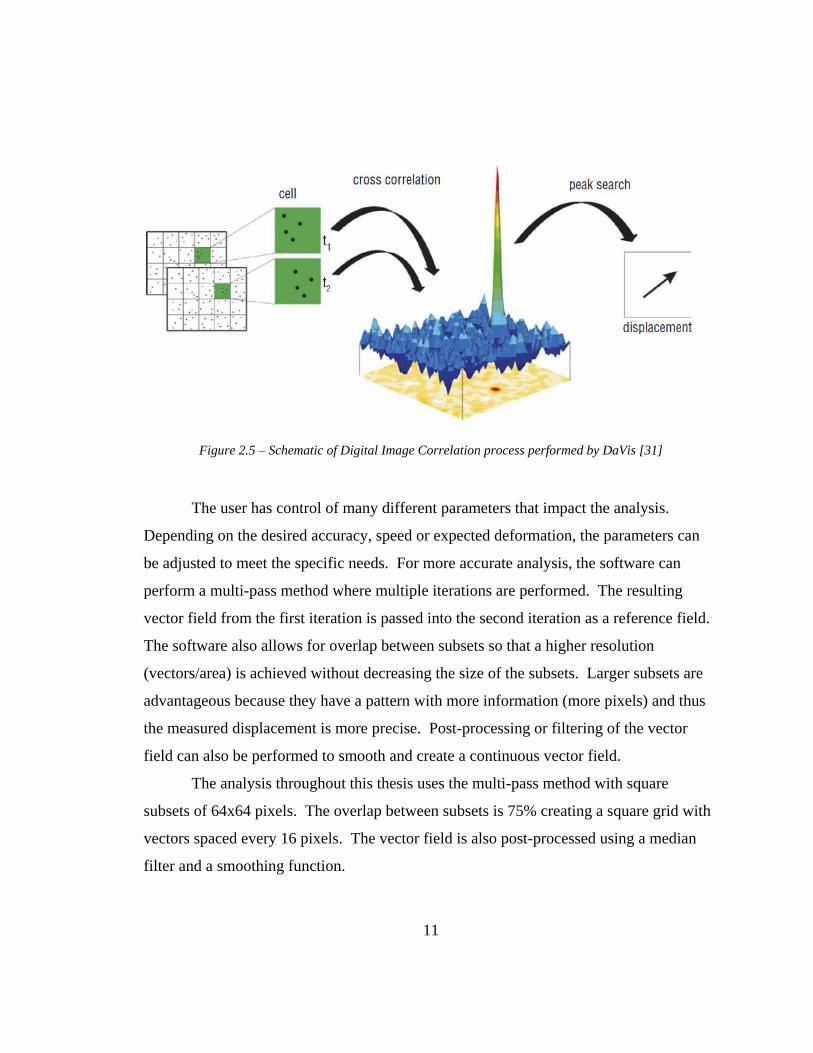
Figure 2.5 – Schematic of Digital Image Correlation process performed by DaVis [31]

The user has control of many different parameters that impact the analysis.

Depending on the desired accuracy, speed or expected deformation, the parameters can

be adjusted to meet the specific needs. For more accurate analysis, the software can

perform a multi-pass method where multiple iterations are performed. The resulting

vector field from the first iteration is passed into the second iteration as a reference field.

The software also allows for overlap between subsets so that a higher resolution

(vectors/area) is achieved without decreasing the size of the subsets. Larger subsets are

advantageous because they have a pattern with more information (more pixels) and thus

the measured displacement is more precise. Post-processing or filtering of the vector

field can also be performed to smooth and create a continuous vector field.

The analysis throughout this thesis uses the multi-pass method with square

subsets of 64x64 pixels. The overlap between subsets is 75% creating a square grid with

vectors spaced every 16 pixels. The vector field is also post-processed using a median

filter and a smoothing function.

12

Chapter 3: Fatigue Crack Growth – Theoretical

Framework

3.1 Fatigue Crack Growth at the Large-size Limit

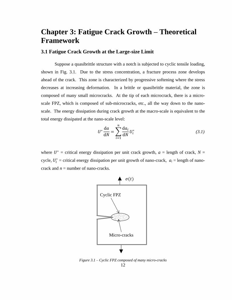
Suppose a quasibrittle structure with a notch is subjected to cyclic tensile loading,

shown in Fig. 3.1. Due to the stress concentration, a fracture process zone develops

ahead of the crack. This zone is characterized by progressive softening where the stress

decreases at increasing deformation. In a brittle or quasibrittle material, the zone is

composed of many small microcracks. At the tip of each microcrack, there is a micro-

scale FPZ, which is composed of sub-microcracks, etc., all the way down to the nano-

scale. The energy dissipation during crack growth at the macro-scale is equivalent to the

total energy dissipated at the nano-scale level:

∑

(3.1)

where = critical energy dissipation per unit crack growth, a = length of crack, N =

cycle, = critical energy dissipation per unit growth of nano-crack, ai = length of nano-

crack and n = number of nano-cracks.

Figure 3.1 – Cyclic FPZ composed of many micro-cracks

Cyclic FPZ

Micro-cracks

𝜎(𝑡)

13

Le and Bazant explained that a crack in a nano-scale element does not advance

smoothly but rather advances in discrete jumps, which corresponds to the jump over the

activation energy barriers of the nano-particle connectors [42]. It was shown that the

nano-crack growth rate under constant stress is related to the frequency of crack jumps in

a nano-element:

⁄ (3.2)

where Q0 = the dominant activation energy barrier on the free energy potential surface, k

= the Boltzmann constant, T = absolute temperature, Ka = the stress intensity factor of the

nano-element, ( ) ⁄ , = the spacing of nano-particles, = the

perimeter of the radial crack front, h = 6.626 x 10-34

and E1 = the Young’s modulus of

the nano-element. If the stress is cyclic, the equation can be written as:

⁄ (3.3)

where ΔK = amplitude of the stress intensity factor. This equation resembles the Paris-

Erdogan law with an exponent of 2. Nevertheless, the classical Paris-Erdogan law for

quasibrittle materials usually has an exponent, m, greater than 10. Substituting Eqn. 3.3

into Eqn. 3.1:

∑

(3.4)

Since there are numerous nano-cracks in the FPZ, the summation can be

expressed as:

∑

(3.5)

where = the average stress intensity factor of the nano-cracks. Within the LEFM

framework, the stress intensity factor amplitude of a nano-crack is proportional to the

stress intensity factor amplitude of the macro-crack.

14

Therefore, Eqn. 3.4 yields:

( ) (3.6)

The number of nano-cracks, n, can be expressed as a function of the stress

intensity factor, Young’s Modulus (E) and critical energy dissipation. Using dimensional

analysis, n depends on the dimensionless quantity ⁄ . Further assuming self-

similarity (i.e., power law):

(

) (

)

(3.7)

Substituting Eqn. 3.7 into Equation 3.6 yields:

( ) (3.8)

Assuming A/Em can be rewritten as a new constant, C, and p = 4m:

( ) ⁄ (3.9)

Eqn. 3.9 represents a fatigue crack growth law for the large-size limit. It agrees

well with the original Paris-Erdogan law, which has been applied to quasibrittle

structures [43, 44, 45]. The power law relation stems from the hypothesis of self-

similarity of function f, presented in Eqn. 3.7. This hypothesis holds well for the

medium stress amplitudes but deviates for very small or very large amplitudes. Le and

Bazant [42] explain that at small amplitudes (ΔK → 0), the distinction between static and

cyclic FPZs may become blurred causing the deviation from self-similarity. For large

amplitudes (ΔK → KIc), the failure may be dynamic because the stress amplitude

approaches the fracture toughness. Many experiments have shown the power-law

deviation at both limits [1, 25, 46].

15

3.2 Scaling of Fatigue Crack Growth Law

The forgoing analysis is limited to structures that are much larger than the FPZ

size (i.e., the large-size limit). In order to apply Eqn. 3.9 for smaller sizes, a scaling

relationship will be introduced for the critical energy dissipation, U*. It is assumed that

this relationship takes a form similar to the scaling of fracture energy, Gf, which is

derived from the size effect law on nominal monotonic strength:

√ ⁄ (3.10)

where ft’ = tensile strength of the material, B = dimensionless constant and D0m = the

transitional size for monotonic loading. The nominal strength is reached when the stress

intensity factor is equal to the critical stress intensity factor KIc, which can be written in

the following form:

√ ( ) (3.11)

Substituting the relationship between fracture energy and fracture toughness,

( ) into Eqn. 3.11 and solving for the nominal strength yields:

( ) (3.12)

where ( ) ( ) . Equation 3.12 is equal to Eqn. 3.10 squared:

( )

( )

( ⁄ ) (3.13)

Simplifying Eqn. 3.13, the size effect on fracture energy can be written as:

[

] (3.14)

where ( )

( ) ⁄ , which is the fracture energy for an infinitely sized

specimen [26].

16

The first hypothesis is that the size effect on the critical energy dissipation, U*,

takes the form of Eqn. 3.13 and can be expressed as:

[

] (3.15)

where is the critical energy dissipation per unit crack growth for a infinitely sized

specimen and D0c = the transitional size under cyclic loading. The equation holds for

infinitely sized specimens, ( ) and as D → 0, the energy dissipation goes to zero.

Combining Eqn. 3.9 into Eqn. 3.7, the final equation for the size-dependent Paris-

Erdogan law is

[ √

]

(3.16)

Since is a very difficult parameter to determine, it can be combined into the constant

C, which is fit to experimental data. This equation is very similar to the equation

proposed by Bažant and Xu [43], which was scaled by normalizing the amplitude of the

stress intensity factor by the size-dependent critical stress intensity factor, KIc. Bažant

and Xu found that the optimum fit was achieved when the transitional size used for cyclic

loading, D0c, was much larger than the transitional size computed during monotonic

loading, D0m.

The second hypothesis is that the transitional size for both monotonic and cyclic

loading can be expressed as:

( ) (3.17)

where γ = a non-dimensional constant and lpm and lpc = the length of the fracture process

zone under monotonic and cyclic loading, respectively. Eqn. 3.17 states that the change

in D0i from monotonic loading to cyclic loading is purely due to the change in FPZ size

from monotonic to cyclic loading. Experimental verification is essential to test the

hypotheses.

17

Chapter 4: Monotonic Size Effect Test

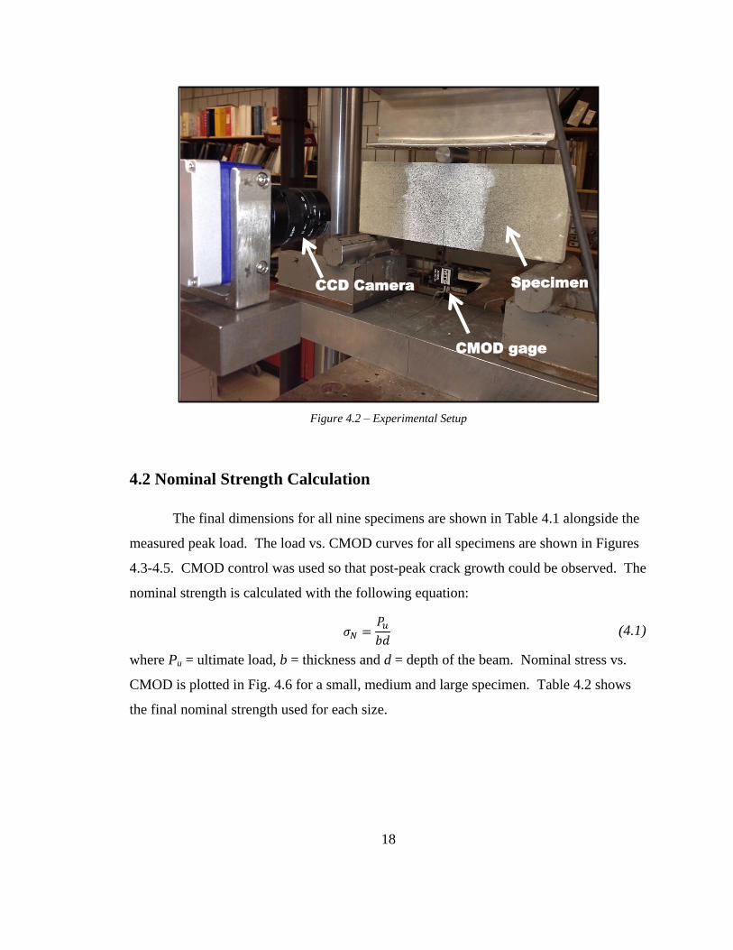
4.1 Experimental Setup

Prior to conducting fatigue tests, monotonic three-point tests were performed to

determine the size effect on nominal strength and investigate the fracture process zone

size. A total of nine specimens, three of each size, were tested using a closed-loop, servo

hydraulic 1 MN load frame (MTS Systems, Eden Prairie, MN). The nominal dimensions

of the specimens are shown in Fig. 4.1. The setup for monotonic loading is fairly simple

and is shown in Fig 4.2. The specimen is centered between two supports and the load is

applied at the center of the beam. A charge-coupled device (CCD) camera is attached to

a fixed frame and takes pictures for digital image correlation. A clip gage measures the

crack mouth opening displacement (CMOD).

To increase the accuracy of the digital image correlation process, the surface of

the specimen is painted with black and white paint. The surface is first coated with white

paint and then sprayed lightly with black spray paint. The result is a surface that has

unique patterns of speckles.

Figure 4.1 – Specimen Geometry for three-point bending tests

d

S = 2.5d

b = 20mm

a0 = 0.2d

Small: d = 25.4mm

Medium: d = 50.8mm

Large: d = 101.6mm

18

Figure 4.2 – Experimental Setup

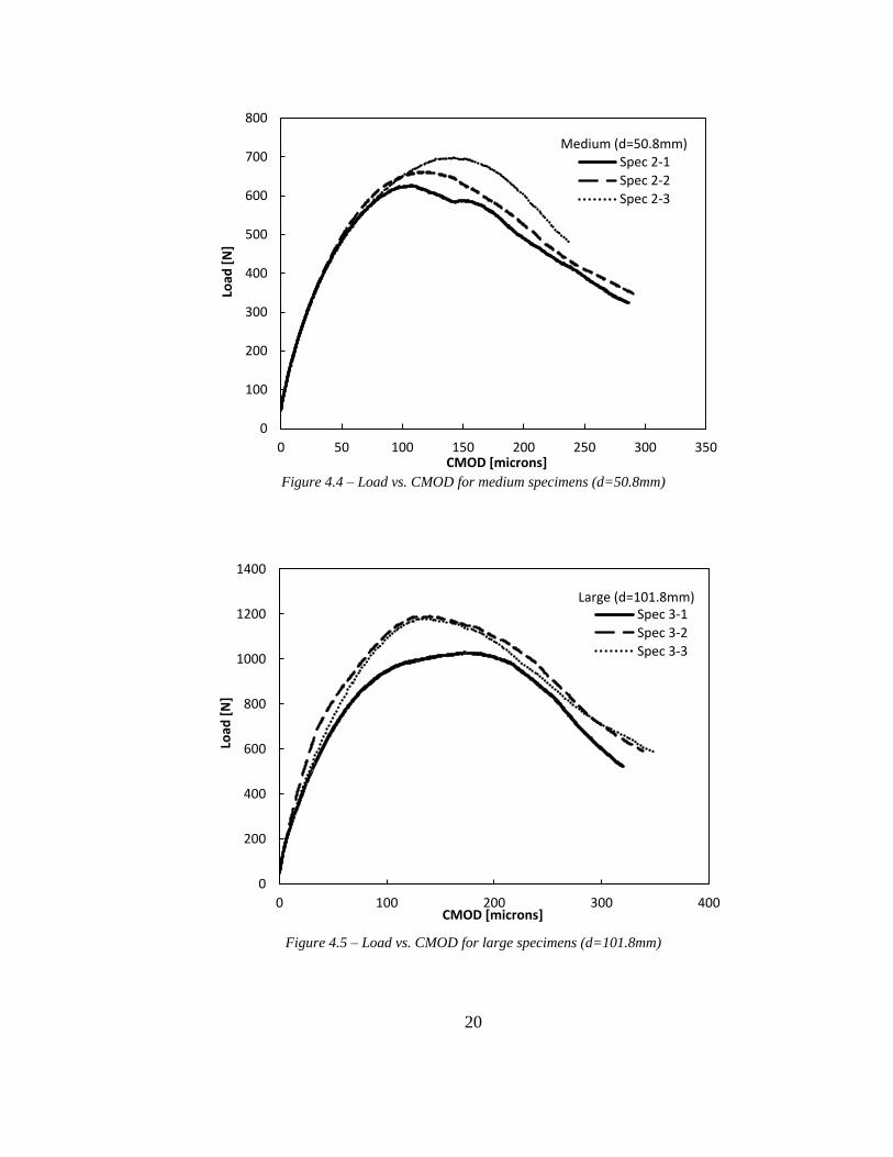
4.2 Nominal Strength Calculation

The final dimensions for all nine specimens are shown in Table 4.1 alongside the

measured peak load. The load vs. CMOD curves for all specimens are shown in Figures

4.3-4.5. CMOD control was used so that post-peak crack growth could be observed. The

nominal strength is calculated with the following equation:

(4.1)

where Pu = ultimate load, b = thickness and d = depth of the beam. Nominal stress vs.

CMOD is plotted in Fig. 4.6 for a small, medium and large specimen. Table 4.2 shows

the final nominal strength used for each size.

CCD Camera

CMOD gage

Specimen

19

Table 4.1: Specimen properties for monotonic loading

Specimen S[mm] a0

[mm] b [mm] d [mm] Pu [N]

σn [MPa]

Sma

ll Spec. 1-1 63.50 5.38 20.01 25.40 381.8 0.751

Spec. 1-2 63.50 5.51 19.99 25.38 404.5 0.797

Spec. 1-3 63.50 5.21 20.02 25.45 464.9 0.912

Med

ium

Spec. 2-1 127.00 11.20 20.14 50.83 626.2 0.612

Spec. 2-2 127.00 10.80 20.08 50.58 662.0 0.652

Spec. 2-3 127.00 10.49 20.08 50.66 698.7 0.687

Larg

e Spec. 3-1 254.00 20.43 20.04 101.62 1029 0.505

Spec. 3-2 254.00 20.57 20.02 101.70 1190 0.584

Spec. 3-3 254.00 20.72 20.19 101.73 1178 0.573

Table 4.2: Average nominal strength

Figure 4.3 – Load vs. CMOD for small specimens (d=25.4mm)

0

50

100

150

200

250

300

350

400

450

500

0 50 100 150 200

Load

[N

]

CMOD [microns]

Spec 1-1

Spec 1-2

Spec 1-3

Small (d=25.4mm)

Size Average nominal strength

Small 0.820 MPa

Medium 0.650 MPa

Large 0.554 MPa

20

Figure 4.4 – Load vs. CMOD for medium specimens (d=50.8mm)

Figure 4.5 – Load vs. CMOD for large specimens (d=101.8mm)

0

100

200

300

400

500

600

700

800

0 50 100 150 200 250 300 350

Load

[N

]

CMOD [microns]

Spec 2-1

Spec 2-2

Spec 2-3

Medium (d=50.8mm)

0

200

400

600

800

1000

1200

1400

0 100 200 300 400

Load

[N

]

CMOD [microns]

Spec 3-1

Spec 3-2

Spec 3-3

Large (d=101.8mm)

21

Figure 4.6 – Nominal strength vs. CMOD for one specimen of each size

0.0

0.1

0.2

0.3

0.4

0.5

0.6

0.7

0.8

0.9

0 100 200 300 400

σn

[MP

a]

CMOD [microns]

Small (Spec 1-2)Medium (spec 2-2)Large (Spec 3-2)

22

4.3 Fracture Properties from Size Effect Method

The size effect of the ultimate nominal stress (σNu), shown in Table 4.2 and Fig.

4.6, can be characterized by Bažant’s size effect equation [25]:

√ ⁄ (4.2)

where = tensile strength of the material, D = size of specimen, B = dimensionless

constant and D0 = constant with dimension of length. This equation can be algebraically

rearranged to a linear equation in the following form:

(4.3)

where

,

,

√ ,

(4.4)

Fig. 4.7 shows the regression plot used to compute the constants A and C. D0 and

B are both functions of these constants, as shown in Eqn. 4.4, and are also related to

the classical fracture parameters by the following equations,

√ (4.5)

(4.6)

( )

(4.7)

where KIf = fracture toughness, cf = critical effective crack extension for a semi-infinite

crack in an infinite body, Gf = critical energy release rate, k0 = the dimensionless stress

intensity factor computed from LEFM.

23

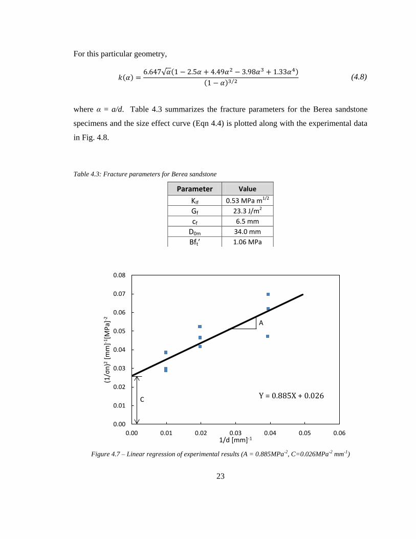
For this particular geometry,

( ) √ ( )

( ) ⁄ (4.8)

where α = a/d. Table 4.3 summarizes the fracture parameters for the Berea sandstone

specimens and the size effect curve (Eqn 4.4) is plotted along with the experimental data

in Fig. 4.8.

Table 4.3: Fracture parameters for Berea sandstone

Figure 4.7 – Linear regression of experimental results (A = 0.885MPa-2, C=0.026MPa-2 mm-1)

Y = 0.885X + 0.026

0.00

0.01

0.02

0.03

0.04

0.05

0.06

0.07

0.08

0.00 0.01 0.02 0.03 0.04 0.05 0.06

(1/σ

n)2

[m

m]-1

[MP

a]-2

1/d [mm]-1

C

A

Parameter Value

KIf 0.53 MPa m1/2

Gf 23.3 J/m2

cf 6.5 mm

D0m 34.0 mm

Bft’ 1.06 MPa

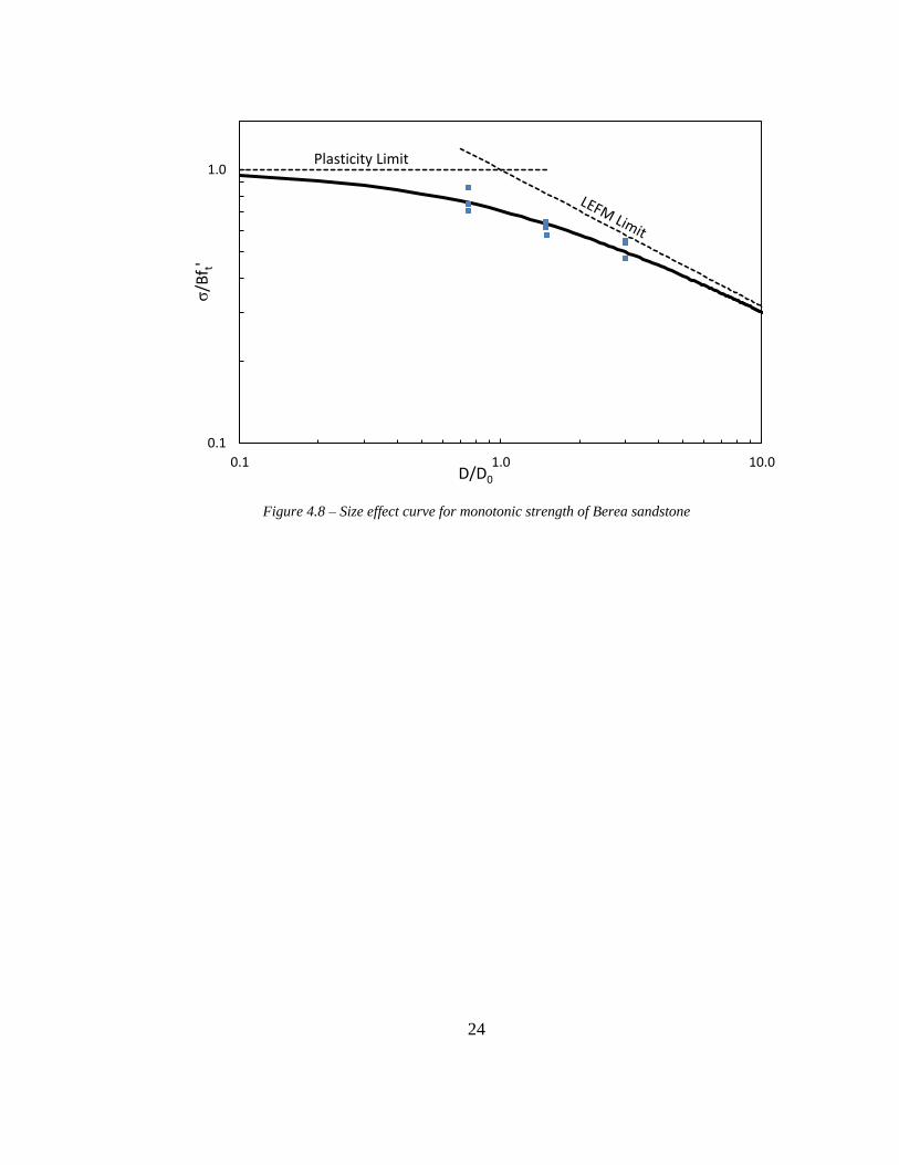
24

Figure 4.8 – Size effect curve for monotonic strength of Berea sandstone

0.1

1.0

0.1 1.0 10.0

σ/B

f t'

D/D0

Plasticity Limit

25

4.4 Fracture Process Zone Size

Analyzing the displacement fields from digital image correlation (DIC) provides a

way to estimate the size of the fracture process zone. This zone, in front of a crack tip, is

considered a material property and travels with a propagating crack. In a three-point

bending test, a stress concentration appears near the notch tip causing this non-linear

fracture process zone to develop.

Fig. 4.9 shows the horizontal displacement contours for an interval from 30-40%

peak load for a medium-sized specimen. The notch-tip is at point (0, 0) and the notch is

shown by a white box. The contours show that the material is moving to the right

(positive displacement) on the right side of the notch and to the left (negative

displacement) on the left side of the notch. The contours merge at the notch tip.

Figure 4.9 – Incremental horizontal displacement contours for a medium sized specimen from 30-40% peak

load

26

To better understand the behavior near the tip, it is helpful to look at the

displacements along a horizontal cross section. For instance, Fig. 4.10a shows the

horizontal displacement values along a horizontal line 0.3 mm above the notch tip. The

influence of the notch is shown by an increase in the gradient (∂ux/∂x). If a cross section

is taken farther away from the notch, the gradient decreases, as shown in Fig. 4.10b for a

horizontal line taken at y = 2.5 mm. The gradient will become zero at the neutral axis.

(a) (b)

Figure 4.10 –Horizontal displacement measurements from 30% to 40% peak load along horizontal lines

at (a) y = 0.3mm. (b) y = 2.5mm

-3.0

-2.0

-1.0

0.0

1.0

2.0

3.0

-15 -5 5 15

ux

(mic

ron

)

x (mm)

𝜕𝑢

𝜕𝑥 0 × 0

y = 0.3mm

-3.0

-2.0

-1.0

0.0

1.0

2.0

3.0

-15 -5 5 15

ux

(mic

ron

)

x (mm)

𝜕𝑢

𝜕𝑥 0 × 0

y = 2.5mm

27

As the load increases, a damage zone develops. Lin and Labuz [31] showed that

the tip of this zone is represented by the location where horizontal displacement contours

merge. Fig. 4.11 shows the incremental horizontal displacement contours from 60%-70%

peak load. The contours merge at a location y = 4 mm. The horizontal cross section

directly above the notch tip (y = 0.3 mm) displays an even larger gradient, shown in Fig.

4.12a. Moving farther from the notch tip causes the gradient to decrease as shown in

Figures 4.12b-d.

Figure 4.11 – Incremental horizontal displacement contours for a medium sized specimen

from 60-70% peak load

Tip

28

(a) (b)

(c) (d)

Figure 4.12 –Horizontal displacement measurements from 60% to 70% peak load along the line

(a) y = 0.3 mm. (b) y = 2.5 mm (c) y = 5.0 mm (d) y=9.0 mm

The fracture process zone is assumed to be fully developed once the specimen

reaches the peak load. Figure 4.13 shows the horizontal displacement contours for 90-

100% peak load. The tip of the damage zone is at approximately y = 9 mm and thus the

length of the fully-developed fracture process zone is 9 mm.

As the specimen continues into the post-peak regime, unstable crack propagation

begins. At peak load, the traction-free crack is assumed to form and as it propagates, the

load capacity of the specimen decreases. To estimate the length of this traction-free

-3.0

-2.0

-1.0

0.0

1.0

2.0

3.0

4.0

-15 -5 5 15

ux

(mic

ron

)

x (mm)

𝜕𝑢

𝜕𝑥 × 0

y=0.3 mm

-3.0

-2.0

-1.0

0.0

1.0

2.0

3.0

4.0

-15 -5 5 15

ux

(mic

ron

)

x (mm)

𝜕𝑢

𝜕𝑥 0 × 0

y=2.5 mm

-3.0

-2.0

-1.0

0.0

1.0

2.0

3.0

4.0

-15 -5 5 15ux

(mic

ron

)

x (mm)

𝜕𝑢

𝜕𝑥 0 × 0

y=5.0 mm

-3.0

-2.0

-1.0

0.0

1.0

2.0

3.0

4.0

-15 -5 5 15ux

(mic

ron

)

x (mm)

𝜕𝑢

𝜕𝑥 0 × 0

y=9.0 mm

29

surface, another measurement, called the critical opening displacement, ωc, must be

identified. Because it is impossible to pinpoint the tortuous crack path and measure

exactly at the crack face, the opening displacement will instead be measured a few

millimeters away. Fig. 4.13b shows the total displacement measurements from 70% pre-

peak to 100% peak along two vertical lines located at x = 1.7 mm and x = -1.6 mm. The

critical opening displacement, which represents the threshold for a traction free surface, is

the distance between the two lines at y = 0 mm. For this particular specimen ωc = 51 μm.

(a) (b)

Figure 4.13 – (a) Incremental horizontal displacement contours for a medium sized specimen from

90-100% peak load (b) Total horizontal displacement measurements along vertical lines at x = -1.6mm

(left line) and x = 1.7mm (right line)

-5

0

5

10

15

20

25

30

35

-40 -20 0 20 40

y (m

m)

ux (micron)

wc

Tip

30

(a) (b)

Figure 4.14 – (a) Incremental horizontal displacement contours for a medium sized specimen from 100%

peak -90% post-peak (b) Total horizontal displacement measurements along vertical lines at x = -1.6mm

(left line) and x = 1.7mm (right line)

Using the critical opening displacement, it is now possible to locate the tip of the

traction free surface post-peak. Fig. 4.14a shows the displacement contours from 100%

peak to 90% post-peak and the tip of the fracture process zone is at about y = 15 mm.

Fig. 4.14b shows that the traction free crack extends up to y = 8.5 mm, and thus the

process zone is about 6.5 mm in length. Fig. 4.15 summarizes the fracture process zone

farther into post-peak and includes the two other medium specimens that were tested.

The average FPZ size for the medium specimens was 7 mm.

-5

0

5

10

15

20

25

30

35

-60 -30 0 30 60

y (m

m)

ux (micron)

wc

a

lp

wc

a

lp

Tip

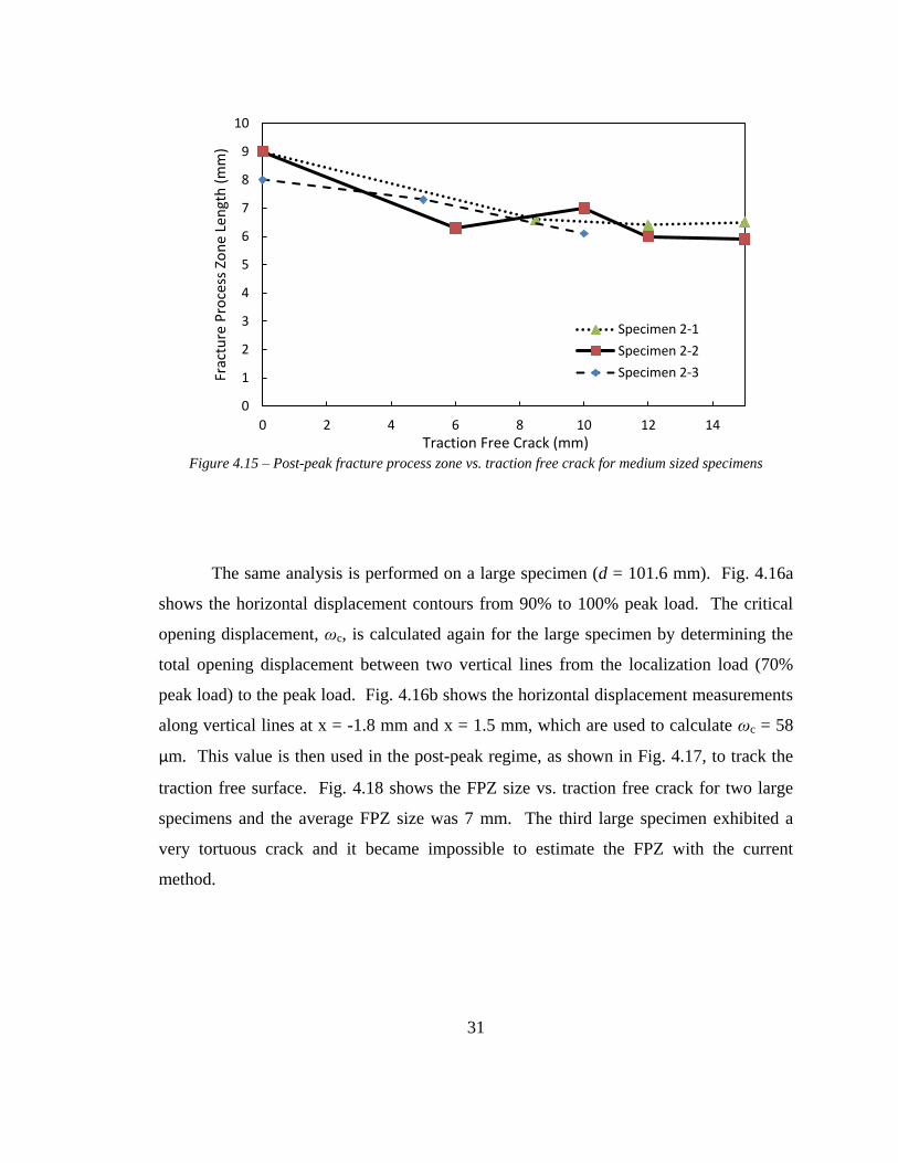
31

Figure 4.15 – Post-peak fracture process zone vs. traction free crack for medium sized specimens

The same analysis is performed on a large specimen (d = 101.6 mm). Fig. 4.16a

shows the horizontal displacement contours from 90% to 100% peak load. The critical

opening displacement, ωc, is calculated again for the large specimen by determining the

total opening displacement between two vertical lines from the localization load (70%

peak load) to the peak load. Fig. 4.16b shows the horizontal displacement measurements

along vertical lines at x = -1.8 mm and x = 1.5 mm, which are used to calculate ωc = 58

μm. This value is then used in the post-peak regime, as shown in Fig. 4.17, to track the

traction free surface. Fig. 4.18 shows the FPZ size vs. traction free crack for two large

specimens and the average FPZ size was 7 mm. The third large specimen exhibited a

very tortuous crack and it became impossible to estimate the FPZ with the current

method.

0

1

2

3

4

5

6

7

8

9

10

0 2 4 6 8 10 12 14

Frac

ture

Pro

cess

Zo

ne

Len

gth

(m

m)

Traction Free Crack (mm)

Specimen 2-1

Specimen 2-2

Specimen 2-3

32

(a) (b)

Figure 4.16 – (a) Incremental horizontal displacement contours for a large-size specimen from 95% pre

peak -100% post-peak (b) Total horizontal displacement measurements from 70% pre-peak to 100%peak

along vertical lines at x = -1.8mm (left line) and x = 1.5mm (right line)

The same procedure was used on the small-size specimens, shown in Fig. 4.19,

and it was found that the average FPZ size was 3.5 mm. This contradicts the assumption

that the FPZ size is independent of size, but there are other factors that may be at play.

Boundary effects may be causing a decrease in size because the small sized specimens

only have a ligament approximately 20mm in length. With some of the ligament in

compression, there may not be enough “room” for the FPZ to develop to its full size.

In conclusion, the length of the fully developed fracture process zone, lp, under

monotonic loading is 7 mm. The transitional size, D0m, is also known and thus the non-

dimensional parameter, γ, can be computed from Eqn. 3.17.

(4.8)

-5

0

5

10

15

20

25

30

35

-40 -20 0 20 40

y (m

m)

ux (micron)

wc

lp

Tip

33

. (a) (b)

Figure 4.17 – (a) Incremental horizontal displacement contours for a large-size specimen from 100% peak

-95% post-peak (b) Total horizontal displacement measurements from 70% pre-peak to 95%post-peak

along vertical lines at x = -1.8mm (left line) and x = 1.5mm (right line)

Figure 4.18 – Post-peak fracture process zone vs. traction free crack for large-sized specimens

-5

0

5

10

15

20

25

30

35

-60 -30 0 30 60

y (m

m)

ux (micron)

wc

a

lp

0

1

2

3

4

5

6

7

8

9

10

0 5 10 15

Frac

ture

Pro

cess

Zo

ne

Len

gth

(m

m)

Traction Free Crack (mm)

Specimen 3-2

Specimen 3-3

Tip

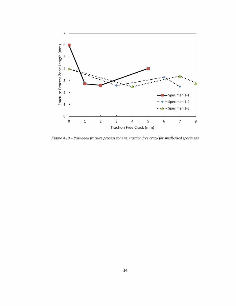
34

Figure 4.19 – Post-peak fracture process zone vs. traction free crack for small-sized specimens

0

1

2

3

4

5

6

7

0 1 2 3 4 5 6 7 8

Frac

ture

Pro

cess

Zo

ne

Len

gth

(m

m)

Traction Free Crack (mm)

Specimen 1-1

Specimen 1-2

Specimen 1-3

35

4.4 Displacement Gradient Method for Tracking Fracture Process Zone

In Sec. 4.3, a method was introduced to determine the length of the fracture

process zone that was developed by Lin & Labuz [31]. This method was based on

experiments that used both digital image correlation (DIC) and acoustic emission (AE) to

analyze the growth and propagation of the FPZ and it was found that the tip coincided

with the merging of horizontal displacement contours. In this section, another method

will be introduced that attempts to quantitatively characterize the behavior of the fracture

process zone by analyzing the displacement gradient.

The displacement gradient describes the change of displacement along a

continuous line segment:

𝜕𝑢

𝜕𝑥 (4.9)

where ux is the displacement in the x-direction. Fig. 4.11 shows the horizontal

displacement measurements along horizontal lines at different distances from the notch

tip. The stress concentration due to the notch results in an increase in the slope of the

line. The effect of the stress concentration is well pronounced when y = 0.3 mm (Fig.

4.12a) and becomes less pronounced as the distance away from the notch tip increases,

e.g. y = 9.0 mm (Fig. 4.12d). The slope of this line is the displacement gradient, g, and it

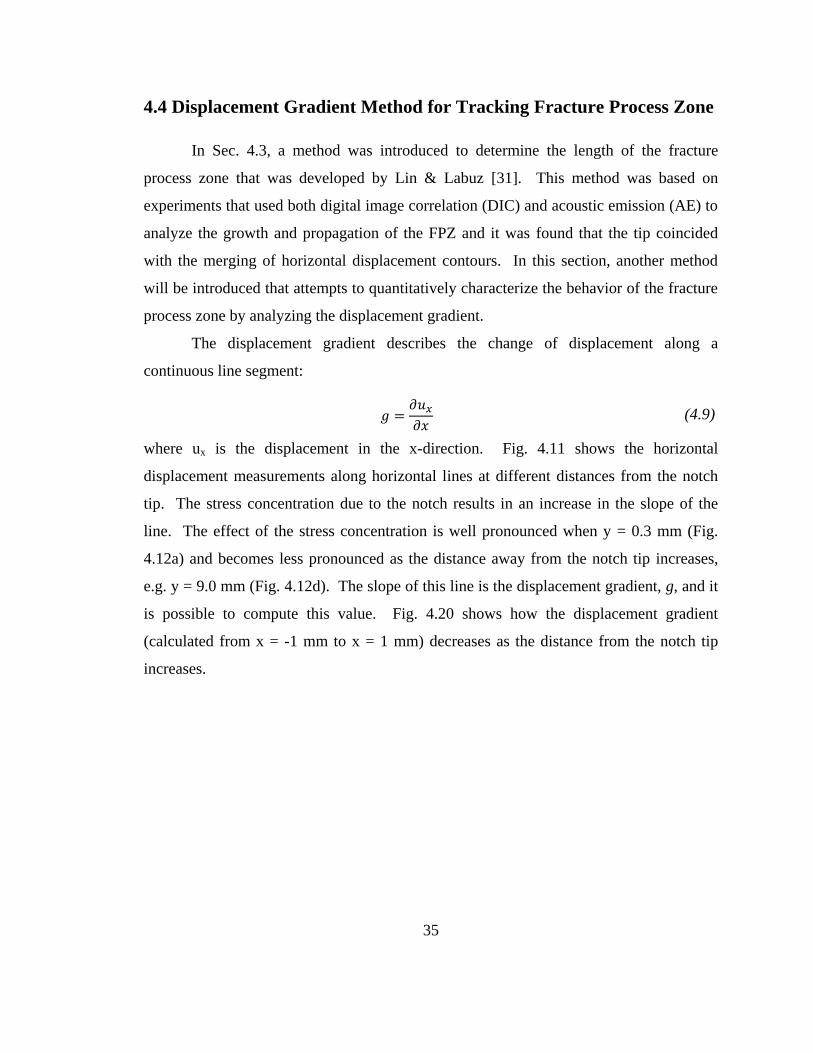
is possible to compute this value. Fig. 4.20 shows how the displacement gradient

(calculated from x = -1 mm to x = 1 mm) decreases as the distance from the notch tip

increases.

36

Figure 4.20 – Displacement gradient (from x=-1mm to x=1mm) vs. distance from the notch tip for a

medium sized specimen from 60% to 70% pre peak

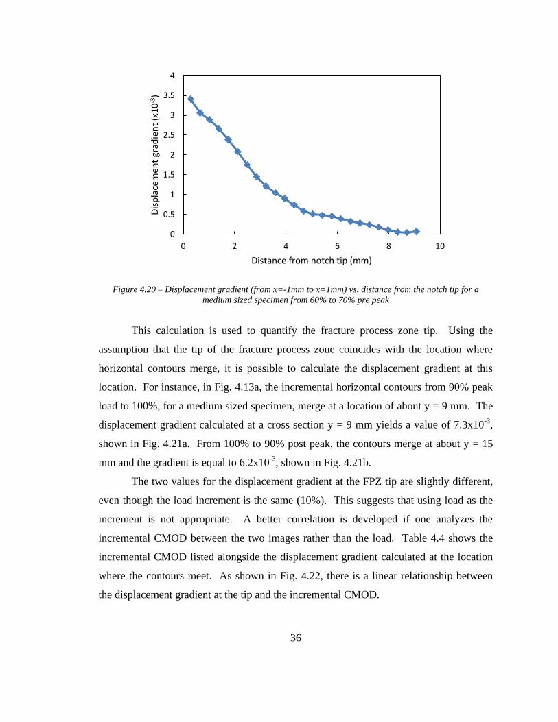
This calculation is used to quantify the fracture process zone tip. Using the

assumption that the tip of the fracture process zone coincides with the location where

horizontal contours merge, it is possible to calculate the displacement gradient at this

location. For instance, in Fig. 4.13a, the incremental horizontal contours from 90% peak

load to 100%, for a medium sized specimen, merge at a location of about y = 9 mm. The

displacement gradient calculated at a cross section y = 9 mm yields a value of 7.3x10-3

,

shown in Fig. 4.21a. From 100% to 90% post peak, the contours merge at about y = 15

mm and the gradient is equal to 6.2x10-3

, shown in Fig. 4.21b.

The two values for the displacement gradient at the FPZ tip are slightly different,

even though the load increment is the same (10%). This suggests that using load as the

increment is not appropriate. A better correlation is developed if one analyzes the

incremental CMOD between the two images rather than the load. Table 4.4 shows the

incremental CMOD listed alongside the displacement gradient calculated at the location

where the contours meet. As shown in Fig. 4.22, there is a linear relationship between

the displacement gradient at the tip and the incremental CMOD.

0

0.5

1

1.5

2

2.5

3

3.5

4

0 2 4 6 8 10

Dis

pla

cem

ent

grad

ien

t (x

10

-3)

Distance from notch tip (mm)

37

(a) (b)

Figure 4.21 – (a) Displacement gradient calculation at the tip (y=9mm) for 90% to 100% peak.

(b) Displacement gradient calculation at the tip (y=15mm) for 100% to 90% post-peak.

Table 4.4: Displacement gradient at tip of fracture process zone for a medium sized specimen

Load Increment FPZ

Location (mm)

CMOD Increment

(μm)

Displacement Gradient at

Tip (10-3)

70-80% pre-peak 3 12.6 2.6

80-90% pre-peak 5 17.4 3.0

90-100% pre-peak 9 46.5 7.3

100-90% post-peak 15 45.5 6.6

90-80% post-peak 19 30.9 4.6

80-70% post-peak 21 25 3.5

70-60% post-peak 24 35.3 4.8

Using this equation, one can calculate a limit where, if the displacement gradient

is above the limit, it is considered inside the FPZ and if it is below the limit, it is

considered outside the FPZ. For example, the incremental CMOD for a medium

specimen from 90% to 100% peak-load is 46.5 μm. The equation shown in Fig. 4.22

estimates the displacement gradient at the tip of the FPZ to be 6.8 x 10-3

. Figure 4.23a

shows the displacement gradient contour plot where the FPZ is gray and corresponds to

the region with displacement gradient is greater than 6.8 x 10-3

. Figure 4.23b shows the

FPZ during post-peak loading. This procedure may also be helpful to determine the

width of the process zone.

-10.0

-8.0

-6.0

-4.0

-2.0

0.0

2.0

4.0

6.0

8.0

10.0

-15 -5 5 15

ux

(mic

ron

)

x (mm)

𝜕𝑢

𝜕𝑥 × 0

-10.0

-8.0

-6.0

-4.0

-2.0

0.0

2.0

4.0

6.0

8.0

10.0

-15 -5 5 15

ux

(mic

ron

)

x (mm)

𝜕𝑢

𝜕𝑥 × 0

38

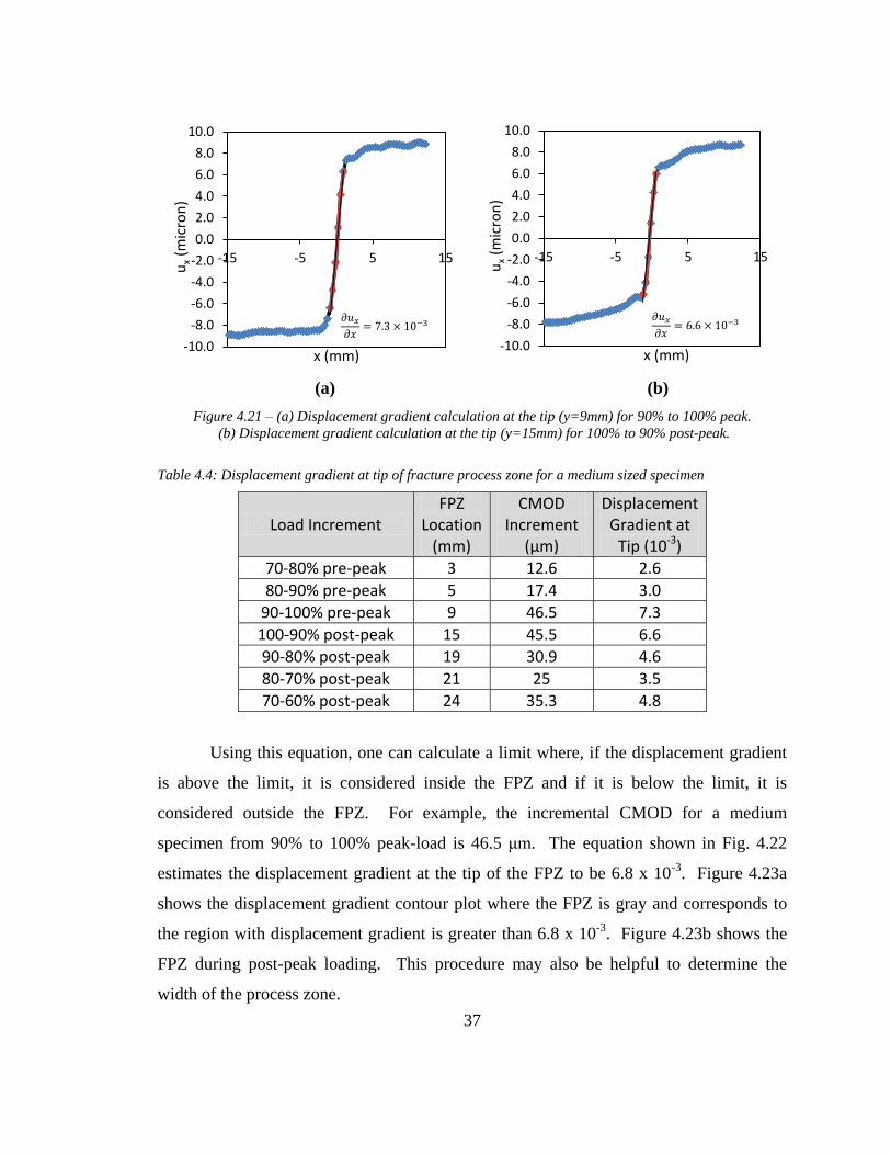
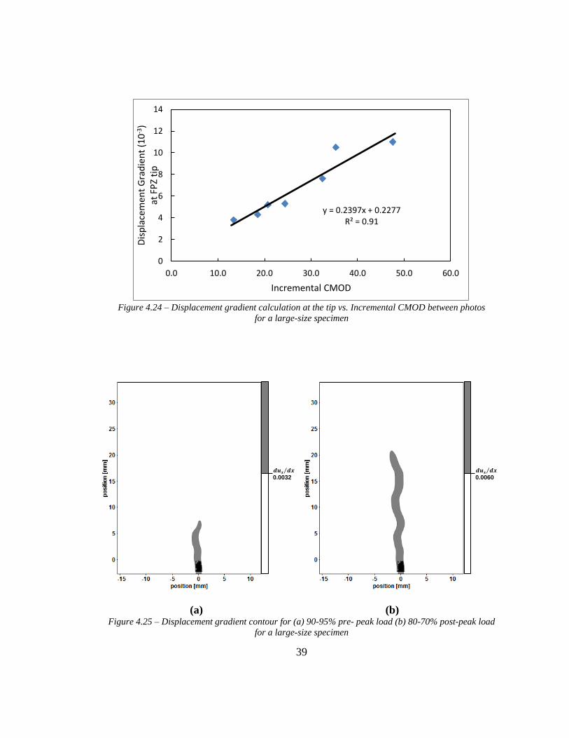
This approach was also implemented for a large specimen. Figure 4.24 shows the

linear relationship between the displacement gradient and the incremental CMOD, and

Figure 4.25 shows two displacement gradient plots that outline the fracture process zone.

Figure 4.22 – Displacement gradient calculation at the tip vs. Incremental CMOD between photos for a

medium-size specimen

(a) (b)

Figure 4.23 – Displacement gradient contour for (a) 90-100% peak load (b) 80-70% post-peak load

y = 0.1332x + 0.5642 R² = 0.9547

0

1

2

3

4

5

6

7

8

0 10 20 30 40 50

Dis

pla

cem

ent

Gra

die

nt

(10-3

)

at F

PZ

tip

Incremental CMOD (microns)

0.0068 𝒅𝒖𝒙 𝒅𝒙⁄

0.0039 𝒅𝒖𝒙 𝒅𝒙⁄

39

Figure 4.24 – Displacement gradient calculation at the tip vs. Incremental CMOD between photos

for a large-size specimen

(a) (b)

Figure 4.25 – Displacement gradient contour for (a) 90-95% pre- peak load (b) 80-70% post-peak load

for a large-size specimen

y = 0.2397x + 0.2277 R² = 0.91

0

2

4

6

8

10

12

14

0.0 10.0 20.0 30.0 40.0 50.0 60.0

Dis

pla

cem

ent

Gra

die

nt

(10

-3)

at

FP

Z ti

p

Incremental CMOD

0.0032 𝒅𝒖𝒙 𝒅𝒙⁄

0.0060 𝒅𝒖𝒙 𝒅𝒙⁄

40

Chapter 5: Size Effect Test on Fatigue Crack growth

5.1 Experimental Setup

Cyclic three-point bending experiments were performed to investigate size effect

on fatigue crack growth. The physical setup is identical to the monotonic test (Fig. 4.2),

the load, however, cycles between a maximum load, Pmax, and a minimum load, Pmin,

with a frequency of 1 Hz (Fig. 5.1). Crack mouth opening displacement (CMOD) is

recorded at the peak and valley of each cycle. The maximum load, Pmax, is set at

approximately 75% of the monotonic strength and Pmin is approximately 3%. One small

specimen, two medium specimens and one large specimen were prepared for cyclic

testing; dimensions are shown in Table 5.1.

Figure 5.1 – Load vs. time for cyclic three-point bending tests

Table 5.1: Specimen properties for cyclic loading

Specimen S [mm] a0 [mm] b [mm] d [mm] Pmax [N] Pmin [N]

Small Spec 1-4 63.50 5.37 19.99 25.47 310 15

Medium Spec 2-4 127.00 10.70 20.05 50.79 495 26

Medium Spec 2-5 127.00 11.45 20.04 50.89 480 28

Large Spec 3-4 254.00 20.05 20.16 100.55 930 33

Pmax

P

Pmin

t

. . .

P

a0

S

d

b = thickness

41

5.2 Compliance Calibration Method

To track crack growth through time, the compliance calibration method is used.

The displacement divided by the load is called the compliance and it is uniquely related

to geometry and crack length. Several investigators have used the compliance method to

determine crack length [47].

For this research, the compliance curve relates the CMOD compliance to an

effective crack ratio, α. This relationship was developed by modeling beams of different

notch lengths and computing the compliance using a finite element software, Abaqus ®.

The CMOD gauge does not measure the exact opening displacement of the notch, but

instead measures the displacement between two points where the CMOD clips are glued,

as shown in Fig. 5.2. Consideration was also taken to account for the thickness of the

CMOD clips. Fig 5.3 shows the final CMOD vs. effective crack length curves for the

three sizes with a Young’s modulus, E = 12 GPa.

Figure 5.2 – (Left) Zoomed-in view of CMOD gage, (Right) Numerical analysis performed with Abaqus

Gage

Length

1/2 Gage

Length

42

Figure 5.3 – CMOD vs. effective crack ratio for Young’s modulus = 12GPa

The measured compliance during the first cycle of loading should equal the

calculated compliance (from Fig. 5.3) for an effective crack ratio of α = a0/d where a0 is

the initial notch length d is the beam depth.. Any difference between the measured

compliance and the calculated compliance is assumed to be due to an effective Young’s

modulus in bending. The Young’s modulus used within the model is calibrated so that

the calculated compliance is equal to the measured compliance from the experiment.

Table 5.2 shows the Young’s modulus that was used for each beam. Once calibrated, a

polynomial is then fit to compute the effective crack length for a given CMOD

compliance.

0.000

0.050

0.100

0.150

0.200

0.250

0.300

0.00 0.10 0.20 0.30 0.40 0.50 0.60

CM

OD

Co

mp

lian

ce (

mic

ron

/N)

Effective crack ratio (a/d)

Small Beam (d=25.4mm)

Medium Beam (d=50.8mm)

Large Beam (d=101.8mm)

43

Table 5.2: Young’s modulus used to calibrate the CMOD compliance vs. effective crack curve for the first

cycle of loading

5.3 Paris-Erdogan Law Calculated from Compliance Method

Crack mouth opening displacement (CMOD) measurements were recorded at the

maximum (peak) and minimum (valley) load during each cycle. Figure 5.4 shows load

vs. CMOD measurements at different cycles. It is observed that the compliance increases

through time, which is a result of crack growth. Ultimately, the compliance begins to

increase at a faster rate and the specimen fails (Fig. 5.5). Using these measurements, the

compliance is computed:

(5.1)

where ΔP = the change in load and ΔCMOD = the change in crack mouth opening from

the minimum load to the maximum load. The effective crack length is then determined

using the calibrated curves from Fig. 5.3. Figure 5.6 shows the effective crack evolution

vs cycles for all four specimens.

Specimen α0

Cycle 1 CMOD

Compliance

[micron/N]

Young’s Modulus

[GPa]

Small – Specimen 1-4 0.21 0.063 6.25

Medium – Specimen 2-4 0.21 0.056 5.15

Medium – Specimen 2-5 0.23 0.053 5.80

Large – Specimen 2-4 0.20 0.044 5.35

44

Figure 5.4 – Load vs CMOD for different cycles

Figure 5.5 – Peak and valley CMOD measurements vs number of cycles

0

50

100

150

200

250

300

350

400

450

0.0 10.0 20.0 30.0 40.0 50.0 60.0 70.0

Load

(N

)

CMOD (microns)

0

10

20

30

40

50

60

70

80

90

100

0 1000 2000 3000 4000 5000 6000

CM

OD

(m

icro

ns)

Cycles

Failure

45

Figure 5.6 – Effective crack evolution

The Paris-Erdogan law can be constructed for each specimen by computing the

crack growth rate (da/dN) using a forward difference equation:

( ) ( )

(5.2)

where a(N1) is the effective crack length at cycle number N1 and a(N2) is the effective

crack length at cycle number N2. The change in stress intensity factor (ΔK) is computed

using

( )

√ ( ) (5.3)

where Pmax and Pmin are the maximum and minimum applied loads, b = thickness, d =

depth and k(α) is the dimensionless stress intensity factor, given in Eqn. 4.8. The value

used for alpha (α) is the average of a(N1) and a(N2) divided by the depth, d.

0.00

0.05

0.10

0.15

0.20

0.25

0.30

0.35

0.40

0.45

0.50

10 100 1000 10000 100000

Effe

ctiv

e C

rack

Len

gth

Rat

io (

a e/d

)

Cycles

Small Spec 1-4

Medium Spec 2-5

Medium Spec 2-4

Large Spec 3-4

46

Figure 5.7 shows da/dN vs ΔK in a log-log scale for medium specimen 2-5. Note

that the classical Paris-Erdogan law will not explain the entire behavior of the specimen.

Instead, there appears to be four unique stages of crack growth. At the beginning of the

test, the specimen exhibits crack growth that decreases in speed, shown by stage I. This

phenomenon has been observed previously and is defined as small flaw growth [1, 48-

50]. The rate then reaches a somewhat constant value during cycles 3,000 to 8,000,

shown by stage II. During stage III, The specimen exhibits an increasing growth rate that

can be explained by the Paris-Erdogan law. The last stage is associated with fast crack

growth. Although stages I and II were present for all four specimens, this portion of each

experiment was removed so the focus was on the region that can be explained by the

Paris-Erdogan Law. For specimen 2-5, which is shown in Fig. 5.7 and Fig. 5.8, the

analysis is performed from cycle 8,000 to failure. Table 5.3 lists the first cycle that is

included in the analysis of the Paris-Erdogan law for the other three fatigue tests.

Figure 5.7 – da/dN for medium specimen 2-5 plotted on log-log scale

0.000

0.001

0.010

0.250

da/

dN

ΔK (MPa-m1/2)

Stage I

Stage II

Stage III

Stage IV

0.300 0.400 0.500

47

Figure 5.8 – Effective crack length ratio for specimen 2-5 showing

the four apparent stages of crack growth

Table 5.3: Cycles analyzed for Paris-Erdogan law

Specimen First cycle analyzed for

Paris-Erdogan Law

Total Cycles To

Failure

Small 1-4 2,000 5,827

Medium 2-4 10,000 13,911

Medium 2-5 8,000 10,701

Large 3-5 13,000 21,276

The Paris-Erdogan law for all four specimens is shown in Fig. 5.9. The interval

(N2 – N1) used to calculate the crack growth rate (Eqn. 5.2) varies for each specimen in an

attempt to capture approximately 20-40 points per specimen. Figure 5.10 displays the

best-fit lines using a fixed slope for all three sizes and combining the two medium sized

specimens.

0.20

0.25

0.30

0.35

0.40

0.45

0 2000 4000 6000 8000 10000 12000

Effe

ctiv

e C

rack

Len

gth

Rat

io (

a e/d

)

Cycles

I II III IV

48

Figure 5.9 – Paris-Erdogan law for all four specimens plotted individually

Figure 5.10 – Paris-Erdogan law for all three sizes with a fixed slope, m = 17.6

5E-05

0.0005

0.005

0.250

da/

dN

(m

m/c

ycle

)

ΔK (MPa-m1/2)

Spec 1-4Spec 2-4Spec 2-5Spec 3-4

0.300 0.400 0.500

m= 19.0 logC= 6.0 m= 14.8 logC= 2.8 m= 19.0 logC= 4.5 m= 21.7 logC= 3.9

5E-05

0.0005

0.005

0.250

da/

dN

(m

m/c

ycle

)

ΔK (MPa-m1/2)

Small (d=25.4mm)Medium (d=50.8mm)Large (d=101.6mm)

m = 17.6

log C = 5.28

log C = 3.91 log C = 2.61

0.300 0.400 0.500 0.550

49

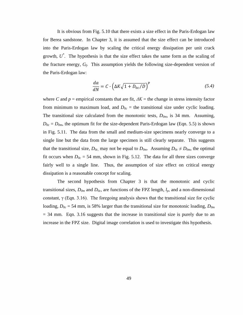
It is obvious from Fig. 5.10 that there exists a size effect in the Paris-Erdogan law

for Berea sandstone. In Chapter 3, it is assumed that the size effect can be introduced

into the Paris-Erdogan law by scaling the critical energy dissipation per unit crack

growth, U*. The hypothesis is that the size effect takes the same form as the scaling of

the fracture energy, Gf. This assumption yields the following size-dependent version of

the Paris-Erdogan law:

( √ ⁄ )

(5.4)

where C and p = empirical constants that are fit, ΔK = the change in stress intensity factor

from minimum to maximum load, and D0c = the transitional size under cyclic loading.

The transitional size calculated from the monotonic tests, D0m, is 34 mm. Assuming,

D0c = D0m, the optimum fit for the size-dependent Paris-Erdogan law (Eqn. 5.5) is shown

in Fig. 5.11. The data from the small and medium-size specimens nearly converge to a

single line but the data from the large specimen is still clearly separate. This suggests

that the transitional size, D0c, may not be equal to D0m. Assuming D0c ≠ D0m, the optimal

fit occurs when D0c = 54 mm, shown in Fig. 5.12. The data for all three sizes converge

fairly well to a single line. Thus, the assumption of size effect on critical energy

dissipation is a reasonable concept for scaling.

The second hypothesis from Chapter 3 is that the monotonic and cyclic

transitional sizes, D0m and D0c, are functions of the FPZ length, lp, and a non-dimensional

constant, γ (Eqn. 3.16). The foregoing analysis shows that the transitional size for cyclic

loading, D0c = 54 mm, is 58% larger than the transitional size for monotonic loading, D0m

= 34 mm. Eqn. 3.16 suggests that the increase in transitional size is purely due to an

increase in the FPZ size. Digital image correlation is used to investigate this hypothesis.

50

Figure 5.11 – Size-dependent Paris-Erdogan law using D0 = 34 mm

Figure 5.12 – Size-dependent Paris-Erdogan law using D0 = 54 mm

0.0001

0.001

0.40

da/

dN

ΔK·(1+D0/D)1/2 (MPa m1/2)

SmallMediumLarge

p = 17.6 log C = 2.37 logC = 2.23 log C= 1.66

D0 = 34 mm

0.500 0.600

0.0001

0.001

0.50

da/

dN

ΔK·(1+D0/D)1/2 (MPa m1/2)

SmallMediumLarge

p = 17.6 logC = 0.99

D0 = 54 mm

0.600 0.700

51

5.4 Fracture Process Zone Length – Cyclic Loading

From digital image correlation (DIC), the length of the fracture process zone

(FPZ) under monotonic loading was estimated to be 7mm (Chapter 4). The procedure is

replicated for the fatigue tests to investigate the growth and size of the FPZ during cyclic

loading.

In order to analyze the images in a consistent manner, it is important to consider

the digital images at a known load level. In the monotonic tests, photographs were taken

every two seconds, and it was possible to match the time of the photograph to the load

value that is recorded in the data file. This is much more difficult for a fatigue test that

can run for hours, with cycles between maximum and minimum load in 1 Hz. A system

was developed that is capable of triggering the CCD camera at a user-specified load

level. For all the cyclic tests, the camera was triggered at the maximum load and at the

minimum load once every 20 cycles. It is then possible to analyze the displacement

contour plots at different cycles to estimate the location of the FPZ.

As mentioned previously in Chapter 4, the tip of the FPZ coincides with the

location where the horizontal displacement contours merge. The region from the notch

tip to the FPZ tip is comprised of process zone and traction free length, although the

traction free surface exists only if the opening displacement between two vertical lines is

greater than the critical opening displacement, wc. The average critical opening

displacement from the monotonic experiments was approximately 40 μm for two lines

placed 3 mm apart.

Figure 5.13a shows the horizontal displacement contours from minimum to

maximum load for medium specimen 2-4 at cycle 6,000. The tip of the FPZ is estimated

to be at y = 5 mm. To determine if part of the damage zone is traction free surface, the

opening displacement between two vertical lines is analyzed. Figure 5.13b shows the

horizontal displacement measurements along lines at x = -1.6 mm and x = 1.6 mm. At

the notch tip (y = 0 mm), the total opening displacement between the two lines is 22 μm,

which is less than the critical opening displacement (wc = 40 μm). Thus, the entire region

is FPZ and the length is 5 mm.

52

. (a) (b)

Figure 5.13 – (a) horizontal displacement contours for medium specimen 2-4 – cycle 6,000

(b) Horizontal displacement measurements along vertical lines at x = -1.6 mm (left line) and x = 1.6 mm

(right line)

To reduce the amount of images recorded, photos are only taken once every 20

cycles and as a result, the final cycle may not be photographed. For this particular

specimen, the final cycle imaged is 13,900, which is 11 cycles before failure. Fig. 5.14a

shows the horizontal displacement contours for cycle 13,900 with the tip of the FPZ at y

= 10 mm. At the notch tip, the total opening displacement is 35 μm, which is still less

than the critical opening displacement (wc = 40 μm). Thus, the FPZ length is 10 mm. It

is impossible to determine if the FPZ grows any larger during the next 11 cycles or if

traction free surface begins to develop because no images were taken after cycle 13,900.

From the available data, it can be concluded that the cyclic FPZ length for this specimen

is at least 10 mm.

-5

0

5

10

15

20

25

30

-25 -13 0 13 25

y (m

m)

ux (micron)

lp

Tip

53

. (a) (b)

Figure 5.14 – (a) horizontal displacement contours for medium specimen 2-4 – cycle 13,900

(b) Horizontal displacement measurements along vertical lines at x = -1.6mm (left line) and x = 1.6mm

(right line)

The analysis is performed on a large specimen (specimen 3-4) and the horizontal

displacement contours for cycle 12,000 are shown in Fig. 5.15a. The tip of the process

zone is at approximately y = 8 mm and the opening displacement at the notch is 30μm,

meaning there is no traction free surface. For the medium specimen, there was no

traction free surface created until the very end. The large specimen, on the other hand,

displayed traction free surface growth around cycle 20,000, which is about 1,500 cycles

before failure.

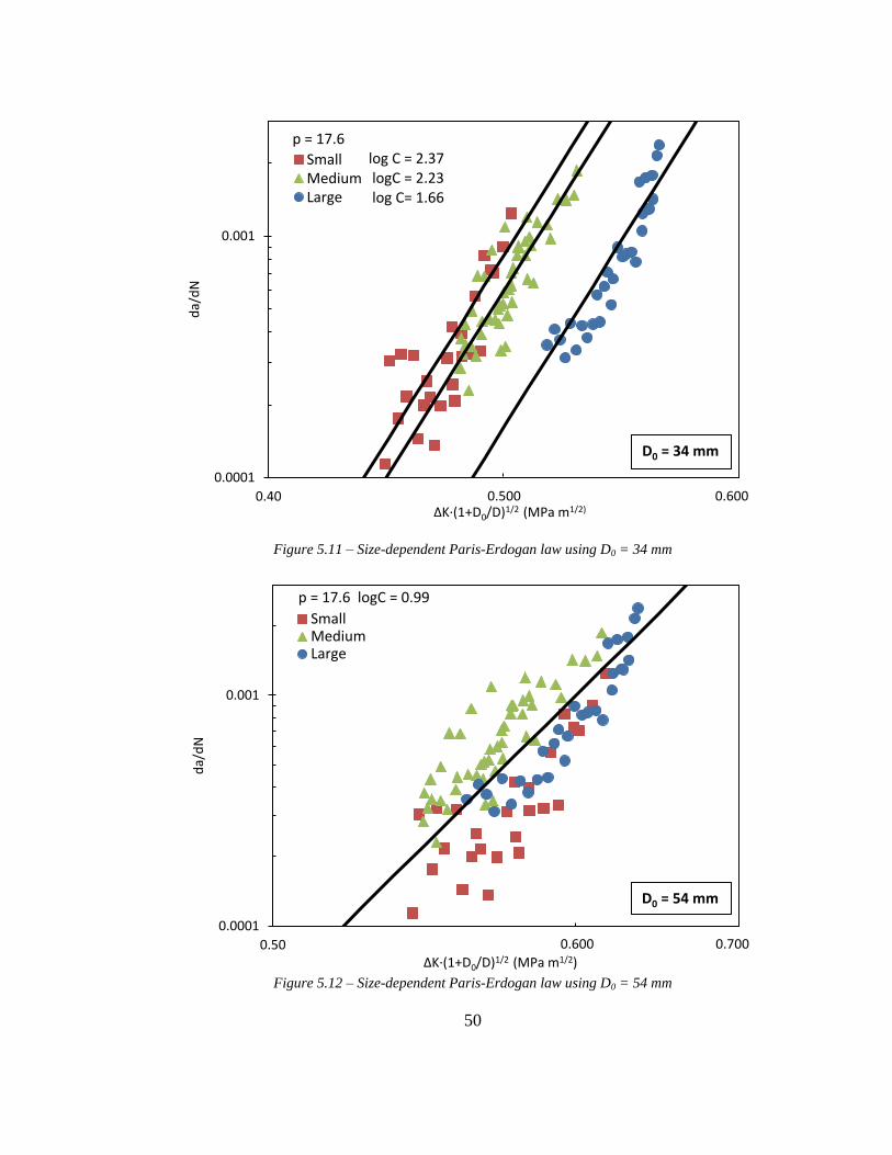
Fig. 5.16a shows the displacement contours for cycle 20,500, where the tip of the

FPZ is at 13 mm. Fig. 5.16b shows that the opening displacement between two vertical

lines at x = -1.4 mm and x = 1.8 mm exceeds the critical opening displacement and thus

some of this region is considered traction free. The opening displacement is 43 μm at the

notch tip and is 40 μm at y = 1.2 mm, meaning the traction free surface is 1.2 mm and the

FPZ length is 11.8 mm.

-5

0

5

10

15

20

25

30

-25 -13 0 13 25

y (m

m)

ux (micron)

lp

Tip

54

. (a) (b)

Figure 5.15 – (a) horizontal displacement contours for large specimen 3-4 – cycle 12,000

(b) Horizontal displacement measurements along vertical lines at x = -1.4mm (left line) and x = 1.8mm

(right line)

. (a) (b)

Figure 5.16 – (a) horizontal displacement contours for large specimen 3-4 – cycle 20,500

(b) Horizontal displacement measurements along vertical lines at x = -1.4mm (left line) and x = 1.8mm

(right line)

-5

5

15

25

35

45

-20 -10 0 10 20 30

y (m

m)

Δu (micron)

lp

-5

5

15

25

35

45

-40 -20 0 20 40

y (m

m)

Δu (micron)

lp

a

wc

Tip

Tip

55

. (a) (b)

Figure 5.17 – (a) horizontal displacement contours for large specimen 3-4 – cycle 21,260

(b) Horizontal displacement measurements along vertical lines at x = -1.4mm (left line) and x = 1.8mm

(right line)

Fig. 5.17a shows the displacement contours for cycle 21,260, which is 16 cycles

before failure. The tip of the FPZ is at y = 17 mm. The location where the opening

displacement is less than the critical opening displacement is at y = 7.0 mm, thus the FPZ

length for the large specimen is 10 mm. The average length of the FPZ calculated after

growth of traction free surface was 11 mm.

The same procedure is performed for the small specimen and the length of the

process zone during fatigue is 5 μm. This substantial decrease in size, compared to the

medium and large sized specimens, is similar to what was found during monotonic

loading. This is most likely caused by boundary effects that restrict the region where the

FPZ can develop.

-5

5

15

25

35

45

-40 -20 0 20 40

y (m

m)

Δu (micron)

lp

a

wc

Tip

56

Table 5.4 summarizes the FPZ sizes for all four fatigue tests. Also shown is the

monotonic FPZ length for each size. All four specimens generate a larger FPZ during

cyclic loading and the average increase is 43%.

Three of the four specimens did not exhibit any traction free surface until after the

last image was taken, and thus the length of the FPZ cannot be considered “fully-

developed.” This could explain why there was less increase in the FPZ size for the small

and medium size specimens. Only the large specimen displayed traction free growth and

thus the length of the fully-developed FPZ during cyclic loading is 11 mm. This value

can be used to compute the non-dimensional parameter, γ, from Eqn. 3.17:

(5.5)

The value for γ computed from monotonic loading was also 4.9, which supports the

hypothesis that the increase in transitional size is due to the increase in the fracture

process zone.

Table 5.4: Fracture process zone lengths for all four specimens

Specimen Cyclic FPZ length

(mm)

Monotonic FPZ length

(mm)

Percent increase in FPZ

size during cyclic

loading

Small 1-4 5 3.5 43%

Medium 2-4 10 7.0 43%

Medium 2-5 9 7.0 29%

Large 3-5 11 7.0 57%

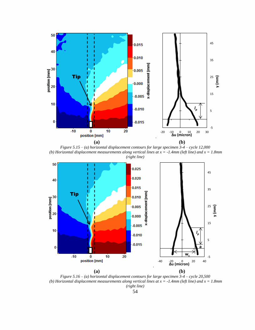
5.5 Paris-Erdogan Law calculated from DIC Method

Digital image correlation can also be implemented to look at the growth of the

damage zone through time. The difficulty in using the proposed method is that the

location where the fringes meet cannot be pinpointed more accurately than within a

millimeter. Fig. 5.18 shows the horizontal contours for cycle 2 with the tip at

approximately y = 1 mm. The final length of the process zone is 10 mm, and thus there

can only be 9 points to represent each time the FPZ length increases by approximately 1

mm, shown in Table 5.5.

57

For example, at cycle 100, the tip is estimated at y = 2 mm and at cycle 1,500, the tip is

estimated at y = 3 mm. In between cycles 100 and 1,499, growth can be observed but the

tip is still estimated at y = 2 mm. Cycle 1,500 represents the first time when the tip is

estimated at y = 3 mm.

Figure 5.18 – Horizontal displacement contours for cycle 2 for a medium specimen (2-4)

Table 5.5: Cycles where the FPZ tip increases by 1 mm for medium specimen 2-4

Cycle FPZ tip [mm]

2 1

100 2

1500 3

4000 4

6000 5

8500 6

10380 7

12880 8

13700 9

13900 10

Tip

58

An effective crack ratio that incorporates the damage zone can be represented by

the following equation:

(5.6)

where a0 = the initial crack length, Δae = the length of the damage zone determined from

DIC (FPZ + traction free surface) and d = depth of the beam. Figure 5.19 plots the

effective crack ratio from DIC (Eqn. 5.6) alongside the effective crack ratio estimated

from the compliance method. The results are fairly close throughout and this suggests

that the FPZ tip may be a good estimate for the length of the effective crack.

Figure 5.19 – Effective crack ratio vs. cycles computed using the compliance method and DIC method

The effective crack growth rate can be calculated using a forward difference

function (Eqn. 5.2) and the change in stress intensity factor can be calculated using the

alpha computed from DIC (Eqn. 5.6). Fig. 5.20 plots da/dN vs. ΔK from DIC method

alongside the data calculated from the compliance method for specimen 2-5. Despite the

limitations of the DIC method, the results lie close to the data from the compliance

method. The DIC method also observes a crack growth that decreases at the beginning of

the test that was shown in Fig. 5.7. As mentioned previously, the focus is to analyze the

0.00

0.05

0.10

0.15

0.20

0.25

0.30

0.35

0.40

0.45

0.50

10 100 1000 10000 100000

Effe

ctiv

e C

rack

Len

gth

Rat

io (

a e/d

)

Cycles

DIC Method

Compliance Method

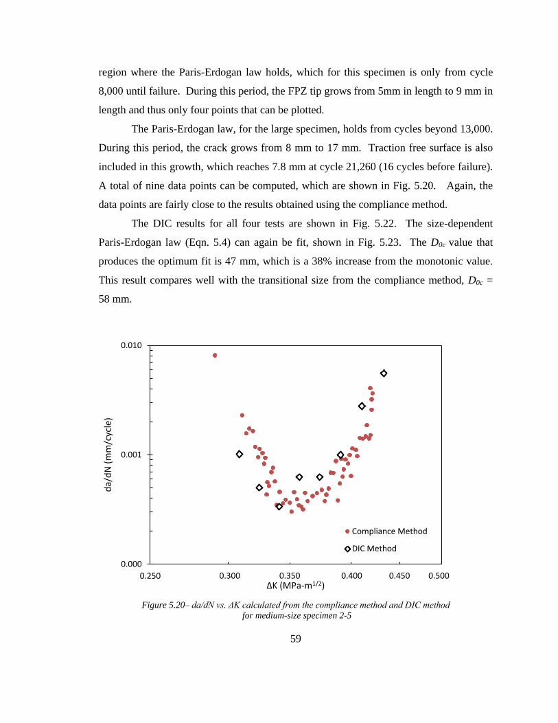
59

region where the Paris-Erdogan law holds, which for this specimen is only from cycle

8,000 until failure. During this period, the FPZ tip grows from 5mm in length to 9 mm in

length and thus only four points that can be plotted.

The Paris-Erdogan law, for the large specimen, holds from cycles beyond 13,000.

During this period, the crack grows from 8 mm to 17 mm. Traction free surface is also

included in this growth, which reaches 7.8 mm at cycle 21,260 (16 cycles before failure).

A total of nine data points can be computed, which are shown in Fig. 5.20. Again, the

data points are fairly close to the results obtained using the compliance method.

The DIC results for all four tests are shown in Fig. 5.22. The size-dependent

Paris-Erdogan law (Eqn. 5.4) can again be fit, shown in Fig. 5.23. The D0c value that

produces the optimum fit is 47 mm, which is a 38% increase from the monotonic value.

This result compares well with the transitional size from the compliance method, D0c =

58 mm.

Figure 5.20– da/dN vs. ΔK calculated from the compliance method and DIC method

for medium-size specimen 2-5

0.000

0.001

0.010

0.250

da/

dN

(m

m/c

ycle

)

ΔK (MPa-m1/2)

Compliance Method

DIC Method

0.300 0.350 0.400 0.450 0.500

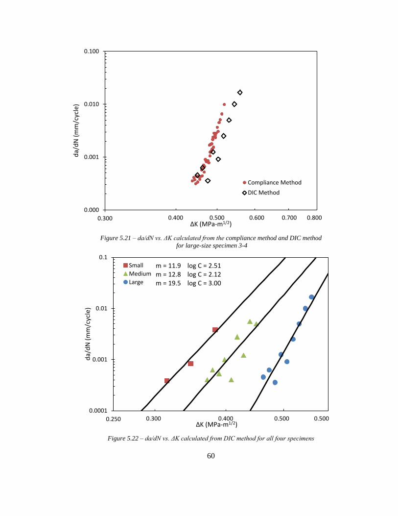
60

Figure 5.21 – da/dN vs. ΔK calculated from the compliance method and DIC method

for large-size specimen 3-4

Figure 5.22 – da/dN vs. ΔK calculated from DIC method for all four specimens

0.000

0.001

0.010

0.100

0.300

da/

dN

(m

m/c

ycle

)

ΔK (MPa-m1/2)

Compliance Method

DIC Method

0.400 0.500 0.600 0.700 0.800

0.0001

0.001

0.01

0.1

0.250

da/

dN

(m

m/c

ycle

)

ΔK (MPa-m1/2)

Small

Medium

Large

m = 11.9 log C = 2.51 m = 12.8 log C = 2.12 m = 19.5 log C = 3.00

0.300 0.400 0.500 0.500

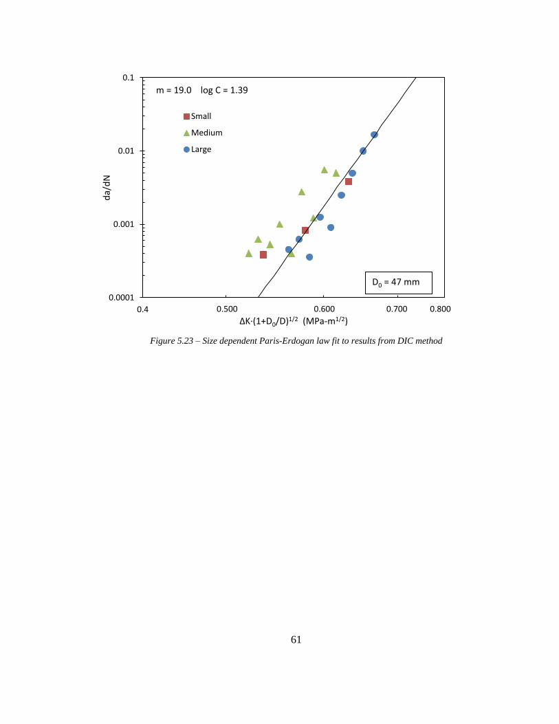
61

Figure 5.23 – Size dependent Paris-Erdogan law fit to results from DIC method

0.0001

0.001

0.01

0.1

0.4

da/

dN

ΔK·(1+D0/D)1/2 (MPa-m1/2)

Small

Medium

Large

m = 19.0 log C = 1.39

D0 = 47 mm

0.500 0.600 0.700 0.800

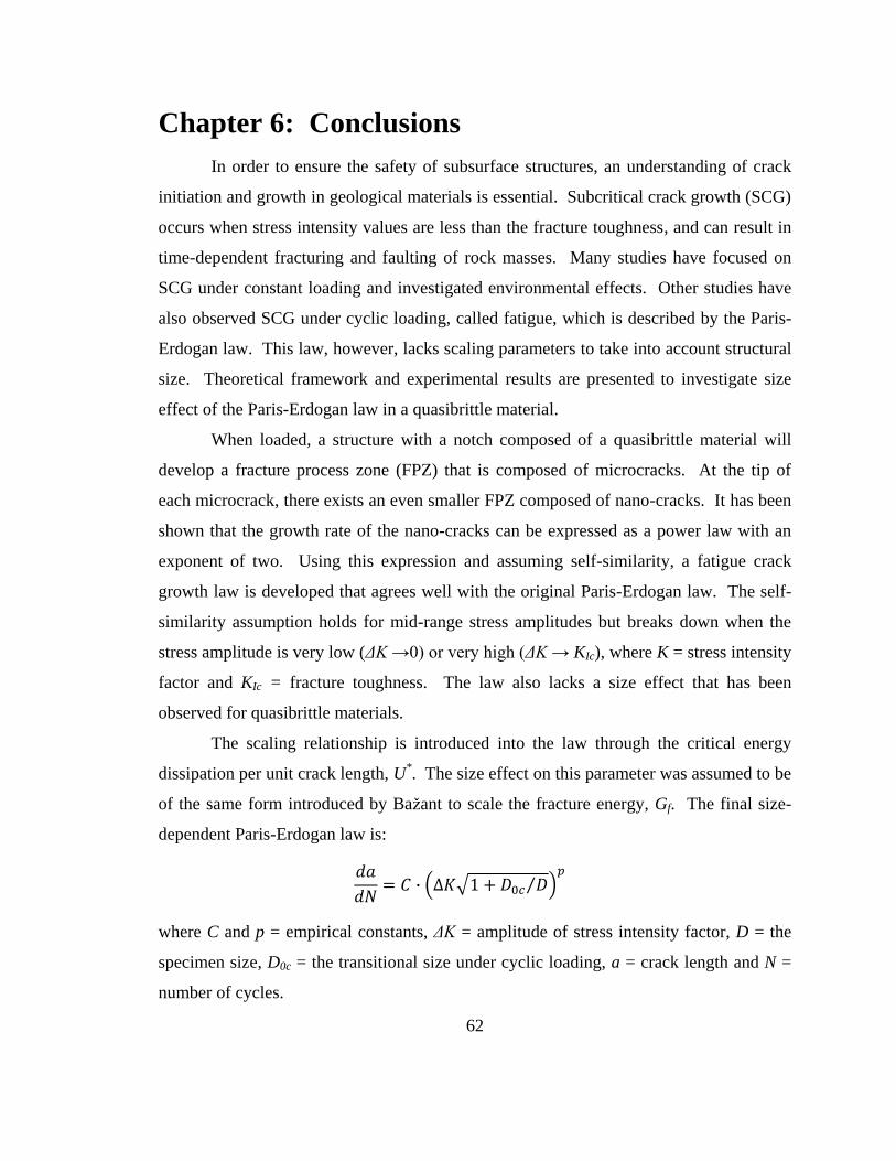
62

Chapter 6: Conclusions

In order to ensure the safety of subsurface structures, an understanding of crack

initiation and growth in geological materials is essential. Subcritical crack growth (SCG)

occurs when stress intensity values are less than the fracture toughness, and can result in

time-dependent fracturing and faulting of rock masses. Many studies have focused on

SCG under constant loading and investigated environmental effects. Other studies have

also observed SCG under cyclic loading, called fatigue, which is described by the Paris-

Erdogan law. This law, however, lacks scaling parameters to take into account structural

size. Theoretical framework and experimental results are presented to investigate size

effect of the Paris-Erdogan law in a quasibrittle material.

When loaded, a structure with a notch composed of a quasibrittle material will

develop a fracture process zone (FPZ) that is composed of microcracks. At the tip of

each microcrack, there exists an even smaller FPZ composed of nano-cracks. It has been

shown that the growth rate of the nano-cracks can be expressed as a power law with an

exponent of two. Using this expression and assuming self-similarity, a fatigue crack

growth law is developed that agrees well with the original Paris-Erdogan law. The self-

similarity assumption holds for mid-range stress amplitudes but breaks down when the

stress amplitude is very low (ΔK →0) or very high (ΔK → KIc), where K = stress intensity

factor and KIc = fracture toughness. The law also lacks a size effect that has been

observed for quasibrittle materials.

The scaling relationship is introduced into the law through the critical energy

dissipation per unit crack length, U*. The size effect on this parameter was assumed to be

of the same form introduced by Bažant to scale the fracture energy, Gf. The final size-

dependent Paris-Erdogan law is:

( √ ⁄ )

where C and p = empirical constants, ΔK = amplitude of stress intensity factor, D = the

specimen size, D0c = the transitional size under cyclic loading, a = crack length and N =

number of cycles.

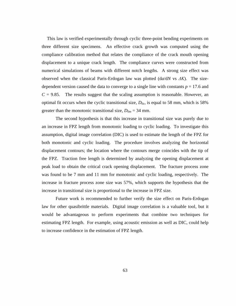
63

This law is verified experimentally through cyclic three-point bending experiments on

three different size specimens. An effective crack growth was computed using the

compliance calibration method that relates the compliance of the crack mouth opening

displacement to a unique crack length. The compliance curves were constructed from

numerical simulations of beams with different notch lengths. A strong size effect was

observed when the classical Paris-Erdogan law was plotted (da/dN vs ΔK). The size-

dependent version caused the data to converge to a single line with constants p = 17.6 and

C = 9.85. The results suggest that the scaling assumption is reasonable. However, an

optimal fit occurs when the cyclic transitional size, D0c, is equal to 58 mm, which is 58%

greater than the monotonic transitional size, D0m = 34 mm.

The second hypothesis is that this increase in transitional size was purely due to

an increase in FPZ length from monotonic loading to cyclic loading. To investigate this

assumption, digital image correlation (DIC) is used to estimate the length of the FPZ for

both monotonic and cyclic loading. The procedure involves analyzing the horizontal

displacement contours; the location where the contours merge coincides with the tip of

the FPZ. Traction free length is determined by analyzing the opening displacement at

peak load to obtain the critical crack opening displacement. The fracture process zone

was found to be 7 mm and 11 mm for monotonic and cyclic loading, respectively. The

increase in fracture process zone size was 57%, which supports the hypothesis that the

increase in transitional size is proportional to the increase in FPZ size.

Future work is recommended to further verify the size effect on Paris-Erdogan

law for other quasibrittle materials. Digital image correlation is a valuable tool, but it

would be advantageous to perform experiments that combine two techniques for

estimating FPZ length. For example, using acoustic emission as well as DIC, could help

to increase confidence in the estimation of FPZ length.

64

Chapter 7: References

[1] Suresh, S. Fatigue of Materials. Cambridge: Cambridge UP, 1998. Print.

[2] Hodgkinson, E.A. (1849) Report of commissioners appointed to enquire into the

application of iron to railway structures, Command Paper No. 1123. London: His

Majesty’s Stationery Office.

[3] Rankine, W.J.M. (1843) On the causes of unexpected breakage of the journals of

railway axles and the means of preventing such accidents by observing the law of

continuity in their construction. Proceeding of the Institute of Civil Engineering,

London 2, 105-108.

[4] Wöhler, A. (1860) Versuche über die festigkeit der eisenbahnwagenachsen.

Zeritschrift für Bauwesn 10; English Summary (1867). Engineering 4, 160-161.

[5] Fairburn, W. (1864) Experiments to determine the effect of impact, vibratory action,

and long continued changes of load on wrought iron girders. Philisophical

Transactions of the Royal Society, London 154, 311.

[6] Inglis, C.E. (1913) Stresses in a plate due to presence of cracks and sharp corners.

Transactions of the Institute of Naval Achitects 55, 219-241.

[7] Griffith, A.A. (1921) The phenomenon of rupture and flow in solids. Philisophical

Transaction of the Royal Society, London A221, 163-197.

[8] Irwin G.R. (1957) Analysis of stresses and strains near the end of a crack traversing a

plate. Journal of Applied Mechanics 24, 361-364.

[9] Paris, P.C., Gomez, M.P. & Anderson, W.P. (1961) A rational analytic theory of

fatigue. The Trend in Engineering 13, 9-14.

[10] Paris, P.C., Erdogan, F. (1963) A critical analysis of crack propagation laws.

Journal of Basic Engineering 85, 528-534.

[11] Docker, H., Marci, G. (1983) Threshold range and opening stress intensity factor in

fatigue. International Journal of Fatigue 5, 187-191.

[12] Kishimoto, H. Ueno, A. & Kawamoto, H. (1987) Fatigue crack propagation in

ceramics. Society of Materials Science Japan, 36, 1122-1127.

[13] Gao, Hua, Alagok, N., Brown, M.W. & Miller, K.J. (1985) Growth of fatigue cracks

under combined mode I and mode II loads. Multiaxial Fatigue, Special Technical

Publication 853, pp. 184-202. Philadelphia: American Society for testing and

Materials

65

[14] Ewart, L., Suresh, S. (1992) Elevated-temperature crack growth in polycrystalline

alumina under static and cyclic loads. Journal of Materials Science Letters 5,

774-778.

[15] El-Shabasy, A.B., Lewandowski, J.J. (2004) Effects of load ratio, R, and test

temperature on fatigue crack growth of fully pearlitic eutectoid steel.

International Journal of Fatigue 26, 305-309.

[16] Ritchie, R.O. (1988) Mechanisms of fatigue crack-propagation in metals, ceramics

and composites- role of crack tip shielding. Materials Science and Engineering

103, 15-28.

[17] Cook, R.F., Fairbanks, C.J. & Lawn, B.R. (1985) Microstucture-Strength Properties

in Ceramics .1. Effect of crack size on Toughness, and .2. Fatigue Relations.

Journal American Ceramic Society 68. 604-623.

[18] Hilsdorf, H.K. & Kesler, C.E. (1966) Fatigue Strength of Concrete under Varying

Flexural Stresses. ACI Journal Proceedings 63. 1059-1075.

[19] Atkinson, B.K. (1982). Subcritical crack-propagation in rocks – theory, experimental

results and applications. Journal of Structural Geology. 4, 41–56.

[20] Kilburn, C.R.J., Voight, B. (1998) Slow rock fracture as eruption precursor at

Soufriere Hills volcano. Geophysics Research Letters. 25, 3665–3668.

[21] Waza, T., Kurita, K., Mizutani, H., (1980) The effect of water on the subcritical

crack growth in silicate rocks. Tectonophysics 67, 25–34.

[22] Nara, Y., Takada, M., Igarashi, T., Hiroyoshi, N., Kaneko, K., (2009) Subcritical

crack growth in rocks in an aqueous environment. Exploration Geophysics. 40,

163–171.

[23] Nara, Y., Hiroyoshi, N., Yoneda, T., Kaneko, K., (2010) Effect of temperature and

relative humidity on subcritical crack growth in igneous rock. International

Journal of Rock Mechanics and Mining Sciences, 47, 640–646.

[24] Nara, Y., Morimoto, K., Hiroyoshi, N., Yoneda, T., Kaneko, K., Benson, P.M.

(2012) Influence of relative humidity on fracture toughness of rock:

Implicationsfor subcritical crack growth. International Journal of Solids and

Structures, 49, 2471-2481.

[25] Bažant, Z.P., Planas, J., (1998). Fracture and size effect in concrete and other

quasibrittle materials. CRCPress.

[26] Bažant, Z. P. (1984). Size effect in blunt fracture: concrete rock, metal. Journal of

Engineering Mechanics, Vol. 110, 518-535.

66

[27] Barenblatt G.I. (1959) The formation of equilibriujm crack during britlle fracture –

general ideas and hypotheses, azially-symmetric cracks. Journal of Applied

Mathematics and Mechanics, 23, 434-444.

[28] Dugdale D.W. (1960) Yielding of steel sheets containing slits. Journal of the

Mechanics and Physics of Solids, 8, 59-68.

[29] Labuz, J.F., Biolzi, L., (1998) Characteristic strength of quasi-brittle materials.

International Journal of Solids and Structures, 35, 4191-4203.

[30] Lin, Q., Fakhimi, A., Haggerty, M., Labuz, J.F. (2009) Initiation of tensile and

mixed-mode facture in sadstone. International Journal of Rock Mechanics and

Mining Sciences,46, 489-497.

[31] Lin, Q., Labuz, J. F. (2013) Fracture of sandstone characterized by digital image

correlation. International Journal of Rock Mechanics and Mining Sciences.

[32] Yamaguchi,I. (1981) Speckle Displacement and Decorrelation in the Diffraction and

Image Fields for Small Object Deformation. International Journal of Optics. Vol.

28. Issue 10. 1359-1376.

[33] Peters, W.H., Ranson, W.F. (1982) Digital imaging techniques in experimental stress

analysis. Optical Engineering 21 (3), 427-31.

[34] Sutton, M.A., Wolters, W.J., Peters, W.H., Ranson, W.A, McNeill, S.R. (1983)

Determination of displacements using an improved digital correlation method.

Image and Vision Computing 1 (3), 133-139.

[35] Bruck, H.A., McNeill, S.R., Sutton, M.A., Peters, W.H. (1989) Digital image

correlation using Newton-Raphson method of partial differential correction.

Experimental Mechanics. Volume 29. Issue 3. 261-267.

[36] Chen, D.J., Chiang, Y.S. Tan, Don, D.S, (1993) Digital speckle-displacement

measurement using a complex spectrum method. Applied Optics, Vol. 32, Issue

11. 1839-1849.

[37] Sutton, M.A., McNeill, S.R., Jang, J., Babai, M. (1988) Effects Of Subpixel Image

Restoration On Digital Correlation Error Estimates. Optical Engineering 27(10)

271070.

[38] Schreier, H.W., Braasch, J.R., Sutton, M.A. (2000) Systematic errors in digital

image correlation caused by intensity interpolation. Optical Engineering 39(11)

2915-2921.

[39] Peters, W.H., Ranson, W.F., Sutton, M.A., Chu, T.C., Anderson, J. (1983)

Application of digital correlation methods to rigid body mechanics. Optical

Engineering 22(6) 226738.

67

[40] Chu, T.C., Ranson, W.F., Sutton, M.A., (1985) Applications of digital-image-

correlation techniques to experimental mechanics. Experimental Mechanics,

Vol25, Issue 3, 232-244.

[41] StrainMaster. (2007) Advanced image based Tools for Optical Defromation and

Strain Measurement [Brochure]. Ypsilanti, MI: LaVision Inc.

[42] Le, J.L., Bažant, Z.P., Bažant, M.Z., (2011) Unified nano-mechanics based

probabilistic theory of quasibrittle and brittle structures: I. Strength, static crack

growth, lifetime and scaling. Journal of the Mechanics and Physics of Solids. Vol

59, Issue 7, 1291-1321.

[43] Bažant, Z. P., Xu, K. (1991) Size effect in fatigue fracture of concrete. ACI

Materials Journal, 88(4), 390-99.

[44] Ogawa, T., (1995) Fatigue crack growth of monolithic and composite ceramics.

Cyclic Fatigue in Ceramics. Elsevier Science B. V. and The society of Materials

Science, Japan. 167-188.

[45] Studarta, A.R., Filser, F., Kochera, P., Gaukler, L.J., (2007) Fatigue of zirconia

under cyclic loadin in water and its implications for the design of dental bridges.

Dental Materials. 23, 106-114.

[46] Andersons, J., Hojo, M., Ochiai, S., (2004) Emperical model for stress ratio effect on

fatigue delamination growth rate in composite laminates. International Journal of

Fatigue 26,567-604.

[47] Swartz, S. E., Hu, K. K. and Jones, G. L. (1978) Compliance monitoring of crack

growth in concrete. Journal of Engineering Mechanics Division –ASCE 104. 789-

800.

[48] Pearson, S. (1975) Initiation of fatigue cracks in commercial aluminum alloys and

the subsequent propagation of very short cracks. Engineering Fracture Mechanics

7, 235-247.

[49] Lankford, J. (1983) The effect of environment on the growth of small fatigue cracks.

Fatigue of Engineering Materials and Structures 5, 233-248.

[50] Tanaka, K. Hojo, M., Nakai, Y. (1983) Crack initiation and early propagation in 3%

silicon iron. Fatigue Mechanisms: Advances in Quantitative Measurement of

Fatigue Damage, Special Technical Publication 881, 207-232. Philidelphia:

American society for Testing and Materials.