1

Supporting Information for

Single-Ion Magnet Behavior in Heptacoordinated Fe(II) Complexes: On the Importance of Supramolecular Organization

Arun Kumar Bar,ab Céline Pichon,ab Nayanmoni Gogoi,ab Carine Duhayon,ab S. Ramasesha,c and Jean-Pascal Sutter*,ab

a CNRS, LCC, 205 Route de Narbonne, F-31077 Toulouse, France.

b Université de Toulouse, UPS, INPT, LCC, F-31007 Toulouse, France. c Indian Institute of Science, Bangalore 560012, India

E-mail : sutter@lcc-toulouse.fr

Experimental Section

Materials and methods:

All reagents and solvents used for the syntheses were used as received from commercial sources. All the solvents used in the air-sensitive reactions were distilled under anaerobic condition and degased by following the freeze and thaw method prior to use. The organic ligand H2DAPBH1 was synthesized following reported procedures. Fourier transform infrared (FT-IR) spectroscopy was performed with a Perkin–Elmer spectrum GX 2000 FT-IR spectrometer. Elemental analyses were performed with a Perkin–Elmer 2400 series II instrument.

Magnetic susceptibility measurements were carried out with a Quantum Design MPMS-5S SQUID susceptometer. The magnetic measurements were performed on freshly filtered polycrystalline materials. The polycrystalline powders were mixed with grease and put in gelatin capsules. All the magnetic samples associated with Fe(II) metal ion were prepared under N2 atmosphere. dc measurements were conducted from 300 to 2 K at 1 kOe and the data were corrected for the diamagnetic contribution of the sample holder, grease and sample by using Pascal’s tables.2 The field dependences of the magnetization were measured at several temperatures between 2 and 10 K with dc magnetic field up to 5 T. Preliminary ac susceptibility experiments for 1 and 2 were performed at various frequencies ranging from 1 to 1500 Hz with an ac field amplitude of 3 Oe. ac susceptibility was investigated under an oscillating ac field of 3 Oe over the frequency range of 1 to 1500 Hz. High frequency ac experiments were carried out on a Quantum Design PPMS under an oscillating ac field of 3 Oe over the frequency range of 100 to 10000 Hz.

Mössbauer measurements were recorded at 80 K using an MD 306 Oxford cryostat on a constant acceleration conventional spectrometer with a 50 mCi source of 57Fe (Rh matrix).

1 T. J. Giordano, G. J. Palenik, R. C. Palenik, D. A. Sullivan, Inorg. Chem., 1979, 18, 2445. 2 O. Kahn, Molecular Magnetism, VCH, Weinheim, 1993.

Electronic Supplementary Material (ESI) for ChemComm.This journal is © The Royal Society of Chemistry 2015

2

The absorber was a powdered sample enclosed in a 20 mm diameter cylindrical, plastic sample holder, the size of which had been determined to optimize the absorption. A least-squares computer program was used to fit the Mössbauer parameters and determine their standard deviations (given in parentheses). Isomer shift values (δ) are relative to iron foil at 293 K.

X-ray crystallographic studies: Single crystals suitable for X-ray diffraction were coated with paratone oil and mounted onto the goniometer. The X-ray crystallographic data were obtained at low temperature from a Gemini Oxford Diffraction (CuKα radiation source) or an Apex2 Bruker diffractometer (MoKα radiation source) and equipped with an Oxford Cryosystem. The structures have been solved by direct methods using Shelxs or Superflip and refined by means of least-square procedures on F using the PC version of the program CRYSTALS.3 The scattering factors for all the atoms were used as listed in the International Tables for X-ray Crystallography.4 Absorption correction was performed using a multi-scan procedure. All non-hydrogen atoms were refined anisotropically. When it was possible, the H atoms were located in a difference map, but those attached to carbon atoms were repositioned geometrically. The H atoms were initially refined with soft restraints on the bond lengths and angles to regularise their geometry and U~iso~(H) (in the range 1.2-1.5 times U~eq~ of the parent atom), after which the positions were refined with riding constraints. Structures 1 and 3 were disordered. For compound 1, three F atoms were disordered on 2 sites (0.5 : 0.5 occupancy). Moreover, for structure 3 restraints (using the command SAME) were applied for the two parts of the disordered phenyl (0.55 : 0.45 occupancy). For compound 2, the detected electron densities suggested the presence of a half occupancy methanol molecule with high thermal motion The molecule appears disordered over several positions that can be approximated by 4 oxygen positions with occupancies 0.3, 0.3, 0.3, and 0.1. Tentative refinement of the MeOH molecule lead to odd C-O distances, therefore we decided to remove this residual density using the SQUEEZE facility from PLATON.

Computational studies: Single point energy and spin density distribution were computed for 1 and 2 using TD-DFT on GAUSSIAN-095 platform utilizing hybrid UB3LYP6 basis functions with mixed basis sets: 6-31G*7 for all non-metal elements and the small-core Hay-Wadt pseudopotential (indicated in the Gaussian code as LANL2DZ)8 for Fe. The mixing of d and p as well as HOMO and LUMO orbitals were allowed. The crystallographic coordinates of the di-cationic moiety [Fe(H2DAPBH)(H2O)(MeOH)]2+ for 1 and of the neutral moiety [Fe(H2DAPBH)Cl2] for 2 were used for the calculations (Table SI11-12). The S**2

3 P. W. Betteridge, J. R. Carruthers, R. I. Cooper, K. Prout, D. J. Watkin, J. Appl. Crystallogr., 2003, 36, 1487. 4 International Tables for X-ray Crystallography, Vol. IV, Kynoch Press, Birmingham, England, 1974. 5 M. J. Frisch, G. W. Trucks, H. B. Schlegel, G. E. Scuseria, M. A. Robb, J. R. Cheeseman, G. Scalmani, V. Barone, B. Mennucci, G. A. Petersson, H. Nakatsuji, M. Caricato, X. Li, H. P. Hratchian, A. F. Izmaylov, J. Bloino, G. Zheng, J. L. Sonnenberg, M. Hada, M. Ehara, K. Toyota, R. Fukuda, J. Hasegawa, M. Ishida, T. Nakajima, Y. Honda, O. Kitao, H. Nakai, T. Vreven, J. A. Montgomery, Jr., J. E. Peralta, F. Ogliaro, M. Bearpark, J. J. Heyd, E. Brothers, K. N. Kudin, V. N. Staroverov, R. Kobayashi, J. Normand, K. Raghavachari, A. B. Rendell, J. C., S. S. Iyengar, J. Tomasi, M. Cossi, N. Rega, M. J. Millam, M. Klene, J. E. Knox, J. B. Cross, V. Bakken, C. Adamo, J. Jaramillo, R. Gomperts, R. E. Stratmann, O. Yazyev, A. J. Austin, R. Cammi, C. Pomelli, J. W. Ochterski, R. L. Martin, K. Morokuma, V. G. Zakrzewski, G. A. Voth, P. Salvador, J. J. Dannenberg, S. Dapprich, A. D. Daniels, Ö. Farkas, J. B. Foresman, J. V. Ortiz, J. Cioslowski and D. J. Fox, Gaussian 09; Gaussian, Inc., Wallingford CT, 2009. 6 A. D. J. Becke, J. Chem. Phys., 1993, 98, 5648. 7 T. H. J. Dunning, P. J. Hay, In Modern Theoretical Chemistry; Schaefer, H. F., III, Ed.; Plenum: New York, 1976; Vol. 3. 8 P. J. Hay, R. J. Wadt, Chem. Phys. Chem., 1985, 82, 299.

3

values in the output files after normal termination were cross-checked. The S**2 values after annihilations are found to be 6.0000 for 1 and 6.0002 for 2 and thus excluding the spin contaminations. The estimated spin densities are Mulliken atomic spin densities (Table SI13-14). The spin density maps were drawn using GassView4.1 software9 and are presented in 4×10-4 μB Å3 isosurface (Figure SI5).

9 A. E. Frisch, R. D. Dennington, T. A. Keith, J. Millam, A. B. Nielsen, A. J. Holder, J. Hiscocks, Gaussian, Inc., Wallingford CT, 2003.

4

Synthesis:

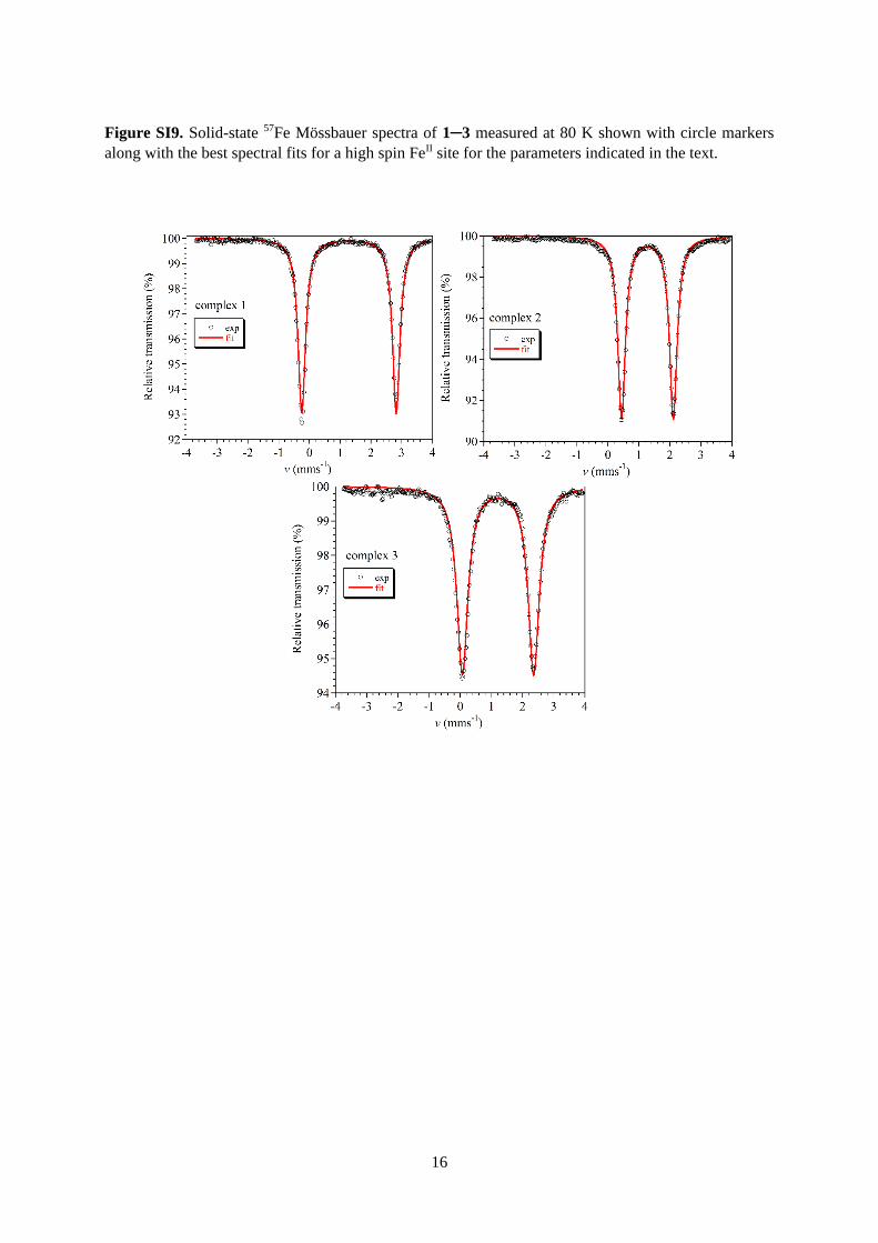
[Fe(H2DAPBH)(H2O)(MeOH)] 2MeOH 2BF4, 1: The reaction was carried out at room temperature under N2 atmosphere using standard Schlenk line technique. In a 50 mL round bottom Schlenk flask, 675 mg (2 mmol) of Fe(BF4)2.6H2O was dissolved in 20 mL of degased MeOH yielding a colorless solution. In a 100 mL Schlenk tube, 2 mmol of the corresponding organic ligand H2DAPBH (800 mg) in 60 mL of degased MeOH gave a milky slurry. The methanol solution of Fe(II) was then slowly added with a syringe into the slurry. The deep blue solution was stirred at room temperature for 6 h followed by filtering through a frit under N2 atmosphere into a 250 mL Schlenk tube. The filtrate was concentrated under vacuum to ~150 mL and ca.100 mL of degased diethyl ether was layered over it for slow diffusion. The whole set up was kept undisturbed under inert atmosphere for 10−14 days until the complex crystallized out rendering the mother liquor almost colorless. The polycrystalline solid was filtered off the solvent mixture through frit under N2 atmosphere, washed twice with 10 mL portions of degased diethyl ether and finally dried under low vacuum to obtain polycrystalline dark blue solid (905 mg; 67 %). Good quality single crystals suitable for X-ray diffraction were picked up before filtering off the crystalline material. IR (cm-1): υC=O = 1627 (vs) and 1578 (s); υC=N = 1522 (vs). Elemental analysis (%) calcd. for C24H27N5O4B2F8Fe: C 42.46; H 4.01; N 10.31; found: C 41.96; H 4.07; N 10.22. Mössbauer: one symmetric doublet: δ = 1.289(12) mm/s; ∆ = 3.0728(23) mm/s.

[Fe(H2DAPBH)Cl2] 0.5MeOH, 2: (Adapted from a reported procedure10) In a 50 mL round bottom Schlenk flask, 397.7 mg (2 mmol) of FeCl2.4H2O was dissolved in 20 mL of degased MeOH yielding a greenish yellow solution. In a 100 mL Schlenk tube 2 mmol of the corresponding organic ligand (800 mg of H2DAPBH) in 60 mL of degased MeOH gave a milky slurry. The methanol solution of FeCl2 was then slowly added with a syringe into the slurry. The deep blue solution was stirred at room temperature for 6 h followed by filtering through a frit under N2 atmosphere into a 250 mL Schlenk tube. The filtrate was concentrated under vacuum to ~150 mL and ~100 mL of degased diethyl ether was layered over it for slow diffusion. The whole set up was kept undisturbed under inert atmosphere for 10−14 days until the complex crystallized out rendering the mother liquor almost colorless followed by filtration off the solvent mixture through frit under N2 atmosphere. The isolated solid was washed twice with 10 mL portions of degased diethyl ether followed by drying under low vacuum to obtain polycrystalline dark blue solid; mass (yield): 810 mg (73 %). Good quality single crystals suitable for X-ray diffraction were picked up before filtering off the crystalline material. IR (cm-1): υC=O = 1624 (vs) and 1579 (s); υC=N = 1522 (vs). Elemental analysis (%) calcd. for C23H21N5O2Cl2Fe: C 52.50; H 4.02; N 13.31; found: C 52.60; H 4.07; N 13.28. Mössbauer: one symmetric doublet: δ = 1.27657(87) mm/s; ∆ = 1.6687(17) mm/s.

[Fe(H2DAPBH){Ni(CN)4}]∞, 3: A 100 mL columnar Schlenk tube was charged with 241 mg (1 mmol) of K2Ni(CN)4 in 15 mL of water under N2 atmosphere. Additional 5 mL of water was layered over the aqueous solution of K2Ni(CN)4, and finally a methanol solution of 1

10 A. S. M. Al-Shihri, J. R. Dilworth, S. D. Howe, J. Silver, R. M. Thompson, J. Davies, D. C. Povey, Polyhedron, 1993, 12, 2297.

5

mmol (558 mg) of the complex 2 was slowly layered on top. The whole set up was kept

undisturbed under N2 atmosphere. Slow interdiffusion of these two solutions resulted in pale

blue crystals. After 2−3 days, the whole reaction mixture was mechanically stirred and was

filtered off through frit under N2 atmosphere followed by drying under vacuum to obtain a

polycrystalline dark blue solid (557 mg; 90 %). Desirable single crystals required for the X-

ray data collections were picked up from these crystals prior to mechanical stirring. IR (cm-1):

C=O = 1631 (vs) and 1579 (m); C=N = 1526 (vs); CN = 2134 (s). Elemental analysis (%)

calcd. for C27H21N9O2FeNi: C 52.47; H 3.42; N 20.40; Found: C 52.34; H 3.49; N 20.18.

Mössbauer: single symmetric doublet; site population 100 %; = 1.2138(19) mm/s; ∆ =

2.2889(38) mm/s.

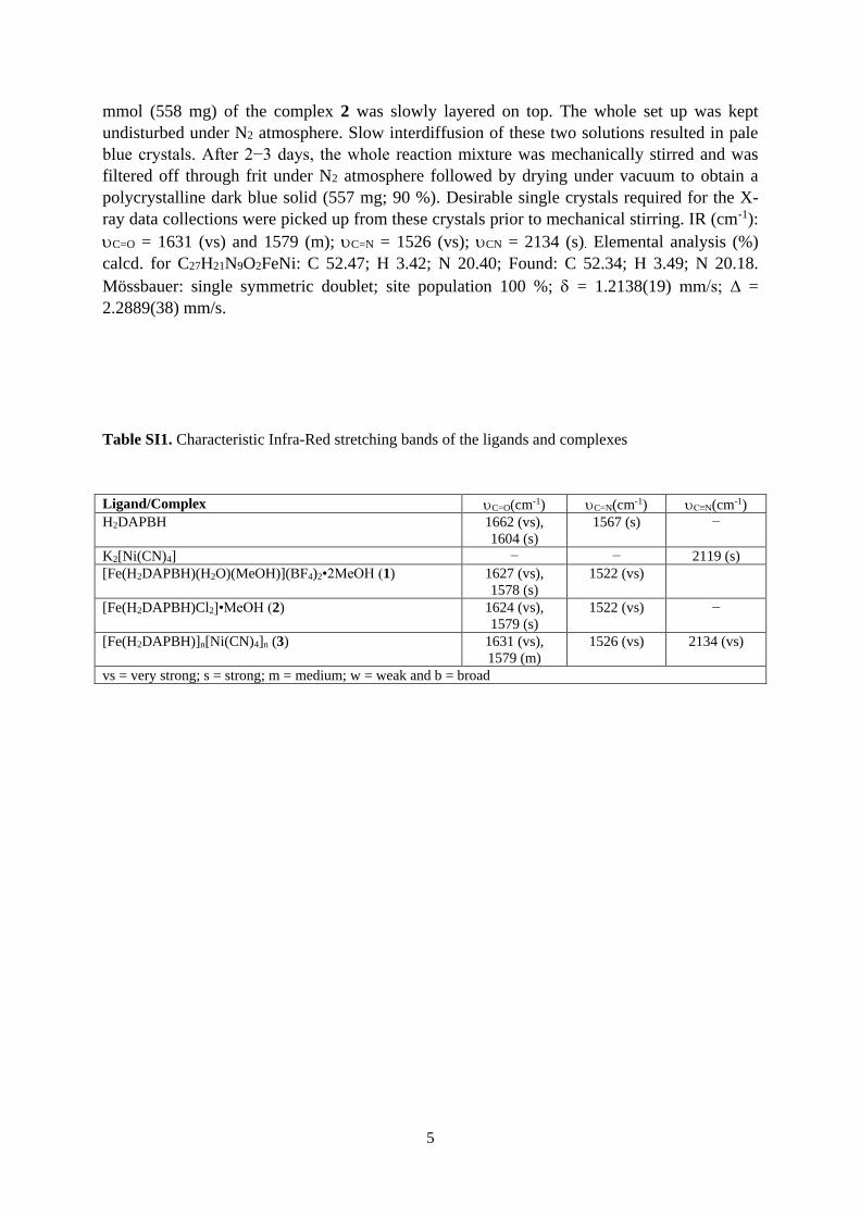
Table SI1. Characteristic Infra-Red stretching bands of the ligands and complexes

Ligand/Complex C=O(cm-1) C=N(cm-1) C≡N(cm-1)

H2DAPBH 1662 (vs),

1604 (s)

1567 (s) −

K2[Ni(CN)4] − − 2119 (s)

[Fe(H2DAPBH)(H2O)(MeOH)](BF4)2•2MeOH (1) 1627 (vs),

1578 (s)

1522 (vs)

[Fe(H2DAPBH)Cl2]•MeOH (2) 1624 (vs),

1579 (s)

1522 (vs) −

[Fe(H2DAPBH)]n[Ni(CN)4]n (3) 1631 (vs),

1579 (m)

1526 (vs) 2134 (vs)

vs = very strong; s = strong; m = medium; w = weak and b = broad

6

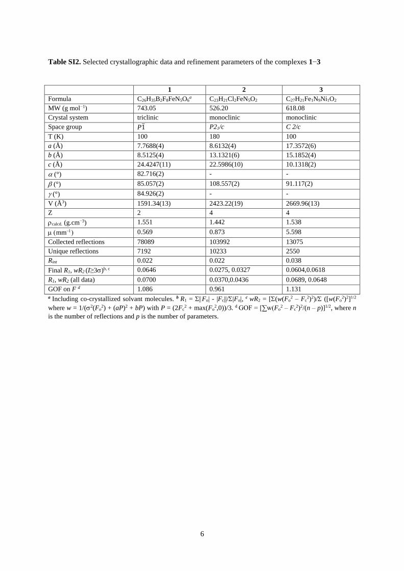
Table SI2. Selected crystallographic data and refinement parameters of the complexes 1−3

1 2 3

Formula C26H35B2F8FeN5O6a C23H21Cl2FeN5O2 C27H21Fe1N9Ni1O2

MW (g mol−1) 743.05 526.20 618.08

Crystal system triclinic monoclinic monoclinic

Space group P1̅ P21/c C 2/c

T (K) 100 180 100

a (Å) 7.7688(4) 8.6132(4) 17.3572(6)

b (Å) 8.5125(4) 13.1321(6) 15.1852(4)

c (Å) 24.4247(11) 22.5986(10) 10.1318(2)

(°) 82.716(2) - -

(°) 85.057(2) 108.557(2) 91.117(2)

(°) 84.926(2) - -

V (Å3) 1591.34(13) 2423.22(19) 2669.96(13)

Z 2 4 4

calcd. (g.cm−3) 1.551 1.442 1.538

mm 0.569 0.873 5.598

Collected reflections 78089 103992 13075

Unique reflections 7192 10233 2550

Rint 0.022 0.022 0.038

Final R1, wR2 (I≥3)b, c 0.0646 0.0275, 0.0327 0.0604,0.0618

R1, wR2 (all data) 0.0700 0.0370,0.0436 0.0689, 0.0648

GOF on F d 1.086 0.961 1.131 a Including co-crystallized solvant molecules. b R1 = Fo| - |Fc||/|Fo|, c wR2 = [(w(Fo

2 – Fc2)2)/ ([w(Fo

2)2]1/2

where w = 1/(2(Fo2) + (aP)2 + bP) with P = (2Fc

2 + max(Fo2,0))/3. d GOF = [∑w(Fo

2 – Fc2)2/(n – p)]1/2, where n

is the number of reflections and p is the number of parameters.

7

Figure SI1. View of the crystal packing of 1 along the crystallographic b axis. Color codes: yellow =

Fe; green = F, red = O; blue = N, dark grey = C and pink = B. The H atoms and interstitial solvent

molecules are omitted for clarity. Some of the F atoms of the BF4- ions have thermal disorder. Only

one position of the disordered F atoms is shown for clarity.

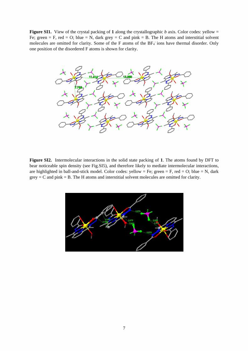
Figure SI2. Intermolecular interactions in the solid state packing of 1. The atoms found by DFT to

bear noticeable spin density (see Fig.SI5), and therefore likely to mediate intermolecular interactions,

are highlighted in ball-and-stick model. Color codes: yellow = Fe; green = F, red = O; blue = N, dark

grey = C and pink = B. The H atoms and interstitial solvent molecules are omitted for clarity.

8

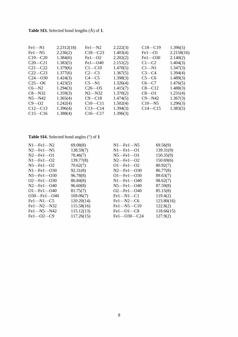
Table SI3. Selected bond lengths (Å) of 1.

Fe1—N1 2.2312(18) Fe1—N2 2.222(3) C18—C19 1.396(5)

Fe1—N5 2.236(2) C18—C23 1.403(4) Fe1—O1 2.2158(16)

C19—C20 1.384(6) Fe1—O2 2.202(2) Fe1—O30 2.140(2)

C20—C21 1.383(5) Fe1—O40 2.151(2) C1—C2 1.404(3)

C21—C22 1.379(6) C1—C10 1.470(5) C1—N1 1.347(3)

C22—C23 1.377(6) C2—C3 1.367(5) C3—C4 1.394(4)

C24—O30 1.424(3) C4—C5 1.398(3) C5—C6 1.489(3)

C25—O6 1.423(5) C5—N1 1.326(4) C6—C7 1.476(5)

C6—N2 1.294(3) C26—O5 1.415(7) C8—C12 1.488(3)

C8—N32 1.359(3) N2—N32 1.370(2) C8—O1 1.231(4)

N5—N42 1.365(4) C9—C18 1.474(5) C9—N42 1.367(3)

C9—O2 1.242(4) C10—C11 1.502(4) C10—N5 1.296(3)

C12—C13 1.396(4) C13—C14 1.394(3) C14—C15 1.383(5)

C15—C16 1.388(4) C16—C17 1.396(3)

Table SI4. Selected bond angles (°) of 1

N1—Fe1—N2 69.08(8) N1—Fe1—N5 69.56(9)

N2—Fe1—N5 138.59(7) N1—Fe1—O1 139.31(9)

N2—Fe1—O1 70.46(7) N5—Fe1—O1 150.35(9)

N1—Fe1—O2 139.77(8) N2—Fe1—O2 150.69(6)

N5—Fe1—O2 70.62(7) O1—Fe1—O2 80.92(7)

N1—Fe1—O30 92.31(8) N2—Fe1—O30 86.77(8)

N5—Fe1—O30 96.78(8) O1—Fe1—O30 89.63(7)

O2—Fe1—O30 86.84(8) N1—Fe1—O40 98.62(7)

N2—Fe1—O40 96.60(8) N5—Fe1—O40 87.59(8)

O1—Fe1—O40 81.75(7) O2—Fe1—O40 85.15(8)

O30—Fe1—O40 169.06(7) Fe1—N1—C1 119.4(2)

Fe1—N1—C5 120.20(14) Fe1—N2—C6 123.80(16)

Fe1—N2—N32 115.58(16) Fe1—N5—C10 122.8(2)

Fe1—N5—N42 115.12(13) Fe1—O1—C8 118.66(15)

Fe1—O2—C9 117.26(15) Fe1—O30—C24 127.9(2)

9

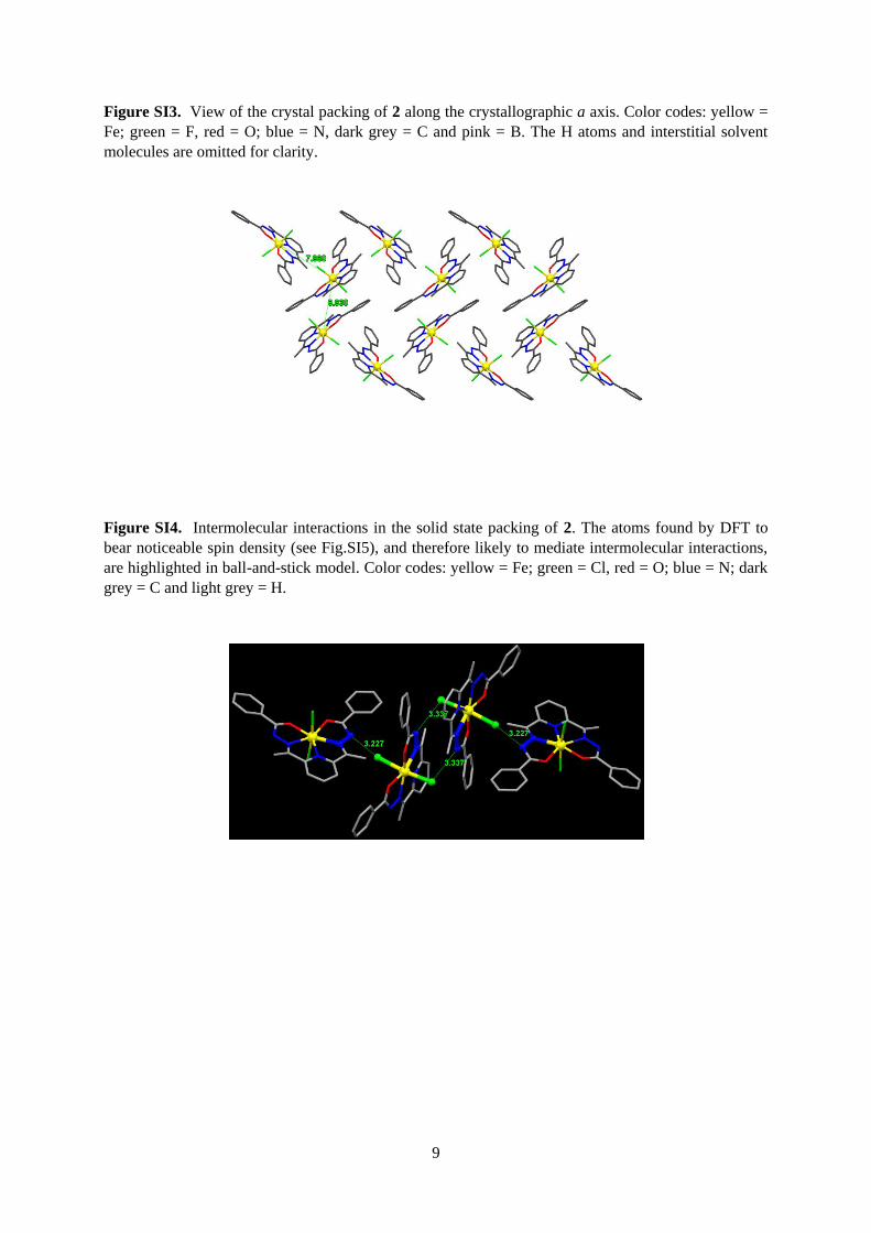
Figure SI3. View of the crystal packing of 2 along the crystallographic a axis. Color codes: yellow =

Fe; green = F, red = O; blue = N, dark grey = C and pink = B. The H atoms and interstitial solvent

molecules are omitted for clarity.

Figure SI4. Intermolecular interactions in the solid state packing of 2. The atoms found by DFT to

bear noticeable spin density (see Fig.SI5), and therefore likely to mediate intermolecular interactions,

are highlighted in ball-and-stick model. Color codes: yellow = Fe; green = Cl, red = O; blue = N; dark

grey = C and light grey = H.

10

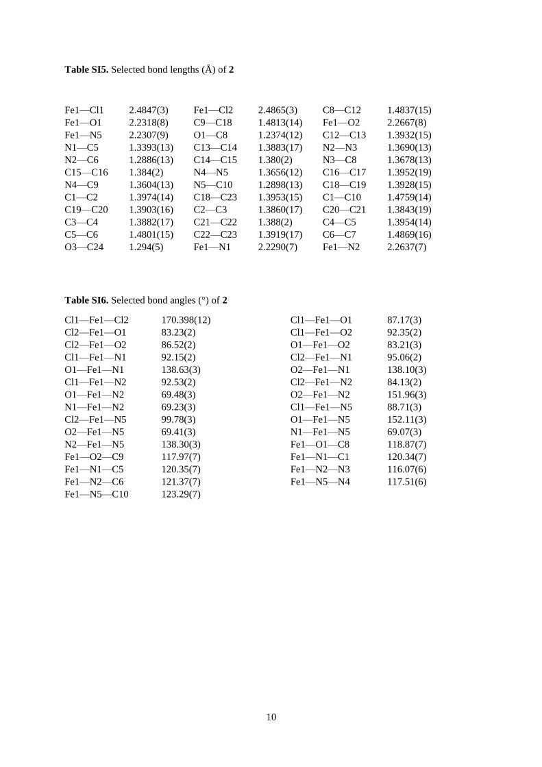
Table SI5. Selected bond lengths (Å) of 2

Fe1—Cl1 2.4847(3) Fe1—Cl2 2.4865(3) C8—C12 1.4837(15)

Fe1—O1 2.2318(8) C9—C18 1.4813(14) Fe1—O2 2.2667(8)

Fe1—N5 2.2307(9) O1—C8 1.2374(12) C12—C13 1.3932(15)

N1—C5 1.3393(13) C13—C14 1.3883(17) N2—N3 1.3690(13)

N2—C6 1.2886(13) C14—C15 1.380(2) N3—C8 1.3678(13)

C15—C16 1.384(2) N4—N5 1.3656(12) C16—C17 1.3952(19)

N4—C9 1.3604(13) N5—C10 1.2898(13) C18—C19 1.3928(15)

C1—C2 1.3974(14) C18—C23 1.3953(15) C1—C10 1.4759(14)

C19—C20 1.3903(16) C2—C3 1.3860(17) C20—C21 1.3843(19)

C3—C4 1.3882(17) C21—C22 1.388(2) C4—C5 1.3954(14)

C5—C6 1.4801(15) C22—C23 1.3919(17) C6—C7 1.4869(16)

O3—C24 1.294(5) Fe1—N1 2.2290(7) Fe1—N2 2.2637(7)

Table SI6. Selected bond angles (°) of 2

Cl1—Fe1—Cl2 170.398(12) Cl1—Fe1—O1 87.17(3)

Cl2—Fe1—O1 83.23(2) Cl1—Fe1—O2 92.35(2)

Cl2—Fe1—O2 86.52(2) O1—Fe1—O2 83.21(3)

Cl1—Fe1—N1 92.15(2) Cl2—Fe1—N1 95.06(2)

O1—Fe1—N1 138.63(3) O2—Fe1—N1 138.10(3)

Cl1—Fe1—N2 92.53(2) Cl2—Fe1—N2 84.13(2)

O1—Fe1—N2 69.48(3) O2—Fe1—N2 151.96(3)

N1—Fe1—N2 69.23(3) Cl1—Fe1—N5 88.71(3)

Cl2—Fe1—N5 99.78(3) O1—Fe1—N5 152.11(3)

O2—Fe1—N5 69.41(3) N1—Fe1—N5 69.07(3)

N2—Fe1—N5 138.30(3) Fe1—O1—C8 118.87(7)

Fe1—O2—C9 117.97(7) Fe1—N1—C1 120.34(7)

Fe1—N1—C5 120.35(7) Fe1—N2—N3 116.07(6)

Fe1—N2—C6 121.37(7) Fe1—N5—N4 117.51(6)

Fe1—N5—C10 123.29(7)

11

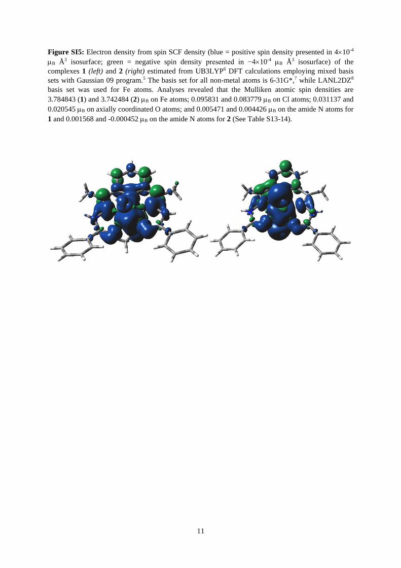
Figure SI5: Electron density from spin SCF density (blue = positive spin density presented in 410-4

B Å3 isosurface; green = negative spin density presented in −410-4 B Å3 isosurface) of the

complexes 1 (left) and 2 (right) estimated from UB3LYP6 DFT calculations employing mixed basis

sets with Gaussian 09 program.5 The basis set for all non-metal atoms is 6-31G*,7 while LANL2DZ8

basis set was used for Fe atoms. Analyses revealed that the Mulliken atomic spin densities are

3.784843 (1) and 3.742484 (2) B on Fe atoms; 0.095831 and 0.083779 B on Cl atoms; 0.031137 and

0.020545 B on axially coordinated O atoms; and 0.005471 and 0.004426 B on the amide N atoms for

1 and 0.001568 and -0.000452 B on the amide N atoms for 2 (See Table S13-14).

12

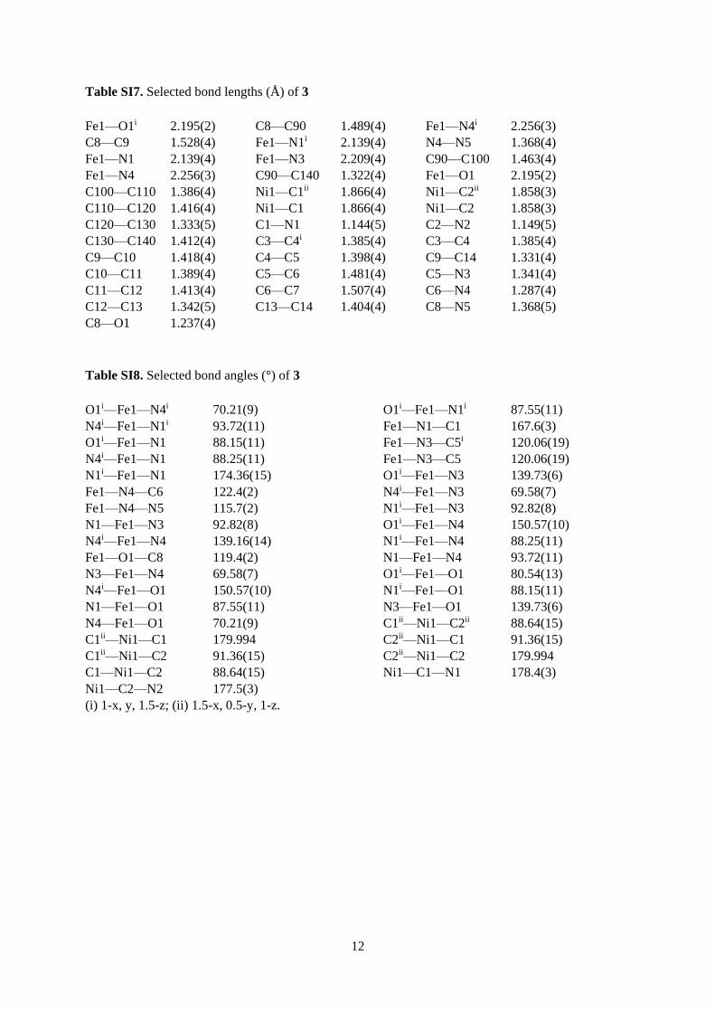
Table SI7. Selected bond lengths (Å) of 3

Fe1—O1i 2.195(2) C8—C90 1.489(4) Fe1—N4i 2.256(3)

C8—C9 1.528(4) Fe1—N1i 2.139(4) N4—N5 1.368(4)

Fe1—N1 2.139(4) Fe1—N3 2.209(4) C90—C100 1.463(4)

Fe1—N4 2.256(3) C90—C140 1.322(4) Fe1—O1 2.195(2)

C100—C110 1.386(4) Ni1—C1ii 1.866(4) Ni1—C2ii 1.858(3)

C110—C120 1.416(4) Ni1—C1 1.866(4) Ni1—C2 1.858(3)

C120—C130 1.333(5) C1—N1 1.144(5) C2—N2 1.149(5)

C130—C140 1.412(4) C3—C4i 1.385(4) C3—C4 1.385(4)

C9—C10 1.418(4) C4—C5 1.398(4) C9—C14 1.331(4)

C10—C11 1.389(4) C5—C6 1.481(4) C5—N3 1.341(4)

C11—C12 1.413(4) C6—C7 1.507(4) C6—N4 1.287(4)

C12—C13 1.342(5) C13—C14 1.404(4) C8—N5 1.368(5)

C8—O1 1.237(4)

Table SI8. Selected bond angles (°) of 3

O1i—Fe1—N4i 70.21(9) O1i—Fe1—N1i 87.55(11)

N4i—Fe1—N1i 93.72(11) Fe1—N1—C1 167.6(3)

O1i—Fe1—N1 88.15(11) Fe1—N3—C5i 120.06(19)

N4i—Fe1—N1 88.25(11) Fe1—N3—C5 120.06(19)

N1i—Fe1—N1 174.36(15) O1i—Fe1—N3 139.73(6)

Fe1—N4—C6 122.4(2) N4i—Fe1—N3 69.58(7)

Fe1—N4—N5 115.7(2) N1i—Fe1—N3 92.82(8)

N1—Fe1—N3 92.82(8) O1i—Fe1—N4 150.57(10)

N4i—Fe1—N4 139.16(14) N1i—Fe1—N4 88.25(11)

Fe1—O1—C8 119.4(2) N1—Fe1—N4 93.72(11)

N3—Fe1—N4 69.58(7) O1i—Fe1—O1 80.54(13)

N4i—Fe1—O1 150.57(10) N1i—Fe1—O1 88.15(11)

N1—Fe1—O1 87.55(11) N3—Fe1—O1 139.73(6)

N4—Fe1—O1 70.21(9) C1ii—Ni1—C2ii 88.64(15)

C1ii—Ni1—C1 179.994 C2ii—Ni1—C1 91.36(15)

C1ii—Ni1—C2 91.36(15) C2ii—Ni1—C2 179.994

C1—Ni1—C2 88.64(15) Ni1—C1—N1 178.4(3)

Ni1—C2—N2 177.5(3)

(i) 1-x, y, 1.5-z; (ii) 1.5-x, 0.5-y, 1-z.

13

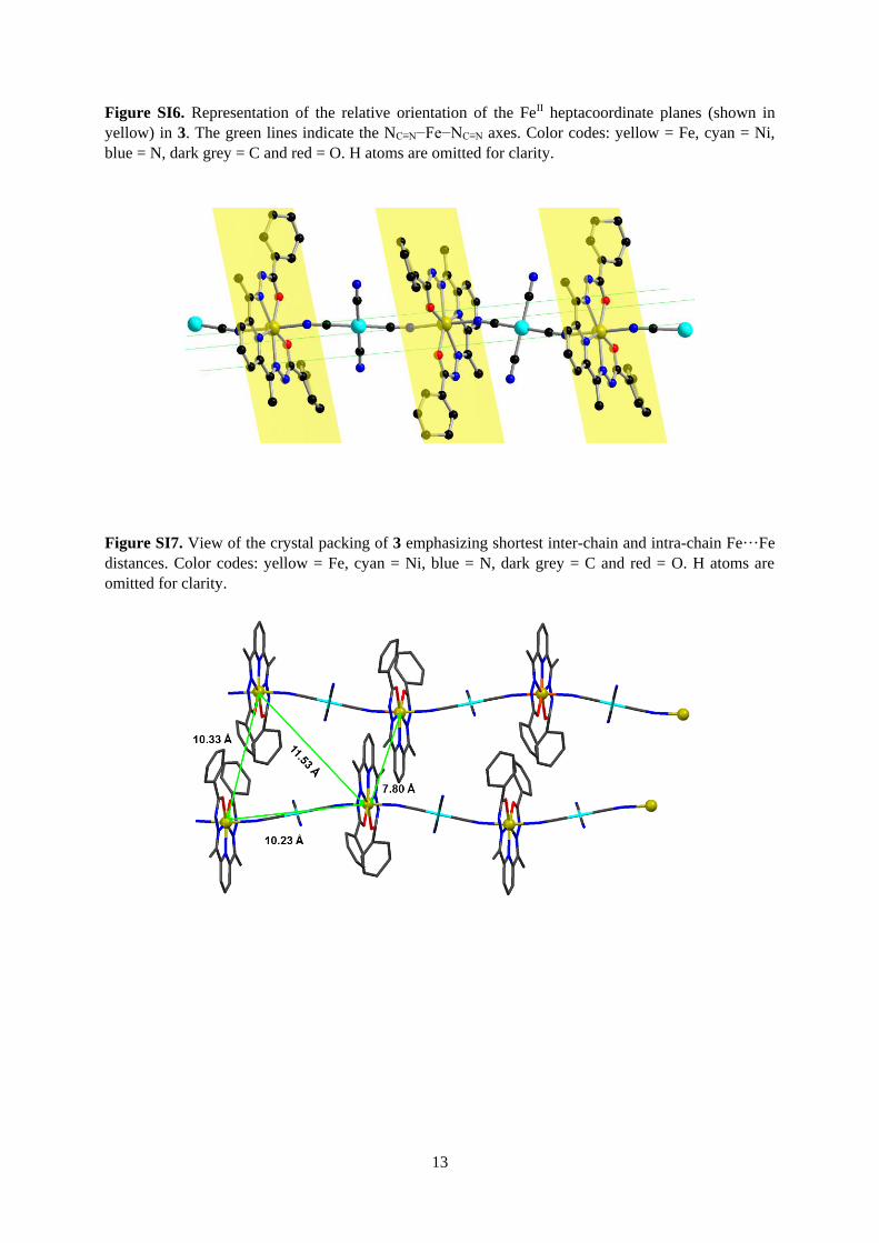
Figure SI6. Representation of the relative orientation of the FeII heptacoordinate planes (shown in

yellow) in 3. The green lines indicate the NC≡N−Fe−NC≡N axes. Color codes: yellow = Fe, cyan = Ni,

blue = N, dark grey = C and red = O. H atoms are omitted for clarity.

Figure SI7. View of the crystal packing of 3 emphasizing shortest inter-chain and intra-chain Fe···Fe

distances. Color codes: yellow = Fe, cyan = Ni, blue = N, dark grey = C and red = O. H atoms are

omitted for clarity.

14

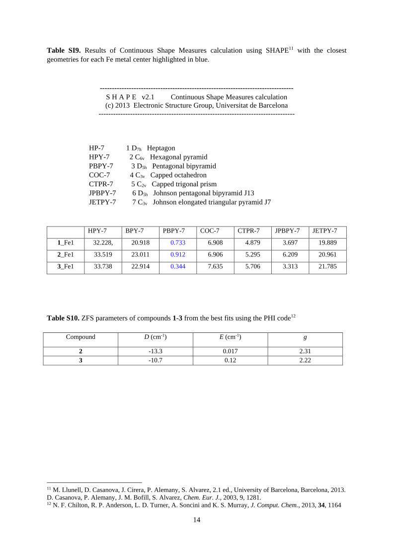
Table SI9. Results of Continuous Shape Measures calculation using SHAPE11 with the closest

geometries for each Fe metal center highlighted in blue.

--------------------------------------------------------------------------------

S H A P E v2.1 Continuous Shape Measures calculation

(c) 2013 Electronic Structure Group, Universitat de Barcelona

---------------------------------------------------------------------------------

HP-7 1 D7h Heptagon

HPY-7 2 C6v Hexagonal pyramid

PBPY-7 3 D5h Pentagonal bipyramid

COC-7 4 C3v Capped octahedron

CTPR-7 5 C2v Capped trigonal prism

JPBPY-7 6 D5h Johnson pentagonal bipyramid J13

JETPY-7 7 C3v Johnson elongated triangular pyramid J7

HPY-7 BPY-7 PBPY-7 COC-7 CTPR-7 JPBPY-7 JETPY-7

1_Fe1 32.228, 20.918 0.733 6.908 4.879 3.697 19.889

2_Fe1 33.519 23.011 0.912 6.906 5.295 6.209 20.961

3_Fe1 33.738 22.914 0.344 7.635 5.706 3.313 21.785

Table S10. ZFS parameters of compounds 1-3 from the best fits using the PHI code12

Compound D (cm-1) E (cm-1) g

2 -13.3 0.017 2.31

3 -10.7 0.12 2.22

11 M. Llunell, D. Casanova, J. Cirera, P. Alemany, S. Alvarez, 2.1 ed., University of Barcelona, Barcelona, 2013.

D. Casanova, P. Alemany, J. M. Bofill, S. Alvarez, Chem. Eur. J., 2003, 9, 1281. 12 N. F. Chilton, R. P. Anderson, L. D. Turner, A. Soncini and K. S. Murray, J. Comput. Chem., 2013, 34, 1164

15

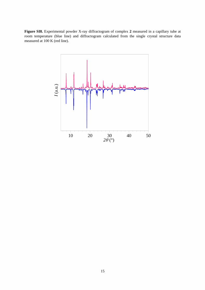
Figure SI8. Experimental powder X-ray diffractogram of complex 2 measured in a capillary tube at

room temperature (blue line) and diffractogram calculated from the single crystal structure data

measured at 100 K (red line).

10 20 30 40 50

[FeLH2N3O2Ph2

Ni(CN)4]n

I (a

.u.)

2 (°)

CIF

capillary

16

Figure SI9. Solid-state 57Fe Mössbauer spectra of 1─3 measured at 80 K shown with circle markers

along with the best spectral fits for a high spin FeII site for the parameters indicated in the text.

17

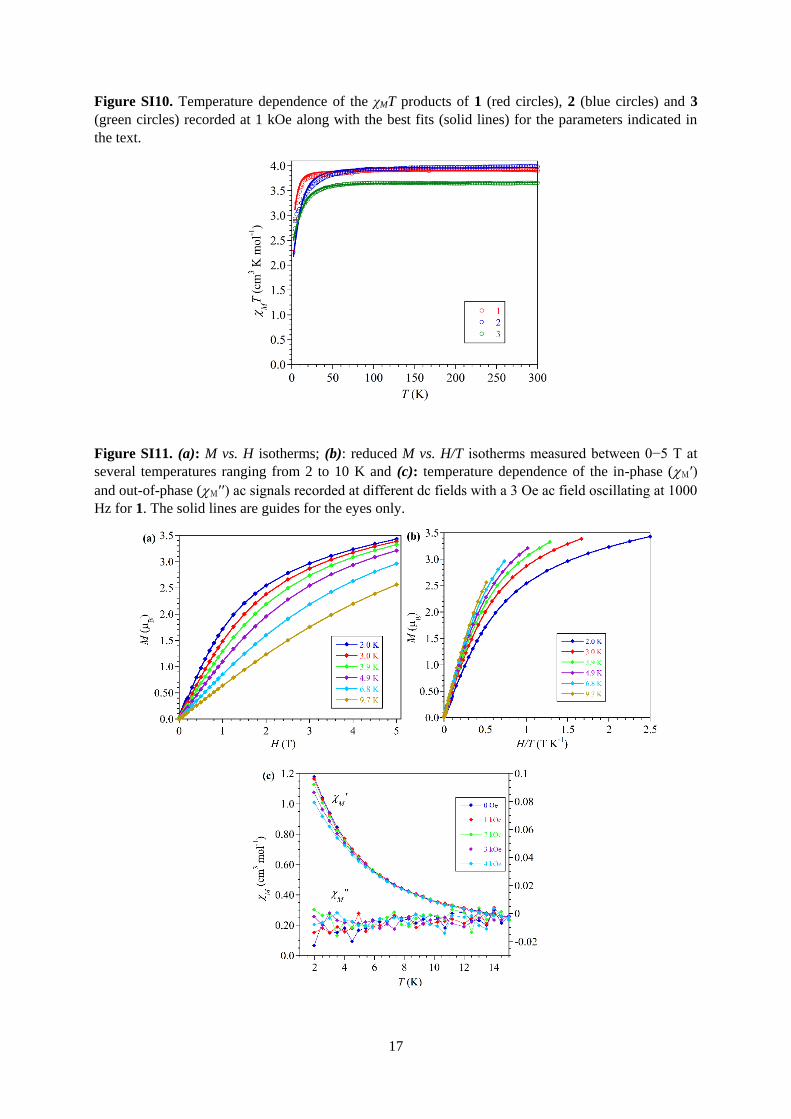
Figure SI10. Temperature dependence of the χMT products of 1 (red circles), 2 (blue circles) and 3

(green circles) recorded at 1 kOe along with the best fits (solid lines) for the parameters indicated in

the text.

Figure SI11. (a): M vs. H isotherms; (b): reduced M vs. H/T isotherms measured between 0−5 T at

several temperatures ranging from 2 to 10 K and (c): temperature dependence of the in-phase (Μ′)

and out-of-phase (Μ′′) ac signals recorded at different dc fields with a 3 Oe ac field oscillating at 1000

Hz for 1. The solid lines are guides for the eyes only.

18

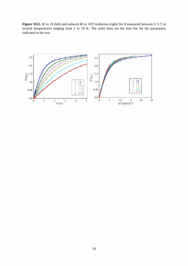
Figure SI12. M vs. H (left) and reduced M vs. H/T isotherms (right) for 2 measured between 0−5 T at

several temperatures ranging from 2 to 10 K. The solid lines are the best fits for the parameters

indicated in the text.

19

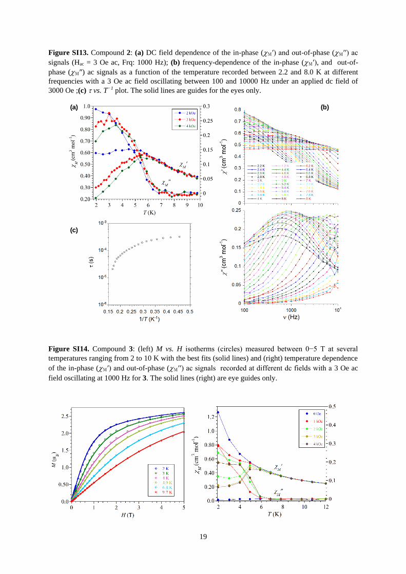
Figure SI13. Compound 2: (a) DC field dependence of the in-phase (Μ′) and out-of-phase (Μ′′) ac

signals (Hac = 3 Oe ac, Frq: 1000 Hz); (b) frequency-dependence of the in-phase (Μ′), and out-of-

phase (Μ″) ac signals as a function of the temperature recorded between 2.2 and 8.0 K at different

frequencies with a 3 Oe ac field oscillating between 100 and 10000 Hz under an applied dc field of

3000 Oe ;(c) vs. T−1 plot. The solid lines are guides for the eyes only.

Figure SI14. Compound 3: (left) M vs. H isotherms (circles) measured between 0−5 T at several

temperatures ranging from 2 to 10 K with the best fits (solid lines) and (right) temperature dependence

of the in-phase (Μ′) and out-of-phase (Μ′′) ac signals recorded at different dc fields with a 3 Oe ac

field oscillating at 1000 Hz for 3. The solid lines (right) are eye guides only.

(a) (b)

(c)

20

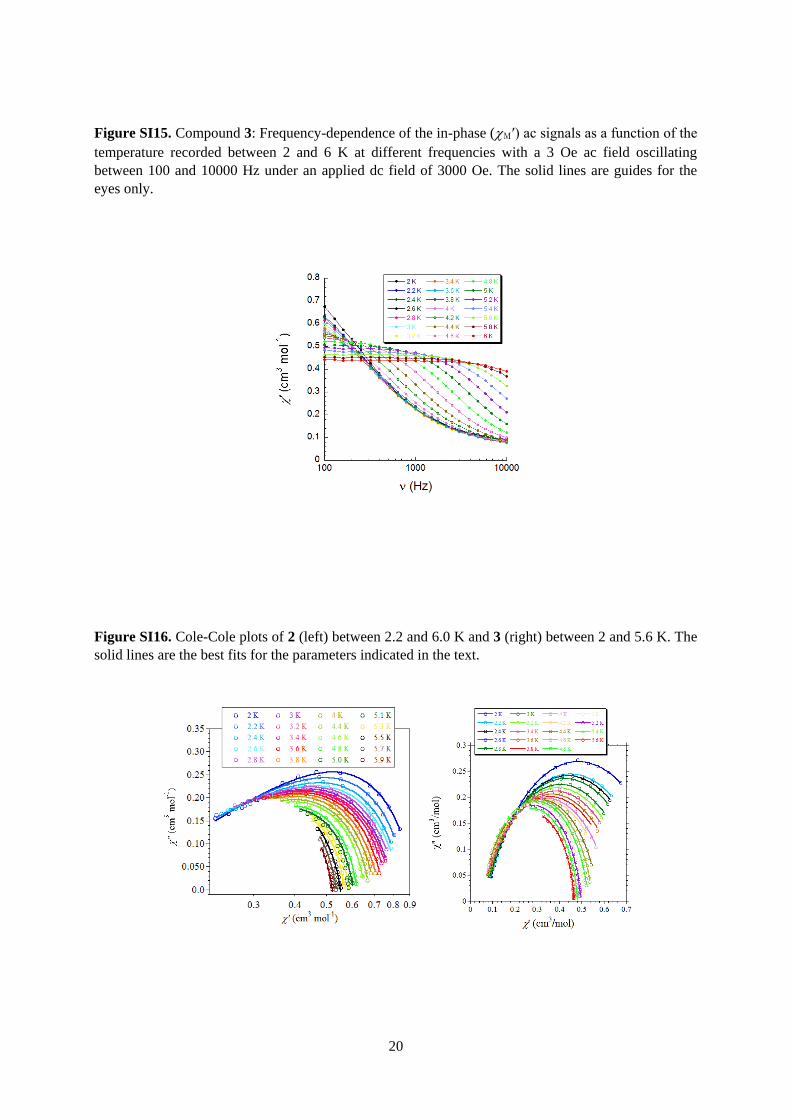
Figure SI15. Compound 3: Frequency-dependence of the in-phase (Μ′) ac signals as a function of the

temperature recorded between 2 and 6 K at different frequencies with a 3 Oe ac field oscillating

between 100 and 10000 Hz under an applied dc field of 3000 Oe. The solid lines are guides for the

eyes only.

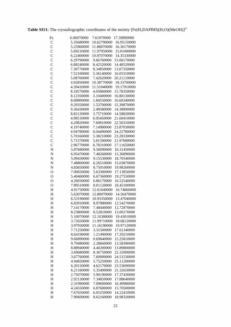
Figure SI16. Cole-Cole plots of 2 (left) between 2.2 and 6.0 K and 3 (right) between 2 and 5.6 K. The

solid lines are the best fits for the parameters indicated in the text.

21

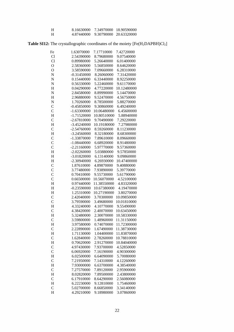
Table SI11: The crystallographic coordinates of the moiety [Fe(H2DAPBH)(H2O)(MeOH)]2+

Fe 6.06070000 7.61970000 17.39890000

C 5.35680000 10.62790000 16.95150000

C 5.25960000 11.86870000 16.30170000

C 5.69210000 11.97950000 15.01000000

C 6.22400000 10.87070000 14.35330000

C 6.29790000 9.66760000 15.06170000

C 6.88240000 8.42520000 14.48520000

C 7.30770000 8.34850000 13.07350000

C 7.52100000 5.36140000 16.05310000

C 5.08760000 7.42620000 20.21110000

C 4.92850000 10.38770000 18.33700000

C 4.39410000 11.51040000 19.17910000

C 8.18570000 4.05860000 15.78350000

C 8.12350000 3.10400000 16.80130000

C 8.68800000 1.84550000 16.60340000

C 9.29350000 1.53700000 15.39870000

C 9.36430000 2.48580000 14.38890000

C 8.82120000 3.75710000 14.58820000

C 4.98510000 6.95450000 21.60410000

C 4.20820000 7.60810000 22.56310000

C 4.19740000 7.14980000 23.87030000

C 4.94780000 6.04490000 24.22780000

C 5.70160000 5.38210000 23.28330000

C 5.71570000 5.81590000 21.97680000

C 2.96770000 6.78310000 17.11650000

N 5.87680000 9.56090000 16.31450000

N 6.95470000 7.48260000 15.36890000

N 5.09430000 9.15530000 18.70540000

N 7.48800000 6.26510000 15.03870000

N 4.83650000 8.75010000 19.98260000

O 7.00650000 5.63300000 17.13850000

O 5.40460000 6.67360000 19.27550000

O 4.26030000 6.86170000 16.52540000

O 7.89510000 8.01120000 18.45100000

H 4.91750000 12.61040000 16.74860000

H 5.63070000 12.80070000 14.56470000

H 6.53190000 10.93350000 13.47040000

H 6.83910000 8.97880000 12.54270000

H 7.14170000 7.48440000 12.72870000

H 8.23800000 8.52810000 13.00170000

H 5.10070000 12.10380000 19.43010000

H 3.72650000 11.99710000 18.68120000

H 3.97930000 11.16190000 19.97120000

H 7.71250000 3.31500000 17.61340000

H 8.64190000 1.21490000 17.29210000

H 9.66890000 0.69840000 15.25810000

H 9.79480000 2.28660000 13.58390000

H 8.88940000 4.40200000 13.89800000

H 3.69680000 8.36750000 22.32900000

H 3.67760000 7.60000000 24.51530000

H 4.94820000 5.75250000 25.11200000

H 6.20120000 4.62170000 23.53690000

H 6.21160000 5.35400000 21.32650000

H 2.75070000 5.90190000 17.37430000

H 2.92130000 7.34850000 17.88640000

H 2.31990000 7.09600000 16.49980000

H 4.24550000 6.87600000 15.70500000

H 7.67650000 6.05250000 14.22410000

H 7.90600000 8.62160000 18.98320000

22

H 8.16630000 7.34970000 18.90590000

H 4.87440000 9.30790000 20.63320000

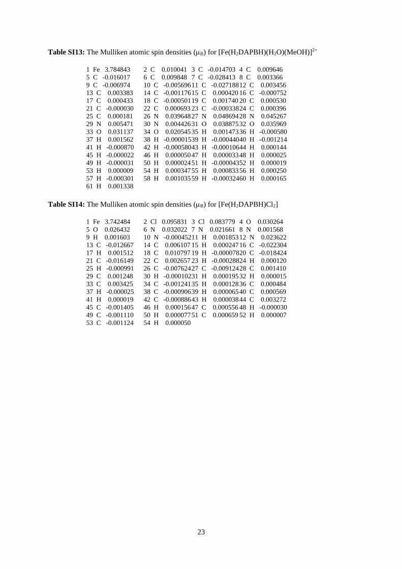
Table SI12: The crystallographic coordinates of the moiety [Fe(H2DAPBH)Cl2]

Fe 1.63070000 7.17710000 7.42720000

Cl 2.54390000 8.79680000 9.07540000

Cl 0.89980000 5.26640000 6.01400000

O 2.58360000 5.56850000 8.64620000

O 3.58590000 7.09660000 6.28310000

N -0.31450000 8.26060000 7.31420000

N 0.15440000 6.33440000 8.92250000

N 0.56330000 5.22460000 9.61170000

H 0.04290000 4.77220000 10.12480000

N 2.84580000 8.89990000 5.14470000

H 2.96880000 9.52470000 4.56750000

N 1.70260000 8.78500000 5.88270000

C -0.45850000 9.30860000 6.49240000

C -1.63300000 10.06480000 6.45600000

H -1.71520000 10.80510000 5.88940000

C -2.67810000 9.70490000 7.29220000

H -3.45240000 10.19180000 7.27980000

C -2.54760000 8.59260000 8.11230000

H -3.24560000 8.32180000 8.68300000

C -1.33870000 7.89610000 8.09660000

C -1.08440000 6.68920000 8.91480000

C -2.21160000 5.97770000 9.57360000

H -2.02260000 5.03880000 9.57850000

H -3.01820000 6.13140000 9.09860000

H -2.30940000 6.26930000 10.47400000

C 1.87610000 4.89870000 9.40880000

C 3.77480000 7.93890000 5.39770000

C 0.70410000 9.55730000 5.61790000

C 0.66500000 10.56070000 4.52100000

H 0.97440000 11.38550000 4.83320000

H -0.23590000 10.67380000 4.19470000

H 1.25310000 10.27190000 3.80270000

C 2.42040000 3.70300000 10.09850000

C 3.79590000 3.49680000 10.01810000

H 4.33240000 4.10770000 9.55490000

C 4.38420000 2.40070000 10.63450000

H 5.32480000 2.30070000 10.58330000

C 3.59800000 1.48960000 11.31150000

H 3.97580000 0.74070000 11.72300000

C 2.22890000 1.67490000 11.38730000

H 1.71130000 1.04400000 11.83870000

C 1.62840000 2.78260000 10.78810000

H 0.70620000 2.91270000 10.84040000

C 4.97430000 7.93700000 4.52850000

C 6.06920000 7.16190000 4.90300000

H 6.02500000 6.64090000 5.70080000

C 7.21950000 7.14310000 4.12260000

H 7.93000000 6.63700000 4.38540000

C 7.27570000 7.89120000 2.95900000

H 8.02820000 7.89500000 2.43800000

C 6.17910000 8.64290000 2.56080000

H 6.22230000 9.12810000 1.75460000

C 5.02700000 8.66850000 3.34140000

H 4.29210000 9.18980000 3.07860000

23

Table SI13: The Mulliken atomic spin densities (B) for [Fe(H2DAPBH)(H2O)(MeOH)]2+

1 Fe 3.784843 2 C 0.010041 3 C -0.014703 4 C 0.009646

5 C -0.016017 6 C 0.009848 7 C -0.028413 8 C 0.003366

9 C -0.006974 10 C -0.005696 11 C -0.027188 12 C 0.003456

13 C 0.003383 14 C -0.001176 15 C 0.000420 16 C -0.000752

17 C 0.000433 18 C -0.000501 19 C 0.001740 20 C 0.000530

21 C -0.000030 22 C 0.000693 23 C -0.000338 24 C 0.000396

25 C 0.000181 26 N 0.039648 27 N 0.048694 28 N 0.045267

29 N 0.005471 30 N 0.004426 31 O 0.038875 32 O 0.035969

33 O 0.031137 34 O 0.020545 35 H 0.001473 36 H -0.000580

37 H 0.001562 38 H -0.000015 39 H -0.000440 40 H -0.001214

41 H -0.000870 42 H -0.000580 43 H -0.000106 44 H 0.000144

45 H -0.000022 46 H 0.000050 47 H 0.000033 48 H 0.000025

49 H -0.000031 50 H 0.000024 51 H -0.000043 52 H 0.000019

53 H 0.000009 54 H 0.000347 55 H 0.000833 56 H 0.000250

57 H -0.000301 58 H 0.001035 59 H -0.000324 60 H 0.000165

61 H 0.001338

Table SI14: The Mulliken atomic spin densities (B) for [Fe(H2DAPBH)Cl2]

1 Fe 3.742484 2 Cl 0.095831 3 Cl 0.083779 4 O 0.030264

5 O 0.026432 6 N 0.032022 7 N 0.021661 8 N 0.001568

9 H 0.001603 10 N -0.000452 11 H 0.001853 12 N 0.023622

13 C -0.012667 14 C 0.006107 15 H 0.000247 16 C -0.022304

17 H 0.001512 18 C 0.010797 19 H -0.000078 20 C -0.018424

21 C -0.016149 22 C 0.002657 23 H -0.000288 24 H 0.000120

25 H -0.000991 26 C -0.007624 27 C -0.009124 28 C 0.001410

29 C 0.001248 30 H -0.000102 31 H 0.000195 32 H 0.000015

33 C 0.003425 34 C -0.001241 35 H 0.000128 36 C 0.000484

37 H -0.000025 38 C -0.000906 39 H 0.000065 40 C 0.000569

41 H 0.000019 42 C -0.000886 43 H 0.000038 44 C 0.003272

45 C -0.001405 46 H 0.000156 47 C 0.000556 48 H -0.000030

49 C -0.001110 50 H 0.000077 51 C 0.000659 52 H 0.000007

53 C -0.001124 54 H 0.000050