Simulation of stopped diffusions

F.M. Buchmann

Research Report No. 2004-03April 2004

Seminar fur Angewandte MathematikEidgenossische Technische Hochschule

CH-8092 ZurichSwitzerland

Simulation of stopped diffusions

F.M. Buchmann

Seminar fur Angewandte MathematikEidgenossische Technische Hochschule

CH-8092 ZurichSwitzerland

Research Report No. 2004-03 April 2004

Abstract

In this work we study standard Euler updates for simulating stopped diffu-sions. As an immediate application we discuss the computation of first exittimes of diffusions from a domain. We focus on one dimensional situations andshow how the ideas for the simulation of killed diffusions can be adapted tothis problem. In particular, we give a fully implementable algorithm to com-pute the first exit time from an interval numerically. The Brownian motioncase is treated in detail and extensions to general diffusions are given.Special emphasis is given to numerical experiments: For every ansatz, we in-clude numerical experiments confirming the conjectured accuracy of our meth-ods. Our algorithm is of weak order one in a weak sense. Comparisons withother algorithms are shown. Results that are superior to those obtained withother methods are presented. When approximating a first hitting time distri-bution the results obtained with our algorithm are much better than thoseachieved with other methods.

2

1 Introduction

1.1 Motivation

The simulation of a stopped diffusion with high accuracy is of significantinterest in many applications. Often, a good approximation of the first exittime of a stochastic process from a domain is needed to get good convergencein numerical simulation. A typical application is the probabilistic solution ofDirichlet problems in bounded domains. There, applying the Feynman-Kacformula to get a probabilistic representation of the solution, the first exittime plays a crucial role. Roughly speaking, a simulation procedure worksas follows: A path (a trajectory of a stochastic process) connected to thedifferential operator of the partial differential equation is simulated and oneintegrates along this path. The integration procedure has to be stopped whenthe path leaves the domain for the first time, and the boundary condition isevaluated at this first exit point. Approximating the mathematical expectationby a finite mean over a (large) sample then yields the (point-wise) Monte-Carloapproximation to the solution of the Dirichlet problem.We recall this formulation briefly and introduce some notation. Let D bea bounded domain in n-space with smooth boundary ∂D and consider thefollowing boundary value problem (BVP). For simplicity, we focus on Poisson’sequation:

1

24 u(x) + g(x) = 0, x ∈ D, u(x) = ψ(x), x ∈ ∂D. (1)

Consider the stochastic process

Xx(t) = x +∫ t

0dW (s), x ∈ D, (2)

where the integral is a stochastic integral in the sense of Ito and therefore(Xx(t))t≥0 is a Brownian motion starting at x [1,2]. We introduce the first exittime of (Xx(t))t≥0 from D:

τ(x) = inf{t > 0 : Xx(t) 6∈ D} = inf{t > 0 : Xx(t) ∈ ∂D}. (3)

The connection to the BVP (1) is given by the following version of the Feynman-Kac formula: The solution u(x) has the stochastic representation (under someregularity and smoothness conditions on g, ψ and D, see [3])

u(x) = E[ψ(Xx(τ(x))) +

∫ τ(x)

0g(Xx(s)) ds

]. (4)

Sometimes we find it more convenient to write u(x) = Ex[ψ(X(τ)) + f(τ)]where df = g(X(t)) dt with f(0) = 0. In this notation, the expectation is

1

taken with respect to the measure Px connected to the solution of dX = dWwith X(0) = x (and implicitly τ = τ(x)).

Clearly, the Feynman-Kac formulation (4) reveals its full strength in numer-ical simulations mainly (but not only) in high dimensions. Nevertheless, weconcentrate on one dimensional settings here, because: (i) the simple one di-mensional situation is already interesting in its own right and contains themain difficulties, and, (ii) we hope to be able to apply a big part of the ideaspresented here also in higher dimensions. If n becomes large, the domains Dare usually smooth with boundaries. Near to the boundary it looks flat. There,locally, the problem of a random walk approaching the boundary resemblesto some extent that of the one dimensional situation. However, for domainswith corners the situation becomes more complex – but this topic will not beaddressed here.

The algorithm we will construct exploits the fact that the stochastic differen-tial equations (SDEs) need only be approximated numerically in a weak sensewith a finite summation arithmetic mean approximating the expectation.

1.2 Difficulties in numerical simulation

At a first glance the numerical approximation of u(x) using (2,4) involves onlythe numerical solution of SDEs and averaging over a large sample (Monte-Carlo method [4]). This is nowadays a standard procedure in many applica-tions, see [5,6]. Nevertheless, if boundaries are involved, the situation is muchmore subtle.

The Euler scheme (or Euler-Maruyama scheme), due to its simplicity, is ofgreat interest. Applied to above situation with a fixed time step of size h, ittakes the form [5,6] X0 = x, f0 = 0 and

Xk+1 = Xk + ∆Wk and fk+1 = fk + g(Xk)h, for k = 0, 1, . . . . (5)

Here, an n-vector ∆Wk = W (tk+1)−W (tk) of i.i.d. normal random variableswith mean 0 and variance h (Gaussian random variables) is generated in eachtime step. We denote this distribution by the symbol N (0, h), ∆Wk ∼ N (0, h).The main difficulty presents itself: When should the (numerical) integration bestopped? In other words: How shall X(τ) and in particular τ be approximated?We shall concentrate on the approximation of τ in this article, correspondingto a constant boundary condition ψ in (1).

For a simple exposition of the main concepts, we consider D = (−∞, b) withx < b in what follows. The naive approach is to stop as soon as Xk ≥ b and totake as an approximation for the first hitting time of level b either τ ≈ (k−1)h,

2

τ ≈ kh or a certain value between these two values. The drawback of this ap-proach is the loss of accuracy: Although the Euler scheme is of weak order onefor a fixed final time T with M + 1 discretization points (giving h = T/M inour notation), the rate of convergence (even in the weak sense) in the pres-ence of a boundary reduces to O(

√h), i.e., it is of weak order one half [7]. The

use of exact Gaussian random variables for the increments of the Brownianmotion in (5) causes the following important drawback: The resulting discretetime random walk is no longer restricted to the closure of the domain underconsideration. In particular, (X(t))t≥0 (which we try to approximate) mightbecome larger than b within any temporal discretization subinterval: Althoughthe discrete random walk resulting from the Euler approximation (5) is exactin distribution sense, it gives the process values only at discrete tk = kh. Inbetween, for tk < t < tk+1, we have no information on the behaviour of thecontinuous process X(t) that we wish to approximate. It is well known [8,9,7]that in numerical simulation one has to take into account the fact that any-where near the boundary the process might have left D and come back withinstep h: Even if both Xk and Xk+1 < b, it is not unlikely that X(t) ≥ b for somet ∈ (tk, tk+1) – the process X(t) might follow an excursion within h, implyingτ < tk+1. Obviously, the trivial stopping procedure (stopping only if Xk ≥ b)will overestimate τ , as no intermediate excursions are monitored.

1.3 An exit probability approach for killed diffusions

To overcome this problem, instead of the unbounded increments ∆Wk ∼N (0; h), bounded approximations can be used [10,11], or a quantization ap-proach is adequate, see [12] and references therein.Nevertheless, applying the usual Euler scheme (with ∆Wk ∼ N (0, h)) canhave its advantages as well. To restore usual first order convergence (in theweak sense), a simple hitting test was introduced by various authors, see [8,9]and references therein. This test has to be performed after each time stepwith Xk+1 < b. It estimates the probability that an excursion occurred within(tk, tk+1) if both Xk, Xk+1 < b and leads to improved statistics.We summarize the principal idea of this approach for killed diffusions: Let afixed T <∞ be given and suppose that we are interested in the approximationof Ex[F (X(T ))1T<τ ] for some measurable F : Paths that reach level b up to(and including) time T are killed, that is, they do not contribute to the expec-tation. If we have, after an Euler step tk → tk+1 = tk + h < T , that Xk+1 ≥ bthen, obviously, τ < T and the corresponding path is killed. To take into ac-count a possible excursion across level b if Xk+1 < b one proceeds as follows:At the time the test is performed (after a step), Xk+1 is known. Therefore, thebridge process [13, p.67] pinned in time-space coordinates at (tk, Xk) and at(tk+1, Xk+1) has to be considered (and will be denoted by XXk,h,Xk+1

(s)). Tocheck for a possible excursion, an i.i.d. random number distributed uniformly

3

in (0, 1) (denoted by u ∼ U) is generated and the path is killed if

u ≤ P[

suptk≤s≤tk+1

XXk,h,Xk+1(s) ≥ b

]= e−

2h

(b−Xk)(b−Xk+1), u ∼ U . (6)

Gobet proved that first order weak convergence can be obtained for the Eu-ler scheme when applying this test for killed diffusions in the presence of aboundary [7], see also [14].

1.4 Outline

The purpose of this work is to modify these ideas to the case of stopped (ratherthan killed) diffusions. In this case, we try to approximate expectations of theform Ex[F (X(τ), τ)] (see (4)). Our interest is hence in the actual value ofτ rather than being satisfied by the assertion that (or if) τ < T for somepredefined (deterministic) T . In other words, one wants to know (again in astatistical sense) when the first exit time actually took place – in contrast toasking only if the exit did already occur. To accomplish this task, we constructin a first stage the density of τ of the bridge process under considerationand sample in a later stage a random number from it. We show how a newinterpretation of the exit probability of the bridge process (6) as a distributionleads to more accurate results (yet of the same order) for exactly the samecomputational cost. We then further improve our algorithm for the case thata discrete Xk+1 falls outside D. In that case, clearly τ ≤ tk+1. Nevertheless,we show how to find an approximation for τ ∈ (tk, tk+1].We start with the Brownian motion case in Section 2. The simplicity of thisprocess will allow us to present our ideas precisely without obscuring detailsof notation. We then extend these ideas to general autonomous diffusions inSection 3. We always consider the two possible cases after a step: (i) Xk+1 ∈ D(in Sections 2.1 and 3.1 respectively) and (ii) Xk+1 6∈ D (in Sections 2.2 and 3.2respectively). We show results from numerical experiments in Section 4 wherewe first discuss a statistical study comparing various algorithms (section 4.1)and later show results of some applications to the Feynman-Kac formulation(section 4.2). We conclude in Section 5.

2 The Brownian motion case

To simplify notation we write y = Xk and z = Xk+1. Recall that for a Brow-nian motion application of the Euler scheme with step size h > 0 means thatz = y + ξ with ξ ∼ N (0, h). In what follows we denote the correspondingBrownian bridge pinned at (tk, y) and at (tk + h, z) by Xy,h,z(s) and its law

4

by Py,h,z[·]. Additionally, τ denotes the first hitting time of level b.

2.1 Inside: y, z < b (test for an excursion)

Recalling (6) we find the distribution, F , of the first hitting time τ = τ(y)wrt. Brownian bridge measure for t > 0 as

F (t) ≡ Py,h,z[τ ≤ t] = e−2t(b−y)(b−z) . (7)

The idea is now to generate a random variable T1 with distribution (7). Tothis end, invert (7) [5, p.12],

T1 = −2(b− y)(b− z)log u

, u ∼ U . (8)

The path hit b between tk and tk + h if T1 ≤ h (in a statistical sense). Inthat case, b was hit for the first time at t = tk + T1 and we approximateτ ≈ (k − 1)h+ T1.The application to the approximation of f(τ) using (5) (for example) is nowstraightforward and we show it only for this variant of our algorithm:

f(τ)(5)≈ h

k−1∑

i=0

g(Xi) + T1g(Xk). (9)

In what follows we will not write down these approximations explicitly butonly show how to generate the last summand (i.e. its length of integration).

2.2 Outside: y < b ≤ z (compute first exit time)

We first construct the needed density. Using absolute continuity of the mea-sures Py and Py,h,z we have [13, p.67]

Py,h,z[τ ∈ dt] = p(h; y, z)−1p(h− t; b, z)Py[τ ∈ dt]

where p(t; x, y) denotes the Gaussian transition density: p(t; x, y) dy = Px[Wt ∈dy]. Inserting [13, (1.2.0.2),p.198] for Py[τ ∈ dt] gives with y < b

Py,h,z[τ ∈ dt] =b− y√

2πt3

√h

h− t exp

(− (z − b)2

2(h− t) +(z − y)2

2h− (b− y)2

2t

)dt

(10a)

5

and after some algebra

Py,h,z[τ ∈ dt] = (b− y)

√h

2πt3(h− t) exp

(−((b− y)h− t(z − y))2

2ht(h− t)

)dt.

(10b)

We remark that some simple manipulations in the exponent show that thisformula reduces for h = 1 and y = 0 to [15, formula (2.1), Lemma 3].

We now show how to sample from (10). To simplify notation, we set y = 0and h = 1. We say that a random variable X follows the inverse Gaussiandistribution with parameters γ > 0, δ > 0 (and write X ∼ IG(γ, δ)) if it hasthe density [16]

P[X ∈ dx] =

√γ

2πx3exp

(−γ(x− δ)2

2δ2x

)dx, x > 0.

The basic observation is that if X ∼ IG(b2, b/(z − b)) then t = X/(1 + X) isa random variable with density (10) (with h = 1, y = 0).To see this, define p(t) for 0 < t < 1 as P0,1,z[τ ∈ dt] = p(t)10<t<1 dt (see(10)). By the substitution x = t/(1− t) ≥ 0 with dt = dx/(1 + x)2 we find

p(t) dt =b√2π

(1 + x)2

x√x

exp

(−(b− xz/(1 + x))2

2x/(1 + x)2

)dx

(1 + x)2

=b√

2πx3e−

b2

2x(1− z−bbx)

2

dx.

The claim now follows immediately with γ = b2 and δ = b/(z − b).For the general bridge, we find analogously that if X ∼ IG((b − y)2/h, (b −y)/(z−b)), then the random variable t = hX/(1+X) has density (10). Michaelet al. presented an algorithm to generate random variables Xs following theinverse Gaussian distribution [17, p.89].

In the case that z = Xk+1 > b we therefore generate X ∼ IG((b− y)2/h, (b−y)/(z − b)) using [17], set T2 = hX/(1 + X) and stop integration at tk + T2

(analogously to (9)).

3 Extension to general diffusions

We now expand the ideas presented for Brownian motion in Section 2 togeneral diffusions given by (compare with (2))

Xx(t) = x +∫ t

0µ(Xx(s)) ds+

∫ t

0σ(Xx(s)) dW (s), σ(·) > 0, (11)

6

i.e., Xx(t) solves the (autonomous) SDE dX = µ(X) dt + σ(X) dW withX(0) = x. The Euler approximation with step size h > 0 then reads (comparewith (5))

X0 = x and Xk+1 = Xk + µ(Xk)h+ σ(Xk)∆Wk, for k = 0, 1, . . . (12)

with corresponding continuous-time approximation (frozen coefficient approx-imation)

X(t) = Xk + µ(Xk)(t− tk) + σ(Xk)(W (t)−W (tk)), t ∈ [tk, tk+1).

To derive our formulae we therefore consider the constant coefficient diffusion

Xµ,σx (t) = x + µt+ σW (t), t > 0.

We further write Xµ,σy,h,z for the corresponding bridge pinned at y and z with

length h and denote its law by Pµ,σy,h,z.

Remark 1 In the context of approximating killed diffusions it was pointed outthat this frozen coefficient approximation gives incorrect asymptotics and thatmore sophisticated approximations should be used [18,19]. The application ofthese ideas to stopped diffusions remains a topic of ongoing research.

3.1 Inside (test for an excursion)

Consider the function f(u) = u/σ and define D(t) = f(Xµ,σx (t)). By Ito’s

formula [13,2], D satisfies dD = µ/σ dt+ dW with D(0) = x/σ, i.e. (D(t))t≥0

is a Brownian motion with drift ν = µ/σ (starting at x/σ), see [13, I.IV.5.and II.2.]. As before let τ be the first hitting time of level b > y. Obviously,

Pµ,σy,h,z [τ ≤ h] = P[(

sup0≤t≤h

Xµ,σy,h,z(t)

)≥ b

]= P

[(sup

0≤t≤hDf(y),h,f(z)(t)

)≥ f(b)

],

where Df(y),h,f(z) denotes the version of D which is pinned at f(y) and f(z)and has length h. Now (we set v = f(y), w = f(z) and c = f(b))

P[

sup0≤t≤h

Dv,h,w(t) ≥ c

]= Pv

[sup

0≤t≤hD(t) ≥ c;D(h) ∈ dw

]

=Pv[sup0≤t≤hD(t) ≥ c,D(h) ∈ dw

]

Pv [D(h) ∈ dw].

Inserting [13, (2.1.0.6),p.250 and (2.1.1.8), p.251] yields

Pµ,σy,h,z [τ ≤ t] = e−2tσ2 (b−z)(b−x), (13)

7

which is equivalent to [7, p.169]. Inverting (13) we get (compare with (8))

T1 = −2(b− y)(b− z)σ2 log u

, u ∼ U , (14)

where (we recall that) σ = σ(y).

3.2 Outside (compute first exit time)

For y < b < z we proceed similarly to Section 2.2. We have for 0 ≤ t < h thedensity [20, (3.7), p.371]

Pµ,σy,h,z[τ ∈ dt] =pµ,σ(h− t; b, z)pµ,σ(h; y, z)

Pµ,σy [τ ∈ dt] (15)

where pµ,σ(t; x, y) denotes the transition density of the solution to dX =µ dt+ σ dW . Solving Kolmogorov’s forward equation one finds

pµ,σ(t; x, y) =exp

(− (y−µt−x)2

2tσ2

)

√2πtσ2

.

To find the density of the first hitting time one solves for α > 0 the differentialequation [13, p.18]

[σ2

2

d2

dx2+ µ

d

dx− α

]u(x) = 0.

and combines the increasing and decreasing solutions (denoted by u↑ and u↓

respectively) to get the Laplace transform of τ

Eµ,σy[e−ατ

]=

u↑(y)/u↑(b), y ≤ b

u↓(y)/u↓(b), y ≥ b

= eµ

σ2 (b−y)−√µ2+2ασ2

σ2 |b−y| .

Inverting it (using [13, Appendix]) we get the density (recall that b > y)

Pµ,σy [τ ∈ dt] =b− y√2πt3σ2

e−(b−µt−y)2

2tσ2 dt.

Inserting everything into (15) yields

Pµ,σx,h,z [τ ∈ dt] =

b− y√2πσ2t3

√h

h− t exp

(− 1

2σ2

((z − b)2

(h− t) −(z − y)2

h+

(b− y)2

t

))dt.

Recalling (10) we thus generate X ∼ IG((b− y))2/(hσ2), (b− y)/(z− b)) andset T2 = hX/(1 +X) (where again σ = σ(y)).

8

4 Numerical experiments

We show results of extensive tests performed with the algorithm derived inthe previous Sections. For weak approximations, path wise convergence isnot required, but a good approximation of the distribution is important. Inour case, special emphasis is on the computation of first exit times. We thusstart (in Section 4.1) with a statistical test where we compare the numericallyobtained density of a simple first hitting time (i.e. a histogram) with theknown analytical density. We compare our algorithm with a variety of otherapproaches. At a later stage (in Section 4.2), we show the performance of ouralgorithm when applied to the numerical solution of some one dimensionalDirichlet problems via the stochastic representation of the solution.

4.1 Approximating the density of the first hitting time: a statistical compar-ison

We compute numerically the first hitting time (denoted by τ) of level b = 1of a Brownian motion. The corresponding density is

P0 [τ ∈ dt] =e−

12t√

2πt3dt, t > 0. (16)

It has its maximum at t = 13

where it forms a non-symmetrically shaped peak,and it has a very long tail. We performed two tests checking the approximationof the peak and of the tail respectively (peak test and tail test).

4.1.1 Setup

We briefly describe the precise setup for the statistical tests. As E0[τ ] = ∞and P0[τ ∈ dt] ≈ 0 for t ≈ 0 we compute a histogram only for t ∈ [T0, T1] with0 ≤ T0 < T1 <∞ fixed. If the size of the bins is very small, we choose T0 > 0such that every bin is hit with sufficiently high probability. If a simulatedpath ran longer than T1 it was stopped and thus contributes only to the tailof the corresponding histogram (which was not included into the χ2-test). Tomeasure the quality of the approximations we performed a χ2-test over twodifferent sets of (equidistant) time intervals (the bins of the histogram). As ameasure of approximation we computed [21]

χ2 =Nb−1∑

i=0

(Ni −Npi)2

Npi(17)

9

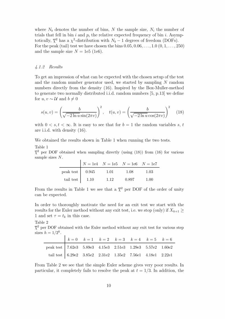
where Nb denotes the number of bins, N the sample size, Ni the number oftrials that fell in bin i and pi the relative expected frequency of bin i. Asymp-totically, χ2 has a χ2-distribution with Nb − 1 degrees of freedom (DOFs).For the peak (tail) test we have chosen the bins 0.05, 0.06, . . . , 1.0 (0, 1, . . . , 250)and the sample size N = 1e5 (1e6).

4.1.2 Results

To get an impression of what can be expected with the chosen setup of the testand the random number generator used, we started by sampling N randomnumbers directly from the density (16). Inspired by the Box-Muller-methodto generate two normally distributed i.i.d. random numbers [5, p.13] we definefor u, v ∼ U and b 6= 0

s(u, v) =

(b√

−2 ln u sin(2πv)

)2

, t(u, v) =

(b√

−2 ln u cos(2πv)

)2

(18)

with 0 < s, t < ∞. It is easy to see that for b = 1 the random variables s, tare i.i.d. with density (16).

We obtained the results shown in Table 1 when running the two tests.

Table 1χ2 per DOF obtained when sampling directly (using (18)) from (16) for varioussample sizes N .

N = 1e4 N = 1e5 N = 1e6 N = 1e7

peak test 0.945 1.01 1.08 1.03

tail test 1.10 1.12 0.897 1.00

From the results in Table 1 we see that a χ2 per DOF of the order of unitycan be expected.

In order to thoroughly motivate the need for an exit test we start with theresults for the Euler method without any exit test, i.e. we stop (only) if Xk+1 ≥1 and set τ = tk in this case.

Table 2χ2 per DOF obtained with the Euler method without any exit test for various stepsizes h = 1/2k.

k = 0 k = 1 k = 2 k = 3 k = 4 k = 5 k = 6

peak test 7.62e3 5.89e3 4.15e3 2.51e3 1.29e3 5.57e2 1.60e2

tail test 6.29e2 3.85e2 2.31e2 1.35e2 7.56e1 4.18e1 2.22e1

From Table 2 we see that the simple Euler scheme gives very poor results. Inparticular, it completely fails to resolve the peak at t = 1/3. In addition, the

10

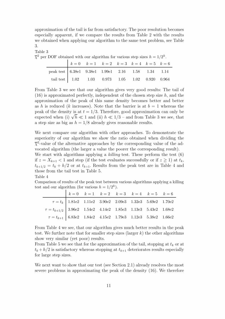
approximation of the tail is far from satisfactory. The poor resolution becomesespecially apparent, if we compare the results from Table 2 with the resultswe obtained when applying our algorithm to the same test problem, see Table3.

Table 3χ2 per DOF obtained with our algorithm for various step sizes h = 1/2k .

k = 0 k = 1 k = 2 k = 3 k = 4 k = 5 k = 6

peak test 6.38e1 9.38e1 1.99e1 2.16 1.58 1.34 1.14

tail test 1.02 1.03 0.973 1.05 1.02 0.920 0.964

From Table 3 we see that our algorithm gives very good results: The tail of(16) is approximated perfectly, independent of the chosen step size h, and theapproximation of the peak of this same density becomes better and betteras h is reduced (k increases). Note that the barrier is at b = 1 whereas thepeak of the density is at t = 1/3. Therefore, good approximation can only beexpected when (i)

√h� 1 and (ii) h� 1/3 – and from Table 3 we see, that

a step size as big as h = 1/8 already gives reasonable results.

We next compare our algorithm with other approaches. To demonstrate thesuperiority of our algorithm we show the ratio obtained when dividing theχ2-value of the alternative approaches by the corresponding value of the ad-vocated algorithm (the larger a value the poorer the corresponding result).We start with algorithms applying a killing test. These perform the test (6)if z = Xk+1 < 1 and stop (if the test evaluates successfully or if z ≥ 1) at tk,tk+1/2 = tk + h/2 or at tk+1. Results from the peak test are in Table 4 andthose from the tail test in Table 5.

Table 4Comparison of results of the peak test between various algorithms applying a killingtest and our algorithm (for various h = 1/2k).

k = 0 k = 1 k = 2 k = 3 k = 4 k = 5 k = 6

τ = tk 1.81e2 1.11e2 3.90e2 2.09e3 1.32e3 5.69e2 1.70e2

τ = tk+1/2 3.96e2 1.54e2 4.14e2 1.85e3 1.13e3 5.43e2 1.68e2

τ = tk+1 6.83e2 1.84e2 4.15e2 1.79e3 1.12e3 5.38e2 1.66e2

From Table 4 we see, that our algorithm gives much better results in the peaktest. We further note that for smaller step sizes (larger k) the other algorithmsshow very similar (yet poor) results.From Table 5 we see that for the approximation of the tail, stopping at tk or attk +h/2 is satisfactory whereas stopping at tk+1 deteriorates results especiallyfor large step sizes.

We next want to show that our test (see Section 2.1) already resolves the mostsevere problems in approximating the peak of the density (16). We therefore

11

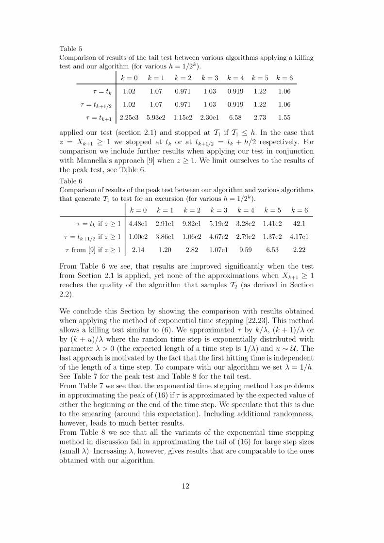
Table 5Comparison of results of the tail test between various algorithms applying a killingtest and our algorithm (for various h = 1/2k).

k = 0 k = 1 k = 2 k = 3 k = 4 k = 5 k = 6

τ = tk 1.02 1.07 0.971 1.03 0.919 1.22 1.06

τ = tk+1/2 1.02 1.07 0.971 1.03 0.919 1.22 1.06

τ = tk+1 2.25e3 5.93e2 1.15e2 2.30e1 6.58 2.73 1.55

applied our test (section 2.1) and stopped at T1 if T1 ≤ h. In the case thatz = Xk+1 ≥ 1 we stopped at tk or at tk+1/2 = tk + h/2 respectively. Forcomparison we include further results when applying our test in conjunctionwith Mannella’s approach [9] when z ≥ 1. We limit ourselves to the results ofthe peak test, see Table 6.

Table 6Comparison of results of the peak test between our algorithm and various algorithmsthat generate T1 to test for an excursion (for various h = 1/2k).

k = 0 k = 1 k = 2 k = 3 k = 4 k = 5 k = 6

τ = tk if z ≥ 1 4.48e1 2.91e1 9.82e1 5.19e2 3.28e2 1.41e2 42.1

τ = tk+1/2 if z ≥ 1 1.00e2 3.86e1 1.06e2 4.67e2 2.79e2 1.37e2 4.17e1

τ from [9] if z ≥ 1 2.14 1.20 2.82 1.07e1 9.59 6.53 2.22

From Table 6 we see, that results are improved significantly when the testfrom Section 2.1 is applied, yet none of the approximations when Xk+1 ≥ 1reaches the quality of the algorithm that samples T2 (as derived in Section2.2).

We conclude this Section by showing the comparison with results obtainedwhen applying the method of exponential time stepping [22,23]. This methodallows a killing test similar to (6). We approximated τ by k/λ, (k + 1)/λ orby (k + u)/λ where the random time step is exponentially distributed withparameter λ > 0 (the expected length of a time step is 1/λ) and u ∼ U . Thelast approach is motivated by the fact that the first hitting time is independentof the length of a time step. To compare with our algorithm we set λ = 1/h.See Table 7 for the peak test and Table 8 for the tail test.From Table 7 we see that the exponential time stepping method has problemsin approximating the peak of (16) if τ is approximated by the expected value ofeither the beginning or the end of the time step. We speculate that this is dueto the smearing (around this expectation). Including additional randomness,however, leads to much better results.From Table 8 we see that all the variants of the exponential time steppingmethod in discussion fail in approximating the tail of (16) for large step sizes(small λ). Increasing λ, however, gives results that are comparable to the onesobtained with our algorithm.

12

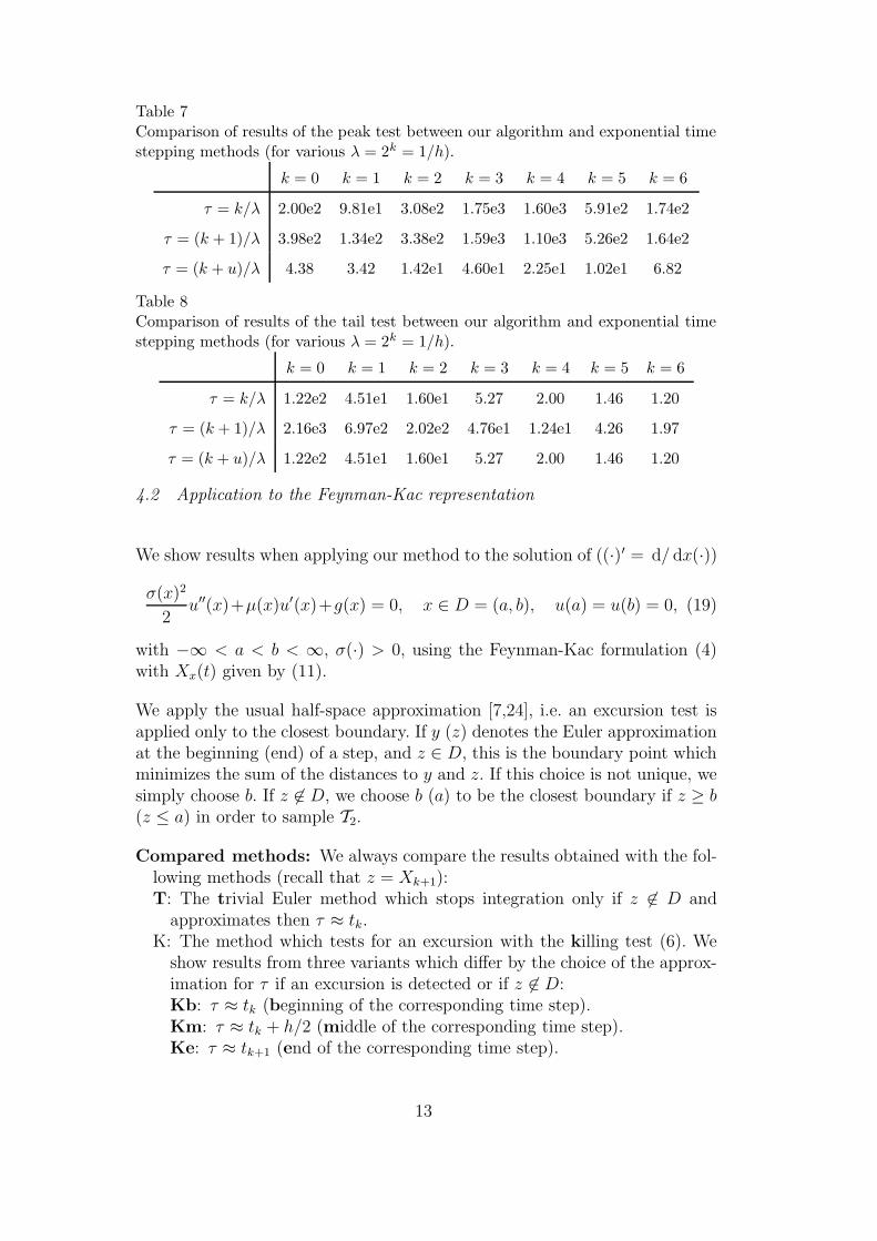
Table 7Comparison of results of the peak test between our algorithm and exponential timestepping methods (for various λ = 2k = 1/h).

k = 0 k = 1 k = 2 k = 3 k = 4 k = 5 k = 6

τ = k/λ 2.00e2 9.81e1 3.08e2 1.75e3 1.60e3 5.91e2 1.74e2

τ = (k + 1)/λ 3.98e2 1.34e2 3.38e2 1.59e3 1.10e3 5.26e2 1.64e2

τ = (k + u)/λ 4.38 3.42 1.42e1 4.60e1 2.25e1 1.02e1 6.82

Table 8Comparison of results of the tail test between our algorithm and exponential timestepping methods (for various λ = 2k = 1/h).

k = 0 k = 1 k = 2 k = 3 k = 4 k = 5 k = 6

τ = k/λ 1.22e2 4.51e1 1.60e1 5.27 2.00 1.46 1.20

τ = (k + 1)/λ 2.16e3 6.97e2 2.02e2 4.76e1 1.24e1 4.26 1.97

τ = (k + u)/λ 1.22e2 4.51e1 1.60e1 5.27 2.00 1.46 1.20

4.2 Application to the Feynman-Kac representation

We show results when applying our method to the solution of ((·)′ = d/ dx(·))

σ(x)2

2u′′(x)+µ(x)u′(x)+g(x) = 0, x ∈ D = (a, b), u(a) = u(b) = 0, (19)

with −∞ < a < b < ∞, σ(·) > 0, using the Feynman-Kac formulation (4)with Xx(t) given by (11).

We apply the usual half-space approximation [7,24], i.e. an excursion test isapplied only to the closest boundary. If y (z) denotes the Euler approximationat the beginning (end) of a step, and z ∈ D, this is the boundary point whichminimizes the sum of the distances to y and z. If this choice is not unique, wesimply choose b. If z 6∈ D, we choose b (a) to be the closest boundary if z ≥ b(z ≤ a) in order to sample T2.

Compared methods: We always compare the results obtained with the fol-lowing methods (recall that z = Xk+1):T: The trivial Euler method which stops integration only if z 6∈ D and

approximates then τ ≈ tk.K: The method which tests for an excursion with the killing test (6). We

show results from three variants which differ by the choice of the approx-imation for τ if an excursion is detected or if z 6∈ D:Kb: τ ≈ tk (beginning of the corresponding time step).Km: τ ≈ tk + h/2 (middle of the corresponding time step).Ke: τ ≈ tk+1 (end of the corresponding time step).

13

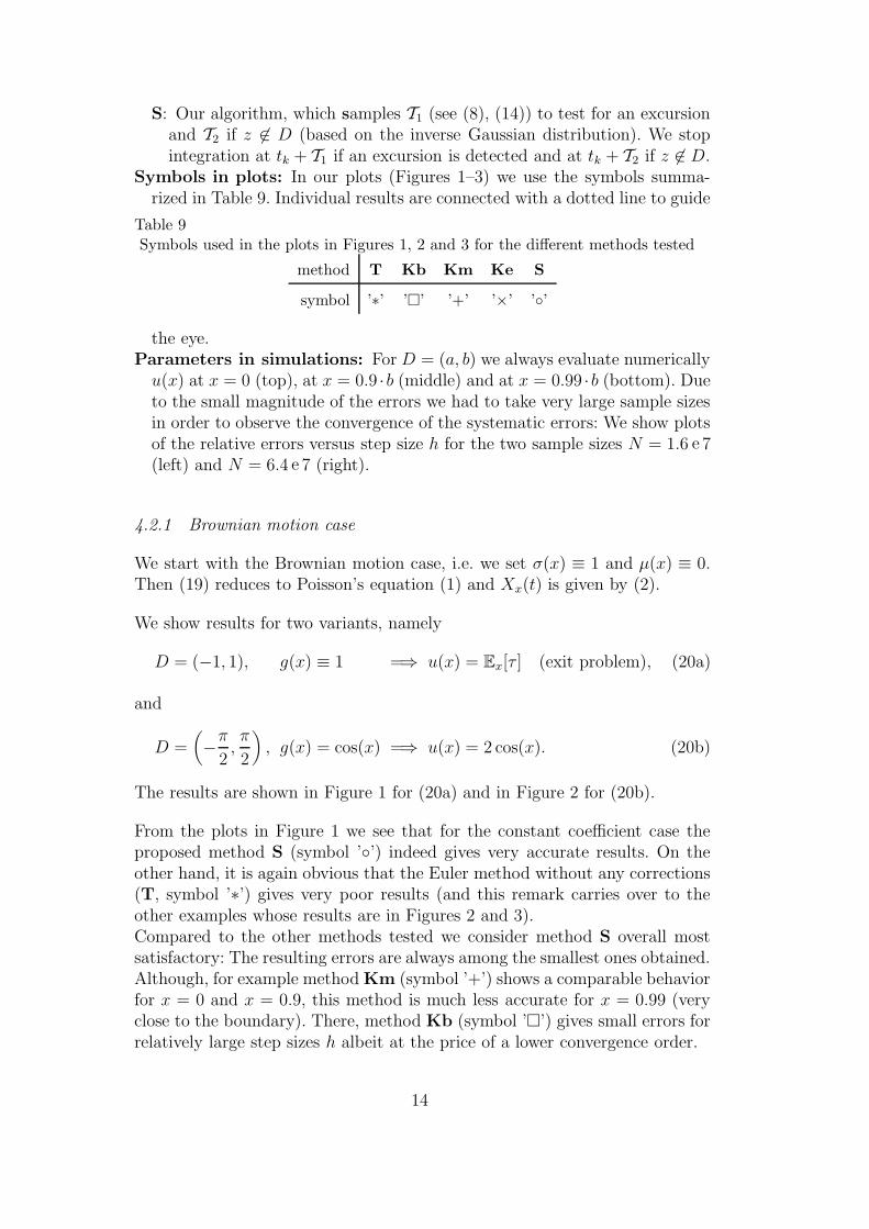
S: Our algorithm, which samples T1 (see (8), (14)) to test for an excursionand T2 if z 6∈ D (based on the inverse Gaussian distribution). We stopintegration at tk + T1 if an excursion is detected and at tk + T2 if z 6∈ D.

Symbols in plots: In our plots (Figures 1–3) we use the symbols summa-rized in Table 9. Individual results are connected with a dotted line to guide

Table 9Symbols used in the plots in Figures 1, 2 and 3 for the different methods tested

method T Kb Km Ke S

symbol ’∗’ ’�’ ’+’ ’×’ ’◦’

the eye.Parameters in simulations: For D = (a, b) we always evaluate numericallyu(x) at x = 0 (top), at x = 0.9 ·b (middle) and at x = 0.99 ·b (bottom). Dueto the small magnitude of the errors we had to take very large sample sizesin order to observe the convergence of the systematic errors: We show plotsof the relative errors versus step size h for the two sample sizes N = 1.6 e 7(left) and N = 6.4 e 7 (right).

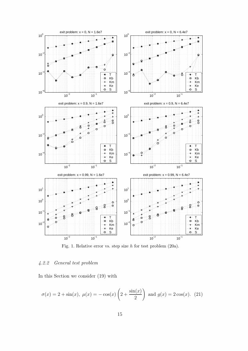
4.2.1 Brownian motion case

We start with the Brownian motion case, i.e. we set σ(x) ≡ 1 and µ(x) ≡ 0.Then (19) reduces to Poisson’s equation (1) and Xx(t) is given by (2).

We show results for two variants, namely

D = (−1, 1), g(x) ≡ 1 =⇒ u(x) = Ex[τ ] (exit problem), (20a)

and

D =(−π

2,π

2

), g(x) = cos(x) =⇒ u(x) = 2 cos(x). (20b)

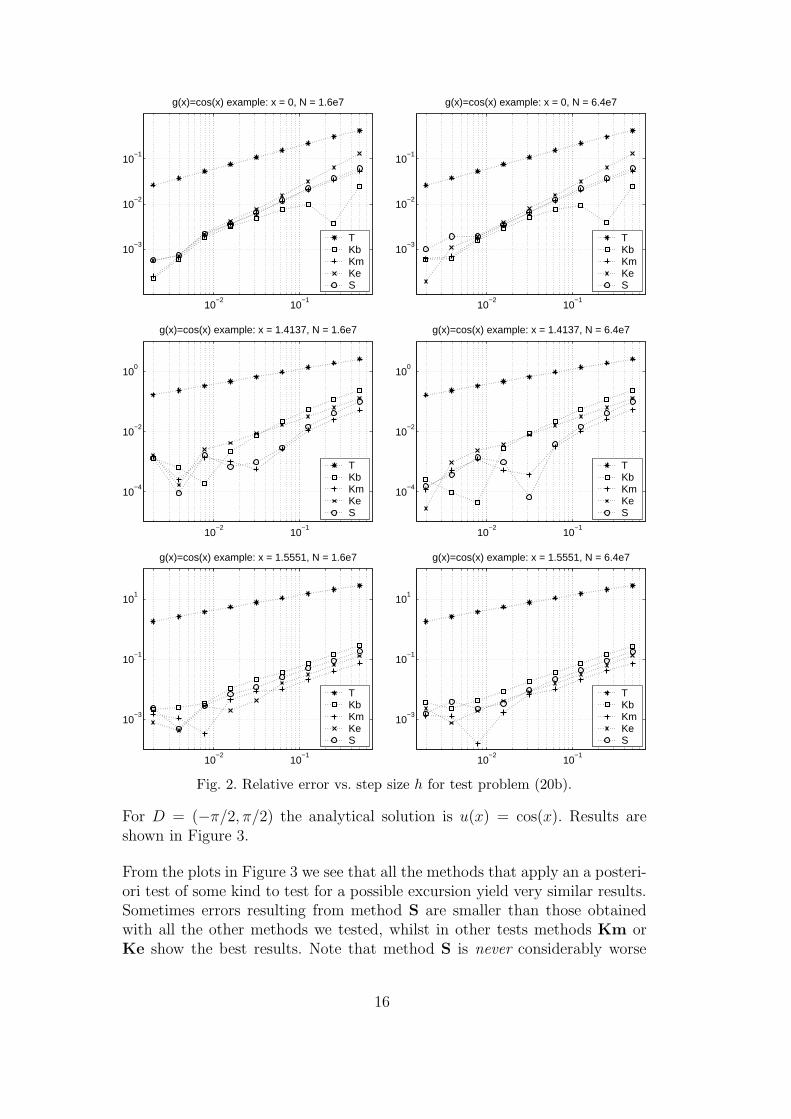
The results are shown in Figure 1 for (20a) and in Figure 2 for (20b).

From the plots in Figure 1 we see that for the constant coefficient case theproposed method S (symbol ’◦’) indeed gives very accurate results. On theother hand, it is again obvious that the Euler method without any corrections(T, symbol ’∗’) gives very poor results (and this remark carries over to theother examples whose results are in Figures 2 and 3).Compared to the other methods tested we consider method S overall mostsatisfactory: The resulting errors are always among the smallest ones obtained.Although, for example method Km (symbol ’+’) shows a comparable behaviorfor x = 0 and x = 0.9, this method is much less accurate for x = 0.99 (veryclose to the boundary). There, method Kb (symbol ’�’) gives small errors forrelatively large step sizes h albeit at the price of a lower convergence order.

14

10−2

10−1

10−6

10−4

10−2

100

exit problem: x = 0, N = 1.6e7

TKbKmKeS

10−2

10−1

10−6

10−4

10−2

100

exit problem: x = 0, N = 6.4e7

TKbKmKeS

10−2

10−1

10−4

10−2

100

exit problem: x = 0.9, N = 1.6e7

TKbKmKeS

10−2

10−1

10−4

10−2

100

exit problem: x = 0.9, N = 6.4e7

TKbKmKeS

10−2

10−1

10−2

10−1

100

101

exit problem: x = 0.99, N = 1.6e7

TKbKmKeS

10−2

10−1

10−2

10−1

100

101

exit problem: x = 0.99, N = 6.4e7

TKbKmKeS

Fig. 1. Relative error vs. step size h for test problem (20a).

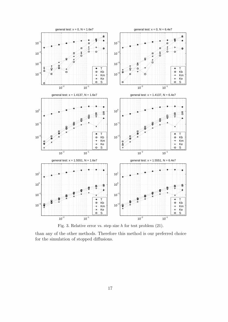
4.2.2 General test problem

In this Section we consider (19) with

σ(x) = 2 + sin(x), µ(x) = − cos(x)

(2 +

sin(x)

2

)and g(x) = 2 cos(x). (21)

15

10−2

10−1

10−3

10−2

10−1

g(x)=cos(x) example: x = 0, N = 1.6e7

TKbKmKeS

10−2

10−1

10−3

10−2

10−1

g(x)=cos(x) example: x = 0, N = 6.4e7

TKbKmKeS

10−2

10−1

10−4

10−2

100

g(x)=cos(x) example: x = 1.4137, N = 1.6e7

TKbKmKeS

10−2

10−1

10−4

10−2

100

g(x)=cos(x) example: x = 1.4137, N = 6.4e7

TKbKmKeS

10−2

10−1

10−3

10−1

101

g(x)=cos(x) example: x = 1.5551, N = 1.6e7

TKbKmKeS

10−2

10−1

10−3

10−1

101

g(x)=cos(x) example: x = 1.5551, N = 6.4e7

TKbKmKeS

Fig. 2. Relative error vs. step size h for test problem (20b).

For D = (−π/2, π/2) the analytical solution is u(x) = cos(x). Results areshown in Figure 3.

From the plots in Figure 3 we see that all the methods that apply an a posteri-ori test of some kind to test for a possible excursion yield very similar results.Sometimes errors resulting from method S are smaller than those obtainedwith all the other methods we tested, whilst in other tests methods Km orKe show the best results. Note that method S is never considerably worse

16

10−2

10−1

10−4

10−3

10−2

10−1

general test: x = 0, N = 1.6e7

TKbKmKeS

10−2

10−1

10−4

10−3

10−2

10−1

general test: x = 0, N = 6.4e7

TKbKmKeS

10−2

10−1

10−2

10−1

100

general test: x = 1.4137, N = 1.6e7

TKbKmKeS

10−2

10−1

10−2

10−1

100

general test: x = 1.4137, N = 6.4e7

TKbKmKeS

10−2

10−1

10−2

10−1

100

101

general test: x = 1.5551, N = 1.6e7

TKbKmKeS

10−2

10−1

10−2

10−1

100

101

general test: x = 1.5551, N = 6.4e7

TKbKmKeS

Fig. 3. Relative error vs. step size h for test problem (21).

than any of the other methods. Therefore this method is our preferred choicefor the simulation of stopped diffusions.

17

5 Summary

In this work, we presented an algorithm which leads itself to an efficient imple-mentation for the simulation of stopped diffusions. Our approach used stan-dard Euler updates and it was based on a method for the simulation of killeddiffusions. Instead of simply checking if a path has reached a certain levelwithin or at the end of a time step, we constructed a true stopping time tostop the integration. To achieve this goal, we sampled random numbers havingapproximatively the right distributions. In the case of diffusions with constantcoefficients, these distributions are by construction exact. This allowed us toadd a final Euler step of corresponding length to the simulated path and con-nected integrals. We think that this is the right approach for approximationsin the weak sense. Our numerical tests showed evidence that the resultingdistributions and thereof constructed weak approximations are of very highquality.

Acknowledgements

I would like to thank Wesley P. Petersen for continuous support throughout thepreparation of this paper. A special note of thanks goes to Alain-Sol Sznitmanfor providing me with reference [20] and explaining to me the details containedtherein.

References

[1] L. C. G. Rogers, D. Williams, Diffusions, Markov processes, and martingales.Vol. 1, Cambridge Mathematical Library, Cambridge University Press,Cambridge, 2000, Foundations, Reprint of the second (1994) edition.

[2] L. C. G. Rogers, D. Williams, Diffusions, Markov processes, and martingales.Vol. 2, Cambridge Mathematical Library, Cambridge University Press,Cambridge, 2000, Ito calculus, Reprint of the second (1994) edition.

[3] M. Freidlin, Functional integration and partial differential equations, Vol. 109of Annals of Mathematics Studies, Princeton University Press, Princeton, NJ,1985.

[4] N. Madras, Lectures on Monte Carlo methods, Vol. 16 of Fields InstituteMonographs, American Mathematical Society, Providence, RI, 2002.

[5] P. E. Kloeden, E. Platen, Numerical solution of stochastic differential equations,Vol. 23 of Applications of Mathematics (New York), Springer-Verlag, Berlin,1992.

18

[6] G. N. Milstein, Numerical integration of stochastic differential equations, Vol.313 of Mathematics and its Applications, Kluwer Academic Publishers Group,Dordrecht, 1995, translated and revised from the 1988 Russian original.

[7] E. Gobet, Weak approximation of killed diffusion using Euler schemes,Stochastic Process. Appl. 87 (2) (2000) 167–197.

[8] P. Baldi, Exact asymptotics for the probability of exit from a domain andapplications to simulation, Ann. Probab. 23 (4) (1995) 1644–1670.

[9] R. Mannella, Absorbing boundaries and optimal stopping in a stochasticdifferential equation, Phys. Lett. A 254 (5) (1999) 257–262.

[10] G. N. Milstein, M. V. Tretyakov, The simplest random walks for the Dirichletproblem, Teor. Veroyatnost. i Primenen. 47 (1) (2002) 39–58.

[11] F. Buchmann, W. Petersen, Solving Dirichlet problems numerically using theFeynman-Kac representation, BIT 43 (3) (2003) 519–540.

[12] G. N. Milstein, Weak approximation of a diffusion process in a bounded domain,Stochastics Stochastics Rep. 62 (1-2) (1997) 147–200.

[13] A. N. Borodin, P. Salminen, Handbook of Brownian motion—facts andformulae, 2nd Edition, Probability and its Applications, Birkhauser Verlag,Basel, 2002.

[14] E. Hausenblas, Monte Carlo simulation of killed diffusion, Monte Carlo MethodsAppl. 6 (4) (2000) 263–295.

[15] H. R. Lerche, D. Siegmund, Approximate exit probabilities for a Brownianbridge on a short time interval, and applications, Adv. in Appl. Probab. 21 (1)(1989) 1–19.

[16] J. L. Folks, R. S. Chhikara, The inverse Gaussian distribution and its statisticalapplication—a review, J. Roy. Statist. Soc. Ser. B 40 (3) (1978) 263–289, withdiscussion.

[17] J. R. Michael, W. R. Schucany, R. W. Haas, Generating random variates usingtransformations with multiple roots., Am. Stat. 30 (1976) 88–90.

[18] M. T. Giraudo, L. Sacerdote, An improved technique for the simulation of firstpassage times for diffusion processes, Comm. Statist. Simulation Comput. 28 (4)(1999) 1135–1163.

[19] P. Baldi, L. Caramellino, Asymptotics of hitting probabilities for general one-dimensional pinned diffusions, Ann. Appl. Probab. 12 (3) (2002) 1071–1095.

[20] A.-S. Sznitman, A limiting result for the structure of collisions between manyindependent diffusions, Probab. Theory Related Fields 81 (3) (1989) 353–381.

[21] M. G. Kendall, A. Stuart, The advanced theory of statistics. Vol. 2, 3rd Edition,Hafner Publishing Co., New York, 1973, inference and relationship.

19

[22] K. M. Jansons, G. D. Lythe, Efficient numerical solution of stochasticdifferential equations using exponential timestepping, J. Statist. Phys. 100 (5-6)(2000) 1097–1109.

[23] K. M. Jansons, G. D. Lythe, Exponential timestepping with boundary test forstochastic differential equations, SIAM J. Sci. Comput. 24 (5) (2003) 1809–1822(electronic).

[24] E. Gobet, Euler schemes and half-space approximation for the simulation ofdiffusion in a domain, ESAIM Probab. Statist. 5 (2001) 261–297 (electronic).

20