
Simulation of Sawmill Yields at Hyne Tuan Pine Mill
94
Faculty Health, Engineering & Sciences University of Southern QLD Simulation of Sawmill Yields at Hyne Tuan Pine Mill A dissertation submitted by Mr. Eyre Campbell In fulfilment of the requirements of ENG4112 Research Project Supervisor Kazem Ghabraie Submitted: October 23, 2013
Transcript of Simulation of Sawmill Yields at Hyne Tuan Pine Mill
Faculty Health, Engineering & Sciences
University of Southern QLD
Simulation of Sawmill Yields at Hyne Tuan Pine
Mill
A dissertation submitted by
Mr. Eyre Campbell
In fulfilment of the requirements of
ENG4112 Research Project
Supervisor
Kazem Ghabraie
Submitted: October 23, 2013

Abstract
Tuan plant processes between six and seven hundred thousand cubic meters of planta-
tion pine annually, on average this equates to around five thousand trees daily. Logs are
cut to length through a Log Merchandising machine. The numerical data generated by
the dimensional measuring system is proposed as feedstock for an ambitious computer
program that is designed to imitate the computerised, electrical and mechanical pro-
cesses of sawmill plant. Supposition being that a well fashioned predictive software can
provide an element of competitive advantage through the potential to aid production
planning. The program takes any user specified generic Tuan sawmill alpha-numeric cut
pattern code and interrogates into dimensional pattern cross-sections. The software has
been fashioned to select the sideboard width option that maximizes sawn volume yield
recovery.
The board trimming process synthesises laser vision sensing and computer processing to
determine the mechanical saw docking requirements; it is the vital final quality control
mechanism at the sawmill. Sensed wane dimensions of the timber are paired up against
programmed wane rules in the solutions computer to decide which trim saws will actu-
ate and dock to chip. The yield predictor program does a virtual trimmer processing of
every sawn board to assess the length output of sawn boards, dock to chip and sawdust
exhaust by saws.
The program is predicting the sawmill yields for sawn timbers, chip and sawdust, all the
yield indicators are reported as displayed outputs.
i

Limitations of Use
The Council of the University of Southern Queensland, its Faculty of Engineering and
Surveying, and the staff of the University of Southern Queensland, do not accept any
responsibility for the truth, accuracy or completeness of material contained within or
associated with this dissertation.
Persons using any or all of this material do so at their own risk, and not at the risk
of the Council of the University of Southern Queensland, its Faculty of Engineering and
Surveying or the staff of the University of Southern Queensland.
This dissertation reports an educational exercise and has no purpose or validity be-
yond this exercise. The sole purpose of the course pair entitled ‘Research Project’ is
to contribute to the overall education within the students chosen degree program. This
document, the associated hardware, software, drawings and other material set out in the
associated appendices should not be used for any other purpose: if they are so used it
is entirely at the risk of the user.
Prof Frank Bullen
Dean
Faculty of Engineering and Surveying
ii

Certification
I certify that the ideas, designs and experimental work, results, analyses and conclusions
set out in this dissertation are entirely my own effort, except where otherwise indicated
and acknowledged.
I further certify that the work is original and has not been previously submitted for
assessment in any other course or institution, except where specifically stated.
Mr. Eyre Jeffery Campbell
Student Number: W0039574
Signature Date
iii

Acknowledgments
Sincere thanks to Angela Pappin (Optimisation Engineer) for contributing to the tech-
nical understanding and interpretation of sawmill patterns and processes; a necessity for
true and accurate simulation.
To Gil Little (Senior Analyst/Programmer) for his contribution in enabling access to
stems and logs files as well as some ideas and strategies for potential integration of a
predictive modelling system with log-stocks.
Many thanks to Kazem Ghabraie (USQ Lecturer/Project Supervisor) for his support.
In the first instance for sharing the vision enough to have a transition from vision to
productive works and later for attention to MATLAB software code, LATEX, general
algorithm strategies and many tuning aspects related to quality of communication con-
text dissertation.
iv

Contents
Abstract i
Disclaimer ii
Certification iii
Acknowledgments iv
List Of Figures vi
List Of Tables x
1 Introduction and Background 1
1.1 Softwood Milling 2
1.2 Sawmill Simulation 6
1.3 Sawmill Sawing Simulation Literature Review 10
1.4 Risk Assessment 13
1.5 Resource Analysis 14
1.6 Project Time-lines 14
2 Log Break Down Process 16
2.1 Log Bucking System 16
2.2 Milling Pre-sorted Logs 22
3 Mining the Data Resource 26
3.1 Geometric Stem Data Retrieval and Router Processing 27
3.2 Data Bank for Stems and Logs 29
4 Mill Modelling 40
4.1 Decoding Sawmill Patterns 40
4.2 Sideboards 41
v

Contents
4.3 Transform Sawmill Pattern Code to Dimensions 41
4.4 Overlaying Cartesian Co-ordinates 43
4.5 Processing Face and Edge Wane 45
5 Trim Sawing Process 47
5.1 Trimmer Machine Centre 47
6 Virtual Product Volumation 56
6.1 F1 Sideboards 56
6.2 Cant Products 65
7 Performance of Simulation Software 68
7.1 Software Outputs 68
7.2 Accumulating Yields 70
7.3 Comparison of Software Yields and Actual Mill Yields 71
8 Summary of Findings and Future Direction 76
Bibliography 78
Appendices 80
Appendix A - Project Specification 81
October 23, 2013 vi

List of Figures
1.1 Hyne and Sons original hardwood milling operation in Maryborough Qld. 1
1.2 Tuan exotic pine plantation forest 3
1.3 Overview of Tuan softwood processing plant. 4
1.4 Trend in Australian housing starts and forecasts 5
1.5 Monthly change in total dwelling units approved (trend). 6
1.6 Total dwelling units approved (trend), Queensland. 6
1.7 Sawn timber from the Tuan sawmill. 7
1.8 Batch sorted log bays sitting in storage awaiting processing through the
sawmilling plant. 8
1.9 Chip and sawdust residue from the Tuan sawmill. 8
1.10 Black sections yield chip material and the yellow saw-lines yield dust 9
1.11 Logs tippled to the Sorting System. 10
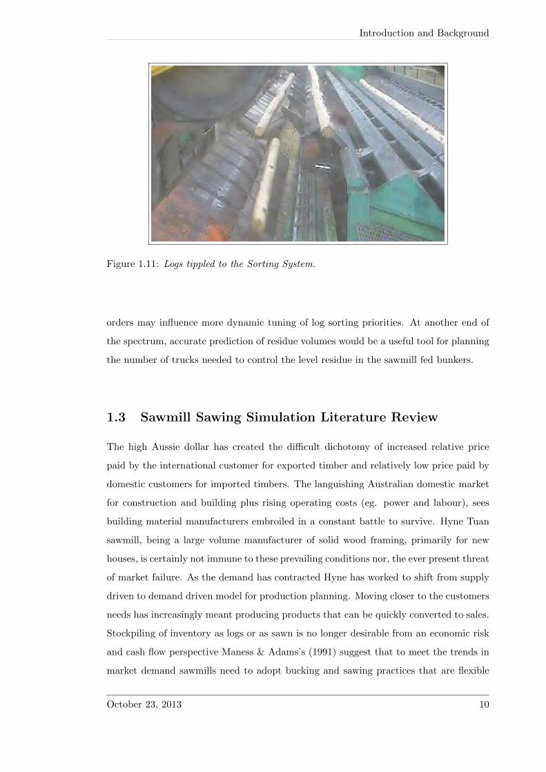
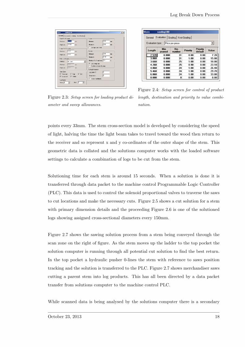
2.1 Stems (or trees) at approx. 19m length are input resource for the log merchandiser. 16
2.2 Overview of the log merchandiser system and process. 17
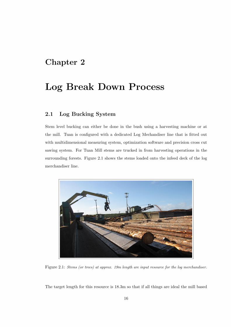
2.3 Setup screen for loading product diameter and sweep allowances. 18
2.4 Setup screen for control of product length, destination and priority to value
combination. 18
2.5 Log cut solution for a stem and stem dimensions. 19
2.6 Log 1 from the parent stem above showing bucket diameters every 150mm. 19
2.7 Parent stem processing into logs, from geometric scanning through to cutting. 19
2.8 Log sorting process is initiated when pneumatic cylinder driven tipples drop logs
in sequence to the sorter conveyor. 20
2.9 Showing the log sorting facilities, chain, kickers and bins. 21
2.10 Snapshot of Tuan virtual logstock program 22
vii

List of Figures
2.11 Virtual logstock data stored for each bin destination 23
2.12 Overview of the Tuan sawmill process and the flow direction of sawn products. 23
2.13 F1 & F2 Profiler unit and one of the internal heads. 24
2.14 Cut pattern with outside edges and kerfs dimensioned. 25
2.15 Chip removed for opening faces at first chipper canter. 25
2.16 After first rotation chip removed by second chipper canter. 25
2.17 After second rotation Profiler chips around the side boards. 25
2.18 Side boards sawn off producing sawdust. 25
2.19 After third rotation the cant is vertically sawn. 25
3.1 Hyne Model Perceptron Dimensional Measuring Instrument. 27
3.2 Side vision of a scanned log that has had scan points processed though a 6 in
data bucket router. 28
3.3 End view of a scanned log where data has been processed through 6 inch data
bucket router. 28
3.4 Extract from the logs file. 29
3.5 More complete version of logs file information. 30
3.6 Extract from a stems data file. 31
3.7 Mapping solutioned logs from a stem to the resource file. 32
3.8 Sourcing and loading the log profile from the stems file. 33
3.9 Simulator loop that controls the quantity of logs scanned for batch suit-
ability. 35
3.10 Locating the log in the parent stem. 36
3.11 General Program flowchart. 37
3.12 Program gathered log batch data for pre-selected bin. 39
4.1 Mapping a Tuan sawmill cut pattern code. 40
4.2 Cut pattern with F1 and F2 sideboards. 42
4.3 Cut pattern with F1 and F3 sideboards. 42
4.4 Dimensioned sawmill pattern. 42
4.5 Cant from pattern 3-3-2+c100-300. 42
4.6 Graphical depiction of the search options for increasing width of sideboards. 44
4.7 When sideboard edges are outside the bounds of the log then wane is introduced
along the outer face edges. 44
October 23, 2013 viii

List of Figures
4.8 Sideboard vertices and intersects with log perimeter co-ordinates. 44
4.9 Board wane diagram. 45
5.1 Block diagram of the trimming system. 48
5.2 Trimmer solution computers. 48
5.3 Operator controls material flow into trimming system. 49
5.4 Trimmer geometric scanning module. 50
5.5 Point lasers scanning a board as it moves through. 51
5.6 Trimmer scan head block diagram. 52
5.7 Scanned and solutioned boards entering the trim saws. 52
5.8 Trimmed boards exiting the trim saw booth. 52
5.9 Top view of a trim saw elements. 54
5.10 Isometric view of three trim saws. 54
6.1 Computed Percentage Edge and Face wane results for F1 sideboards on a bin
24 log. 57
6.2 Predicted length and volume recovery for all potential sideboard widths. 57
6.3 Extract from program code that checks that good section of 96mm wide F1
sideboard is longer than minimum standard length. 58
6.4 Extract of program code showing volumation of sideboard sections. 60
6.5 Face wane < 100% and Edge wane < 100%. 60
6.6 Face wane = 100% and Edge wane < 100%. 61
6.7 Face wane = 100% and Edge wane = 100%. 61
6.8 Face wane < 100% and Edge wane = 100%. 61
6.9 Summary yields for potential F1 sideboard widths. 62
6.10 Flowchart for volumating sawn board sections. 63
6.11 Area grouping for F1 sideboard when Face wane < 100% and Edge wane = 100% 64
6.12 Chord formed by the corners of the F1 sideboard. 65
6.13 Flowchart for volumating within wane specification sections of sideboard 66
6.14 Segmenting the right outer sideboard for computing area. 67
6.15 Cartesian co-ordinates are applied for geometric computation of outer cant board
area. 67
7.1 Log statistics 68
7.2 F1 sideboard yield indicators 69
October 23, 2013 ix

List of Figures
7.3 Cant board yield indicators 70
7.4 Accumulated sawmill yield indicators 71
7.5 Sawmill yield by log from simulator chart 72
7.6 Predicted sawn stock 73
7.7 Sawmill actual sawn recovery sample 73
7.8 Sawmill residues production monitor chart 74
7.9 Rate of Chip production vs. rate of Sawdust production 75
7.10 Profiler head 75
7.11 Addition of profiling saw segment kerfs from profiling units 75
October 23, 2013 x

List of Tables
1.1 Australia’s production of Sawn Timber plus selected Wood Products 4
3.1 Nominal and Actual target widths of sawn timber 38
3.2 Cut code for target thickness of sawn timber 38
3.3 Saw blade kerf 38
5.1 Trim saw table 54
xi

Chapter 1
Introduction and Background
Hyne and Sons quality milled timber brand and products have been around for more
than 120 years. During Hynes history there have been numerous boom and bust cycles
in the economies but the Hyne family business has manoeuvred for survival in economic
troughs, and then reinvigorated for expansion in the upswings. Originating in Queens-
lands Fraser Coast region Hyne began as a miller of native forest hardwoods. Figure 1.1
shows Hynes original hardwood mill situated on the banks of the Mary River along
which, logs were originally ferried from from selective harvesting operations on Fraser
Island.
Figure 1.1: Hyne and Sons original hardwood milling operation in Maryborough Qld.
Over the past 30 years Hyne has completely transitioned to milling only plantation
1

Introduction and Background
grown species of Pine. During the middle decade of this transition Hyne aspired to be
the number one softwood processor in Australia. Hyne now has three significant mills
dedicated to processing plantation pine. One is at Tuan (east of Maryborough) that
processes Exotic Pine varieties: Slash, Carribea , hybrids of the two and occasionally
native Hoop pine. The second operation is situated at Imbil (west of Gympie) is fully
focused on native Hoop pine and the third operation in Tumberrumba (west of Wagga)
is fully focused on exotic Radiata pine.
1.1 Softwood Milling
Softwood milling in many ways is vastly different to hardwood milling and to that extent
it is not so far fetched to classify them as different industries altogether. The softwood
industry operates from a base of large tracts of private and public plantations that have
been established and maintained primarily for the purpose of growing saw log and by
products. Figure 1.2 on the following page is a sample view of the Tuan plantation
forest that in total covers an area of 70 000 hectares, stretching from Maryborough in
the north right down to the northern fringes of Noosa in the south. Softwood mills can
be up to 20 times larger than hardwood mills generally because of the assured long term
availability of a resource that is fairly uniform.
Significant investment, foresight and hard work goes into the sustainable resource banks
that underpin softwood milling in this country. The rotation periods for the above men-
tioned species vary between 28 years to maturation for the exotics and 40 years for the
native hoop. In the meantime between harvesting these forests provide abundant eco-
logical habitats to a range of wildlife.
1.1.1 Securing a Position in Softwoods
To be a major player in the softwood industry requires significant capital investment in
plant and technology. Hyne annually processes volumes in the vicinity of 1.3 million cu-
bic metres. Very generally speaking recovered sawn percentage is around 50%, Table 1.1
October 23, 2013 2

Introduction and Background
Figure 1.2: Tuan exotic pine plantation forest
is the most recent and most comprehensive statistics for the Australian production of
sawn timbers and wood products. The table gives a sense of Hynes relative share of the
Australian sawn softwood, and contribution to wood products feedstock due to produc-
tion of sawing by-products of chip and sawdust.
Hyne has geared mills with highly automated processes, incorporating various machine
vision instruments, customized software and precisely controlled electronic, pneumatic
and hydraulic systems in order to cope with the required productivity. Figure 1.3 is an
aerial view of the Tuan pine processing plant, the finished timber section towards the
front of this view, the log breakdown areas are all toward the middle-rear and plantation
forest surrounds the plant.
All this machinery and technology comes at significant financial burden which predomi-
nantly must be leveraged by the business through financial institutions. When markets
slide abruptly into negative growth territory as they did around 2008 the providers of
financial leverage became increasing weary and the businesses ability to repay debts di-
minished due to an equally abrupt change in demand.
October 23, 2013 3

Introduction and Background
Table 1.1: Australia’s production of Sawn Timber plus selected Wood Products
Commodity 2003-04 2004-05 2005-06 2006-07 2007-08
SAWN Australian-Grown Timber
Softwood/Pines ’000m3 3 415 3 456 3 821 4 012 4 263
Hardwood/Eucalypts ’000m3 1 253 1 231 1 211 1 152 1 109
Total ’000m3 4 668 4 687 5 032 5 163 5 371
Fibreboard ’000m3 795 794 798 680 710
Particle board ’000m3 1 048 944 1 002 933 957
Paper and paperboard products
(printing, household, industrial) ’000t 1 956 1 945 1 926 1 907 1 933
Source: Australian Bureau of Agricultural and Resource Economics (online)
Figure 1.3: Overview of Tuan softwood processing plant.
October 23, 2013 4

Introduction and Background
1.1.2 Impact of Market Forces
When the Australian domestic building market is buoyant and the Australian dollar is
below parity then generally the softwood mills primary concern for profit maximization
is to maximize sawn recovery. This is because the highest cost to the business is the log
resource and the highest return is from sawn yield. In this market scenario cut patterns
are often selected so as to maximize the sawn yield which, is the highest value yield
product. Stockpiling whether it be logs for the sawmill or finished packs of product in
the warehouses is rarely a concern because the turn over of inventory is so positive and
average sale price high.
When demand is weaker and the Australian dollar is above parity (as is the recent trend)
the average sale price for timber is forced down; currently down some 25%. Housing In-
dustry Association and Australian Bureau of Statistics modelling such as supplied in
Figure 1.4, Figure 1.5 and Figure 1.6, the summary is that 2013 is to be a year of con-
traction for Australian new house starts and perhaps modest growth forecast for 2014
and 2015. These levels of activity are historically low.
Figure 1.4: Trend in Australian housing starts and forecasts
ABS 8731.0 (2013)
October 23, 2013 5

Introduction and Background
Primary focus switches to trying to cut only products that can be converted to sales with
minimum storage period and costs. Stockpiling at any part of the process is undesirable
because it represents a cost and risk to the business because of the market conditions.
Hynes new mission for the business is to become the supplier of choice. Sensitivity and
dynamic response to economic opportunities driven by solid relationships with customers
underpin the new focus.
Figure 1.5: Monthly change in total dwelling
units approved (trend).
Figure 1.6: Total dwelling units approved
(trend), Queensland.
ABS 8731.0(2013)
1.2 Sawmill Simulation
Ertas & Jones’s (1996) elucidate the design process begins with an identified need that
can be satisfied by a product of engineering effort. Identification of this need for a custom
built sawmill simulator to suit the Tuan mould/model has grown through the authors
journey with the stem and log breakdown team at the plant. Better management of
wood flows within the wood supply chain has been a clear priority for the majority of
forest products companies over the last couple of years (Apthorp 2013). Technology
research and development designed for implementation into the operations to gain some
improvement is a cultural driver at the plants. There are notable accomplishments to
date that fuel a continuation.
Realising a fully functional sawmill simulation of yield software would rank as a tech-
nology development achievement for the company. The potential for such a system to
October 23, 2013 6

Introduction and Background
bring new knowledge to the organization is multifaceted from an analytical research
perspective and product planning/mix perspective. It is desirable to have the provision
to look at a piece of software and have it predict in real time what is likely to be the
sawn output for the mill based (example of sawn material is on display at Figure 1.7)
on sorted batches of logs sitting in storage at the log yard, see Figure 1.8. The plant
Merchandiser is a reliable source of geometric data characteristics of stems.
Sawlog simulation could be programmed to display volumes of fibre likely to be recov-
ered from log yard batches/classes. The implications of a sawmill forecasting facility
relate primarily to production planning efficiencies. There is no foreseeable moral or
ethical dilemma generated with either the development or end uses of this product. The
intended system would be linked into the current log stock program and act merely as
an informative aid for production planning. There is no intention for the predictive
modelling to be linked into the machine control processes. Energy efficiency is certainly
gaining momentum in the management priority stakes and as such there is scope to
broaden simulation modelling to predict energy consumption in the sawmilling process
for any batch of logs.
Figure 1.7: Sawn timber from the Tuan sawmill.
Under consideration is the breakdown section of the Pine Processing Plant i.e. the
Merchandiser and the Linck Profiling line. Although common in Europe this plant com-
bination is not known to be replicated anywhere else in Australia. Hence Tuan log
breakdown systems must be considered as unique in nature and so the software will
be sculpted to suit the intricacies of that plant. If there were a simulation process pre-
October 23, 2013 7

Introduction and Background
Figure 1.8: Batch sorted log bays sitting in storage awaiting processing through the
sawmilling plant.
sawmill then for any given schedule of cut patterns planners can forecast the comparative
volume of high value sawn products (e.g. framing, fencing/landscape), versus residue
fibre proportions, in the form of wood chip and sawdust which as shown in Figure 1.9
are conveyed to dedicated storage bunkers before being transporting on as feedstock for
other production.
Figure 1.9: Chip and sawdust residue from the Tuan sawmill.
A small percentage increase in recovery translates into a significant financial advantage
for the timber manufacturer. Sawn product even as valued out of the mill (i.e. not yet
October 23, 2013 8

Introduction and Background
seasoned or planed) returns a higher price on average ($200/cubic unit) than does chip
($40/cu) or sawdust ($20/cu). For this reasons sawn recovery is a significant factor in
sawmill financial viability and there is always a strong push to maximise sawn recovery.
Figure 1.10 is a brief demonstration of how each product of sawmill yield evolves.
Figure 1.10: Black sections yield chip material and the yellow saw-lines yield dust
This project will investigate the possibilities of developing a suitable strategy and try
to design and build a computer program that might be integrated into current systems.
Ultimately the program output is envisaged to be a tool that can aid the Optimization
Engineer and Production Managers to improve production decision making. For example
accurate forward forecasting of residue volumes would be a useful tool for planning the
number of trucks needed to control residue levels in the bunkers for any given production
schedule. The ultimate concept for simulation package is to build it up to be efficient
enough to process individual logs as they are cut out of a parent stem, see Figure 1.11.
A simulation package could be developed for the log breakdown section of the mill and
if eventually fine tuned it could be a useful tool for both production and sales planning
alike. This project aims to investigate the possibilities of developing a suitable computer
program that is a good fit for the intricacies of the Tuan log breakdown process i.e. Linck
profiling lines and trimmers. Ultimately the program might be used by the optimization
engineer and production managers to improve production decision making. For exam-
ple more accurate forecasting of batch cutting volume requirements to meet customer
October 23, 2013 9
Introduction and Background
Figure 1.11: Logs tippled to the Sorting System.
orders may influence more dynamic tuning of log sorting priorities. At another end of
the spectrum, accurate prediction of residue volumes would be a useful tool for planning
the number of trucks needed to control the level residue in the sawmill fed bunkers.
1.3 Sawmill Sawing Simulation Literature Review
The high Aussie dollar has created the difficult dichotomy of increased relative price
paid by the international customer for exported timber and relatively low price paid by
domestic customers for imported timbers. The languishing Australian domestic market
for construction and building plus rising operating costs (eg. power and labour), sees
building material manufacturers embroiled in a constant battle to survive. Hyne Tuan
sawmill, being a large volume manufacturer of solid wood framing, primarily for new
houses, is certainly not immune to these prevailing conditions nor, the ever present threat
of market failure. As the demand has contracted Hyne has worked to shift from supply
driven to demand driven model for production planning. Moving closer to the customers
needs has increasingly meant producing products that can be quickly converted to sales.
Stockpiling of inventory as logs or as sawn is no longer desirable from an economic risk
and cash flow perspective Maness & Adams’s (1991) suggest that to meet the trends in
market demand sawmills need to adopt bucking and sawing practices that are flexible
October 23, 2013 10

Introduction and Background
and responsive.
Todoroki’s (1990) work introduced AUTOSAW system for sawing simulation. With this
software simulation was performed on both individual logs and batches of logs. Batch
size was not a restriction. Flexibility also allowed simulations to run interactively or as
an automated process. In 1990 automated sessions required 8 to 16 seconds to process
each log. An interactive session provided graphic images of the log at each stage of
simulation and it was possible to interrupt at any stage.
Maness & Adams (1991) presented and demonstrated three models for production plan-
ning for a sample sawmill. One of these models was a cutting pattern optimizer for
simulating the sawing of a log. The goal of integrating the three models was to choose
a sawing policy for a given log class that maximized the value of the lumber produced.
Potential advantages of moving from conventional static optimization product values
to dynamic product values where investigated by Todoroki & Ronnqvist (2002). Using
AUTOSAW product values where updated regularly according to previous timber pro-
duction. Todoroki & Ronnqvist found that this strategy could reduce the production of
un-ordered timber which alleviates storage and stockpiling issues.
Again using AUTOSAW as a research tool Todoroki & Monserud’s (2004) studied the
effect sweep has on lumber recovery. Todoroki & Monserud propose that a real log is
unique in its form, with several independent sources of variation (e.g. sweep, diameter
and knots). Each log can be sawn into products only once. To overcome multitude of po-
tential variation in results the sample of 51 real logs were converted into digital formats
and then increasingly bent at 1 inch increments in the virtual environment. Through
simulation it was found that conversion losses due to increasing sweep were represented
by an exponential decay function.
Later Todoroki, Monserud & Parry (2007) used AUTOSAW simulator to investigate the
effect of log ovality on lumber yield. Through simulation of virtual logs at incremental
rotations of 5 degrees (i.e. 0 to 355) they tested a hypotheses borrowed from Asikainen
& Panhelainen’s (1970) who proposed that if oval logs are sawn correctly and cubic con-
tent is determined on the basis of the minimum diameter, the sawing yield of an oval
October 23, 2013 11

Introduction and Background
log is better than that of a round log of the same size. When sawing is carried out in
the wrong position the opposite applies.
Todoroki et al. found that the most probable orientation for obtaining increased lumber
yield from oval logs was if the first saw cut is parallel to the major axis. Maximum
lumber yield was significantly greater from oval logs than from round logs. In some
cases yield from oval logs is less than that from round logs if rotation is not optimum.
Usenius & Heikkila (2007) introduced WoodCIM software which is currently used in
advanced planning at many Finnish sawmills. WoodCim is a computer aided sawmill
planning and controlling software developed at the Technical Research centre of Finland.
WoodCIM can be linked into mill computer system and provide support for product and
material flow control. WoodCIM post installation outcomes are linked with increased
sales value of production compared to less sophisticated planning methods. The goal of
WoodCIM is to achieve best profitability for sawing periods. For example a one month
strategy can be derived through an optimization model based on linear programming.
This sawing model works to optimally combine log supply, sawing possibilities and sales.
Song & Usenius (2007) evaluated InnoSim, a sawing simulator that has been developed
in an incremental manner in a series of research projects over the years. The paper em-
phasizes the push for logs used in simulation to better represent real logs. Aside from the
external log characteristics of diameters, length, taper and sweep they suggest modelling
the internal defects generated by knots and resin. They suggest that a distribution of
lumber quality could be predicted in simulation if statistics are gathered through trial
sawing investigations.
Lyhykainen et al. (2009) did sawing simulation using WoodCIM to predict sawn yields
of lumber grades and byproducts for Scots pine (plantation raw material in Finland).
According to this collection of published works it is apparent that WoodCIM and AUTO-
SAW are two simulation packages that have been utilized extensively for valid industry
research as well as for sawmill planning. WoodCIM has origins in Scandinavia and AU-
TOSAW in Canada. Enquiries to associated parties in each of these countries suggests
October 23, 2013 12

Introduction and Background
high levels of protection and privacy on these software. The Canadian group in particular
indicated some strict rules regarding the AUTOSAW simulator because only Canadian
Timber groups have the permission to access. This could indicate that the Canadians
feel that the simulator is a valued resource for achieving some competitive advantages.
The Scandinavian group where more willing to communicate particularly in relation to
apparent abilities of their simulator. However when it came to the nuts and bolts of the
simulator software and/or potential provision of a demo version there was no response.
Of the two major simulators uncovered in this review there is little doubt that the
Scandinavian built system is likely to be the more commercial opportunity for a sawmill
operation. AUTOSAW on the other hand, seems to be much more associated with
research and study objectives in order to establish conventions of practice for efficient
sawmilling.
1.4 Risk Assessment
Softwood sawmills comprise an abundance of heavy machinery and mobile plant such as
trucks and forklifts. Entry to Tuan site is security restricted for several reasons least not
the obligation to ensure that anyone entering site is sufficiently insured and have proven
that they are aware of personal safety obligations. The two primary requirements for
passing through security to the the plant is completion of a comprehensive induction
and secondly ensuring one is in possession of adequate personal protective equipment,
including: ear protection, isolation tags, high visibility clothing and steel capped boots.
The induction will include compulsory completion of modules and assessment for Site
Isolation and Emergency Response.
Walkways around site are clearly marked with yellow paint and must be followed by all
pedestrians to avoid entering into forklift operation zones. Since this project is primar-
ily a software development venture there is no real necessity to interrogate the physical
machinery which negates a good deal of the hazards.
October 23, 2013 13

Introduction and Background
There is no foreseeable environmental effects arising out the main objectives of this
project. The plant is concerned with processing plantation grown pine which is a renew-
able natural resource. All yields from the sawmill are renewable fibres all with useful
secondary applications. Although the project seeks to enhance efficiency of yield conver-
sion the potential advantages generally relate financially because the carbon conversion
is fairly neutral. Perhaps there maybe some side effect where coal fire sourced electricity
is more efficiently used as an input to the production timber fibres.
1.5 Resource Analysis
A driving factor for selecting this project is a desire to steer away from potential to
be caught with ballooning costs or critical component failures. This does not suggest
that the technical demands of simulating a high speed, highly automated plant are to
be underestimated. Aside from sourcing critical technical information from machine
manuals or from other technical staff the project has not acted as a burden to plant
operation. Aside from plant technical information (gathered in the literature review,
company sources and USQ project supervisor) the significant resources used in develop-
ment are a laptop computer, backup memory facility, email access, MATLAB software,
Latex software and feedstock Excel data files sourced from IT services.
Extension work would necessitate batch trial comparisons of sawmill runs and software
predictions. Such trials would present increased burden to plant operation because the
process would likely generate delays in production.
1.6 Project Time-lines
There a few essential foundation requirements and numerous potential avenues for en-
hanced software development. Technical analysis of log form parameters and how these
relate to conventions for batch cutting in the sawmill is complicated. As such the devel-
opment strategy is to simplify where possible in order to build a framework that is ready
to be extended upon. The nature of this undertaking somewhat limits the time available
for the dedicated programming orientation needed to get an algorithm and outputs for
October 23, 2013 14

Introduction and Background
all log form parameters. Some 50% of budgeted time is gobbled up by the technical
presentation aspects of the project (including mastering Latex). The general order and
approximated contributed workloads are listed below.
1. Literature review and contacting international bodies(40hrs);
2. Detailed background, machine and process specifics (30hrs);
3. Source stems and logs data file, import into MATLAB and write code to perform
the necessary manipulations (20hrs);
4. Write MATLAB code for the conversion of a sawmill cut pattern into geometric
dimensions of the associated cross-sectional representation (50hrs);
5. Write code for a virtual F1 sideboard, that determines the relative goodness of
fit of the sideboard at log every bucket interval. This is done for all potential
sideboard widths and the width that returns the highest volume sawn yield is
selected. (80hrs)
6. Construct working code loops that for example find a matching batch log for
processing and filters out non-matches (40hrs)
7. Code that volumates each 150mm section of the cant after virtual processing
(30hrs)
8. Code that volumes each 150mm section of the F1 sideboard after virtual processing
(40hrs)
9. Face and edge wane computation for F1 sideboards and outer cant products (30hrs)
10. Develop outputs for a single processed log and also for accumulated batch of logs
(70hrs)
October 23, 2013 15
Chapter 2
Log Break Down Process
2.1 Log Bucking System
Stem level bucking can either be done in the bush using a harvesting machine or at
the mill. Tuan is configured with a dedicated Log Mechandiser line that is fitted out
with multidimensional measuring system, optimization software and precision cross cut
sawing system. For Tuan Mill stems are trucked in from harvesting operations in the
surrounding forests. Figure 2.1 shows the stems loaded onto the infeed deck of the log
merchandiser line.
Figure 2.1: Stems (or trees) at approx. 19m length are input resource for the log merchandiser.
The target length for this resource is 18.3m so that if all things are ideal the mill based
16

Log Break Down Process
bucking system can retrieve three six metre logs; 6.2m being the maximum length that
the sawmill process due to plant configuration. Some quantity of supplied stems in-
evitably come in under the desirable length due to smaller parent tree or error in the
processor length detection (as is the case for stems that come in longer). Figure 2.2
is a plan view of the Tuan merchandiser operation, it shows the flow of stems from
debarking infeed, through the scanning and cross-cut sawing system and then onto the
sorting line as logs. Mobile log handling machines pick sorted logs up out of the bins
and subsequently place logs in batch storage bays ready for sawmill processing.
Figure 2.2: Overview of the log merchandiser system and process.
The objective of bucking optimization at the stem level is to maximise the stem value
by selecting the combination of logs to cross-cut from a stem that maximises potential
revenue. To do this task anticipated market prices and operational constraints must be
balanced. This decision making process involves programming optimizer software (see
Figure 2.3 and Figure 2.4) to compute the highest value combination of log products.
Log product parameters such as small and large end diameter, sweep range (degree of
bendyness) and length are programmed into the optimizer along with a priority and
value combination.
When a stem passes through the scanning zone time of flight optical energy range sensing
along four quadrants is able to determine to within 1mm accuracy what is the diameter
of the stem. Operating at 60 HZ the system is able to collect some 90+ range sensed
October 23, 2013 17
Log Break Down Process
Figure 2.3: Setup screen for loading product di-
ameter and sweep allowances.
Figure 2.4: Setup screen for control of product
length, destination and priority to value combi-
nation.
points every 33mm. The stem cross-section model is developed by considering the speed
of light, halving the time the light beam takes to travel toward the wood then return to
the receiver and so represent x and y co-ordinates of the outer shape of the stem. This
geometric data is collated and the solutions computer works with the loaded software
settings to calculate a combination of logs to be cut from the stem.
Solutioning time for each stem is around 15 seconds. When a solution is done it is
transferred through data packet to the machine control Programmable Logic Controller
(PLC). This data is used to control the solenoid proportional valves to traverse the saws
to cut locations and make the necessary cuts. Figure 2.5 shows a cut solution for a stem
with primary dimension details and the proceeding Figure 2.6 is one of the solutioned
logs showing assigned cross-sectional diameters every 150mm.
Figure 2.7 shows the sawing solution process from a stem being conveyed through the
scan zone on the right of figure. As the stem moves up the ladder to the top pocket the
solution computer is running through all potential cut solution to find the best return.
In the top pocket a hydraulic pusher 0-lines the stem with reference to saws position
tracking and the solution is transferred to the PLC. Figure 2.7 shows merchandiser saws
cutting a parent stem into log products. This has all been directed by a data packet
transfer from solutions computer to the machine control PLC.
While scanned data is being analysed by the solutions computer there is a secondary
October 23, 2013 18

Log Break Down Process
Figure 2.5: Log cut solution for a stem and stem dimensions.
Figure 2.6: Log 1 from the parent stem above showing bucket diameters every 150mm.
Figure 2.7: Parent stem processing into logs, from geometric scanning through to cutting.
October 23, 2013 19

Log Break Down Process
process going on that is dedicated to storing geometric information about each stem,
often referred to as a royalty process. Comma Separated Values (CSV) files are written
for each forest compartment during real time processing. Each day the CSV files are
securely copied through File Transfer Protocol out of the merch solutions computer for
various business applications.
While the solutions computer moves on to solving for subsequent stems the PLC carries
the responsibility of precisely (± 1 cm) driving each log to it’s correct batch location,
otherwise called ‘bin destination’. Figure 2.8 shows the very beginning of a logs journey
along the sorting process. There are 49 bin destinations on the sorter line. As the con-
veyor chain drives through the logs down the line an encoder sends pulses back to the
PLC. These are transformed into a length of travel. In the PLC each log has a counter
tagged to it and a loaded command count associated with where the solutions computer
decided this log is to reside due to form characteristics. This information was also passed
to the PLC in the data packet transfer for the cut solution.
Figure 2.8: Log sorting process is initiated when pneumatic cylinder driven tipples drop logs in
sequence to the sorter conveyor.
When the two counts match the PLC activates a solenoid valve for the relevant hydraulic
bin kicker. The cylinder actuation rotates the steel kicker assembly about a central shaft
to push the log into a bin. The top section of chain is around 150m in length (return
section also 150m), log separation is about 60cm, so at any one time there is a great deal
October 23, 2013 20

Log Break Down Process
of simultaneous machine routines involved with sorting the logs. Figure 2.9 is a perspec-
tive of the log sorting and storage facilities on the outfeed end of the merchandiser. Any
orphaned logs go right to the end of the line and a presence sensor activates kicker 48.
These logs will either be manually by log yard mobile plant or re-processed through the
merchandiser.
Figure 2.9: Showing the log sorting facilities, chain, kickers and bins.
Log output data from the merch is fed into a computer program called ‘virtual log-
stock’. Figure 2.10 shows the virtual log yard program that is a real time account of
logs in the log yard. Additions to stock are made by the merch cutting stems into
logs and subtractions are made when logs are processed through the mill. The dis-
play of numbered squares in Figure 2.10, represents a plan view of the merch sorting
system, showing all the physical classes of logs that are controlled and sorted by the
merchandiser. There are 48 hydraulically powered kickers that actuate any time a log
matching the bins class characteristics is driven to that location by the main chain.
With a mouse click on a particular bin (in the Figure 2.11, bin 24 has been selected)
we see a detailed breakdown of the logs currently stored in that class. Log age, species,
length and grade breakdown are all fairly vital indicators for production management de-
cision making. Ultimately it is advantageous to integrate a recovery breakdown that has
been assessed on a log by log and bucket by bucket basis using mathematical algorithms.
October 23, 2013 21

Log Break Down Process
Figure 2.10: Snapshot of Tuan virtual logstock program
2.2 Milling Pre-sorted Logs
The Tuan sawmill is a sequential line of machines that chip, rotate, profile and saw the
log into boards. Figure 2.12 gives a plan view of the Tuan sawmill showing the flow of
logs from log infeed to board sorting. The sawline is a German designed installation
from a company named Linck. The entire process is designed for high-speed production
capability. Drive line speeds can be manually varied and the current high speed for
driving logs down the sawline is 180m/min.
Each machine is equipped with tooling to perform the task, for example knives and
segments for chipping and profiling actions (see Figure 2.13) and saws for cutting. New
tooling is installed after every shift. Sometimes tooling might fail mid-shift, for example
a set of saws might get damaged or a chipper segment might come lose.
Aside from changing the tooling there is virtually no manual handling required for pro-
cessing logs down the sawline. The Linck line is a fully automated machine that reduces
October 23, 2013 22

Log Break Down Process
Figure 2.11: Virtual logstock data stored for each bin destination
Figure 2.12: Overview of the Tuan sawmill process and the flow direction of sawn products.
October 23, 2013 23

Log Break Down Process
Figure 2.13: F1 & F2 Profiler unit and one of the internal heads.
October 23, 2013 24

Log Break Down Process
a log batch down to sawn boards with seemingly little effort. Figure 2.14 to Figure 2.19
is a sequence of diagrams showing the log cross-sectional view, to demonstrate the Tuan
profiling line working on a Bin 24 log.
Figure 2.14: Cut pattern with outside edges and
kerfs dimensioned.
Figure 2.15: Chip removed for opening
faces at first chipper canter.
Figure 2.16: After first rotation chip removed
by second chipper canter.
Figure 2.17: After second rotation Profiler
chips around the side boards.
Figure 2.18: Side boards sawn off producing
sawdust.
Figure 2.19: After third rotation the cant
is vertically sawn.
October 23, 2013 25

Chapter 3
Mining the Data Resource
With the proposal established to develop and apply a virtual sawmill cut regime, (based
on potential cut patterns for each log class), on logs immediately after they have been
produced at the merchandiser. Logs cut at the merchandiser will generally sit in storage
as stock waiting for batch processing commands from the green mill. It is proposed
that in the meantime before batch processing at the sawmill, the Optimization and Pro-
duction Management personnel will have at their disposal, the luxury of an accurate
output forecast of sawdust, chip and sawn volumes. In theory production planners will
be informed (to some level of accuracy) about green mill output for any batch of logs
prior to a batch being called for cutting. In effect virtual log yard stock will be enhanced
to include virtual sawn stock.
Simulation of written code could only begin by sourcing a resource file. The ‘Logs
and Stems file’ from the company Information Services Team has served as a resource
platform function for foundations development. The stems sheet importantly contains
the stem counter which, is reset every eight hours (every shift). It also has a row of
diameters written at 150mm increments. These have been written to file by a three
dimensional tri-cam laser scanner system as depicted in Figure 3.1 on the next page.
26

Mining the Data Resource
Figure 3.1: Hyne Model Perceptron Dimensional Measuring Instrument.
3.1 Geometric Stem Data Retrieval and Router Processing
Scan chain speed is 120m/min and the scan heads operate at 60 Hz which, equates
to one snapshot scan produced every 33.3mm of the length of a stem. A high speed
photocell ensures length error margins are significantly less than 30mm. In each ‘6’ in
scan bucket, there will accordingly be between 4 and 5 ‘snapshots’ of scan data. Each
snapshot retrieves something like 90-120 points per scanner head.
The geometric scanning software uses all the points scanned to draw a continuous line
of best fit (setup to use line of least squares error method). This line of best fit forms a
distorted circle (i.e. the line will travel through 360 degrees and close the circle). A total
of 64 diameters are measured across this circle by calculating the centre point (centroid
of the shape) then, drawing a vertical line and measuring its length, stepping around
clockwise by 2.8 degrees (180 deg / 64 diameters), drawing the diameter through the
October 23, 2013 27

Mining the Data Resource
centre and measure the line length.
Data points scanned within the 6 inch bucket router are pushed together and a line of
best fit is drawn through the points. From this irregular near-circular closed 2-d shape
the 64 diameters at even spacing around the 360 degrees are calculated and averaged to
form the bucket diameter. Figure 3.2 is a log xyz file viewed with looklog program from
the side of a log. Figure 3.3 shows the end viewpoint of a log. The figures show the
grouped 64 points sourced from all the individual scanned points in bucket range spaced
at 6 inch intervals, particularly evident in the side view of Figure 3.2.
Figure 3.2: Side vision of a scanned log that has had scan points processed though a 6 in data
bucket router.
Figure 3.3: End view of a scanned log where data has been processed
through 6 inch data bucket router.
October 23, 2013 28

Mining the Data Resource
3.2 Data Bank for Stems and Logs
The high frequency of diameter readings written to the stems file gives rise to an op-
portunity for micro-scale simulation analysis on the logs. Although the logs sheet does
not have the bucket information it does have a link to the stems via the parent stem
number that is written in each log row, clearly indicated by the highlighted column in
Figure 3.4. This parent stem number is used as a link to the stems sheet and the useful
micro scale geometric information. Each stem however likely gives birth to on average
three logs so there is a challenge in linking the log to its associated diameter buckets in
the stems sheet. Given the log length from the logs sheet the number of buckets can be
calculated (by dividing by 150mm). Last column on the second row of Figure 3.5 indi-
cates that there is also a column (labelled ‘LogPosition’) in the logs sheet that identifies
the log position in the stem starting from zero through to the highest log count in a stem.
Figure 3.4: Extract from the logs file.
One weakness of this log file data is that log diameters are given only for the Small
End Diameter(SED) and Large End Diameter (LED). For increased predictive mate-
rial recovery accuracy it would be very preferable to have and use bucket data. The
more descriptive and desirable bucket data is only recorded in the stems CSV file. Data
given in Figure 3.6 is an example extracted from a stems CSV file, note that only a
portion of bucket diameters have been provided from a calibration event. Centre diam-
eter is the Huber diameter (Hdia). The additional strength of referencing to the stem
CSV bucket data is that the dimensional measuring system is regularly calibrated and
trade measurement certified within tolerances of 1mm for diameters and 10mm on length.
There is a technical challenge to find some way to reference the log back to the stem
October 23, 2013 29

Mining the Data Resource
Figure 3.5: More complete version of logs file information.
from the CSV file to get the full bucket data, (refer to Figure 3.6) . Each log is
(most often) only a portion of a parent stem. The solution will be to develop an al-
gorithm that will both reference the parent stem and the matching range of bucket
data. The added advantage of referencing to the stem CSV bucket data is that the
Dimensional Measuring System is regularly calibrated and Trade Measurement Cer-
tified (applied tolerance standards of ± 1mm for diameter and ± 10mm on length.
Log zero is the last section of a stem to be measured due to the saws o-lining at the
last bucket measured by the scanners (refer to Figure 3.7). To get the correct diameter
buckets for log zero the program needs to go to the end of the parent stem. This end of
the stem is most often the largest end of the stem due to taper and it is conventional to
have the smaller end in the lead. Thus for log zero the program starts loading bucket
diameters from the end of stems’ buckets minus the number of buckets associated with
that logs’ length. For log one the program starts loading bucket diameters from the end
of the stems buckets minus the number of buckets for log zero and minus the number of
buckets for log one. The process of loading bucket data for a log in position one ceases
when reaching the beginning of log zeros’ diameter buckets. The process increments for
any other target logs parented by the same stem, Figure 3.8 is a flowchart example of
this bucket diameter loading process.
October 23, 2013 30

Mining the Data Resource
Figure 3.6: Extract from a stems data file.
October 23, 2013 31

Mining the Data Resource
Figure 3.7: Mapping solutioned logs from a stem to the resource file.
Wood in raw form as a log is mostly non uniform character. Each log will be unique on
the basis of combined physical characteristics including: sweep, taper, and diameters.
Early development work on a program to gather useful log data from a provisioned file
highlighted the need for data filtering. To begin with logs belonging to just one pre-
determined merchandised bin are to be searched for and returned. The idea is that this
bin number plus a relevant sawmill cut pattern code can be input and changed by a
user. These inputs will be taken up as global variables by the programs processes.
A global counter variable counts the number logs retrieved by the program. This counter
also offsets the row number for storing sequential log bucket data. Alternatively it would
be possible to have only one row for storing the log bucket data, perform the required
analysis, store those results then write over the single bucket data row with the next
retrieved log. One of the drawbacks of storing all found logs bucket data is that logs are
not all the same length hence zeros are written on the end of any logs shorter than the
longest length. For example the longest log cut by the bucking system will nominally be
a 6m log, having 40 buckets while a mid length log nominally 4.8m length will have 32
buckets. The 4.8m log having 8 zeros at the end of its bucket data storage row. Trailing
zeros are obviously ignored during the application of cut pattern analysis to log diameter
data.
October 23, 2013 32

Mining the Data Resource
Figure 3.8: Sourcing and loading the log profile from the stems file.
October 23, 2013 33

Mining the Data Resource
3.2.1 User Control for Log Batch Size
The program has been designed with an outer loop (a ‘For’ loop). This loop controls how
many rows are to be incrementally searched for matches from within the logs file. From
a user perspective in order to increase the number of rows searched for a designated
batch of logs (say bin 24 logs) it is simply a matter of increasing the range allocated to
this outer loop, as depicted by variable ‘k’ in Figure 3.9.
3.2.2 Loading Appropriate Log Data
Identifying the logs to capture is a matter of using an arrangement of ‘If’ statements.
The process, as depicted in Figure 3.10 is designed to scan the contents of current logs
bin number and compare to the pre-defined bin number. An ‘And’ statement is com-
bined with the ‘If filter’ and serves to ascertain the log position. It is assumed that
the maximum log count in any one stem would be no more than six. Therefore six ‘If’
statements exist to look for the combinational match of bin number and log position in
the stem. Figure 3.11 condenses this particular process and explains how this part of the
program fits into the overall structure. Figure 3.12 gives the Matlab log data summary
output for a retrieved batch of logs, the counter returns how many logs matching the
desired.
3.2.3 Cant Cross-sectional Target Products
To reveal these cross sectional dimensions code elements must be identified in particular
order and decoded to reveal metric identities. To start from the centre with the thickness
of the cant. The first character in a pattern code specifies the cant thickness, so this
particular code says that the cant is three inches thick.
3-3-2 + c100 -300
Cant thickness is going to be the same as the width of the boards cut from the cant
after vertical saws break the cant down. According to Table 3.1 the 3 inch thick cant
has a target thickness of 75.5mm actual and 75mm nominal.
October 23, 2013 34

Mining the Data Resource
Figure 3.9: Simulator loop that controls the quantity of logs scanned for batch suitability.
October 23, 2013 35

Mining the Data Resource
Figure 3.10: Locating the log in the parent stem.
October 23, 2013 36

Mining the Data Resource
Figure 3.11: General Program flowchart.
October 23, 2013 37

Mining the Data Resource
Table 3.1: Nominal and Actual target widths
of sawn timber
Nominal(in) Nominal(mm) Actual(mm)
3 75 75.5
4 100 96 1
6 150 150
6 150 160 2
8 200 200
1 For most product, but 100 for 100×75 and 100×15.
2 160×38 in side boards are nominally 150 wide due
to later resaw to 2 x (76× 38).
Table 3.2: Cut code for target thickness of sawn timber
Code Nominal(in) Nominal(mm) Actual(mm)
1 5/8 15 15.7
2 1 25 26.5 1
3 1.5 38 39.6
4 2 50 50.0
1 for most product, but 25.5 for 100× 25.
Table 3.3: Saw blade kerf
Saw Unit Kerf/cut (mm)
Sideboards:
Inner 5.4
Outer 4.8
Cant Breakdown 4.2
October 23, 2013 38

Mining the Data Resource
Figure 3.12: Program gathered log batch data for pre-selected bin.
The addition of the second alpha numeric character is to describe thickness (decoded
by Table 3.2) of some cant boards. In the standard pattern code the thickness of these
boards are known only by non coded convention.
3-3-2 + c100 -300
Programmable computation is made simpler with the addition of this character. This
character is included to explain the thickness of timber pieces either at the centre of the
cant or neighbouring the cant; depending on which of the two is not described by the
second section of pattern code. In the example code the second section of code describes
the ’centre (c)’ as being 100mm wide. The preceding two characters say there are two
pieces of timber to be cut at the thickness described by the introduced character i.e. two
pieces at 39.6mm thick. These pieces will be cut from either side of the cant on the cant
width plane.
3- 3-2+c100 -300
The three code characters in the middle (c100) say that there is a 100mm wide product
being cut in the centre of the cant.
3-3-2+c100-300
October 23, 2013 39

Chapter 4
Mill Modelling
4.1 Decoding Sawmill Patterns
Tuan sawmill cut patterns (see Figure 4.1) are an important determinant of the sawmill
yield process. It is critical to this project that the conversion process from any cut
code to an understanding of the geometric dimensions is precise and fully automated.
Matlab code has been written to perform the computation of perpendicular dimensions
of a user selected pattern. Since the logs are modelled as circular, orientation conven-
tion has been described based upon the thickness and width plane orientation of the cant.
Figure 4.1: Mapping a Tuan sawmill cut pattern code.
40

Mill Modelling
The last three characters in the cut code is the code dedicated for side board locations
and their respective thickness (decoded in Table 3.2). Sideboards are generally cut as
a pair with each partner piece always cut opposite sides of the cant.
4.2 Sideboards
4.2.1 F1 Sideboards
The first character in the sideboard range (3) details presence or absence, if the char-
acter is zero then there will be no such sideboard and thickness of F1 sideboard pair is
zero. If numeric character greater than zero is present F1’s are to be cut from above and
below the cant (on the cant thickness plane). The kerf between cant and these particular
sideboards is 5.4mm and for the pair there is 10.8mm (i.e. two saw cuts), refer to Table
3.3.
3-3-2 + c100 - 300
4.2.2 F2 and F3 Sideboards
The second character (‘2’ in Figure 4.2 ) indicates presence and thickness of a sideboard
pair, located outside the first pair but in the same plane. The kerf to cut each one of
these sideboards is 4.8mm, so 9.6mm for the pair. The third character (‘2’ in Figure 4.3)
indicates presence and thickness of a sideboard pair to be cut from the outsides of the
cant in the cant width plane. These sideboards are removed at the cant breakdown saws
hence the kerf is only 4.2mm and 8.4mm for the pair.
4.3 Transform Sawmill Pattern Code to Dimensions
In the enduring example of a sawmill cut pattern code there are only F1 sideboards which
position above and below the thickness plane of the cant. To get the full dimension in
this orientation of the pattern the requirement is to add total sideboard saw kerf and
October 23, 2013 41

Mill Modelling
Figure 4.2: Cut pattern with F1 and F2 side-
boards.
Figure 4.3: Cut pattern with F1 and F3 side-
boards.
thickness of both the cant and the sideboards. Kerf for the inner sideboards breakdown
saw is 5.4mm, so the total kerf thickness for the removal of two sideboards is 10.8mm.
Finally adding the thickness of the two sideboards, the kerf and the cant thickness gives
one planar dimension of 75.5 + 2*(39.6)+10.8 =165.5mm actual (difference compared
with cut pattern diagram dimension is that product dimensions have been rounded to
integers).
Figure 4.4: Dimensioned sawmill pat-
tern. Figure 4.5: Cant from pattern 3-3-2+c100-300.
October 23, 2013 42

Mill Modelling
Perpendicular to cant thickness plane is the cant width plane. This pattern dimension is
the total width of the cant; all cant products plus the cant breakdown saw kerf of 4.2mm
for every cut. For this particular cut pattern there are two cant breakdown cuts each
with kerf of 4.2mm yielding three cant products; two at 39.6mm thick (code characters
3 and 5) and one at 100mm thick (code characters 7-10). The dimension in cant width
plane is therefore: 100 + 2*(39.6) + 8.4 = 187.6mm actual.
3- 3-2+c100-300
The thickness of a designated sideboard is always held constant (as prescribed by the
pattern code) but the width can vary depending on: fit to an individual log, width
categories (Table 3.1) and programmable priority and value settings. See Figure 4.6 for
demonstration of a sample of some potential width of F1 side boards examined through
simulation. At this stage of the development strategy it is decided to have the software
designed specifically for targeting the highest potential sawn yield rather than to delve
into the variables of optimising sideboard width according to fluctuations in customer
demands.
For virtual simulation and decision making in regards to max sawn yield regime on the
sideboards the potential vertices of the sideboards need be compared to corresponding
adjacent points on the perimeter of the log, see Figure 4.8 on the following page.
4.4 Overlaying Cartesian Co-ordinates
An adoptive strategy involves overlaying a Cartesian [x,y] coordinate profile with the
origin at the centre of the log, [x] is along the cant width plane and [y] is along the
cant thickness plane, see Figure 4.8. Cant thickness and sideboard breakdown kerf have
been established which means the exact location of the inner sideboard face edge on [y]
axis is determinable. The thickness of the sideboard is locked, the outer face edge can
be determined in a similar manner. By increasing the width of the sideboard the only
coordinates that will be variable are in relation to [x]. If the radius of the log can be
October 23, 2013 43

Mill Modelling
Figure 4.6: Graphical depiction of the search
options for increasing width of sideboards.
Figure 4.7: When sideboard edges are outside
the bounds of the log then wane is introduced
along the outer face edges.
established and the [y] intersect with sideboard face edge is constant then the intersect
in terms of [x] is determinable.
Figure 4.8: Sideboard vertices and intersects with log perimeter co-ordinates.
By introducing [x] coordinates that match the array of sideboard width options (refer to
Table 3.1) a comparative computational analysis between the vertices of the sideboard
and intersects to the outer edge of the log is performed. The result of such analysis
determines two things. Firstly if the vertices of the sideboard are located within the
bounds of the log and secondly if a board corner is located outside the log then the rel-
ative percentage of wane along the width face is computed, Figure 4.7 illustrates wane
introduced when projected sideboard edges stretch out beyond the perimeter of the log,
October 23, 2013 44

Mill Modelling
also see see Figure 4.9. The percentage wane parameter is highly sought after for this
project because there are, specific wane tolerance ranges governing whether a piece of
timber will be accepted by downstream grading stations or alternatively docked/rejected
and converted into chip.
4.5 Processing Face and Edge Wane
There are two places or types of wane that must be predicted one on the width face
(face of sawn), and the other on the thickness face (edge of sawn), refer Figure 4.9. At
the profiling line product specific limits for both face and edge wane can be set inde-
pendently. Primary and secondary wane limits can also be set where, primary wane
is allowed full length and secondary is allowed for a percentage of length. Typical pri-
mary and secondary limits are 30% face× 30% edge× 100% length and 33%face× 35%
edge× 30% length.
Figure 4.9: Board wane diagram.
First a strategy for modelling face and edge wane is identified and demonstrated by
example. In terms of [x] any point on a circle quadrant - 0 to π/2 can be described by:
x2 = r2 − y2
If the sideboard vertices are assigned Cartesian co-ordinates [x1,y1] and [x1,y2] for the
lower and upper corners respectively. For example if the radius of the log is 105 mm
for pattern ‘3-3-2+c100-300’, the origin is at the centre of pattern and log, then [y1]
co-ordinate will be 0.5*(75.5) + 5.4 = 43.15 and [y2] is 82.75 (i.e. y1 + sideboard
thickness). The [x] axis intersects between the sideboard and the outside of the log can
October 23, 2013 45

Mill Modelling
then be solved by substituting the y values and the log radius into:
x2n = r2 − y2n
The solutions for which are:
x1 = 95.7 and x2 = 59.8
Mirroring the result about the [y] axis indicates the maximum available material a side-
board located within the y axis range. The maximum material width of the inner face
of the sideboard according to this method is 191.45mm. The outer face has less material
as it is further from the centre; leaving cross section of only 119.6mm. If the sideboard
vertices extend beyond these values then edges will not be cut square and will inherit
wane on both face and edge.
The largest standard sideboard width (Table 3.1) that will fit inside the inner face is
160mm (actual). Projecting this width up to the top face means going beyond the out-
side of the log since the max material width here is 119.6mm. The difference between
these two values is the absolute measure of wane on the top face (i.e. 160 - 119.6 =
40.4). The relative percentage of face wane computed is 40.4/160 *100 = 25.25% which,
is within the acceptable range.
In the instance of edge wane the intersection of the outside perimeter of the log and edge
of the board needs be determined. In terms of [y] any point on a circle quadrant - 0 to
π/2 can be described by:
y2n = r2 − x2n
hence:
y23 = r2 − x21
The result for y3 is 68mm. Difference between y3 and y2 is 14.75mm (82.75 - 68). The
relative percentage of edge wane computed is 14.75/39.6 *100 = 37.25%. This would
fail the typical wane rule test because edge wane percentage is too high.
October 23, 2013 46

Chapter 5
Trim Sawing Process
Board trimming is the final breakdown process for unseasoned sawn timber at the Tuan
sawmill. Where once the inspection and docking process may have been manually
performed by human operator/s, the shear rate of volume being supplied by the
profiling line demands an automated solution with equal capacity handling capability.
5.1 Trimmer Machine Centre
The trimmer machine center is a system that integrates several major components. A
computer system calculates the maximum value of recoverable timber and chips for
each piece of material processed. The system uses accurate scanning, PCs and
dedicated software packages. The system scans material and calculates board solutions.
A Programmable Logic Controller (PLC) controls the timing and movement of machine
centre equipment. The scanning system determines thickness, width and length for
each material piece. A solution is computed by using the current set parameters and
the scan data. The parameters can be edited and allows for customization.
The solutions PC:
• Calculates board solutions and controls saw movement/activation through the
PLC.
• Sends commands to other PCs.
• Requests data from other PCs.
47

Trim Sawing Process
Figure 5.1: Block diagram of the trimming system.
Figure 5.2: Trimmer solution computers.
October 23, 2013 48
Trim Sawing Process
• Sends and receives PLC data.
• Stores solution parameters.
The Solutions PC is the controlling PC for the system. It uses scanner data to
calculate board solutions and position data for each piece.
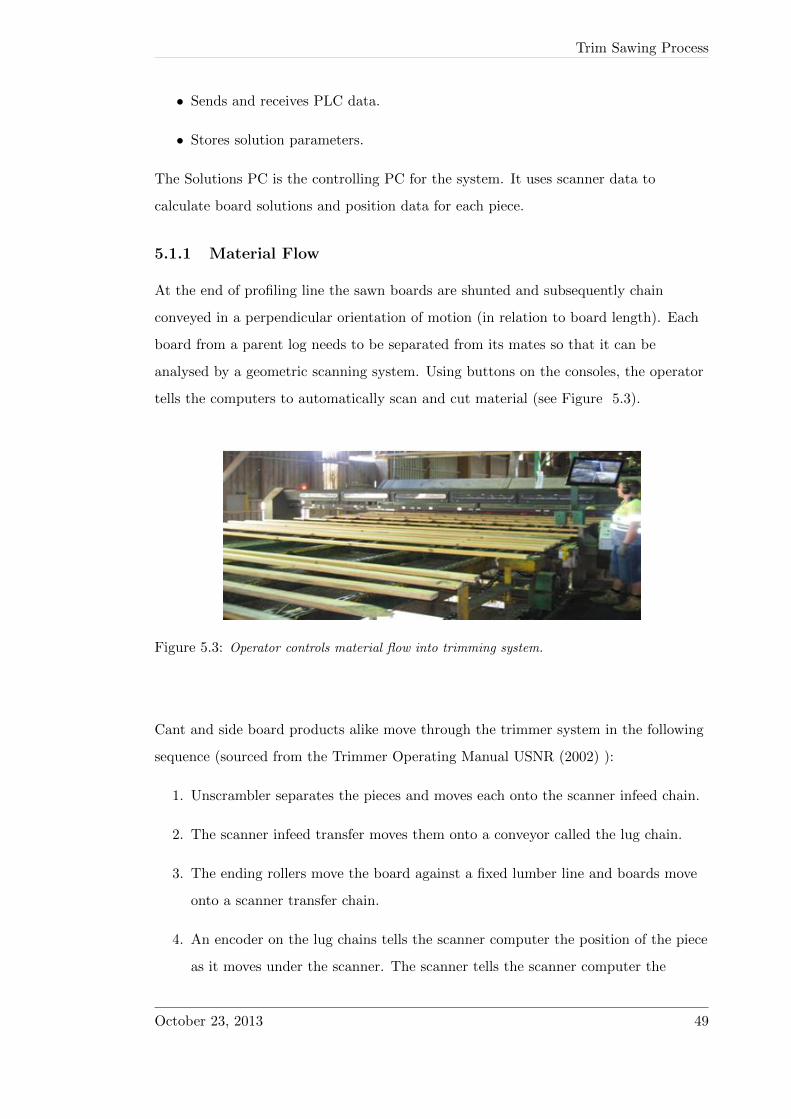
5.1.1 Material Flow
At the end of profiling line the sawn boards are shunted and subsequently chain
conveyed in a perpendicular orientation of motion (in relation to board length). Each
board from a parent log needs to be separated from its mates so that it can be
analysed by a geometric scanning system. Using buttons on the consoles, the operator
tells the computers to automatically scan and cut material (see Figure 5.3).
Figure 5.3: Operator controls material flow into trimming system.
Cant and side board products alike move through the trimmer system in the following
sequence (sourced from the Trimmer Operating Manual USNR (2002) ):
1. Unscrambler separates the pieces and moves each onto the scanner infeed chain.
2. The scanner infeed transfer moves them onto a conveyor called the lug chain.
3. The ending rollers move the board against a fixed lumber line and boards move
onto a scanner transfer chain.
4. An encoder on the lug chains tells the scanner computer the position of the piece
as it moves under the scanner. The scanner tells the scanner computer the
October 23, 2013 49

Trim Sawing Process
thickness of the board. The scan data is sent to the solutions computer, refer to
Figure 5.4.
5. The length scanner tells the scanner computer the length and width of the board.
Data sourced from this length-cell is sent to the solutions computer. The scanner
computer generates a geometric picture of each piece of material for the solutions
computer.
Figure 5.4: Trimmer geometric scanning module.
6. The solution computer calculates the most valuable combination of boards and
chips that can be cut from each board.
7. After passing through the scanner, the lug chain moves the board through the
trim saws, producing a final board.
8. The boards are moved to the sorter. Using buttons on the consoles, the operator
tells the computers to automatically scan and cut material.
5.1.2 Trimmer Laser Sensing
There are two trimmers in the Tuan sawmill. The laser spacing on trimmer 1 is one
inch and on trimmer two is four inches. Trimmer one has 22 heads with 23 lasers on
each, trimmer two has 20 heads with six lasers on each (half heads are on top and half
on the bottom). The lasers in these trimmers are point lasers which means there are
October 23, 2013 50

Trim Sawing Process
blind spots along the length of the boards from the laser data. Both trimmers use
lasers in coordination with a light curtain (spacing on Trimmer one and Trimmer two
light curtain is 2.5mm). Lasers measure the thickness and the wane profile, the light
curtains measure the length and combination of lasers/light curtain measures the
width of the board.
Briefly (also refer to Figure 5.5 and Figure 5.6) the laser scanner module for trimmer
machine centre generates geometric representation data in following manner:
• Lasers emit beams of infrared light into the scan area.
• The laser beams reflect off the material surface and the cameras sense the
reflected light. The reflected laser beam angle and intensity corresponds to the
thickness of measured material.
• Centroid data is the reflection position on the camera and peak data is the
maximum intensity of the reflected beams. The scan head signal processor
encodes the camera centroid and peak data.
• A fiber optic cable transmits the data to a receiving card in the scanner processor.
Figure 5.5: Point lasers scanning a board as it moves through.
The slashed pieces of board (i.e. pieces removed by the trim saws) drop down between
the trimmer conveyor chains onto a belt that feeds into a chipper. Subsequently all
slashed board is converted into saleable wood chip.
October 23, 2013 51

Trim Sawing Process
Figure 5.6: Trimmer scan head block diagram.
Figure 5.7: Scanned and solutioned boards en-
tering the trim saws.
Figure 5.8: Trimmed boards exiting the trim
saw booth.
October 23, 2013 52

Trim Sawing Process
5.1.3 Trim for Wane Criteria
Wane allowances are programmed through the trimmer interface computer system.
These parameters can be edited at any time by production controllers to control the
wane quality characteristics of timber boards to be processed in an upcoming run.
When setting up for wane by board rules data entry and changes are made in the Face,
Edge and Area Wane tables of the trimmer control interface. Wane is the percentage of
wood that can be missing. For example, face wane of 25% means that 75% of the face
of the board must be good wood and 25% can be missing, see Figure 4.9.
Primary and secondary wane limits control the total combined length over which
threshold face and edge wanes are allowed to be present on any one board product.
These limits are applied in the sawmill trimming process and as such if limits are
exceeded trim saws will activate to cut a section of the board off so that the remaining
length meets the specified limits. Figure 5.7 and Figure 5.8 illustrate sawn boards first
moving into the trim saws and second exiting the saws as finished sawmill board
product. If a length section not greater than the minimum required board length
(usually around 2.4m) cannot, be solved along the full length of a scanned board then
trim saws at 150mm spacing along the length of the board will be activated to go down
and cut up the entire length of board.
Primary wane is allowed full length and secondary is allowed for a percentage of the
length. Typical primary and secondary limits are (30% face x 30% edge x 100% length)
and (33% face x 35% edge x 30% length). The program has already predicted the face
and edge wane at 150mm increments along the length of the sawn F1 sideboards. The
next step is to simulate how the trimmer systems are likely to treat each virtually
generated sideboard width based upon the wane rules. Consideration must also be
given toward the physical spacing of the trim saws which ultimately also has a bearing
on the recovered length.
October 23, 2013 53

Trim Sawing Process
5.1.4 Trim for Length Criteria
If a board is over the minimum required length but under the actual trim saw spacing,
it would be allowed through without trimming. If a board is over the actual trim saw
spacing, it would be docked to the actual trim saw spacing. Figure 5.9 and Figure 5.10
gives an internal top perspective and almost side view of trim saw elements. Short
barrel hydraulic cylinders provide the mechanical thrust to drop saws into a board for
cutting then retract the saw up and clear of the next board.
Figure 5.9: Top view of a trim saw elements. Figure 5.10: Isometric view of three trim saws.
Trim saw spacings do vary, but usually sits around what is supplied in Table 5.1.
Minimums also vary from one trimmer to the other, but sit around the +20mm mark,
except for 2.4 / 3.0 which are 2.415 and 3.018.
Table 5.1: Trim saw table
Board nominal trim length (m) 2400 3000 3600 4200 4800 5400 6000
Trim saw fixed position (m) 2420 3026 3632 4238 4844 5450 6056
Min. allowed board length (m) 2415 3018 3620 4220 4820 5420 6020
The optimisers have the capacity to solution 2 boards from any single input piece
however the trimming systems don’t have the hardware (mechanicals or control
system) to recover 2 pieces from 1 piece. The optimiser only considers a single product
October 23, 2013 54

Trim Sawing Process
output and so logically chooses the most valuable single product solution, usually this
will be the longest length, but not always. If there’s two possible positions for the same
product out (i.e. a 2.4 from either the near end or far end of a 6.0m input) it takes the
solution closest to the 0 line. Provided it meets the wane criteria, there’s no value
difference between a board with no wane and a board with maximum wane.
Each virtual sideboard is first processed through the wane rules. Later a determination
is done on how well the remaining length fits with standard sawmill lengths so as to
ultimately determine which trim saw actuate down for the cross cut. Eventual yield for
that board at the trimmer is categorised into three:
1. Sawn board that will go to the sorter
2. Chip, which is produced from the docked sections and
3. Sawdust, which is produced by the sawcuts.
Given wane predictions at 150mm increments for F1 side boards for the various
potential widths, query is raised about handling the sections in between the points of
measurement. One way (also currently the way the program works) is to assume
uniformity of wane over the entire 150mm bucket. This is certainly the easiest way to
deal with the wane and reassuringly the trimmers do it this way. Slightly more
complicated manners would include assuming linear increase between end of bucket to
centre of preceding bucket data or effectively cut bucket sizes in half by assuming that
the plane where two data buckets join is the average of the 2 buckets.
October 23, 2013 55

Chapter 6
Virtual Product Volumation
6.1 F1 Sideboards
In terms of programming it is critical to understand that in a board length there can
be multiple regions that are distinguished by their resulting dimensional geometry
which ultimately can be graded into two separate classes being either:
1. Within wane tolerance specification, or
2. Outside wane tolerance specifications.
The developing simulation program has an existing inclination to sequence through the
log buckets using conditional ‘IF’ statements and counters. There are five standard
sawmill board widths that must be considered as potential sideboard candidates (refer
Table 3.1). Co-ordinated interaction between scanner system, computer and solutions
software, machine controller and the profiling machine creates the useful capability for
variable width sideboard recovery.
Imitating this process reveals that trimmer wane tolerances are vital to predicting the
best width sideboard to profile and saw from any particular log. Wane tolerances, both
Primary and Secondary have been discussed in the trimming process. If a board is sent
to the trimmer post profiling, sawing and if wane is found to exceed tolerance
specifications on any section of the board then the trim saws will be told to cut the
non conformance out. Recovered sawn yield is ultimately affected by what is docked at
the trimmer.
56
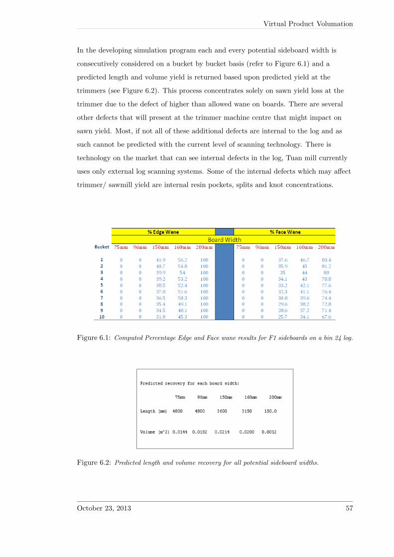
Virtual Product Volumation
In the developing simulation program each and every potential sideboard width is
consecutively considered on a bucket by bucket basis (refer to Figure 6.1) and a
predicted length and volume yield is returned based upon predicted yield at the
trimmers (see Figure 6.2). This process concentrates solely on sawn yield loss at the
trimmer due to the defect of higher than allowed wane on boards. There are several
other defects that will present at the trimmer machine centre that might impact on
sawn yield. Most, if not all of these additional defects are internal to the log and as
such cannot be predicted with the current level of scanning technology. There is
technology on the market that can see internal defects in the log, Tuan mill currently
uses only external log scanning systems. Some of the internal defects which may affect
trimmer/ sawmill yield are internal resin pockets, splits and knot concentrations.
Figure 6.1: Computed Percentage Edge and Face wane results for F1 sideboards on a bin 24 log.
Figure 6.2: Predicted length and volume recovery for all potential sideboard widths.
October 23, 2013 57

Virtual Product Volumation
For the developing simulation program, considering primarily wane defect as explained,
if initially there is an in tolerance section followed by a section that is determined to be
not in tolerance then the program works to transfer the in tolerance bucket counter to
a storage account and then resets the original incrementing counter for new use. If a
new in tolerance section occurs along the length of a single board then the in tolerance
counter is always ready to accumulate new length sections. It is not useful to store an
in specification section length if it falls below the minimum sawmills length for board
production. Nominally this length is 2400mm.
Figure 6.3: Extract from program code that checks that good section of 96mm wide F1 sideboard
is longer than minimum standard length.
To simplify computations the number of buckets in each log are truncated to integer
level and hence the nominal rule of rejecting sections that are less than 2.4m is
convenient and robust. As shown in the program code sample in Figure 6.3 a counter
is not allowed to pass to storage unless it contains the equivalent bucket count to
construct a minimum length sawmill board. The practical sense of this law is that if in
the transition from an in-tolerance section of board to an out of tolerance section, the
counter is even ‘one’ count less than the 2.4m required, then the in tolerance section is
impacted by being aggregated to trimmer docking. Subsequent yield is converted to
chips and sawdust (sawn residue). When the processing of an individual logs buckets is
completed then storage counters and live counters need to be compared against each
other to find the longest length for recovery.
October 23, 2013 58

Virtual Product Volumation
6.1.1 Total Sideboard Volume
If aggregation, tracking and reporting of length sections destinations is multifarious
enough then the associated volume calculation process is more so. Without any wane
board cross-section is a simple rectangle. Incorporate wane at a corner or on either
face or edge of the board and level of algorithmic involvedness needed to solve the
board cross-section area grows. Computing volume for out of specification sections is
as important to a yield simulation program as is the calculation of sections of sawn
board with no wane defect.
The code actively works on two independent pathways. Firstly every bucket of a board
is volumated regardless of the wane defect. This first round of volume calculations does
not pass nor fail a section of board but merely works to calculate a boards absolute
and total volume. Figure 6.4 is a sample taken from the simulation program code
showing how this process is executed. Discrimination at this point is applied in order
to have geometrically workable procedures in each instance, see Figure 6.10. The basis
of this discrimination is on which corners of the sawn board are affected by wane,
diagrams of four of the five cases are given in Figure 6.5 to Figure 6.8.
The fifth case is of course where there is no wane and the cross-section is easily
determined as a rectangle. In the other four instances the cross-section is divided into
geometric sections so that the area of each section can be independently determined.
The corners of each component shape are located by co-ordinate system using standard
x and y axis, where the virtual centre of the log is origin. Total cross-sectional area is
then computed by summing the component sections.
Since there is the underlying supposition that log bucket cross-sections are circular
then intersection co-ordinates of board lines with the outer perimeter of the log can be
found, (see Figure 6.11). This is very useful in computation of the sectional
components of cross-sectional area. Take for example the calculation of the area of the
segment separated by the chord created when the board has wane. The mathematical
solution: connect the circle’s centre to the two sides of the chord to obtain a sector of
the circle separated by two radii (see Figure 6.12). The angle of this sector is calculable
from the length of the chord and the radius and hence its area is known. The segment
October 23, 2013 59

Virtual Product Volumation
Figure 6.4: Extract of program code showing volumation of sideboard sections.
Figure 6.5: Face wane < 100% and Edge wane < 100%.
October 23, 2013 60
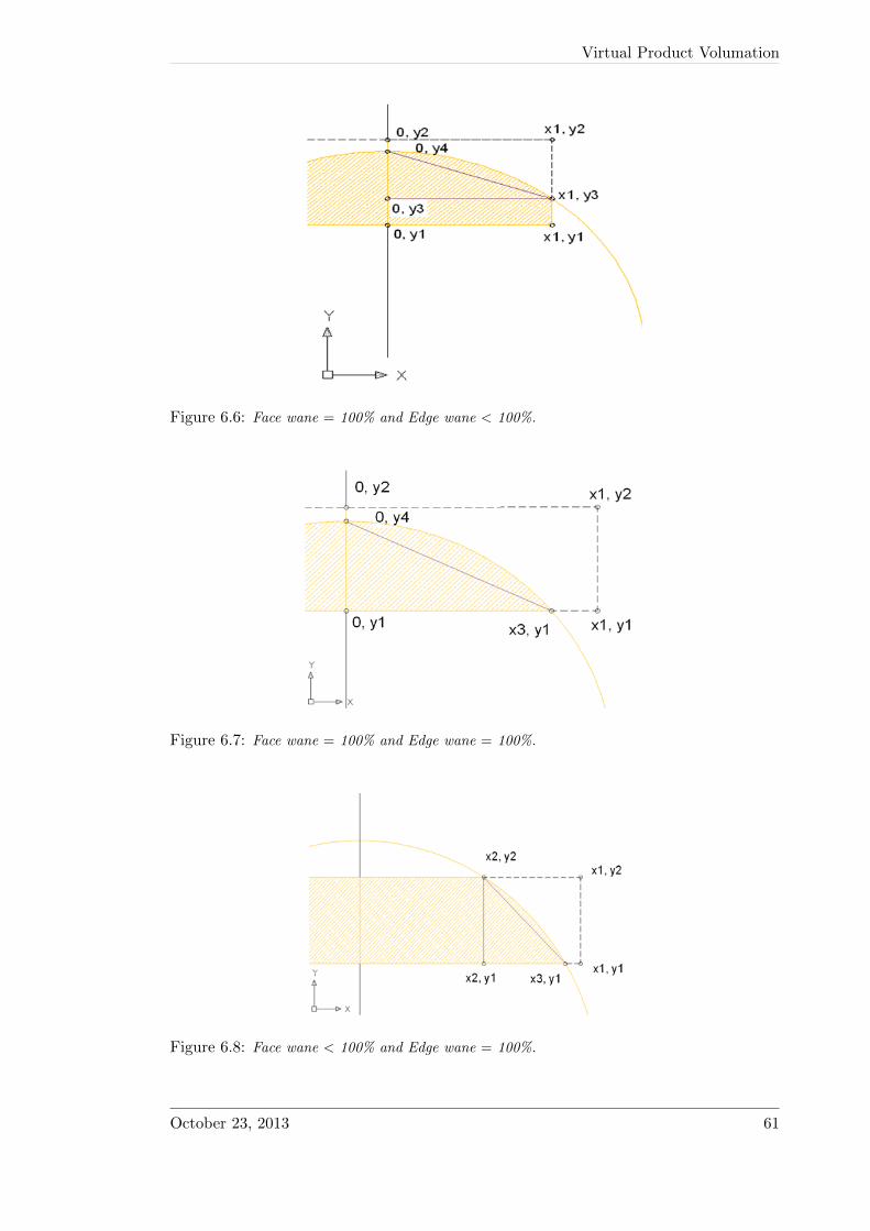
Virtual Product Volumation
Figure 6.6: Face wane = 100% and Edge wane < 100%.
Figure 6.7: Face wane = 100% and Edge wane = 100%.
Figure 6.8: Face wane < 100% and Edge wane = 100%.
October 23, 2013 61

Virtual Product Volumation
Figure 6.9: Summary yields for potential F1 sideboard widths.
October 23, 2013 62

Virtual Product Volumation
Figure 6.10: Flowchart for volumating sawn board sections.
October 23, 2013 63

Virtual Product Volumation
area is the difference between the area of the sector and the isosceles triangle made by
the chord and the two radii.
For example the F1 sideboard option where Edge wane = 100% and Face wane < 100%:
F1 Cross-section Area = (Area 1 + Area 2 + Area by Chord) × 2
Area 1 = (y2 − y1) × x2
Area 2 = 0.5 × ((x3 − x2) × (y2 − y1))
Figure 6.11: Area grouping for F1 sideboard when Face wane < 100% and Edge wane = 100%
Chord
Length = (sqrt(y2 − y1)
2 + sqrt(x3 − x2)2
θ = acos((2 ×Radius2 − Length2)/2 ×Radius2)
Area = (Radius2/2 × (θ − sin θ)
October 23, 2013 64

Virtual Product Volumation
Figure 6.12: Chord formed by the corners of the F1 sideboard.
6.1.2 Sideboard Volume Within Wane Tolerances
This refined volumation process integrates two filters built in to categorize those
sections that pass the primary wane test, those sections that pass the secondary wane
test and sections that fail both of the prior. This is working out which section to store
as likely sawn yield and which sections to store as likely chip yield, basis of which is
how the trimmer is programmed to make decisions. This volumation process is
intrinsically tied into the coded length recovery procedure. Figure 6.9 & Figure 6.2
shows a sawmill predicted yield summary for the full range of F1 sideboard widths.
6.2 Cant Products
The cant products make up a significant proportion of a sawmill patterns overall
volume. Figure 4.5 is a cross-sectional view of the cant products from the cut pattern
shown in Figure 4.4. The sawmill yield simulation program has been designed to
process outer cant products (like the two 40 x 76 in Figure 4.4) in a similar manner as
the F1 side boards were shown to be evaluated. Hence the program processes every log
bucket diameter to determine the percentage edge and face wane, Figure 6.14 and
Figure 6.15 demonstrates the general process by which the simulation software works
to divide the outer cant board cross-sections of each 150mm bucket in order to
accurately compute area and eventually the bucket volume. The cross-sectional
October 23, 2013 65

Virtual Product Volumation
Figure 6.13: Flowchart for volumating within wane specification sections of sideboard
October 23, 2013 66

Virtual Product Volumation
breakup process is determined by edge and face wane categorization, similar to that
explained for the F1 sideboards which, occurs (within the software filtering processing)
for every 150mm bucket section.
Figure 6.14: Segmenting the right outer side-
board for computing area.
Figure 6.15: Cartesian co-ordinates are applied
for geometric computation of outer cant board
area.
Total length recoverable (considering also trimmer parameters refer Table 5.1) and
volume are processed and then lengths and volumes passing the primary and secondary
wane rules are computed. The 100 x 76 centre cant product is handled a little
differently in that it is assumed that there will not be any wane on a product situated
in this region of a pattern or log. Hence the only particular issue affecting yield that
can and is re-created in the virtual yield simulator is to focus on trimmer length
categories.
October 23, 2013 67
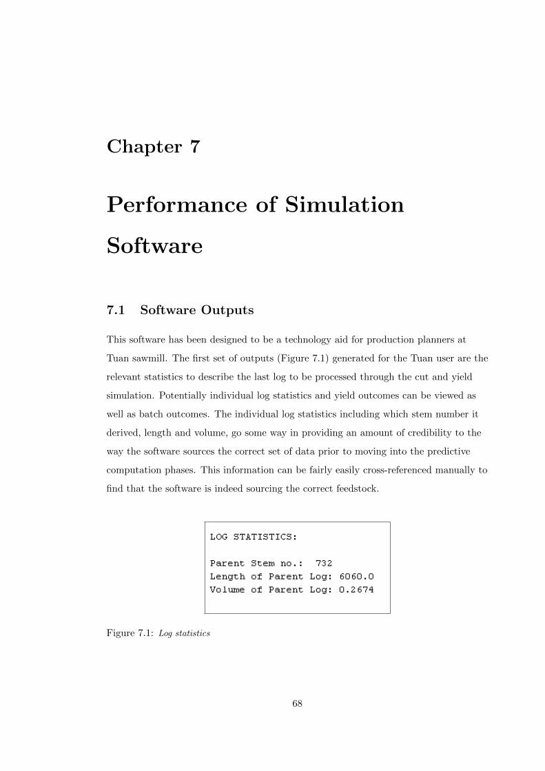
Chapter 7
Performance of Simulation
Software
7.1 Software Outputs
This software has been designed to be a technology aid for production planners at
Tuan sawmill. The first set of outputs (Figure 7.1) generated for the Tuan user are the
relevant statistics to describe the last log to be processed through the cut and yield
simulation. Potentially individual log statistics and yield outcomes can be viewed as
well as batch outcomes. The individual log statistics including which stem number it
derived, length and volume, go some way in providing an amount of credibility to the
way the software sources the correct set of data prior to moving into the predictive
computation phases. This information can be fairly easily cross-referenced manually to
find that the software is indeed sourcing the correct feedstock.
Figure 7.1: Log statistics
68

Performance of Simulation Software
7.1.1 Sideboard Yield
Sideboard yield has significant potential to affect the sawmill yield outcomes for any log
and batch of logs. There is flexibility built into control software and profiler machinery
movement to allow the width of sideboards to change from one log to the next. This
same degree of dynamic behaviour has been created in the yield software. When the
software is computing yields, the sideboard option priority (in the default state) is set
to maximise the potential sawn volume yielded from a sideboard set. Figure 7.2
demonstrates the comprehensive range of indicators the software can currently provide
in relation to a set of F1 sideboards for any log and pattern combination.
This set of indicators explain the source of chip and sawdust production in terms of
whether it has come from the Sawmill-line or the Trimmer. This allows for
comprehensive analysis of trimmer activity. The F1 sideboard width that has been
determined as the highest volume sawn yield option and their predicted length is
displayed in these results.
Figure 7.2: F1 sideboard yield indicators
7.1.2 Cant Products Yield
The width and thickness of the cant boards is locked and controlled only by the cut
pattern code, still there is no guarantee that any log will be a good fit for a designated
pattern. The simulator assumes that inside cant boards will always be a good fit for a
pattern, running on the reasonable assumption that the user is at least competent
October 23, 2013 69
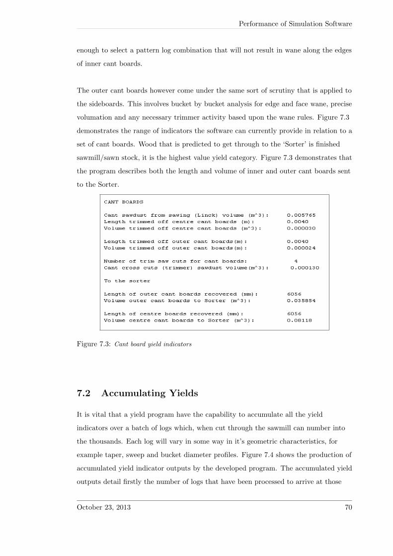
Performance of Simulation Software
enough to select a pattern log combination that will not result in wane along the edges
of inner cant boards.
The outer cant boards however come under the same sort of scrutiny that is applied to
the sideboards. This involves bucket by bucket analysis for edge and face wane, precise
volumation and any necessary trimmer activity based upon the wane rules. Figure 7.3
demonstrates the range of indicators the software can currently provide in relation to a
set of cant boards. Wood that is predicted to get through to the ‘Sorter’ is finished
sawmill/sawn stock, it is the highest value yield category. Figure 7.3 demonstrates that
the program describes both the length and volume of inner and outer cant boards sent
to the Sorter.
Figure 7.3: Cant board yield indicators
7.2 Accumulating Yields
It is vital that a yield program have the capability to accumulate all the yield
indicators over a batch of logs which, when cut through the sawmill can number into
the thousands. Each log will vary in some way in it’s geometric characteristics, for
example taper, sweep and bucket diameter profiles. Figure 7.4 shows the production of
accumulated yield indicator outputs by the developed program. The accumulated yield
outputs detail firstly the number of logs that have been processed to arrive at those
October 23, 2013 70

Performance of Simulation Software
totals. Figure 7.5 is the plot of sawmill yields. Total volume yield for sawn, dust and
chip are accumulated for each consecutive log processed. The overall sawn recovery is
the percentage of wood fibre from all logs processed that is predicted to be yielded as
sawn material i.e. flow through the trimmer to the sorter.
Figure 7.4: Accumulated sawmill yield indicators
The final outputs are what the program is all about and that which is a provision for
predicting sawn inventory. This software function gives a predicted sawn output in
actual numbers of product cross-sections and lengths recoverable through saw milling a
batch of logs, see Figure 7.6. There is a counter in the program, currently named ‘bin
24 counter’ which indicates how many logs have been processed through the yield
simulator in order to achieve the displayed sawn inventory. For the results displayed in
this section the batch sample size is 14 logs. It is significant that products are
differentiated on the basis of their location on the log (i.e. ‘Sideboard’, ‘Centre Cant’
or ‘Outer Cant’). Products sourced from the centre of a pine log are generally of lesser
quality, weaker strength rating and prone to warping whereas products from the
outside of the log are destined to be finished as high grade structural product.
7.3 Comparison of Software Yields and Actual Mill
Yields
Comparing actual sawmill sawn recovery for a full day (see Figure 7.7) with that
predicted by accumulated yield in the software batch log processing (Figure 7.4)
indicates a fairly reasonable match for percent sawn recovered, generally all in the
vicinity of 50%.
October 23, 2013 71

Performance of Simulation Software
Figure 7.5: Sawmill yield by log from simulator chart
October 23, 2013 72

Performance of Simulation Software
Figure 7.6: Predicted sawn stock
Figure 7.7: Sawmill actual sawn recovery sample
October 23, 2013 73

Performance of Simulation Software
Residue materials are separated out into sawdust and chip which are conveyed on
separate belts to designated bunkers. Each residue conveyor has a weigh scale fitted to
measure the rate of production. Figure 7.8 is typical production charted rates of
production supplied from the residue weigh scales. The blue line is a typical rate of
production (t/hr) for chips and the red line for sawdust production (t/hr). Notice that
in Figure 7.8 that the magnitude of chip production generally seems to be twice the
rate of sawdust production. Zooming into a typical section of the chart Figure 7.9
further supports the observation that in relative terms at the sawmill chip production
is approximately two times the production rate of sawdust.
What this means is that the predictive model is underestimating sawdust production
relative to chip production. Further analysis of the sawmill tooling indicates that the
saw segments in the profiling units may indeed be a source for this error because
currently the model produces only chip residue through the profiling units. Given that
there are saw segments top and bottom of profiling units to produce clean straight
edges, it is reasonable to assume saw kerf and associated sawdust production in the
profilers.
Figure 7.8: Sawmill residues production monitor chart
To make the appropriate substitution of sawdust generated by the profiler saw
segments requires further precision evaluation of cross-sectional areas. In this case it is
necessary to account for the cutting action of the profiler saw segments which in
between the top and bottom set of chipper knives of a profiler head (refer to
Figure 7.10). This equates to material sections 5mm either side of the F1 sideboards
and also outer can boards. In Figure 7.11 the purple shaded segments represent
October 23, 2013 74

Performance of Simulation Software
Figure 7.9: Rate of Chip production vs. rate of Sawdust production
sections that in the future need to be modelled as sawdust yield. In the current
software version these identified sections (in purple) are modelled as chip which result
in an inaccurate division of residue yield; higher than expected chip yield.
Figure 7.10: Profiler head
Figure 7.11: Addition of profiling saw segment kerfs from profiling units
October 23, 2013 75

Chapter 8
Summary of Findings and Future
Direction
A competitive foot hole in the softwoods saw milling industry relies upon sourcing,
adapting or developing technology features that either enhance the plant or
management capabilities. This is a capital intensive industry with all manner of
computer controlled process for handling the timber. It is easy for the casual observer
to underestimate the importance of being one or two steps ahead in terms of matching
up machine processes with the characteristics of the log stocks. One only need consider
that a one percent gain in optimized efficiency can add a magnitude of seven figures to
mill annual profit. The human brain or even experience alone cannot legitimately be
considered capable of handling these extreme rates of processing and decision making
without the aid of customised software. The literature review provided evidence that
some international regions (namely Finland and Canada) are well advanced in the
science of sawing simulation and further that these versions provide an element of
competitive advantage.
The log breakdown at Tuan mill has been covered in some detail ensuring a clear
understanding of all relevant machine processes and their application in the log
breakdown sequence. Matlab code has been written to simulate the log breakdown
process with particular attention given to the standard timber lengths and
cross-sections. There are numerous cut patterns for saw milling of logs dependant on
log batch characteristics and customer specified demand for product. The Matlab
76

Summary of Findings and Future Direction
algorithm interprets pattern codes and runs a comparison of ideal effective geometry vs
every 150mm bucket diameter of virtual input log. The added complication handled by
the program code was to search and find matches for a desired batch number and then
for each matched log retrieve the diameter bucket data from the corresponding parent
stem file.
Sideboard product computation was by far the most demanding aspect to code. Matlab
code predicts the interface of board extremities with the outer perimeter of each log
bucket and all potential board widths are checked for viability. For the purpose of this
investigation highest sawn volume return from sideboards was given priority.
The final simulation process centred on quality control through the trimmer stations.
Of particular interest here is the relative percentage of wane along any length of a
board compared against primary and secondary wane criteria. The trimmers are the
ultimate dictators of finished board length, the software imitates this responsibility.
For example an the software runs an internal check of trimmer saw spacing and
allowable tolerance ranges compared with predicted sawn timber length. Each trim cut
contributes dust from saw kerf and dockings are converted to chip.
Recommended projects to further the commercial value of this sawing simulation
software:
1. Log sweep algorithm;
2. Multi-batch comparative testing and analysis against real log runs;
3. Enhance graphical user interface;
4. Investigate and model energy consumption for log batches.
October 23, 2013 77

Bibliography
ABS 8731.0 (2013), ‘Building Approvals, Australia Febrary 2013’,
http://www.oesr.qld.gov.au. [Online; accessed April-10-2013].
Apthorp, B. (2013), ‘Improving efficiencies through the wood supply chain’,
http://www.fridayoffcuts.com/index.cfm?id=528no.2. [Online; accessed
31-May-2013].
Asikainen, K. & Panhelainen, A. (1970), ‘The effect of the ovalness of the log on the
sawing yield. (in finnish with english summary)’, Paper och Tra 6, 395–402.
Ertas, A. & Jones, J. C. (1996), The Engineering Design Process, John Wiley and
Sons, Toronto, Canada.
Lyhykainen, H., Makinen, H., Makela, A., Pastila, S., Heikkila, A. & Usenius, A.
(2009), ‘Predicting lumber grade and by product yield for scots pine trees.’, Forest
Ecology and Management 258, 146–158.
Maness, T. & Adams, D. (1991), ‘The combined optimization of log bucking and
sawing strategies.’, Wood Fiber Science 23, 296–314.
Song, T. & Usenius, A. (2007), Innosim - a simulation model of wood conversion chain,
in ‘Modelling the wood chain: forestry - wood industry - wood product markets’,
DCL Print and Signs, Helsinki, p. 183.
Todoroki, C. (1990), ‘Autosaw system for sawing simulation.’, New Zealand Journal of
Forestry Science 20, 332–348.
Todoroki, C. & Monserud, R. (2004), ‘Recovery from simulated sawn logs with sweep.’,
New Zealand Journal of Forestry Science 34(2), 190–205.
78

Bibliography
Todoroki, C., Monserud, R. & Parry, D. (2007), ‘Lumber volume and value from
elliptical western hemlock logs.’, Forest Product Journal 57(7/8), 76–82.
Todoroki, C. & Ronnqvist, M. (2002), ‘Dynamic control of timber production at a
sawmill with log sawing optimization.’, Scandinavian Journal of Forest Research
17, 79–89.
Usenius, A. & Heikkila, A. (2007), Woodcim - model system for optimization activities
throughout the supply chain, in ‘Modelling the wood chain: forestry - wood
industry - wood product markets’, DCL Print and Signs, Helsinki, p. 183.
USNR (2002), ‘Geo2 trimmer optimizer w/ timbergraphx’, [CD-ROM].
October 23, 2013 79

Appendices
80

Appendix A - Project Specification
University of Southern Queensland
Faculty of Engineering and Surveying
ENG4111/4112
TOPIC: Simulating Yield for Tuan Sawmill
SUPERVISOR: Kazem Ghabrie
ENROLMENT: Mechatronic Engineering
PROJECT AIM: This project will investigate the bucking and profiling processes at
Tuan Pine Manufacturing plant and highlight potential for improved all round
production planning by simulating crosscut logs into sawn yield at Tuan sawmill.
It is envisaged that initially a model computer program for a batch of logs belonging to
one user selected bin class will be developed in Matlab. This program shall work to
integrate a cut pattern code and Linck profiling line parameters to generate some yield
predictions. The initial model program will source log and stem data from a static file
provisioned from the company.
The program will filter the source file to find a user selected batch of logs, convert a
user selected profiling line cut pattern to dimensions and try to maximize sideboard
recovery.
SPONSORSHIP: HYNE & SONS TIMBER TUAN TRUEFRAME
PROGRAMME: Issue A, 24th March 2013
1. Investigate the data collected and stored in regards to the bucked logs. Source
database files from the Hyne Information Services Team.
2. Investigate and detail the Linck (brand) profiling line process to form an
understanding of what each machine centre does to the log and what effect that
has on the yield.
3. Write a program that can match any log back to the parent stem in the CSV file
in order to get the correct range of bucket diameter data. Use this micro-scale set
of diameters in the computation of processes affecting sawmill yield.
October 23, 2013 81

4. Over the length of an input log use a Matlab program to check the goodness of
fit for selected pattern relative to the cross-section of the log at 150mm (bucket)
intervals.
5. Look closely at the sideboard profiling process and write a Matlab program that
will search and find the widest possible sideboards (F1, F2, F3) that can fit the
pattern designated location; while considering primary and secondary face and
edge wane rules.
6. Investigate standard product lengths as controlled by the sawmill trimmers.
7. Use the Matlab program to maximise the length and volume of recovered
sideboards from a virtual trimming process.
8. Use the program to compute the length, cross-section and volume of simulated
sawn yield from a virtual log.
9. Use the program to compute the simulated chip and sawdust yield from a virtual
log.
10. Write into a Matlab program length control for simulated sawn product yield and
track the volume conversion from simulated sawn dockings to chip yield.
If time permits:
1. Integrate sweep parameter into the program.
2. Store a real batch of logs, process through the bucking system, collect the data
files, process through custom yield program then run the same batch of logs
through the sawmill and try to collect actual yield results. Compare the two and
suggest sources of variance.
3. Investigate Structured Query Language (SQL) and try to get the developing
simulation package integrated into current online and real time system.
October 23, 2013 82