Simulation based Evaluation of a Nonlinear Model PredictiveController for Friction Stir Welding of Nuclear Waste Canisters

Isak Nielsen1, Olof Garpinger2 and Lars Cederqvist3

Abstract— The Swedish nuclear waste will be stored incopper canisters and kept isolated deep under ground formore than 100,000 years. To ensure reliable sealing of thecanisters, friction stir welding is used. To repetitively producehigh quality welds, it is vital to use automatic control of theprocess. This paper introduces a nonlinear model predictivecontroller for regulating both plunge depth and stir zonetemperature, which has not been presented in literature before.Further, a nonlinear process model has been developed andused to evaluate the controller in simulations of the closedloop system. The controller is compared to a decentralizedsolution, and simulation results indicate that it is possible toachieve higher control performance using the nonlinear modelpredictive controller.

I. INTRODUCTION

The Swedish Nuclear Fuel and Waste Management Com-pany (SKB) is responsible for research and development of along term storage for Sweden’s nuclear waste. The proposedsolution consists of multiple protective barriers. The spentfuel is first encapsulated in 50 mm thick copper canisterswhich are then embedded in bentonite clay about 500 metersbelow ground in the Swedish bedrock, see Fig. 1.

The repository must keep the spent fuel safe for at least100,000 years until the radiation has decayed to safe levels.To ensure a sufficiently thick copper corrosion barrier, itis important that the canisters are sealed properly. SKB iscurrently investigating Friction Stir Welding (FSW) as amethod for sealing lids to the 5 m long and 1 m diametercanisters. The plunge depth and weld temperature must becontrolled within certain limits to produce the corrosionbarrier demanded by Swedish authorities. This is currentlyemployed using decentralized control consisting of a cas-caded temperature controller, Cederqvist et al. [2], togetherwith a newly proposed plunge depth controller, Nielsen etal. [10], with promising results.

However, cross couplings in the system together with up-per and lower bounds on the manipulated variables introducedifficulties with this control design, and the performancegains achieved using a Nonlinear Model Predictive Con-troller (NMPC) are investigated here.

1I. Nielsen is with the Department of Automatic Control, Insti-tute of Technology, Linkoping University, SE581 83 Linkoping, Swedenisak.nielsen@liu.se

2O. Garpinger is with the Department of AutomaticControl, Lund University, Box 118, SE-221 00 Lund, Swedenolof.garpinger@control.lth.se

3L. Cederqvist is with the Swedish Nuclear Fuel & Waste Man-agement Company, Grondalsgatan 15, SE-572 29, Oskarshamn, Swedenlars.cederqvist@skb.se

II. THE FRICTION STIR WELDING PROCESS

The sealing of the canisters is made using FSW, which isa solid state welding method invented in the early 90’s byThe Welding Institute (TWI), Thomas et al. [14]. This hasbecome a popular method for forging different metals, suchas aluminum, titan, steel and copper.

The basic setup in FSW is seen in Fig. 2, where twocopper pieces are welded. The rotating, non-consumable, toolconsists of a probe and a shoulder. It generates heat and whenthe metal is warm enough it is traversed along the joint line,stirring the material from the two pieces into a weld. Theheat is a result from friction and plastic deformation of thematerial.

In contrary to many regular FSW applications wherethe workpieces are relatively thin and flat, the sealing ofthe canisters involves thick, cylindrically shaped, metals. Apurpose-built welding machine, that copes better with highforces and torques than a standard FSW robot, was installedat the Canister Laboratory in Oskarshamn in 2003.

The tool used in SKB’s application consists of a probethat is approximately 50 mm long, and a convex scrollshoulder with a diameter of 70 mm. The choice of a convexshoulder instead of the commonly used concave shoulderwas investigated by Cederqvist et al. [4]. This choice givessmaller variations in plunge depth and spindle torque, whichis desirable from a control point of view.

Mayfield et al. [8] conclude that there are three axes inFSW, each with an effort and a flow. Either the effort orthe flow is manipulated while the other is determined bythe process. In SKB’s application, the axial force actingon the tool (Fz), the spindle rotation speed (ω) and thetool traverse speed (vw) are possible control signals. Thesevariables are depicted in Fig. 2. The corresponding variables

Fig. 1. Multiple protective barriers ensure a safe long term storage of theSwedish nuclear waste.

2013 European Control Conference (ECC)July 17-19, 2013, Zürich, Switzerland.

978-3-952-41734-8/©2013 EUCA 2074

Fig. 2. The manipulated variables are 1) Spindle rotation speed (ω),2) Traverse speed (vw) and 3) Axial force acting on the tool (Fz). Theupper part is the lid, and the lower part is the canister.

Msp

Pz T

Fz ω

Fig. 3. The relation between the process variables and the manipulatedvariables in the process. The arrows represent which variables are influenc-ing the others.

plunge depth (Pz), spindle torque (Msp) and traverse force(Ft) are then given by the process. It was decided to keepthe traverse speed constant at vw = 86 mm/min and use theother two variables as control signals since their influenceon the temperature and plunge depth is greater. The stirzone temperature (T ) and power input (P ) are also veryimportant process variables. The power input is determinedby multiplying spindle torque with spindle rotation speed.

Fig. 3 shows how the process variables are related. Theplunge depth affects the spindle torque, which in turn influ-ences the stir zone temperature. The plunge depth depends onthe temperature and, hence, there is a triangle of dependencesbetween the process variables. Changing the axial force willaffect both plunge depth and spindle torque, while the spin-dle rotation speed influences the temperature. Observationsreveal that the spindle rotation speed influences the torqueas well, but this is not accounted for in this article. Similarobservations were made by Cui et al. [5].

III. MODELING OF THE FRICTION STIRWELDING PROCESS

The combined plunge depth and stir zone temperaturecontrol is crucial at the welding sequence start-up, and hencethe model is derived for this initial sequence of the weldprocess. The model relates the two manipulated variablesto the controlled variables and is based on a torque modelproposed by Schmidt [12]. This torque model is combinedwith a linearized temperature model and a modified linearplunge depth model.

A. Plunge Depth Modeling

The plunge depth model proposed in this paper is based onrheology models that are approximate descriptions of visco-elastic materials, and metals at high temperatures can bemodeled as such, Flugge [6]. Experimental observations ofthe SKB data shows that the copper has a tendency to creep,which means that the metal continues to deform even undera constant force.

The tool is considered a rigid body that does not deformat all. Furthermore, it is assumed that the copper closestto the tool have a homogeneous temperature and that thecopper outside this region is completely stiff. The strain ε(t)is described by

ε(t) = c ·∆l(t), (1)

where ∆l(t) is the deformation of the material and c is aconstant. By assuming that the contact area is constant, thestress σ(t) can be expressed as

σ(t) =Fz(t)

A, (2)

where A is the contact area and Fz(t) is the force actingon the tool. The deformation is the same as the deviation inplunge depth, i.e.

∆l(t) = zSD(t)− zSD, (3)

where zSD is the shoulder depth (plunge depth minus probelength) and zSD is the shoulder depth around which thesystem is linearized.

The model is based on a 3-parameter fluid model, wherethe idea is to describe the deformation as a combination oftwo dash-pot elements and one spring element, Flugge [6].The relation between strain and stress then becomes,

σ(t) + p1σ(t) = q1ε(t) + q2ε(t), (4)

where p1, q1 and q2 are constants. Using these equationsand the fact that the movement of the tool is subjected toNewton’s second law gives

∆l(s) =1

mp1· 1 + p1s

s(s2 + Aq2+m

mp1s+ Aq1

mp1

)︸ ︷︷ ︸

GD(s)

∆Fz(s), (5)

as the relation between the change in force and the changein plunge depth. Here, m is the mass of all moving parts and∆Fz(s) = Fz(t) − Fz is the deviation in axial force fromthe linearization point Fz .

Observations have shown that the plunge depth is depen-dent on stir zone temperature as well as the applied axialforce. A varying temperature changes the hardness of theheated copper and hence also the parameters consideredconstant in (5).

This temperature dependence will be included in thefinal model as an ad hoc solution using a correction factormultiplied with the shoulder depth. The correction factoris assumed affine in the temperature deviation from sometemperature T , and it was estimated using the least-squares

2075

0 5 10 15 20 25−0.05

0

0.05

0.1

0.15

0.2

Time (s)

Del

ta l

(mm

)Validation of depth model

ModeledMeasured

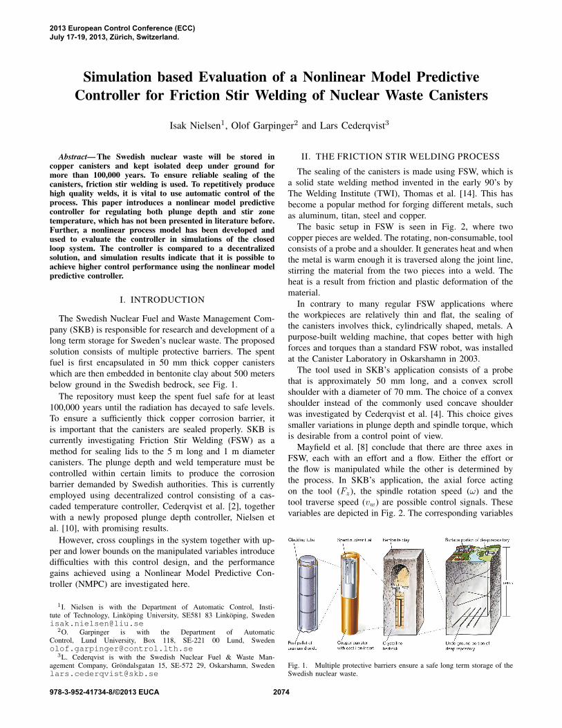
Fig. 4. Validation of the linearized plunge depth model. The model isvalidated for a step upwards followed by a step downwards in axial force.

method from a data set with constant axial force and varyingtemperature. The computed correction factor is

CF (∆T ) = 1 + 0.0021 ·∆T, (6)

where ∆T = T − T is the deviation in temperature.Using SYSTEM IDENTIFICATION TOOLBOX in MATLAB,

the linear rheology model combined with the correctionfactor gives the complete model

∆l(s) =0.0016 · (1 + 29.6s)

s (1 + 14.7s) (1 + 0.00095s)∆Fz(s)

zSD(t) = (∆l(t) + zSD) (1 + 0.0021 ·∆T (t)) .

(7)

The validation of this model is seen in Fig. 4 where a 4 kNstep upwards in axial force at 5 seconds is followed by a 4kN step downwards at 13.5 seconds.

B. Torque

The torque sensor measures the motor current and trans-lates it into motor torque (Mm). This must be compensatedfor in the control system since there is dissipation in themotor and transmission as a result of e.g. friction. Hence, thetorque measured by the sensor is a composition of frictiontorque and spindle torque. The friction torque was measuredrunning the process in air and a friction model is given by

Mf (ω) = 243.11− 1.305 · ω + 0.001927 · ω2. (8)

The torque exerted by the tool will be described usinga model by Schmidt [12], where the torque is produced intwo different ways; slipping and sticking. The slipping, orsliding, condition is when the tool velocity is higher thanthe material velocity at the interface, resulting in a Coulombfriction between the tool and the copper. When the stickingcondition is active, the material is assumed to rotate withthe tool and the torque is produced by shear stresses due toplastic deformation of the material. Schmidt et al. [12] arguethat it is a combination of these two conditions that togetherproduces the torque. Qian et al. [11] observed that the ratio

of torque produced by sticking and slipping conditions variesover a whole weld. In this paper, however, a constant ratiois used.

Introducing the constant state parameter δ ∈ [0, 1] thusgives

Msp = δMst + (1− δ)Msl, (9)

as the relation for spindle torque. Here Mst is the contribu-tion from the sticking condition and Msl is the contributionfrom the sliding condition. Looking at an infinitesimal partof the tool, the contact torque dMc is described by

dMc = r · dF = r · τc · dA, (10)

where τc is the contact shear stress (either τst or τsl), r isthe radius and dA is an infinitesimal area section. Integratingthis over the tool surface yields

Mc = G(zSD) · τc, (11)

where the geometric quantity G(zSD) is dependent on thetool as well as the plunge depth. The sliding shear stress isgiven by the Coulomb friction τsl(t) = µσ(t), where µ is thecoefficient of friction and σ(t) is the contact pressure. Thesticking shear stress is assumed to be the same as the copperyield stress, giving τst = τyield where τyield is assumedconstant in the relatively narrow band of temperatures usedhere. The contact pressure σ(t) is calculated as force dividedby area;

σ(t) =Fz(t)

A(zSD(t)), (12)

where A(zSD) is the depth dependent area given by the tool’sprojection on the canister surface. Together, these equationsgive

Msp(t) = (δτyield + (1− δ)µσ(t)) ·G (zSD(t)) (13)

as an expression for spindle torque.In the equations above, the combined inertia of the motor

and transmission was not considered. This inertia will actas a low-pass (LP) filter on the measurements. Hence, anLP-filter is added in the motor torque model, giving

τMMm = −Mm +Msp +Mf , (14)

where τM is the time constant of the filter and is estimatedfrom data.

C. Stir Zone Temperature

The heating of the stir zone is complex but can be approxi-mated with a linear differential equation relating temperatureto power input, see e.g. Cederqvist et al. [3] and Mayfieldet al. [8].

Experimental data from the initial sequence of a weld inthe lid were used to fit linear process models of varyingorders using MATLAB SYSTEM IDENTIFICATION TOOLBOX.The second order linear model with dead time

GT (s) =18.1

(1 + 30.5s)(1 + 1.2s)e−2.8s,

2076

gave the best fit. The estimation data consisted of stepresponses in spindle rotation speed while the axial force washeld constant.

It is a hypothesis of the authors that the temperature modelis actually two models in series; a first order differentialequation describing the heating of the copper, and anotherdescribing the heating of the tool. The thermo-couple thatmeasures the temperature is placed inside the probe, andtherefore the tool temperature is measured, not the stir zonetemperature.

D. Full Model

The full model consists of the equations for the torque,the extended plunge depth model and the temperature model.The linear models are linearized around points which corre-sponds to values that are representative when the controlleris active. These values are

Fz = 78.4 kN, T = 816.4◦CzSD = 2.66 mm, P = 43.6 kW

(15)

and the resulting, full model is (omitting time arguments forbrevity)

∆T =18.1

(1 + 30.5s)(1 + 1.2s)e−2.8s∆P (16)

∆l =0.0016 · (1 + 29.6s)

s(1 + 14.7s)(1 + 0.00095s)∆Fz (17)

0.27Mm = −Mm +Msp +Mf (18)Msp = (152800 + 0.435 · σ)G(zSD) (19)

σ =Fz

A (zSD)(20)

A (zSD) = π

(0.015 +

20

3zSD

)2

(21)

G (zSD) = 2.3 · 10−5 + . . .

. . .2.408 ·

((0.015 +

20

3zSD

)3

− 0.0153

)(22)

Mf = 243.11− 1.305 · ω + 0.001927 · ω2 (23)

∆P =(M −Mf )ωπ

30000− 43.6 (24)

Fz = ∆Fz + 78.4 (25)T = ∆T + 816.4 (26)

zSD = (∆l + 2.66)(1 + 0.0021 ·∆T ) (27)

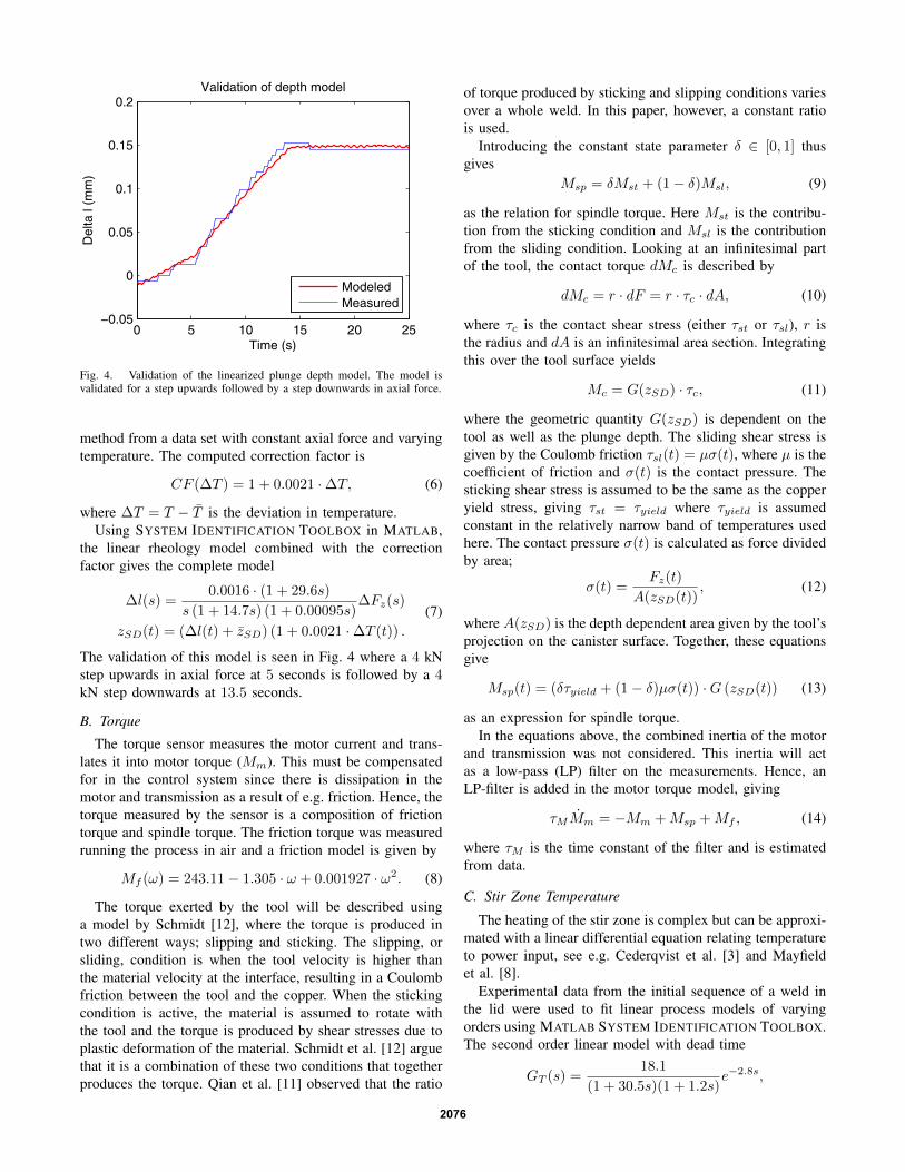
which will be used in the controller design. The validation ofthe model is seen in Fig. 5, where a 4 kN step in axial forceis applied at 2 seconds followed by a −4 kN step at 10.5seconds. A step of height 60 RPM is made in spindle rotationspeed at 19 seconds, followed by two −20 RPM steps at27.1 and 30.3 seconds. Since the torque measurements arederived from the motor current, there is a peak in the torqueafter approximately 20 seconds. This peak is a result of thespindle acceleration and is not injected to the process. Thecoupling between rotation speed and torque is seen after 20seconds. The measured torque drops, but since the model

0 5 10 15 20 25 30 35 402.6

2.7

2.8

2.9

3Depth

Time [s]

Sho

ulde

r de

pth

[mm

]

0 5 10 15 20 25 30 35 40810

820

830

840

850

860Temperature

Time [s]

Tem

pera

ture

[°C

]

0 5 10 15 20 25 30 35 401000

1050

1100

1150Torque

Time [s]

Tor

que

[Nm

]

MeasuredSimulated

MeasuredSimulated

Fig. 5. Validation of the full model. A step in the axial force is appliedfollowed by a step in spindle rotation speed. The model does not describethe relation between spindle rotation speed and torque.

does not capture this relation, the modeled torque is kept ata higher value. It is a hypothesis of the authors that this dropin torque is mainly due to the fact that the motor current isused as an indicator of torque. This conclusion is supportedby the modeled temperature which is still good, indicatingthat the torque drop is a sensor artifact and not due to a dropin spindle torque.

IV. NONLINEAR MODEL PREDICTIVE CONTROL

The basic idea when using linear or nonlinear MPC is tosolve an optimization problem to find the optimal controlsignal for some performance measure in in every iteration ofthe control loop. The simulations of the closed loop systemare made using the modeling, simulation and optimizationsoftware APMONITOR [1]. The continuous model presentedin Section III-D is discretized by APMONITOR and the useris not concerned with this matter.

The optimization problem consists of a cost function anda set of constraints that represents the nonlinear model andbounds on the manipulated variables. The cost function isa measure of how well the control performance goals aremet, and in this paper the L1 norm is used. This choiceis better at explicitly prioritizing the control objectives thanthe commonly used L2 norm, Hedengren et al. [7]. The ideawith this approach is to define a dead-band within which thecontrolled variable should be kept. If the value is outsidethis dead-band, it will be penalized by an increased cost.See e.g. Scokaert et al. [13] for a detailed explanation ofsoft constraints. Slack variables (ehi and elo) together with

2077

inequalities are introduced to relax the use of absolute values.This makes the cost function smooth and continuously dif-ferentiable which is a requirement for large-scale NonlinearProgramming (NLP) solvers. Besides the constraints givenby the model and limits on the variables, there are alsoconstraints for the upper and lower limits on the dead-band(yt,hi and yt,lo). The limits will be described by first orderlinear differential equations with time constants given by τt.This NLP problem is the same as in Hedengren et al. [7]with some weights equal to zero and no disturbance model,and has the form

minu

Φ = minu

wT ehi + wT elo + (∆u)T c∆u (28)

s.t. 0 = f(x, x, u) (29)0 = g(ys, x, u) (30)a ≥ h(x, u) ≥ b (31)

τt∂yt,hi∂t

+ yt,hi = sphi (32)

τt∂yt,lo∂t

+ yt,lo = splo (33)

ehi ≥ (ym − yt,hi) (34)elo ≥ (yt,lo − ym). (35)

The dynamic model is described by f(x, x, u) where x arethe states, u the control signal and ∆u the movement in u.The physical interpretation of x is not important since themeasurements ys and states are related by g(ys, x, u). Theconstraints on the control signals are given by the functionh(x, u) together with a and b. Further, the set points for theupper and lower limit of the dead band is given by sphi andsplo. The slack variables measure how far from the desiredtrajectory the modeled output ym is.

The optimization problem is solved over a finite timehorizon which has to be long enough to capture importantdynamics. The controller in this article uses the time horizon

t = [0 : 0.1 : 5, 7, 10, 15, 30]T , (36)

where MATLAB syntax has been used. The second part of thevector ([7, 10, 15, 30]T ) is added to get predictions furtherahead without adding a large number of extra variables tothe optimization problem.

The most important tuning parameters are the weights usedin the cost function, but also the time constant of the response(τt) is a tuning parameter that is set to 5 seconds here.The default solver in APMONITOR is APOPT, and the onlychanges to the default settings for this solver is the number ofnodes used in every prediction horizon which has been set to2 (default 4). The step sizes in the manipulated variables havebeen constrained to 1 kN and 3 RPM respectively, preventingexcessive movement in the control signals. The dead-bandsare set to ±0.1◦C from the desired stir zone temperature and±0.002 mm from the desired plunge depth, and the weights

w =

[1001

], c∆u =

[1

0.01

](37)

are used. These have been determined in an iterative manner.

0 50 100 150 200 250 3002.6

2.7

2.8

2.9Reference tracking

Time (s)

Sho

ulde

r de

pth

(mm

)

0 50 100 150 200 250 300815

820

825

830

835

Tem

pera

ture

(°C

)

Time (s)

ReferenceDecentralizedNMPC

ReferenceDecentralizedNMPC

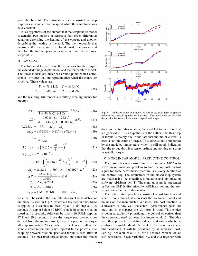
Fig. 6. Simulated controlled variables for the decentralized controller andthe NMPC. The NMPC almost completely decoupled closed loop system.The black lines are the references.

V. SIMULATION RESULTS

The proposed NMPC scheme has been compared in simu-lations to the implemented controller proposed in Nielsen etal. [10]. Results both from reference tracking and disturbanceaccommodation are presented here. Also, model uncertaintieshas been simulated giving results very similar to the distur-bance simulations. These are however not presented here.

A. Reference Tracking

The closed loop response for steps injected in plungedepth and stir zone temperature are seen in Fig. 6, withcorresponding control signals in Fig. 7. The NMPC schemeaccomplish an almost decoupled closed loop system, whereasthe decentralized controller has some significant interactionbetween the two controlled variables. The decoupling isachieved by compensating the cross-couplings by an activeuse of the control signal, see Fig. 7.

B. Disturbance Accommodation

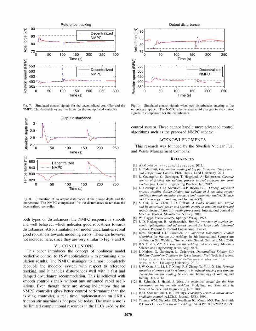
The closed loop systems have also been simulated fora step disturbance acting on the shoulder depth. This dis-turbance could be e.g. a sharp edge between the lid andthe canister which must be compensated for. The result isseen in Figs. 8 and 9. When the step disturbance is injected,the controllers make a quick drop in axial force, which theNMPC compensates with a quick increase in rotation speedto get a smooth descent. The decentralized controller, on theother hand, does not compensate as well which results in anundershoot. The fluctuations in depth induces changes in stirzone temperature which the decentralized controller cannotcompensate for immediately. A similar disturbance enters thetemperature at 160 seconds, with a similar behaviour. For

2078

0 50 100 150 200 250 30070

80

90

100A

xial

forc

e (k

N)

Time (s)

Reference tracking

0 50 100 150 200 250 300350400450500550

Rot

atio

n sp

eed

(RP

M)

Time (s)

DecentralizedNMPC

DecentralizedNMPC

Fig. 7. Simulated control signals for the decentralized controller and theNMPC. The dashed lines are the limits on the manipulated variables.

0 50 100 150 200 2502.7

2.8

2.9

3

Output disturbance

Time (s)

Sho

ulde

r de

pth

(mm

)

0 50 100 150 200 250820

830

840

850

Tem

pera

ture

(°C

)

Time (s)

DecentralizedNMPC

Fig. 8. Simulation of an output disturbance at the plunge depth and thetemperature. The NMPC compensates for the disturbances faster than thedecentralized controller.

both types of disturbances, the NMPC response is smoothand well behaved, which indicates good robustness towardsdisturbances. Also, simulations of model uncertainties revealgood robustness towards modeling errors. These are howevernot included here, since they are very similar to Fig. 8 and 9.

VI. CONCLUSIONSThis paper introduces the concept of nonlinear model

predictive control to FSW applications with promising sim-ulation results. The NMPC manages to almost completelydecouple the modeled system with respect to referencetracking, and it handles disturbances well with a fast anddamped disturbance accommodation. This is achieved withsmooth control signals without any unwanted rapid oscil-lations. Even though there are strong indications that anNMPC controller gives better control performance than theexisting controller, a real time implementation on SKB’sfriction stir machine is not possible today. The main issue isthe limited computational resources in the PLCs used by the

0 50 100 150 200 25075

80

85

90

Axi

al fo

rce

(kN

)

Time (s)

Output disturbance

0 50 100 150 200 250350400450500550

Rot

atio

n sp

eed

(RP

M)

Time (s)

DecentralizedNMPC

Fig. 9. Simulated control signals when step disturbances entering at theoutputs are applied. The NMPC scheme uses rapid changes in the controlsignals to compensate for the disturbances.

control system. These cannot handle more advanced controlalgorithms such as the proposed NMPC scheme.

ACKNOWLEDGMENTS

This research was founded by the Swedish Nuclear Fueland Waste Management Company.

REFERENCES

[1] APMONITOR. www.apmonitor.com, 2012.[2] L. Cederqvist, Friction Stir Welding of Copper Canisters Using Power

and Temperature Control, PhD. Thesis, Lund University, 2011[3] L. Cederqvist, O. Garpinger, T. Hagglund, A. Robertsson. Cascade

control of friction stir welding process to seal canisters for spentnuclear fuel. Control Engineering Practice, Jan. 2012.

[4] L. Cederqvist, C.D. Sorensen, A.P. Reynolds, T. Orberg. Improvedprocess stability during friction stir welding of 5 cm thick coppercanisters through shoulder geometry and parameter studies. Scienceand Technology in Welding and Joining 46(2).

[5] S. Cui, Z. W. Chen, J. D. Robson. A model relating tool torqueand its associated power and specific energy to rotation and forwardspeeds during friction stir welding/processing. International Journal ofMachine Tools & Manufacture 50, Sep. 2010.

[6] W. Flugge, Viscoelasticity, Springer-Verlag, 1975.[7] J. D. Hedengren, R. Asgharzadeh. Tutorial overview of solving dy-

namic optimization and advanced control for large scale industrialsystems. Preprint to Control Engineering Practice.

[8] D.W. Mayfield C.D. Sorensen. An improved temperature controlalgorithm for friction stir welding. In 8th International Symposiumon Friction Stir Welding, Timmerdorfer Strand, Germany, May 2010.

[9] R.S. Mishra, Z.Y. Ma. Friction stir welding and processing. MaterialsScience and Engineering R 50, Aug. 2005.

[10] I. Nielsen, O. Garpinger, L. Cederqvist. Decentralized Friction StirWelding Control on Canisters for Spent Nuclear Fuel. Technical report,http://urn.kb.se/resolve?urn=urn:nbn:se:liu:diva-91571 Linkoping University, 2013.

[11] J. W. Qian, J. L. Li, J. T. Xiong, F. S. Zhang, W. Y. Li, X. Lin. Periodicvariation of torque and its relations to interfacial sticking and slippingduring friction stir welding. Science and Technology of Welding andJoining, Jan. 2012.

[12] H. Schmidt, J. Hattel, J. Wert. An analytical model for the heatgeneration in friction stir welding. Modelling and Simulation inMaterial Science and Engineering, Nov. 2003.

[13] P. O. Scokaert and J. B. Rawlings. Feasibility issues in linear modelpredictive control. A.I.Ch.E. Journal, 45(8), 1999.

[14] Thomas WM, Nicholas ED, Needham JC, Murch MG, Temple-SmithP, Dawes CJ. Friction stir butt welding, Patent PCT/GB92/02203,1991

2079