Hybrid simulation theory for a classical nonlinear ...

UC BerkeleyUC Berkeley Previously Published Works

TitleHybrid simulation theory for a classical nonlinear dynamical system

Permalinkhttps://escholarship.org/uc/item/3wf5r15z

AuthorsDrazin, PLGovindjee, S

Publication Date2017-03-31

DOI10.1016/j.jsv.2016.12.034 Peer reviewed

eScholarship.org Powered by the California Digital LibraryUniversity of California

https://escholarship.org/uc/item/3wf5r15z

https://escholarship.org

http://www.cdlib.org/

Contents lists available at ScienceDirect

Journal of Sound and Vibration

Journal of Sound and Vibration ∎ (∎∎∎∎) ∎∎∎–∎∎∎

http://d0022-46

n CorrE-m

PleasJourn

journal homepage: www.elsevier.com/locate/jsvi

Hybrid simulation theory for a classical nonlinear dynamicalsystem

Paul L. Drazin a, Sanjay Govindjee b,n

a Department of Mechanical Engineering, University of California, Berkeley, Berkeley, CA 94720, United Statesb Department of Civil and Environmental Engineering, University of California, Berkeley, Berkeley, CA 94720, United States

a r t i c l e i n f o

Article history:Received 23 June 2016Received in revised form17 November 2016Accepted 20 December 2016

Keywords:Hybrid simulationHybrid simulation error analysisNonlinear dynamicsChaosLyapunov exponentLyapunov dimensionPoincaré section

x.doi.org/10.1016/j.jsv.2016.12.0340X/& 2016 Elsevier Ltd All rights reserved.

esponding author.ail addresses: [email protected] (P.L. Dra

e cite this article as: P.L. Drazin, & S.al of Sound and Vibration (2016), http

a b s t r a c t

Hybrid simulation is an experimental and computational technique which allows one tostudy the time evolution of a system by physically testing a subset of it while the re-mainder is represented by a numerical model that is attached to the physical portion viasensors and actuators. The technique allows one to study large or complicated mechanicalsystems while only requiring a subset of the complete system to be present in the la-boratory. This results in vast cost savings as well as the ability to study systems thatsimply can not be tested due to scale. However, the errors that arise from splitting thesystem in two requires careful attention, if a valid simulation is to be guaranteed. To date,efforts to understand the theoretical limitations of hybrid simulation have been restrictedto linear dynamical systems. In this work we consider the behavior of hybrid simulationwhen applied to nonlinear dynamical systems. As a model problem, we focus on thedamped, harmonically-driven nonlinear pendulum. This system offers complex nonlinearcharacteristics, in particular periodic and chaotic motions. We are able to show that theapplication of hybrid simulation to nonlinear systems requires a careful understanding ofwhat one expects from such an experiment. In particular, when system response is chaoticwe advocate the need for the use of multiple metrics to characterize the difference be-tween two chaotic systems via Lyapunov exponents and Lyapunov dimensions, as well ascorrelation exponents. When system response is periodic we advocate the use of L2

norms. Further, we are able to show that hybrid simulation can falsely predict chaotic orperiodic response when the true system has the opposite characteristic. In certain cases,we are able to show that control system parameters can mitigate this issue.

& 2016 Elsevier Ltd All rights reserved.

1. Introduction

Hybrid simulation (or hybrid-testing) is a popular experimental method that is primarily used in Civil Engineering la-boratories [1,2]. It originated roughly 30 years ago [3] and has been used continuously and extensively as a methodology toexperimentally assess structural systems under earthquake loadings. Occasionally the methodology has also been used inother disciplines to assess dynamic phenomena; see e.g. [4–6]. The central problem that hybrid simulation addresses is thatit is very difficult and expensive to test full-size civil structures for their structural capacities under seismic loads. The largesttesting facility in the world is the E-Defense facility [7] which can test structures with a 20 m�15 m plan and 12 MN

zin), [email protected] (S. Govindjee).

Govindjee, Hybrid simulation theory for a classical nonlinear dynamical system,://dx.doi.org/10.1016/j.jsv.2016.12.034i

www.sciencedirect.com/science/journal/0022460X

www.elsevier.com/locate/jsvi

http://dx.doi.org/10.1016/j.jsv.2016.12.034



mailto:[email protected]

mailto:[email protected]





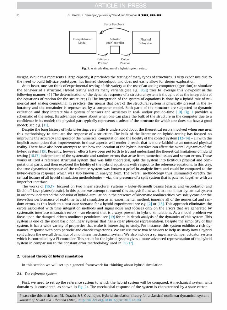
Fig. 1. A simple diagram of a hybrid system setup.

P.L. Drazin, S. Govindjee / Journal of Sound and Vibration ∎ (∎∎∎∎) ∎∎∎–∎∎∎2

weight. While this represents a large capacity, it precludes the testing of many types of structures, is very expensive due tothe need to build full-size prototypes, has limited throughput, and does not easily allow for design exploration.

At its heart, one can think of experimental testing of this variety as the use of an analog computer (algorithm) to simulatethe behavior of a structure. Hybrid testing and its many variants (see e.g. [8,9]) tries to leverage this viewpoint in thefollowing manner: (1) The determination of the dynamic response of a structural system is thought of as the integration ofthe equations of motion for the structure; (2) The integration of the system of equations is done by a hybrid mix of nu-merical and analog computing. In practice, this means that part of the structural system is physically present in the la-boratory and the remainder is represented by a computer model. Both parts of the structure are subjected to dynamicexcitation and they interact via a system of sensors and actuators in real- and/or pseudo-time [10]. Fig. 1 provides aschematic of the setup. Its advantage comes about when one can place the bulk of the structure in the computer due to aconfidence in its model; the physical part typically represents a subset of the structure for which one does not have a goodmodel; see e.g. [11].

Despite the long history of hybrid-testing, very little is understood about the theoretical errors involved when one usesthis methodology to simulate the response of a structure. The bulk of the literature on hybrid-testing has focused onimproving the accuracy and speed of the numerical computation and the fidelity of the control system [12–14] – all with theimplicit assumption that improvements in these aspects will render a result that is more faithful to an untested physicalreality. There have also been attempts to see how the location of the hybrid interface can affect the overall dynamics of thehybrid system [15]. Recently, however, efforts have been put forth to try and understand the theoretical limitations of hybridtesting [16,17] independent of the systematic and random errors that arise from numerical issues and sensor errors. Theseworks utilized a reference structural system that was fully theoretical, split the system into fictitious physical and com-putational parts, and then explored the fidelity of the hybrid equations with respect to the reference equations. In this way,the true dynamical response of the reference system was known a priori in analytic form and could be compared to thehybrid-system response which was also known in analytic form. The overall methodology thus illuminated directly thecentral feature of all hybrid simulation methodologies – viz., the presence of a split system that is patched together with animperfect interface.

The works of [16,17] focused on two linear structural systems – Euler-Bernoulli beams (elastic and viscoelastic) andKirchhoff-Love plates (elastic). In this paper, we attempt to extend this analysis framework to a nonlinear dynamical systemin order to understand the behavior of hybrid-simulation in the presence of kinematic nonlinearities. We solely consider thetheoretical performance of real-time hybrid simulation as an experimental method, ignoring all of the numerical and ran-dom errors, as this leads to a best case scenario for a hybrid experiment; see e.g. [2] or [18]. This approach eliminates theerrors associated with time integration methods and signal noise and focuses only on the errors that are generated bysystematic interface mismatch errors – an element that is always present in hybrid simulations. As a model problem wefocus upon the damped, driven nonlinear pendulum; see [19] for an in depth analysis of the dynamics of this system. Thissystem is one of the most basic nonlinear systems that has a clear physical representation. Despite the simplicity of thissystem, it has a wide variety of properties that make it interesting to study. For instance, this system exhibits a rich dy-namical response with both periodic and chaotic trajectories. We can use these two behaviors to help us study how a hybridsplit affects the overall dynamics of a nonlinear mechanical system. We also include a spring-mass-damper actuator systemwhich is controlled by a PI controller. This setup for the hybrid system gives a more advanced representation of the hybridsystem in comparison to the constant error methodology used in [16,17].

2. General theory of hybrid simulation

In this section we will set up a general framework for thinking about hybrid simulation.

2.1. The reference system

First, we need to set up the reference system to which the hybrid system will be compared. A mechanical system withdomain is considered, as shown in Fig. 2a. The mechanical response of the system is characterized by a state vector,

Please cite this article as: P.L. Drazin, & S. Govindjee, Hybrid simulation theory for a classical nonlinear dynamical system,Journal of Sound and Vibration (2016), http://dx.doi.org/10.1016/j.jsv.2016.12.034i




Fig. 2. (a) A general systemwith domain and state vector ( )tu x, . (b) A general systemwith imposed separation into two substructures for comparison tothe hybrid system. ∪ ∪ = and ∂ ∩ ∂ = .

P.L. Drazin, S. Govindjee / Journal of Sound and Vibration ∎ (∎∎∎∎) ∎∎∎–∎∎∎ 3

( ) ∈ ( )tu x x, for , 1

where t represents time. In order to compare the reference system response to the hybrid system response, we imagine thatthe reference system is split into two substructures: a “physical” substructure ( -side) and a “computational” substructure(-side) as shown in Fig. 2b, where ∪ ∪ = and ∂ ∩ ∂ = . The state vector can now be separated into two parts:

⎪

⎪⎧⎨⎩

( ) =( ) ∈

( ) ∈ ( )t

t

tu x

u x x

u x x,

, if

, if . 2

p

c

This defines the true response for a given mechanical system . The precise expression for ( )tu x, is found by determining thefunction that satisfies the governing equations of motion on and the imposed boundary conditions on ∂ .

2.2. The hybrid system

The response of the hybrid system should be defined in a similar fashion to make the comparison between the twosystems straight forward. Using the same boundary defined in Fig. 2b, the hybrid system is separated into two substructures,as seen in Fig. 3. In order to differentiate the reference system from the hybrid system a superposed hat (^) is used toindicate a quantity in the hybrid system. The mechanical response of the hybrid system is represented by the following statevector:

⎧⎨⎪⎩⎪

^( ) =^ ( ) ∈^ ( ) ∈ ( )

tt

tu x

u x x

u x x,

, if

, if . 3

p

c

In a hybrid system up and uc are determined from the “solution” of the governing equations of motion for and subjectedto the boundary conditions on ∂ and ∂ . The boundary conditions on ∂ ∩ ∂ and ∂ ∩ ∂ naturally match those of thereference system. However, in the hybrid system one must additionally deal with boundary conditions on the two interfacesides p and c , where = ∩ ∂p and = ∩ ∂c . The boundary conditions on p and c are provided by the sensor andactuator system.

The hybrid split leads to more unknowns than equations. To resolve this issue, we need a model of the actuator andsensor system. A relatively general form for such a model can be expressed as [16]:

Fig. 3. The hybrid system separated into the physical, , and computational, , substructures.





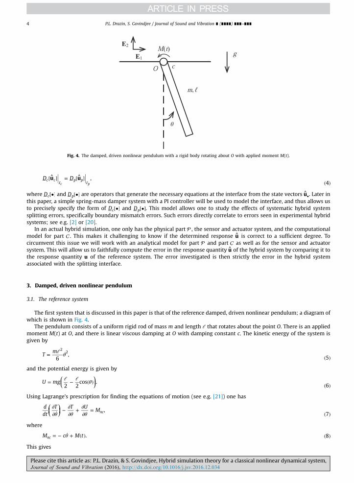
Fig. 4. The damped, driven nonlinear pendulum with a rigid body rotating about O with applied moment M(t).


[^ ] = [^ ]

( )D Du u ,

4c c p p

c p

where [•]Dc and [•]Dp are operators that generate the necessary equations at the interface from the state vectors ^•u . Later in

this paper, a simple spring-mass damper system with a PI controller will be used to model the interface, and thus allows usto precisely specify the form of [•]Dc and [•]Dp . This model allows one to study the effects of systematic hybrid systemsplitting errors, specifically boundary mismatch errors. Such errors directly correlate to errors seen in experimental hybridsystems; see e.g. [2] or [20].

In an actual hybrid simulation, one only has the physical part , the sensor and actuator system, and the computationalmodel for part . This makes it challenging to know if the determined response u is correct to a sufficient degree. Tocircumvent this issue we will work with an analytical model for part and part as well as for the sensor and actuatorsystem. This will allow us to faithfully compute the error in the response quantity u of the hybrid system by comparing it tothe response quantity u of the reference system. The error investigated is then strictly the error in the hybrid systemassociated with the splitting interface.

3. Damped, driven nonlinear pendulum

3.1. The reference system

The first system that is discussed in this paper is that of the reference damped, driven nonlinear pendulum; a diagram ofwhich is shown in Fig. 4.

The pendulum consists of a uniform rigid rod of mass m and length ℓ that rotates about the point O. There is an appliedmoment M(t) at O, and there is linear viscous damping at O with damping constant c. The kinetic energy of the system isgiven by

θ= ℓ ( )T

m6

, 5

22

and the potential energy is given by

⎜ ⎟⎛⎝

⎞⎠θ= ℓ − ℓ ( )

( )U mg

2 2cos .

6

Using Lagrange's prescription for finding the equations of motion (see e.g. [21]) one has

⎛⎝⎜

⎞⎠⎟θ θ θ

∂∂ − ∂

∂+ ∂

∂=

( )ddt

T T UM ,

7nc

where

θ= − + ( ) ( )M c M t . 8nc

This gives





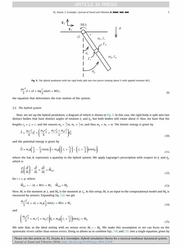
Fig. 5. The hybrid pendulum with the rigid body split into two pieces rotating about O with applied moment M(t).


θ θ θℓ ¨ + + ℓ ( ) = ( ) ( )m

c mg M t3 2

sin , 9

2

the equation that determines the true motion of the system.

3.2. The hybrid system

Next, we set-up the hybrid pendulum; a diagram of which is shown in Fig. 5. In this case, the rigid body is split into twodistinct bodies that have distinct angles of rotation θc and θp, but both bodies still rotate about O. Also, we have that the

lengths ℓ + ℓ = ℓp c , and the masses =ℓℓm mpp , = ℓ

ℓm mcc , and thus + =m m mp c . The kinetic energy is given by

⎛⎝⎜⎜

⎞⎠⎟⎟θ θ^ =

ℓ +ℓ

+ℓ + ℓ

( )T

m m m m

6 6 2,

10

c cc

p p c p p cp

22

2 2 22

and the potential energy is given by

⎜ ⎟⎛⎝

⎞⎠

⎛⎝⎜

⎛⎝⎜

⎞⎠⎟

⎛⎝⎜

⎞⎠⎟

⎞⎠⎟θ θ^ =

ℓ−

ℓ( ) + ℓ +

ℓ− ℓ +

ℓ( )

( )U m g m g

2 2cos

2 2cos ,

11c

c cc p c

pc

pp

where the hat, •, represents a quantity in the hybrid system. We apply Lagrange's prescription with respect to θc and θp,which is

⎛⎝⎜⎜

⎞⎠⎟⎟θ θ θ

∂ ^

∂ − ∂ ^

∂+ ∂ ^

∂= ^

( )

ddt

T T UM ,

12i i inci

for =i c p, , where

θ^ = − + ( ) + ^ = ( )M c M t M M M, . 13ncc c c ncp p

Here, Mc is the moment at c and Mp is the moment at p. In this setup, Mc is an input to the computational model and Mp ismeasured by sensors. Expanding Eq. (12) we get

θ θ θℓ ¨ + +

ℓ( ) = ( ) + ( )

mc m g M t M

3 2sin , 14

c cc c c

cc c

2

and

⎛⎝⎜⎜

⎞⎠⎟⎟

⎛⎝⎜

⎞⎠⎟θ θ

ℓ+ ℓ + ℓ ¨ + ℓ +

ℓ( ) =

( )

mm m m g M

3 2sin .

15

p pc p p c p p c

pp p

22 2

We note that, in the ideal setting with no sensor error, = −M Mc p. We make this assumption so we can focus on thesystematic errors rather than sensor errors. Doing so allows us to combine Eqs. (14) and (15) into a single equation, given by






⎛⎝⎜⎜

⎞⎠⎟⎟

⎛⎝⎜

⎞⎠⎟θ θ θ θ θ

ℓ ¨ +ℓ

+ ℓ + ℓ ¨ + +ℓ

( ) + ℓ +ℓ

( ) = ( )( )

m mm m c m g m g M t

3 3 2sin

2sin .

16

c cc

p pc p p c p c c

cc p c

pp

2 22 2

However, at this point, we only have one equation, Eq. (16), and two unknowns, θc and θp. To get a second equation, we needa model for the sensor and actuator system that connects the two bodies. For this paper, this is modeled as a spring-mass-damper system controlled by a PI controller; see e.g. [22]. The use a spring-mass-damper was chosen purely for its me-chanical simplicity and ease of understanding. The spring-mass-damper system can be easily used to introduce phase andmagnitude errors – known hybrid simulation errors [2,14,13] – at the hybrid interface while still allowing one to have ananalytical model that can be solved using standard numerical techniques, such as the Runge-Kutta methods. For the modelchosen, we follow the definition from the previous section for internal boundary conditions, or

[^ ] = [^ ]

( )D Du u .

17c c p p

c p

In this case uc and up are given by

⎡⎣ ⎤⎦ ⎡⎣ ⎤⎦θ θ^ = ^ = ( )u u, , 18c c p p

and the operators [^ ]D uc c and [^ ]D up p have the following definitions:

⎛⎝⎜

⎞⎠⎟( )[^ ] = + + + ^

( )D k k k k c k

ddt

c kddt

u u ,19

c c a i a p a i a p c

2

2

and

⎛⎝⎜

⎞⎠⎟( ) ( )[^ ] = + ( + ) + + ( + ) + ^

( )D k k k k c k

ddt

c kddt

md

dtu u1 1 ,

20p p a i a p a i a p a p

2

2

3

3

where the parameters ma, ca, and ka are the mass, damping constant, and stiffness of the spring-mass-damper system usedto model the actuator. The parameters kp and ki are the proportional and integral gains of the PI controller. Applying thesedefinitions ultimately leads to

θ θ θ θ θ θ θ¨ + ( + ) + = + ( ( + )) ¨ + ( ( + ) + ) +( )

…c k k k c k k k m c k k k c k k k1 1 .

21a p c a p a i c a i c ap

a p p a p a i p a i p

Thus, the equations of motion for the hybrid system are given by Eqs. (16) and (21). While the PI controller has been used inprevious works [5], it is emphasized that the PI controller is only used here for concreteness. The entire exercise is easilyrepeatable with alternate control methodologies; see e.g. [23,11]. The controller that one should employ in an actual ex-periment is based on the experimental setup that is used and one that minimizes errors that are important to problem athand (amongst those metrics that we highlight in the paper and perhaps others of physical significance to the researcher).For these reasons, alternative control schemes are not discussed further in this paper.

3.3. Non-dimensionalization

For further analysis, it is beneficial to non-dimensionalize Eqs. (9), (16), and (21). In order to do this, we define thefollowing non-dimensional quantities:

τ =ℓ ( )

tg

,22a

=ℓℓ

=ℓℓ ( )L L, , 22bc

cp

p

= = = = ( )Mmm

L Mm

mL, , 22cc

cc p

pp

γ =ℓ ℓ ( )

cm g

,22d

⎛⎝⎜

⎞⎠⎟

μ ττ

( ) == ℓ

ℓ ( )

M tg

mg,

22e






γ= = ℓ =ℓ

( )M

mm

cm g

Kkmg

, , ,22f

aa

aa

aa

= = ℓ( )

K k K kg

, .22gp p i i

Using Eq. (22) allows us to rewrite Eqs. (9), (16), and (21) as,

θτ

γ θτ

θ μ τ+ + ( ) = ( )( )

dd

dd

332

sin 3 ,23

2

2

⎛⎝⎜⎜

⎞⎠⎟⎟

⎛⎝⎜⎜

⎞⎠⎟⎟

θτ

θ

τγ

θτ

θ θ μ τ+ + + + ( ) + + ( ) = ( )( )

L d

d

LL L

d

d

dd

LL L

L

3 3 2sin

2sin ,

24

c c pc p

p c cc p c

pp

3 2

2

3 2

2

2 2

and

γθ

τγ

θτ

θθ

τγ

θ

τγ

θτ

θ+ ( + ) + = + ( ( + )) + ( ( + ) + ) +( )

Kd

dK K K

dd

K K Md

dK

d

dK K K

d

dK K1 1 .

25a pc

a p a ic

a i c ap

a pp

a p a ip

a i p

2

2

3

3

2

2

This gives us the non-dimensionalized equations of motion for the reference and hybrid systems.

4. Analysis

For the analysis, the applied moment is given by

μ τ μ Ωτ( ) = ¯ ( ) ( )cos , 26

where μ is the non-dimensional magnitude of the applied moment and Ω is the non-dimensional frequency of the appliedmoment. To start, the constants in the system are set as follows: =L 0.6c , Lp¼0.4, Ma¼0.5, γ = 0.1, γ = 25a , Ka¼12.5, Ki¼3,Kp¼10. Eqs. (23)–(25) are integrated numerically using the Dormand-Prince method, which is a type of the Runge-KuttaODE solver [24]. A tolerance of 10�7 was used when evaluating the Dormand-Prince method. This method is a standardmethod used to evaluate non-stiff equations with medium accuracy.

Since the reference forced pendulum is a two-state non-autonomous system, the system will exhibit either periodicmotion or chaotic motion depending on the values of the parameters, see [25]. The hybrid forced pendulum is a five-statenon-autonomous system and will also exhibit either periodic or chaotic motion. If the motion is periodic, the period of the

steady-state motion will be an integer multiple of the forcing period, nT , where = …n 1, 2, 3 and = πΩ

T 2 ; if >n 1, this cor-

responds to an excited subharmonic of period nT (see [26]). In order to determine the character of the motion of the systems,it is useful to employ the use of Lyapunov exponents; see [27]. If the largest Lyapunov exponent is positive, then the systemwill exhibit chaotic motion. If the largest Lyapunov exponent is 0, then the systemwill experience periodic motion; see [28].Also, as long as the sum of all of the Lyapunov exponents is negative, then we know that the system is stable in the sense ofLyapunov. The Lyapunov exponents are found using the QR method for small continuous nonlinear systems as outlined by[29] and the FORTRAN code provided by [30] – LESNLS – was modified to calculate the Lyapunov exponents for our systems.For a thorough discussion on the utility and implementation of the LESNLS code, please see Dieci et al. [29].

To begin, let us examine how the magnitude of the applied moment determines the behavior of the responses of both thereference and hybrid systems for a fixed frequency of the applied moment. We will set Ω = 1 for multiple values of μ. Fromthis, we will be able to determine when the systems are either periodic or chaotic. Fig. 6 shows the largest Lyapunovexponent for the reference and hybrid systems as a function of the forcing magnitude. From Fig. 6 we can see that, for themost part, the reference and hybrid systems exhibit the same type of behavior. However, there are a few instances when onesystem is periodic and the other is chaotic. This indicates that there are three separate cases that one needs to considerwhen performing an error analysis of a nonlinear hybrid simulation system: both responses are periodic, both responses arechaotic, and one response is periodic while the other is chaotic.

4.1. Periodic reference and hybrid systems

First we will analyze the case when both the reference and hybrid systems are periodic. For this case, we attempt toutilize L2 error to gauge how well the hybrid system is matching the reference system in the same manner as [16]. The L2

error is given by





Fig. 6. The Lyapunov exponents for the reference, λ1, and hybrid systems, λ1, when Ω = 1.


⎛⎝⎜⎜

⎛⎝⎜

⎞⎠⎟

⎞⎠⎟⎟

⎛

⎝⎜⎜

⎛⎝⎜

⎞⎠⎟

⎞

⎠⎟⎟

⎛⎝⎜

⎞⎠⎟

( )( )∫

∫τ

θ θ θτ

θτ

θ θ θτ

θτ

θ θτ

( ) =

− + − + − + −

+( )

τ

τ

E

Ldd

dd

Ldd

d

d

dd

.

27

c cc

p pp

2

0

22

22

02

2

Note that the L2 error used for the analysis is normalized with respect to the reference system. Also note that the differencein angles is always taken to be the smallest angular distance between 0 and π2 . We calculate the L2 error at three differentvalues of μ: μ = 0.7, 1.114, 2.6. A careful examination of Fig. 6 shows that all three of these values will produce periodicmotion in both systems. The L2 error time series for these three values of μ are shown in Fig. 7. This figure shows that whenthe transients are still present, small τ, the error varies rapidly. However, as τ increases, the error approaches a steady statevalue. This makes sense because both systems are approaching a periodic solution, thus the difference between the twosolutions should be approximately constant. However, as can be seen in Fig. 7, for μ = 1.114, the L2 error approaches a valuenear 1.3, or 130%. This indicates that the hybrid system is not tracking the reference system at all. Upon further study we findthat the reference system is traveling in a clockwise direction, while the hybrid system is traveling in a counter-clockwisedirection. Thus, the hybrid system is matching the response of the reference system, just in the opposite direction. This is the

Fig. 7. The L2 error for Ω = 1 for three values of μ with only periodic responses.





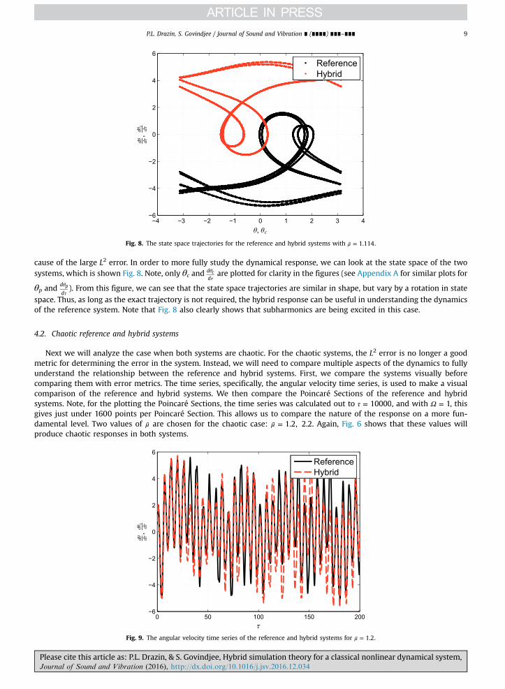
Fig. 8. The state space trajectories for the reference and hybrid systems with μ = 1.114 .


cause of the large L2 error. In order to more fully study the dynamical response, we can look at the state space of the twosystems, which is shown Fig. 8. Note, only θc and θ

τdd

c are plotted for clarity in the figures (see Appendix A for similar plots for

θp andθ

τ

d

dp ). From this figure, we can see that the state space trajectories are similar in shape, but vary by a rotation in state

space. Thus, as long as the exact trajectory is not required, the hybrid response can be useful in understanding the dynamicsof the reference system. Note that Fig. 8 also clearly shows that subharmonics are being excited in this case.

4.2. Chaotic reference and hybrid systems

Next we will analyze the case when both systems are chaotic. For the chaotic systems, the L2 error is no longer a goodmetric for determining the error in the system. Instead, we will need to compare multiple aspects of the dynamics to fullyunderstand the relationship between the reference and hybrid systems. First, we compare the systems visually beforecomparing them with error metrics. The time series, specifically, the angular velocity time series, is used to make a visualcomparison of the reference and hybrid systems. We then compare the Poincaré Sections of the reference and hybridsystems. Note, for the plotting the Poincaré Sections, the time series was calculated out to τ = 10000, and with Ω = 1, thisgives just under 1600 points per Poincaré Section. This allows us to compare the nature of the response on a more fun-damental level. Two values of μ are chosen for the chaotic case: μ = 1.2, 2.2. Again, Fig. 6 shows that these values willproduce chaotic responses in both systems.

Fig. 9. The angular velocity time series of the reference and hybrid systems for μ = 1.2.





Fig. 10. A zoomed in plot of the angular velocity time series of the reference and hybrid systems for μ = 1.2.

Fig. 11. The Poincaré Sections of the reference and hybrid systems for μ = 1.2.


Figs. 9 and 10 show the times series (of the angular velocities) for the systems with μ = 1.2 (see Appendix A for θ

τ

d

dp plots).

It is clear that the two systems do not track each other very well. However, looking at Fig. 11, which shows the PoincaréSections for both the reference and hybrid systems with μ = 1.2, we can easily see the similarity between the two PoincaréSections. This indicates that even when both systems are chaotic, the fundamental nature of the responses are nearlyidentical.

Next, we look at the case when μ = 2.2. The angular velocity time series are shown in Figs. 12 and 13, which show thatthe time series of the reference and hybrid systems match each other fairly well. However, the corresponding PoincaréSections, shown in Fig. 14, show very little correlation. Similar conclusions can be drawn from θp and θ

τ

d

dp as shown in

Appendix A. So, even though the time series match well, their Poincaré Sections do not. This confirms the need to examinemultiple aspects of the dynamics.

4.2.1. Chaos error metricsBesides the above described visual error analysis, we compute three different error metrics used to give a numerical

value to the error between two chaotic systems. First, we will compare Lyapunov exponents of the two systems. This allowsus to directly compare the level of chaos in each system, as the Lyapunov exponent defines how quickly trajectories willdiverge from each other due to small variations in the trajectories; see [31]. The second value we will compare is theLyapunov dimension, dL, which defines the dimension of the strange attractor and is calculated by





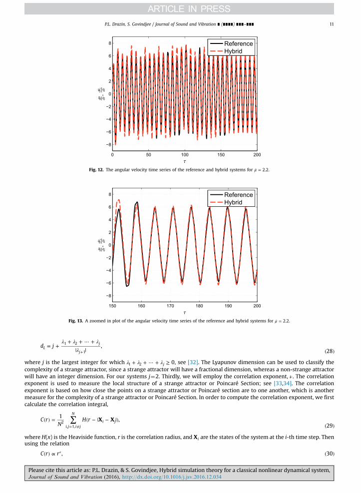
Fig. 12. The angular velocity time series of the reference and hybrid systems for μ = 2.2.

Fig. 13. A zoomed in plot of the angular velocity time series of the reference and hybrid systems for μ = 2.2.


λ λ λλ

= ++ + ⋯ +

| | ( )+d j ,

28L

j

j

1 2

1

where j is the largest integer for which λ λ λ+ + ⋯ + ≥ 0j1 2 , see [32]. The Lyapunov dimension can be used to classify thecomplexity of a strange attractor, since a strange attractor will have a fractional dimension, whereas a non-strange attractorwill have an integer dimension. For our systems j¼2. Thirdly, we will employ the correlation exponent, ν. The correlationexponent is used to measure the local structure of a strange attractor or Poincaré Section; see [33,34]. The correlationexponent is based on how close the points on a strange attractor or Poincaré section are to one another, which is anothermeasure for the complexity of a strange attractor or Poincaré Section. In order to compute the correlation exponent, we firstcalculate the correlation integral,

∑( ) = ( − | − |)( )= ≠

C rN

H r X X1

,29i j i j

N

i j2, 1,

where H(x) is the Heaviside function, r is the correlation radius, and Xi are the states of the system at the i-th time step. Thenusing the relation

( ) ∝ ( )νC r r , 30





Fig. 14. The Poincaré Sections of the reference and hybrid systems for μ = 2.2.


we can solve for the correlation exponent, ν. In this paper, the correlation exponent was calculated using the points in thePoincaré Section. The errors with respect to these three metrics are calculated as follows:

λ λλ

=| − ^ |

( )λerr ,31

1 1

1

=| − ^ |

( )err

d dd

,32d

L L

LL

and

ν νν

= | − ^|( )νerr . 33

where the hat, •, again, represents quantities for the hybrid system. Figs. 15–17 show these error measures versus appliedmoment magnitude. Note, points are only calculated for values of μ for which both the reference and hybrid system arechaotic.

Examining Fig. 15, we can see a wide variety of errors in the largest Lyapunov exponents, however, about half of all errorsare less than 0.2, or less than 20 %. This shows that about half the time the levels of chaos in both systems are equivalent, yet

Fig. 15. The error between λ1 and λ1 as a function of μ.





Fig. 16. The error in the Lyapunov dimension as a function of μ.

Fig. 17. The error in the correlation exponent of the Poincaré Sections as a function of μ.


there are times when the two systems vary greatly. Looking at Fig. 16, we see that all of the errors are below 0.4, and asignificant portion, more than nine-tenths, are less than 0.2. This shows that there is much less deviation between theLyapunov dimension of the reference and hybrid systems, indicating that the dimension of their strange attractors stay nearone another. From examining Fig. 17, we can see that there is a high density of points below 0.2, about two-thirds of allpoints are below 0.2. This shows that most of the time the Poincaré Sections of the two systems match fairly well, however,there are still instances in which the two systems do not match well. For the cases which we visually examined above,

=λerr 0.12031

, =err 0.1552dL, and =νerr 0.0526 when μ = 1.2, and =λerr 0.3680

1, = × −err 2.810 10d

4L

, and =νerr 0.2792 forμ = 2.2. These values again fit with our determination that multiple quantities are needed to properly assess the errorbetween two chaotic responses.

4.3. One system periodic and the other chaotic

The third case is when one system has a chaotic response and the other system has a periodic response. In this situationit is not possible to compare the two systems as the L2 error breaks down for chaotic systems, and the Poincaré Section for aperiodic system will be a single point, whereas the Poincaré Section for a chaotic system will be Cantor-like, see e.g. [35] or[25]. For these reasons, it is clear the correlation between the two responses will be nonexistent.





Fig. 18. The Lyapunov exponents for the reference and hybrid systems when Ki¼10.

Fig. 19. The E2herror as a function of Ki for multiple values of μ.


4.4. Study of Ki

All of the above analysis was done with specific values of the control parameters. If we instead use Ki¼10, which wasarbitrarily chosen, we can see how the Lyapunov exponents of the hybrid systemmatch those of the reference system muchbetter, as seen by comparing Figs. 6 and 18. This potentially indicates that if we increase the integral gain, Ki, we get bettermatching between the reference and hybrid systems. To investigate this further, we now look at the effects of changing theintegral gain, Ki. In the context of this paper, holding Kp constant and increasing Ki means the response of the controlledsystem is quicker, but it becomes more oscillatory and less stable [22]. Thus, as Ki increases, the magnitude error at thehybrid interface increases while the phase error decreases. However, it is noted that this only applies for the simple PIcontroller used in this paper. We will look at three specific values of μ:μ = 1.114, 1.2, 3.0. The first value was chosenbecause both the hybrid and reference systems were periodic at Ki¼3, but the hybrid system is going the opposite directionof the reference system. The second value was chosen because the response is chaotic for both systems at Ki¼3. And thethird value was chosen because the reference response is periodic, while the hybrid response is chaotic at Ki¼3. Foranalyzing the effect of changing Ki, we look at the hybrid L2 error once the transients have died out and the error hasreached steady state:





Fig. 20. The E2 error as a function of Ki for multiple values of μ.


⎛⎝⎜

⎞⎠⎟

⎛⎝⎜

⎞⎠⎟

( )∫

∫

τ

θ θθτ

θτ

θθτ

( = ) =

− + −

+( )

τ

τ

E

dd

d

d

dd

1000 .

34

hc p

c p

cc

2

0

22

02

2

Note that E2his normalized to the top piece of the hybrid pendulum. The hybrid L2 error determines how well the two pieces

of the hybrid pendulum are matching each other and is an error measure we can apply independent of the chaotic orperiodic nature of either system. As we can see from Fig. 19, as Ki is increased, the hybrid L2 error decreases for all threevalues of μ, which makes sense because Ki affects the the steady state response, thus the two pieces should match better forlarger values of Ki, see [22]. However, if we look at the steady state L2 error in Fig. 20, we see that the L2 error does notdecrease as Ki is increased, in fact, all three values of μ have different responses to increasing Ki.

For μ = 1.114 we see that the error approximately goes between three values as Ki increases. This indicates that eventhough the hybrid pieces are matching each other better, the hybrid pendulum is not always matching the referencependulum better. In fact, the highest value represents the hybrid pendulum spinning in the opposite direction of the re-ference pendulum, the middle value represents the hybrid pendulum spinning in the same direction as the referencependulum, but taking a long time to reach the steady-state solution, and the low value represents the hybrid pendulumspinning in the same direction as the reference pendulum and reaching the steady-state solution more quickly.

For μ = 1.2, the L2 error is not a good metric for analyzing the error. Instead, we again look at the Poincaré Sections, as

shown in Fig. 21 (see Appendix A for θp and θ

τ

d

dp plots). From a close comparison of Figs. 11 and 21, we can see that with

Ki¼10, the Poincaré Sections match better than when Ki¼3. This indicates that the hybrid response is better for largervalues of Ki. Evaluating the error metrics from before, we find that =λerr 0.5722

1, =err 0.0919dL

, and =νerr 0.0332. Comparing

these values to those found before, we find that the Lyapunov dimension error and correlation exponent error have de-creased, while the Lyapunov exponent error has increased. This again indicates the need for multiple metrics to gauge thechaotic response because even though it appears that increasing Ki made the hybrid response better, there is actually ametric in which it became worse.

Finally, for μ = 3.0, the L2 error sharply drops around Ki¼4. This occurs because the hybrid system changes from chaoticto periodic, while the reference system is periodic throughout. After the transition, the hybrid system has the same responsetype as the reference system. The L2 error stays low because the hybrid system is traveling in the same direction as thereference system, and does not change direction, unlike the case of μ = 1.114. This confirms, for the most part, the con-clusion about the usage of Ki reached from Fig. 18.

5. Discussion

From analyzing the reference and hybrid systems, we see that there are there are three unique cases that can arise whenconsidering the responses of the reference and hybrid systems: (1) both responses are periodic, (2) both responses are





Fig. 21. The Poincaré Sections of the reference and hybrid systems for μ = 1.2 and Ki¼10.


chaotic, and (3) one response is periodic while the other is chaotic.

1. For the periodic-periodic case, we see that sometimes the hybrid system tracks the reference system well, low L2 error, andother times it does not track the reference system well, high L2 error. However, in the case of high L2 error, we note that thetwo systems experience similar motions, despite not tracking well, which is shown in Fig. 8. This leads to a fundamentalquestion of hybrid simulation: what does one expect to get from hybrid simulation? If one hopes to get perfect tracking withhybrid simulation, while it is possible via adjustment of the control parameters, it is not to be expected or assumed with anonlinear system, and thus hybrid simulation loses its utility if perfect tracking is the goal. If one wishes to understand thegeneral response of the dynamical system in that the same parts of the phase space are traversed and at the same frequency,then hybrid simulation can still be useful, and the hybrid system can provide a good representation of the reference systemresponse. Put another way, if one is content that the hybrid system experiences the same states as the true system,independent of temporal ordering, then hybrid simulation retains its utility in the nonlinear setting.

2. This trend carries into the second case, where both systems are chaotic. In the first example – μ = 1.2 – we observe poortime series matching but a good matching of Poincaré Sections, indicating a clear correlation in the dynamics of the twosystems. And in the second example – μ = 2.2 – we find good time series matching, but little correlation between the twoPoincaré sections. Thus, we note a need to compare more than one aspect of the dynamics, for example the largestLyapunov exponents, the Lyapunov dimension, and the correlation exponent can be used to analyze the correspondencebetween the responses. Using Fig. 11, it is clear that responses are similar. Even though the time series of the referenceand hybrid systems do not follow each other closely, the allowable motions for each system are closely related. UsingFigs. 12 and 13, it is clear that the time series match well even though the Poincaré Sections are not similar, which stillindicates that responses of the reference and hybrid systems are correlated in the example. Thus, knowing the response ofthe hybrid system does give an approximation of how the reference system will respond. Again, as long as the exacttrajectory is not needed, i.e. one is satisfied that the system moves through the correct states at the correct samplingfrequency, then hybrid simulation is still useful for understanding the response of the reference system. This informationlinked with the numerical error metrics agrees with the conclusion made in the first case, in that one needs to be fullyaware of what one wants from hybrid simulation; exact matching may not be possible, however, it is possible for hybridsimulation to properly reproduce certain dynamical quantities, which can be just as useful.

3. Finally, for the third case – one system is periodic and the other is chaotic – it is not useful to try and compare the two responses.For the periodic system, the response will approach a periodic steady-state, whereas in the chaotic system, the response will be anaperiodic solution. Thus all of the errors discussed in this paper will indicate large differences in the behavior of the response.

The three cases discussed were all examined within the context with a single value of the integral gain, Ki, specifically Ki¼3.However, upon changing Ki we are able to understand more about the nature of the hybrid response. In all cases, the errorinternal to the hybrid system, τ( = )E 1000h

2 , decreases as Ki is increased. Unfortunately, this does not directly translate to better






tracking between the hybrid and reference systems as seen, for example, by comparing Figs. 19 and 20. In the case when bothsystems are periodic, it is possible, as Ki increases, for the hybrid system to change from a counter-clockwise rotation to aclockwise rotation and back. Notwithstanding, in almost all other instances, increasing Ki produces a better hybrid result.However, one can not simply increase the value of Ki to whatever one wishes, there are stability and physical constraints thatdetermine the feasible range of Ki, thus understanding how to effectively use the control parameters is of great importance andhere we have only examined one very simple control system since the underlying set of outcomes is independent of thischoice and better controllers will not obviate the need to understand chaotic trajectories in the nonlinear case.

6. Conclusions

This paper focused on the fundamental interface mismatch error that occurs during nonlinear hybrid simulation. To studythis intrinsic error we examined the behavior of a kinematically nonlinear hybrid system with a spring-mass-damper ac-tuator system, controlled by a PI controller. This is a relatively simple model, but it gave us a lot of control over the study ofour system. Most importantly, the setup was entirely theoretical and provided a true reference against which we couldcompare hybrid results. In particular we have found that:

1. In the nonlinear setting, hybrid simulation must account for three separate cases where the hybrid system and truesystem can separately take on either periodic or chaotic behavior.

2. The minimization of internal (interface) error does not necessarily mean that a hybrid systemwill faithfully track the truesystem response.

3. When good tracking does not occur, we find that hybrid simulation can still be useful if one modifies one's objective to thenotion that the hybrid system should move through the same parts of the system's state space at the same relative frequency.

4. In the case of chaotic system response, one needs to employ multiple metrics to ensure adequate accuracy.

Overall, we conclude that the application of hybrid simulation to nonlinear systems is a delicate matter requiring anunderstanding of what one wishes to achieve, a knowledge of the three possible outcomes, and the application of multiplemetrics to ensure fidelity.

Appendix A. θθτ

and Plotspd

dp

In the main body of the text we consistently compare the dynamical response of the part of the hybrid system to thereference system. In this appendix we provide comparison plots using the dynamical response of the part. This is providedfor completeness. All conclusions made from the plots in the main body of the text remain true (Figs. A.22–A.29).

Fig. A.22. The state space trajectories for the reference and hybrid systems with μ = 1.114 . Compare to Fig. 8.





Fig. A.23. The angular velocity time series of the reference and hybrid systems for μ = 1.2. Compare to Fig. 9.

Fig. A.24. A zoomed in plot of the angular velocity time series of the reference and hybrid systems for μ = 1.2. Compare to Fig. 10.

Fig. A.25. The Poincaré Sections of the reference and hybrid systems for μ = 1.2. Compare to Fig. 11.


Fig. A.26. The angular velocity time series of the reference and hybrid systems for μ = 2.2. Compare to Fig. 12.

Fig. A.27. A zoomed in plot of the angular velocity time series of the reference and hybrid systems for μ = 2.2. Compare to Fig. 13.

Fig. A.28. The Poincaré Sections of the reference and hybrid systems for μ = 2.2. Compare to Fig. 14.


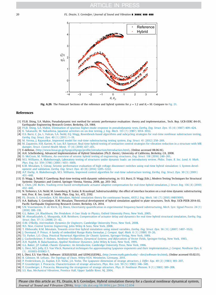
Fig. A.29. The Poincaré Sections of the reference and hybrid systems for μ = 1.2 and Ki¼10. Compare to Fig. 21.


References

[1] P.S.B. Shing, S.A. Mahin, Pseudodynamic test method for seismic performance evaluation: theory and implementation., Tech. Rep. UCB-EERC-84-01,Earthquake Engineering Research Center, Berkeley, CA, 1984.

[2] P.S.B. Shing, S.A. Mahin, Elimination of spurious higher-mode response in pseudodynamic tests, Earthq. Eng. Struct. Dyn. 15 (4) (1987) 409–424.[3] K. Takanashi, M. Nakashima, Japanese activities on on-line testing, J. Eng. Mech. 113 (7) (1987) 1014–1032.[4] O.S. Bursi, C. Jia, L. Vulcan, S.A. Neild, D.J. Wagg, Rosenbrock-based algorithms and subcycling strategies for real-time nonlinear substructure testing,

Earthq. Eng. Struct. Dyn. 40 (1) (2011) 1–19.[5] M. Verma, J. Rajasankar, Improved model for real-time substructuring testing system, Eng. Struct. 41 (2012) 258–269.[6] M. Zapateiro, H.R. Karimi, N. Luo, B.F. Spencer, Real-time hybrid testing of semiactive control strategies for vibration reduction in a structure with MR

damper, Struct. Control Health Monit. 17 (4) (2010) 427–451.[7] E-defense, ⟨http://www.bosai.go.jp/hyogo/ehyogo/profile/introduction/Introduction.html⟩, (Online accessed 08.06.16).[8] A.H. Schellenberg, Advanced Implementation of Hybrid Simulation (Ph.D. thesis), University of California, Berkeley, CA, 2008.[9] D. McCrum, M. Williams, An overview of seismic hybrid testing of engineering structures, Eng. Struct. 118 (2016) 240–261.

[10] M.S. Williams, A. Blakeborough, Laboratory testing of structures under dynamic loads: an introductory review, Philos. Trans. R. Soc. Lond. A: Math.Phys. Eng. Sci. 359 (1786) (2001) 1651–1669.

[11] K.M. Mosalam, S. Günay, Seismic performance evaluation of high voltage disconnect switches using real-time hybrid simulation: I. System devel-opment and validation, Earthq. Eng. Struct. Dyn. 43 (8) (2014) 1205–1222.

[12] A.P. Darby, A. Blakeborough, M.S. Williams, Improved control algorithm for real-time substructure testing, Earthq. Eng. Struct. Dyn. 30 (3) (2001)431–448.

[13] D. Wagg, S. Neild, P. Gawthrop, Real-time testing with dynamic substructuring, in: O.S. Bursi, D. Wagg (Eds.), Modern Testing Techniques for StructuralSystems: Dynamics and Control, Springer Vienna, Vienna, 2008, pp. 293–342.

[14] C. Chen, J.M. Ricles, Tracking error-based servohydraulic actuator adaptive compensation for real-time hybrid simulation, J. Struct. Eng. 136 (4) (2010)432–440.

[15] N. Terkovics, S.A. Neild, M. Lowenberg, R. Szalai, B. Krauskopf, Substructurability: the effect of interface location on a real-time dynamic substructuringtest, Proc. R. Soc. Lond. A: Math. Phys. Eng. Sci., 472, 2192.

[16] P.L. Drazin, S. Govindjee, K.M. Mosalam, Hybrid simulation theory for continuous beams, ASCE J. Eng. Mech. 141 (7) (2015) 04015005.[17] A.A. Bakhaty, S. Govindjee, K.M. Mosalam, Theoretical development of hybrid simulation applied to plate structures, Tech. Rep. UCB-PEER-2014-02,

Pacific Earthquake Engineering Research Center, Berkeley, CA, 2014.[18] S.N. Voormeeren, D. de Klerk, D.J. Rixen, Uncertainty quantification in experimental frequency based substructuring, Mech. Syst. Signal Process. 24 (1)

(2010) 106–118.[19] G.L. Baker, J.A. Blackburn, The Pendulum: A Case Study in Physics, Oxford University Press, New York, 2005.[20] M. Ahmadizadeh, G. Mosqueda, A.M. Reinhorn, Compensation of actuator delay and dynamics for real time hybrid structural simulation, Earthq. Eng.

Struct. Dyn. 37 (1) (2008) 21–42.[21] O.M. O'Reilly, Intermediate Dynamics for Engineers, Cambridge University Press, New York, 2008.[22] N.S. Nise, Control Systems Engineering, John Wiley & Sons, New York, 2008.[23] T. Elkhoraibi, K.M. Mosalam, Towards error-free hybrid simulation using mixed variables, Earthq. Eng. Struct. Dyn. 36 (11) (2007) 1497–1522.[24] J. Dormand, P. Prince, A family of embedded Runge-Kutta formulae, J. Comput. Appl. Math. 6 (1) (1980) 19–26.[25] T.S. Parker, L.O. Chua, Practical Numerical Algorithms for Chaotic Systems, Springer-Verlag, New York, 1989.[26] J. Guckenheimer, P. Holmes, Nonlinear Oscillations, Dynamical Systems, and Bifurcations of Vector Fields, Springer-Verlag, New York, 1983.[27] A.H. Nayfeh, B. Balachandran, Applied Nonlinear Dynamics, John Wiley & Sons, New York, 1995.[28] G.L. Baker, J.P. Gollub, Chaotic Dynamics: An Introduction, Cambridge University Press, New York, 1996.[29] L. Dieci, M.S. Jolly, E.S. Van Vleck, Numerical techniques for approximating Lyapunov exponents and their implementation, J. Comput. Nonlinear Dyn. 6

(1) . 011003-011003-7.[30] L. Dieci, E.S. Van Vleck, Software: LESLIS/LESLIL and LESNLS/LESNLL, ⟨http://www.math.gatech.edu/�dieci/software-les.html⟩, (Online accessed 03.02.15).[31] R. Gilmore, M. Lefranc, The Topology of Chaos, Wiley-VCH, Weinheim, Germany, 2011.[32] P. Frederickson, J.L. Kaplan, E.D. Yorke, J.A. Yorke, The Lyapunov dimension of strange attractors, J. Differ. Equ. 49 (2) (1983) 185–207.[33] P. Grassberger, I. Procaccia, Characterization of strange attractors, Phys. Rev. Lett. 50 (5) (1983) 346–349.[34] P. Grassberger, I. Procaccia, Measuring the strangeness of strange attractors, Phys. D: Nonlinear Phenom. 9 (1) (1983) 189–208.[35] S.S. Rao, Mechanical Vibrations, Prentice Hall, Upper Saddle River, NJ, 2004.


http://refhub.elsevier.com/S0022-460X(16)30793-3/sbref1












http://www.bosai.go.jp/hyogo/ehyogo/profile/introduction/Introduction.html





































http://www.math.gatech.edu/~dieci/software-les.html

http://www.math.gatech.edu/~dieci/software-les.html












Hybrid simulation theory for a classical nonlinear ...

Documents

Transcript of Hybrid simulation theory for a classical nonlinear ...