Modeling and Experimental Characterization of a Tethered

Spherical Aerostat

Philippe Coulombe-Pontbriand

Department of Mechanical Engineering

McGill University, Montreal, Canada

August 2005

A thesis submitted to McGill University, Montreal in partial

fulfillment of the requirements of the degree of

Masters of Science

Philippe Coulombe-Pontbriand, 2005

Abstract

Tethered helium balloons are known to be useful in applications where a payload

must be deployed at altitude for a long duration. Perhaps the simplest such system

is a helium-filled sphere tethered to the ground by a single cable. Despite its

relative simplicity, there exists little data about light tethered spheres in a fluid

stream. The current work focuses on an investigation of the dynamic

characteristics of a spherical aerostat on single tether. A test facility was

constructed to gather the experimental data required for a characterization of the

system. The balloon’s drag coefficient is extracted from the position

measurements. Our experiments were all in the supercritical range that is, at

Reynolds numbers greater than 3.7 × 105. We find that the balloon’s large

oscillations and surface roughness combined with the wind turbulence result in a

substantial increase in the drag coefficient. A model of the dynamics of a

spherical aerostat was previously developed at McGill University and our

experimental data was used to refine and improve that simulation. The aerostat is

modeled as a single body attached to the last node of a tether. It is subject to

buoyancy, aerodynamic drag and gravity. The tether is modeled using a lumped-

mass method. The dynamic simulation of the aerostat is obtained by setting up the

equations of motion in 3D space and integrating them numerically. Finally, the

model is validated through comparison with experimental data and a modal

analysis is performed.

ii

Résumé

Les ballons à hélium attachés au sol sont régulièrement utilisés lorsque des

charges doivent être déployées dans les airs pour une longue période. Le système

le plus simple consiste en un ballon sphérique attaché au sol par un seul câble.

Bien que ce système soit extrêmement simple, il n’existe que très peu

d’informations relatives aux sphères attachées dans un écoulement de fluide. Le

travail présenté dans cette thèse porte sur l’analyse de la dynamique d’un ballon

sphérique attaché au sol par un seul câble. La construction d’une installation

expérimentale a permis d’acquérir les données nécessaires à la caractérisation du

système. À partir des mesures de position, le coefficient de traînée du ballon a pu

être déduit. Toutes nos expériences ont été effectuées au delà du nombre critique

de Reynolds, i.e. supérieur à 3.7 × 105. Nous avons observé que les oscillations

du ballon ainsi que les imperfections de sa surface ont pour effet d’augmenter

considérablement le coefficient de traînée en comparaison avec un sphère fixe.

Nos données expérimentales ont été utilisées pour améliorer une simulation de la

dynamique du ballon développée à l’université McGill lors de recherches

antérieures. Le ballon est modélisé comme un corps rigide soumis à la gravité, à

la résistance de l’air et la force de poussée. La simulation est construite en

définissant les équations de mouvement du ballon en trois dimensions et en les

intégrant numériquement. Finalement, le modèle est validé en comparant les

résultats avec les données expérimentales.

iii

Acknowledgments

I would like to express my sincere gratitude to the people whose assistance and

support have allowed this research to be successful. First I want to thank my

supervisor Meyer Nahon for his constant guidance. You rarely meet someone who

inspires you for his human skills and research abilities. I would like to thank a

number of co-op students who brought fresh ideas and enthusiasm to this project.

These students are Domenico Mazzocca, Jennifer Perez and Magnus Nordenborg.

Thanks to my lab partners Jonathan Miller, Yuwen Li, François Deschênes and

Evgeni Kiriy for coming out to fly the balloons. A special thank to Casey Lambert

for his numerous advices and helping out with the experiment. Thanks to Alistair

Howard for biking with me.

Thanks to my brother Moïse for his support throughout the most difficult

years of my studies. I will never forget. Thanks to my loving sister Myriam who

inspired me courage and determination. I transmit a warm thanks to my parents,

Denis and Gilberte, for looking after me and reminding me that dreaming is

important, but more important still, is to live our dream.

Thanks to my friends, Dadou, Bast, Maestro, Regean (Big Monkey) et les

autres who are dancing and playing music tonight.

Finally, I want to express the warmest thanks to my girlfriend and life

partner Marleine Tremblay for being my life inspiration. Thank you for being

beside me day after day, thanks for allowing me to dream the world, thanks for

being who you are.

iv

Table of Contents

Abstract.................................................................................................................. ii Résumé .................................................................................................................. iii Acknowledgements .............................................................................................. iv Table of Contents .................................................................................................. v List of Figures...................................................................................................... vii List of Tables……………………………………………………………………..x 1. Introduction....................................................................................................... 1

1.1Overview........................................................................................................ 1 1.2 Motivation..................................................................................................... 2 1.3 Literature Survey .......................................................................................... 4

1.3.1 Tethered Aerostat Dynamics/Simulation............................................... 4 1.3.2 Sphere in Fluid Flow.............................................................................. 5

1.4 Thesis Contributions and Organisation......................................................... 6 2. Design of Test Facility ...................................................................................... 8

2.1 Requirements for the Experimental Set-Up.................................................. 8 2.2 Physical Platform .......................................................................................... 9

2.2.1 The Aerostat......................................................................................... 10 2.2.2 Tether ................................................................................................... 12 2.2.3 Winch................................................................................................... 15

2.3 Sensors and Communication Systems ........................................................ 15 2.3.1 GPS components .................................................................................. 16 2.3.2 Load Cell.............................................................................................. 18 2.3.3 SY016 A/D Board................................................................................ 18 2.3.4 Wind Sensors ....................................................................................... 19 2.3.5 Wireless Local Area Network (WLAN) .............................................. 21 2.3.6 Power ................................................................................................... 21 2.3.7 Summary .............................................................................................. 23

2.4 Software interface ....................................................................................... 23 2.5 The Instrument Platform ............................................................................. 24

2.5.1 Effect of the Platform on the Aerostat Properties ................................ 26 2.6. Experimental Procedure............................................................................. 27

3. Data Analysis ................................................................................................... 29 3.1 Days of experimentation ............................................................................. 29 3.2 Position ....................................................................................................... 30

3.2.1 Position Analysis ................................................................................. 30 3.3 Lift Force .................................................................................................... 34 3.4 Tension........................................................................................................ 35 3.5 Wind............................................................................................................ 37

3.5.1 Wind velocity, direction and frequency content .................................. 37

v

3.5.2 Power Law ........................................................................................... 39 3.5.3 Wind Extrapolation………………………………………………….. 40

3.6 Drag Force and Drag Coefficient................................................................ 41 3.6.1 Drag Force ........................................................................................... 41 3.6.2 Drag Coefficient................................................................................... 43

3.7 Aerostat Oscillations ................................................................................... 46 3.7.1 Axis Realignment................................................................................. 46 3.7.2 Oscillations .......................................................................................... 47 3.7.3 Scaling.................................................................................................. 49 3.7.4 Amplitude of Oscillation...................................................................... 50 3.7.5 Frequency of Oscillation...................................................................... 51 3.7.6 Nature of the Oscillations .................................................................... 53

4. Simulation of a Spherical Aerostat................................................................ 56 4.1 Original Model............................................................................................ 56

4.1.1 Cable Model......................................................................................... 57 4.1.2 Aerostat Model..................................................................................... 58 4.1.3 Wind Model ......................................................................................... 58

4.2 Proposed Model .......................................................................................... 59 4.2.1 Equations of Motion ............................................................................ 60 4.2.2 Revised Wind model…...……………………………………............ .65 4.2.3 Lateral Forces…………………………………………………………67

4.3 Physical Parameters .................................................................................... 69 4.3.1 Aerostat parameters ............................................................................. 69 4.3.2 Tether Parameters ................................................................................ 70

4.4 Non-linear Simulation Results and Comparison......................................... 71 4.5 Linear Model............................................................................................... 74

4.5.1 Description and Validation of the Linear Model ................................. 75 4.5.2 Decoupling........................................................................................... 77 4.5.3 Eigenvectors and Eigenvalues ............................................................. 78 4.5.4 Results.................................................................................................. 79 4.5.5 Reference Frequencies ......................................................................... 83

4.5.6 Damping Ratio..………………………………………………………86 5. Conclusion ....................................................................................................... 90

5.1 Test Facility .......................................................................................... 90 5.2 Data Analysis .............................................................................................. 91 5.3 Simulation ................................................................................................... 92 5.4 Recommendations....................................................................................... 94

References…...…………………………………………………………………..95

vi

List of Figures

Figure 1.1: Flight of the Montgolfier brother on June 1783[1] .............................. 1 Figure 1.2: Explosion of the Hindenburg on May 3, 1937[2] ................................ 2 Figure 1.3: Picture of a streamlined aerostat[3]...................................................... 3 Figure 2.1: Picture of the physical platform.. ......................................................... 9 Figure 2.2: Example of streamlined aerostat. The picture shows a TIF-460®

aerostat from Aerostar[36] ............................................................................ 10 Figure 2.3: Examples of variable lift aerostats. The balloon on the left is the

Skydoc® from FLOATOGRAPH[37] and the one on the right is the Helikite® from ALLSOPP[38]...................................................................................... 11

Figure 2.4: Technical drawing of the balloon showing the tether arrangement .. 14 Figure 2.5: Picture of the tether attachment configuration. A zoom on a strap used

to distribute the load is also shown ............................................................... 14 Figure 2.6: Picture of the CSW-1 winch supplied by A.G.O. Environmental

Electronics Ltd. ............................................................................................. 15 Figure 2.7: Diagram of the sensors/communication system. ................................ 16 Figure 2.8: Picture of the MLP75 load cell from Transducer Techniques. The two

eyebolt screws and carabiners were used to attached the cables at the confluence point............................................................................................ 18

Figure 2.9: Plot of the SY016 board calibration. The figure shows the highly linear response of the load system. ............................................................... 19

Figure 2.10: Picture of the wind tower with the Young wind sensors at 3, 5 and 10 m. ............................................................................................................. 19

Figure 2.11: Plots of the raw outputs of the Young anemometers. The top graph is the wind speed channel output. The middle graph is the excitation for the wind direction acquisition shown and the lower graph is the returned wind direction pulse. .............................................................................................. 20

Figure 2.12: Time variation of the voltage and current for a continuous acquisition. The tension acquisition failed after 6.5 hours. .......................... 22

Figure 2.13: Information flow of the software interface....................................... 24 Figure 2.14: On the left is a Pro-E drawing of the platform. The picture on the

right shows how the platform was attached to the balloon........................... 25 Figure 2.15: The left picture shows a technical drawing of the platform that with the four stabilization lines. On the right is a picture of the actual platform.......... 26 Figure 2.16: The ground handling of the balloon was perfromed by one person. A

soft carpet was used to keep the balloon close to the ground. ...................... 28 Figure 3.1: Schematic of the relative positions of the components of the aerostat system. .................................................................................................................. 31 Figure 3.2: Magnitude of rWA for Flight 9. ........................................................... 32

vii

Figure 3.3: Components of rWA for Flight 9.......................................................... 32 Figure 3.4: Schematic of the variable relevant to the calculation of the mean

angle. ............................................................................................................. 33 Figure 3.5: Time history of the angle for Flight 9. ............................................... 34 Figure 3.6: Plot of the free lift measured with the Transducer Techniques load cell

....................................................................................................................... 35 Figure 3.7: Plot of the tension data for Flight 9, compared to the aerostat free lift

line................................................................................................................. 36 Figure 3.8: Tether tension at the different cable lengths. ..................................... 36 Figure 3.9: Graph of the wind speed and direction at 3, 5 and 10 metre for Flight

9..................................................................................................................... 37 Figure 3.10: Power spectrum of the wind of Flight 9 at 10m height. ................... 38 Figure 3.11: Plot of the average wind speed against the height for Flight 9. A power law is fitted to extract the value of the exponent…………………………39 Figure 3.12: Plot of the fitted wind speed of Flight 9. The wind speed at 3m is

shown to show how the 10th order polynomial smoothes the curve. ............ 41 Figure 3.13: Ideal sketch of the aerostat equivalent static system. ....................... 42 Figure 3.14: This figure shows the drag force versus the wind speed. A curve is

fitted to demonstrate the quadratic dependence on the velocity. .................. 43 Figure 3.15: Comparison of the sphere drag coefficients ..................................... 45 Figure 3.16: Top view of the aerostat to show the new coordinate frame aligned

with the wind direction ................................................................................. 46 Figure 3.17: Typical projection trajectory in the horizontal plane ....................... 48 Figure 3.18: Oscillatory behaviour of the aerostat for Flight 9.. .......................... 48 Figure 3.19: Comparison of the normalized oscillation amplitude of the tethered

sphere used in experiment with the Govardhan and Williamson results. ..... 51 Figure 3.20: Power spectrum of the transverse motion for Flight 9 ..................... 52 Figure 4.1: 2-D sketch of the original model showing the discretization of cable.

....................................................................................................................... 57 Figure 4.2: Cable element and node representation.............................................. 58 Figure 4.3: Idealized sketch of the proposed aerostat model. rT is the vector from

centre of gravity to the confluence point and FT is the resultant force of the last element acting on the aerostat. ............................................................... 59

Figure 4.4: Idealized sketch of the aerostat system showing the body-fixed and inertial frames. .............................................................................................. 60

Figure 4.5: Free body diagram of a tethered sphere in a fluid flow...................... 61 Figure 4.6: Comparison of the turbulent intensities vs. height from various

sources. A zoom on heights below 50 m is presented to better show the region of interest. .......................................................................................... 66

Figure 4.7: The power spectral density for the measured and simulated horizontal turbulence along the wind direction for Flight 9 and Flight 4. ..................... 67

Figure 4.8: Comparison of experimental and simulated results for the aerostat position for Flight 9 at L=15m...................................................................... 74

Figure 4.9: Comparison of the experimental and simulated results for the tether tension for Flight 9 at L=15m ....................................................................... 74

viii

Figure 4.10:Comparison of the linear and non-linear response of the aerostat motion for a tether length L=45 m and wind speed U =1 m/s ..................... 77

Figure 4.11: Magnitude of the response of the different state variables fo the lowest 4 longitudinal modes. ........................................................................ 80

Figure 4.12: Graphical representation of the various modes of oscillation of a spherical tethered aerostat............................................................................. 82

Figure 4.13: Spectral density of the tension for Flight 9 for the various tether lengths. The black spike shows the values of the theoretical frequencies. ........... 86 Figure 4.14: The schematic on the left shows a free body diagram of a pure x-

motion of the aerostat.................................................................................... 86

ix

List of Tables

Table 2.1 Comparison of streamlined and spherical aerostat properties[33]........ 11 Table 2.2: Comparison of the properties of the Plasma® rope from Cortland

cable[37] and of a simple Nylon Cable......................................................... 13 Table 2.3 System Components ............................................................................. 23 Table 2.4: Total load on the aerostat..................................................................... 25 Table 2.5: Comparison of the Physical Properties of the Aerostat and a Spherical

Shell filled with helium................................................................................. 27 Table 3.1 Wind condition for the different days of experimentation.................... 30 Table 3.2: Position data of Flight 9....................................................................... 33 Table 3.3: Mean tension at the different cable lengths for Flight 9 ...................... 37 Table 3.4: Wind characteristics of Flight 9........................................................... 38 Table 3.5: List of parameters of interest for the calculation of the drag coefficient

CD .................................................................................................................. 44 Table 3.6: Position data of Flight 9 after realignment .......................................... 47 Table 3.7: Comparison of the dimensionless quantities for the aerostat used in

this experiment and the Williamson’s tethered sphere. ................................ 50 Table 3.8: Comparison of the dominant frequency in power spectrum with the

theoretical pendulum frequency of the system for Flight 9 .......................... 52 Table 4.1: Physical parameters ............................................................................. 70 Table 4.2: Tether parameters ................................................................................ 71 Table 4.3: Comparison of experimental and simulated results for the three flight

sections of Flight 9........................................................................................ 72 Table 4.4: Comparison of the analytical and model modal frequencies for L =

45m ............................................................................................................... 84 Table 4.5: Comparison of the simulated and theoretical damping ratio for U=1m/s

and L=45m.................................................................................................... 88

x

Pour ma mère Cécile

xi

Chapter 1

Introduction

1.1 Overview

The Montgolfier brothers, born in Annonay, France, are the inventors of the first practical

balloon for flight. The first demonstrated flight of a hot air balloon took place on June 4,

1783, in Annonay, France in front of an astonished crowd.

Figure 1.1: Flight of the Montgolfier brothers on June 1783[1].

Less than six months after the ground-breaking Montgolfier flight, the French physicist

Jacques Charles (1746-1823) and Nicolas Robert (1758-1820) made the first untethered

ascension with a hydrogen filled balloon on December 1, 1783. On that same day was

born a completely new research area, the study of lighter-than-air systems. These types of

systems include any vehicle capable of deriving its lift from the buoyancy of its internal

gasses rather than from its aerodynamics. The golden age of lighter-than-air systems

1

happened during the beginning of the 20th century with the advent of the Zeppelin

airships. These were gigantic rigid dirigibles filled with hydrogen to transport civilians

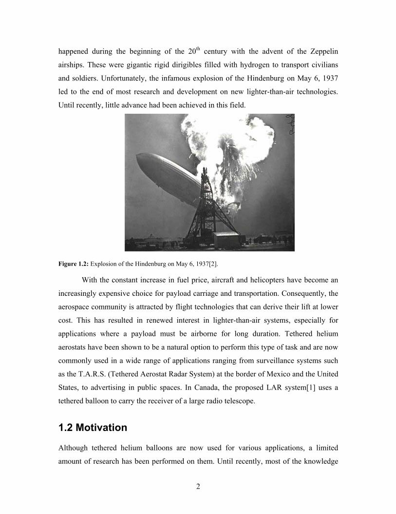
and soldiers. Unfortunately, the infamous explosion of the Hindenburg on May 6, 1937

led to the end of most research and development on new lighter-than-air technologies.

Until recently, little advance had been achieved in this field.

Figure 1.2: Explosion of the Hindenburg on May 6, 1937[2].

With the constant increase in fuel price, aircraft and helicopters have become an

increasingly expensive choice for payload carriage and transportation. Consequently, the

aerospace community is attracted by flight technologies that can derive their lift at lower

cost. This has resulted in renewed interest in lighter-than-air systems, especially for

applications where a payload must be airborne for long duration. Tethered helium

aerostats have been shown to be a natural option to perform this type of task and are now

commonly used in a wide range of applications ranging from surveillance systems such

as the T.A.R.S. (Tethered Aerostat Radar System) at the border of Mexico and the United

States, to advertising in public spaces. In Canada, the proposed LAR system[1] uses a

tethered balloon to carry the receiver of a large radio telescope.

1.2 Motivation

Although tethered helium balloons are now used for various applications, a limited

amount of research has been performed on them. Until recently, most of the knowledge

2

of these systems was based on experiments and qualitative research. Some understanding

of their behaviour was attained, but very little was known about the forces and moments

acting on balloons in flight. With the advent of new technologies and the increasing

desire to use tethered aerostats in advanced applications where reliability is critical,

systematic studies of the system stability and nonlinear simulation have become more

important to better understand the system behaviour. This understanding comprises a

challenge that can only be resolved using a multidisciplinary perspective including

system dynamics, fluid-structure interaction, simulation and meteorology. Questions such

as how a tethered balloon would react in strong turbulent winds are still to be answered

and the tools to answer it are yet to be developed and integrated.

Most of the past research has been performed on so-called streamlined or blimp

shaped balloons as shown in Figure 1.3.

Figure 1.3: Picture of a streamlined aerostat[3].

This appears to be a natural choice since they present advantages for flight such as low

aerodynamic drag and the ability to produce aerodynamic lift. However, with the desire

to apply lighter than air technology in innovative applications such as payload carriage,

fast deployment surveillance systems, or even low cost aerial photography, some new

variables have to be taken into account like the stability of the system in winds and ease

of deployment and use. New balloon shapes might be more suitable for these

applications, but there exists very little research in the open literature in this field. A

3

natural candidate to study is the spherical shape tethered helium aerostat which presents

the advantage of having no preferred orientation with respect to the wind, being relatively

easy and fast to build and having the most efficient volume to free lift ratio (due to its low

surface area). Surprisingly enough, although a spherical object attached to the ground by

a single tether in a flow is one of the simplest engineering systems one can think of, there

exists little data about it in the open literature.

1.3 Literature Survey

This thesis spans many different subjects in the literature from meteorology for wind

characterization to balloon design. However the main subject of interest is the study and

simulation of the dynamics of a tethered spherical aerostat in a wind field. This requires

an accurate knowledge of past research done on the simulation of aerostats and on the

interaction of a sphere with a fluid flow.

1.3.1 Tethered Aerostat Dynamics/Simulation

Tethered aerostats have received limited attention in the literature and most of the focus

has been directed at large streamlined aerostat. The study of the dynamics of a spherical

aerostat in wind and its simulation is still an almost untouched subject. One exception is

the work of Lambert[4], who performed a preliminary simulation of the dynamics of a

spherical tethered aerostat in a fluid flow, without experimental validation. Furthermore,

to the author’s knowledge, no data about tethered spherical aerostat motion in wind fields

has been published. The simulation of tethered streamlined aerostats has greatly

influenced this work and includes the work of Delaurier in 1972, who was the first to

study the dynamics of a tethered aerostat with a comprehensive cable model[5]. In 1973,

Redd et al., used experimental data to validate their linear simulation[6]. Jones and

Krausman in 1982 completed the first 3-D nonlinear dynamics model with a lumped

mass discretized tether[7]. Jones and Delaurier further developed this concept to come up

with a model based on semi-empirical values[8]. In 1999, Nahon presented a 3-D

nonlinear method to study a tri-tethered spherical aerostat in a wind field using a lumped

mass cable model[9]. The method was based on prior work performed on autonomous

underwater vehicles[10], submerged cable[11] and towed underwater vehicle[12]. More

4

recently, in 2001 Jones and Schroeder, performed a validation of their nonlinear model

using results from full scale flights test of an instrumented tethered aerostat[13] provided

by the U.S. army. In 2003, Lambert and Nahon presented a nonlinear model of a tethered

streamlined aerostat and suggested a method to assess the stability of a single tethered

aerostat by linearization of the equations of motion[14]. The response of the streamlined

tethered aerostat to extreme turbulence was studied by Stanney and Rahn who used a

sophisticated wind model[15]. Lambert in 2005[16] used the results from experiments

performed on a fully instrumented 20 m long tethered streamlined aerostat that was

deployed in the scope of the LAR[17] project to perform a validation of its nonlinear

model.

1.3.2 Sphere in Fluid Flow

The interaction of fixed sphere with a fluid flow and the wake that results behind it are

encountered so frequently that large numbers of experiments have been conducted and an

enormous amount of data has been accumulated. An excellent summary of the

characteristics of vortex shedding of a fixed sphere in fluid flow over a wide range of

Reynolds number is presented by Sakamoto and Haniu[18]. They divided the vortex

shedding into three regimes based on Reynolds number and vortex structure. Below a

Reynolds number of 300, there is no vortex shedding; between 300 and 2×104 the vortex

shedding is periodic and finally, above 2×104 there is strong vortex shedding although not

periodic. At a critical value of the Reynolds number, the previously laminar boundary

layer becomes turbulent. This corresponds with a sudden drop in the drag because of a

decrease in the size of the wake. Achenbach[19] in 1972 and Tenada in 1977[20]

described in detail the shape and characteristics of the wake of a fixed sphere at very high

Reynolds number (above 3.5×105), past the supercritical regime of flow where the

present experiment is performed. Willmarth and Enlow in 1969 measured for the first

time the unsteady lateral lift force generated by the vortex shedding acting on the fixed

sphere in the supercritical regime and provided a detailed study of its magnitude and

frequency content[21]. Thirty years later, Howe et al.,[22] performed measurement of the

lift force on a fixed sphere for a similar flow regime that were in agreement with

Willmarth and Enlow. They also discussed the possible contribution of the lift force to

5

the erratic motion of rising spherical weather balloon discussed by Scoggins in 1967[23,

24].

To the author’s knowledge the first reported study of the oscillation of tethered

spheres in a fluid flow was performed in Moscow university by Kruchinin[25]. He

attributed the oscillation of the tethered sphere to its acceleration, which created a surface

pressure unbalance at the critical Reynolds number. Other studies in the literature are

concerned with the action of surface waves on a tethered buoyant spherical structure.

These include the work by Harleman and Shapiro in 1961[26], Shi-Igai and Kono

1969[27] and Ogihara in 1980[28]. They employed empirically determined drag and

inertia coefficient to predict the sphere dynamics. The first group to give systematic

attention to the transverse oscillations of tethered sphere in a fluid flow was Govardhan

and Williamson and Williamson and Govardhan 1997[29] [30]. In 2001, Jauvtis et al.,

explained the sphere oscillations by a ‘lock in’ phenomenon of the principal vortex

shedding as described for a fixed sphere and the body motion[31]. They also discovered

the existence of a mode of oscillation at much higher flow speeds that could not be

explained by the classical ‘lock in’ theory since the vortex shedding of the fixed sphere in

that flow regime would have no frequency content close to the natural pendulum

frequency of the tethered sphere. Govardhan and Williamson provided the explanation to

the unexpected phenomenon in 2005[32]. They attributed the oscillations of the tethered

sphere to ‘movement induced vibration’ as categorized by Naudasher and Rockwell in

1994[33] where the sphere motion generates self-sustaining vortex forces. Other research

in that field includes the work of Bearman in 1984[34] and Anagnostopoulos in 2002[35].

1.4 Thesis Contributions and Organisation

The focus of the present work is the analysis and simulation of the dynamics of a tethered

spherical aerostat in a wind field. This includes the design and construction of an

experimental platform capable of recording the tether forces and the motion of the

aerostat; the analysis of the motion data; and a computer simulation of the aerostat

behaviour.

In Chapter 2, a detailed description of the experimental platform is presented. It

discusses a method to accurately measure the time history of the aerostat position and of

6

the tether tension. A rationale for the choice of sensors, tether, aerostat size and other

physical components is provided. The chapter ends with a discussion of the experimental

procedure.

Chapter 3 presents a detailed examination of the dynamics of the 3.5 m diameter

spherical aerostat used in the experiment. A method to extract the average drag

coefficient of the tethered buoyant sphere in an outdoor environment is presented. The

experimental motion data present clear perpendicular to flow oscillations of the aerostat.

A characterization of the aerostat’s large transverse vibration is presented and various

potential explanations for the phenomenon are explored.

In Chapter 4, the dynamics model developed by Lambert[4] for a spherical

aerostat is used as basis to generate a more detailed and accurate model. A brief

introduction to the dynamics model by Lambert is presented first. This is followed by

details of the modifications made to the original model to make it more representative of

the tethered aerostat system used in the experiment. The results of the nonlinear model

are then compared to experimental data and conclusions are drawn. Finally, the dynamics

model is used to conduct a linear analysis of the system. The equations of motion are

linearized about an equilibrium state and a thorough modal analysis is performed.

Chapter 5 presents the conclusions of the research as well as recommendations for

future work.

7

Chapter 2

Design of Test Facility

In this chapter, the construction and operation of a portable experimental set-up for the

characterization of the dynamics of a tethered aerostat are presented. The experimental

set-up is divided into four subsystems, the physical platform, the sensor system, the

communication system and the software interface. Section 2.1 discusses the performance

requirements used to guide the design of the set-up. Section 2.2 describes the design of

the system, which includes the balloon, the tether, the winch and the instrument platform.

In Section 2.3, descriptions of the sensors and of the communication system are

presented. The different options considered for the communication system are compared.

Section 2.4 gives a description of the interfacing software DATAS (Dynamics

Acquisition of a Tethered Aerostat System), an in-house software for sensor integration

and time synchronization. In Section 2.5 a description of the platform that carries the

airborne instrumentations is given. Finally, Section 2.6 describes the experimental

procedure, including the process from ground handling to launching.

2.1 Requirements for the Experimental Set-Up

Prior to giving a detailed description of the experimental set-up, it is important to

describe the goals and performance requirements of the facility. The ultimate goal was to

develop a light and compact experimental set-up that would allow accurate measurement

of the time history of the balloon’s motion and of the tension in the cable. These two

variables are sufficient to fully describe the dynamics of the system; to extract all the

forces acting on the aerostat. The design of the facility was adopted based on the

following requirements:

8

The sensors should provide centimetre level accuracy on position measurement,

and frequency bandwidth of 2.5 Hz both on the position and tension acquisitions.

The aerostat free lift (net upward force) should be at least 12 kg without the

instruments onboard.

The total weight of the instrumentation carried by the balloon should be as low as

possible.

The entire set-up should be compact and convenient to use. It should not require

more than 2 people to operate safely.

A single experiment should not take more than 5 hours to perform.

The facility should accommodate different shapes of aerostat.

The sensing system should have a minimal impact on the natural dynamics of the

system.

The system should withstand gusts of up to 15 m/s and operating wind speed of

10 m/s.

2.2 Physical Platform

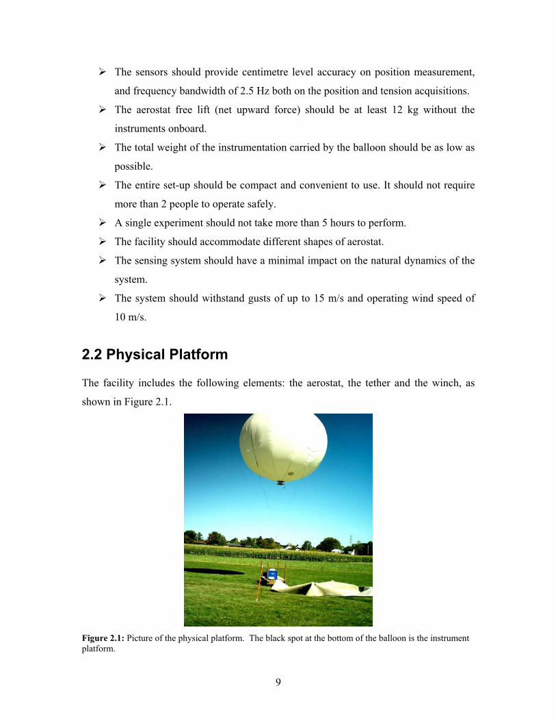
The facility includes the following elements: the aerostat, the tether and the winch, as

shown in Figure 2.1.

Figure 2.1: Picture of the physical platform. The black spot at the bottom of the balloon is the instrument platform.

9

2.2.1 The Aerostat

The main factors that influence the choice of a particular aerostat are its shape, its size, its

survivability its cost and its availability.

The two most popular shapes of aerostats available on the market are the

streamlined and the spherical aerostat. Figure 2.2 shows a picture of the TIF-460®, a

streamlined aerostat manufactured by Aerostar. An example of a spherical aerostat is

shown in Figure 2.1.

Figure 2.2: Example of streamlined aerostat. The picture shows a TIF-460® aerostat from Aerostar[36].

Other shapes of aerostat that provide variable lift are available but are quite uncommon.

Figure 2.3 shows two examples of this kind of aerostat, the Skydoc® from

FLOATOGRAPH technologies and the Helikite® from ALLSOPP.

10

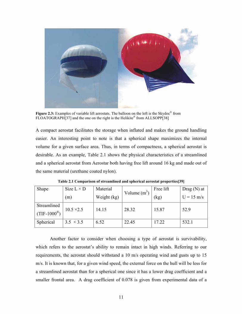
Figure 2.3: Examples of variable lift aerostats. The balloon on the left is the Skydoc® from FLOATOGRAPH[37] and the one on the right is the Helikite® from ALLSOPP[38]

A compact aerostat facilitates the storage when inflated and makes the ground handling

easier. An interesting point to note is that a spherical shape maximizes the internal

volume for a given surface area. Thus, in terms of compactness, a spherical aerostat is

desirable. As an example, Table 2.1 shows the physical characteristics of a streamlined

and a spherical aerostat from Aerostar both having free lift around 16 kg and made out of

the same material (urethane coated nylon).

Table 2.1 Comparison of streamlined and spherical aerostat properties[39]

Shape Size L × D

(m)

Material

Weight (kg) Volume (m3)

Free lift

(kg)

Drag (N) at

U = 15 m/s

Streamlined

(TIF-1000®) 10.5 ×2.5 14.15 28.32 15.87 52.9

Spherical 3.5 × 3.5 6.52 22.45 17.22 532.1

Another factor to consider when choosing a type of aerostat is survivability,

which refers to the aerostat’s ability to remain intact in high winds. Referring to our

requirements, the aerostat should withstand a 10 m/s operating wind and gusts up to 15

m/s. It is known that, for a given wind speed, the external force on the hull will be less for

a streamlined aerostat than for a spherical one since it has a lower drag coefficient and a

smaller frontal area. A drag coefficient of 0.078 is given from experimental data of a

11

streamlined body in McCormick[40]. The drag coefficient of the sphere was estimated

based on values for rough fixed sphere. Goldstein[41] mentions that the surface

roughness considerably reduces the supercritical drop in drag coefficient that normally

occurs around a Reynolds number of 3.7×105 [42], leading to an almost constant

coefficient. Thus the value of drag coefficient was estimated to 0.4, which corresponds

to that of a fixed sphere in the subcritical region[42]. A better estimate of the drag

coefficient will be obtained in Chapter 4. The drag force is expressed as

Da ACUD 2

21 ρ= (2.1)

where CD is the drag coefficient, aρ is the air density taken as 1.229 kg/m3, U the free

stream velocity and A is the sphere’s frontal area, πr2, where r is equal to 1.75 m for the

spherical balloon and 1.25 for the streamlined one. As seen in Table 2.1, the estimated

drag force for U = 15 m/s on a spherical aerostat with 16 kg lift is about eight times larger

than for a streamlined balloon with similar lift. However, balloons that withstand our

operating conditions are available on the market in both shapes. In terms of cost,

streamlined aerostats are more expensive than spherical ones. Normally, a streamlined

aerostat will cost 30 to 50 percent more for the same free lift.

A decision was made to use a 3.5 m spherical aerostat made out of urethane

coated nylon to keep the system as small a possible. Also, from a scientific perspective,

the experimental characterization of the dynamics of a spherical tethered body in

turbulent flow is of prime interest since there is little data available on the subject even

though such systems are commonly used. The balloon was bought from Aerostar, due to

their professional approach at answering our numerous questions, and their interest in

collaboration.

2.2.2 Tether

The choice of tether material was made based on expertise developed at McGill in the

context of the LAR project [17]. That system has successfully used Plasma® rope from

Cortland Cable to tether their streamlined aerostat to the ground. This particular material

is characterized by a very high elastic modulus and strength to weight ratio. It is clear that

12

lighter tethers are desirable since a heavy cable would reduce the lift available to carry

the instrumentation.

In order to determine the required cable diameter, an estimate was made of the

static tension for a wind of 15 m/s. Assuming an equilibrium of forces acting on the

balloon between the free lift L, the cable tension T and the aerodynamic drag D, we can

solve for T using

22 LDT += (2.2)

where D is calculated using equation (2.1) and equals to 532.1 N at 15 m/s. For these

calculations, the lift was taken to be 168.8 N, thus yielding a tension of 558.2 N. In a real

environment, the acceleration of the balloon would contribute to increase the maximum

tension. For that reason, a factor of safety of at least three should be respected on the

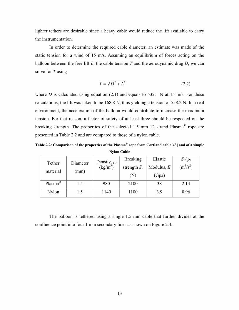
breaking strength. The properties of the selected 1.5 mm 12 strand Plasma® rope are

presented in Table 2.2 and are compared to those of a nylon cable.

Table 2.2: Comparison of the properties of the Plasma® rope from Cortland cable[43] and of a simple

Nylon Cable

Tether

material

Diameter

(mm)

Density, ρt (kg/m3)

Breaking

strength Sb

(N)

Elastic

Modulus, E

(Gpa)

Sb/ ρt

(m4/s2)

Plasma® 1.5 980 2100 38 2.14

Nylon 1.5 1140 1100 3.9 0.96

The balloon is tethered using a single 1.5 mm cable that further divides at the

confluence point into four 1 mm secondary lines as shown on Figure 2.4.

13

Figure 2.4 Technical drawing of the balloon showing the tether arrangement.

Using multiple secondary lines contributes to reducing stress on the aerostat

fabric at the attachment. To further distribute the stress on the fabric, two straps were

sewn along the surface of the balloon, each starting from one of the secondary lines, over

the top of the balloon, ending at the opposing secondary line. The four secondary lines

were attached to these straps as shown on Figure 2.5.

Figure 2.5: Picture of the tether attachment configuration. A zoom on a strap used to distribute the load is also shown

14

2.2.3 Winch

Winch selection was inspired by previous research in the scope of the LAR project. The

CSW-1 model, shown in Figure 2.6, was purchased from A.G.O. Environmental

Electronics Ltd .

Figure 2.6: Picture of the CSW-1 winch supplied by A.G.O. Environmental Electronics Ltd.

The main advantages of the CSW-1 winch are that it is compact and is battery powered.

These features are desirable since it allows flexibility in the choice of launch site. The

winch weighs 30 Kg and has outer dimensions of 63.5 × 55.9 × 45.7 cm (L×W×H). A

standard permanent magnet, face mount Leeson motor (model M1120046) drives the

winch. The motor rating is 124 Watts at 12 VDC for a typical current load of about 10 A.

The winch is powered by a standard 12 V lead/acid car battery and can retrieve a 30 kg

load at a rate of 6-10 m/min. The motor speed reducer system consists of a gearbox and a

sprocket drive. The gearbox has a 30:1 ratio and the sprocket drive 1:2.5 for an

equivalent gearing of 12:1. The winch is manually controlled through a control box with

buttons for forward and reverse operation. The winch is equipped with a manual brake

and manual crank drive in case of emergency. To facilitate its transportation, it was

bolted to a wheeled platform.

2.3 Sensors and Communication Systems

The sensors and communication systems are used to collect experimental data for the

characterization of the aerostat dynamics. The systems must be able to accurately

measure the environmental conditions as well as the aerostat response without altering

15

the natural behaviour of the aerostat. Different options were considered by David

Aristizabal, a work-term student. The final sensors and communication system can be

divided into two subsystems: the ground-based components, which enable ground

handling and operation, and the airborne components flying with the aerostat. All the

components are shown in Figure 2.7. These components are now considered in more

detail.

Figure 2.7: Diagram of the sensors/communication system

2.3.1 GPS components

The choice of GPS system was based upon compactness and accuracy. A minimal

accuracy of 5 cm on the position was required in order to describe the motion of the

16

aerostat precisely. One of the only commercially available technology that can achieve

this accuracy over long distances is differential GPS or DGPS[44]. The underlying

premise of DGPS requires that a GPS receiver, known as the base station, be set up at a

precisely known location. The base station receiver calculates its position based on

satellite signals and compares this location to the known location. The corrections thus

obtained can then be applied to the GPS data recorded by the roving GPS receiver located

on at the aerostat.

The DGPS hardware was purchased from NovAtel a Calgary based company and

consists of two GPS receivers and two antennas. The base receiver is the DL-4 plus. It is

powered by an OEM4-G2L card which is L1/L2 carrier phase compatible. The DL-4 plus

features 2 RS-232 ports with speeds up to 230,400 bits per second. One of the ports is

used for data collection while the other is used for time synchronisation of the different

sensors. This GPS unit can achieve an accuracy of 1.5 m on position before differential

correction at a rate of 20 Hz. The enclosure size is 185×154×71 mm and it weighs 1200

g. Nominal power consumption is 3.5 W with an input voltage of 9-18 VDC. The base

receiver antenna model is the GPS-702. It is also compatible with L1/L2 carrier phase

measurements and designed for very high accuracy measurement.

For its part, the rover receiver/antenna system has to be low power, compact, very

accurate, and most of all very light. For that purpose a FlexPak receiver and a GPS-512

antenna from NovAtel were used. The FlexPak receiver offers L1/L2 compatibility and

offers two RS-232 output ports. The main characteristics and operation of the rover

receiver are identical to the base receiver except for its compact size 147×123×45 mm, its

low weight, 307 g, and its low power consumption, 2.6 W, with an input voltage of 6-18

VDC. The GPS-512 antenna is also L1/L2 compatible. It measures 76×119× 19 mm and

weighs only 0.198 kg. The bandwidth of the GPS-512 is slightly less than that of the

GPS-702 and the noise level a little higher.

A post-processing DGPS software called GrafNav was purchased from Waypoint

Consulting Inc. GrafNav has the capability to post-process kinematic baseline to cm level

accuracy and static baseline to sub-millimetre accuracy. It also uses Kalman filtering to

fix otherwise unrecoverable cycle slips. With this software, an accuracy of about 5 cm

was achieved on the position. The software package also comes with a GPS data logger,

17

which was used to log the rover and receiver GPS position directly into ‘.gpb’ files, the

native GrafNav format.

2.3.2 Load Cell

To meet our load requirement, an MLP75 load cell from Transducer Techniques was

selected. This lightweight and compact unit can measure loads up to 75 pounds with a

safe overload of 150%. Its size is 41.66×19.05×12.7 mm and it weighs 70 g. The rated

output is 2 mV/V and the excitation voltage is 5 VDC. The temperature compensation

goes from 15.5 to 71°C with a maximum effect of 0.005% on the output. Tension in the

main tether was measured by placing the cell directly at the confluence point using two

eye-bolt screws and two karabiners as shown in Figure 2.8.

Figure 2.8: Picture of the MLP75 load cell from Transducer Techniques. The two eyebolt screws and karabiners were used to attach the cables at the confluence point

2.3.3 SY016 A/D Board

The load cell analog signal was digitized to RS-232 using a SY016 digital conditioner

and amplifier from Synectic Design. It was enclosed in an aluminium box measuring

62×43×33 mm for a total weight of 90 g. The board consumes on average 0.6 W with an

input voltage of 10-12 VDC and provides a 5 V bridge excitation. It can send up to 400

readings/sec. with a baud rate of 2400-115 200 bits/sec.

The board was calibrated in the laboratory by applying known loads to the cell

and recording the output at 10 hertz for periods of 30 seconds at each different load. The

18

data was then averaged over each 30 seconds plateau. From these measurements, a linear

plot of the load versus the amplifier output was determined as shown in Figure 2.9.

Figure 2.9: Plot of the SY016 board calibration. The figure shows the highly linear response of the load system.

The equation of the interpolated curve is used to convert the SY016 board readings into

Newtons during post-processing.

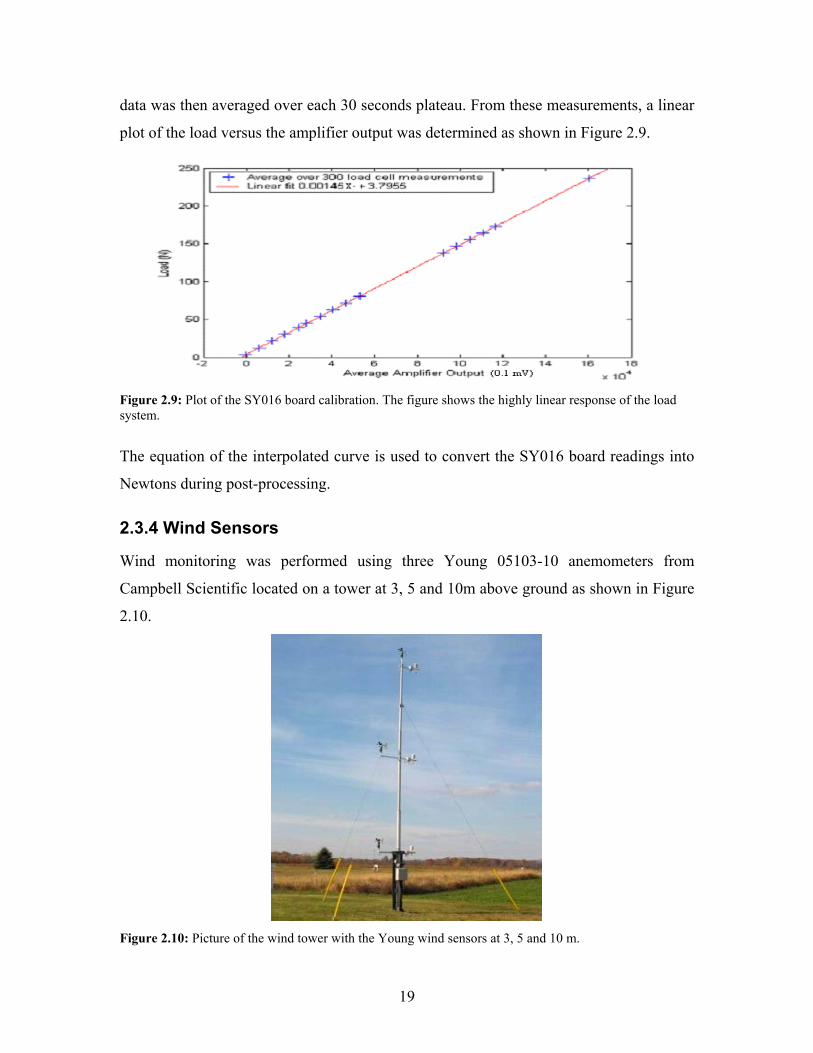
2.3.4 Wind Sensors

Wind monitoring was performed using three Young 05103-10 anemometers from

Campbell Scientific located on a tower at 3, 5 and 10m above ground as shown in Figure

2.10.

Figure 2.10: Picture of the wind tower with the Young wind sensors at 3, 5 and 10 m.

19

Each sensor records the wind speed and the wind direction relative to the true north. The

raw voltage signals from the sensors were sampled and stored at 300 hertz using a PMD-

1208FS digitizer from Measurement Computing. For that purpose, six channels of the

digitizer were used, one recording the wind speed and one recording the wind direction

for each sensor. Figure 2.11 presents the shape of typical raw output signals from a

Young anemometer. The top plot is the sinusoidal wind speed voltage, the middle plot is

the returned wind direction pulse, and the lower plot is the excitation signal that triggers

the wind direction pulse.

Figure 2.11: Plots of the raw outputs of the Young anemometers. The top graph is the wind speed channel output. The middle graph is the returned wind direction pulse and the lower graph is the excitation for the wind direction acquisition.

The wind acquisition is post-processed using the DATAS software (to be discussed in

Section 2.4). The frequency of the sinusoidal output voltage is converted using the

following equation [45]:

0.098U f= (2.3)

where U is the wind speed in m/s and f is the number of cycles per second. The frequency

f of the sinusoidal wave was obtained during post-processing by counting the number of

cycles over each 0.2 second period of acquisition thus, leading to a wind speed

acquisition rate of 5 Hz.

The wind direction sensor had a 5 degrees deadband between 355º and 360º, and

it is given by 3552.5 W where 2.5 is the excitation voltage amplitude and W is the returned

wind direction voltage. The wind direction sensors have been calibrated so that the zero

20

volt output occurs when the wind blows from true north, and voltage increases as the

wind direction increases clockwise. The acquisition rate on the wind direction is limited

by the 0.5 Hz excitation rate over which we had no control.

2.3.5 Wireless Local Area Network (WLAN)

Although a slip ring was available on the winch to allow transmission of data and power

through the tether, the line length was greater than could be accommodated by the RS-

232 protocol used by the GPS unit. Wireless communication was therefore used. For our

system, the GPS is the most demanding sensor. Each position log is 4640 bits long and

thus, to log the position at 10 Hz, an effective baud rate of at least 46400 is required. The

tension log is only 176 bits long, thus requiring an additional baud rate of 1760.

A WLAN was assembled to transmit the roving GPS and the tension data to

ground. It consists of a DataHunter dual RS-232 SeriaLan and a D-Link DI-614 802.11g

wireless router used as an access point (refer to Figure 2.7). The outer casing of the

SeriaLan measures 116×88×27 mm and its total weight is 310 g. In normal operating

condition, the DataHunter consumes 3 W with 5-15 VDC input. It features two RS-232

ports that can be configured from 300 to 115200 baud rate. The roving GPS uses one of

the ports and the load cell digital amplifier the other. The data is transmitted to the D-

Link router via a radio link and then to the PC via the Ethernet port. The data stream is

finally converted back into RS-232 format using TCPCOM, a software by TAL

Technologies that creates two virtual COM ports on the computer.

The SeriaLan ports were set to 115200 baud rate since 56200 is too close to the

data transmission requirement. In order to determine the effective baud rate of the

system, a stream of 10 kilobytes was sent to the LAN and retransferred to PC via the

virtual RS-232 wireless connection. The effective baud rate was determined to be about

93000 when the base station was located 100 meters from the instrument platform. Since

the aerostat does not fly above 45 m, the WLAN set-up meets our requirements.

2.3.6 Power

Two options were considered: onboard batteries and power transmitted from the ground

through the winch and tether. The onboard battery system led to a lower system weight

(batteries are lighter than copper wires) and was therefore chosen.

21

A typical experiment takes about 2 hours to perform, and it is desirable to have

the batteries last for at least three experiments. Thus the batteries are required to last at

least six hours. The sensors and communication modules all operate in the 8-12 volts

range. To determine the power requirements of the sensors and communication systems,

a continuous acquisition was performed while monitoring the current and voltage. A set

of 8 alkaline D-cell 1.5 Volt batteries in series was used to power the system. The

acquisition lasted six and a half hours before the tension acquisition failed. As shown in

Figure 2.12 the average power consumption P=VI of the complete system is about 4.75

W.

Battery Voltage(V)

02468

101214

12:00 13:12 14:24 15:36 16:48 18:00 19:12 20:24 21:36

Sample Time

Volta

ge (V

)

Battery Current(A)

0

0.1

0.2

0.3

0.4

0.5

0.6

12:00 13:12 14:24 15:36 16:48 18:00 19:12 20:24 21:36

Sample Time

Cur

rent

(A)

Figure 2.12: Time variation of the voltage and current for a continuous acquisition. The tension acquisition failed after six and a half hours.

Based on this experiment, it was decided to use 8 D-Cell alkaline batteries to

provide power. Alkaline batteries were chosen since they have high energy density and

are easy to obtain.

22

2.3.7 Summary

Table 2.3 presents a summary of the components used in the final design of the sensor

and communication system. The model number as well as the price and weight of the

airborne components are included.

Table 2.3 System Components

Device Device Selection Weight (g) Price (C$) Location GPS1 (airborne) Novatel – FlexPack 307 7,000 Balloon GPS2 (ground) Novatel – DL4 7,000 Ground

SeriaLan Data Hunter – SeriaLan 280 283 Balloon

Wireless Access Point D-Link DI-614+ 70 Ground

Load Cell

Transducer Techniques-MLP-75 70 560 Balloon

Digital Load Cell Amplifier

Synectic Design SY016 90 337 Balloon

Cable with no wires (1.5mm) Cortland 100 450 Balloon Power Pack 8 D Cells 1200 20 Balloon GPS1 Antenna GPS 512 230 1,500 Balloon GPS2 Antenna GPS 702 1,800 Ground Total 2277 19,020

2.4 Software interface

A multithreaded software called DATAS (Dynamics Acquisition of Tethered Aerostat

System) was developed in the Visual C++ environment, to acquire, store and synchronize

the data coming from the different sensors. Time stamps for the sensors are all

synchronized on the GPS time (GPST). The data acquisition proceeds as follows: first,

two instances of WayPoint logging software are launched. One will start logging the base

GPS position on COM1 at 10 Hz and the other one logs the roving GPS position at the

same rate. All logs are time stamped with the GPST. Then, DATAS is launched

independently of the WayPoint software to log the wind and the tension. The base GPS is

prompted through COM2 to return the GPST continuously at 10 Hz. Upon receiving the

first GPST response from COM2, the Measurement Computing digitizer (PMD-1208FS)

23

starts logging the wind speed and direction voltage from the Young anemometer

continuously at 300 Hz. The PMD-1208FS will log the wind voltages for the entire flight

duration based on its own clock and the data will be realigned with GPST later, during

the post-processing stage. Immediately after the wind acquisition is launched, a first

tension measurement is performed. DATAS then waits for the next GPST acquisition and

upon arrival, triggers a tension acquisition. The tension is therefore logged at 10 Hz along

with GPST. The first GPST reading is used during post processing to align the wind data

in time if required. Figure 2.13 presents a simplified flow chart of the software interface.

Figure 2.13: Information flow of the software interface

Apart from the very first acquisition, the wind speed and direction are logged

independently from the GPST. It is thus important to determine the drift of the PMD-

1208FS clock with respect the GPST clock. The drift over 1 hour was found to be 170 ms

which was considered small enough to be neglected.

2.5 The Instrument Platform

In order to carry the instruments aloft, a platform, shown in Fig 2.14, was designed and

constructed.

24

Figure 2.14: On the left is a Pro-E drawing of the platform. The picture on the right shows how the

platform was attached to the balloon.

Two types of material were considered for the platform (to which the instruments

are attached): composite materials, such as carbon fibre/epoxy, and plastics. The

composite materials have a higher strength to weight ratio and higher stiffness. However,

they are difficult to machine. Of the plastics considered, acrylics present the better

balance between good mechanical properties, ease of fabrication and availability. Based

on that, the base platform was made of 3/8 inch thick construction grade clear acrylic.

As seen Figure 2.14, a flexible vinyl membrane with a VelcroTM patch is attached

to the platform using eight aluminium rods. The patch can in turn be attached solidly to

the aerostat. The result is a light portable instrument platform that has the potential to fit

different shapes of aerostat. The total weight of the platform, not including the

instruments and the batteries, is 680 g. Table 2.4 presents a list of the airborne

components weight along with the total load on the balloon.

Table 2.4: Total load on the aerostat

Item (description) Quantity Weight (g) Platform (acrylic) 1 440 Load cell 1 70 Digital load cell amplifier 1 90 Spacers (aluminum) 8 80 GPS antenna 1 198 GPS coaxial cable 1 310 GPS receiver 1 307 GPS screws (steel) 2 120 GPS serial cable 1 150

25

LAN 1 310 Membrane (rubber carpet) 1 127 Battery (alkaline D-cell ) 8 1200 Screws and bolts (steel) n/a 20 Wire grip 4 90 ¾” washer 8 50 Cortland 1.5 mm 100m 1 100 Cortland 1mm 33m 1 30 Total 3692

To further reduce the relative motion of the platform with respect to the aerostat,

the acrylic base of the platform was attached to the aerostat through a set of four 1 mm

stabilization Plasma® lines under tension as shown in Figure 2.15.

Figure 2.15: The left picture shows a technical drawing of the platform that with the four stabilization lines. On the right is a picture of the actual platform.

2.5.1 Effect of the Platform on the Aerostat Properties

While designing the instrument platform, particular care was devoted to minimize

its effect on the aerostat’s natural behaviour. All the instruments were positioned on the

platform so that their effect on the aerostat properties would also be minimized. The

batteries were placed at the centre of the platform since they constitute the heaviest

component. That way, the centre of mass of the system is lowered along the vertical axis

of the balloon and an offset moment is avoided. The other instruments were distributed

uniformly around the batteries except for the GPS antenna, which was placed in between

the vinyl membrane and the aerostat envelope along the vertical symmetry line.

26

To measure the effect of the physical platform on the aerostat properties, a

Pro/EngineeringTM technical drawing of the system was assembled. The main physical

properties of a 3.5 m diameter aerostat carrying a load were obtained from the model and

compared to the physical properties of an ideal 3.5 m diameter spherical shell filled with

helium. These are presented in Table 2.5.

Table 2.5: Comparison of the Physical Properties of the Aerostat and a Spherical Shell filled with

helium

Property Aerostat Spherical Shell Units

Ixx (about C.M.) 25.64 16.41 kg-m2

Iyy(about C.M.) 25.64 16.41 kg-m2

Izz(about C.M.) 16.44 16.41 kg-m2

CM displacement 0.52 n.a. m

Mass 14.01 10.31 kg

2.6. Experimental Procedure

The aerostat was stored in one of the barns at the Macdonald campus of McGill

University. The aerostat was thus protected when not in use. The ground handling of the

balloon was performed by tying the balloon to a soft carpet that was heavy enough (20

kg) to prevent the balloon from floating away and light enough for one person to handle

as shown in Figure 2.16. The carpet served the additional function of a comfortable work

space when working underneath the balloon.

27

Figure 2.16: The ground handling of the balloon was performed by one person. A soft carpet was used to

keep the balloon close to the ground

The balloon was launched manually from ground to its initial height using a 6 m long

launching line attached to a load patch on the side of the balloon.

This prevents any impact that could hurt the cables or the platform. The launching line

was then tied to the confluence point to avoid tangling. From there, the balloon was

released to 15, 30 and 45 m, about seven minutes at each height. This allows enough data

to be collected to extract the aerostat dynamics. The balloon was finally retrieved with

the reverse procedure.

28

Chapter 3

Data Analysis

Two essential questions were kept in mind while analysing the experimental data. First,

how does the balloon move in turbulent wind, and second, what is the nature of the forces

acting on the system? The answer to the second question will provide information

relevant to a simulation of the tethered aerostat system. The answer to the first question

will give useful insight in our understanding of the behaviour of a spherical object in a

turbulent flow and will be used in Chapter 4 to validate simulation output.

3.1 Days of experimentation

The goal of the experiments was to collect data for a broad range of wind conditions and

a total of 5 days of data were acquired. For some days, more than one flight was

performed; and there were a total of 9 flights. The experiments were performed over a

one-month period in Oct-Nov 2005, as shown in Table 3.1. For each flight, the table

shows: the date of the selected sample; refU the mean of the horizontal wind speed at 10

m and its dispersion σU; the mean of the wind direction wθ and its dispersion σθ. For

Flight 1-3, the wind speeds only were recorded since the wind direction sensing was not

fully operational yet.

29

Table 3.1 Wind condition for the different days of experimentation

Date refU

(m/s) σU

(m/s) ref

UU

σ wθ (deg)

σθ

(deg) Flight 1 18/10/04 3.01 0.91 0.30 ---- ---- Flight 2 18/10/04 3.44 0.99 0.29 ---- ---- Flight 3 18/10/04 3.60 1.21 0.34 ---- ---- Flight 4 27/10/02 1.98 0.56 0.28 225.1 15.96 Flight 5 27/10/04 2.40 0.74 0.31 247.0 24.37 Flight 6 29/10/04 3.26 0.78 0.24 95.32 17.22 Flight 7 03/11/04 5.74 1.21 0.21 300.60 14.21 Flight 8 03/11/04 5.64 1.22 0.22 288.83 12.78 Flight 9 04/11/04 4.55 1.01 0.22 76.95 12.19

3.2 Position

The following section presents the position results obtained with the NovAtel differential

GPS system described in Chapter 2.

3.2.1 Position Analysis

As mentioned in section 2.3.1, the position of the roving GPS and the base GPS were

recorded at 10 Hz. A single flight usually lasted about 30 minutes during which the

aerostat was flown at 15, 30 and 45 m tether length. The data was then post-processed

using the software GrafNav 7.01 from WayPoint Consulting. GrafNav offers a variety of

customizable roving GPS antenna position output formats ranging from geographic

coordinates (latitude, longitude) to inertial ‘local coordinates’. The local coordinates are

defined as the relative position of the roving GPS antenna with respect to the base GPS

antenna where the local x-axis points true east, the local y-axis points true north, the z-

axis is directed upward along the gravity vector and the origin is located at the center of

the base GPS. This inertial coordinate frame was selected for the description of position

of the roving GPS antenna.

In order calculate variables such as the tether angle, it is more convenient for the

position of the aerostat to be defined relative to the winch. This is achieved by subtracting

the base-winch rBW vector from the measured position vector rBA such that:

WA BA BW= −r r r (3.1)

30

where rWA is the position of the aerostat with respect to the winch. These vectors are

shown in Figure 3.1.

Figure 3.1: Schematic of the relative positions of the components of the aerostat system.

The base antenna and the winch were each positioned at the same location for every

flight by making use of markers, to ensure that rBW remained constant. To verify the

validity of the results, the magnitude of rWA, given by

2 2WA WAx WAy WAzr r= + + 2r r (3.2)

where rWAx, rWAy, rWAz are the components of rWA, was calculated for each experiment.

The magnitude of rWA is equivalent to the cable length L going from the winch to the

confluence point plus the distance from the confluence point to the experimental platform

and is expected not to vary by more than 15 cm over each of the 15, 30 and 45 m

‘constant’ tether length acquisition. This variation accounts for the maximum elongation

of cable as calculated from the manufacturer specifications[43] based on a maximum

31

tension of 350 N. A plot of rWA for flight 9 is presented in Figure 3.2 showing well-

defined constant tether length plateaus.

Figure 3.2: Magnitude of rWA for Flight 9.

A standard deviation of less than 5 cm in rWA was calculated for all plateaus and

maximum amplitude variation of less than 13.5 cm, thus confirming the validity of the

results. Figure 3.3 presents plots of the time history of the three components of rWA for

Flight 9. Plots of the magnitude rWA such as the one shown in Figure 3.2 were used to

subdivide the data sets into the 15, 30 and 45m cable length plateaus.

0 2 0 0 4 0 0 6 0 0 8 0 0 1 0 0 0 1 2 0 0 1 4 0 0 1 6 0 0 1 8 0 0 2 0 0 0-6 0-4 0-2 0

02 04 0

X P

ositi

on(m

) X P o s it io n vs Tim e

0 2 0 0 4 0 0 6 0 0 8 0 0 1 0 0 0 1 2 0 0 1 4 0 0 1 6 0 0 1 8 0 0 2 0 0 0-4 0-2 0

02 04 0

Y P

ositi

on(m

)

Y P o s it io n vs Tim e

0 2 0 0 4 0 0 6 0 0 8 0 0 1 0 0 0 1 2 0 0 1 4 0 0 1 6 0 0 1 8 0 0 2 0 0 00

2 0

4 0

Tim e (s )

Z P

ositi

on(m

)

Z P o s it io n vs Tim e

Figure 3.3: Components of rWA for Flight 9.

Table 3.2 presents the mean and the standard deviation σx,y,z of the components of rWA at

the different cable length for Flight 9. The large standard deviation of the y-component

of rWA indicates that the balloon is exhibiting large motion in that same direction.

32

Table 3.2: Position data of Flight 9

Cable length θ (rad) Mean (m) , ,x y zσ (m)

rWAx -6.59 2.44 rWAy 0.38 4.35 15m 0.445 rWAz 16.34 1.53 rWAx -13.12 4.99 rWAy 2.44 6.74 30m 0.468 rWAz 29.26 2.83 rWAx -21.14 7.88 rWAy 4.53 8.88 45m 0.519 rWAz 40.81 2.49

From the position measurement, it was possible to calculate the time history of the

tether angle. This will be useful in section 3.6 for drag estimation since the mean tether

angle θ can be related to the drag force. The tether angle was determined by first

calculating rWAxy the horizontal x-y projection of rWA at all time,

2 2WAxy WAx WAyr r r= + (3.3)

as shown in Figure 3.4.

Figure 3.4: Schematic of the variables relevant to the calculation of the mean tether angle.

33

The instantaneous angle θ is given by

1tan2

WAz

WAxy

rr

πθ − = −

(3.4)

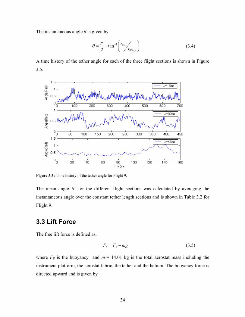
A time history of the tether angle for each of the three flight sections is shown in Figure

3.5.

Figure 3.5: Time history of the tether angle for Flight 9.

The mean angle θ for the different flight sections was calculated by averaging the

instantaneous angle over the constant tether length sections and is shown in Table 3.2 for

Flight 9.

3.3 Lift Force

The free lift force is defined as,

L BF F mg= − (3.5)

where FB is the buoyancy and m = 14.01 kg is the total aerostat mass including the

instrument platform, the aerostat fabric, the tether and the helium. The buoyancy force is

directed upward and is given by

34

B aF V gρ= (3.6)

where ρa is the density of air taken as 1.229 Kg/m3 and V = 22.45 m3 is the internal

volume of the aerostat. Using equations (3.5) and (3.6) the free lift is calculated to be

133.6 N. In order to verify the calculation, the lift was measured by tethering the balloon

to the ground indoors in a controlled environment using the Transducer Techniques load

cell. Load cell measurements were performed for about 2 minutes at 10 Hz as shown in

Figure 3.6. The graph also gives us an indication of the noise level of the sensor.

igure 3.6: Plot of the free lift measured with the Transducer Techniques load cell.

A free lift of 136.5 N, including the tether weight, was determined by averaging the data

3.4 Tension

apter 2, the tension in the cable was measured at the confluence point

F

over time; which is 3 N higher than the calculated value. This discrepancy might be

explained by the fact that the inflated balloon diameter was slightly larger than the

manufacturer’s specifications indicate. The lift measurement performed with the load cell

was considered more reliable and kept as the reference for later sections.

As mentioned in Ch

using a MLP-75 load cell from Transducer Techniques connected to a SY016 digital

amplifier board by Synectic Design. The acquisition system for the tension performed

poorly and only the tension for the November 4th flight was considered reliable. The

35

processed data for that day are shown in Figure 3.7 and compared to the free lift of

aerostat.

0 2 0 0 4 0 0 6 0 0 8 0 0 1 0 0 0 1 2 0 0 1 4 0 0 1 6 0 0 1 8 0 0 2 0 0 0- 5 0

0

5 0

1 0 0

1 5 0

2 0 0

2 5 0

3 0 0

3 5 0

4 0 0

T i m e ( s )

Tens

ion

(N)

F r e e l i f t l i n e1 3 6 . 4 9 N

Figure 3.7: Plot of the tension data for Flight 9, compared to the aerostat free lift.

The tension in the cable falls below the free lift line at certain instants in time.

This behaviour is likely caused by downward gusts, which cause a slackening of the

cable and hence decrease of the tension. To compare the tension at different tether

lengths, it was divided into 15m, 30m, 45m cable length sections as shown in Figure 3.8.

Figure 3.8: Tether tension at the different cable lengths.

36

The mean tensions at the confluence point for the different heights are shown in Table 3.3

for Flight 9.

Table 3.3: Mean tension at the different cable lengths for Flight 9

Cable length (m) Mean tension (N)

15 164.1

30 180.0

45 169.5

The mean tension in the cable at 30 m is slightly higher since the mean wind speed was 1

m/s higher then during that time period.

3.5 Wind

3.5.1 Wind Velocity, Direction and Frequency Content

The wind data was measured at 3, 5 and 10 m with wind speed recorded at 5Hz while the

wind direction was acquired every 2 and 3 seconds. Figure 3.9 shows the wind

characteristics only at 3 and 10m for clarity.

Figure 3.9: Graph of the wind speed and direction at 3 and 10 meter for Flight 9.

The convention used for the wind direction takes the angle to be zero degree when the

wind blows from true north and increases clockwise viewed from above.

37

Table 3.4 presents the wind characteristics of Flight 9 at 3m, 5m and 10m. The

wind speed turbulence intensities were calculated by taking the ratio of the wind speed

standard deviation σU to the mean wind speed U for each flight section[46].

Table 3.4: Wind characteristics of Flight 9

Height(m) wθ

(degree)

σθ

(degree) U (m/s) σU (m/s) U

Uσ

3 68.97 13.44 3.99 0.97 0.24

5 70.11 13.29 4.29 1.03 0.24

10 76.95 12.19 4.55 1.01 0.22

The frequency content of the experimental wind gives good insight about its

nature. Figure 3.10 shows the frequency spectrum of the wind of Flight 9 at 10 m height

over the entire flight. At frequencies greater than wind sensor cutoff frequency, the

amplitude drops does not drop further due to sensor noise.

Figure 3.10: Power spectrum of the wind of Flight 9 at 10 m height.

The high-frequency slope of the power spectrum can be compared to that predicted by

theory. A slope a -5/3 is consistent with the frequency distribution of a Von Karman

model[47], which will be used in Chapter 4 to generate the turbulence in the simulation.

38

3.5.2 Power Law

The wind speed and direction were measured at 3, 5 and 10 m, however the real interest

lies at heights where the aerostat is flying. Therefore it is necessary to extrapolate the

wind to higher altitudes. The following section presents how a power law model can be

used to extrapolate the wind speed at higher heights. The first step is to determine the

power law exponent that matches our experimental data. The power law model is given

by the following expression

( )m

ref ref

U z zU z

=

(3.7)

where z is the height of interest, zref the reference height which is usually taken as 10 m

[48], ( )U z is the average wind speed at the height of interest and refU is the average

wind speed at 10 m taken over the entire flight. The exponent m varies as a function of

the surface roughness, from 0.1 in the case of a very smooth water surface, to 0.4 in a

town centre. Since the wind speeds were recorded at three different heights, it was

possible to extract the exponent m for each day of flight by fitting a power law profile to

the average wind speed presented in Table 3.4. Figure 3.11 shows the results for Flight 9.

y = 3.5675x0.1077

R2 = 0.9785

3.94

4.14.24.34.44.54.64.7

0 2 4 6 8 10

Height(m)

Win

d Sp

eed(

m/s

)

12

Average wind speed

Power law fit

Figure 3.11: Plot of the average wind speed against the height for Flight 9. A power law is fitted to extract the value of the exponent.

The equation of the fitted curve was found to be ( ) 0.113.57z=U z . In order to test the

validity of the fit, equation (3.7) was rearranged into a form comparable to the power law

computed above, leading to the following expression,

39

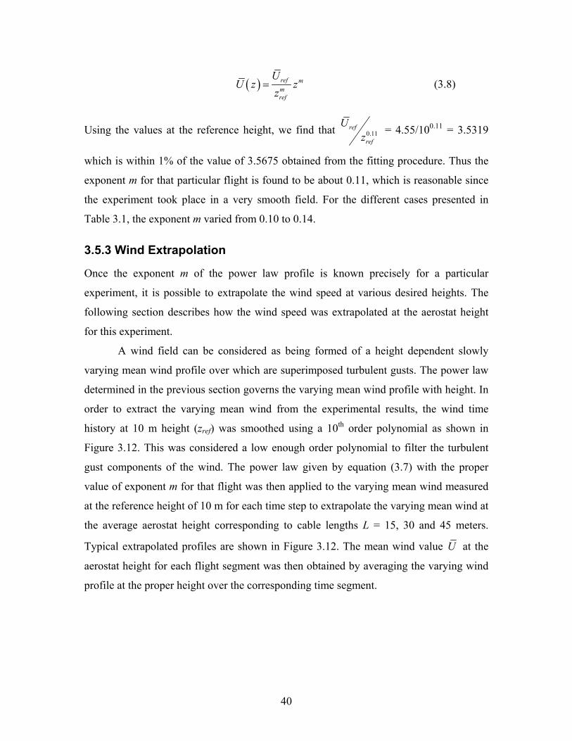
( ) ref mmref

UU z z

z= (3.8)

Using the values at the reference height, we find that 0.11ref

refzU = 4.55/100.11 = 3.5319

which is within 1% of the value of 3.5675 obtained from the fitting procedure. Thus the

exponent m for that particular flight is found to be about 0.11, which is reasonable since

the experiment took place in a very smooth field. For the different cases presented in

Table 3.1, the exponent m varied from 0.10 to 0.14.

3.5.3 Wind Extrapolation

Once the exponent m of the power law profile is known precisely for a particular

experiment, it is possible to extrapolate the wind speed at various desired heights. The

following section describes how the wind speed was extrapolated at the aerostat height

for this experiment.

A wind field can be considered as being formed of a height dependent slowly

varying mean wind profile over which are superimposed turbulent gusts. The power law

determined in the previous section governs the varying mean wind profile with height. In

order to extract the varying mean wind from the experimental results, the wind time

history at 10 m height (zref) was smoothed using a 10th order polynomial as shown in

Figure 3.12. This was considered a low enough order polynomial to filter the turbulent

gust components of the wind. The power law given by equation (3.7) with the proper

value of exponent m for that flight was then applied to the varying mean wind measured

at the reference height of 10 m for each time step to extrapolate the varying mean wind at

the average aerostat height corresponding to cable lengths L = 15, 30 and 45 meters.

Typical extrapolated profiles are shown in Figure 3.12. The mean wind value U at the

aerostat height for each flight segment was then obtained by averaging the varying wind

profile at the proper height over the corresponding time segment.

40

Figure 3.12: Plot of the fitted wind speed of Flight 9. The wind speed at 3m is shown to show how the 10th order polynomial smoothes the curve.

3.6 Drag Force and Drag Coefficient

The drag force on spheres has been a subject of research for over 50 years. Even though

extensive studies have been performed on the subject, there have been no works

investigating tethered spheres in a natural wind field. Fluid dynamists have focused their

research on fixed spheres in wind a tunnel[18]. Research on outdoor spherical helium

balloons has mainly been limited to free meteorological spheres used for wind boundary

layer measurements[24]. Some work in ocean engineering deals with effect of surface

waves on the motion of partially submerged tethered buoys, but it does not deal with drag

coefficient estimation[28]. To the authors’ knowledge only Govardhan and

Williamson[32] have systematically studied the motion of a tethered buoyant sphere and

have done so in a controlled laboratory environment. This section presents measurement

of drag forces and coefficients of a buoyant tethered spherical body in an outdoor

environment. The results are compared to those of other investigations on spherical

objects.

3.6.1 Drag Force

Since the aerostat is flying in an unsteady fluid flow, calculation of the instantaneous

drag force from the aerostat motion would require accurate knowledge of the

accelerations. Instead, the mean drag force will be calculated based upon 2 assumptions:

41

Over a long period of time, the mean acceleration is zero.

The mean z-component of the drag is negligible.

The first assumption is implicitly true for a tethered aerostat system since a non-zero

mean acceleration over a long time period would mean that the balloon is moving away

from its attachment point. For the second assumption, it is generally accepted that the

vertical mean wind in the lower planetary boundary layer is zero[49]. With these

assumptions, the analysis can be reduced to a simple static system where the tether angle

θ is the average angle between the vertical and the tether line, the drag force is the

average drag force DF and the average free lift L BF F m= − g as shown in Figure 3.13.

Figure 3.13: Ideal sketch of the aerostat equivalent static system.

From static equilibrium, the drag force DF is simply given by

( )tanD LF F θ= (3.9)

where DF is the average drag force, LF is the average free lift (136.49 N) and θ is the

average angle obtained by taking the average of the result of equation (3.4) over a flight

segment. The drag force for all flight segments was obtained using equation (3.9) and

plotted in Figure 3.14. A quadratic fit of the data is shown to highlight the quadratic

dependence of the drag force on wind velocity.

42

Figure 3.14: This figure shows the drag force versus the wind speed. A curve is fitted to demonstrate the quadratic dependence on the velocity.

3.6.2 Drag Coefficient

One of the most important physical parameters for the characterization of an aerostat is

its drag coefficient. Values of the mean drag coefficient DC can be extracted from the

known mean drag force DF by rearranging equation (2.1),

21

2

DD

a re

FCAUρ

=l

(3.10)

relU is the average velocity of the air relative to the balloon and is simply equal to the

average wind speed U since the mean aerostat velocity is zero. In order to derive

equation (3.10), it was assumed that

21 12 2D D a rel D aU A C Uρ= ≈ 2 AρF C (3.11)

where U is the instantaneous relative velocity. This approximation has been shown by

Scoggins[23] to be accurate within three percent for a free ascending sphere. Since the

velocity variations of Scoggins’ free sphere are similar to those observed in this

experiment, the approximation of equation (3.11) was considered valid. Table 3.5

presents the drag coefficients obtained for all days of experiment along with average

wind speed and other relevant information.

rel

43

Table 3.5: List of parameters of interest for the calculation of the mean drag coefficient CD

Flight Cable length L (m)

Mean wind speed U (m/s)

Reynolds Number Re (× 106)

Average angle θ (rad)

Mean Drag

DF (N)

Mean Drag Coefficient

DC Flight 1 18 2.31 0.538 0.133 18.2 0.576 Flight 2 15 3.59 0.836 0.356 50.7 0.664

15 4.17 0.971 0.467 68.9 0.668 30 4.98 1.160 0.484 71.8 0.488 Flight 3 45 4.23 0.985 0.452 66.3 0.625

Flight 4 30 2.29 0.533 0.126 17.3 0.556 15 2.38 0.554 0.175 24.1 0.718 30 3.10 0.722 0.222 30.8 0.541 Flight 5 45 3.68 0.857 0.274 38.3 0.477

Flight 6 15 3.21 0.748 0.266 37.3 0.610 15 5.85 1.362 0.576 88.7 0.437 30 7.36 1.714 0.969 198.8 0.619 Flight 7 45 7.04 1.639 0.896 170.4 0.580 15 6.08 1.416 0.708 116.8 0.533 Flight 8 30 6.30 1.467 0.744 125.6 0.533 15 4.81 1.120 0.445 65.2 0.474 30 4.97 1.157 0.468 69.1 0.471 Flight 9 45 5.28 1.230 0.519 78.99 0.471

According to published data, the drag coefficient of a smooth fixed sphere, ranges from

0.40 at Reynolds numbers less than 2 × 105 (known as subcritical), decreasing to 0.15 at

Reynolds numbers greater than 3.5 × 105 (known as supercritical). The Reynolds number

is given by

Re aUDρµ

= (3.12)

where Re is the Reynolds number, ρa = 1.229 kg/m3 is the air density, U is the average

speed of the flow, D = 3.5 m is the aerostat diameter and µ = 1.85×10-5 kg/(ms) is the

viscosity of the air at ambient condition. Our experiments were all in the supercritical

range. The mean drag coefficient of the tethered balloon was calculated to be 0.56, which

is about 4 times higher than for a fixed sphere in supercritical flow. This increase in drag

can be explained by the roughness of the aerostat and by the sphere’s oscillations to be

discussed in the next section. Williamson et al. found that the drag coefficient of a

tethered sphere in subcritical flow is about 0.75, that is about twice the drag coefficient of

44

a fixed sphere[29]. In our experiment, the drag coefficients were also found to be quite

high and constant over the range of Reynolds numbers studied and one might expect that

the supercritical drop experienced by fixed sphere in an ideal flow at the critical Reynolds

number would be much less in the case of a tethered aerostat in turbulent wind. This

behaviour is consistent with Golsdtein’s results who observed a nearly constant sphere

drag coefficient when the flow turbulence was increased[41]. Similar results were found

by increasing the surface roughness[41]. Figure 3.15 shows a plot of the drag coefficients

obtained compared to values from Wieselsberger[50] for a fixed sphere in a wind tunnel

and Scoggins[24] for free floating smooth and rough spheres. It is interesting to note that

our drag coefficients lie between those of the rough sphere and smooth sphere of

Scoggins.

Figure 3.15: Comparison of the sphere drag coefficients

45

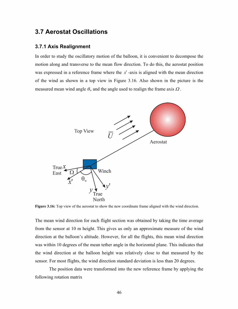
3.7 Aerostat Oscillations

3.7.1 Axis Realignment

In order to study the oscillatory motion of the balloon, it is convenient to decompose the

motion along and transverse to the mean flow direction. To do this, the aerostat position

was expressed in a reference frame where the x′ -axis is aligned with the mean direction

of the wind as shown in a top view in Figure 3.16. Also shown in the picture is the

measured mean wind angle θw and the angle used to realign the frame axis Ω .

Figure 3.16: Top view of the aerostat to show the new coordinate frame aligned with the wind direction.

The mean wind direction for each flight section was obtained by taking the time average

from the sensor at 10 m height. This gives us only an approximate measure of the wind

direction at the balloon’s altitude. However, for all the flights, this mean wind direction

was within 10 degrees of the mean tether angle in the horizontal plane. This indicates that

the wind direction at the balloon height was relatively close to that measured by the

sensor. For most flights, the wind direction standard deviation is less than 20 degrees.

The position data were transformed into the new reference frame by applying the

following rotation matrix

46

cos sinsin cosO OR

Ω ΩΩ Ω′

= −

(3.13)

where Ω is the angle between x and x′ and is related to the mean wind direction angle by

90 wθΩ = − . Table 3.6 shows the characteristics of the position data of Flight 9 after

realignment. Note that the realigned average y’ position is close to zero for all flights, this

suggests that the aerostat motion oscillates about the wind axis x′ . The average wind

direction angle θw over the 15 , 30 , and 45 m cable length sections for that day were

respectively 74.05, 80.17 and 83.16 degrees.

Table 3.6: Position data of Flight 9 after realignment

Cable Length

Average position (m) RMS of the position , ,x y zσ ′ ′ ′ (m)

xWAr ′ -6.60 2.71

WAyr ′ -0.089 4.31 15 m

WAzr ′ 16.34 1.53

xWAr ′ -13.35 5.02

WAyr ′ 0.088 6.74 30 m

WAzr ′ 29.26 2.83

xWAr ′ -21.62 7.51

WAyr ′ -0.39 9.19 45 m

WAzr ′ 40.81 2.49

3.7.2 Oscillations

As shown by Govardhan and Williamson[32], a tethered sphere in a steady fluid flow

will tend to oscillate both in the streamwise and transverse directions. The present

experiment shows that a tethered sphere also oscillates in an unsteady flow such as an

outdoor wind. Figure 3.17 presents a typical two dimensional figure ‘8’ plot of

Williamson’s sphere trajectory compared to that of our 3.5 m aerostat. It is important to

emphasize the fact that the two experiments were performed in quite different flow

conditions, as will be discussed in the next section.

47

Figure 3.17: Typical projection of the trajectory in the horizontal plane. The plot on the left shows typical figure ‘8’ motion of the Williamson’s sphere. The graph on the right presents the motion of our aerostat decomposed along and transverse to the mean flow.

It is clear from Figure 3.17, that there is less structure in our aerostat’s motion than for

Williamson’s tethered sphere. However, if closer attention is paid to the aerostat’s

trajectory by plotting the transverse and streamwise motion, it becomes apparent that the

aerostat does demonstrate oscillatory behaviour in the transverse direction as shown in

Figure 3.18 for Flight 9.

0 2 0 0 4 0 0 6 0 0 8 0 0 1 0 0 0 1 2 0 0 1 4 0 0 1 6 0 0 1 8 0 0 2 0 0 0-4 0

-2 0

0

2 0

Stre

amw

ise(

m)

0 2 0 0 4 0 0 6 0 0 8 0 0 1 0 0 0 1 2 0 0 1 4 0 0 1 6 0 0 1 8 0 0 2 0 0 0-2 0

0

2 0

4 0

Tran

sver

se(m

)

5 5 0 6 0 0 6 5 0 7 0 0 7 5 0 8 0 0 8 5 0 9 0 0 9 5 0-1 0

0

1 0

T im e (s )

Tran

sver

se(m

)

Z o o m o n t h e 1 5 m p o r t io n

Figure 3.18: Oscillatory behaviour of the aerostat for Flight 9. The top figure shows the streamwise motion of the aerostat. The two other graphs display the clear oscillatory behaviour of the aerostat in the transverse direction.

The oscillations of the balloon in the streamwise direction are not evident, most

probably due to the wind speed fluctuations. In the transverse direction, however, the

48

aerostat exhibits clear oscillations even though their amplitudes are not constant over

time. The origin of the oscillations is discussed in the next sections and an effort to

characterize and understand them is made by comparison with other research.

3.7.3 Scaling

In order for two different spheres to have similar behaviour in a fluid flow, it is important

to verify if they scale to equivalent systems. One way of doing this is to ensure that the

two spheres have the same relevant dimensionless parameters namely, the Froude number

‘Fr’, the Reynolds number ‘Re’, the Strouhal number ‘St’ and the reduced velocity Ured.

The Re number can be interpreted as the ratio of the inertia forces to the viscous forces

while the Fr number can be interpreted as the ratio of the inertia force to the gravity

force. The Re number is given by equation (3.12) and the Fr number by

2UFr

gD= (3.14)

where D is the aerostat diameter, U the average flow velocity and g the gravitational

acceleration taken to be 9.81 m/s2. The St number represents a non-dimensional

frequency of vortex shedding. It is expressed as

of DStU

= (3.15)

where f0 is the vortex shedding frequency. Finally, the reduced velocity is expressed as:

redn

UUf D

= (3.16)

where fn is the natural pendulum frequency given by

Lm

Ff

en

L

π21

= (3.17)

where FL is the free lift, me is the total mass of the aerostat including the added mass ma

(1/2 the mass of the displaced air) and L is the tether length. Table 3.7 presents a

comparison of the dimensionless parameters of the tethered sphere used by

Wiliamson[29] and of the spherical aerostat used in this experiment. This is relevant

49

since the oscillations of the Williamson sphere will be compared to those of our aerostat

in the next section. The mass ratio M*, defined as the ratio of the sphere mass to the

displaced fluid mass, is also shown in the table.

Table 3.7: Comparison of the dimensionless quantities for the aerostat used in this experiment

and the Williamson’s tethered sphere.

Re number

range

Fr number

range

St number

range

Ured Mass ratio

M*

Williamson 2×103-1.4×104 0.001-0.19 0.2 0-40 0.26-40

Our aerostat 0.51×106-

1.7×106

0.15-1.63 0.2 0-40 0.49

The two spheres cannot be considered equivalent even though they overlap for the Fr, the

Ured and the St number. The Reynolds numbers of the two systems are dinstincly

different. Consequently, some similarities might be found in their dynamics, but very

likely the two systems will behave differently. Their comparison is nevertheless of

interest since Williamson data are the only ones presently available for tethered spheres.

3.7.4 Amplitude of Oscillation

The amplitude of the transverse oscillations of the aerostat can be characterized by the

normalized amplitude, which Williamson defines as

* 2 yADσ ′= (3.18)

This quantity is plotted in Figure 3.19 as a function of the reduced velocity. Also shown

on the figure are the results of Govardhan and Williamson for the spheres of Table 3.7 for

values of Ured up to 15. They also measured values of A* at Ured above 15 (up to 40), but

these measurements were performed on spheres with values of M* greater than one and

do not compare directly to results for a buoyant sphere like ours. For this reason, the

results of Govardhan and Williamson for values of Ured above 15 are not included in

Figure 3.19.

50

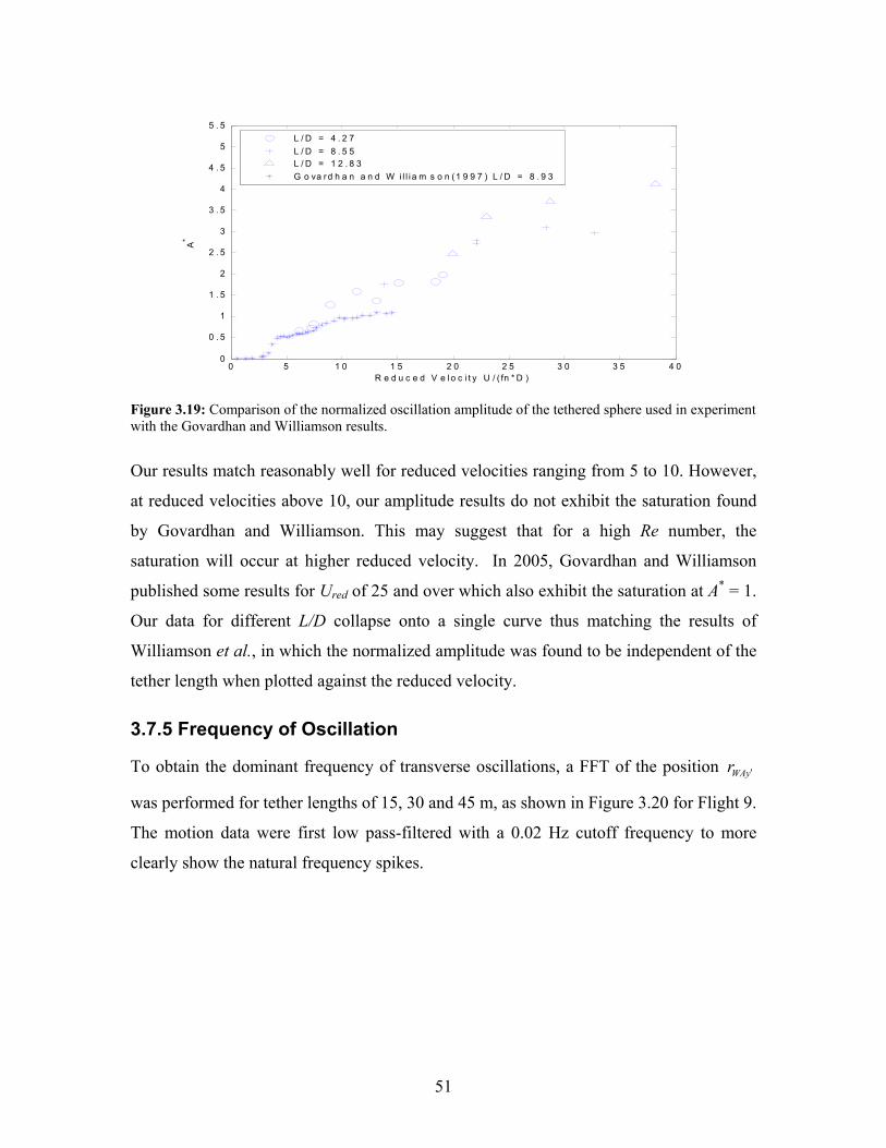
0 5 1 0 1 5 2 0 2 5 3 0 3 5 4 00

0 . 5

1

1 . 5

2

2 . 5

3

3 . 5

4

4 . 5

5

5 . 5

R e d u c e d V e lo c i t y U / ( fn * D )

A*

L / D = 4 . 2 7L / D = 8 . 5 5L / D = 1 2 . 8 3G o va rd h a n a n d W i l l i a m s o n (1 9 9 7 ) L / D = 8 . 9 3

Figure 3.19: Comparison of the normalized oscillation amplitude of the tethered sphere used in experiment with the Govardhan and Williamson results.

Our results match reasonably well for reduced velocities ranging from 5 to 10. However,

at reduced velocities above 10, our amplitude results do not exhibit the saturation found

by Govardhan and Williamson. This may suggest that for a high Re number, the

saturation will occur at higher reduced velocity. In 2005, Govardhan and Williamson

published some results for Ured of 25 and over which also exhibit the saturation at A* = 1.

Our data for different L/D collapse onto a single curve thus matching the results of

Williamson et al., in which the normalized amplitude was found to be independent of the

tether length when plotted against the reduced velocity.

3.7.5 Frequency of Oscillation

To obtain the dominant frequency of transverse oscillations, a FFT of the position WAyr ′

was performed for tether lengths of 15, 30 and 45 m, as shown in Figure 3.20 for Flight 9.

The motion data were first low pass-filtered with a 0.02 Hz cutoff frequency to more

clearly show the natural frequency spikes.

51

0 0.05 0.1 0.15 0.2 0.25 0.3 0.35 0.4 0.45 0.50

1

2x 106 Power Spectrum of the Tranverse motion at 15m

0 0.05 0.1 0.15 0.2 0.25 0.3 0.35 0.4 0.45 0.50

2

4x 106 Power Spectrum of the transverse motion at 30m

0 0.05 0.1 0.15 0.2 0.25 0.3 0.35 0.4 0.45 0.50

1

2x 107 Power Spectrum of the Transverse motion at 45m

Frequency (Hz)

Natural frequency

Figure 3.20: Power spectrum of the transverse motion for Flight 9

The power spectra for the different days of experimentation all exhibit a sharp peak

within 30% of the system’s natural pendulum frequency given by equation (3.17). As

expected, the dominant frequency of the power spectrum decreases as the tether length

increases. Table 3.8 presents a list of the dominant frequency components at tether

lengths of 15, 30 and 45m compared with the theoretical pendulum frequency of the

system. The dominant frequency component corresponds to the largest peak in the

frequency spectrum.

Table 3.8: Comparison of the dominant frequency in power spectrum with the theoretical pendulum

frequency of the system for Flight 9

Cable length (m) Dominant frequency

component (Hz)

Theoretical pendulum

frequency (Hz)

15 0.09 0.0910

30 0.07 0.0643

45 0.06 0.0525

52

3.7.6 Nature of the Oscillations

A considerable amount of work on flow-induced vibrations is reported in the literature. In

most cases, the systems studied consist of elastically mounted cylinders[51]. A small

amount of research has also been dedicated to tethered cylinder oscillations[52] and even

less to tethered spheres. Among the works on tethered spheres, those of Williamson are

the most systematic but there remains a great deal of research to be done on the subject.

For example, up to now no research has been performed on a tethered sphere in the

supercritical flow regime. With the available data, it is difficult to provide a definite

explanation as to what causes our aerostat to oscillate strongly, although in the light of

previous research, various possible scenarios can be conjectured from which one seems

the most likely.

The fact that the system oscillates transversely gives insight into the

characteristics of the force acting on the aerostat. It first suggests that the force must act

transverse to the flow. Also it must have a strong component close to the natural

frequency to excite the system at this same frequency. Williamson and al. [29] [30] [53]

have hypothesised that the oscillation of a tethered sphere in a fluid flow results from the

periodic vortex shedding in the wake of the sphere at a frequency close to the tethered

aerostat’s natural frequency. These vortices create a periodic force called shedding force

that drives the sphere close to its natural frequency; this is called the “lock in”

phenomenon. The vortex shedding characteristics are highly dependent on the Reynolds

number and are usually determined based on results measured for fixed sphere[42].

However, Tenada [20] and Sakamoto and Haniu [18] have shown that periodic vortex

shedding does not occur for a fixed sphere for flow above Reynolds number of 2×104.

Since all our experiment were performed at greater Reynolds numbers, the oscillations

seen in Figure 3.18 cannot be explained as a classical “lock in” of the principal vortex

shedding frequency with the system’s natural pendulum frequency.

The ‘lock in’ scenario having been rejected, four other possible scenarios were

investigated:

Scenario 1: Turbulence input provided by the wind, with very low system

damping. The system responds at the natural frequency.

53

This scenario envisions that there is no vortex shedding at all from the sphere, and that

the variations in drag forces on the sphere are solely due to the variations in magnitude

and direction of the upstream wind due to its turbulence content of the wind. If the lateral

system dynamics is only very lightly damped, then perhaps even a small amount of

turbulence content at the natural frequency might elicit a strong response at that

frequency. However, our existing aerostat model shows a damping ratio of 0.18 at 1 m/s,

with the damping ratio increasing linearly with speed (this will be further discussed in the

next chapter). Thus, this scenario would only be possible at very low speeds. This

interpretation is unlikely since the forcing input to the system due only to upstream

turbulence tends to be quite weak.

Scenario 2: Broadband vortex shedding in the wake of the sphere, the system

responds at its natural frequency.

This scenario takes into account that, at high Reynolds numbers past the supercritical

drop, vortex shedding is known to occur at a broad range frequencies as mentioned by

Willmarth and Enlow[21]. Thus, this scenario would provide a stronger forcing input to

the system and might elicit stronger reactions than scenario 1. However, it still relies on

relatively light lateral damping, unless the frequency content at the natural frequency is

particularly strong.

Scenario 3: Fluid-structure interaction causing a periodic force at the critical

Reynolds number.

This scenario considers the generation of pressure differential on the two (lateral)

sides of the sphere created by the side-to-side acceleration of the sphere, as speculated by

Kruchinin[25]. He hypothesised that this pressure change due to motion would delay

transition on one side of the sphere and accelerate it on the other side, thus causing an

unsteady transition near the critical regime. He also showed that, if this side force has a

time delay with respect to the acceleration, it could result in strong oscillations. For our

experiment, this scenario is unlikely since Kruchinin demonstrated experimentally that

the phenomenon occurs only close to the critical Reynolds number. For our aerostat, due

to the presence of upstream turbulence on the order of 20-30%, we can expect that our

critical Re is likely below 1×105. Our operational Reynolds numbers were closer to 3×105

54

and up. Thus, our expectation is that the flow is clearly supercritical for all flights and

that, by itself, seems to preclude this scenario.

Scenario 4: Oscillation generated from ‘movement-induced excitation’.

Jauvtis et al., discovered in 2001[53], an unexpected mode of oscillation of the tethered

sphere at high-reduced velocity outside the ‘lock in’ regime. In other words, they found

highly periodic motion close to the natural frequency of the sphere at a speed for which

the static body would exhibit between three or eight vortex structures. This regime starts

at reduced velocity close to 15 and remains up to 40. This falls almost exactly in the

range of operation of our aerostat. Govardhan and Williamson demonstrated in 2005 that

these oscillations are due to ‘movement induced excitation’[32]. In absence of motion,

these forces would be absent. However, if the system is perturbed and vibrates in the

transverse direction, it creates a self-sustaining vortex force to pump energy into the

system and increase the amplitudes of oscillation close to the natural frequency. They

also found that this phenomenon was independent of the Reynolds number over which

they performed the experiments that is, Re = 3000-9000. If we assume that this

phenomenon is fully independent of the Reynolds number, it would provide an

explanation for the transverse oscillations that our aerostat exhibits.

55

Chapter 4

Simulation of a Tethered Spherical Aerostat

This chapter focuses on the dynamics modelling of a spherical tethered aerostat, as used

in the experiment. In order to account for the effect of the instrument platform on the

balloon, some additions were made to an existing model developed by Lambert[4]. The

physical properties of the aerostat are determined and the simulation is validated by

comparing its results with experimental data. Finally the equations of motion of the

system are linearized and a modal analysis of the system is performed.

4.1 Original Model

The simulation developed in this work was based on an existing numerical model created

by Lambert[4]. The original model was developed during a preliminary analysis of the

LAR concept, and has been used to study the controllability of the radio telescope

receiver[54] and the stability of the system[14]. Originally, the simulation included a

model of a spherical and a streamlined aerostat attached to the ground by a single cable

and subjected to a turbulent wind field. In the following description, only the spherical

aerostat will be discussed. The original dynamics model was obtained by discretizing the

tether into a series of elements and then solving for the motion by integrating the

dynamic equations in an inertial frame. A 2-D schematic of the original model is

presented in Figure 4.1

56

Figure 4.1: 2-D sketch of the original model showing the discretization of cable.

4.1.1 Cable Model

The original simulation uses a lumped-mass model of the cable. In this type of model, the

cable is first discretized into a series of n elements and the mass of each element is

lumped into its end nodes. Two types of forces were taken into account in modelling the

tether, the external forces and the internal forces. The external forces originate from the

tether interactions with the environment and include the aerodynamic drag and gravity.

The internal forces include the internal damping modeled as a viscous dashpot of

damping coefficient CV and the axial stiffness modeled as a spring of stiffness K as

illustrated in Figure 4.2. The cable is considered to have negligible bending stiffness. The

lumped mass approximation allows for the motion of each node to be calculated

independently in the three degrees of freedom resulting in a set of 3n equations of motion

(not including the fixed node 0). The lumped mass model has been validated for a

variety of underwater systems with excellent agreement[55] with insitu measurements.

57

Figure 4.2: Cable element and node representation

4.1.2 Aerostat Model

The aerostat is modeled as a point mass located at the upper node of the tether. It is

subject to buoyancy, gravity and aerodynamic drag generated by the wind. Modelling the

aerostat as a point mass was justified by assuming that the centre of gravity (CG) of the

system was coincident with the centre of buoyancy (CB) and the aerodynamic centre

(CP). As a result, there would be no moment acting on the aerostat and it would act as an

ideal point mass. The mass of the aerostat included the ‘added mass’ of the buoyant

sphere[56] which is one half of the air mass it displaces.

4.1.3 Wind Model

A wind model is incorporated to determine the effects of the turbulent wind acting on the

tethered aerostat system. The wind model consists of a height-dependent mean wind (low

frequency wind) on which is superimposed a wind gust model (high frequency wind).

The relationship between the mean wind and the height is governed by a power law as

discussed in Section 3.5.2. The turbulent gusts were generated based on desired

statistical properties including the turbulence intensity, scale length and spectra [54]. The

turbulence model was adjusted for accuracy at heights above 100 m, and thus needed

improvement in the lower planetary boundary layer (<100m) where our experiment was

performed. Those improvements are presented in Section 4.2.2.

58

4.2 Proposed Model

The original model was not capable of accounting for the lowering of the aerostat CG due

to the presence of the instrument platform, and the new model takes this effect into

account. The presence of an off-centre load (the platform) on the aerostat will shift the

aerostat CG and thus introduce rotational moments because the centers of gravity and

pressure are no longer coincident. The balloon no longer behaves as a point mass but

must be modelled as a rigid body by introducing the three rotational equations of motions

(EOM). In the following section, the modified EOM are presented, along with the new

motion variables. In addition to the aforementioned changes, a new wind model that

better predicts the wind behaviour in the lower planetary boundary layer is introduced.

In the previous model, the centre of gravity and the last node were located at the

end of the last tether element as shown in Figure 4.1. For the proposed model, the

aerostat and the secondary lines are treated as a single rigid body with the last node

located at the confluence point, and the last element defined from the n-1th node to the

confluence point as shown in Figure 4.3.

Figure 4.3: Idealized sketch of the proposed aerostat model. rT is the vector from center of gravity to the confluence point and FT is the resultant force of the last element acting on the aerostat.

59

4.2.1 Equations of motion

The dynamic simulation is obtained by setting up and solving simultaneously all the

equations of motion in 3-D space. These include the 3n EOM of the tether nodes as

discussed in the previous section plus the six translational and rotational EOM of the

aerostat. The coupling of the tether model and the aerostat model was achieved by

connecting the upper end of the last element of the tether to the confluence point of the

aerostat as shown in Figure 4.3. Also shown on the figure is the force from the nth

element FT. This force is included in the equations of motion of the aerostat.

Aerostat

The motion of the aerostat is defined as the relative position and orientation of a

body-fixed coordinate frame attached to the aerostat CG with respect to an inertial frame

located at an arbitrary point on the ground as shown in Figure 4.4.

Figure 4.4: Idealized sketch of the aerostat system showing the body-fixed and inertial frames.

The translational motion is given by Newton’s second law and can be written as:

aF em= (4.1)

where F is the net force applied to the aerostat, me is its mass including the added mass

and the acceleration of the centre of mass with respect to the inertial frame. The

acceleration of the aerostat is obtained by taking the derivative of the velocity with

a

60

respect to the inertial frame, ddt

cmV . This is related to the rate of change of the velocity

in the body framet

δδ

cmV by the following expression:

e

dm dt t

δδ

= = + ×cm cm cmcm

F V V ω V (4.2)

where V = [u v w]cmT is the velocity of the aerostat in the body frame and [ ]Tp q r=ω

is the angular velocity of the system. The rotational motion of the aerostat is governed by

Euler’s equation:

xx xy xz

xy yy yz

xz yz zz

I I II I II I I

− − = + × = − − − −

&cm cm cmM I ω ω Iω I (4.3)

where is the inertia tensor about the centre of mass and is the net moment acting

on the aerostat with respect to the CG. For our system,

cmI cmM

xy 0xz yzI I I= = = due to two

planes of symmetry.

The forces and moment acting on the aerostat come from four sources: the

buoyancy, the gravity, the aerodynamics and the tether tension. These are shown in

Figure 4.5.

Figure 4.5: Free body diagram of a tethered sphere in a fluid flow

61

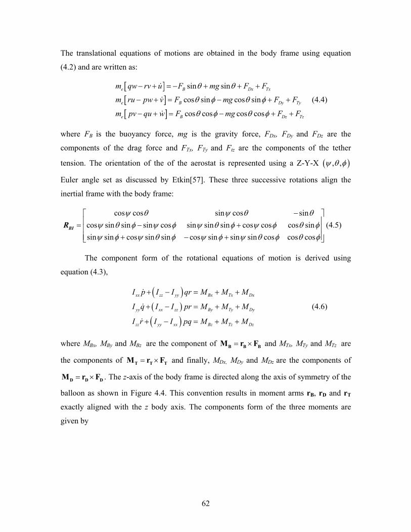
The translational equations of motions are obtained in the body frame using equation

(4.2) and are written as:

[ ][ ][ ]

sin sin

cos sin cos sin

cos cos cos cos

e B Dx Tx

e B

e B

m qw rv u F mg F F

m ru pw v F mg F F

m pv qu w F mg F F

θ θ

θ φ θ φ

θ φ θ φ

− + = − + + +

− + = − + +

− + = − + +

&

&

&

Dy Ty

Dz Tz

(4.4)

where FB is the buoyancy force, mg is the gravity force, FDx, FDy and FDz are the

components of the drag force and FTx, FTy and Ftz are the components of the tether

tension. The orientation of the of the aerostat is represented using a Z-Y-X ( ), ,ψ θ φ

Euler angle set as discussed by Etkin[57]. These three successive rotations align the

inertial frame with the body frame:

cos cos sin cos sin

cos sin sin sin cos sin sin sin cos cos cos sinsin sin cos sin sin cos sin sin sin cos cos cos

ψ θ ψ θ θψ θ φ ψ φ ψ θ φ ψ φ θ φψ φ ψ θ φ ψ φ ψ θ φ θ

− = − + + − +

BI

φR (4.5)

The component form of the rotational equations of motion is derived using

equation (4.3),

( )( )( )

xx zz yy Bx Tx Dx

yy xx zz By Ty Dy

zz yy xx Bz Tz Dz

I p I I qr M M M

I q I I pr M M M

I r I I pq M M M

+ − = + +

+ − = + +

+ − = + +

&

&

&

(4.6)

where MBx, MBy and MBz are the component of = ×B BM r FB

T

D

and MTx, MTy and MTz are

the components of and finally, M= ×T TM r F Dx, MDy and MDz are the components of

. The z-axis of the body frame is directed along the axis of symmetry of the

balloon as shown in Figure 4.4. This convention results in moment arms r

= ×D DM r F

B, rD and rT

exactly aligned with the z body axis. The components form of the three moments are

given by

62

cos sinsin

0

0

0

Bx Bz B

By Bz B

Bz

Dx Dz Dy

Dy Dz Dx

DZ

Tx Tz Ty

Ty Tz Ty

Tz

M r FM r F

MM r F

M r F

MM r F

M r F

M

θ φθ

= −

= −

== −

=

== −

=

=

(4.7)

where rBz is the z component of the buoyancy moment arm going from CG to CB, rDz is

the z component of the drag moment arm going form CG to CP and rTz is the z component

of the tension moment arm going from CG to the confluence point. According to the axis

convention of the body frame, rBz and rDz are positive while rTz is negative.

Tether

The equation of motion for the ith node of the tether is

i im i=F a (4.8)

where Fi is the sum of the external acting on the tether node and ai is the node

acceleration. More specifically, equation (4.8) can be written as

( ) ( )( ) ( ) ( ) ( )( )1 1 1 112i i Ti Pi Di iT i P i D i im m+ + + += + − + + + + +a F F F F F F mg g (4.9)

where is the tension force, TF PF is the internal damping force, DF is the aerodynamic

drag force vector and mig is the gravitational force. The expression for these forces are

well described by Nahon et al. [54] The subscript i and i+1 specify the elements

involved. Note that the mass mi corresponds to the mass of one cable element.

Complete system

The complete system is composed using equations (4.4), (4.6) for the aerostat and

equation (4.9) for the tether. Assuming that the number of element is n, the total number

of nodes will be n+1 as shown in Figure 4.3. This second order system is reduced to a

first order system with the state vector in the inertial frame organized as follow:

63

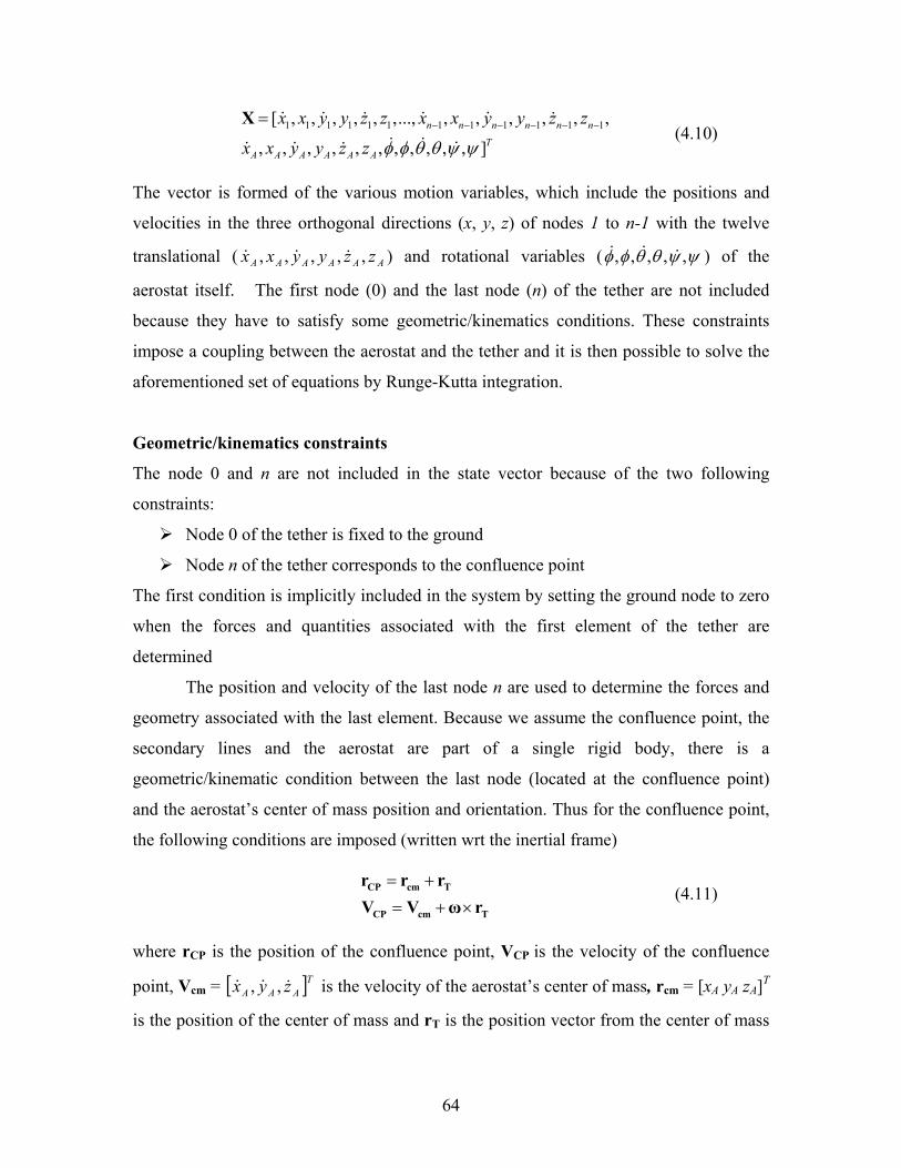
1 1 1 1 1 1 1 1 1 1 1 1[ , , , , , ,..., , , , , , ,

, , , , , , , , , , , ]n n n n n n

TA A A A A A

x x y y z z x x y y z z

x x y y z z φ φ θ θ ψ ψ− − − − − −=X & & & && &

& & && & & (4.10)

The vector is formed of the various motion variables, which include the positions and

velocities in the three orthogonal directions (x, y, z) of nodes 1 to n-1 with the twelve

translational ( ) and rotational variables ( ) of the

aerostat itself. The first node (0) and the last node (n) of the tether are not included

because they have to satisfy some geometric/kinematics conditions. These constraints

impose a coupling between the aerostat and the tether and it is then possible to solve the

aforementioned set of equations by Runge-Kutta integration.

AAAAAA zzyyxx ,,,,, &&& ψψθθφφ ,,,,, &&&

Geometric/kinematics constraints

The node 0 and n are not included in the state vector because of the two following

constraints:

Node 0 of the tether is fixed to the ground

Node n of the tether corresponds to the confluence point

The first condition is implicitly included in the system by setting the ground node to zero

when the forces and quantities associated with the first element of the tether are

determined

The position and velocity of the last node n are used to determine the forces and

geometry associated with the last element. Because we assume the confluence point, the

secondary lines and the aerostat are part of a single rigid body, there is a

geometric/kinematic condition between the last node (located at the confluence point)

and the aerostat’s center of mass position and orientation. Thus for the confluence point,

the following conditions are imposed (written wrt the inertial frame)

= += + ×

CP cm T

CP cm T

r r rV V ω r

(4.11)

where rCP is the position of the confluence point, VCP is the velocity of the confluence

point, Vcm = is the velocity of the aerostat’s center of mass, r[ TAAA zyx &&& ,, ] cm = [xA yA zA]T

is the position of the center of mass and rT is the position vector from the center of mass

64

to the confluence point. These condition are imposed at each time step during the Runge-

Kutta integration.

4.2.2 Revised Wind Model

A new wind model was developed to correct the inaccuracies of the original model at

altitudes below 50m. As for the original model, it consists of a height dependent mean

wind profile over which are superimposed turbulent gusts. The mean wind U at height z

is represented by a power law profile [48] as discussed in Section 3.5.2 to represent the

planetary boundary layer,

m

gg

zU Uz

=

(4.12)

where the exponent m was determined based on experimental results for each flight. A

gradient height zg = 300 m was used at which the mean wind speed saturates to a value

gU . The gradient velocity gU was calculated based on our experimental conditions

measured at z = 10 m using equation (4.12):

1030010

m

gU U =

(4.13)

where 10U is the mean wind speed at 10 m and the exponent was determined using the

procedure discussed in Section 3.5.2.

The original wind gust model was not intended for the terrain and the heights in

which this experiment was performed and a new turbulence model had to be developed.

The relationship between the turbulence intensities in the x, y and z directions with height

was based on ESDU curves[58] shown in Figure 4.6. Also shown in the figure, are the

experimental intensities in the x direction at an altitude of 10 m.

65

Figure 4.6: Comparison of the turbulent intensities vs. height from various sources. A zoom on heights below 50 m is presented to better show the region of interest.

The ESDU turbulence intensities σu, σv, σw, in the three orthogonal directions were

introduced in simulation by fitting a curve through the ESDU data, leading to the

following relations:

( )

( )0 .0 1

0 .05 50050 0

0 .05 0 .032 300 500200

13 .51 3 .23 300

u

z mz

m z mU

z mz

σ

≥ −= + ≤ < − <

( )

( )0.01

0.05 500500

0.05 0.012 300 500200

12.13 1.95 300

v

z mz

m z mU

z mz

σ

≥ −= + ≤ < − <

( )0.01

0.05 300

11.17 1.06 300

w

z m

Uz mz

σ

≥

=

− <

(4.14)

66

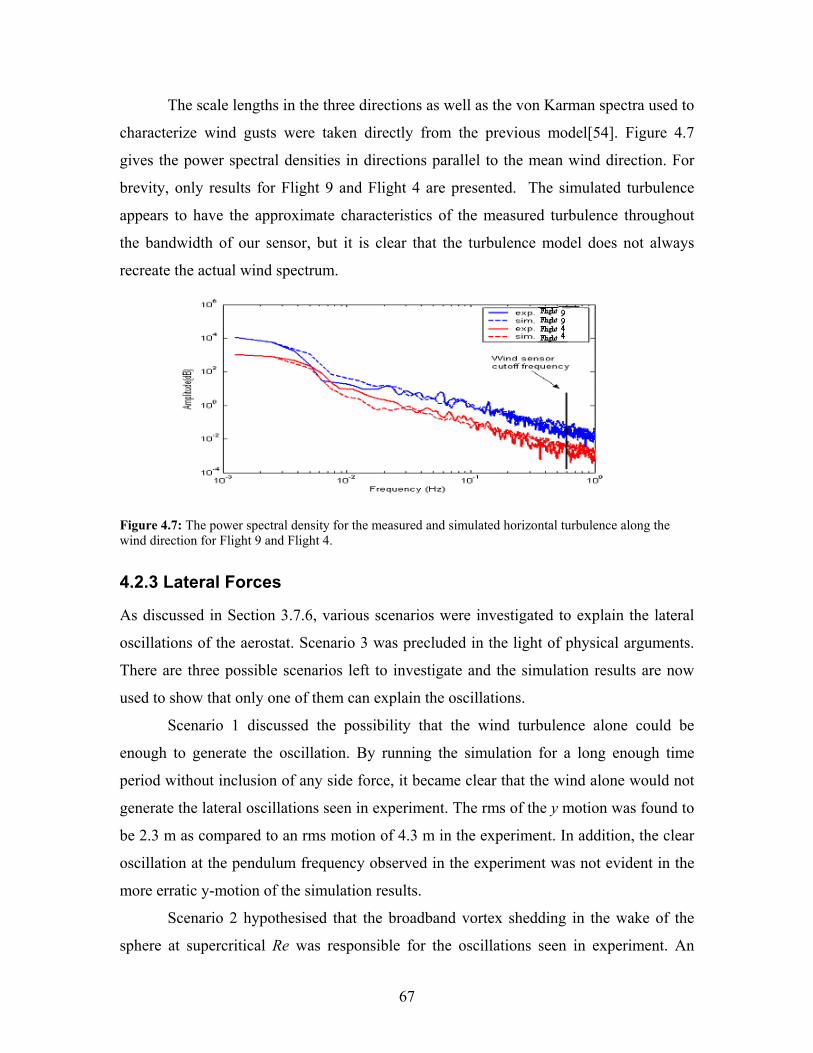
The scale lengths in the three directions as well as the von Karman spectra used to

characterize wind gusts were taken directly from the previous model[54]. Figure 4.7

gives the power spectral densities in directions parallel to the mean wind direction. For

brevity, only results for Flight 9 and Flight 4 are presented. The simulated turbulence

appears to have the approximate characteristics of the measured turbulence throughout

the bandwidth of our sensor, but it is clear that the turbulence model does not always

recreate the actual wind spectrum.

Figure 4.7: The power spectral density for the measured and simulated horizontal turbulence along the wind direction for Flight 9 and Flight 4.

4.2.3 Lateral Forces

As discussed in Section 3.7.6, various scenarios were investigated to explain the lateral

oscillations of the aerostat. Scenario 3 was precluded in the light of physical arguments.

There are three possible scenarios left to investigate and the simulation results are now

used to show that only one of them can explain the oscillations.

Scenario 1 discussed the possibility that the wind turbulence alone could be

enough to generate the oscillation. By running the simulation for a long enough time

period without inclusion of any side force, it became clear that the wind alone would not

generate the lateral oscillations seen in experiment. The rms of the y motion was found to

be 2.3 m as compared to an rms motion of 4.3 m in the experiment. In addition, the clear

oscillation at the pendulum frequency observed in the experiment was not evident in the

more erratic y-motion of the simulation results.

Scenario 2 hypothesised that the broadband vortex shedding in the wake of the

sphere at supercritical Re was responsible for the oscillations seen in experiment. An

67

attempt to introduce the resulting broadband force based on the spectral density provided

by Willmarth and Enlow [21] at a Re close to that of our aerostat demonstrated that there

would not be enough content at the natural frequency to induce the lateral oscillations

seen in experiment. The rms of the y motion was found to be 2.51 m, which is still much

less than the experiment rms of 4.3 m and the oscillations observed in the experiment

were again absent in the simulation.

Thus the possibility of self-induced forced oscillations seemed to be the last

remaining scenario possibility. Govardhan and Williamson discussed a method to

characterize the forces responsible for the transverse oscillation by treating the aerostat as

simple second order system[32]. This method is used extensively in the literature to

describe vortex induced vibration[34]. One can formulate the equation of motion as:

em y cy ky Fvortex+ + =&& & (4.15)

where 2 nc emω ζ= is the structural damping with ζ being the damping coefficient,

Fvortex is transverse vortex force and k is the spring constant. For self-induced oscillation

the vortex force Fvortex(t) is represented well by a sinusoidal force at the frequency of oscillation

ω as discussed by Govardhan and Williamson in 2005[32]. For the aerostat, the oscillations

occur at the natural frequency, which implies that ω = ωn = e

km

The response amplitude Yamp may be derived in a straightforward manner from

equation (4.15):

022amp

e n

FYm ζω

= (4.16)

where F0 is the amplitude of Fvortex. Equation (4.16) can be used to deduce F0, the

magnitude of the transverse vortex force necessary to create the motion amplitude Yamp, as

follows

( ) ( )20 sin 2 sinvortex n amp e n nF F t Y m tω ζω ω= = (4.17)

The damping ratio was determined based on value given by the linear analysis as

discussed in Section 4.5.5. The saturation amplitude Fmax of the vortex force was set

68

based on Govardhan and Williamson’s results for a tethered sphere in the same reduced

velocity range[32]:

( )2max max

12 aF C AUρ= (4.18)

where Cmax is the amplitude of the normalized vortex force measured by Govardhan and

Williamson Cvortex. According to them Cmax = 0.2 for the case of a tethered sphere in the

reduced velocity range of our aerostat. This led, for example, to a force of 27.7 N for the

mean wind U = 5.27 m/s experienced during Flight 9 at L = 45m.

To simulate the effect of self-induced excitation, the following procedure was adopted

1) The simulation is started including wind turbulence

2) The rms value of y is computed at each time step. The rms value is used to

calculate the lateral motion amplitude 2amp rms=Y y .

3) As the motion amplitude increases, the magnitude of the sinusoidal lateral

force increases according to equation (4.17).

4) When the maximum force amplitude Fmax is reached, the magnitude of the

sinusoidal lateral force is set constant to Fmax.

4.3 Physical Parameters

In order to solve the equations of motion outlined earlier we must specify the physical

parameters consistent with the aerostat system used in the experiment. These are

presented in the following section, along with the methodology to determine them. They

include those parameters pertaining to the tether and those pertaining to the aerostat itself.

4.3.1 Aerostat parameters

Most physical parameters such as the aerostat net lift and diameters were extracted from

direct measurement. To obtain the remaining parameters, a three-dimensional CAD

model was generated using PRO-E. The CAD model was constructed to accurately

represent the actual aerostat, complete with the thin-walled shell of the hull, the contained

helium, which is considered to be rigid, and the instrument platform with the sensors

positioned appropriately. The experimental platform CAD drawing is shown on Figure

69

2.14. The appropriate density was assigned to each part, and the various parameters were

obtained using PRO-E. The mass, volume and inertia moments are presented in Table 4.1

as well as various geometrical parameters.

Table 4.1: Physical parameters

Parameter Value Parameter Value

Aerostat

diameter 3.5 m

Centre of buoyancy

and of pressure

(from CG):

Aerostat volume 22.45 m3 rBx, rDx 0.0 m

Helium mass 3.79 kg rBy, rDy 0.0 m

Platform mass 3.69 kg rBz, rDz 0.52 m

Hull mass (no

helium) 6.52 kg

Confluence point

(form CG)

Total mass m 14.0 kg rTx 0 m

Helium density 0.169 kg/ m3 rTy 0.0 m

Air density 1.229 kg/ m3 rTz -3.66 m

Buoyancy FB 270.39 N Drag Coefficient

(CD) 0.56

Total lift 132.69 N

Centre of gravity

(from bottom

centre):

Inertia tensor

components:

xcm 0.0 m Ixx 25.64 kg⋅m2

ycm 0.0 m Iyy 25.64 kg⋅m2

zcm 1.23 m Izz 16.44 kg⋅m2

4.3.2 Tether Parameters

Most of the Plasma tether parameters were provided by the manufacturer Cortland Cable.

The damping ratio and the elastic modulus were estimated from experimental tests

performed by Lambert [4] and the area of the cross section was determined in laboratory

70

test. The normal drag coefficient was estimated by assuming the cable has a cylindrical

profile. Table 4.2 presents a list of the relevant tether parameters.

Table 4.2: Tether parameters

Parameters Value

Cross section area At 1.76×10-6 m2

Density ρt 840 kg/m3

Elastic modulus E 38 Gpa

Damping ratio ζt 0.017

CDt 1.2

4.4 Non-linear Simulation Results and Comparison

The ultimate validation of a model comes from its ability to represent reality. Flight 9

was selected as the basis for comparison because the three tether length flight sections are

sufficiently representative of the results for the different days of experimentation. For the

comparison, the x-axis is aligned along the direction of the mean wind, the y-axis is

transverse to wind and the z-axis is directed along the gravity vector.

Since the wind speed is responsible for the majority of the dynamics of the

system, the following steps were taken to ensure that the wind field in the simulation was

statistically similar to the infield measurements:

1. the mean wind at 10m refU was determined as discussed in Section 3.5.3

2. the vertical profile of the basic wind field was generated using a power-law

boundary layer profile as discussed in Section 3.5.3

3. the turbulence was adjusted in simulation to match the measured turbulence

for the test period.

Table 4.3 presents a comparison of measured and simulated data for aerostat

position and tether tension. A comparison of the normalized amplitude A* of the lateral

motion is also presented. Figures 4.8 and 4.9 present a comparison of the time history of

measured and simulated results for Flight 9 at a cable length of 15 m for a representative

subset of 200 s. The time history of the simulated and experimental results is not

expected to be identical since the simulated wind turbulence was generated based on

71

statistical properties. In order to directly compare the time history of the dynamics

variables, a precise measurement of the wind at the aerostat altitude would have to be

imported in the code.

Table 4.3: Comparison of experimental and simulated results for the three flight sections of Flight 9

Flight 9 L=15m

Flight 9 L=30m

Flight 9 L=45m Measured

paramater Exp. Sim. % Exp. Sim. % diff. Exp. Sim. %

diff. xWAr ′ -6.6 -7.91 20.0 -13.35 -14.48 8.46 -21.6 -23.82 9.2

yWAr ′ 0.09 0.33 - 0.09 0.69 - -0.39 1.21 -

zWAr ′ 16.34 16.39 0.3 29.26 29.17 0.3 40.81 41.81 2.4

σx 2.71 2.61 -3.8 5.02 4.41 -12.2 7.51 4.46 -40.2σy 4.31 3.07 -28.8 6.72 4.63 -31.1 9.19 5.91 -35.7

Aerostat position

(m)

σz 1.53 1.23 -19.6 2.83 2.29 -19.1 6.22 2.49 -60.1A* in y

direction A* 1.8 1.24 -31.1 2.72 1.89 -30.5 3.71 2.44 -34.2

Tether angle

(degree) θ 25.2 23.5 -6.8 26.9 25.21 -6.3 29.2 26.9 -7.8

T 164.1 153.4 -6.5 180.0 153.0 -15.0 169.5 154.3 -8.9 Tension (N)

σT 40.1 23.3 -41.8 48.0 22.5 -53.2 38.5 19.5 -49.2

Even though the simulation and experiment tend to exhibit similar behavior, the

error between the various results can be as high as 60%. The discrepancies in the results

for the different tether lengths present some clear trends and it is possible to identify the

source for most of them. The results for the mean x-position are quite good. However, the

error on the standard deviation seems to increase with tether length with the experimental

standard deviation being higher. This can be attributed to the fact the experimental wind

direction was varying. The experimental x-results were aligned with the mean wind

direction and not the instantaneous one, thus some of the transverse oscillations appear in

the experimental x-position as can be seen in the top graph of Figure 4.8. This results in

an increase of the experimental x-standard deviation.

The mean simulated and experimental y-position, are off by up to 1 m and the

oscillation amplitudes are smaller in the simulation than in the experiment. The fact that

the oscillation are smaller in simulation suggests that the sinusoidal lateral force

72

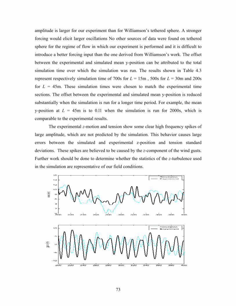
amplitude is larger for our experiment than for Williamson’s tethered sphere. A stronger

forcing would elicit larger oscillations No other sources of data were found on tethered

sphere for the regime of flow in which our experiment is performed and it is difficult to

introduce a better forcing input than the one derived from Williamson’s work. The offset

between the experimental and simulated mean y-position can be attributed to the total

simulation time over which the simulation was run. The results shown in Table 4.3

represent respectively simulation time of 700s for L = 15m , 500s for L = 30m and 200s

for L = 45m. These simulation times were chosen to match the experimental time

sections. The offset between the experimental and simulated mean y-position is reduced

substantially when the simulation is run for a longer time period. For example, the mean

y-position at L = 45m is to 0.l1 when the simulation is run for 2000s, which is

comparable to the experimental results.

The experimental z-motion and tension show some clear high frequency spikes of

large amplitude, which are not predicted by the simulation. This behavior causes large

errors between the simulated and experimental z-position and tension standard

deviations. These spikes are believed to be caused by the z-component of the wind gusts.

Further work should be done to determine whether the statistics of the z-turbulence used

in the simulation are representative of our field conditions.

73

Figure 4.8: Comparison of experimental and simulated results for the aerostat position for Flight 9 at L=15m

Figure 4.9: Comparison of the experimental and simulated results for the tether tension for Flight 9 at L=15m

4.5 Linear Model

A non-linear model is interesting in the sense that it provides some understanding of the

dynamics of our system in the time domain. However, it provides a very limited

understanding of the system since no clear conclusions can be drawn concerning the

modes of oscillation of the system. In order to analyse the model in the frequency domain

and answer questions such as: What are the predicted modes of oscillation? What are the

frequencies and damping of these modes? Are the modes of oscillation close to those

predicted by theory?, a linear model is required. The following section discusses the

linearization of the E.O.M. discussed in Section 4.2.1. An examination of the

eigenvectors and eigenvalues then allows us to determine the behaviour of the aerostat in

the frequency domain.

74

4.5.1 Description and Validation of the Linear Model

The dynamics simulation of a system can be thought as a set of functional relationships

where the derivative of each state variable is dependent on the full set of state variables.

This is well represented by the following relationship:

(4.19) ( )=X f X&

where 1 1 1 1 1 1[ , , , , , ,..., , , , , , , , , , , , ]Tn n n n n nx x y y z z x x y y z z φ φ θ θ ψ ψ=X & & && & & && & is the state vector. The

vector is formed of the various motion variables, which include the positions and

velocities in the three orthogonal directions (x, y, z) of each of the n last nodes with the

twelve translational and rotational variables of the aerostat itself. Thus the total number

of states is 6n + 6 where n is the number of nodes. It is important to note that there are no

state variables associated with the bottom node since at that point, the tether is attached to

the ground. Thus, the nth variables represent the location of the aerostat CG.

The linearized equations of motion are summarized in the following expression:

=X AX& (4.20)

where the state matrix A assumes the following shape:

1 1 1

1 1

2 2 2

1 1

6 6 6 6 6 6

1 1

n n n

f f fx xf f fx x

f f fx x

ψ

ψ

ψ+ + +

∂ ∂ ∂ ∂ ∂ ∂

∂ ∂ ∂ ∂ ∂ ∂= ∂ ∂ ∂ ∂ ∂ ∂

A

K&

K&

M M O M

K&

(4.21)

with fi being the elements of f(X). The matrix A is obtained by finite difference of the

nonlinear differential equations, as was done by Lambert[4] for a streamlined aerostat

system. As an example, the first element of the state matrix would be given by:

1 1 1

1 1

perturb eqf f fx x

∂ −≈

∂ ∆& & (4.22)

75

where is the value of f1perturbf 1 after perturbation of one state variable ( 1x& in this case)

and 1eqf is the value at equilibrium. 1x∆& is the amount by which the variable 1x& has been

varied and was taken to be 10-10 m/s. The tethered aerostat was considered in equilibrium

when a steady state was reached in a wind field in the absence of turbulence. This process

can be applied at a variety of wind speeds.

In order to assess the validity of the model, the linear and non-linear aerostat

responses to very small perturbations of the six aerostat state variables were compared.

To obtain the linear response, the Matlab© function ‘initial’ was used. This function takes

as input the state matrix A and obtains the time response of the linear system. In order to

obtain the nonlinear response, the spherical aerostat model discussed previously in

Section 4.2 was used. All six motion variables of the aerostat were perturbed

simultaneously from their equilibrium position. The perturbation was 0.01 m on position

variables and 0.001 rad on rotation variables. The comparison of the linear and nonlinear

model response is shown in Figure 4.10. The excellent agreement of the two models

indicates the success of the linearization process.

76

Figure 4.10:Comparison of the linear and non-linear response of the aerostat motion for a tether length L=45 m and wind speed U =1 m/s

4.5.2 Decoupling

The first step in performing modal analysis of a vehicle is to decouple the state variables

into independent lateral and longitudinal independent subsets as presented by Etkin[59].

The longitudinal variables consist of the x (along wind) and the z translational motion

variables and the pitch rotational motion θ of the aerostat. The lateral variables are

defined by the y translational motion variables of each component of the model as well as

the roll and yaw rotational motion φ and ψ of the aerostat. The independence of the

lateral and longitudinal subsets can be demonstrated by inspection of A [4]. With this in

mind, the state vector X and state matrix A can be reorganized into lateral and

longitudinal state subsets:

(4.23) long long long

lat lat lat

=

=

X A X

X A X

&

&

77

where

1 1

1 1

1

1 nlong lat

n

x yx yzz y

and

zφφψθψθ

= =

X X

& &

& M

&M

& &

(4.24)

4.5.3 Eigenvectors and Eigenvalues

The theory of eigenvectors and eigenvalues for linear systems is well described in[60],

where it is stated that a system with N degrees of freedom will have N natural modes of

motion. The characteristics of these modes can be deduced from the eigenvalues and

eigenvectors of the state matrix. For the spherical aerostat model, there are a total of

3n+3 degrees of freedom and therefore as many modes of oscillations. Each of these

modes is represented either by a pair of real eigenvalues, λ1 = σ1, λ2 = σ2 or a complex

conjugate pair of eigenvalues, λ1,2 = σ ± jωd ; A complex conjugate pair represents an

oscillatory mode while a real pair indicates non-oscillatory motion. For stability, the real

part of the eigenvalue must be negative. The frequency and damping of the different

modes of motion can be deduced from

2 2n d

n

ω σ ωσζω

= +

= − (4.25)

where ωn is the natural frequency, ωd is the damped frequency and ζ is the damping ratio.

Each element of the eigenvectors of dimension 6n+6 corresponding to a particular

eigenvalue describes the magnitude and phase response of one of the state variables. If

the elements of the eigenvector are thought of as a phasor, the radius represents the

magnitude of the response while its angle with the real axis represents the phase.

78

4.5.4 Results

The cable was discretized into 10 elements thus yielding longitudinal and lateral

subsystems of order 42 and 24 respectively. Using Matlab to extract the eigenvalues and

eigenvectors of the system, it was possible to identify the 33 (21 longitudinal and 12

lateral) modes of oscillation of the single tethered spherical aerostat system. For the sake

of brevity, only the four lowest longitudinal and lateral modes of oscillation will be

presented here. It is worth mentioning that the 29 other modes were also stable. The

conditions used for this case were a tether length L = 45 m and wind speed U = 1 m/s. All

the other physical parameters had values as presented in Section 4.3.

In order to provide a physical interpretation for the various modes of oscillations

the eigenvectors of the system were studied. The magnitude of the eigenvectors elements

was plotted against their index. This provides a graphical representation of the shape of

the oscillation. Figure 4.11 presents graphs of the amplitudes of the four lowest

longitudinal modes of oscillation labeled with their respective name. The phase was also

investigated however for brevity, it will only be discussed later.

79

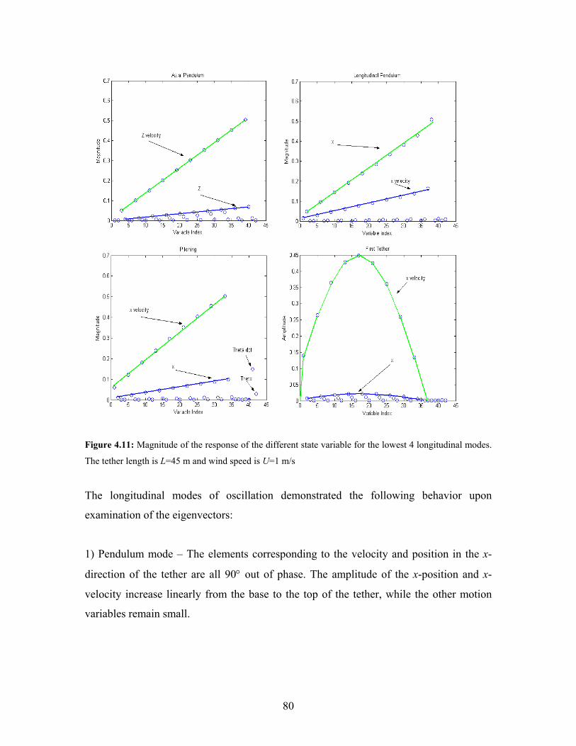
Figure 4.11: Magnitude of the response of the different state variable for the lowest 4 longitudinal modes.

The tether length is L=45 m and wind speed is U=1 m/s

The longitudinal modes of oscillation demonstrated the following behavior upon

examination of the eigenvectors:

1) Pendulum mode – The elements corresponding to the velocity and position in the x-

direction of the tether are all 90° out of phase. The amplitude of the x-position and x-

velocity increase linearly from the base to the top of the tether, while the other motion

variables remain small.

80

2) Pitching mode – The dominant motion of this mode is the pitching of the aerostat. The

magnitude of the x-position and the x-velocity of the tether are also appreciable which

suggests that the pitching motion is coupled with the x displacement of the tether. The

magnitude of x10 is negligible as expected since it corresponds to the centre of gravity

position about which the pitching rotation occurs.

3) Axial spring - The elements corresponding to the velocity and the position in the z-

direction are 90° out of phase. The amplitude of the z-positions and velocities increase

linearly from the base to the top of the tether. The dominant motion is in z with all other

variables being close to zero.

4) First tether mode– The elements corresponding to the position and velocity in the x-

direction of the tether nodes are all 90° out of phase. The magnitude of the x-position is a

maximum at the middle of the tether, corresponding to half of a sine cycle, which is

consistent with the definition of the fundamental frequency.

The 4 lowest lateral modes are classified in the same manner. The plots are not shown for

the sake of brevity but are similar to those of the corresponding longitudinal modes.

1) Pendulum mode – The elements corresponding to the velocity and the position in the

y-direction of the tether are all 90° out of phase. The amplitude of the y-position and

velocity increase linearly from the base to the top of the tether. The other motion

variables remain small.

2) Rolling mode – The dominant motion of this mode is the rolling of the aerostat. The

magnitudes of the y-position and of the y-velocity are also appreciable which suggests

that the pitching motion is coupled with the y displacement of the tether. The y10

magnitude is negligible as expected since it corresponds to the centre of gravity about

which the rolling rotation occurs.

81

3) First tether mode– The elements corresponding to the position and velocity in the y-

direction of the tether nodes are all 90° out of phase. The magnitude of the y-position is a

maximum at the middle of the tether, corresponding to half of a sine cycle, which is

consistent with the definition of the fundamental frequency.

4) Second tether mode- The y-position and velocity nodes are all 90° out of phase. The

motion of the first 5 nodes is 180° out of phase with that of the last 5 nodes. The

magnitude of the y-position has maximum at nodes 2 and 7 and minimum at node 5. This

corresponds to a full sine wave, which is characteristic of 1st tether harmonic.

To better understand these oscillations physically, a graphical interpretation of the

modes of oscillation is presented in Figure 4.12. The lateral pendulum is highlighted

since it has been shown from the experiment to strongly dominate the dynamics of the

system. The longitudinal pendulum and axial spring were also observed but their

response was much weaker.

z y

Figure 4.12: Graphical representation of the various modes of oscillation of a spherical tethered aerostat.

82

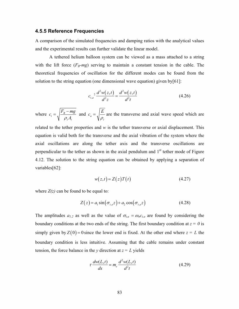
4.5.5 Reference Frequencies

A comparison of the simulated frequencies and damping ratios with the analytical values

and the experimental results can further validate the linear model.

A tethered helium balloon system can be viewed as a mass attached to a string

with the lift force (FB-mg) serving to maintain a constant tension in the cable. The

theoretical frequencies of oscillation for the different modes can be found from the

solution to the string equation (one dimensional wave equation) given by[61]:

( ) ( )2 22

, 2 2

, ,t a

d w z t d w z tc

d z d t= (4.26)

where Bt

t t

F mgcAρ

−= and a

t

Ecρ

= are the transverse and axial wave speed which are

related to the tether properties and w is the tether transverse or axial displacement. This

equation is valid both for the transverse and the axial vibration of the system where the

axial oscillations are along the tether axis and the transverse oscillations are

perpendicular to the tether as shown in the axial pendulum and 1st tether mode of Figure

4.12. The solution to the string equation can be obtained by applying a separation of

variables[62]:

( ) ( ) ( ),w z t Z z T t= (4.27)

where Z(z) can be found to be equal to:

( ) ( ) ( )1 , 2 ,sin cost a t aZ z a z a zσ σ= + (4.28)

The amplitudes a1,2 as well as the value of σt,a = ωnct,a are found by considering the

boundary conditions at the two ends of the string. The first boundary condition at z = 0 is

simply given by since the lower end is fixed. At the other end where z = L the

boundary condition is less intuitive. Assuming that the cable remains under constant

tension, the force balance in the y direction at z = L yields

( )0Z = 0

2

2

( , ) ( , )e

dw L t d w L tmdx d t

τ = (4.29)

83

where me is the aerostat equivalent mass including the added mass and τ is the tension in

cable. Using the boundary conditions at z = 0 and z = L and equation (4.26) the following

transcendental equation is derived:

,,

1 tant tt a

e t a

LA Lm L

ρ σσ

=

(4.30)

where t LAtρ is simply mt, the total mass of the tether. The solution ,t a Lσ can be obtained

graphically by plotting and finding the intersections of the right-hand side and left-hand

side of equation (4.30). The 5 lowest frequencies obtained analytically in the axial and

transverse directions are compared in Table 4.4 to the corresponding frequencies

extracted from the eigenvalues of the linear longitudinal and lateral analysis for a wind of

1 m/s. It is important to notice that for low wind speeds, the y (transverse to wind) and x

(along wind) direction of the spherical aerostat can be considered equivalent due to

symmetry. The analytical solution of the string equation do not consider the effect of the

wind and for the linear analysis, the 1 m/s wind speed was assumed close enough to a no

wind condition. Thus the frequencies shown in Table 4.4 for the transverse tether and

transverse pendulum mode apply equally well for oscilllations in the x and y directions.

Table 4.4: Comparison of the analytical and model modal frequencies for L = 45m

Analytical solution number

Corresponding mode name

Eigenvalue Simulated frequency ω (rad/s)

Theoretical frequency ω (rad/s)

Axial 5 Axial Tether 4th harmonic (long.) -0.015 ± 1743.2i 1743.2 1863.82

Axial 4 Axial Tether 3rd harmonic (long.) -0.021 ± 1346.4i 1346.4 1397.86

Axial 3 Axial Tether 2nd harmonic (long.) -0.018 ± 916.47i 916.5 931.91

Axial 2 Axial Tether fundamental (long.)

-0.027 ± 464.04i 464.0 465.95

Axial 1 Axial Pendulum (long.) -0.057 ± 7.3114i 7.31 7.28

Transverse 5

Transverse Tether 4th harmonic (long. and lat.)

-0.483 ± 78.798i 78.8 84.57

84

Transverse 4

Transverse Tether 3rd harmonic (long. and lat.)

-0.586 ± 60.87i 60.87 63.43

Transverse 3

Transverse Tether 2nd harmonic (long. and lat.)

-0.667 ± 41.451i 41.45 42.28

Transverse 2

Transverse Tether fundamental (long. and lat.)

-0.715 ± 21.038i 21.05 21.14

Transverse 1 Transverse Pendulum (long. and lat.)

-0.117 ± 0.298i 0.320 0.330

The various modes agree within 10% of the simulated value, and the lowest frequency

mode (which dominates the motion) is within 3%. One notes that transverse or axial

mode 2 frequency and onward can be approximated by

( )at

n Lcn

,

1 πω −= (4.31)

with n = 2,3,… Transverse or axial mode 1 is distinctly different from the others.

Transverse mode 1 is classically known as the pendulum mode while transverse modes 2

onward are the fundamental transverse tether vibration mode and its harmonics. The

pattern exhibited by the axial modes is the same as for the transverse vibrations. Axial

mode 1 can be thought of as an ‘axial pendulum’ mode, while axial modes 2 onward are

the fundamental axial mode and its harmonics.

These modes of oscillation were also observed experimentally, it was found that

the transverse pendulum was dominant and its frequency was within 30% of that

predicted. The axial spring mode was also observed in the spectral density of the tension

and its frequency was within 50% of the predicted one. The discrepancy can be attributed

to uncertainties in the tether properties. Figure 4.13 shows the spectral density of the

tension data for Flight 9, the dotted lines show the theoretical frequency as derived above.

For the tether length L = 15m, the axial pendulum mode seems absent in the experimental

results.

85

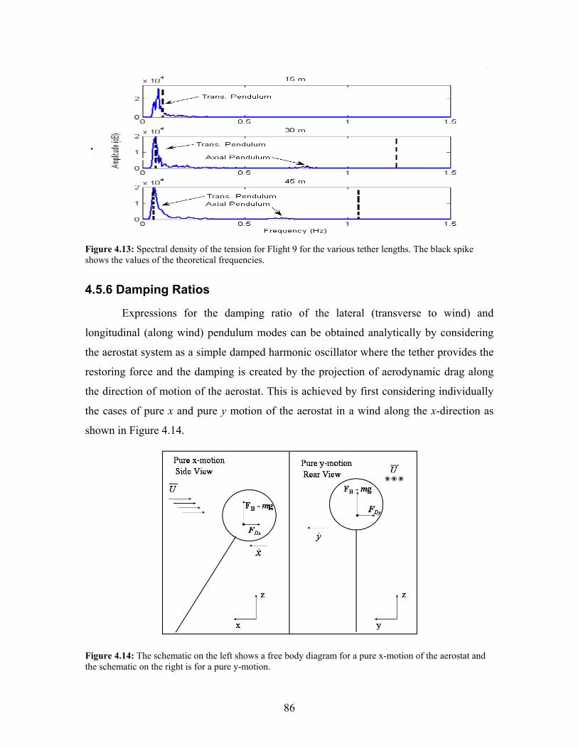
Figure 4.13: Spectral density of the tension for Flight 9 for the various tether lengths. The black spike shows the values of the theoretical frequencies.

4.5.6 Damping Ratios

Expressions for the damping ratio of the lateral (transverse to wind) and

longitudinal (along wind) pendulum modes can be obtained analytically by considering

the aerostat system as a simple damped harmonic oscillator where the tether provides the

restoring force and the damping is created by the projection of aerodynamic drag along

the direction of motion of the aerostat. This is achieved by first considering individually

the cases of pure x and pure y motion of the aerostat in a wind along the x-direction as

shown in Figure 4.14.

Figure 4.14: The schematic on the left shows a free body diagram for a pure x-motion of the aerostat and the schematic on the right is for a pure y-motion.

86

From the free body diagram of Figure 4.14, the equation of motion for the pure x-motion

of the aerostat can be formulated as

Dxxe Fxkxm =+&& (4.32)

and for pure y-motion as

Dyye Fykym =+&& (4.33)

where ( ),

Bx y

F mgk

L−

= is the restoring force coefficient and; FDy and FDx are

respectively the x and y horizontal projection of the drag force FD. In order to obtain

expressions for the damping coefficient, equations (4.32) and (4.33) have to be expressed

in a linear form. This is achieved by expressing FDx and FDy as function of x& and and

linearizing the resulting relations. The first thing to note is that the aerodynamic drag

force expressed as

y&

212D a D rF ACρ= elU (4.34)

always acts along the direction of the relative velocity Urel and therefore the direction of

FD is known. According to Figure 4.14 for a pure x-motion of the aerostat, is

formulated in component form as

relU

0 0T

U x = − relU & (4.35)

and for a pure y-motion of the aerostat as

0T

U y = − relU & (4.36)

Now, the norm of the relative velocity is expressed from equations (4.35) and (4.36) as:

2 2rel

U x pure x motionU

U y pure y motion

−= +

&

& (4.37)

For the case of pure x-motion, an expression for the x-projection of the drag force FDx is

obtained from equations (4.34) and (4.37) and by noting from equation (4.35) that FDx =

FD:

87

( )212Dx DF AC Uρ= &x− (4.38)

For the case of pure y-motion, an expression for of the y-projection of the drag force FDy

can be obtained from equations (4.34) and (4.37) and using equation (4.36):

( )1

2 2 212Dy D D

rel

yF F AC y U yU

ρ= = +&

& & (4.39)

Now linearizing expressions (4.38) and (4.39) respectively about x& = 0 and = 0 and

putting the results back in right-hand-side of equations (4.32) and (4.33) we obtain two

linear second order differential equations in x and y:

y&

2

1

22

nx x

ny y

x x x C for pure x motion

y y y C for pure y motion

ω κ

ω κ

+ + = −

+ + = −

&& &

&& & (4.40)

where C1,2 are constants, ,2,

x ynx y

e

km

ω = and the damping terms ,x yκ is related to the

damping ratio ζx,y by

2

22

D ax x n

e

D ay y n

e

C AUm

C AUm

ρκ ζ ω

ρκ ζ ω

= =

= = (4.41)

The values of the theoretical and simulated damping ratio for the transverse pendulum

mode’s x motion and y motion of the aerostat with L = 45m and U = 1 m/s are presented

in Table 4.5

Table 4.5: Comparison of the simulated and theoretical damping ratio for U=1m/s and L=45m

Simulated Value Theoretical Value

Damping ratio along

wind xζ 0.37 0.36

Damping ratio

perpendicular to wind

yζ 0.l8 0.18

88

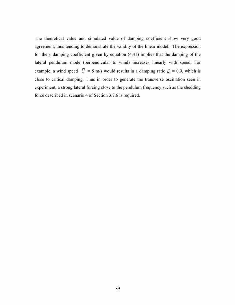
The theoretical value and simulated value of damping coefficient show very good

agreement, thus tending to demonstrate the validity of the linear model. The expression

for the y damping coefficient given by equation (4.41) implies that the damping of the

lateral pendulum mode (perpendicular to wind) increases linearly with speed. For

example, a wind speed U = 5 m/s would results in a damping ratio ζy = 0.9, which is

close to critical damping. Thus in order to generate the transverse oscillation seen in

experiment, a strong lateral forcing close to the pendulum frequency such as the shedding

force described in scenario 4 of Section 3.7.6 is required.

89

Chapter 5

Conclusion

5.1 Test Facility

The design and construction of a portable experimental set-up for the characterization of

the dynamics of tethered aerostat was successfully achieved. The set-up has been used to

record the dynamics variables of a tethered spherical aerostat and the concept could

easily be applied to other types of helium balloons.

The 3.5m spherical aerostat purchased from Aerostar was shown to be reliable

and low maintenance; the helium lost per day was minor. A diameter of 1.5 mm was

picked for the tether diameter to respect a factor of safety of three on breaking strength.

The wind gusts seen in experiment were larger than expected and a tether diameter of

1.75-2.0 mm is recommended. At the confluence point, the main line was divided into

four secondary lines attached to straps on the aerostat. This configuration was found to

efficiently reduce stress concentrations on the balloon. The winch used was lightweight

and battery powered; and these features were highly appreciated for field

experimentation. However, it was found to be a bit slow to retrieve the balloon in high

wind (about 5-10 m/min).

The instrumentation platform carrying the sensors was proven to be reliable and

was well secured to the balloon throughout the flights. The use of stabilization lines

going from the platform to the aerostat straps helped to reduce the relative motion of the

platform with respect to the aerostat.

The sensors are divided in three groups: the position sensors, the tension sensors

and the wind sensors. After differential post-processing of the GPS data using GrafNav

software from WayPoint consulting, an accuracy of 5 cm at a rate of 10 Hz was achieved

90

on position. The tension acquisition system performed poorly, mainly because of the

signal conditioner board. The wind speed and direction sensors were found to be reliable,

but had relatively low bandwidth.

The communication software was an efficient tool to acquire and synchronise the

sensors’ data. However, the radio link, communicating with airborne sensors, sometimes

failed during a flight due to the poor performance of the virtual serial ports.

The experimental set-up was found to be compliant with all the requirements set

in Section 2.1.

5.2 Data Analysis

A total of nine flights were performed. For most of these flights, the aerostat was flown

at tether lengths of 15, 30 and 45m. The time history of the position and of the tension, as

well as the wind speed and direction were recorded. The free lift of the aerostat was

measured to be 136.5 N.

The wind speeds and directions were measured at 3, 5 and 10m. In order to get the

mean wind speed at the aerostat height, a power law relationship was used. The power m

was found to vary from 0.11 to 0.14, depending on the day of acquisition. Typical mean

wind speed at the balloon height varied from 2 to 7 m/s. These wind speeds are all in the

supercritical regime of flow for our system.

The mean drag coefficient CD of the tethered sphere was determined using a

quasi-static approximation. An average CD of 0.56 was calculated that is, three times

higher than for a fixed sphere at supercritical Reynolds numbers. The CD value of the

aerostat is consistent with Williamson’s result for a tethered sphere in the same reduced

velocity range but at much lower Reynolds number [29]. This might suggest that the

supercritical drop for a tethered sphere is small compared to a fixed sphere. The CD value

of our system has been shown to be only slightly lower than that of a rough free buoyant

sphere (not attached to ground) [24].

Williamson et al. have shown that a tethered sphere in uniform flow would tend

to oscillate both in the streamwise and transverse directions. Our experiment

demonstrated that this behaviour is also true for a tethered sphere in a turbulent flow

field. However, the streamwise oscillations are less evident, probably due to wind speed

91

and direction variations. The transverse oscillations of the aerostat were characterized by

plotting the normalized amplitudes A* with reduced velocity. It was found that the

amplitude of transverse oscillations increased with reduced velocity and that the

normalized amplitude is independent of tether length. Our normalized amplitudes match

reasonably well those of Williamson for the lower reduced velocity (5-10) range

however, they do not exhibit the saturation in amplitude of A*=1 at reduced velocities

higher than 13 [29].

A FFT of the y motion demonstrated that the transverse oscillations occur within

30 % of the aerostat pendulum frequency. This result is consistent with Williamson’s

result for a tethered sphere in the same reduced velocity regime and similar mass ratio. It

suggests that there is a periodic force or component of force acting transversely on the

aerostat close the natural frequency.

The classical theory explains the transverse oscillations by a lock-in of the

principal component of the vortex shedding frequency with the system oscillation

frequency [32]. This explanation does not apply to our system since all our experiments

were performed in the supercritical regime of flow where there is no definite frequency in

the wake of a fixed sphere [21].

The most plausible explanation for the strong oscillations observed

experimentally is that they result from a ‘movement induced excitation’. The oscillations

are generated by self-sustaining vortex force generated by the motion of the tethered

sphere. Govardhan and Williamson have shown that this phenomenon happens for

tethered spheres in the reduced velocity range of 8 to 40, which is squarely in the range

of our experiment [32].

5.3 Simulation

The dynamic analysis of the tethered spherical aerostat was based on a prior model

created by Lambert [4]. The effects of the experimental platform on the system were

taken into account using a combination of measurements and CAD model calculations.

The equations of motion of the aerostat were derived including the offset of the CG due

to the experimental platform. This resulted in the addition of the three rotational

92

equations of motion. A revised wind model was proposed to account for the type of

terrain and altitude at which the experiments were performed.

A transverse sinusoidal force applied at the aerostat’s CG was included to

represent the ‘movement-induced excitation’ conjectured by Govardhan and Williamson.

The amplitude of the force was related to the amplitude of the motion up to a saturating

value of 27.7 N. This amplitude was derived from direct force measurement obtained by

Williamson on a tethered sphere in the same reduced velocity range.

An attempt to validate the non-linear dynamics simulation was made by

comparing the model output to experimental results of three flight sections. It was shown

that the simulation is in good agreement with the experiment for the three flights. The x-

motion of the aerostat exhibited very similar behaviour in experiment and in simulation.

The transverse oscillations of the aerostat were found to be smaller in simulation than in

reality. This might suggest that the lateral vortex force is slightly larger for our system

than predicted by Williamson’s results. The experimental z-motion and the tension show

large peaks, which are not present in the simulation results. This discrepancy might be

explained by an underestimation of the z-gust component of the wind turbulence.

A numerical linearization of the system’s equations of motion was performed.

The properties of the resulting state matrix indicates that the aerostat motion can be split

into longitudinal and lateral motions. The eigenvalues and eigenvectors of the state

matrix were used to characterize the behaviour of the system into oscillatory modes. The

frequencies of the four lowest modes of oscillation were compared to corresponding

frequencies obtained analytically and excellent agreement was observed. This further

validates the dynamics model. An analytical expression for the damping ratio of the

streamwise and lateral pendulum mode was also obtained, and shown to be in excellent

agreement with the linear model. The damping of the pendulum mode was found to be

very high, which suggests that the lateral oscillations seen in the experiment are caused

by strong forcing at that frequency as conjectured by Govardhan and Williamson.

93

5.4 Recommendations

The following recommendations pertain to the experimental system:

New spherical balloon designs could be investigated to reduce the drag coefficient

and the amplitude of the aerostat lateral oscillations. A splitter plate behind the

sphere would be one suggestion for achieving this.

Add instrumentation to record the accelerations of the balloon. This would allow

for an instantaneous analysis of the system as well as the measurement of the time

history of the drag and lift forces.

Add a wind sensor close to the balloon. This could allow for a time history

comparison of the simulated and experimental dynamics variables.

The following recommendations pertain to the simulation:

Further investigate the phenomenon that generates the lateral oscillations of the

aerostat. This would necessitate further study of tethered sphere behaviour in fluid

flow especially at high reduced velocity and high Re.

Further investigate the z-component of the wind gust. This would help to

understand the spikes observed in the z-position and tension data.

94

References

1. Picture of the first demonstrated flight available at www.eballoon.org. 2. Picture of the explosion of the Hindenburg available at www.nyt-

gallery.myfoto.de. 3. Picture of a streamlined aerostat available at www2.acc.af.mil. 4. Lambert, C.M., Dynamics Modeling and Conceptual Design of Multi-tethered

Aerostat System, in Mechanical Engineering. 2002, Universtiy of Victoria: Victoria. p. 158.

5. Jones, S.P., A Stability Analysis for Tethered Aerodynamically Shaped Balloons. AIAA Journal of Aircraft, 1972. 9(9): p. 646-651.

6. Redd, T., R. Bland, and R.M. Bennet, Stability Analysis and Trend Study of a Balloon Tethered in a Wind, With Experimental Comparisons. NASA TN D-7272, 1973: p. 1-109.

7. Jones, S.P. and J.A. Krausman, Nonlinear Dynamic Simulation OF A Tethered Aerostat. 1982. 19(8): p. 679.

8. Jones, S.P. and J.D. DeLaurier, Aerodynamic Estimation Techniques for Aerostat and Airships. AIAA Journal of Aircraft, 1983. 20(2): p. 120-126.

9. Nahon, M., Dynamics and Control of a Novel Radio Telescope Antenna. A Collection of the AIAA Modeling and Simulation Technologies Conference Technical Papers, 1999: p. 214-222.

10. Nahon, M., A Simplified Dynamics Model for Autonomous Underwater Vehicles. IEEE Proceedings of AUV'96, 1996: p. 373-379.

11. R.Driscoll, M.N., Mathematical Modeling and Simulation of Moored Buoy System. Proceedings of Oceans, 1996: p. 517-523.

12. Buckham, B., et al., Dynamics and control of a towed underwater vehicle system, part I: Model development. Ocean Engineering, 2002. 30(4): p. 453.

13. Jones, S.P. and L.D. Schroeder, Nonlinear dynamic simulation of a tethered aerostat: A fidelity study. Journal of Aircraft, 2001. 38(1): p. 64.

14. Lambert, C. and M. Nahon, Stability analysis of a tethered aerostat. AIAA Journal of Aircraft, 2003. 40(4): p. 705.

15. Stanney, K.A. and C.D. Rahn. Response of a tethered aerostat to simulated turbulence. 2004. Anaheim, CA, United States: American Society of Mechanical Engineers, New York, NY 10016-5990, United States.

16. Lambert, C.M. and M. Nahon, Study of a Multi-tethered Aerostat System - Experimental Observations and Model Validation. submitted to AIAA Journal of Aircraft, 2005.

95

17. Dewdney, P., M. Nahon, and B. Veidt, The large adaptive reflector: A giant radio telescope with an aero twist. Canadian Aeronautics and Space Journal, 2002. 48(4): p. 239.

18. Sakamoto, H. and H. Haniu, A Study of Vortex Shedding From Spheres in a Uniform Flow. Journal of Fluid Engineering, 1990. 112: p. 386-392.

19. Achenbach, E., Experiments on the Flow Past Spheres at Very High Reynolds Number. Journal of Fluid Mechanics, 1972. 54(3): p. 565-575.

20. Taneda, S., Visual Observations of the Flow Past a Sphere at Reynolds Numbers Between 10^4 and 10^6. 1978. 85(1): p. 192.

21. Willmarth, W.W. and R.L. Enlow, Aerodynamic Lift and Moment Fluctuations of a Sphere. Journal of Fluid Mechanics, 1969. 36(3): p. 417-432.

22. Howe, M.S., G.C. Lauchle, and J. Wang, Aerodynamic lift and drag fluctuations of a sphere. Journal of Fluid Mechanics, 2001. 436: p. 41.

23. Scoggins, J.R., Spherical balloon wind sensor behavior. Journal of Applied Meteorology, 1965. 4(1): p. 139.

24. Scoggins, J.R., Sphere Behavior and the Measurement of Wind Profile. NASA TN D-3994, 1967: p. 1-53.

25. Kruchinin, N.N., Transverse Oscillations of Pendulous Sphere in a Flow. Moscow Mechanics Bulletin (English Translation of Vestnik Moskovskogo Universiteta, Mekhanika), 1977. 32(3-4): p. 8-13.

26. Harleman, D.R.F. and W.C. Shapiro, The Dynamics of a Submerged Moor Sphere in Oscillatory Waves. Coastal Engineering, 1961. 2: p. 746-765.

27. Shi-Igai, H. and T. Kono, Study on Vibration of Submerged Spheres Caused by Surface Waves. Coastal Engineering in Japan, 1969. 12: p. 29-40.

28. Ogihara, K., Theoretical Analysis on the Transverse Motion of a Buoy by a Surface Wave. Applied Ocean Research, 1980. 2: p. 51-56.

29. Williamson, C.H.K. and R. Govardhan, Dynamics and Forcing of a Tethered Sphere in a Fluid Flow. Journal of Fluids and Structures, 1997. 11(3): p. 293.

30. Govardhan, R. and C.H.K. Williamson, Vortex-Induced Motions of a Tethered Sphere. Journal of Wind Engineering and Industrial Aerodynamics, 1997. 69-71: p. 375.

31. N.Jauvtis, R.Govardhan, and C.H.K. Williamson, Multiple Modes of Vortex-Induced Vibration of a Sphere. Journal of Fluid and Structures, 2001. 15: p. 555-563.

32. Govardhan, R.N. and C.H.K. Williamson, Vortex-induced vibrations of a sphere. Journal of Fluid Mechanics, 2005. 531: p. 11.

33. E.Naudasher and D.Rockwell, Flow Induced Vibrations: An Engineering Guide. Balkema ed. 1994.

34. Bearman, P.W., Vortex Shedding from Oscillating Bluff Bodies. Annual Review of Fluid Mechanics, 1984. 16: p. 195.

35. Anagnostopoulos, P., Flow-induced vibrations in engineering practice. 2002, Southampton; Boston: WIT Press. 388.

36. Picture of the TIF-460 aerostat from Aerostar available at www.aerostar.com. 37. Picture of the Skydoc® aerostat from FLOATOGRAPH available at

www.floatograph.com. 38. Picture of the Helikite® aerostat from ALLSOPP available at www.allsopp.co.uk.

96

39. Aerostar streamlined and spherical aerostat properties available at www.aerostar.com.

40. McCormick, B.W., Aerodynamics, Aeronautics and Flight Mechanics. 1995. 41. Goldstein, S. and Aeronautical Research Council (Great Britain), Modern

developments in fluid dynamics: an account of theory and experiment relating to boundary layers, turbulent motion and wakes. 1965, New York: Dover Publications. 2 v. (xxviii, 702, 35 leaves of plates).

42. Schlichting, H., Boundary Layer Theory. 7 ed. 1979, New York: McGraw-Hill. 43. Pudget Sound Rope PLASMA 12 Strand data sheer available at www.psrope.com. 44. Hofmann-Wellenhof, B., H. Lichtenegger, and J. Collins, Global Positioning

System: theory and practice. 5th, rev. ed. 2001, Wien; New York: Springer-Verlag. xxii, 382.

45. 05103-10 R.M. Young Wind Monitor Instruction Manual. 1984-1996, Campbell Scientific. p. 1-15 available at www.campbellsci.ca.

46. Hiriart, D., J.L. Ochoa, and B. Garcia, Wind Power Spectrum Measured at the San Pedro Martir Sierra. Revista Mexicana de Astronomia y Astrofisica, 2001. 37: p. 213-220.

47. Houblot, J.C., Atmospheric Turbulence. AIAA Journal, 1973. 11(4): p. 421-437. 48. Guyot, G., Physics of the Environment and Climate. Praxis ed. 1998, Toronto:

Wiley and Sons. 632. 49. Stull, R.B., An Introduction to Boundary Layer Meteorology. 1988: Kluwer

Academic Press. 666. 50. Wieselsberger, C.v., Weitere Festllungen uber dei Geset des Flussigkeits un

Luftwiderstandes. Physikalische Zeitschrift, 1922. 23: p. 219-224. 51. Govardhan, R. and C.H.K. Williamson, Resonance Forever: Existence of a

Critical Mass and an Infinite Regime of Resonnance in Vortex-Induced Vibration. Journal of Fluid Mechanics, 2002. 473: p. 147-166.

52. Ryan, K., et al., Flow-Induced Vibration of a Tethered Circular Cylinder. Journal of Fluid and Structures, 2004. 19: p. 1085-1102.

53. Jauvtis, N., R. Govardhan, and C.H.K. Williamson, Multiple Modes of Vortex-Induced Vibration of a Sphere. Journal of Fluid and Structures, 2001. 15: p. 555-563.

54. Nahon, M., G. Gilardi, and C. Lambert, Dynamics/control of a radio telescope receiver supported by a tethered aerostat. Journal of Guidance, Control, and Dynamics, 2002. 25(6): p. 1107.

55. Lambert, C., et al., Dynamics and control of towed underwater vehicle system, part II: Model validation and turn maneuver optimization. Ocean Engineering, 2002. 30(4): p. 471.

56. Newman, J.N., Marine Hydrodynamics. 1989: MIT Press. 57. Etkin, B. and L.D. Reid, Dynamics of flight: stability and control. 3rd ed. 1996,

New York: Wiley. xi, 382. 58. Engineering Sciences Data Unit., E.S.D.U.CCharacteristics of Atmospheric

Turbulence Near the Ground, 1974, Item Number 74031 59. Etkin, B., Stability of a Towed Body. AIAA Journal of Aircraft, 1998. 35(2): p.

197-205.

97

98

60. Ogata, K., System dynamics. 4th ed. 2004, Upper Saddle River, NJ: Pearson/Prentice Hall. ix, 768.

61. Inman, D.J., Engineering Vibration. 2nd ed. 2001, Upper Saddle River,NJ: Pearson/Prentice Hall, 621.

62. Haberman, R., Elementary Applied Partial Differential Equations. 3 ed. 1983, Upper Saddle River: Prentice Hall. 736.