Simulating Zeno Hybrid Systems Beyond Their Zeno Points · Simulating Zeno Hybrid Systems Beyond...
47
Simulating Zeno Hybrid Systems Beyond Their Zeno Points Haiyang Zheng Electrical Engineering and Computer Sciences University of California at Berkeley Technical Report No. UCB/EECS-2006-114 http://www.eecs.berkeley.edu/Pubs/TechRpts/2006/EECS-2006-114.html September 8, 2006
Transcript of Simulating Zeno Hybrid Systems Beyond Their Zeno Points · Simulating Zeno Hybrid Systems Beyond...

Simulating Zeno Hybrid Systems Beyond Their ZenoPoints
Haiyang Zheng
Electrical Engineering and Computer SciencesUniversity of California at Berkeley
Technical Report No. UCB/EECS-2006-114
http://www.eecs.berkeley.edu/Pubs/TechRpts/2006/EECS-2006-114.html
September 8, 2006

Copyright © 2006, by the author(s).All rights reserved.
Permission to make digital or hard copies of all or part of this work forpersonal or classroom use is granted without fee provided that copies arenot made or distributed for profit or commercial advantage and that copiesbear this notice and the full citation on the first page. To copy otherwise, torepublish, to post on servers or to redistribute to lists, requires prior specificpermission.

Simulating Zeno Hybrid Systems Beyond Their Zeno Points
by Haiyang Zheng
Research Project
Submitted to the Department of Electrical Engineering and Computer Sciences,
University of California at Berkeley, in partial satisfaction of the requirements for
the degree of Master of Science, Plan II.
Approval for the Report and Comprehensive Examination:
Committee:
Professor Edward A. Lee
Research Advisor
Date
* * * * * *
Professor Shankar Sastry
Second Reader
Date

ii

Contents
Contents ii
Acknowledgements v
Abstract vi
1 Introduction 1
1.1 Bouncing Ball . . . . . . . . . . . . . . . . . . . . . . . . . . . . . . . 3
1.2 Water Tank . . . . . . . . . . . . . . . . . . . . . . . . . . . . . . . . 5
2 Completing Hybrid Systems 9
2.1 Hybrid System Completion . . . . . . . . . . . . . . . . . . . . . . . . 9
2.2 Examples . . . . . . . . . . . . . . . . . . . . . . . . . . . . . . . . . 18
2.2.1 Example 1: Bouncing Ball. . . . . . . . . . . . . . . . . . . . . 18
2.2.2 Example 2: Water Tank. . . . . . . . . . . . . . . . . . . . . . 21
2.2.3 Example 3: A Non-Zeno Hybrid System. . . . . . . . . . . . . 23
2.2.4 Example 4: A Zeno Hybrid System. . . . . . . . . . . . . . . . 25
2.2.5 Example 5: Another Zeno Hybrid System. . . . . . . . . . . . 26
3 Approximate Simulation 29
3.1 Numerical Errors . . . . . . . . . . . . . . . . . . . . . . . . . . . . . 30
3.2 Computation Difficulties . . . . . . . . . . . . . . . . . . . . . . . . . 31
3.3 Approximating Zeno Behaviors . . . . . . . . . . . . . . . . . . . . . 33
3.3.1 Issue 1: Relaxing Guard Expressions. . . . . . . . . . . . . . . 34
3.3.2 Issue 2: Reinitialization. . . . . . . . . . . . . . . . . . . . . . 35
iii

4 Conclusion 37
bibliography 38
References . . . . . . . . . . . . . . . . . . . . . . . . . . . . . . . . . . . . 38
iv

Acknowledgements
This work was supported in part by the Ptolemy project, the Center for Hybrid
and Embedded Software Systems (CHESS) at UC Berkeley, which receives support
from the National Science Foundation (NSF award #CCR-0225610), the State of
California Micro Program, and the following companies: Agilent, DGIST, General
Motors, Hewlett Packard, Infineon, Microsoft, and Toyota.
I would like to thank Aaron D. Ames. Much of the work presented in this report
is collaborated with Aaron. He gives me a lot of useful and constructive comments
and discussions on Zeno hybrid systems. His passion on Zeno hybrid systems greatly
motivates the work presented in this report. Any errors appearing in this report are
of my sole responsibility.
I would like to thank Adam Cataldo for helping me on the concepts of compact
and closed sets. I would like to thank Jonathan Sprinkle for his kindness and patience
on helping me about Latex questions. I would also like to thank the whole Ptolemy
group for their feedback.
This report is dedicated to my parents and extended family. This report is in
memory of my grandpa.
v

Abstract
In this report a technique is proposed to extend the simulation of a Zeno hybrid
system beyond its Zeno time point. A Zeno hybrid system model is a hybrid system
with an execution that takes an infinite number of discrete transitions during a finite
time interval. Some classical Zeno models that incompletely describe the dynamics
of the system being modeled are revisited to show that the presence of Zeno behavior
indicates that the hybrid system model is incomplete. This motivates the systematic
development of a method for completing hybrid system models through the introduc-
tion of new post-Zeno states, where the completed hybrid system transitions to these
post-Zeno states at the Zeno time point.
In practice, simulating a Zeno hybrid system is challenging in that simulation
effectively halts near the Zeno time point. Moreover, due to unavoidable numerical
errors, it is not practical to exactly simulate a Zeno hybrid system. Therefore, a
method for constructing approximations of Zeno models by leveraging the completed
hybrid system model is proposed. Using these approximation, a Zeno hybrid system
model can be simulated beyond its Zeno point and so the complete dynamics of the
system being modeled is revealed.
vi

Chapter 1
Introduction
The dynamics of physical systems at the macro scale level (not considering ef-
fects at the quantum level) are continuous in general. Even in a digital computer
that performs computation in a discrete fashion, its fundamental computing elements
(transistors) have continuous dynamics. Therefore, it is a natural choice to model the
dynamics of physical systems with ordinary differential equations (ODEs) or partial
differential equations (PDEs). However, modeling a physical system with only contin-
uous dynamics may generate a stiff model, because the system dynamics might have
several time scales of different magnitudes. Simulating such stiff models in general
is difficult in that it takes a lot of computation time to get a reasonably accurate
simulation result.
Hybrid system modeling offers one way to resolve the above problem by introduc-
ing abstractions on dynamics. In particular, slow dynamics are modeled as piecewise
constants (at different phases) while fast dynamics are modeled as instantaneous
changes, i.e., discretely. In this way, the remaining dynamics will have time scales of
about the same magnitude and the efficiency of simulation, especially the simulation
1

speed, is greatly improved. However, special attention must be devoted to hybrid
system models because Zeno hybrid system models may arise from the abstractions.
An execution of a Zeno hybrid system has an infinite number of discrete transitions
during a finite time interval. The limit of the set of switching time points of a Zeno
execution is called the Zeno time. The states of the model at the Zeno time point are
called the Zeno states. Because each discrete transition takes a non-zero and finite
computation time, the simulation of a Zeno hybrid system inevitably halts near the
Zeno time point.
Some researchers have treated Zeno hybrid system models as over abstractions of
the physical systems and tried to rule them out by developing theories to detect Zeno
models [1]–[3]. However, because of the intrinsic complexity of interactions between
continuous and discrete dynamics of hybrid systems, a general theory, which can give
the sufficient and necessary conditions for the existence of Zeno behaviors of hybrid
system models with nontrivial dynamics, is still not available (and does not appear
to be anywhere on the horizon).
Some researchers have tried to extend the simulation of Zeno systems beyond the
Zeno point by regularizing the original system [4], [5] or by using a sliding mode
simulation algorithm [6]. The regularization method requires modification of the
model structure by introducing some lower bound of the interval between consecutive
discrete transitions. However, the newly introduced lower bound invalidates the ab-
stractions and assumptions of the instantaneity of discrete transitions. Consequently,
the simulation performance might suffer from the resulting stiff models. Furthermore,
different behaviors after the Zeno time may be generated depending on the choices of
regularizations. This may not be desirable because the physical system being mod-
eled typically has a unique behavior. The sliding mode algorithm tends to be more
2
promising in simulation efficiency and uniqueness of behaviors, but it only applies to
special classes of hybrid system models.
A new technique to extend simulations beyond the Zeno time point is presented
in [7], where a special class of hybrid systems called Lagrangian hybrid systems are
considered. Rather than using regularizations or a sliding mode algorithm, the dy-
namics of a Lagrangian hybrid system before and after the Zeno time point are derived
under different constraints. In this report, we extend the results in [7] to more general
hybrid system models.
Before we get into the details of the algorithm on extending simulation beyond
Zeno time points, we would like to investigate some classical Zeno hybrid system
models including the bouncing ball model [8] and the water tank model [4], and show
that they do not completely describe the behavior of the original physical systems.
1.1 Bouncing Ball
22 : xex ⋅−=00 21 ≤∧= xx
01 ≥x
gx
xx
−==
2
21
&
&
1q 1e
22 : xex ⋅−=00 21 ≤∧= xx
01 ≥x
gx
xx
−==
2
21
&
&
1q 1e
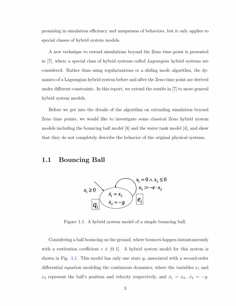
Figure 1.1. A hybrid system model of a simple bouncing ball.
Considering a ball bouncing on the ground, where bounces happen instantaneously
with a restitution coefficient e ∈ [0, 1]. A hybrid system model for this system is
shown in Fig. 1.1. This model has only one state q1 associated with a second-order
differential equation modeling the continuous dynamics, where the variables x1 and
x2 represent the ball’s position and velocity respectively, and x1 = x2, x2 = −g.
3

From this one state, there is a transition e1 that goes back to itself. The transition
has a guard expression, x1 = 0 ∧ x2 ≤ 0, and a reset map, x2 := −e · x2.1
22 : xex ⋅−=00 21 <∧= xx
01 ≥x
02
21
==
x
xx
&
&
00 21 =∧= xxgx
xx
−==
2
21
&
&
1q
1e2q
2e
22 : xex ⋅−=00 21 <∧= xx
01 ≥x
02
21
==
x
xx
&
&
00 21 =∧= xxgx
xx
−==
2
21
&
&
1q
1e2q
2e
Figure 1.2. A more complete hybrid system model of the bouncing ball.
Note that the above guard expression declares that a bounce happens when the
ball touches the ground and its velocity x2 is non-positive, meaning either it is still
or it is moving towards the ground. However, further analysis of the model reveals
that when the following condition holds, x1 = 0 ∧ x2 = 0, meaning that the ball is
at rest on the ground, the supporting force from the ground cancels out the gravity
force. Therefore, the acceleration of the ball should be 0 rather than the acceleration
of gravity. Under this circumstance, the ball in fact has a rather different dynamics
given by x1 = x2, x2 = 0.
This suggests that new dynamics might be necessary to describe the model’s
behavior. Consequently, the complete description of the dynamics of the bouncing
ball system should include both an extra state associated with the new dynamics and
a transition that drives the model into that state. One design of such a hybrid system
model is shown in Fig. 1.2, where q2 and e2 are the new state and transition.
1Identity reset maps, such as x1 := x1, are not explicitly shown.
4
1.2 Water Tank
The second model that we will consider is the water tank system consisting of two
tanks. We use x1 and x2 for the water levels, r1 and r2 for the critical water level
thresholds, and v1 and v2 for the constant flow of water out of the tanks. There is a
constant input flow of water w, which goes through a pipe and into either tank at any
particular time point. We assume that (v1 + v2) > w, meaning that the sum of the
output flow in both tanks is greater than the input flow. Therefore, the water levels
of both tanks keep dropping. If the water level of any tank drops below its critical
threshold, the input water gets delivered into that tank. The process of switching the
pipe from one tank to the other takes zero time.
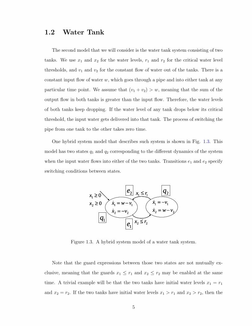
One hybrid system model that describes such system is shown in Fig. 1.3. This
model has two states q1 and q2 corresponding to the different dynamics of the system
when the input water flows into either of the two tanks. Transitions e1 and e2 specify
switching conditions between states.
0
0
2
1
≥≥
x
x
22
11
vwx
vx
−=−=
&
&
22 rx ≤
11 rx ≤
22
11
vx
vwx
−=−=
&
&
1q1e
2q2e
0
0
2
1
≥≥
x
x
22
11
vwx
vx
−=−=
&
&
22 rx ≤
11 rx ≤
22
11
vx
vwx
−=−=
&
&
1q1e
2q2e
Figure 1.3. A hybrid system model of a water tank system.
Note that the guard expressions between those two states are not mutually ex-
clusive, meaning that the guards x1 ≤ r1 and x2 ≤ r2 may be enabled at the same
time. A trivial example will be that the two tanks have initial water levels x1 = r1
and x2 = r2. If the two tanks have initial water levels x1 > r1 and x2 > r2, then the
5
water levels of both tanks will drop and the water pipe will switch between the two
tanks. As more and more water flows out of tanks, we will see that the frequency
of the pipe switching becomes higher and higher. In the limit, when this frequency
reaches infinity, both guards become enabled at the same time.
When both guards are enabled, the water tank system will have a different dy-
namics. Recall the assumption that the switching speed of the water pipe is infinitely
fast, the pipe should inject water into both tanks at the same time. In other words,
there are virtually two identical pipes injecting water into both tanks. Also note
that the input water flow is a constant and the pipe cannot hold water, therefore one
possible scenario will be that each tank gets half of the input water. Therefore, at
this time point, the whole system will have a rather different dynamics given by
x1 = w/2− v1, x2 = w/2− v2. (1.1)
We introduce a new state associated with the above dynamics and complete the
transitions going from the existing states to the newly added state. The new design
of the complete hybrid system model for the water tank system is shown in Fig. 1.4,
where q3 is the new state, e3 and e4 are the newly added transitions. Note that for
simplicity we allow the water levels to have negative values. Otherwise, we will need
some other discrete states to show that once a tank is empty, it is always empty.
The hybrid system model in Fig. 1.4 is similar to the temporal regularization
results proposed in [4]. One of the key differences is that the temporal regularization
solution requires the process of switching pipe to take some positive time ε. The
amount of this ε affects the resulting behaviors. In fact, when ε goes to 0, the
temporal regularization result is the same as what we have derived in (1.1).
In the next chapter, we will propose a systematic way to complete the specification
of hybrid system models. In particular, we will discuss how to introduce new states,
to modify the existing transitions, and to construct new transitions to these new
6

0
0
2
1
≥≥
x
x
22
11
vwx
vx
−=−=
&
&2211 rxrx >∧≤
22
11
2
2
vwx
vwx
−=−=
&
&
2211 rxrx ≤∧≤2211 rxrx ≤∧≤
1122 rxrx >∧≤22
11
vx
vwx
−=−=
&
&
1q1e
2q2e
3q3e
4e
0
0
2
1
≥≥
x
x
22
11
vwx
vx
−=−=
&
&2211 rxrx >∧≤
22
11
2
2
vwx
vwx
−=−=
&
&
2211 rxrx ≤∧≤2211 rxrx ≤∧≤
1122 rxrx >∧≤22
11
vx
vwx
−=−=
&
&
1q1e
2q2e
3q3e
4e
Figure 1.4. A more complete hybrid system model of the water tank system.
states for model behaviors before and after potential Zeno time points. In Chapter
3, we will develop a feasible simulation algorithm to approximate the exact behaviors
of Zeno hybrid system models. Conclusions will be given in Chapter 4.
7

8

Chapter 2
Completing Hybrid Systems
The purpose of this chapter is to introduce an algorithm for completing hybrid
system models with the goal of carrying executions past the Zeno point. This algo-
rithm can be thought of as a combination of the currently known conditions for the
existence (or nonexistence) of Zeno behavior in hybrid systems. Of course, the char-
acterization of Zeno behavior in the literature is by no means complete, so we cannot
claim that the procedure outlined here is the only way to complete a hybrid system,
nor that the resulting hybrid system is the canonical completed hybrid system. We
only claim that, given the current understanding of Zeno behavior, this method pro-
vides a reasonably satisfying method for completing hybrid systems. We dedicate the
latter half of this chapter to examples, where we carry out the completion process.
2.1 Hybrid System Completion
Define a hybrid system as a tuple,
H = (Γ, D, G, R, F ),
where
9
• Γ = (Q, E) is a finite directed graph, where Q represents the set of discrete
states and E represents the set of edges connecting these states. There are
two maps s : E → Q and t : E → Q, which are the source and target maps
respectively. That is s(e) is the source of the edge e and t(e) is its target.
• D = {Dq ⊆ Rn∞ | q ∈ Q} is a set of domains, one for each state q ∈ Q. While
the hybrid system is in state q, the dynamics of the hybrid system is a trajectory
in Dq. Note that Rn∞ = Rn ∪ {∞} and Rn
∞ is compact.
• G = {Ge ⊆ Ds(e) | e ∈ E} is a set of guards, where Ge is a set associated with the
edge e and determines the switching behavior of the hybrid system at state s(e).
When the trajectory intersects with the guard set Ge, a transition is triggered
and the discrete state of the hybrid system changes to t(e). Gq =⋃
s(e)=q Ge is
the union of the guards associated with the outgoing edges from the same state
q. We assume that Gq is closed, i.e., that every Cauchy sequence converges to
an element in Gq.
• R = {Re : Ge → Dt(e) | e ∈ E} is a set of reset maps. We write the image of
Re as Re(Ge) ⊆ Dt(e). These reset maps specify the initial continuous states of
trajectories in the target discrete states.
• F = {fq : Dq → Rn∞ | q ∈ Q} is a set of vector fields, which specify the dynamics
of the hybrid system when it is in a discrete state q. We assume fq is Lipschitz
when restricted to Dq.
In this report, we will not explicitly define hybrid system behavior and Zeno be-
havior, as these definitions are well-known and can be found in a number of references
(cf. [1], [2], [4], [9]).
The goal of this section is to complete a hybrid system H , i.e., we want to form
a new hybrid system H in which executions are carried beyond the Zeno point. We
10

begin by constructing this system theoretically and then discuss how to implement
it practically. The theoretical completion of a hybrid system is carried out using the
following process:
1. Augment the graph Γ of H , based on the existence of higher order cycles, to
include post-Zeno states, and edges to these post-Zeno states.
2. Specify the domains of the post-Zeno states.
3. Specify the guards on the edges to the post-Zeno states.
4. Specify the reset maps on the edges to the post-Zeno states.
5. Specify the vector fields on the post-Zeno states, based on the vector fields on
the pre-Zeno states.
6. Check the existence of higher order cycles again on the completed hybrid sys-
tems. If there is any, go the step 1 and repeat the completing process. Other-
wise, the process terminates.
Before carrying out this process, it is necessary to introduce the notion of higher
order cycles in Γ. We call a finite string consisting of alternating states and edges in
Γ a finite path,
q1e1−→ q2
e2−→ q3e3−→ · · · ek−1−→ qk,
with ei ∈ E and qi ∈ Q, s.t., s(ei) = qi and t(ei) = qi+1. We denote such a path by
〈q1; e1, e2, . . . , ek−1; qk〉.
For simplicity, we only consider paths with distinct edges. We could have con-
sidered paths with repeated edges, but that will result in an unbounded number of
paths, each of which is arbitrarily long. This makes the problem intractable. The
number and length of paths with distinct edges are finite. In the worst case scenario,
11

suppose there are N edges in the graph, the number of paths is∑N
m=1(PNm ), where
PNm gives the number of permutations of choosing m edges from a set of N edges.
Although we only consider paths with distinct edges, we do not require a path to
contain distinct states. In particular, if the starting state is the same as the ending
state, such as 〈q1; e1, e2, . . . , ek−1; q1〉, we call such a path a finite cyclic path. The
set of all finite cyclic paths is called the higher order cycles in Γ and denoted by C.
Formally,
C = {〈q; e1, e2, . . . , ek−1; q〉 | ∀i, j, i 6= j ⇒ ei 6= ej, ei, ej ∈ E, q ∈ Q}. (2.1)
To ease future discussion, we define c0 = 〈q; e1, e2, . . . , ek−1; q〉 ∈ C. We will use
this example cyclic path through the rest of this section.
We also define two operators, πQ and πE, on a cyclic path c ∈ C, where πQ(c) gives
the starting and ending state of the path and πE(c) gives the first edge appearing in
the path. When applied to the path c0, πQ(c0) = q and πE(c0) = e1.
Consider any two edges ei, ej ∈ E appearing a cyclic path such as c0, where ej
immediately follows ei, meaning s(ej) = t(ei). We define a restricted reset map for
the first edge ei, Wei: Gei
→ Gejby
Wei(Gei
) = Rei(Gei
) ∩Gej,
where Geiand Gej
are guard sets associated with edges ei and ej respectively. The
word ”restricted” means that the image of the function Weiis constrained by the
guard set of the destination state Gej.
For the last edge ek−1 appearing in the path c0, we define the function Wek−1by
Wek−1(Gek−1
) = Rek−1(Gek−1
) ∩Ge1 ,
where Ge1 is the guard set associated with the first edge e1 appearing in the path c0.
12

Then for a cyclic path c ∈ C, we define a function Rc : GπE(c) → GπE(c), where
πE(c) is the first edge appearing in the path c. The function Rc is the composition
of the reset maps along the path c, called the reset map along path c. Choosing the
path c0 as an example, we define the function Rc0 : Ge1 → Ge1 by
Rc0 = R〈q;e1,e2,...,ek−1;q〉 = Wek−1◦Wek−2
◦ · · · ◦We2 ◦We1 . (2.2)
We write the image of Rc as Rc(GπE(c)). From the definition of Rc, we know
Rc(GπE(c)) must be a subset of GπE(c) because it is resulted from intersection of sets.
If we apply Rc again to Rc(GπE(c)), let R2c(GπE(c)) denote Rc(Rc(GπE(c))), we have
R2c(GπE(c)) ⊆ Rc(GπE(c)). Keeping applying the function Rc will result in a sequence
of sets,
GπE(c) ⊇ Rc(GπE(c)) ⊇ R2c(GπE(c)) ⊇ · · · ⊇ Rk
c (GπE(c)) ⊇ · · · .
A question naturally arises: does the sequence always converge?
It is well known (c.f. [10]) that for any set X, the ordered set (P(X);⊆) with a
set inclusion order is a complete lattice, where the least upper bound (LUB) is given
by the union of subsets and the greatest lower bound (GLB) by the intersection of
subsets. Note that the ordered set (P(X);⊇) with a reverse set inclusion order is
also a complete lattice, where the LUB is given by the intersection and the GLB by
the union of subsets. By this definition, (P(Rn∞);⊇) is a complete lattice.
A complete lattice is a CPO (an abbreviation for complete partially ordered set).
Therefore, (P(Rn∞);⊇) is a CPO. A CPO has a bottom element, denoted as ⊥. For
(P(Rn∞);⊇), the bottom element is Rn
∞.
Every chain in a CPO converges, therefore the sequence of sets,
GπE(c) ⊇ Rc(GπE(c)) ⊇ R2c(GπE(c)) ⊇ · · · ⊇ Rk
c (GπE(c)) ⊇ · · · ,
which forms a chain, always converges.
13
Now our question is whether we can constructively find the set that this sequence
converges to. We will answer this question by applying a least fixed point theorem
in [10] next.
We first define a function for a cyclic path c, Fc : P(Rn∞) → P(Rn
∞), by
Fc(S) = Rc(S ∩GπE(c)), where S ∈ P(Rn∞). (2.3)
Theorem 1. Function Fc is monotonic.
Proof. Recall that Fc is monotonic if
∀S1, S2 ∈ P(Rn∞), S1 ⊇ S2 ⇒ Fc(S1) ⊇ Fc(S2).
Let e = πE(c). Suppose S1 ⊇ S2, then Ge ∩ S1 ⊇ Ge ∩ S2, and Re(Ge ∩ S1) ⊇
Re(Ge ∩ S2). We have We(Ge ∩ S1) ⊇ We(Ge ∩ S2), and therefore Rc(Ge ∩ S1) ⊇
Rc(Ge ∩ S2), which gives Fc(S1) ⊇ Fc(S2).
In fact, a more general conclusion is that function Fc is a monotonic function as
long as function Rc is a total function.
Theorem 2. Function Fc is continuous.
Proof. Recall that Fc is continuous if for any chain L ⊆ P(Rn∞), where L =
{S1, S2, S3, · · · } and S1 ⊇ S2 ⊇ S3 ⊇ · · · ,
Fc(∧L) = ∧Fc(L) = ∧{Fc(Si) | Si ∈ L}.
Note that ∀Si, Si ⊇ ∧L. Because Fc is monotonic, Fc(Si) ⊇ Fc(∧L). Therefore,
Fc(∧L) ⊆ ∧Fc(L).
Now we want to show
∧Fc(L) ⊆ Fc(∧L).
14

For any x ∈ ∧Fc(L), there must exist y ∈ Si∩GπE(c) for all Si, s.t., x = Rc(y). Also
note that Fc(∧L) = Rc(⋂
i Si ∩GπE(c)) and y ∈⋂
i Si ∩GπE(c), therefore x ∈ Fc(∧L).
In other words, ∧Fc(L) ⊆ Fc(∧L).
In the end,
∧Fc(L) ⊆ Fc(∧L) and Fc(∧L) ⊆ ∧Fc(L) ⇒ Fc(∧L) = ∧Fc(L).
Alternatively, we can prove theorem (2) according to 8.8(2) in [10] (page 178). In
particular, because (P(X);⊇) satisfies the ascending chain condition (ACC) defined
in 2.37(v) in [10] (page 51), and function Fc is monotonic according to theorem (1),
Fc is a continuous function.
Theorem 3 (least fixed point theorem, c.f. [10]). Every continuous function f : X →
X over a CPO X has a least fixed point x, such that f(x) = x. Further more, x is
given by⊔
n≥0 fn(⊥), where ⊥ is the bottom element of the CPO X.
The proof of this theorem is omitted and can be found in [10]. The important
result is that the sequence of sets,
GπE(c) ⊇ Rc(GπE(c)) ⊇ R2c(GπE(c)) ⊇ · · · ⊇ Rk
c (GπE(c)) ⊇ · · ·
converges to a set, which is a least fixed point of Fc.
Theorem (3) also gives us a constructive procedure to find such a fixed point.
That is, start by evaluating Fc with Rn∞, and then keep applying Fc on the evaluated
results until they converge to a fixed point.
However we cannot guarantee that the fixed point can be computed with the
above procedure in a finite number of steps of computation. In fact, example 2.2.4 in
the next section will show that finding the fixed point may take an infinite number
15

of computation steps. In this case, our algorithm breaks down and this is one of the
limitations.
We denote such a fixed point as Zc, called Zeno set of cyclic path c, where
Zc = Fc(Zc). (2.4)
Equation (2.4) states that if a trajectory intersects with the guard set GπE(c) at an
element z ∈ Zc ⊆ GπE(c), then after a series of reset maps, Rc, the initial continuous
state of the new trajectory z′ is again in Zeno set Zc, which is a subset of GπE(c).
Note that the new initial state z′ does not have to be the same as the starting state
z (c.f. [1]). However, the new state z′ will nevertheless trigger the first transition
appearing first in the path to be taken anyway. With the constraint that transitions
happen instantaneously, there will be an infinite number of transitions happening at
the same time point. Therefore, the existence of a nonempty Zeno set Zc indicates the
possible existence of Zeno equilibria (cf. [1]). This motivates the construction of the
completed hybrid system based on a subset of cyclic paths, C ′ = {c ∈ C | Zc 6= ∅}.
For a hybrid system H , define the corresponding completed hybrid system H by
H = (Γ, D, G, R, F ),
where
1. Γ = (Q,E), where Γ has more discrete states and edges than Γ. The set of
extra states is Q′ = Q \ Q, where Q′ is called the set of post-Zeno states. The
set of extra edges is E ′ = E \ E. We pick the extra states and edges to be in
bijective correspondence with Q′, i.e., there exist bijections g : Q′ → C ′ and
h : E ′ → C ′. Consequently, ∀c ∈ C ′, there always exist a unique q ∈ Q′ and a
unique e ∈ E ′.
16
We define the source and target maps, s : E → Q and t : E → Q for e ∈ E by
s(e) =
s(e) if e ∈ E
πQ(h(e)) if e ∈ E ′, and t(e) =
t(e) if e ∈ E
g−1(h(e)) if e ∈ E ′.
Intuitively, for each cyclic path c ∈ C ′ found in Γ, we can find a new discrete
state q = g−1(c) ∈ Q′ and a new edge e = h−1(c) ∈ E ′ that goes from πQ(c) to
q in Γ.
The new discrete state q, which corresponds to the cyclic path c = g(q), copies
all edges of the original state πQ(c) except the first edge appearing in the path,
πE(c). In fact, we can think that the newly introduced edge e = h−1(c) replaces
the edge πE(c).
2. Define D = D ∪D′, where D′ is the set of domains of post-Zeno states, defined
as D′ = {D′q ⊆ Rn
∞ | q ∈ Q′}. For each c ∈ C ′, D′q is defined by
D′q = Zc, where q = g−1(c) ∈ Q′. (2.5)
Note that D′q is not only the domain for post-Zeno state q but also the guard
set that triggers the transition from the pre-Zeno state πQ(c) to the post-Zeno
state q.
3. In order to define G, we first modify the guard Ge in G by subtracting Zc from
Ge, where c ∈ C ′ with πQ(c) = s(e). Define, for all e ∈ E,
Ge = Ge\⋃
c∈C′ s.t. πQ(c)=s(e)
Zc, (2.6)
and define, for all e ∈ E ′,
G′e = D′
q, where q = t(e). (2.7)
Then the complete definition of G is G = {Ge | e ∈ E} ∪ {G′e | e ∈ E ′}.
17

4. R = {Re : Ge → Dt(e) | e ∈ E} ∪ {R′e : G′
e → Dt(e) | e ∈ E ′}, where the reset
map R′e is the identity map.
5. F = F ∪ {f ′q : D′q → Rn
∞ | q ∈ Q′}, where f ′q is the vector field on D′q. This
vector field may be application-dependent, but in some circumstances, it can
be obtained from the vector field fq′ on Dq′ , where q′ = πQ(g(q)) ∈ Q.
6. Check the existence of higher order cycles again on the completed hybrid sys-
tems. If there is any, go the step 1 and repeat the completing process. Oth-
erwise, the process terminates. This step is necessary for completing hybrid
systems with a state having multiple outgoing edges pointing back to itself.
Upon inspection of the definition of the completed hybrid system, it is evident that
we have explicitly given a method for computing every part of this system except for
the vector fields on the post-Zeno states. We do not claim to have an explicit method
for generally computing f ′q, because this would depend on the constraints imposed by
D′q which we do not assume are of any specific form. However, in some special cases,
it is possible to find such a vector field. In the next subsection, we will demonstrate
how to carry out the process of completing hybrid systems by revisting the examples
discussed in Sect. 1.
2.2 Examples
2.2.1 Example 1: Bouncing Ball.
We first revisit the bouncing ball example shown in Fig. 1.1. Write this example
hybrid system as a tuple, H = ((Q,E), D, G, R, F ). We have the discrete state
set Q = {q1}, the edge set E = {e1}, the set of guards G = {Ge1}, where Ge1 =
18

{(x1, x2) ∈ R2∞ | x1 = 0 ∧ x2 ≤ 0}, and the set of the reset maps R = {Re1}, where
Re1 is defined by Re1(x1, x2) = (x1,−e · x2), ∀(x1, x2) ∈ Ge1 .
There is only one element, c = 〈q1; e1; q1〉, in the set C of cyclic paths. For path
c, the composition of reset maps along c is Rc = We1 and πE(c) = e1. Evaluating
equation (2.4) with Zc as the guard Ge1 , we get
Z ′c = Fc(Rn
∞)
= Rc(Rn∞ ∩Ge1)
= We1(Ge1)
= Re1(Ge1) ∩Ge1
= {(x1, x2) | x1 = 0 ∧ x2 ≥ 0} ∩ {(x1, x2) | x1 = 0 ∧ x2 ≤ 0}
= {(x1, x2) | x1 = 0 ∧ x2 = 0}
= {(0, 0)}.
Keep evaluating equation (2.4) with Z ′c, and we get
Z ′′c = Fc(Z
′c)
= Rc(Z′c ∩Ge1)
= We1(Z′c)
= Re1(Z′c) ∩ Z ′
c
= {(0, 0)} ∩ {(0, 0)}
= {(0, 0)}.
Since Z ′′c is the same as Z ′
c, we have got a fixed point of Fc, denoted as Zc =
{(0, 0)}. Since Zc is nonempty, we introduce a new state q2 and a new edge e2 such
that Q = {q1, q2} and E = {e1, e2}. The source and target maps are
s(e) = q1 , ∀e ∈ E , and t(e) =
q1 if e = e1
q2 if e = e2
.
19
Because there is only one outgoing edge e1 from the state q1 and this edge appears
in the cyclic path c, the new state q2 copies no edge from q1.
The domain for discrete state q2 is D′q2
= Zc. Then D = D∪{D′q2}. Since the set
D′q2
only contains one element, the dynamics (vector fields) of the hybrid system is
trivial, where x1(t) = 0, x2(t) = 0. This simply means that the ball cannot move at
all, which is exactly the same as what we got in the introduction.
We must point out that the domain for a post-Zeno state may contain more than
one element. In this case, the dynamics in general cannot be computed without
a model designer’s expertise. However, in some special cases such as mechanical
systems, the vector fields describe the equations of motion for these systems. If in
addition, the guards are derived from unilateral constraints on the configuration space,
then the vector fields on the post-Zeno states can be obtained from the vector fields
on the pre-Zeno states via holonomic constraints. In fact, the vector fields on the
post-Zeno state of the above example can be obtained from a hybrid Lagrangian [7].
A detailed explanation of the process for computing vector fields and more examples
can be found in [7].
Note that D′q2
is also the guard set of e2 that specifies the switching condition
from q1 to q2, meaning G′e2
= {(x1, x2) ∈ R2∞ | x1 = 0 ∧ x2 = 0}. Following (2.6), we
get a modified Ge1 = {(x1, x2) ∈ R2∞ | x1 = 0 ∧ x2 < 0}. The set of these two guard
sets gives G = {Ge1 , G′e2}.
Finally, R = {Re1 , R′e2}, where R′
e2is just the identity map.
Now we need to check the completed hybrid system again for possible non-empty
Zeno sets. There is still only one cyclic path c. However by repeating the above
procedure, we get Zc = ∅. The detailed derivation process is the same as what
described the above and is omitted here. Therefore the completing process is finished.
20

In summary we get the completed hybrid system H = ((Q,E), D, G, R, F ), which
is the same as the model shown in Fig. 1.2.
2.2.2 Example 2: Water Tank.
Now let us revisit the water tank example shown in Fig. 1.3. Write this example
hybrid system as a tuple, H = ((Q, E), D,G,R, F ). We have the discrete state set
Q = {q1, q2}, the edge set E = {e1, e2}, the set of guards G = {Ge1 , Ge2}, where
Ge1 = {(x1, x2) ∈ R2∞ | x2 ≤ r2} and Ge2 = {(x1, x2) ∈ R2
∞ | x1 ≤ r1}, and the set of
the reset maps R = {Re1 , Re2}, where both reset maps are identity maps.
There are two elements, c1 = 〈q1; e1, e2; q1〉 and c2 = 〈q2; e2, e1; q2〉, in the set C
that contains cyclic paths. For path c1, the composition of reset maps along c1 is
Rc1 = We2 ◦We1 and πE(c1) = e1.
We first compute the fixed point Zc1 for Fc1 by evaluating (2.4) with Zc1 as the
guard Ge1 , we get
Z ′c1
= Fc1(Rn∞)
= Rc1(Rn∞ ∩Ge1)
= (We2 ◦We1)(Ge1)
= We2(We1(Ge1))
= We2(Re1(Ge1) ∩Ge2)
= We2(Ge1 ∩Ge2)
= Re2(Ge1 ∩Ge2) ∩Ge1
= Ge1 ∩Ge2 ∩Ge1
= Ge1 ∩Ge2
= {(x1, x2) | x2 ≤ r2} ∩ {(x1, x2) | x1 ≤ r1}
21

= {(x1, x2) | x1 ≤ r1 ∧ x2 ≤ r2}.
Keep evaluating equation (2.4) with Z ′c1
, we get
Z ′′c1
= Fc1(Z′c1
)
= Rc1(Z′c1∩Ge1)
= (We2 ◦We1)(Z′c)
= · · · (steps omitted)
= {(x1, x2) | x1 ≤ r1 ∧ x2 ≤ r2}. (2.8)
Since Z ′′c1
is the same as Z ′c1
, we have got a fixed point of Fc1 , denoted as Zc1 =
{(x1, x2) | x1 ≤ r1 ∧ x2 ≤ r2}. Similarly, for path c2, we get Zc2 = {(x1, x2) | x1 ≤
r1 ∧ x2 ≤ r2}, which is the same as Zc1 .
Since both Zc1 and Zc2 are nonempty, we introduce two new states q3 and q4 and
two new edges e3 and e4 such that Q = {q1, q2, q3, q4} and E = {e1, e2, e3, e4}. The
source and target maps are
s(e) =
q1 if e = e1 ∨ e = e3
q2 if e = e2 ∨ e = e4
, and t(e) =
q2 if e = e1
q1 if e = e2
q3 if e = e3
q4 if e = e4
.
Because there is only one outgoing edge e1 from the state q1 and this edge appears
in the cyclic path c, the new state q3 copies no edge from q1. Similarly, the new state
q4 does not copy edges from q2.
The domain for discrete state q3 is D′q3
= Zc1 , and the domain for discrete state
q4 is D′q4
= Zc2 . Then D = D ∪ {D′q3
, D′q4}.
As we pointed out earlier in the previous example, in order to derive the dynamics
for post-Zeno states, a careful analysis has to be performed by model designers, and
22
the resulting dynamics may not be unique. For example, one might think that 3/4 of
the input flow goes into the first tank and the rest goes into the second tank. This
dynamics is different from what we had in the introduction chapter. We do not (in
fact, we cannot) determine which result is better.
Note that D′q3
is also the guard set of e3 that specifies the switching condition
from q1 to q3, meaning G′e3
= {(x1, x2) ∈ R2∞ | x1 ≤ r1 ∧ x2 ≤ r2}. Following (2.6),
we get a modified Ge1 = {(x1, x2) ∈ R2∞ | x1 ≤ r1 ∧ x2 > r2}. Similarly, we get
G′e4
= {(x1, x2) ∈ R2∞ | x1 ≤ r1 ∧ x2 ≤ r2}, and a modified Ge2 = {(x1, x2) ∈ R2
∞ |
x2 ≤ r2 ∧ x1 > r1}. The set of these two guard sets gives G = {Ge1 , Ge2 , G′e3
, G′e4}.
Finally, R = {Re1 , Re2 , R′e3
, R′e4}, where all reset maps are identity maps.
Now we need to check the completed hybrid system again for possible non-empty
Zeno sets. There are still only two cyclic paths c1 and c2. However by repeating
the above procedure, we get Zc1 = Zc2 = ∅. The detailed derivation process is the
same as described the above and is omitted here. Therefore the completing process
is finished.
In summary we get the completed hybrid system H = ((Q,E), D, G, R, F ), which
is slightly different from the model shown in Fig. 1.4 in that H contains 4 discrete
states. However, if we choose the same dynamics such as (1.1) for discrete states q3
and q4, then q3 and q4 are the same. Thus we get a model with the same dynamics
as that of the model in Fig. 1.4.
2.2.3 Example 3: A Non-Zeno Hybrid System.
Now let us consider a hybrid system simpler than the bouncing ball example
shown in Fig. 1.1. Similar to the bouncing ball example, this hybrid system has a
single state, Q = {q1}, and a single edge, E = {e1}. The set of guards is G = {Ge1},
23

where Ge1 = {x ∈ R | 0 ≤ x ≤ 10}, and the set of the reset maps is R = {Re1},
where Re1 is defined by Re1(x) = x + 1, ∀x ∈ Ge1 .
There is only one element, c = 〈q1; e1; q1〉, in the set C of cyclic paths. For path
c, the composition of reset maps along c is Rc = We1 and πE(c) = e1. Evaluating
equation (2.4) with Zc as the guard Ge1 , we get
Z ′c = Fc(Rn
∞)
= Rc(Rn∞ ∩Ge1)
= We1(Ge1)
= Re1(Ge1) ∩Ge1
= {x ∈ R | 1 ≤ x ≤ 11} ∩ {x ∈ R | 0 ≤ x ≤ 10}
= {x ∈ R | 1 ≤ x ≤ 10}.
Keep evaluating equation (2.4) with Z ′c, and we get
Z ′′c = Fc(Z
′c)
= Rc(Z′c ∩Ge1)
= We1(Z′c)
= Re1(Z′c) ∩ Z ′
c
= {x ∈ R | 2 ≤ x ≤ 10}.
Keep evaluating equation (2.4) with the new results for 10 times, and we will get
Z11c = Fc(Z
10c )
= Rc(Z10c ∩Ge1)
= We1(Z10c )
= Re1(Z10c ) ∩ Z10
c
= Re1({x ∈ R | x = 10}) ∩ {x ∈ R | x = 10}
24

= {x ∈ R | x = 11} ∩ {x ∈ R | x = 10}
= ∅,
where Znc indicates the n-th result from evaluating equation (2.4).
The result set Z11c is an empty set, any set intersecting with an empty set will
result in an empty set. The empty set is the least fixed point of Fc. Because this
fixed point is empty, there is no Zeno point. Therefore, we conclude this model is
non-Zeno and it is already complete.
2.2.4 Example 4: A Zeno Hybrid System.
In this example, we use the same model in Example 2.2.3 but with a different
reset map, R = {Re1}, where Re1 is defined by Re1(x) = x/2, ∀x ∈ Ge1 .
There is only one element, c = 〈q1; e1; q1〉, in the set C of cyclic paths. For path
c, the composition of reset maps along c is Rc = We1 and πE(c) = e1. Evaluating
equation (2.4) with Zc as the guard Ge1 , we get
Z ′c = Fc(Rn
∞)
= Rc(Rn∞ ∩Ge1)
= We1(Ge1)
= Re1(Ge1) ∩Ge1
= {x ∈ R | 0 ≤ x ≤ 5} ∩ {x ∈ R | 0 ≤ x ≤ 10}
= {x ∈ R | 0 ≤ x ≤ 5}.
Keep evaluating equation (2.4) with Z ′c, and we get
Z ′′c = Fc(Z
′c)
= Rc(Z′c ∩Ge1)
25
= We1(Z′c)
= Re1(Z′c) ∩ Z ′
c
= {x ∈ R | 0 ≤ x ≤ 2.5}.
Keep evaluating equation (2.4) with the new results for n times, and we will get
Zn+1c = Fc(Z
nc )
= Rc(Znc ∩Ge1)
= We1(Znc )
= Re1(Znc ) ∩ Zn
c
= Re1({x ∈ R | 0 ≤ x ≤ (1/2)n}) ∩ {x ∈ R | 0 ≤ x ≤ (1/2)n}
= {x ∈ R | 0 ≤ x ≤ (1/2)n+1} ∩ {x ∈ R | 0 ≤ x ≤ (1/2)n}
= {x ∈ R | 0 ≤ x ≤ (1/2)n+1},
where Znc indicates the n-th result from evaluating equation (2.4).
It is obvious that the more times we evaluate the equation (2.4), the bigger n will
be. However, there will not be a limit for n.
Analytically, we can conclude that the least fixed point of Fc is a non-empty set
containing only one element, {0}. However, this result cannot be computed in a finite
number steps. Therefore, our constructive procedure does not work for this kind of
hybrid systems.
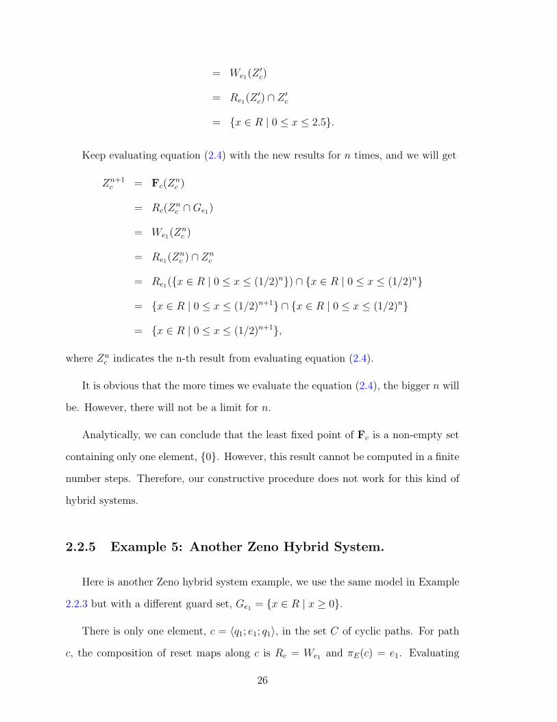
2.2.5 Example 5: Another Zeno Hybrid System.
Here is another Zeno hybrid system example, we use the same model in Example
2.2.3 but with a different guard set, Ge1 = {x ∈ R | x ≥ 0}.
There is only one element, c = 〈q1; e1; q1〉, in the set C of cyclic paths. For path
c, the composition of reset maps along c is Rc = We1 and πE(c) = e1. Evaluating
26

equation (2.4) with Zc as the guard Ge1 , we get
Z ′c = Fc(Rn
∞)
= Rc(Rn∞ ∩Ge1)
= We1(Ge1)
= Re1(Ge1) ∩Ge1
= {x ∈ R | x ≥ 1} ∩ {x ∈ R | x ≥ 0}
= {x ∈ R | x ≥ 1}.
Keep evaluating equation (2.4) with Z ′c, we get
Z ′′c = Fc(Z
′c)
= Rc(Z′c ∩Ge1)
= We1(Z′c)
= Re1(Z′c) ∩ Z ′
c
= {x ∈ R | x ≥ 2}.
Keep evaluating equation (2.4) with the new results for n times, we will get
Zn+1c = Fc(Z
nc )
= Rc(Znc ∩Ge1)
= We1(Znc )
= Re1(Znc ) ∩ Zn
c
= Re1({x ∈ R | x ≥ n}) ∩ {x ∈ R | x ≥ n}
= {x ∈ R | x ≥ n + 1} ∩ {x ∈ R | x ≥ n}
= {x ∈ R | x ≥ n + 1},
where Znc indicates the n-th result from evaluating equation (2.4).
27

It is obvious that the more times we evaluate the equation (2.4), the bigger n will
be. However, there will not be a limit for n.
Analytically, noting that R∞ contains ∞, we can conclude that the least fixed
point of Fc is a set containing only one element {∞}. Therefore this system may
have a Zeno behavior, we need to introduce a post-Zeno state for describing the
dynamics after the Zeno point. The completion process is omitted in this report.
However, we have to point out that this fixed point set cannot be computed in a
finite number steps. Therefore, our constructive procedure does not work for this
kind of hybrid systems.
28

Chapter 3
Approximate Simulation
In [11], we proposed an operational semantics for simulating hybrid system models.
The key idea of the operational semantics is to treat a complete simulation as a
sequence of unit executions, where a unit execution consists of two phases. The
discrete phase of execution handles all discrete events at the same time point, and
the continuous phase resolves the continuum between two consecutive discrete events.
When simulating a Zeno hybrid system model, we encounter more challenging
practical issues. The first difficulty is that before the Zeno time point, there will be
an infinite number of discrete transitions (events). Handling a discrete event takes
a non-zero time. So it is impossible to handle all discrete transitions in a finite
time interval. In other words, the simulation gets stuck near the Zeno time point.
The second difficulty is numerical errors, which make it impractical to get an exact
simulation. We will first elaborate on the second issue, and then we will come back
to the first issue in subsection 3.3.
29

3.1 Numerical Errors
There are two sources of numerical errors: round-off error and truncation error1.
Round-off error arises from using a finite number of bits in a computer to represent
a real value. We denote this kind of difference as η. Then we can say that each
integration operation will incur a round-off error of order η, denoted as O(η). Round-
off error accumulates. Suppose we integrate with a fixed step-size solver with a
integration step size as h. In order to simulate over a unit time interval, we need h−1
integration steps, then the total round-off error is O(η/h). Clearly, the bigger the
step size, the fewer integration steps, the smaller the total round-off error. Similar
results can be inferred for variable step-size solvers.
Truncation error comes from the integration algorithms used by practical ODE
solvers. For example, an nth-order explicit Runge-Kutta method, which is derived
to match the first n + 1 terms of Taylor’s expansion, has a local truncation error of
O(hn+1) and an accumulated truncation error of O(hn). Note that both truncation
errors decrease as h decreases. Ideally we will get no truncation errors as h → 0.
The total numerical error ε for an ODE solver using an nth-order explicit Runge-
Kutta method is the sum of the round-off error and truncation error,
ε ∼ η/h + hn. (3.1)
We can see that with a big integration step size h, the total error is dominated by
truncation error, whereas round-off error dominates with a small step size. Therefore,
although it is desirable to choose a small step size to reduce truncation error, the
accuracy of a calculation result may not be increased due to the accumulation of
round-off error. If we take the derivative of (3.1) with respect to h, then we get that
1We will not give a thorough discussion of numerical errors, which have been extensively studied,e.g. in [12]. We would rather briefly review and explain the important trade-offs when choosingintegration step sizes.
30

when h ∼ η1/(n+1) the total error ε reaches its minimum O(ηn/(n+1)) . Therefore, in
practice, we need to set a lower bound for both the integration step size and error
tolerance (or value resolution) of integration results. We denote them as h0 and ε0
respectively, where
h0 ∼ η1/(n+1), ε0 ∼ ηn/(n+1).
For a good simulation, accuracy is one concern and efficiency is another objective.
Efficiency for numerical integration is usually measured in terms of computation time
or the number of computing operations. Using a big integration step size is an effective
way to improve efficiency but with the penalty of loss of accuracy. So there is a trade-
off. Furthermore, step sizes have upper bounds that are enforced by the consistency,
convergence, and stability requirements when deploying practical integration methods
on concrete ODEs [12]. Therefore, most practical adaptive ODE solvers embed a
mechanism inside the integration process to adjust the step size to meet the desired
tolerance of integration results, so that efficiency gets improved while maintaining the
required accuracy at the same time.
In summary, a practical ODE solver usually specifies a minimum integration step
size h0, some small error tolerance ε0, and an algorithm to adapt step size to meet
requirements on both efficiency and accuracy.
3.2 Computation Difficulties
It is well-known that numerical integration in general can only deliver an approx-
imation to the exact solution of an initial value ODE. However, the distance of the
approximation from the exact solution is controllable for certain kinds of vector fields.
For example, if a vector field satisfies a Lipschitz condition along the time interval
where it is defined, we can constrain the integration results to reside within a neigh-
31
borhood of the exact solution by introducing more bits for representing values to get
better precision and integrating with a small step size.
The same difficulties that arise in numerical integration also appear in event detec-
tion. A few algorithms have been developed to solve this problem [13]–[15]. However,
there is still a fundamental unsolvable difficulty: we can only get the simulation time
close to the time point where an event occurs, but we are not assured of being able
to determine that point precisely.
Simulating a Zeno hybrid system poses another fundamental difficulty. We will
first explain it through a simple continuous-time example with dynamics
x(t) = 1/(t− 1), x(0) = 0, t ∈ [0, 2]. (3.2)
We can analytically find the solution for this example, x(t) = ln |t − 1|. However,
getting the same result through simulation is difficult. Suppose the simulation starts
with t = 0. As t approaches 1, the derivative x(t) keeps decreasing without bound. To
satisfy the convergence and stability requirements, the step size h has to be decreased.
When the step size becomes smaller than h0, round-off error is not neglectable any
more and the simulation results become unreliable. Trying to reduce the step size
further doesn’t help, because the disturbance from round-off error will dominate.
A similar problem arises when simulating Zeno hybrid system models. Recall that
Zeno executions have an infinite number of discrete events (transitions) before reach-
ing the Zeno time point, and the time intervals between two consecutive transitions
shrink to 0. When the time interval becomes less than h0, round-off errors again
dominate.
In summary, it is impractical to precisely simulate the behavior of a Zeno model.
Therefore, similar to numerical integration, we need to develop a computationally
feasible way to approximate the exact model behavior. The objective is to give a
32

close approximation under the limits enforced by numerical errors. We will do this in
the next subsection.
3.3 Approximating Zeno Behaviors
In Sect. 2, we have described how to specify the behaviors of a Zeno hybrid system
before and after the Zeno time point and how to develop transitions from pre-Zeno
states to post-Zeno states. The construction procedure works for guards which are
arbitrary sets. However, assuming that each guard is the sub-levelset of a function
(or collection of functions) simplifies the framework for studying transitions to post-
Zeno states. Therefore, we assume that a transition going from a pre-Zeno state to a
post-Zeno state has a guard expression of form,
Gec = {x ∈ Rn∞ | gec(x) ≤ 0}, (3.3)
for every c ∈ C, where ec = h−1(c) and gec : Rn∞ → Rk
∞. Furthermore, we assume
that gec(x) is continuously differentiable.
In this section, we will develop an algorithm such that the complete model behav-
ior can be simulated. As the previous subsection pointed out, we can only approximate
the model behaviors before the Zeno time point. Therefore, the first issue is to be
able to tell how close the simulation results are to the exact solutions before the Zeno
time point. This will decide when the transitions from pre-Zeno states to post-Zeno
states are taken. The second issue is how to establish the initial conditions of the
dynamics after the Zeno time point from the approximated simulation results.
33

3.3.1 Issue 1: Relaxing Guard Expressions.
To solve the first issue, we first relax the guard conditions defining the transitions
from the pre-Zeno states to the post-Zeno states; if the current states fall into a
neighborhood of the Zeno states (the states at the Zeno time point), the guard is
enabled and transition is taken. Note that when the transition is taken, the system
has a new dynamics and the rest of the events before the Zeno time point, which are
infinite in number, are discarded. Therefore the computation before the approximated
Zeno time point can be finished in finite time.
A practical problem now is to define a good neighborhood such that the approxi-
mation is “close enough” to the exact Zeno behavior. We propose two criteria. The
first criterion is based on the error tolerance ε02. We rewrite (3.3) as
Gε0ec
= {x ∈ Rn∞ | gec(x) ≤ ε0}, (3.4)
meaning if x(t) is the solution of x = fq(x) with q = s(ec), and if the evaluation
result of gec(x(t)) falls inside [0, ε0], the simulation results of x(t) will be thought as
close enough to the exact solution at the Zeno time point, and the transition will be
taken. In fact, because ε0 is the smallest amount that can be reliably distinguished,
any value in [0, ε0] will be treated the same.
The second criterion is based on the minimum step size h0. Suppose the evaluation
result of gec(x(t)) is outside of the range [0, ε0]. If it takes less than h0 time for the
dynamics to drive the value of gec(x(t)) down to 0, then we will treat the current states
as close enough to the Zeno states. This criterion prevents the numerical integration
from failing with a step size smaller than h0, which may be caused by some rapidly
changing dynamics, such as those in (3.2).
2If gec(x) is a vector valued function, then ε0 is a vector with ε0 as the elements.
34
We first get a linear approximation to function gec(x(t)) around t0 (cf. [13], [15]),
gec(x(t0 + h)) = gec(x(t0)) +∂gec(x)
∂x· fq(x) |x=x(t0) ·h + O(h2), (3.5)
where h is the integration step size. Because we are interested in the model’s behavior
when h is close to h0, where h is very small, we can discard the O(h2) term in (3.5).
We are interested in how long it takes for the value of function gec(x(t0)) to go to 0,
so we calculate the required step size by solving (3.5),
h = − gec(x(t0))∂gec (x)
∂x· fq(x) |x=x(t0)
. (3.6)
Now we say that if h < h0, the states are close enough to the Zeno point. So we
rewrite the boolean expression (3.3) as
Gh0ec
=
{x ∈ Rn
∞ | − gec(x)∂gec (x)
∂x· fq(x)
≤ h0
}. (3.7)
In the end, we give a complete approximated guard expression of the transition
ec from a pre-Zeno state to a post-Zeno state:
Gapproxec
= Gε0ec∪Gh0
ec.
This means that if either guard expression in (3.4) and (3.7) evaluates to be true, the
transition will be taken. Performing this process on each guard in the set {Gec | c ∈
C} we obtain the set {Gapproxec
| c ∈ C}. Note that to ensure deterministic transitions,
we also subtract the same set from the original guard sets defined in (2.6). Replacing
the guard expressions given in Sect. 2 with these approximated ones, we obtain an
approximation to the completed hybrid system H , Happrox
. This is the completed
hybrid system that is implemented for simulation.
3.3.2 Issue 2: Reinitialization.
The other issue is how to reinitialize the initial continuous states of the new
dynamics defined in a post-Zeno state. Theoretically, these initial continuous states
35

are just the states at the Zeno time point, meaning that they satisfy the guard
expression in (3.3). This is guaranteed by the identity reset maps associated with
the transitions.
In some circumstances, like the examples discussed in this report, the initial con-
tinuous states can be explicitly and precisely calculated. However, in general, if there
are more variables involved in guard expressions than the constraints enforced by
guard expressions, we cannot resolve all initial states. In this case, we have to use the
simulation results as part of the initial states. Clearly, since in simulation we do not
actually reach the Zeno time point, the initial states are just approximations. Con-
sequently, the simulation of the dynamics of post-Zeno states will be approximation
too.
36
Chapter 4
Conclusion
In this report, a systematic method is introduced for completing hybrid systems
through the introduction of new post-Zeno states and transitions to these states at
the Zeno point. A way to approximate model behaviors at Zeno points is developed
such that the simulation does not halt nor break down. With these solutions, a Zeno
hybrid system model can be simulated beyond its Zeno point and its dynamics is
revealed completely.
37

References
[1] J. Zhang, K. H. Johansson, J. Lygeros, and S. Sastry, “Zeno hybrid systems,” Int. J. Robust
and Nonlinear Control, vol. 11, no. 2, pp. 435–451, 2001.
[2] A. D. Ames, A. Abate, and S. Sastry, “Sufficient conditions for the existence of zeno behavior,”
in 44th IEEE Conference on Decision and Control and European Control Conference ECC,
2005.
[3] A. D. Ames, P. Tabuada, and S. Sastry, “On the stability of Zeno equilibria,” in Hybrid Systems:
Computation and Control (HSCC), J. P. Hespanha and A. Tiwari, Eds., vol. LNCS 3927. Santa
Barbara, CA, USA: Springer-Verlag, 2006, pp. 34 – 48.
[4] K. H. Johansson, J. Lygeros, S. Sastry, and M. Egerstedt, “Simulation of zeno hybrid au-
tomata,” in Proceedings of the 38th IEEE Conference on Decision and Control, Phoenix, AZ,
1999.
[5] A. D. Ames and S. Sastry, “Blowing up affine hybrid systems,” in 43rd IEEE Conference on
Decision and Control, 2004.
[6] P. J. Mosterman, “An overview of hybrid simulation phenomena and their support by simulation
packages,” in Hybrid Systems: Computation and Control (HSCC), F. Varager and J. H. v.
Schuppen, Eds., vol. LNCS 1569. Springer-Verlag, 1999, pp. 165–177.
[7] A. D. Ames, H. Zheng, R. Gregg, and S. Sastry, “Is there life after zeno? taking executions
past the breaking (zeno) point,” in American Control Conference (ACC), 2006.
[8] A. van der Schaft and H. Schumacher, An Introduction to Hybrid Dynamical Systems, ser.
Lecture Notes in Control and Information Sciences 251. Springer-Verlag, 2000.
[9] J. Lygeros, Lecture Notes on Hybrid Systems. ENSIETA 2-6/2/2004, 2004.
[10] B. A. Davey and H. A. Priestley, Introduction to Lattices and Order, 2nd ed. Cambridge
University Press, 2002.
[11] E. A. Lee and H. Zheng, “Operational semantics of hybrid systems,” in Hybrid Systems: Com-
putation and Control (HSCC), M. Morari and L. Thiele, Eds., vol. LNCS 3414. Zurich,
Switzerland: Springer-Verlag, 2005, pp. pp. 25–53.
[12] R. L. Burden and J. D. Faires, Numerical analysis, 7th ed. Brroks/Cole, 2001.
[13] L. F. Shampine, I. Gladwell, and R. W. Brankin, “Reliable solution of special event location
problems for odes,” ACM Trans. Math. Softw., vol. 17, no. 1, pp. 11–25, 1991.
38

[14] T. Park and P. I. Barton, “State event location in differential-algebraic models,” ACM Trans-
actions on Modeling and Computer Simulation (TOMACS), vol. 6, no. 2, pp. 137–165, 1996.
[15] J. M. Esposito, V. Kumar, and G. J. Pappas, “Accurate event detection for simulating hybrid
systems,” in Hybrid Systems: Computation and Control (HSCC), vol. LNCS 2034. London,
UK: Springer-Verlag, 2001, pp. 204–217.
39


![A Hybrid Approach for Simulating Human Motion in ...gamma.cs.unc.edu/DHM/casa10.pdfA Hybrid Approach for Simulating Human Motion in Constrained Environments Jia Pan], Liangjun Zhangy,](https://static.fdocuments.in/doc/165x107/5f18805bae452971a61a5f27/a-hybrid-approach-for-simulating-human-motion-in-gammacsuncedudhm-a-hybrid.jpg)