Simulated surface wave arrivals near Antipode

Get me out of here, faaaaaassstttt…..!!

Normal Modes & Earth’s Free OscillationsIn a nutshell: Normal modes

are simply another solution for the wave equation.

String Modes

€

∇2u =1

v 2

∂ 2u

∂t 2

Start with wave equation:

€

u(x, t) = Acos(ωt − kx)

Known solution so far:

€

u(x,t) = f (x± vt)(Generic) (Special)

Mode Solution to Wave Equation: A solution that separates out time and space dependence (note: the spatial locations of nodes are independent of time!).

Mode-wave duality----represent traveling wave as a weighted mode sum.

€

u(x, t) = AnUn (x,ωn )cos(ωn t)0

∞

∑

€

y(x, t) = AnUn (x,ωn )cos(ωn t)Let’s investigate this

=2L/nNow, the string example tells us that the length of string L = n half cycles

€

Un (x,ω) = sin(ωnx /v)Eigenfunction(i.e., a guess solution)

n=vk=2v/Dependencies of An: (1) source characteristics of vibration

(2) source time function

€

∂2y(x, t)

∂x 2= AnUn ' '(x,ωn )cos(ωn t)

Plug into Wave Eqn.

€

∂2y(x, t)

∂t 2= −Anωn

2Un (x,ωn )cos(ωn t)Wave Eqn.

€

AnUn ' '(x,ωn )cos(ωn t) = −An

ω2

v 2Un (x,ωn )cos(ωn t)

€

Un ' '(x,ωn ) = −ω2

v 2Un (x,ωn )

This is an Eigenvalue problem, i.e., A mathematical ‘machine’ acts on a function ends up a scalar multiply by the function.

€

−n

2

v 2sin(ωnx /v) = −

ωn2

v 2Un (x,ωn )

€

Un = sin(nπx /L)

1D string modesn = mode number (start with 1) = number of half cycles = number of peaks

n-1 = number of nodes (stationary points)

Figure taken from http://www.blazelabs.com/f-p-wave.asp

Standing Waves in 2-3 D

Left: Vertically shaking a cylinder of water with a constant frequency.

Below: Sand patterns on a “shake table”. Set vibration to a frequency and wait until sand patterns form. Like strings, this requires multiple tries to excite interesting-looking modes.. Mode summation = simulating movements by adding all the small patterns with variable weights.

Normal modes (standing waves) of the earth

€

u(r, θ, φ) = n Alm

m

∑l

∑n

∑ n fl(r) x lm (θ, φ)1 2 4 4 3 4 4 e inω l

mt

€

n Alm = weights of eigenfunctions, depends on source

n fl(r) = radial eigenfunction; shows variation with depth

xlm (θ, φ) = surface vector eigenfunction

€

nωlm = eigenfrequency, m is not needed for laterally

homogeneous earth

The earth “rings like a bell” after a big earthquake. This ringing will often last for days, even weeks. This process can be called an excitation of Earth’s normal modes, or free oscillations.

EarthquakeU

The surface eigenfunctions are related to spherical harmonics:

€

Ylm (θ,φ) = (−1)m

(2l +1)

4π

(l − m)!

(l + m)!

⎡

⎣ ⎢ ⎤

⎦ ⎥

1/ 2

Plm (cosθ)e imφ

where Plm is associated Legendre Polynomial

€

Plm (x) =

(1− x 2)m / 2

2l l!

d l+m

dx l+m(x 2 −1)l

and the azimuthal order, m, varies over

€

−l ≤ m ≤ l (degeneracy)

Ylm is complex

Angular order l givesnumber of nodal lines

m=0 ---> small circle about pole

l=m ---> goes through pole

1

2

1 2

3

1 2

3

4

Symmetric spherical harmonics

zonal sectoral tesseral

L = 12 example

€

sinθYl 'm '*(θ,φ)Yl

m (θ,φ)dθdφ = δ l ' lδm'm0

π

∫0

2π

∫

Spherical harmonics give a nice set of basis functions that are Orthogonal (linearly independent) that spans the spherical surface,Precisely the reason why it is so useful in earth sciences.

Orthogonal because

Two types of Normal Modes: (1) Toroidal Mode (SH waves) (2) Spheroidal Mode (P-SV motion)

Toroidal Modes:

€

x lm = Tl

m = 0, 1

sinθ

∂Ylm (θ,φ)

∂φ,

-∂Ylm (θ,φ)

∂θ

⎛

⎝ ⎜

⎞

⎠ ⎟

For u=(ur, u, u)

€

uT (r, θ, φ) = n Alm nfl(r) Tl

m (θ, φ)e inω lmt

m

∑l

∑n

∑Motions are purely SH, n = radial order

l = angular order m = azimuthal order0 T 2

This is where spherical harm is tied to modes

Examples of ToroidalModes:

Fundamental mode

n=0

Number of nodal

Lines = l-1

€

0T20

€

0T21

€

0T32

€

1T20€

0T30

€

0T1€

0T31

nTlm

Note: 1.there are differences in the number of nodal lines among spherical harm and modes 2.k, l and m have relations to depth, lat and lon (in a rotated system)

Spheroidal modes: normal modes that describe the P-SV motions in the earth.

€

uS (r, θ, φ) = n Alm

n U l(r) Rlm (θ, φ) +n Vl(r) Sl

m (θ, φ)[ ]einω l

mt m=−l to l

∑l

∑n

∑Where,

€

Rlm = Yl

m (θ,φ), 0,0( )

€

Slm = 0,

∂Ylm (θ,φ)

∂φ,

1

sinθ

∂Ylm (θ,φ)

∂θ

⎛

⎝ ⎜

⎞

⎠ ⎟

(radial motion)

(horizontal)

l=number of surface nodel lines, l=0 is radial mode.

€

0S0

€

1S0 €

0S20

These are simple modes in 3D. The fundamental mode has no zero-crossing in amplitude (note: looks a bit like sensitivity function of surface waves!). In fact, normal modes and surface wave modes are related.

Mode Ray Duality and

-l diagram (similar in to f-k diagram in 1D)

Right picture: Note that the deeper the phase goes, the higher the frequency and the smaller the L.

Top Left: Surface wave mode branch (note how broad fundamental mode is, precisely why it is most useful observationally)

Free oscillations

Mode Wave Duality (all observable surface wave modes)

€

x = 2π / | kx |= 2πa /(l +1/2)

cx =n ωl/ | kx |=n ωla /(l +1/2)

(a = earth radius)

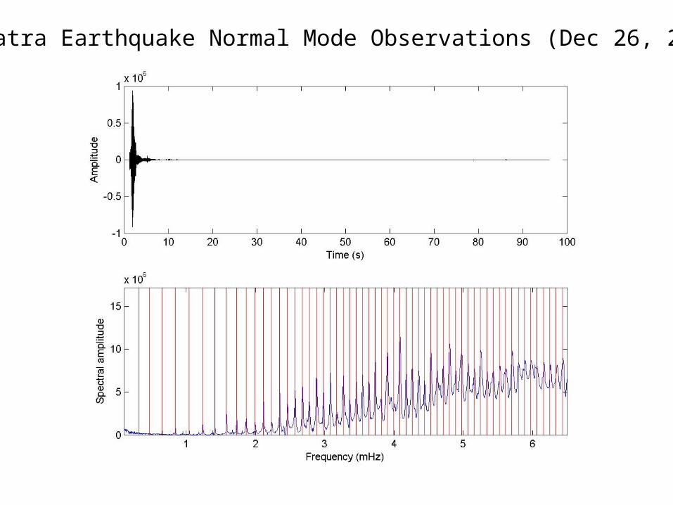
Sumatra Earthquake Normal Mode Observations (Dec 26, 2004)

Top: Mode observations by Fourier transforms of the time-domain recordings. Modes are usually very long periods and only comes in certain discrete frequencies.

Bottom plot: Mode Summations in the simulation of Love waves. This differs from a Reflectivity Method approach, but get the same results for simulating traveling waves. (Pro: Very fast if a mode catalogue exists, just pick and add.Con: Mode catalogue is HUGE for high-frequency simulations!

Mode Observations & Usage

Singlets and multiplets:Each azimuthal orderrepresents a spectral Peak. Without lateralvelocity and density variations, also withoutconsideration of earth’sellipticity, they all shouldcome at the same frequency. The fact they all have the Same frequency is called

“degeneracy” of mode. Each of them is called a “Singlet”. Their superposition forms one spectral peak called “multiplet”. But with those above factors present, They will split (called

“mode splitting”.

Earth’s Rotation Effect

Non-polarlatitude

Polarlatitude

Rotational effect: more significant at longer periods, high speeds, and islarger than effect of heterogeneity.

Effect of Heterogeneity

This is a densitymap obtained frommeasurements of normal mode splitting

Good thing aboutNormal modes:

Depends on the particleMotions with depth (radial eigenfunctions),Some modes have motionsas deep as the core. ThatGives us information aboutthe “Very Deep Earth”.

Shear and Bulk-sound speedsof the Core-Mantle-Boundary

€

δ = (δαKα + δβKβ + δρKρ )dVV

∫

€

v _bs =k

ρ

Rayleigh waves are solutions to the elastic wave equation given a half space and a free surface. Their amplitude decays exponentially with depth. The particle motion is elliptical (larger vertical than horizontal, retrograde near surface) and consists of motion in the plane through source and receiver.

SH-type surface waves do not exist in a half space. However in layered media, particularly if there is a low-velocity surface layer. Love waves exist which are dispersive, propagate along the surface. Their amplitude also decays exponentially with depth.

Free oscillations are standing waves which form after big earthquakes inside the Earth (useful ones are Mw 8-9.5, unfortunately). Spheroidal and toroidal eigenmodes correspond are analogous concepts to P and shear waves. Modes sum up to produce both body waves and surface waves (not the other way round).

Summary of Surface Wave and Modes