SIMPLE STRESSES AND STRAINS

Mechanics of Materials

Mechanics of materials deals with the elastic behavior of materials and the stability of members. Mechanics of

materials concepts are used to determine the stress and deformation of axially loaded members, connections,

torsional members, thin-walled pressure vessels, beams, eccentrically loaded members, and columns.

Simple Stresses & Strains

Stress is the internal resistance offered by the body per unit area. Stress is represented as force per unit area.

Typical units of stress are N/m2, ksi and MPa. There are two primary types of stresses: normal stress and shear

stress. Normal stress, , is calculated when the force is normal to the surface area; where as the shear stress, ,

is calculated when the force is parallel to the surface area.

A

P areatonormal __

A

P areatoparallel __

Linear strain (normal strain, longitudinal strain, axial strain), , is a change in length per unit length. Linear

strain has no units. Shear strain, , is an angular deformation resulting from shear stress. Shear strain may be

presented in units of radians, percent, or no units at all.

L

tan__

Height

areatoparallel [ in radians]

Hooke‘s law is a simple mathematical relationship between elastic stress and strain: stress is proportional to

strain. For normal stress, the constant of proportionality is the modulus of elasticity (Young’s Modulus), E.

E

Poisson’s ratio, , is a constant that relates the lateral strain to the axial strain for axially loaded members.

axial

lateral

Theoretically, Poisson’s ratio could vary from zero to 0.5, but typical values are 0.35 for aluminum and 0.3 for

steel and maximum value of 0.5 for rubber.

Hooke’s law may also be applied to a plane element in pure shear. For such an element, the shear stress is

linearly related to the shear strain, by the shear modulus (also known as the modulus of rigidity), G.

G

For an elastic isotropic material, the modulus of elasticity E, shear modulus G, and Poisson’s ratio are related

by

12

EG

12GE

The bulk modulus (K) describes volumetric elasticity, or the tendency of an object's volume to deform when

under pressure; it is defined as volumetric stress over volumetric strain, and is the inverse of compressibility.

The bulk modulus is an extension of Young's modulus to three dimensions.

For an elastic, isotropic material, the modulus of elasticity E, bulk modulus K, and Poisson’s ratio are related

by

21K3E

Uniaxial Loading and Deformation

The deformation, , of an axially loaded member of original length L can be derived from Hooke’s law.

Tension loading is considered to be positive; compressive loading is negative. The sign of the deformation will

be the same as the sign of the loading.

AE

PL

ELL

This expression for axial deformation assumes that the linear strain is proportional to the normal stress

E and that the cross-sectional area is constant.

When an axial member has distinct sections differing in cross-sectional area or composition, superposition is

used to calculate the total deformation as the sum of individual deformations.

AE

LP

AE

PL

When one of the variables (e.g., A), varies continuously along the length,

AE

dLP

AE

PdL

The new length of the member including the deformation is given by

LL f

The algebraic deformation must be observed.

Elastic Strain Energy In Uniaxial Loading

Strain energy, also known as internal energy per unit volume stored in a deformed material. The strain energy is

equivalent to the work done by the applied force. Simple work is calculated as the product of a force moving

through a distance.

Work = force x distance

= FdL

Work per volume =AL

FdL

= d

Work per unit volume corresponds to the area under the stress-strain curve.

For an axially loaded member below the proportionality limit, the total strain energy is given by,

AE

LPPU

22

1 2

The strain energy per unit volume is

EAL

Uu

2

2

Three Dimensional Strains

Hooke’s law, previously defined for axial loads and for pure shear, can be derived for three-dimensional

Stress-strain relationships and written in terms of the three elastic constants, E, G, and . The following

equations can be used to find the stresses and strains on the differential element in Fig. (1).

zyxxE

1

xzyyE

1

yxzzE

1

G

xy

xy

G

yz

yz

G

zxzx

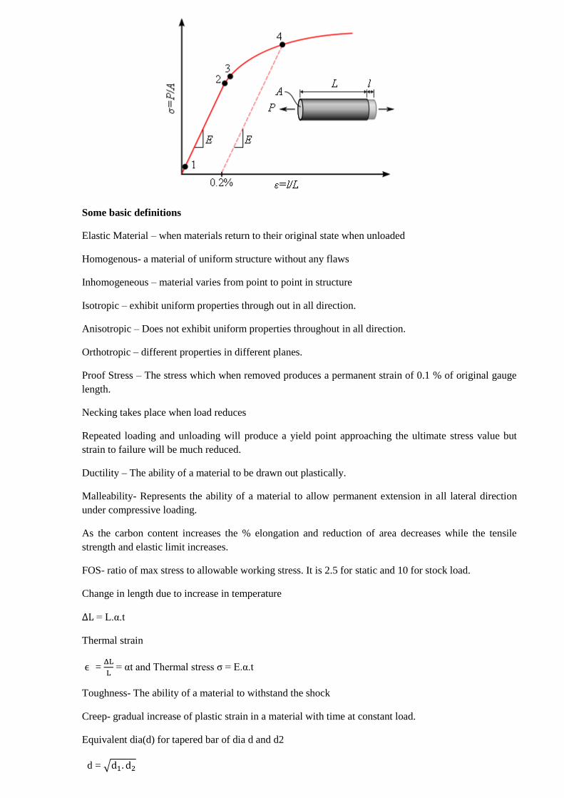
Stress-Strain curve

Some basic definitions

Elastic Material – when materials return to their original state when unloaded

Homogenous- a material of uniform structure without any flaws

Inhomogeneous – material varies from point to point in structure

Isotropic – exhibit uniform properties through out in all direction.

Anisotropic – Does not exhibit uniform properties throughout in all direction.

Orthotropic – different properties in different planes.

Proof Stress – The stress which when removed produces a permanent strain of 0.1 % of original gauge

length.

Necking takes place when load reduces

Repeated loading and unloading will produce a yield point approaching the ultimate stress value but

strain to failure will be much reduced.

Ductility – The ability of a material to be drawn out plastically.

Malleability- Represents the ability of a material to allow permanent extension in all lateral direction

under compressive loading.

As the carbon content increases the % elongation and reduction of area decreases while the tensile

strength and elastic limit increases.

FOS- ratio of max stress to allowable working stress. It is 2.5 for static and 10 for stock load.

Change in length due to increase in temperature

= L.α.t

Thermal strain

ϵ = = αt and Thermal stress σ = E.α.t

Toughness- The ability of a material to withstand the shock

Creep- gradual increase of plastic strain in a material with time at constant load.

Equivalent dia(d) for tapered bar of dia d and d2

d =

Compound Bars:

1. = . W

2. =

3. Common extension, x =

4. Difference in free length =

Thin-Walled Pressure Vessels: Cylindrical shells

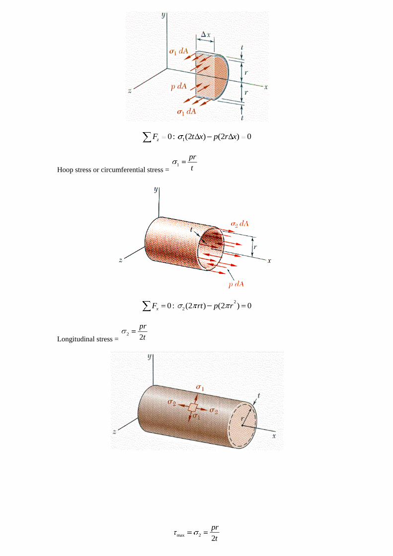
10: (2 ) (2 ) 0zF t x p r x

Hoop stress or circumferential stress = 1

pr

t

2

20: (2 ) (2 ) 0xF rt p r

Longitudinal stress = 2

2

pr

t

max 22

pr

t

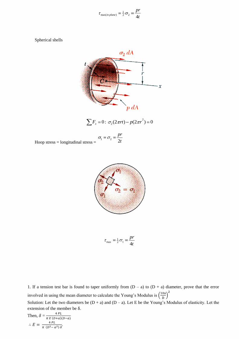
1max( ) 22

4in plane

pr

t

Spherical shells

2

20: (2 ) (2 ) 0xF rt p r

Hoop stress = longitudinal stress = 1 2

2

pr

t

1max 12

4

pr

t

1. If a tension test bar is found to taper uniformly from (D – a) to (D + a) diameter, prove that the error

involved in using the mean diameter to calculate the Young’s Modulus is

Solution: Let the two diameters be (D + a) and (D – a). Let E be the Young’s Modulus of elasticity. Let the

extension of the member be .

Then, =

.

If the mean diameter D is adopted, let be the computed Young’s modulus.

Then =

=

Hence, percentage error in computing Young’s modulus

=

= 100

= 100

= percent.

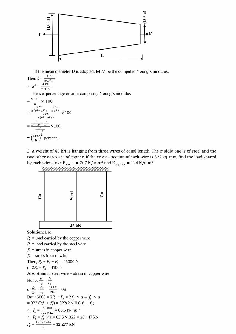
2. A weight of 45 kN is hanging from three wires of equal length. The middle one is of steel and the

two other wires are of copper. If the cross – section of each wire is 322 sq. mm, find the load shared

by each wire. Take = 207 N/ and = 124.N/ .

Solution: Let

= load carried by the copper wire

= load carried by the steel wire

= stress in copper wire

= stress in steel wire

Then, + + = 45000 N

or 2 + = 45000

Also strain in steel wire = strain in copper wire

Hence =

or = = = 06

But 45000 = 2 + = 2

= 322 (2 + ) = 322(2 0.6 + )

= = 63.5 N/

= a = 63.5 322 = 20.447 kN

= = 12.277 kN

45 kN

Ste

el

Cu

Cu

(D +

a)

(D +

a)

L

P P

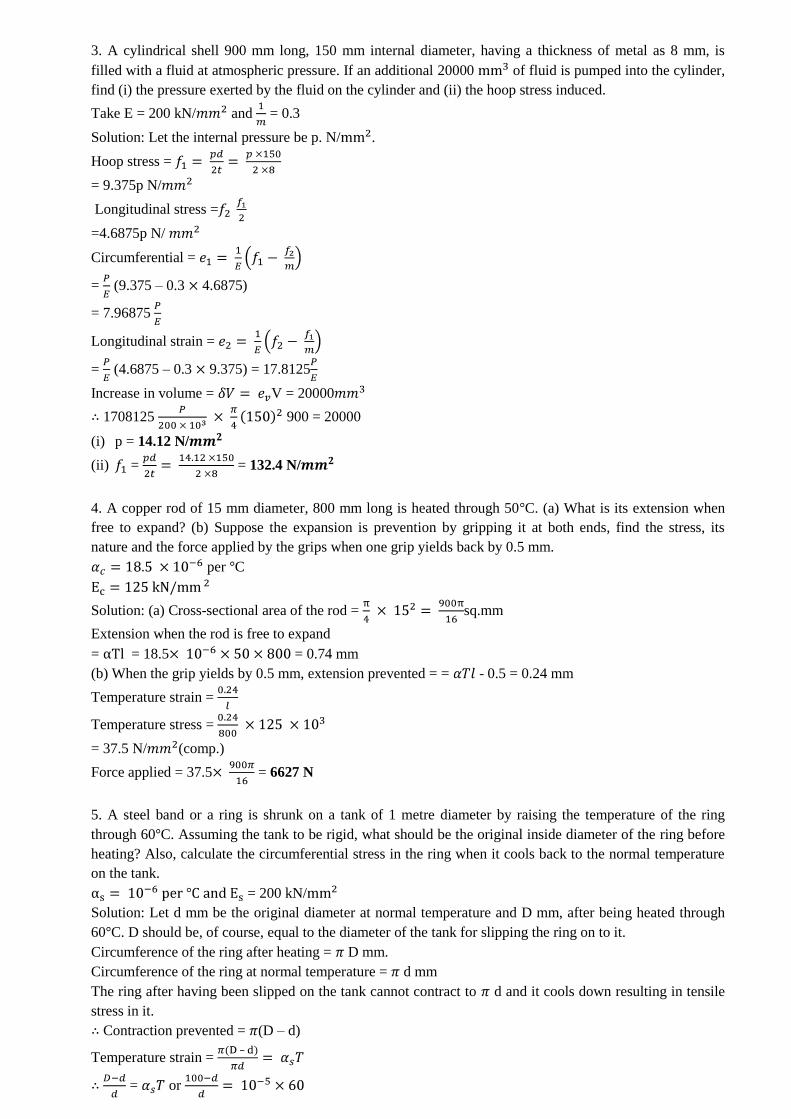
3. A cylindrical shell 900 mm long, 150 mm internal diameter, having a thickness of metal as 8 mm, is

filled with a fluid at atmospheric pressure. If an additional 20000 of fluid is pumped into the cylinder,

find (i) the pressure exerted by the fluid on the cylinder and (ii) the hoop stress induced.

Take E = 200 kN/ and = 0.3

Solution: Let the internal pressure be p. N/ .

Hoop stress =

= 9.375p N/

Longitudinal stress =

=4.6875p N/

Circumferential =

= (9.375 – 0.3 4.6875)

= 7.96875

Longitudinal strain =

= (4.6875 – 0.3 9.375) = 17.8125

Increase in volume = V = 20000

1708125 900 = 20000

(i) p = 14.12 N/

(ii) = = 132.4 N/

4. A copper rod of 15 mm diameter, 800 mm long is heated through 50 C. (a) What is its extension when

free to expand? (b) Suppose the expansion is prevention by gripping it at both ends, find the stress, its

nature and the force applied by the grips when one grip yields back by 0.5 mm.

per C

Solution: (a) Cross-sectional area of the rod = sq.mm

Extension when the rod is free to expand

= = 18.5 = 0.74 mm

(b) When the grip yields by 0.5 mm, extension prevented = = - 0.5 = 0.24 mm

Temperature strain =

Temperature stress =

= 37.5 N/ (comp.)

Force applied = 37.5 = 6627 N

5. A steel band or a ring is shrunk on a tank of 1 metre diameter by raising the temperature of the ring

through 60 C. Assuming the tank to be rigid, what should be the original inside diameter of the ring before

heating? Also, calculate the circumferential stress in the ring when it cools back to the normal temperature

on the tank.

= 200 kN/

Solution: Let d mm be the original diameter at normal temperature and D mm, after being heated through

60 C. D should be, of course, equal to the diameter of the tank for slipping the ring on to it.

Circumference of the ring after heating = D mm.

Circumference of the ring at normal temperature = d mm

The ring after having been slipped on the tank cannot contract to d and it cools down resulting in tensile

stress in it.

Contraction prevented = (D – d)

Temperature strain = –

= or

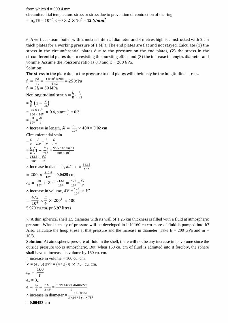
from which d = 999.4 mm

circumferential temperature stress or stress due to prevention of contraction of the ring

= TE = 60 = 12 N/

6. A vertical steam boiler with 2 metres internal diameter and 4 metres high is constructed with 2 cm

thick plates for a working pressure of 1 MPa. The end plates are flat and not stayed. Calculate (1) the

stress in the circumferential plates due to the pressure on the end plates, (2) the stress in the

circumferential plates due to resisting the bursting effect and (3) the increase in length, diameter and

volume. Assume the Poisson’s ratio as 0.3 and E = 200 GPa.

Solution:

The stress in the plate due to the pressure to end plates will obviously be the longitudinal stress.

= 25 MPa

= 2 = 50 MPa

Net longitudinal strain = -

=

= since = 0.3

= =

Increase in length, = 0.02 cm

Circumferential stain

= - = -

= =

= =

Increase in diameter, = d

= 0.0425 cm

=

Increase in volume, V =

5,970 cu.cm. pr 5.97 litres

7. A thin spherical shell 1.5 diameter with its wall of 1.25 cm thickness is filled with a fluid at atmospheric

pressure. What intensity of pressure will be developed in it if 160 cu.cm more of fluid is pumped into it?

Also, calculate the hoop stress at that pressure and the increase in diameter. Take E = 200 GPa and m =

10/3.

Solution: At atmospheric pressure of fluid in the shell, there will not be any increase in its volume since the

outside pressure too is atmospheric. But, when 160 cu. cm of fluid is admitted into it forcibly, the sphere

shall have to increase its volume by 160 cu. cm.

increase in volume = 160 cu. cm.

V = (4 / 3) = (4 / 3) cu. cm.

=

=

increase in diameter =

= 0.00453 cm

8. A compound tube is made by shrinking a thin steel tube on a thin brass tube. and brass tubes, and

and are the corresponding values of the Young’s Modulus. Show that for any tensile load, the extension

of the compound tube is equal to that of a single tube of the same length and total cross-sectional area but

having a Young’s Modulus of .

Solution:

= = strain …… (i)

Where and are stresses in steel and brass tubes respectively.

+ = P ……. (ii)

where P – total load on the compound tube.

From equations (i) and (ii); . + = P

= P

……. (iii)

Extension of the compound tube = dl = extension of steel or brass tube

= …….. (iv)

From equations (iii) and (iv);

= …….. (v)

Let E be the Young’s modulus of a tube of area ( + ) carrying the same load and undergoing the same

extension

= ……. (vi)

equation (v) = (vi)

= or E =

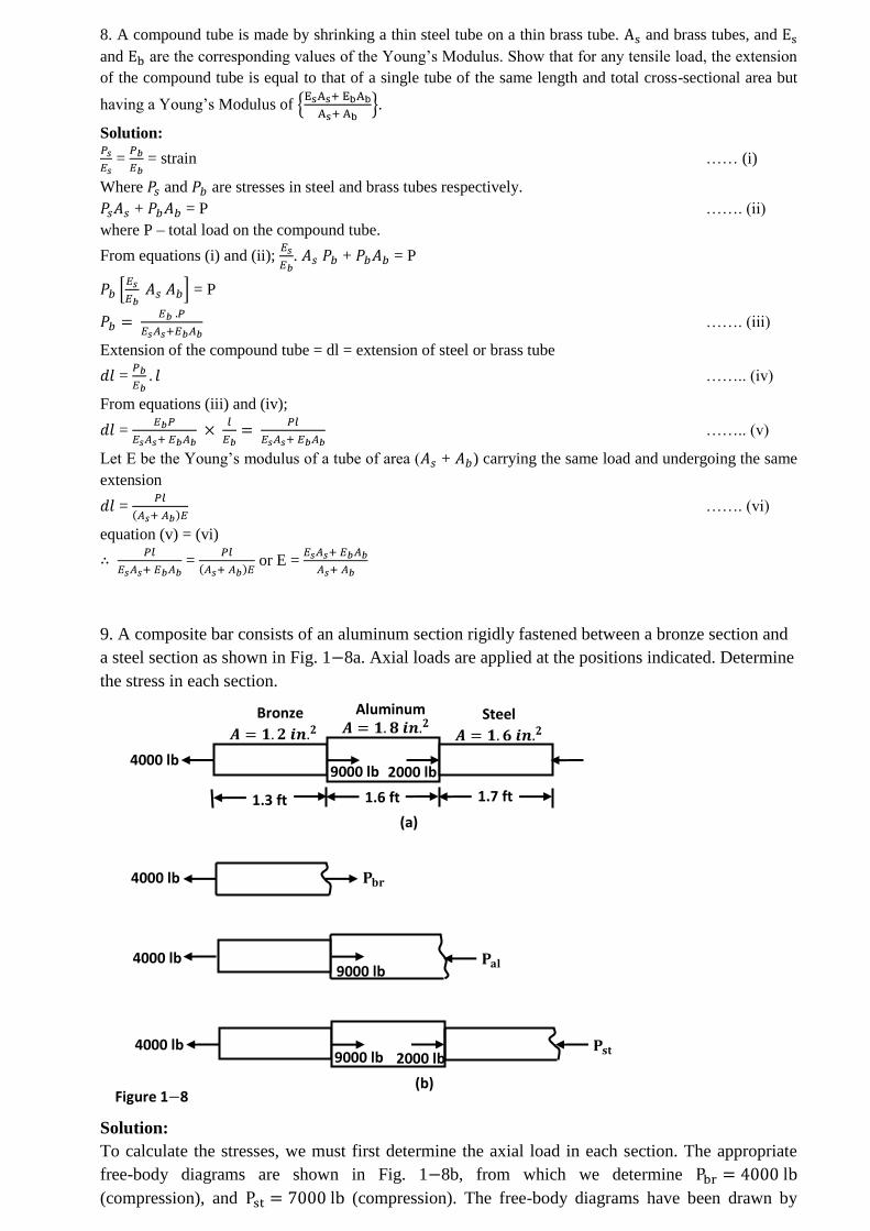
9. A composite bar consists of an aluminum section rigidly fastened between a bronze section and

a steel section as shown in Fig. 1 8a. Axial loads are applied at the positions indicated. Determine

the stress in each section.

Solution:

To calculate the stresses, we must first determine the axial load in each section. The appropriate

free-body diagrams are shown in Fig. 1 8b, from which we determine

(compression), and (compression). The free-body diagrams have been drawn by

Bronze

Aluminum

Steel

9000 lb 2000 lb

1.3 ft 1.6 ft 1.7 ft

(a)

4000 lb

4000 lb

4000 lb

4000 lb

(b) Figure 1 8

9000 lb

2000 lb 9000 lb

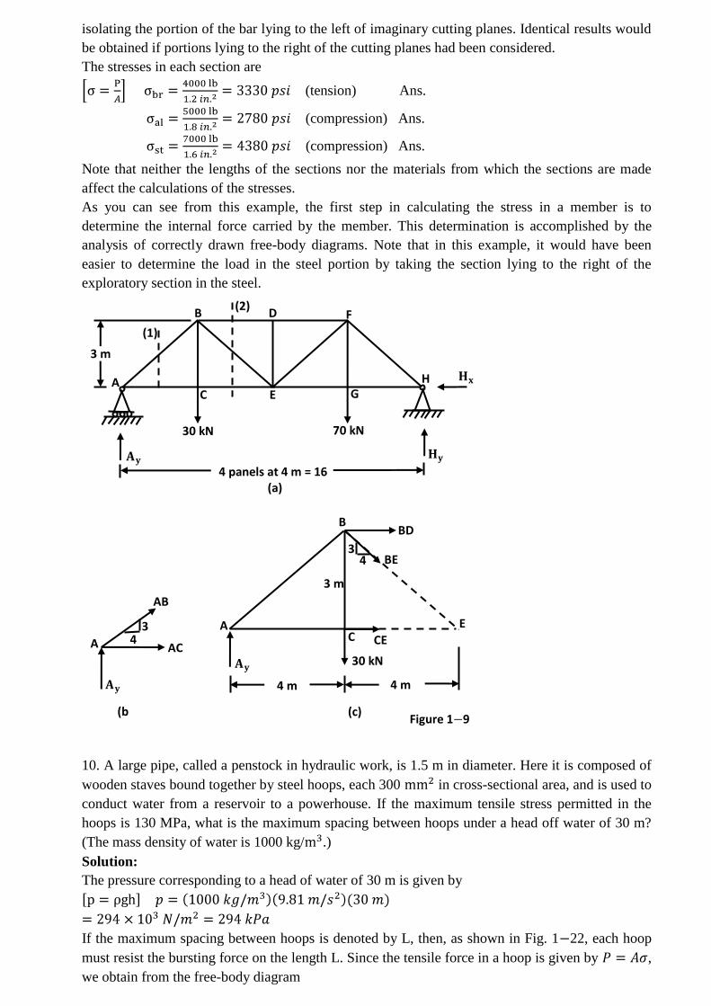
isolating the portion of the bar lying to the left of imaginary cutting planes. Identical results would

be obtained if portions lying to the right of the cutting planes had been considered.

The stresses in each section are

(tension) Ans.

(compression) Ans.

(compression) Ans.

Note that neither the lengths of the sections nor the materials from which the sections are made

affect the calculations of the stresses.

As you can see from this example, the first step in calculating the stress in a member is to

determine the internal force carried by the member. This determination is accomplished by the

analysis of correctly drawn free-body diagrams. Note that in this example, it would have been

easier to determine the load in the steel portion by taking the section lying to the right of the

exploratory section in the steel.

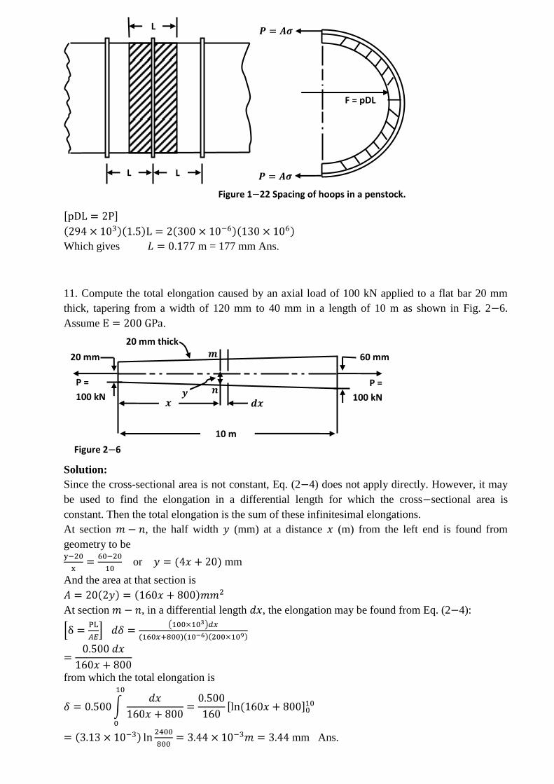
10. A large pipe, called a penstock in hydraulic work, is 1.5 m in diameter. Here it is composed of

wooden staves bound together by steel hoops, each 300 in cross-sectional area, and is used to

conduct water from a reservoir to a powerhouse. If the maximum tensile stress permitted in the

hoops is 130 MPa, what is the maximum spacing between hoops under a head off water of 30 m?

(The mass density of water is 1000 kg/ .)

Solution:

The pressure corresponding to a head of water of 30 m is given by

If the maximum spacing between hoops is denoted by L, then, as shown in Fig. 1 22, each hoop

must resist the bursting force on the length L. Since the tensile force in a hoop is given by ,

we obtain from the free-body diagram

A

AB

AC 4

3

(b

)

A

B BD

BE 3

4

3 m

C CE

E

30 kN

4 m 4 m

(c) Figure 1 9

4 panels at 4 m = 16

m (a)

30 kN 70 kN

3 m

(1)

A

B

C

(2) D

E

F

G H

Which gives m = 177 mm Ans.

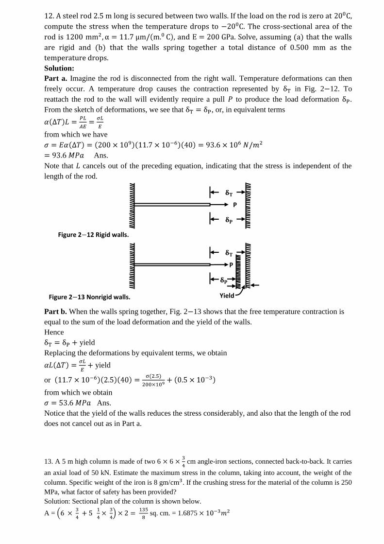
11. Compute the total elongation caused by an axial load of 100 kN applied to a flat bar 20 mm

thick, tapering from a width of 120 mm to 40 mm in a length of 10 m as shown in Fig. 2 6.

Assume .

Solution:

Since the cross-sectional area is not constant, Eq. (2 4) does not apply directly. However, it may

be used to find the elongation in a differential length for which the cross sectional area is

constant. Then the total elongation is the sum of these infinitesimal elongations.

At section , the half width (mm) at a distance (m) from the left end is found from

geometry to be

or mm

And the area at that section is

At section , in a differential length , the elongation may be found from Eq. (2 4):

from which the total elongation is

mm Ans.

20 mm thick

20 mm

P =

100 kN

10 m

60 mm

P =

100 kN

Figure 2 6

L

L L

F = pDL

Figure 1 22 Spacing of hoops in a penstock.

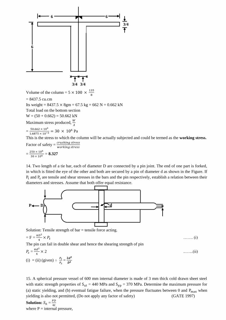
12. A steel rod 2.5 m long is secured between two walls. If the load on the rod is zero at C,

compute the stress when the temperature drops to . The cross-sectional area of the

rod is 1200 and . Solve, assuming (a) that the walls

are rigid and (b) that the walls spring together a total distance of 0.500 mm as the

temperature drops.

Solution:

Part a. Imagine the rod is disconnected from the right wall. Temperature deformations can then

freely occur. A temperature drop causes the contraction represented by in Fig. 2 12. To

reattach the rod to the wall will evidently require a pull to produce the load deformation .

From the sketch of deformations, we see that , or, in equivalent terms

from which we have

Ans.

Note that cancels out of the preceding equation, indicating that the stress is independent of the

length of the rod.

Part b. When the walls spring together, Fig. 2 13 shows that the free temperature contraction is

equal to the sum of the load deformation and the yield of the walls.

Hence

yield

Replacing the deformations by equivalent terms, we obtain

yield

or

from which we obtain

Ans.

Notice that the yield of the walls reduces the stress considerably, and also that the length of the rod

does not cancel out as in Part a.

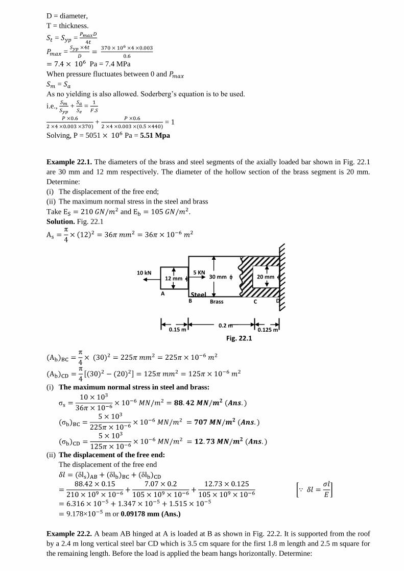
13. A 5 m high column is made of two 6 6 cm angle-iron sections, connected back-to-back. It carries

an axial load of 50 kN. Estimate the maximum stress in the column, taking into account, the weight of the

column. Specific weight of the iron is 8 gm/ . If the crushing stress for the material of the column is 250

MPa, what factor of safety has been provided?

Solution: Sectional plan of the column is shown below.

A = sq. cm. = 1.6875

P

P

Yield

Figure 2 12 Rigid walls.

Figure 2 13 Nonrigid walls.

Volume of the column = 5

= 8437.5 cu.cm

Its weight = 8437.5 8gm = 67.5 kg = 662 N = 0.662 kN

Total load on the bottom section

W = (50 + 0.662) = 50.662 kN

Maximum stress produced,

= Pa

This is the stress to which the column will be actually subjected and could be termed as the working stress.

Factor of safety =

= = 8.327

14. Two length of a tie bar, each of diameter D are connected by a pin joint. The end of one part is forked,

in which is fitted the eye of the other and both are secured by a pin of diameter d as shown in the Figure. If

and are tensile and shear stresses in the bars and the pin respectively, establish a relation between their

diameters and stresses. Assume that both offer equal resistance.

Solution: Tensile strength of bar = tensile force acting.

= F = ……. (i)

The pin can fail in double shear and hence the shearing strength of pin

= 2 ..…...(ii)

(i) = (ii) (given) =

15. A spherical pressure vessel of 600 mm internal diameter is made of 3 mm thick cold drawn sheet steel

with static strength properties of = 440 MPa and = 370 MPa. Determine the maximum pressure for

(a) static yielding, and (b) eventual fatigue failure, when the pressure fluctuates between 0 and when

yielding is also not permitted, (Do not apply any factor of safety) (GATE 1997)

Solution: =

where P = internal pressure,

D P d

6

6 6

3/4

3/4 3/4

D = diameter,

T = thickness.

= =

=

Pa = 7.4 MPa

When pressure fluctuates between 0 and

=

As no yielding is also allowed. Soderberg’s equation is to be used.

i.e., + =

+ = 1

Solving, P = 5051 Pa = 5.51 Mpa

Example 22.1. The diameters of the brass and steel segments of the axially loaded bar shown in Fig. 22.1

are 30 mm and 12 mm respectively. The diameter of the hollow section of the brass segment is 20 mm.

Determine:

(i) The displacement of the free end;

(ii) The maximum normal stress in the steel and brass

Take and .

Solution. Fig. 22.1

(i) The maximum normal stress in steel and brass:

(ii) The displacement of the free end:

The displacement of the free end

178× m or 0.09178 mm (Ans.)

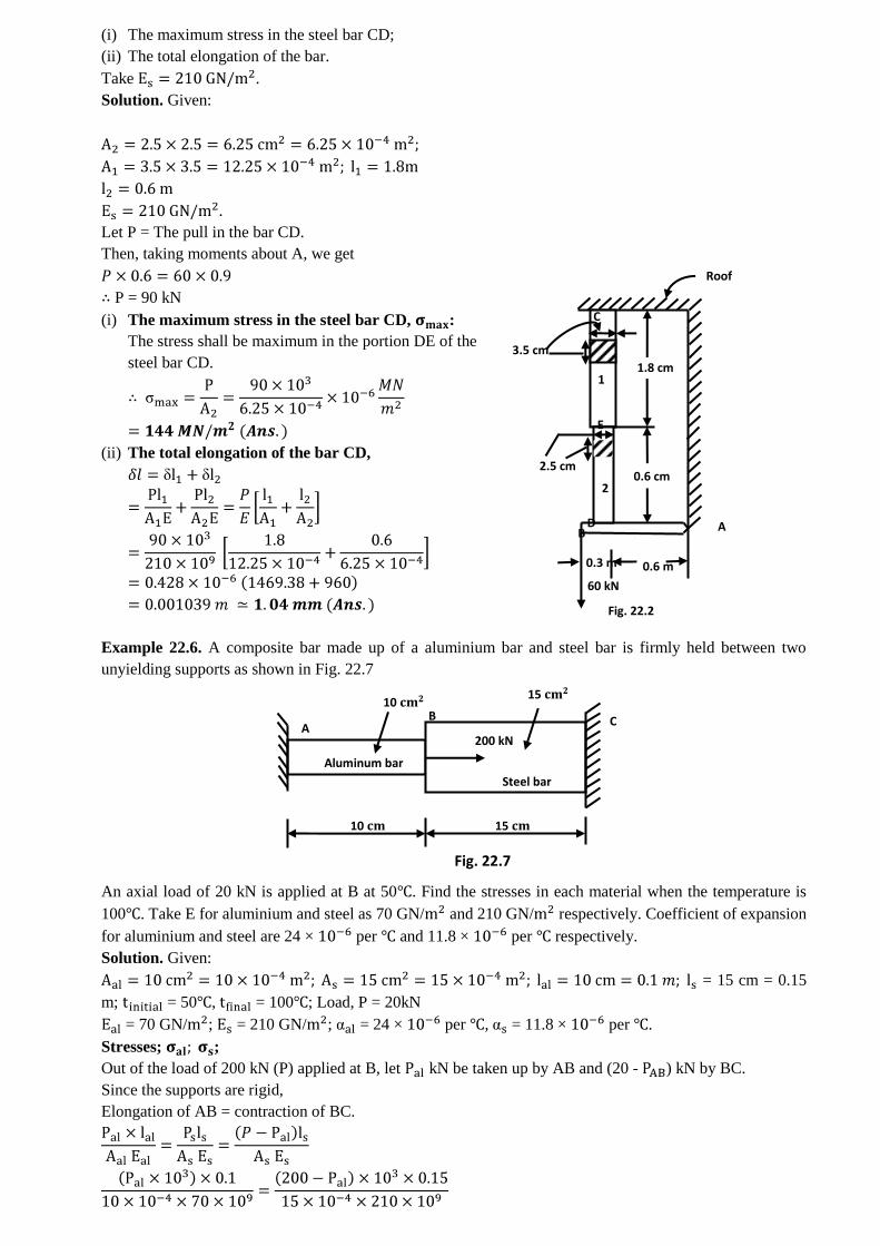
Example 22.2. A beam AB hinged at A is loaded at B as shown in Fig. 22.2. It is supported from the roof

by a 2.4 m long vertical steel bar CD which is 3.5 cm square for the first 1.8 m length and 2.5 m square for

the remaining length. Before the load is applied the beam hangs horizontally. Determine:

0.125 m

10 kN 12 mm

5 KN 30 mm 20 mm

A B Brass C D

0.15 m 0.2 m

Fig. 22.1

Steel

3.5 cm

Roof

C

A

2

1.8 cm

0.6 cm 2.5 cm

1

E

0.3 m

D B

60 kN

0.6 m

Fig. 22.2

(i) The maximum stress in the steel bar CD;

(ii) The total elongation of the bar.

Take .

Solution. Given:

Let P = The pull in the bar CD.

Then, taking moments about A, we get

∴ P = 90 kN

(i) The maximum stress in the steel bar CD, :

The stress shall be maximum in the portion DE of the

steel bar CD.

(ii) The total elongation of the bar CD,

Example 22.6. A composite bar made up of a aluminium bar and steel bar is firmly held between two

unyielding supports as shown in Fig. 22.7

An axial load of 20 kN is applied at B at 50℃. Find the stresses in each material when the temperature is

100℃. Take E for aluminium and steel as 70 GN/ and 210 GN/ respectively. Coefficient of expansion

for aluminium and steel are 24 × per ℃ and 11.8 × per ℃ respectively.

Solution. Given:

= 15 cm = 0.15

m; = 50℃, = 100℃; Load, P = 20kN

= 70 GN/ ; = 210 GN/ ; = 24 × per ℃, = 11.8 × per ℃.

Stresses; ;

Out of the load of 200 kN (P) applied at B, let kN be taken up by AB and (20 - ) kN by BC.

Since the supports are rigid,

Elongation of AB = contraction of BC.

10 15

15 10

B A

C

Aluminum bar

200 kN

Steel bar

Fig. 22.7

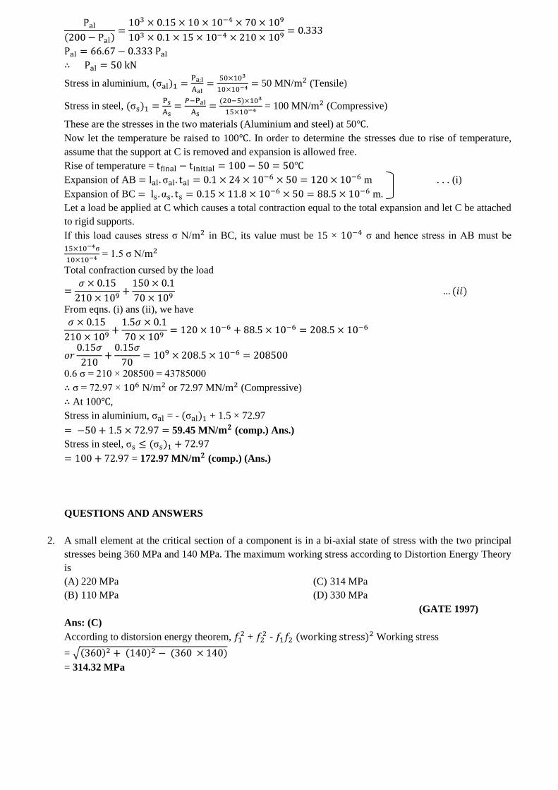
Stress in aluminium, 50 MN/ (Tensile)

Stress in steel, = 100 MN/ (Compressive)

These are the stresses in the two materials (Aluminium and steel) at 50℃.

Now let the temperature be raised to 100℃. In order to determine the stresses due to rise of temperature,

assume that the support at C is removed and expansion is allowed free.

Rise of temperature =

Expansion of AB m . . . (i)

Expansion of BC m.

Let a load be applied at C which causes a total contraction equal to the total expansion and let C be attached

to rigid supports.

If this load causes stress σ N/ in BC, its value must be 15 × σ and hence stress in AB must be

= 1.5 σ N/

Total confraction cursed by the load

From eqns. (i) ans (ii), we have

0.6 σ = 210 × 208500 = 43785000

∴ σ = 72.97 × N/ or 72.97 MN/ (Compressive)

∴ At 100℃,

Stress in aluminium, = - + 1.5 × 72.97

59.45 MN/ (comp.) Ans.)

Stress in steel,

= 172.97 MN/ (comp.) (Ans.)

QUESTIONS AND ANSWERS

2. A small element at the critical section of a component is in a bi-axial state of stress with the two principal

stresses being 360 MPa and 140 MPa. The maximum working stress according to Distortion Energy Theory

is

(A) 220 MPa

(B) 110 MPa

(C) 314 MPa

(D) 330 MPa

(GATE 1997)

Ans: (C)

According to distorsion energy theorem, + - Working stress

=

= 314.32 MPa

SHEARING FORCE AND BENDING MOMENT

Sign Conventions

The shear force, V at a section of a beam is the sum of all vertical forces acting on the beam between that

section and any one of its ends. It has units of Newtons, pounds, kips, etc. Shear force is not the same as shear

stress, since the area of the object is not considered.

The direction (i.e., to the left or right of the section) in which the summation proceeds is not important. Since

the values of shear will differ only in sign for summation to the left and right ends, the direction that results in

the fewest calculations should be selected.

endonetotion

iFV

__sec

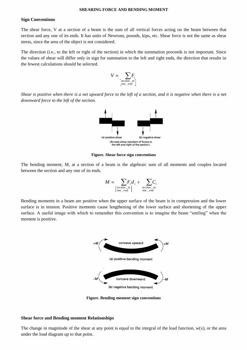
Shear is positive when there is a net upward force to the left of a section, and it is negative when there is a net

downward force to the left of the section.

Figure. Shear force sign conventions

The bending moment, M, at a section of a beam is the algebraic sum of all moments and couples located

between the section and any one of its ends.

endonetotion

i

endonetotion

ii CdFM

__sec

__sec

Bending moments in a beam are positive when the upper surface of the beam is in compression and the lower

surface is in tension. Positive moments cause lengthening of the lower surface and shortening of the upper

surface. A useful image with which to remember this convention is to imagine the beam “smiling” when the

moment is positive.

Figure. Bending moment sign conventions

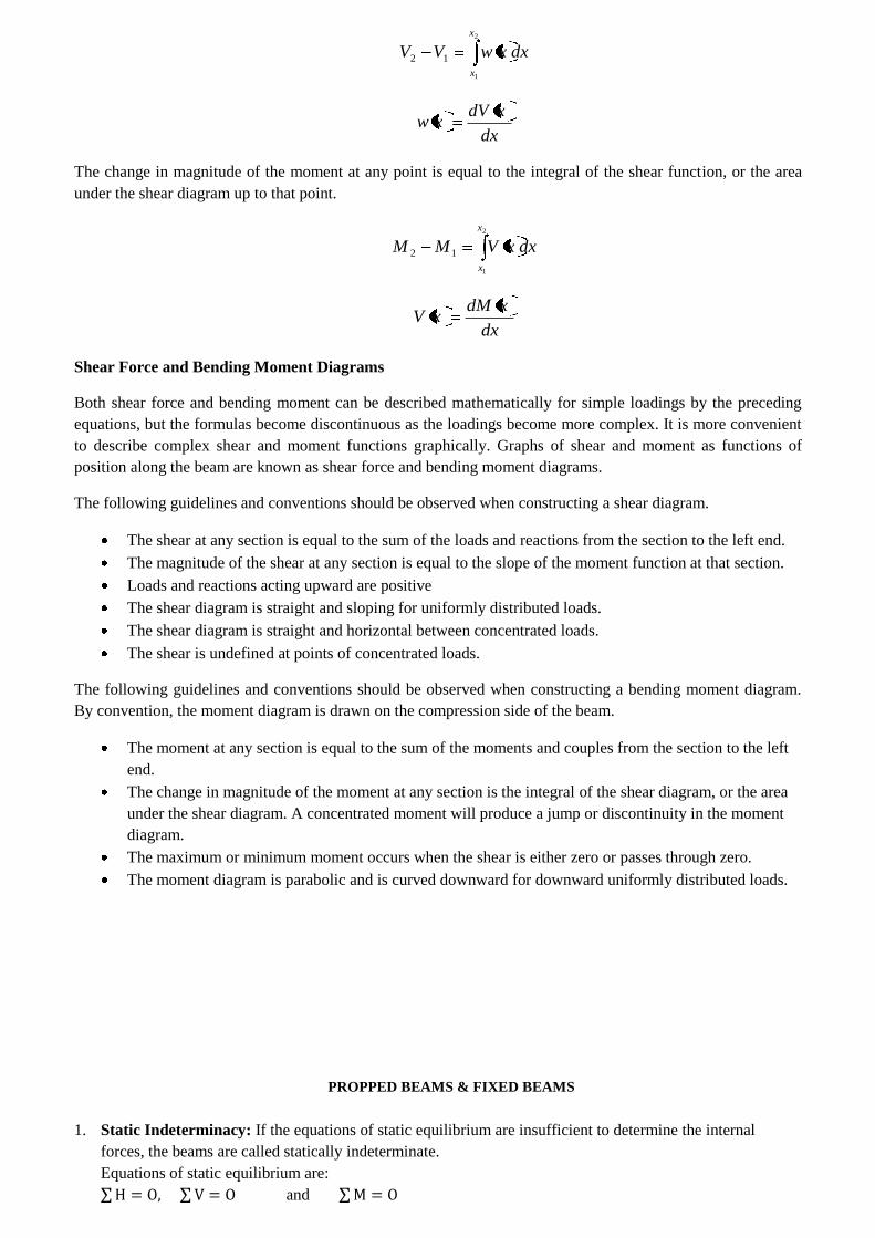
Shear force and Bending moment Relationships

The change in magnitude of the shear at any point is equal to the integral of the load function, w(x), or the area

under the load diagram up to that point.

dxxwVV

x

x

2

1

12

dx

xdVxw

The change in magnitude of the moment at any point is equal to the integral of the shear function, or the area

under the shear diagram up to that point.

dxxVMM

x

x

2

1

12

dx

xdMxV

Shear Force and Bending Moment Diagrams

Both shear force and bending moment can be described mathematically for simple loadings by the preceding

equations, but the formulas become discontinuous as the loadings become more complex. It is more convenient

to describe complex shear and moment functions graphically. Graphs of shear and moment as functions of

position along the beam are known as shear force and bending moment diagrams.

The following guidelines and conventions should be observed when constructing a shear diagram.

The shear at any section is equal to the sum of the loads and reactions from the section to the left end.

The magnitude of the shear at any section is equal to the slope of the moment function at that section.

Loads and reactions acting upward are positive

The shear diagram is straight and sloping for uniformly distributed loads.

The shear diagram is straight and horizontal between concentrated loads.

The shear is undefined at points of concentrated loads.

The following guidelines and conventions should be observed when constructing a bending moment diagram.

By convention, the moment diagram is drawn on the compression side of the beam.

The moment at any section is equal to the sum of the moments and couples from the section to the left

end.

The change in magnitude of the moment at any section is the integral of the shear diagram, or the area

under the shear diagram. A concentrated moment will produce a jump or discontinuity in the moment

diagram.

The maximum or minimum moment occurs when the shear is either zero or passes through zero.

The moment diagram is parabolic and is curved downward for downward uniformly distributed loads.

PROPPED BEAMS & FIXED BEAMS

1. Static Indeterminacy: If the equations of static equilibrium are insufficient to determine the internal

forces, the beams are called statically indeterminate.

Equations of static equilibrium are:

and

w/m

L/2 L/2 C A B

NOTE: shall be considered only if inclined horizontal loads exist.

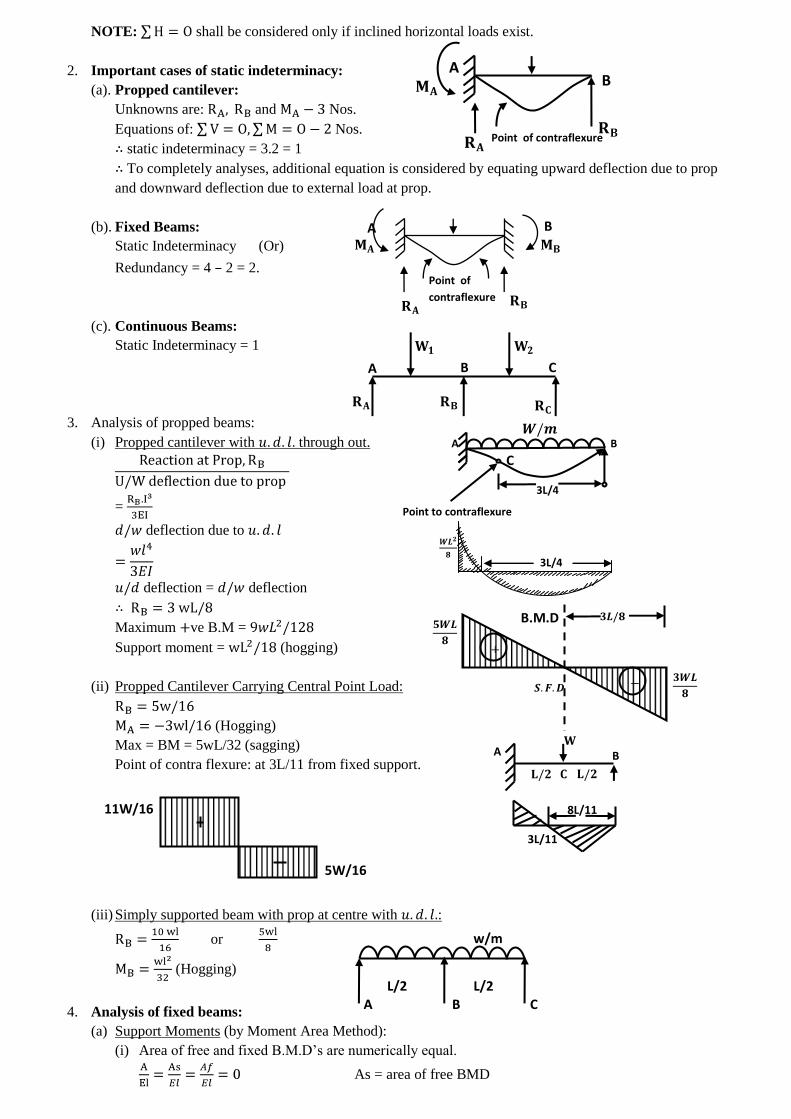
2. Important cases of static indeterminacy:

(a). Propped cantilever:

Unknowns are: and Nos.

Equations of: Nos.

∴ static indeterminacy = 3.2 = 1

∴ To completely analyses, additional equation is considered by equating upward deflection due to prop

and downward deflection due to external load at prop.

(b). Fixed Beams:

Static Indeterminacy (Or)

Redundancy = 4 – 2 = 2.

(c). Continuous Beams:

Static Indeterminacy = 1

3. Analysis of propped beams:

(i) Propped cantilever with through out.

=

deflection due to

deflection = deflection

Maximum ve B.M =

Support moment = (hogging)

(ii) Propped Cantilever Carrying Central Point Load:

(Hogging)

Max = BM = 5wL/32 (sagging)

Point of contra flexure: at 3L/11 from fixed support.

(iii) Simply supported beam with prop at centre with :

or

(Hogging)

4. Analysis of fixed beams:

(a) Support Moments (by Moment Area Method):

(i) Area of free and fixed B.M.D‟s are numerically equal.

As = area of free BMD

5W/16

11W/16

A

B

Point of contraflexure

A

B

Point of

contraflexure

A B C

B

3L/4

Point to contraflexure

A

3L/4

C

A

B

3L/11

8L/11

B.M.D

W/2

W/2

S.F.D

B.M.D

0.212 L

S.F.D

a b

B.M.D

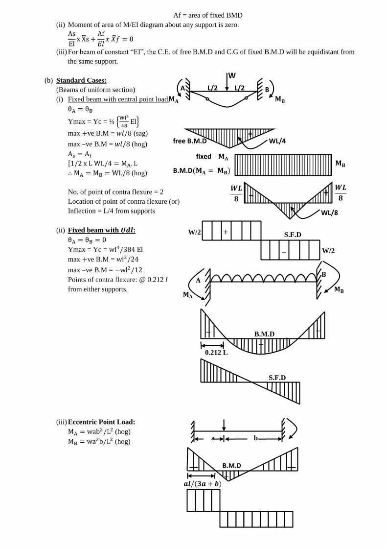
Af = area of fixed BMD

(ii) Moment of area of M/EI diagram about any support is zero.

(iii) For beam of constant “EI”, the C.E. of free B.M.D and C.G of fixed B.M.D will be equidistant from

the same support.

(b) Standard Cases:

(Beams of uniform section)

(i) Fixed beam with central point load.

Ymax = Yc = ¼

max ve B.M = (sag)

max –ve B.M = (hog)

∴ (hog)

No. of point of contra flexure = 2

Location of point of contra flexure (or)

Inflection = L/4 from supports

(ii) Fixed beam with :

Ymax = Yc =

max ve B.M =

max –ve B.M =

Points of contra flexure: @ 0.212

from either supports.

(iii) Eccentric Point Load:

(hog)

(hog)

WL/4 free B.M.D

fixed

B.M.D

WL/8

L/2 L/2

A B

W

al/(3a +

b)

L

a

L

(sagging)

(hogging)

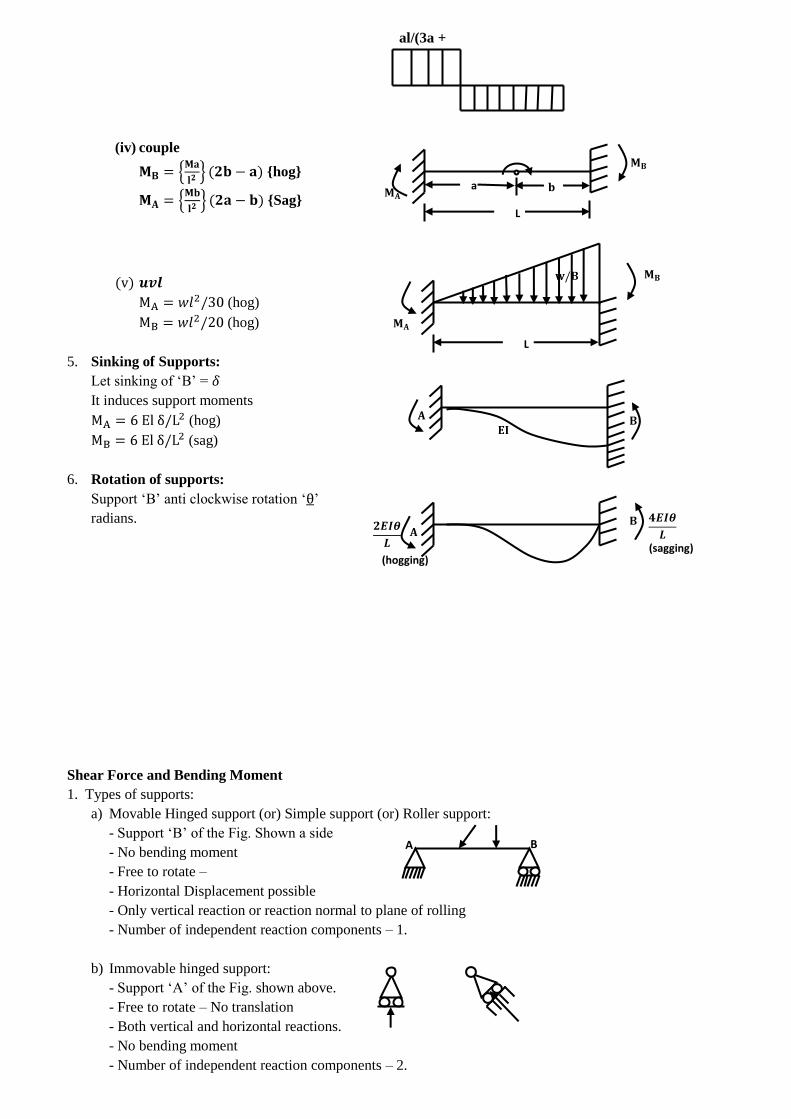
(iv) couple

{hog}

{Sag}

(v)

(hog)

(hog)

5. Sinking of Supports:

Let sinking of „B‟ =

It induces support moments

(hog)

(sag)

6. Rotation of supports:

Support „B‟ anti clockwise rotation „θ‟

radians.

Shear Force and Bending Moment

1. Types of supports:

a) Movable Hinged support (or) Simple support (or) Roller support:

- Support „B‟ of the Fig. Shown a side

- No bending moment

- Free to rotate –

- Horizontal Displacement possible

- Only vertical reaction or reaction normal to plane of rolling

- Number of independent reaction components – 1.

b) Immovable hinged support:

- Support „A‟ of the Fig. shown above.

- Free to rotate – No translation

- Both vertical and horizontal reactions.

- No bending moment

- Number of independent reaction components – 2.

B A

B A

2t

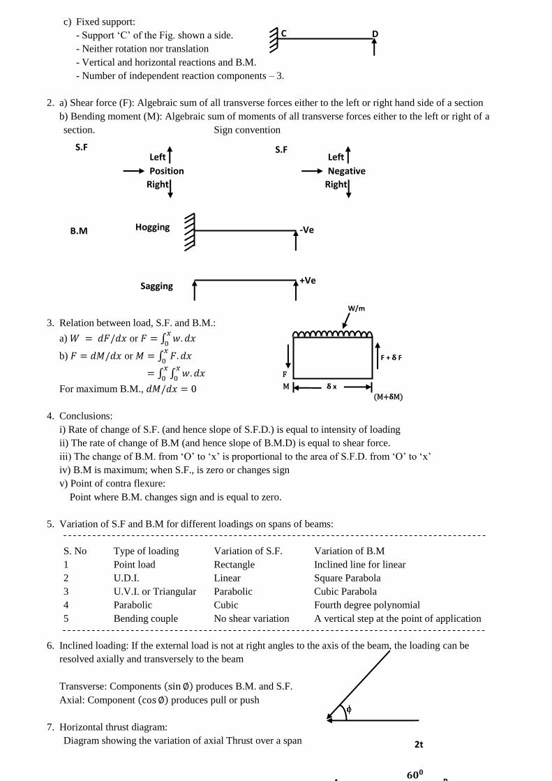
c) Fixed support:

- Support „C‟ of the Fig. shown a side.

- Neither rotation nor translation

- Vertical and horizontal reactions and B.M.

- Number of independent reaction components – 3.

2. a) Shear force (F): Algebraic sum of all transverse forces either to the left or right hand side of a section

b) Bending moment (M): Algebraic sum of moments of all transverse forces either to the left or right of a

section. Sign convention

3. Relation between load, S.F. and B.M.:

a) or

b) or

For maximum B.M.,

4. Conclusions:

i) Rate of change of S.F. (and hence slope of S.F.D.) is equal to intensity of loading

ii) The rate of change of B.M (and hence slope of B.M.D) is equal to shear force.

iii) The change of B.M. from „O‟ to „x‟ is proportional to the area of S.F.D. from „O‟ to „x‟

iv) B.M is maximum; when S.F., is zero or changes sign

v) Point of contra flexure:

Point where B.M. changes sign and is equal to zero.

5. Variation of S.F and B.M for different loadings on spans of beams:

S. No Type of loading Variation of S.F. Variation of B.M

1 Point load Rectangle Inclined line for linear

2 U.D.I. Linear Square Parabola

3 U.V.I. or Triangular Parabolic Cubic Parabola

4 Parabolic Cubic Fourth degree polynomial

5 Bending couple No shear variation A vertical step at the point of application

6. Inclined loading: If the external load is not at right angles to the axis of the beam, the loading can be

resolved axially and transversely to the beam

Transverse: Components produces B.M. and S.F.

Axial: Component produces pull or push

7. Horizontal thrust diagram:

Diagram showing the variation of axial Thrust over a span

S.F

Position

Left

Right

S.F

Negative

Left

Right

B.M -Ve

+Ve

Hogging

Sagging

D C

W/m

M

F + F

x

F

(M+ M)

H.T.D

8. Internal hinge: Bending moment is zero

9. Link: Only vertical force: Can not resist horizontal force „H‟ and B.M.

Point of contra flexures: The point or the points on the beam where the bending moment (B.M) changes

sign is defined as the point of contra flexure or point of inflexion.

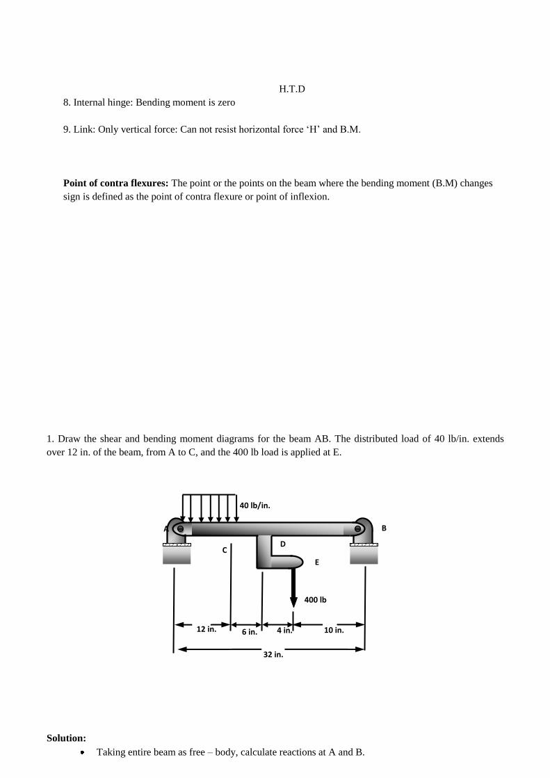
1. Draw the shear and bending moment diagrams for the beam AB. The distributed load of 40 lb/in. extends

over 12 in. of the beam, from A to C, and the 400 lb load is applied at E.

Solution:

Taking entire beam as free – body, calculate reactions at A and B.

B A

C D

E

400 lb

32 in.

10 in. 4 in. 6 in. 12 in.

40 lb/in.

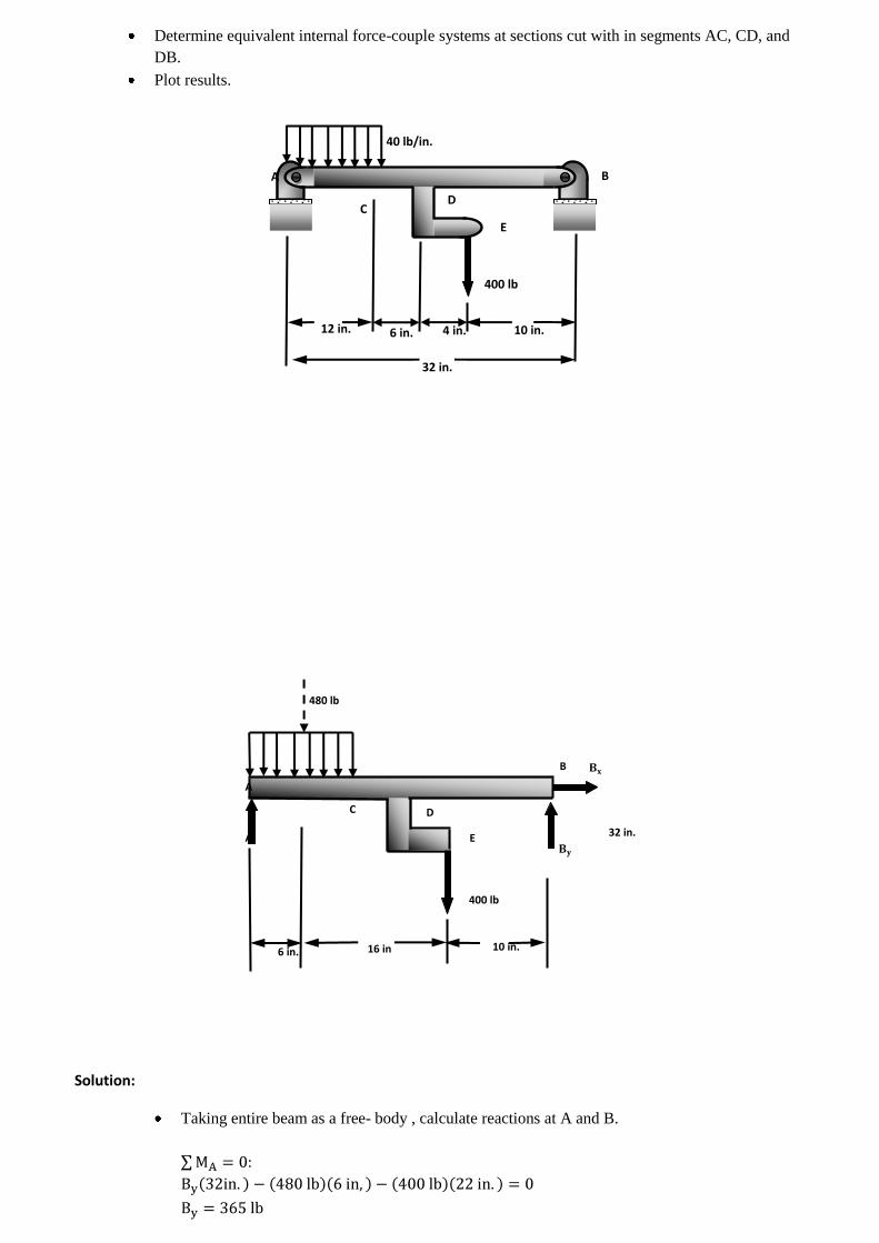
Determine equivalent internal force-couple systems at sections cut with in segments AC, CD, and

DB.

Plot results.

Solution:

Taking entire beam as a free- body , calculate reactions at A and B.

C D

E

400 lb

32 in.

10 in. 6 in.

16 in

B

A

480 lb

A

B A

C D

E

400 lb

32 in.

10 in. 4 in. 6 in. 12 in.

40 lb/in.

A = 515 lb

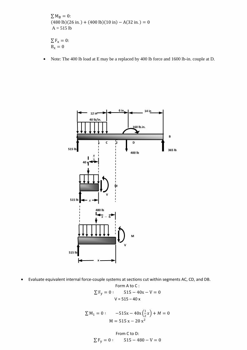
Note: The 400 lb load at E may be a replaced by 400 lb force and 1600 lb-in. couple at D.

Evaluate equivalent internal force-couple systems at sections cut within segments AC, CD, and DB.

Form A to C :

V = 515 – 40 x

From C to D:

365 lb

C D

400 lb

6 in.

40 lb/in.

14 in

B A

515 lb

12 in

160 lb.in.

2

1

40 x

515 lb

515 lb

480 lb

V

x

M

V

M

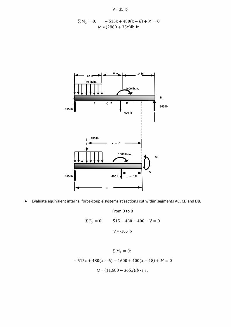
V = 35 lb

M =

Evaluate equivalent internal force-couple systems at sections cut within segments AC, CD and DB.

From D to B

V = -365 lb

M =

C D

400 lb

6 in.

40 lb/in.

14 in

B A

515 lb

12 in

1600 lb.in.

2 1 365 lb

3

1600 lb.in.

V

M

515 lb 400 lb

480 lb

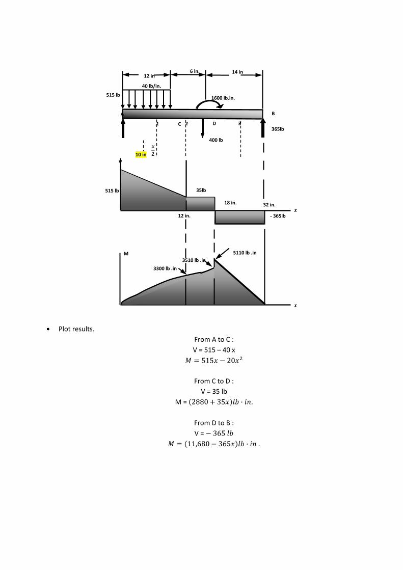
Plot results.

From A to C :

V = 515 – 40 x

From C to D :

V = 35 lb

M =

From D to B :

V =

C D

400 lb

6 in.

40 lb/in.

14 in

B A

515 lb

12 in

1600 lb.in.

2 1 3

10 in

V

- 365lb

35lb

32 in. 18 in.

365lb

3300 lb .in

5110 lb .in

3510 lb .in

12 in.

M

515 lb

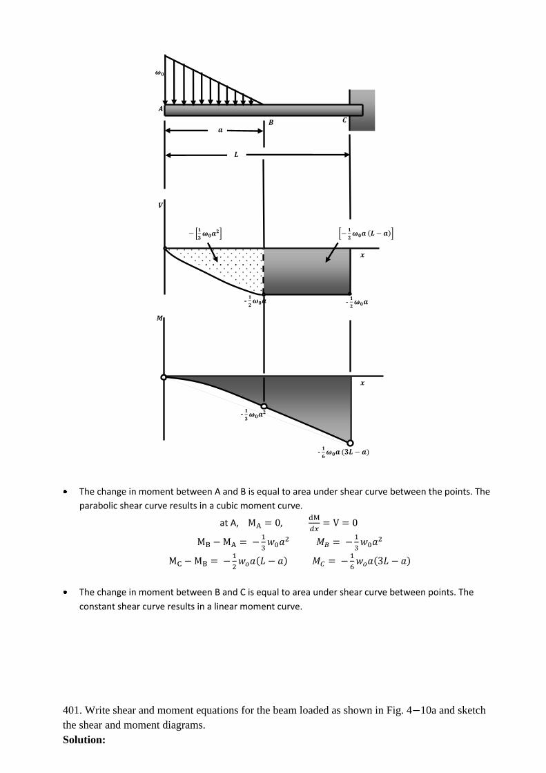
The change in moment between A and B is equal to area under shear curve between the points. The

parabolic shear curve results in a cubic moment curve.

at A,

The change in moment between B and C is equal to area under shear curve between points. The

constant shear curve results in a linear moment curve.

401. Write shear and moment equations for the beam loaded as shown in Fig. 4 10a and sketch

the shear and moment diagrams.

Solution:

-

-

- -

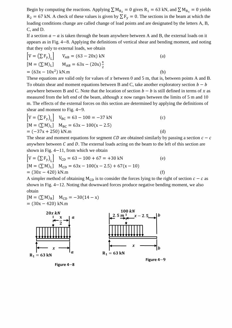
Begin by computing the reactions. Applying gives kN, and yields

kN. A check of these values is given by . The sections in the beam at which the

loading conditions change are called change of load points and are designated by the letters A, B,

C, and D.

If a section is taken through the beam anywhere between A and B, the external loads on it

appears as in Fig. 4 8. Applying the definitions of vertical shear and bending moment, and noting

that they only to external loads, we obtain

kN (a)

kN.m (b)

These equations are valid only for values of between 0 and 5 m, that is, between points A and B.

To obtain shear and moment equations between B and C, take another exploratory section

anywhere between B and C. Note that the location of section is still defined in terms of as

measured from the left end of the beam, although now ranges between the limits of 5 m and 10

m. The effects of the external forces on this section are determined by applying the definitions of

shear and moment to Fig. 4 9.

kN (c)

kN.m (d)

The shear and moment equations for segment are obtained similarly by passing a section

anywhere between and . The external loads acting on the beam to the left of this section are

shown in Fig. 4 11, from which we obtain

kN (e)

kN.m (f)

A simpler method of obtaining is to consider the forces lying to the right of section as

shown in Fig. 4 12. Noting that downward forces produce negative bending moment, we also

obtain

kN.m

Figure 4 8

Figure 4

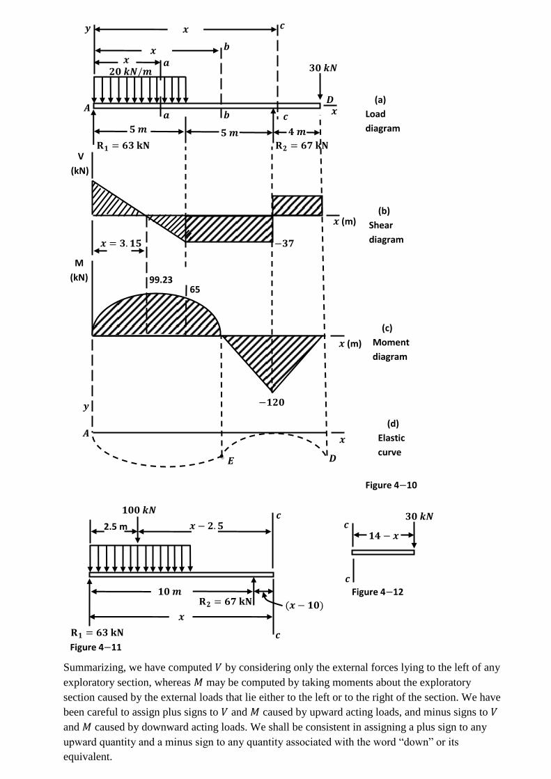
Summarizing, we have computed by considering only the external forces lying to the left of any

exploratory section, whereas may be computed by taking moments about the exploratory

section caused by the external loads that lie either to the left or to the right of the section. We have

been careful to assign plus signs to and caused by upward acting loads, and minus signs to

and caused by downward acting loads. We shall be consistent in assigning a plus sign to any

upward quantity and a minus sign to any quantity associated with the word “down” or its

equivalent.

2.5 m

Figure 4 11

Figure 4 12

(a)

Load

diagram

(m)

(m)

(b)

Shear

diagram

(c)

Moment

diagram

(d)

Elastic

curve

Figure 4 10

V

(kN)

M

(kN)

65 99.23

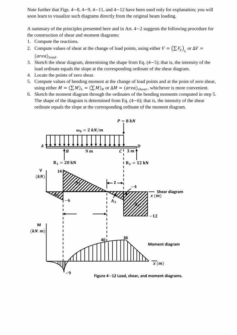
Note further that Figs. 4 8, 4 9, 4 11, and 4 12 have been used only for explanation; you will

soon learn to visualize such diagrams directly from the original beam loading.

A summary of the principles presented here and in Art. 4 2 suggests the following procedure for

the construction of shear and moment diagrams:

1. Compute the reactions.

2. Compute values of shear at the change of load points, using either or

.

3. Sketch the shear diagram, determining the shape from Eq. (4 5); that is, the intensity of the

load ordinate equals the slope at the corresponding ordinate of the shear diagram.

4. Locate the points of zero shear.

5. Compute values of bending moment at the change of load points and at the point of zero shear,

using either or , whichever is more convenient.

6. Sketch the moment diagram through the ordinates of the bending moments computed in step 5.

The shape of the diagram is determined from Eq. (4 6); that is, the intensity of the shear

ordinate equals the slope at the corresponding ordinate of the moment diagram.

Shear diagram

40 36

Moment diagram

Figure 4 12 Load, shear, and moment diagrams.

M

V

14

2

200 kN m

C A B

100 kN

2 m

200 kNm

2 m

100 kN

(b) S.F. Diagram

100 kN 100 kN

(c)B.M. Diagram

(a) Loaded beam

Fig. 22.15

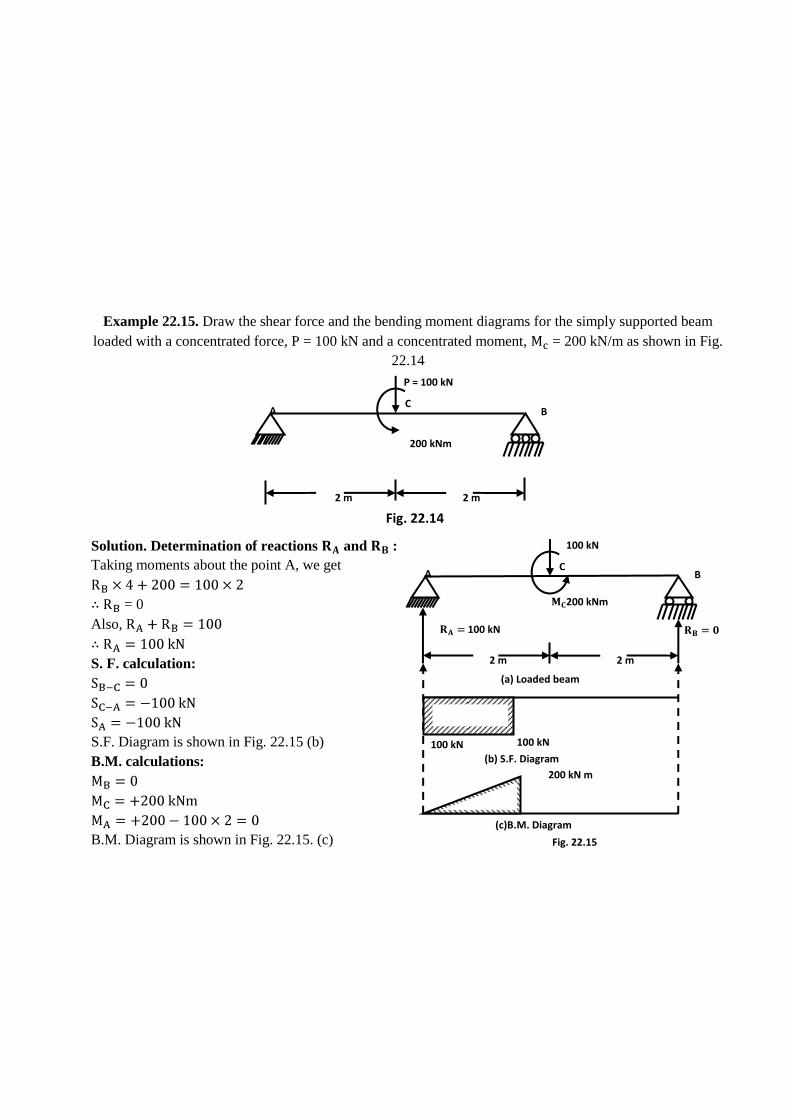
Example 22.15. Draw the shear force and the bending moment diagrams for the simply supported beam

loaded with a concentrated force, P = 100 kN and a concentrated moment, = 200 kN/m as shown in Fig.

22.14

Solution. Determination of reactions and :

Taking moments about the point A, we get

∴ = 0

Also,

∴

S. F. calculation:

S.F. Diagram is shown in Fig. 22.15 (b)

B.M. calculations:

B.M. Diagram is shown in Fig. 22.15. (c)

C A B

P = 100 kN

2 m

200 kNm

2 m

Fig. 22.14

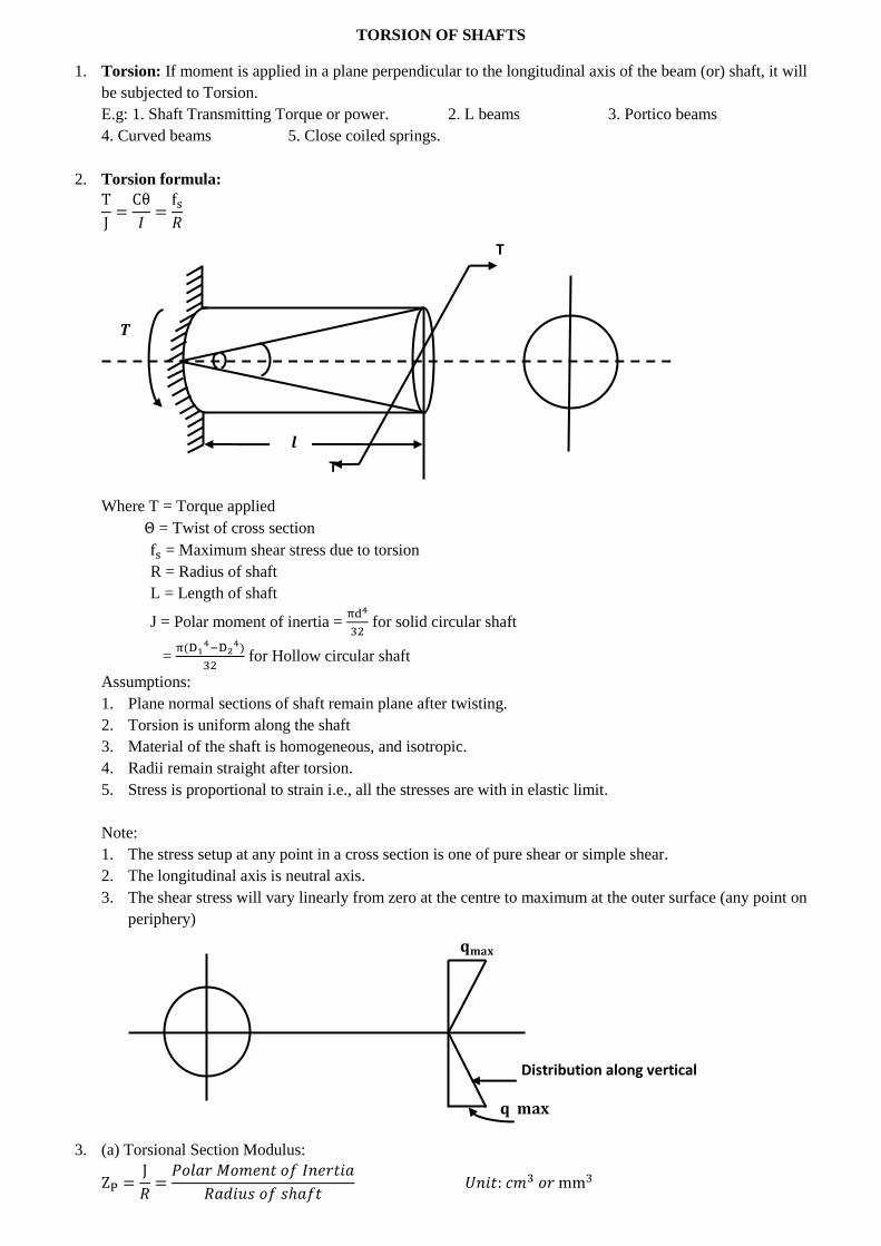
TORSION OF SHAFTS

1. Torsion: If moment is applied in a plane perpendicular to the longitudinal axis of the beam (or) shaft, it will

be subjected to Torsion.

E.g: 1. Shaft Transmitting Torque or power. 2. L beams 3. Portico beams

4. Curved beams 5. Close coiled springs.

2. Torsion formula:

Where T = Torque applied

Θ = Twist of cross section

= Maximum shear stress due to torsion

R = Radius of shaft

L = Length of shaft

J = Polar moment of inertia = for solid circular shaft

= for Hollow circular shaft

Assumptions:

1. Plane normal sections of shaft remain plane after twisting.

2. Torsion is uniform along the shaft

3. Material of the shaft is homogeneous, and isotropic.

4. Radii remain straight after torsion.

5. Stress is proportional to strain i.e., all the stresses are with in elastic limit.

Note:

1. The stress setup at any point in a cross section is one of pure shear or simple shear.

2. The longitudinal axis is neutral axis.

3. The shear stress will vary linearly from zero at the centre to maximum at the outer surface (any point on

periphery)

3. (a) Torsional Section Modulus:

Distribution along vertical

T

T

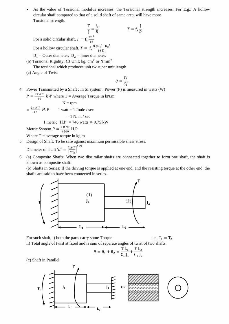
As the value of Torsional modulus increases, the Torsional strength increases. For E.g.: A hollow

circular shaft compared to that of a solid shaft of same area, will have more

Torsional strength.

For a solid circular shaft,

For a hollow circular shaft,

= Outer diameter, = inner diameter.

(b) Torsional Rigidity: CJ Unit: kg. or

The torsional which produces unit twist per unit length.

(c) Angle of Twist

4. Power Transmitted by a Shaft : In SI system : Power (P) is measured in watts (W)

where T = Average Torque in kN.m

N = rpm

1 watt = 1 Joule / sec

= 1 N. m / sec

1 metric ‘H.P’ = 746 watts ≅ 0.75 kW

Metric System H.P

Where T = average torque in kg.m

5. Design of Shaft: To be safe against maximum permissible shear stress.

Diameter of shaft

6. (a) Composite Shafts: When two dissimilar shafts are connected together to form one shaft, the shaft is

known as composite shaft.

(b) Shafts in Series: If the driving torque is applied at one end, and the resisting torque at the other end, the

shafts are said to have been connected in series.

For such shaft, i) both the parts carry some Torque i.e.,

ii) Total angle of twist at fixed and is sum of separate angles of twist of two shafts.

(c) Shaft in Parallel:

OR

T

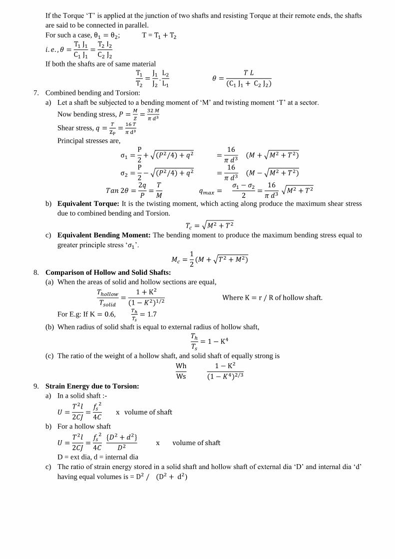
If the Torque ‘T’ is applied at the junction of two shafts and resisting Torque at their remote ends, the shafts

are said to be connected in parallel.

For such a case, ; T =

If both the shafts are of same material

7. Combined bending and Torsion:

a) Let a shaft be subjected to a bending moment of ‘M’ and twisting moment ‘T’ at a sector.

Now bending stress,

Shear stress,

Principal stresses are,

b) Equivalent Torque: It is the twisting moment, which acting along produce the maximum shear stress

due to combined bending and Torsion.

c) Equivalent Bending Moment: The bending moment to produce the maximum bending stress equal to

greater principle stress ‘ ’.

8. Comparison of Hollow and Solid Shafts:

(a) When the areas of solid and hollow sections are equal,

For E.g: If K

(b) When radius of solid shaft is equal to external radius of hollow shaft,

(c) The ratio of the weight of a hollow shaft, and solid shaft of equally strong is

9. Strain Energy due to Torsion:

a) In a solid shaft :-

b) For a hollow shaft

D = ext dia, d = internal dia

c) The ratio of strain energy stored in a solid shaft and hollow shaft of external dia ‘D’ and internal dia ‘d’

having equal volumes is = )

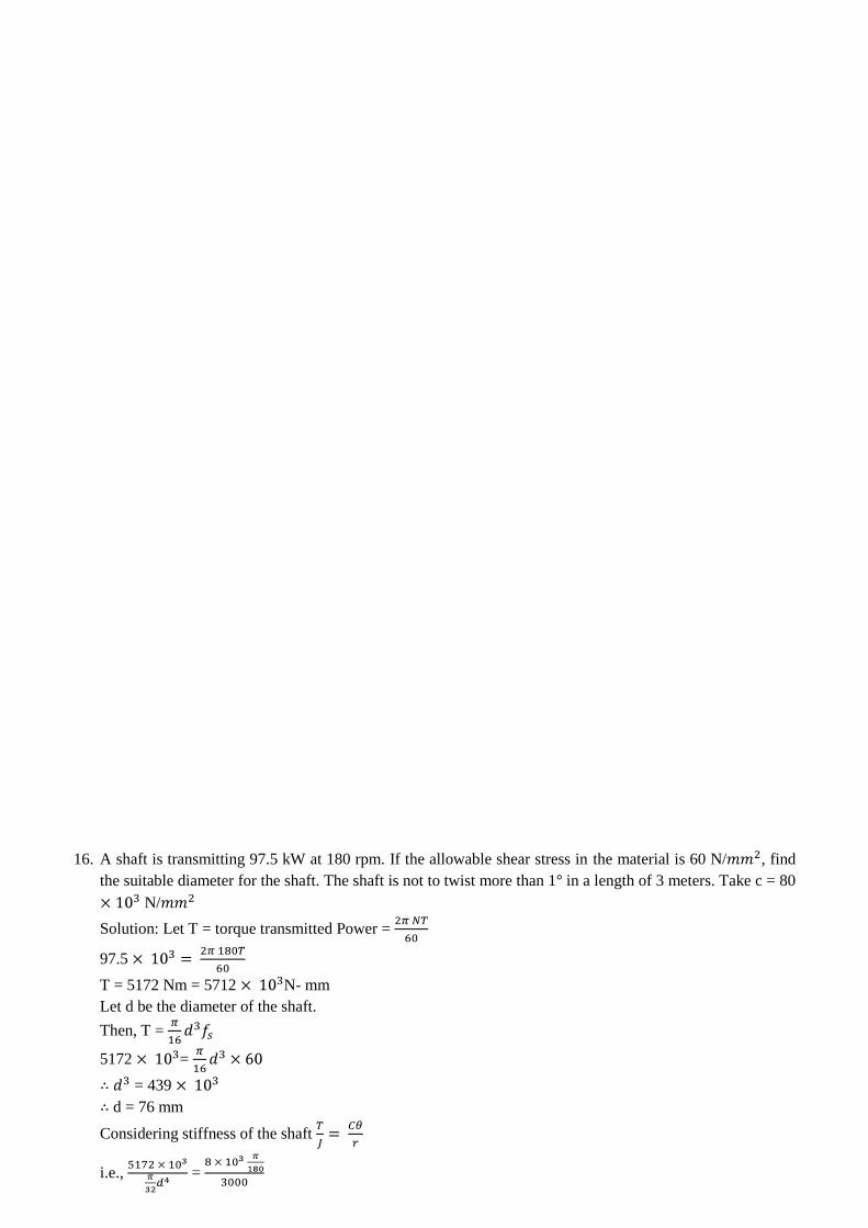
16. A shaft is transmitting 97.5 kW at 180 rpm. If the allowable shear stress in the material is 60 N/ , find

the suitable diameter for the shaft. The shaft is not to twist more than 1 in a length of 3 meters. Take c = 80

N/

Solution: Let T = torque transmitted Power =

97.5

T = 5172 Nm = 5712 N- mm

Let d be the diameter of the shaft.

Then, T =

5172 =

= 439

d = 76 mm

Considering stiffness of the shaft

i.e., =

= 113191150 d = 103(say 105 mm)

We adopt the greater value. i.e., 105 mm.

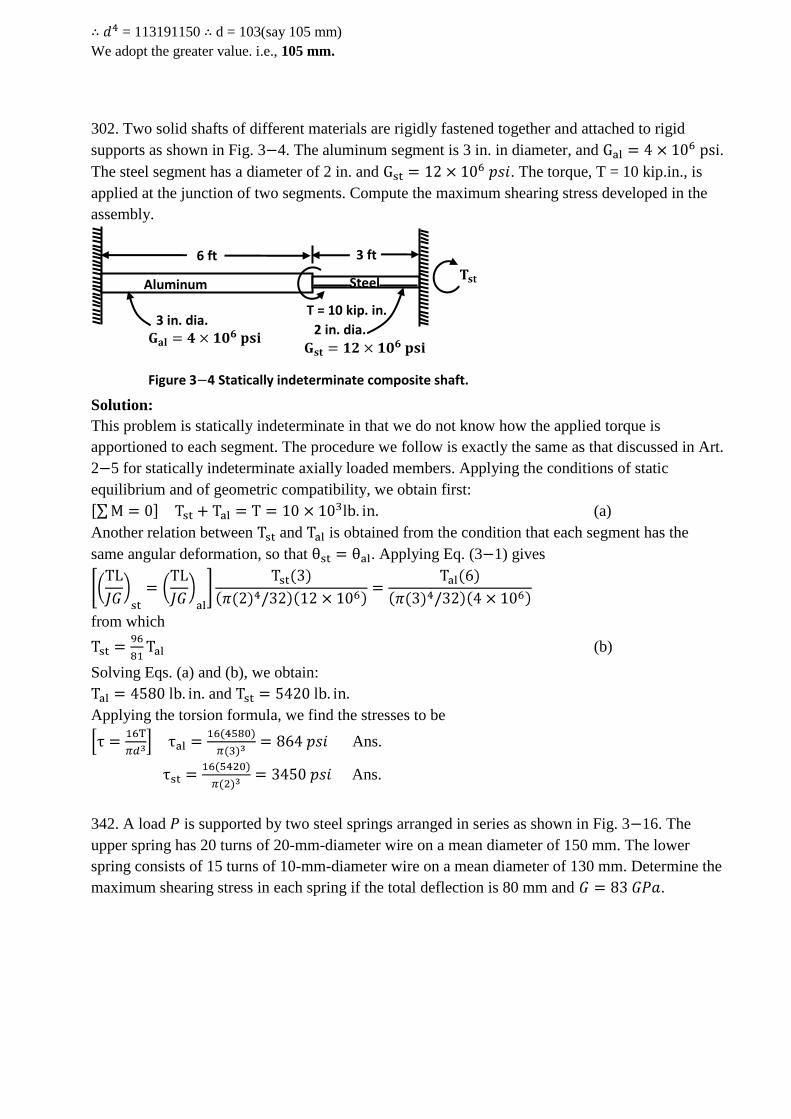
302. Two solid shafts of different materials are rigidly fastened together and attached to rigid

supports as shown in Fig. 3 4. The aluminum segment is 3 in. in diameter, and .

The steel segment has a diameter of 2 in. and . The torque, T = 10 kip.in., is

applied at the junction of two segments. Compute the maximum shearing stress developed in the

assembly.

Solution:

This problem is statically indeterminate in that we do not know how the applied torque is

apportioned to each segment. The procedure we follow is exactly the same as that discussed in Art.

2 5 for statically indeterminate axially loaded members. Applying the conditions of static

equilibrium and of geometric compatibility, we obtain first:

(a)

Another relation between and is obtained from the condition that each segment has the

same angular deformation, so that . Applying Eq. (3 1) gives

from which

(b)

Solving Eqs. (a) and (b), we obtain:

and

Applying the torsion formula, we find the stresses to be

Ans.

Ans.

342. A load is supported by two steel springs arranged in series as shown in Fig. 3 16. The

upper spring has 20 turns of 20-mm-diameter wire on a mean diameter of 150 mm. The lower

spring consists of 15 turns of 10-mm-diameter wire on a mean diameter of 130 mm. Determine the

maximum shearing stress in each spring if the total deflection is 80 mm and .

6 ft 3 ft

Aluminum Steel

3 in. dia.

T = 10 kip. in.

2 in. dia.

Figure 3 4 Statically indeterminate composite shaft.

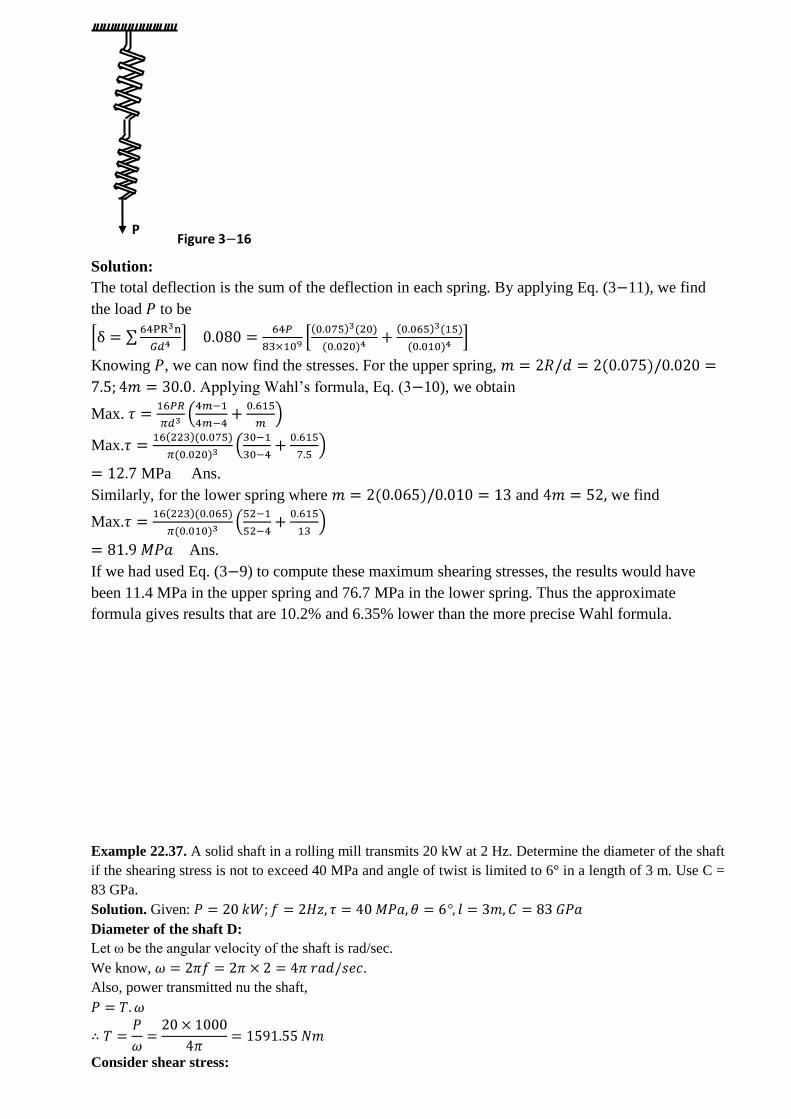
Solution:

The total deflection is the sum of the deflection in each spring. By applying Eq. (3 11), we find

the load to be

Knowing , we can now find the stresses. For the upper spring,

. Applying Wahl’s formula, Eq. (3 10), we obtain

Max.

Max.

MPa Ans.

Similarly, for the lower spring where and we find

Max.

Ans.

If we had used Eq. (3 9) to compute these maximum shearing stresses, the results would have

been 11.4 MPa in the upper spring and 76.7 MPa in the lower spring. Thus the approximate

formula gives results that are 10.2% and 6.35% lower than the more precise Wahl formula.

Example 22.37. A solid shaft in a rolling mill transmits 20 kW at 2 Hz. Determine the diameter of the shaft

if the shearing stress is not to exceed 40 MPa and angle of twist is limited to 6° in a length of 3 m. Use C =

83 GPa.

Solution. Given:

Diameter of the shaft D:

Let ω be the angular velocity of the shaft is rad/sec.

We know, .

Also, power transmitted nu the shaft,

Consider shear stress:

Figure 3 16 P

Consider angle of twist:

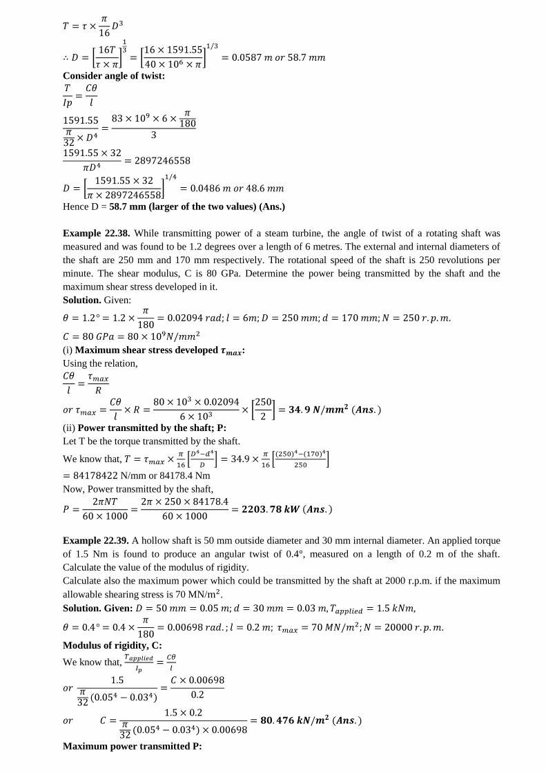
Hence D = 58.7 mm (larger of the two values) (Ans.)

Example 22.38. While transmitting power of a steam turbine, the angle of twist of a rotating shaft was

measured and was found to be 1.2 degrees over a length of 6 metres. The external and internal diameters of

the shaft are 250 mm and 170 mm respectively. The rotational speed of the shaft is 250 revolutions per

minute. The shear modulus, C is 80 GPa. Determine the power being transmitted by the shaft and the

maximum shear stress developed in it.

Solution. Given:

(i) Maximum shear stress developed :

Using the relation,

(ii) Power transmitted by the shaft; P:

Let T be the torque transmitted by the shaft.

We know that,

N/mm or 84178.4 Nm

Now, Power transmitted by the shaft,

Example 22.39. A hollow shaft is 50 mm outside diameter and 30 mm internal diameter. An applied torque

of 1.5 Nm is found to produce an angular twist of 0.4°, measured on a length of 0.2 m of the shaft.

Calculate the value of the modulus of rigidity.

Calculate also the maximum power which could be transmitted by the shaft at 2000 r.p.m. if the maximum

allowable shearing stress is 70 MN/ .

Solution. Given:

Modulus of rigidity, C:

We know that,

Maximum power transmitted P:

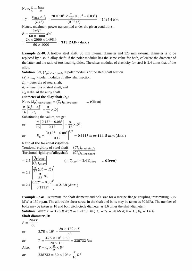
Now,

Hence, maximum power transmitted under the given conditions,

Example 22.40. A hollow steel shaft; 80 mm internal diameter and 120 mm external diameter is to be

replaced by a solid alloy shaft. If the polar modulus has the same value for both, calculate the diameter of

the latter and the ratio of torsional rigidities. The shear modulus of elasticity for steel is 2.4 times that of the

alloy.

Solution. Let, ( = polar modulus of the steel shaft section

= polar modulus of alloy shaft section,

= outer dia of steel shaft,

= inner dia of steel shaft, and

= dia. of the alloy shaft.

Diameter of the alloy shaft :

Now, … (Given)

Substituting the values, we get

Ratio of the torsional rigidities:

Example 22.41. Determine the shaft diameter and bolt size for a marine flange-coupling transmitting 3.75

MW at 150 r.p.m. The allowable shear stress in the shaft and bolts may be taken as 50 MPa. The number of

bolts may be taken as 10 and bolt pitch circle diameter as 1.6 times the shaft diameter.

Solution. Given:

Shaft diameter, D:

Also,

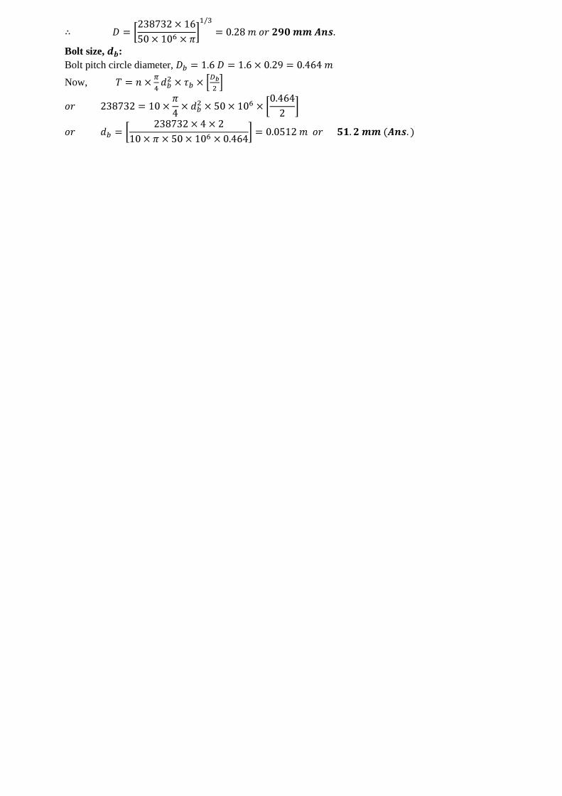
Bolt size, :

Bolt pitch circle diameter,

Now,

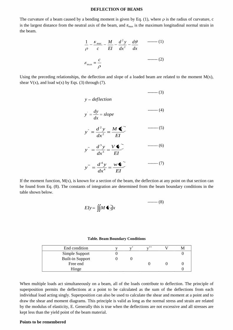
DEFLECTION OF BEAMS

The curvature of a beam caused by a bending moment is given by Eq. (1), where is the radius of curvature, c

is the largest distance from the neutral axis of the beam, and max is the maximum longitudinal normal strain in

the beam.

dx

d

dx

yd

EI

M

c

mac

2

21 ------- (1)

cmax

------- (2)

Using the preceding relationships, the deflection and slope of a loaded beam are related to the moment M(x),

shear V(x), and load w(x) by Eqs. (3) through (7).

deflectiony

------- (3)

slopedx

dyy '

------- (4)

EI

xM

dx

ydy

2

2''

------- (5)

EI

xV

dx

ydy

3

3'''

------- (6)

EI

xw

dx

ydy

4

4''''

------- (7)

If the moment function, M(x), is known for a section of the beam, the deflection at any point on that section can

be found from Eq. (8). The constants of integration are determined from the beam boundary conditions in the

table shown below.

dxxMEIy

------- (8)

Table. Beam Boundary Conditions

End condition y y’ y’’ V M

Simple Support 0 0

Built-in Support 0 0

Free end 0 0 0

Hinge 0

When multiple loads act simultaneously on a beam, all of the loads contribute to deflection. The principle of

superposition permits the deflections at a point to be calculated as the sum of the deflections from each

individual load acting singly. Superposition can also be used to calculate the shear and moment at a point and to

draw the shear and moment diagrams. This principle is valid as long as the normal stress and strain are related

by the modulus of elasticity, E. Generally this is true when the deflections are not excessive and all stresses are

kept less than the yield point of the beam material.

Points to be remembered

A L B

A L B

M

A B

E

D

1. Relation between curvature, slope and deflection:

a) Curvature - - - - - for ve B.M

or EI / = M - - - - - for B.M is + ve

b) Slope θ = dy / dx radians EIθ = EI. dy / dx =

c) Deflection = y, EIy =

d) EI y / = dM / dx = + F

e) EI y / = dF / dx = + W

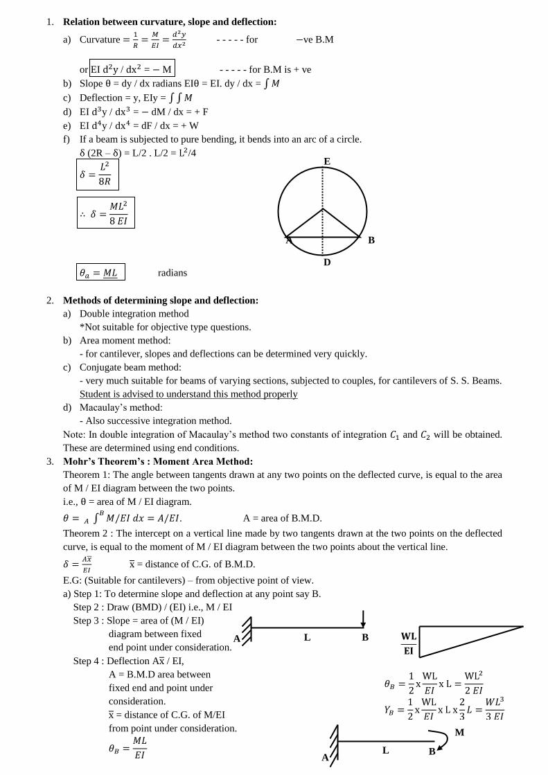
f) If a beam is subjected to pure bending, it bends into an arc of a circle.

δ (2R – δ) = L/2 . L/2 = /4

radians

2. Methods of determining slope and deflection:

a) Double integration method

*Not suitable for objective type questions.

b) Area moment method:

- for cantilever, slopes and deflections can be determined very quickly.

c) Conjugate beam method:

- very much suitable for beams of varying sections, subjected to couples, for cantilevers of S. S. Beams.

Student is advised to understand this method properly

d) Macaulay’s method:

- Also successive integration method.

Note: In double integration of Macaulay’s method two constants of integration and will be obtained.

These are determined using end conditions.

3. Mohr’s Theorem’s : Moment Area Method:

Theorem 1: The angle between tangents drawn at any two points on the deflected curve, is equal to the area

of M / EI diagram between the two points.

i.e., θ = area of M / EI diagram.

. A = area of B.M.D.

Theorem 2 : The intercept on a vertical line made by two tangents drawn at the two points on the deflected

curve, is equal to the moment of M / EI diagram between the two points about the vertical line.

= distance of C.G. of B.M.D.

E.G: (Suitable for cantilevers) – from objective point of view.

a) Step 1: To determine slope and deflection at any point say B.

Step 2 : Draw (BMD) / (EI) i.e., M / EI

Step 3 : Slope = area of (M / EI)

diagram between fixed

end point under consideration.

Step 4 : Deflection A / EI,

A = B.M.D area between

fixed end and point under

consideration.

= distance of C.G. of M/EI

from point under consideration.

4. Maxwell’s Law of Reciprocal Deflections:

Consider cantilever beam AB. Let ‘C’ be an intermediate point. Then the deflection at ‘C’ due to a point

load ‘P’ at B say , is equal to deflection at ‘B’ due to a point load ‘P’ at C i.e.,

∴

Slope and deflection of beams

SL No. 1

Type of Loading

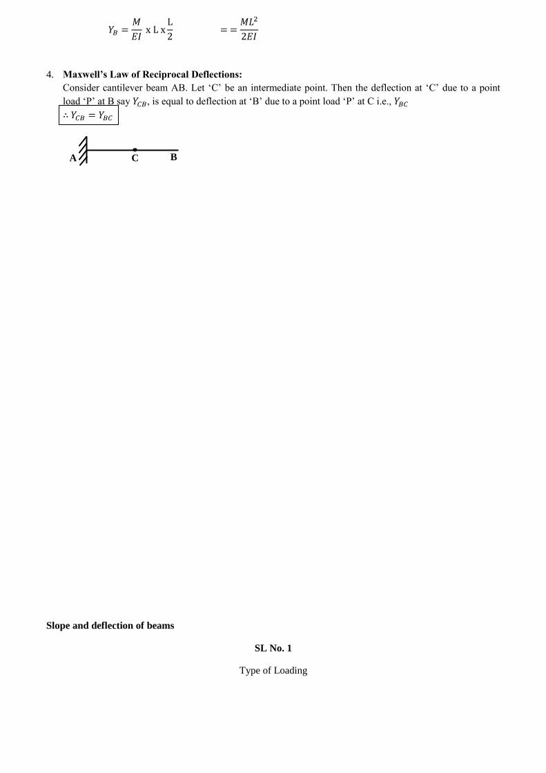
A C B

Maximum Bending Moment

Slope

Maximum Deflection

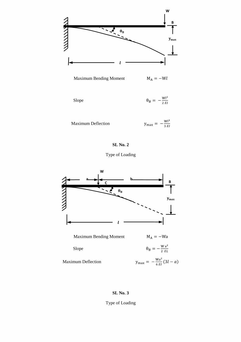
SL No. 2

Type of Loading

Maximum Bending Moment

Slope

Maximum Deflection

SL No. 3

Type of Loading

b B

A

a C

W

W

B A

Maximum Bending Moment where W = ( total load on the

cantilever)

Slope

Maximum Deflection

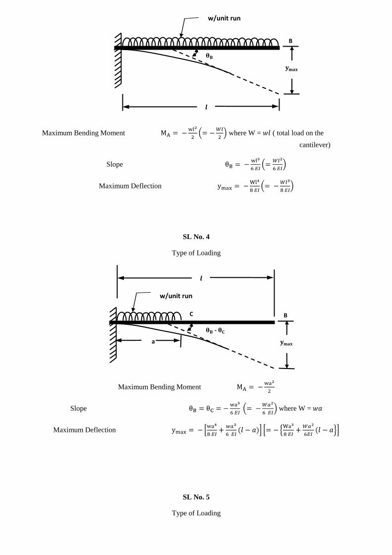
SL No. 4

Type of Loading

Maximum Bending Moment

Slope where W =

Maximum Deflection

SL No. 5

Type of Loading

B A

-

w/unit run

a

C

B A

w/unit run

Maximum Bending Moment

Slope

Maximum Deflection

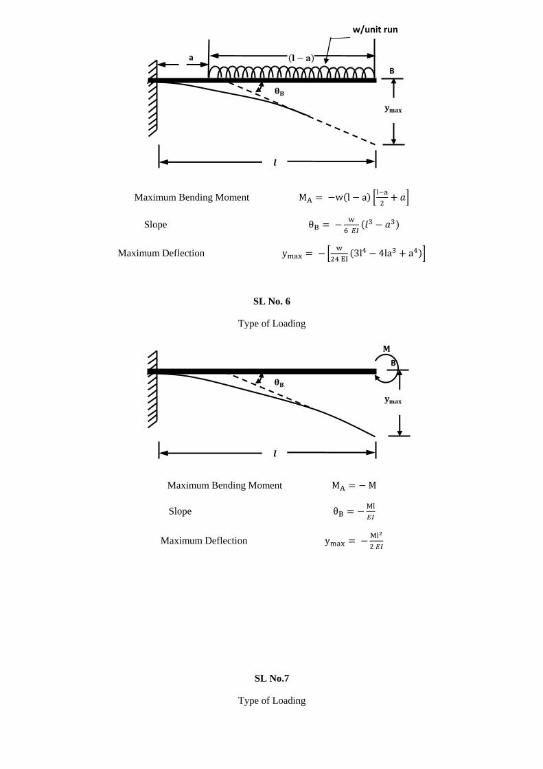
SL No. 6

Type of Loading

Maximum Bending Moment

Slope

Maximum Deflection

SL No.7

Type of Loading

B A

B A

w/unit run

a

Maximum Bending Moment

Slope

Maximum Deflection

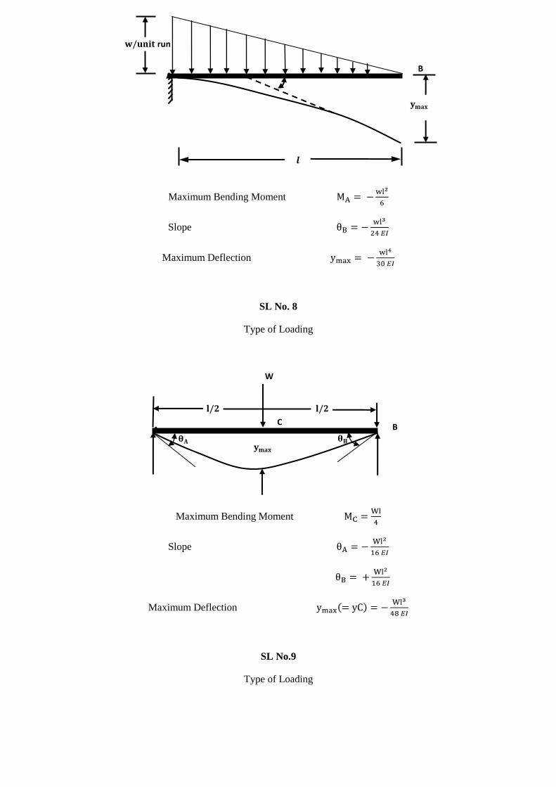
SL No. 8

Type of Loading

Maximum Bending Moment

Slope

Maximum Deflection

SL No.9

Type of Loading

C B A

W

B A

run

Maximum Bending Moment

Slope

Maximum Deflection

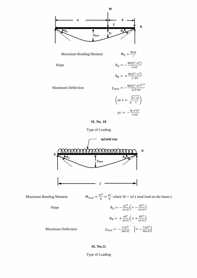
SL No. 10

Type of Loading

Maximum Bending Moment where W = ( total load on the beam )

Slope

Maximum Deflection

SL No.11

Type of Loading

B A

w/unit run

C B A

W

Maximum Bending Moment

Slope

Maximum Deflection

( at x = 0∙519 and A )

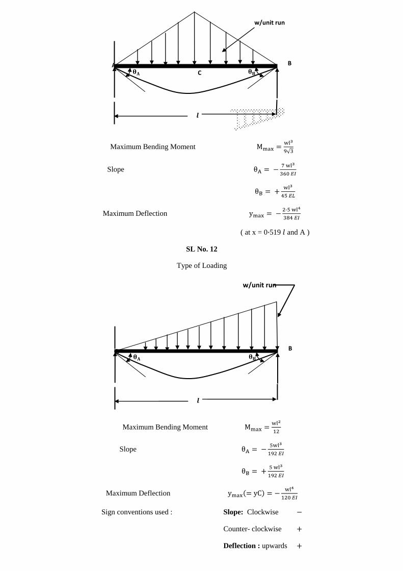
SL No. 12

Type of Loading

Maximum Bending Moment

Slope

Maximum Deflection

Sign conventions used : Slope: Clockwise

Counter- clockwise

Deflection : upwards

B A

w/unit run

B A C

w/unit run

Downward

49. A strut of length has its ends built into a material which exerts a constraining couple equal to k times the

angular rotation in radians. Show that the buckling load is given by the equation

tan where

Solution: = - M - Py

Y +

)y =

y = sin mx + cos mx -

At x = 0, y = 0; 0 = =

= m cos mx - m sin mx

At x = 0, = - ; - = m

= -

At x = , = 0

0 = m cos - m sin

= tan

(i.e.,) = tan

tan = - .

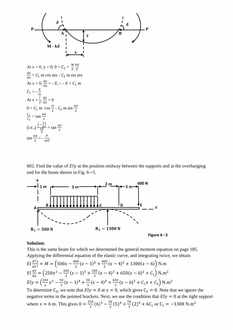
602. Find the value of at the position midway between the supports and at the overhanging

end for the beam shown in Fig. 6 5.

Solution:

This is the same beam for which we determined the general moment equation on page 185.

Applying the differential equation of the elastic curve, and integrating twice, we obtain

N.m

N.

N.

To determine , we note that at , which gives . Note that we ignore the

negative terms in the pointed brackets. Next, we use the condition that at the right support

where . This gives or N.

600 N 2 m

2 m 3 m 1 m

y

A B C D E

Figure 6 5

x

y

P B A

P

M - k

Finally, to obtain the midspan deflection, we substitute in the deflection equations for

segment obtained by ignoring negative values of the bracketed terms and .

We obtain

N. Ans.

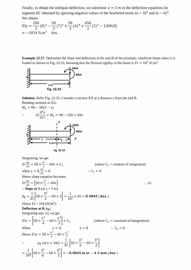
Example 22.27. Determine the slope and deflection at the end B of the prismatic cantilever beam when it is

loaded as shown in Fig. 22.33, knowing that the flexural rigidity of the beam is .

Solution. Refer Fig. 22.33. Consider a section XX at a distance x from the end B.

Bending moment at XX,

Integrating, we get

(where = constant of integration)

when ∴

Hence slope equation becomes,

… (i)

∴ Slope at B (at x = 3 m)

(Since EI = 104 kN/ )

Deflection at B, :

Integrating eqn. (i), we get

When

Hence

B

50kN

90kN

3 m

A

X

Fig. 22.34

B

50kN

90kN

3 m

A

Fig. 22.33

D

W W

(c) B.M. Diagram

A B C a a

W

W

= W = W

(a) Beam

(b) S.F. Diagram

Fig. 22.38

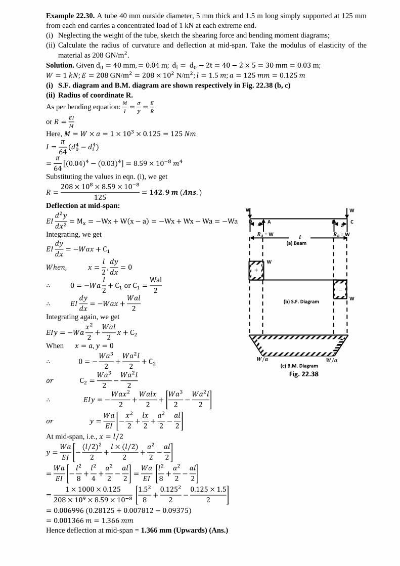
Example 22.30. A tube 40 mm outside diameter, 5 mm thick and 1.5 m long simply supported at 125 mm

from each end carries a concentrated load of 1 kN at each extreme end.

(i) Neglecting the weight of the tube, sketch the shearing force and bending moment diagrams;

(ii) Calculate the radius of curvature and deflection at mid-span. Take the modulus of elasticity of the

material as 208 GN/ .

Solution. Given

GN/ N/

(i) S.F. diagram and B.M. diagram are shown respectively in Fig. 22.38 (b, c)

(ii) Radius of coordinate R.

As per bending equation:

or

Here,

Substituting the values in eqn. (i), we get

Deflection at mid-span:

Integrating, we get

Integrating again, we get

When

At mid-span, i.e.,

Hence deflection at mid-span = 1.366 mm (Upwards) (Ans.)

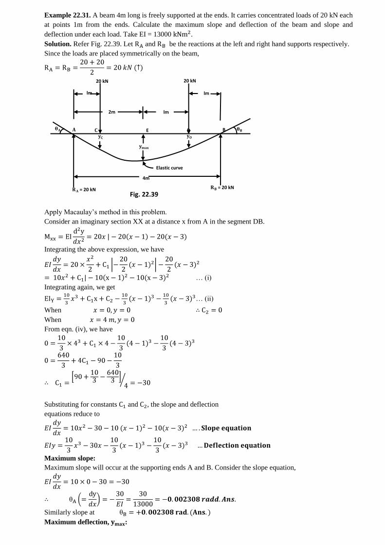
Example 22.31. A beam 4m long is freely supported at the ends. It carries concentrated loads of 20 kN each

at points 1m from the ends. Calculate the maximum slope and deflection of the beam and slope and

deflection under each load. Take EI = 13000 .

Solution. Refer Fig. 22.39. Let and be the reactions at the left and right hand supports respectively.

Since the loads are placed symmetrically on the beam,

Apply Macaulay’s method in this problem.

Consider an imaginary section XX at a distance x from A in the segment DB.

Integrating the above expression, we have

… (i)

Integrating again, we get

… (ii)

When ∴

When

From eqn. (iv), we have

Substituting for constants and , the slope and deflection

equations reduce to

Maximum slope:

Maximum slope will occur at the supporting ends A and B. Consider the slope equation,

Similarly slope at

Maximum deflection, :

= 20 kN

E D B

4m

2m lm

lm lm

Elastic curve

= 20 kN

20 kN 20 kN

Fig. 22.39

For obtaining maximum deflection, we should first determine the position where slope is zero. Considering

the slope equation we have:

[Since the term 10 will be negative for the segment CD and hence

neglected]

or

from A.

Now in order to determine maximum deflection, put x = 2m in the deflection equation

Hence = 2.82 mm (downwards)

Slope under the load 20 kN at C, :

Substituting x = 1 m in the slope equation, we get

Slope under the load 20 kN at D, :

Substituting x = 3 m in the slope equation, we get

Deflection under the load 20 kN at C :

Substituting x = 1, m in the deflection equation, we get

Hence 2.05 mm (downwards) (Ans.)

Deflection under the load 20 kN At D, :

Hence = 2.05 mm (downwards) (Ans.)

Example 22.50. A simply supported beam is subjected to a single force P at a distance b from one of the

supports. Obtain the expression for the deflection under the load using castigliano’s theorem. How do you

calculate deflection at the mid-point of the beam?

Solution. Let load P acts at a distance b from the support B, and l be the total length of the beam.

Reaction at A, , and

Reaction at B,

Strain energy stored by beam AB,

U = Strain energy stored by AC ( + strain energy stored by BC ( )

Deflection under the load (Ans.)

Deflection at the mid-span of the beam can be found by Macaulay’s method.

By Macaulay’s method, deflection at any section is given by

Where y is deflection at any distance x from the support.

At at mid-span,

P

B A

C

Fig. 22.49

MOHR’S CIRCLE

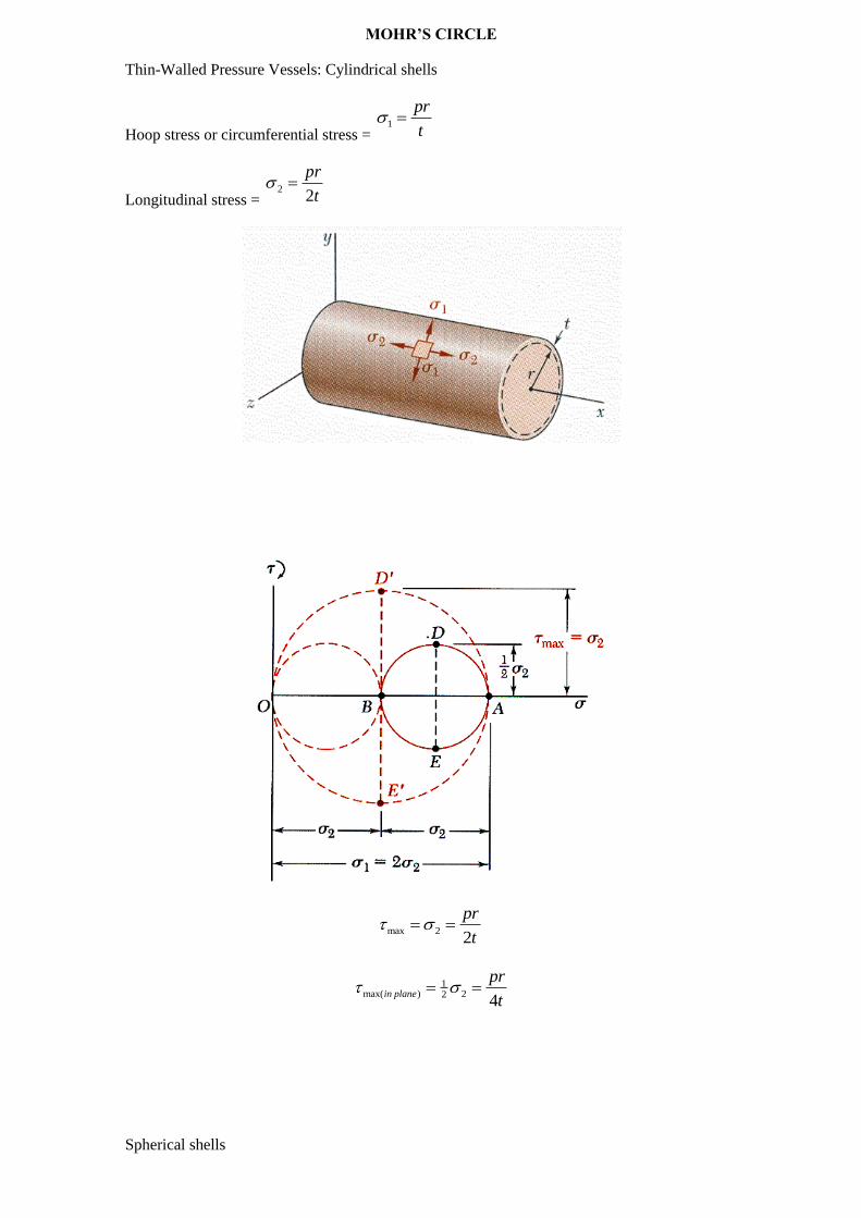
Thin-Walled Pressure Vessels: Cylindrical shells

Hoop stress or circumferential stress = 1

pr

t

Longitudinal stress = 2

2

pr

t

max 22

pr

t

1max( ) 22

4in plane

pr

t

Spherical shells

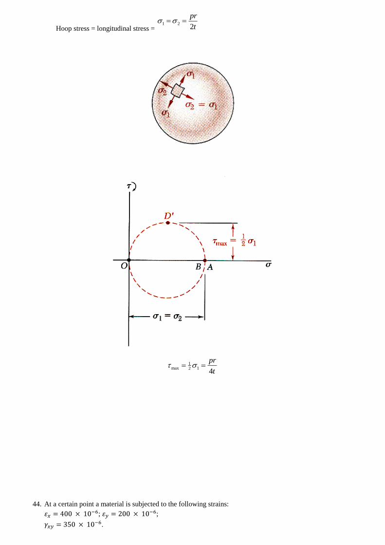
Hoop stress = longitudinal stress = 1 2

2

pr

t

1max 12

4

pr

t

44. At a certain point a material is subjected to the following strains:

; ;

.

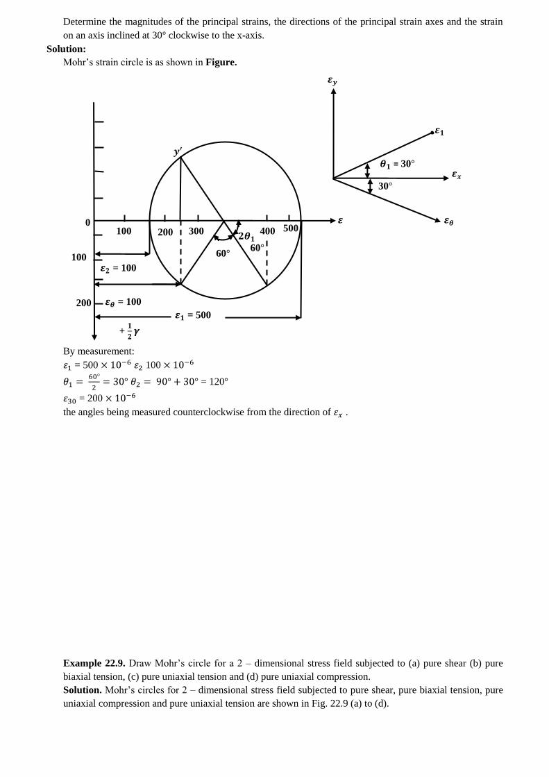
Determine the magnitudes of the principal strains, the directions of the principal strain axes and the strain

on an axis inclined at 30 clockwise to the x-axis.

Solution:

Mohr’s strain circle is as shown in Figure.

By measurement:

= 500 100

= 120

= 200

the angles being measured counterclockwise from the direction of .

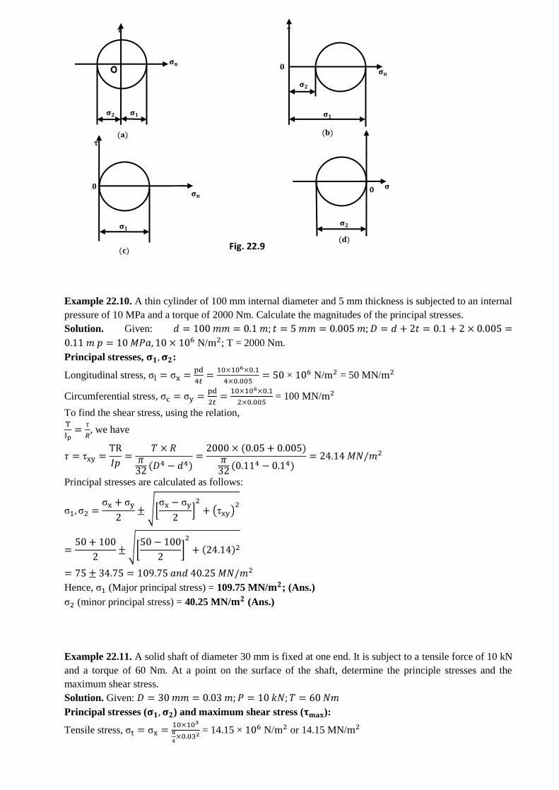
Example 22.9. Draw Mohr’s circle for a 2 – dimensional stress field subjected to (a) pure shear (b) pure

biaxial tension, (c) pure uniaxial tension and (d) pure uniaxial compression.

Solution. Mohr’s circles for 2 – dimensional stress field subjected to pure shear, pure biaxial tension, pure

uniaxial compression and pure uniaxial tension are shown in Fig. 22.9 (a) to (d).

0

100

200

100 200 300 400 500

= 500

= 100

= 100

60 60

+

= 30

30

Example 22.10. A thin cylinder of 100 mm internal diameter and 5 mm thickness is subjected to an internal

pressure of 10 MPa and a torque of 2000 Nm. Calculate the magnitudes of the principal stresses.

Solution. Given:

N/ ; T = 2000 Nm.

Principal stresses, :

Longitudinal stress, × N/ = 50 MN/

Circumferential stress, = 100 MN/

To find the shear stress, using the relation,

, we have

Principal stresses are calculated as follows:

Hence, (Major principal stress) = 109.75 MN/ ; (Ans.)

(minor principal stress) = 40.25 MN/ (Ans.)

Example 22.11. A solid shaft of diameter 30 mm is fixed at one end. It is subject to a tensile force of 10 kN

and a torque of 60 Nm. At a point on the surface of the shaft, determine the principle stresses and the

maximum shear stress.

Solution. Given:

Principal stresses ( ) and maximum shear stress ( ):

Tensile stress, = 14.15 × N/ or 14.15 MN/

τ

τ

τ

Fig. 22.9

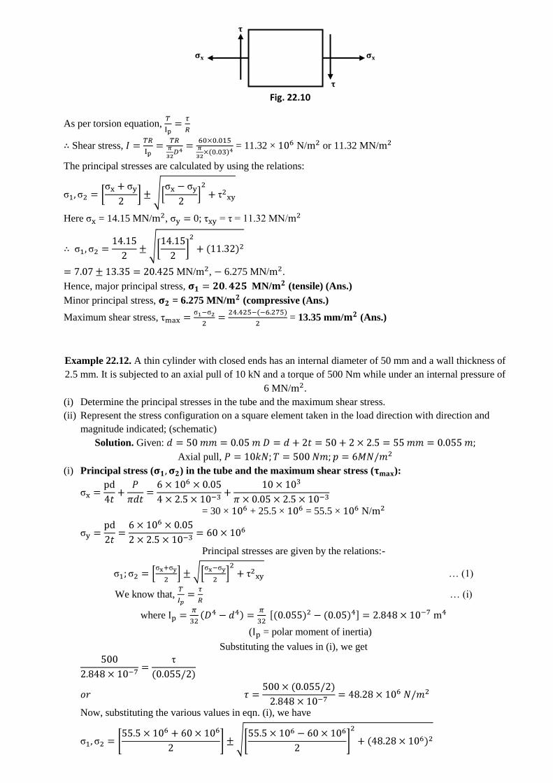
As per torsion equation,

∴ Shear stress, = 11.32 × N/ or 11.32 MN/

The principal stresses are calculated by using the relations:

Here = 14.15 MN/ , 0; = τ = 11.32 MN/

MN/ , 6.275 MN/ .

Hence, major principal stress, MN/ (tensile) (Ans.)

Minor principal stress, = 6.275 MN/ (compressive (Ans.)

Maximum shear stress, = 13.35 mm/ (Ans.)

Example 22.12. A thin cylinder with closed ends has an internal diameter of 50 mm and a wall thickness of

2.5 mm. It is subjected to an axial pull of 10 kN and a torque of 500 Nm while under an internal pressure of

6 MN/ .

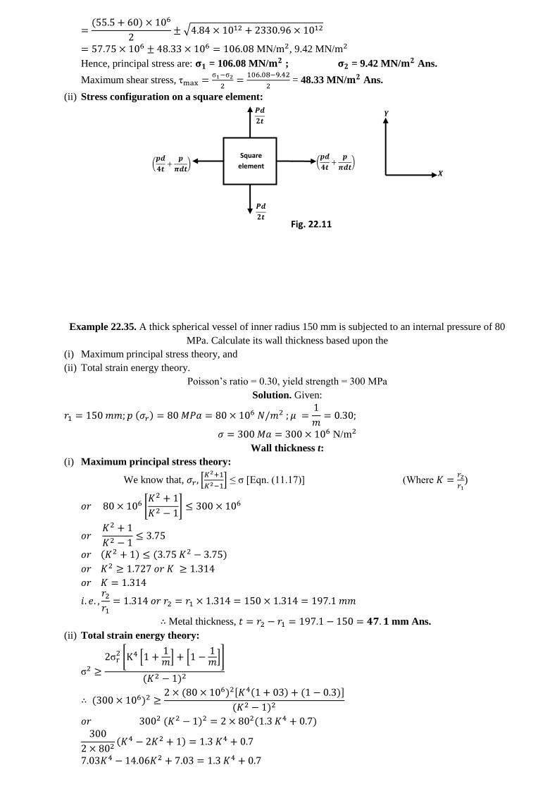
(i) Determine the principal stresses in the tube and the maximum shear stress.

(ii) Represent the stress configuration on a square element taken in the load direction with direction and

magnitude indicated; (schematic)

Solution. Given:

Axial pull,

(i) Principal stress ( ) in the tube and the maximum shear stress ( ):

= 30 × + 25.5 × = 55.5 × N/

Principal stresses are given by the relations:-

… (1)

We know that, … (i)

where

( = polar moment of inertia)

Substituting the values in (i), we get

Now, substituting the various values in eqn. (i), we have

Fig. 22.10

MN/ , 9.42 MN/

Hence, principal stress are: = 106.08 MN/ ; = 9.42 MN/ Ans.

Maximum shear stress, = 48.33 MN/ Ans.

(ii) Stress configuration on a square element:

Example 22.35. A thick spherical vessel of inner radius 150 mm is subjected to an internal pressure of 80

MPa. Calculate its wall thickness based upon the

(i) Maximum principal stress theory, and

(ii) Total strain energy theory.

Poisson’s ratio = 0.30, yield strength = 300 MPa

Solution. Given:

N/

Wall thickness t:

(i) Maximum principal stress theory:

We know that, ≤ σ [Eqn. (11.17)] (Where )

∴ Metal thickness, mm Ans.

(ii) Total strain energy theory:

Square

element

Fig. 22.11

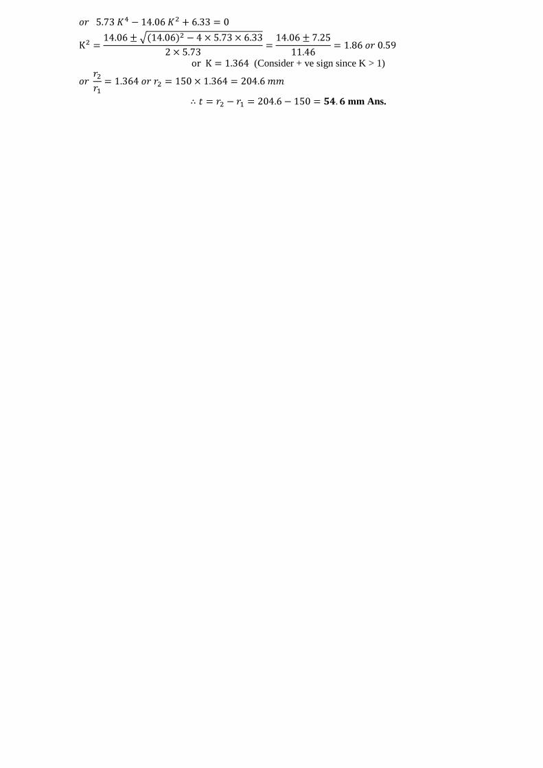
(Consider + ve sign since K > 1)

mm Ans.