THE CENTRE FOR MARKET AND PUBLIC ORGANISATION

Centre for Market and Public Organisation Bristol Institute of Public Affairs

University of Bristol 2 Priory Road

Bristol BS8 1TX http://www.bristol.ac.uk/cmpo/

Tel: (0117) 33 10799 Fax: (0117) 33 10705

E-mail: cmpo-admin@bristol.ac.uk The Centre for Market and Public Organisation (CMPO) is a leading research centre, combining expertise in economics, geography and law. Our objective is to study the intersection between the public and private sectors of the economy, and in particular to understand the right way to organise and deliver public services. The Centre aims to develop research, contribute to the public debate and inform policy-making. CMPO, now an ESRC Research Centre was established in 1998 with two large grants from The Leverhulme Trust. In 2004 we were awarded ESRC Research Centre status, and CMPO now combines core funding from both the ESRC and the Trust.

ISSN 1473-625X

Incentives in the Public Sector: Evidence from a Government Agency

Simon Burgess, Carol Propper, Marissa Ratto and Emma Tominey

August 2011

Working Paper No. 11/265

CMPO Working Paper Series No. 11/265

Incentives in the Public Sector: Evidence from a Government Agency

Simon Burgess1, Carol Propper2, Marisa Rattoand Emma Tominey

3

4

1University of Bristol, CMPO and CEPR 2University of Bristol, CMPO, Imperial College London and CEPR

3Université Paris-Dauphine (SDFi) and CMPO 4

University of York and CMPO

August 5th 2011 Abstract This paper addresses a lack of evidence on the impact of performance pay in the public sector by evaluating a pilot scheme of incentives in a major government agency. The incentive scheme was based on teams and covered quantity and quality targets, measured with varying degrees of precision. We use data from the agency’s performance management system and personnel records plus matched labour market data. We focus on three main issues: whether performance pay matters for public service worker productivity, what the team basis of the scheme implies, and the impact of the differential measurement precision. We show that the use of performance pay had no impact at the mean, but that there was significant heterogeneity of response. This heterogeneity was patterned as one would expect from a free rider versus peer monitoring perspective. We found that the incentive had a substantial positive effect in small teams, and a negative response in large teams. We found little impact of the scheme on quality measures, which we interpret as due to the differential measurement technology. We show that the scheme in small teams had non-trivial effects on output, and our estimates suggest that the use of incentive pay is much more cost effective than a general pay rise.

Keywords: Incentives, Public Sector, Teams, Performance, Personnel Economics JEL Classification: J33, J45, D23 Electronic version:

www.bristol.ac.uk/cmpo/publications/papers/2011/wp265.pdf

Acknowledgements This work was funded by the Department for Work and Pensions (DWP), the Public Sector Productivity Panel, the Evidence-based Policy Fund and the Leverhulme Trust through CMPO. The views in the paper do not necessarily reflect those of these organisations. Thanks to individuals in the DWP for helping to secure the data for us, particularly Storm Janeway, Stavros Flouris and Phil Parramore. Thanks for comments to seminar participants at Bristol, the Public Economics Working Group Conference at Warwick, the IIES at Stockholm, University of Melbourne, HM Treasury, CPB in The Hague, Tinbergen Institute and Department for Work and Pensions.

Address for correspondence CMPO, Bristol Institute of Public Affairs University of Bristol 2 Priory Road Bristol BS8 1TX Simon.burgess@bristol.ac.uk www.bristol.ac.uk/cmpo/

3

Governments employ a lot of people. The productivity of these workers, forming such a

substantial fraction of the labour force (15% in the US, more than are employed in

manufacturing at 13%) is therefore a major issue and many governments have an explicit

agenda of improving the efficiency of public service delivery1

. One method which has

received considerable attention is the use of explicit financial incentives. Early examples

include Osborne and Gaebler (1993) “Reinventing Government”, promoted by Vice-

President Gore in the USA and the Job Partnership Agency Scheme in the USA in the 1980s

(Barnow 2000, Heckman et al. 1996). More lately, there has been considerable interest in

performance related pay for teachers and public sector doctors (e.g. Lavy 2009, Gravelle et

al. 2010).

Theorists have addressed the role of such incentives in the public sector, drawing attention to

a set of features such as multiple tasks, multiple principals and missions, all of which suggest

that even if there is no difference in the inputs of the production process between the private

and public sector, there are some specific features related to outputs and to the way public

sector agencies are structured which mean that incentives might be expected to have different

consequences in public organisations (e.g. Dixit 2002, Prendergast 1999, Baker 2002,

Francois 2000, Besley and Ghatak 2005). However, despite the interest (Burgess and Ratto

2003), the empirical evidence on the use of incentives in the public sector is still quite scant

and a recent review concluded that there are relatively few estimates from which causal

inferences can be made (Bloom and Van Reenen 2010).

This paper aims to fill this gap. In a search for greater public sector productivity, the

government of the UK in the late 1990s piloted the use of financial incentives for lower level

bureaucrats. As part of this programme they introduced a pilot programme of the use of team-

based financial incentives in a large UK public agency. The agency, Jobcentre Plus, was one

of the main government agencies dealing with the public: its role was to place the

unemployed into jobs and administer welfare benefits. In contrast with many schemes in the

private sector, the incentive scheme we analyse was exogenously imposed on the

organisation, as it was part of a wider government experiment with incentive pay (Makinson

2000). In addition, it was a team based performance pay scheme: workers were rewarded on

the basis of team rather than individual production.

1 The World Development Report (2003) highlights that concern is not limited to developed countries.

4

The specific nature of the incentive scheme allows us to investigate three key issues. First,

what is the impact of an explicit financial incentive scheme on public sector workers? Dixit’s

(2002) review of theoretical contributions suggests that such incentives may be counter-

productive. Evidence on the effectiveness of incentive schemes in the public sector is mixed.

Kahn, Silva and Ziliak (2001) examine a reform to the Brazilian tax collection authority

which paid financial incentives based on individual and team performance in detecting and

fining tax evaders. Amounts involved were substantial, frequently providing bonuses over

twice mean annual salary. Authors find a dramatic effect, with fine collections per inspection

75% higher than in the counter-factual. Lavy (2009) found that teacher incentives to improve

pupil performance in maths and English significantly raised student outcomes. Baiker and

Jacobson (2007) in a study of the police where participants were able to keep a proportion of

the value of drug-related asset seizes found significant effect of the incentives, documenting

an increase in heroin related drug offenses and even a rise in the price of heroin. But counter-

examples exist – for example Mullen et al (2010) found little effect of pay for performance

on the quality of medical care.

Second, what is the impact of a team-based incentive scheme? Economists have typically

been skeptical of a team basis for obvious free-rider problems and free rider effects have been

found (e.g. Gaynor and Pauly 1990, Gaynor et al. 2004, Bhattacherjee 2005) 2

. On the other

hand, Burgess et al. (2010) find that even in quite large teams, a team-based incentive scheme

in the UK Customs and Excise raised the productivity of agency workers. Knez and Simester

(2001) argue that peer monitoring outweighed free riding effects in a scheme in Continental

Airlines which had large teams and Hamilton, Nickerson and Owan (2003) conclude

similarly for a garment factory in California. The incentive scheme we analyze was

introduced across teams of very different structures, so allowing us to quantify the effect of

team size.

Third, how do workers respond to relative task measurement precision in an explicitly multi-

tasking environment? Although the implications of multi-tasking for scheme design are a

major part of the literature on incentives, there is very little empirical evidence on the

importance of the precision with which targeted outcomes are measured. Gaynor and Pauly

2 Holmström (1982) provides the formalisation.

5

(1990) investigate the productive efficiency of physicians practicing in groups of medical

partnerships, with differing compensation structures. They showed that output was greater

where compensation was more directly related to productivity. The incentive scheme we

study here incorporated five targets covering most of the tasks of the agency. In practice, only

4 of these were measured. Of these, one was defined in terms of quantity of output, three

were defined in terms of quality. The quantity target was measured with considerable

precision as it was a weighted count of every client placed in a job, while the quality targets

were measured with considerably less precision. We can therefore evaluate the impact of

measurement precision.

The scheme was designed to be a randomised control trial. However, we only observe data

for the year that the scheme was in operation, so we compare the treated and controls during

that year. Our results suggest that the overall impact of the scheme was zero. However, we

also find significant heterogeneity of response that fits with important free rider effects in

production. The impact of the incentive scheme was greatest in small offices and in districts

composed of fewer offices. Thus while some mechanism such as peer monitoring does

overcome the free-riding problem in small teams, it appears not to do so in large teams.

Finally, whilst quantity increased, the scheme had little effect on the quality of service. This

suggests that relative measurement precision in a multi-tasking context is important. Overall,

the scheme design was not optimal in a number of ways which we briefly discuss in our

conclusions.

Section 1 describes the nature of the organisation and the incentive scheme. Section 2

introduces the data and sets out our modelling framework and identification strategy. Section

3 presents our estimation results and robustness checks. In section 4 we use these to evaluate

the scheme. Section 5 concludes.

1. The Incentive Scheme

1.1 The Structure of Jobcentre Plus

The primary roles of Jobcentre Plus (JP) were to help place people into jobs and to administer

benefits. It was launched in October 2001, amalgamating the functions of two agencies: the

Benefits Agency (BA), responsible for administering benefits to the unemployed, lone

6

parents and others, and the Employment Service (ES), responsible for job placement. The

method of delivering these services also began to change with 56 new ‘Pathfinder’ offices

providing an integrated service, combining the work of the original, separate, benefits offices

and employment offices. This process of change was slow, and most offices at the time of our

study – there were 1464 in total – remained single service providers as ex-BA or ex-ES

offices. More Pathfinder offices were created through the year of the pilot scheme.

There were few operational links between offices in a district - that is, the work of non-

Pathfinder offices was largely unaffected by the presence of Pathfinder offices in the district,

and different offices were largely self-contained. The districts with the new-style offices were

designated Pathfinder districts. At April 2002, these made up 17 out of 90 districts in total.

1.2 The Nature of the Incentive Scheme

The initial drive for the introduction of financial incentives was political, originating in the

White Paper “Modernising Government” (1999). This was followed up in the Makinson

report (2000) for the Public Sector Productivity Panel, advocating incentive schemes for front

line government workers. This study evaluates one of these schemes3

. The pilot incentive

scheme ran from April 2002 to March 2003. The main relevant features of the scheme are as

follows.

1.2.1 Teams

This was a team-based scheme. The rationale for designing a team-based rather than an

individual-based incentive scheme was to promote cooperation among workers4

3 See Burgess et al. (2010) for the evaluation of another, implemented in the UK HMCE (Her Majesty’s Custom and Excise).

. The unit

chosen as the basis for the team was the district. The targets were defined at district level, all

workers in the district got the bonus if the target was hit, and the district manager was

responsible for achieving the target. So the team was defined by the reward system (the

targets and the bonus were set at district level) and not by the production function. These

teams were large - there were only 90 districts covering the whole of the country, varying in

4 There were also two more practical reasons. Discussions with the designers revealed that it would have been very hard to get the Unions’ consent for the introduction of performance related pay based on individual output. There were also some output measurability issues: some of the output measures relate to the quality of the service provided by the agency, and these measures are only available at the aggregate level of districts (see also below).

7

size from 5 to 39 offices in the team, and from 264 and 1535 people within a team5

. The 17

Pathfinder districts were incentivsed.

1.2.2 Threshold incentive payment

In common with many schemes, the form adopted was a step function, based on a threshold

level of performance. Workers were paid a straight salary up to the threshold, the bonus was

paid for hitting the threshold, and then there was no further increase in remuneration for

further output. Thus incentives are very sharp at output levels just below the threshold but

weaker further below or above. The scheme was originally set up to offer 1% of salary for

each target hit (conditional on teams achieving at least 2 targets) plus an additional 2.5% if all

were hit, though the details evolved slightly through the period of the pilot6. The targets for

the incentivised districts were set as percentage increases on the previous year’s

achievements7

. The incentivized districts were grouped into two categories. Band A districts,

which contained up to 20% of Pathfinder offices over the total number of offices, and B

districts, with 21% or more of Pathfinder offices. Two different target levels were applied to

the two categories - for Band A districts the incentive target consisted of 5% increase in the

baseline output target, whereas for Band B districts it was a 7.5% increase.

1.2.3 Multiple targets

One central issue in the design of incentive structures is the importance of multi-tasking. In

particular, a trade-off between quantity produced and quality is often crucial8

5 Knez and Simester (2001) analyse the impact of incentives within big teams.

. This incentive

scheme recognized that and included targets for five different functions, which together

measure both quantity and quality. Discussed in detail below these are job placements

(quantity), customer service, employer service, other business delivery functions, and

reducing benefit calculation error and fraud (all quality). The specific activities involved, and

the ease with which each target was measured differ widely across these five targets. For

6 The final bonus was actually based around standard rates, which varied with the job grade per target hit. If all five targets were achieved there was an extra 50% of the standard rate. This means that if all five targets were hit, a band A worker would earn an extra £750, whereas a band G job would get £3,750 more. This represents around 7.5 and 8.5 percent of average pay respectively. 7 All districts have clear targets set for all functions, but in the control districts these were not incentivised. The terminology of JP describes these base goals as targets and the higher levels as ‘stretch’. In this paper we keep to the standard economics terminology and describe the higher levels of output required to win the bonus as the targets. 8 See Paarsch and Shearer (2000) for an analysis of this issue.

8

workers choosing how to allocate effort, the definition and measurement of the target

variables will be important.

Job placements (job entries in the scheme terminology) were measured as weighted numbers

of clients who were found work by the office. The weight per placement varied with the

priority of the clients and reflected government targets. For example, a jobless lone parent

attracted 12 points, compared to 4 points for a short-term unemployed claimant, and 1 point

for an already-employed worker9

. Extra points also accrued if the individual placed in a job

was not back on unemployment benefit within four weeks, and also in certain priority areas. 5

out of 17 districts hit the job entry target. Our main quantity output measure was job entry

point productivity, defined as job entry points per member of staff.

A second measure, the quality of service to job seekers (denoted JSQ, also referred to as

“customer service”) captured aspects of quality - speed, accuracy, pro-activity of service, and

the nature of the office environment. It was measured by independent analysis of

questionnaires to employers and ‘mystery shopping’ techniques10

9 See Table A3 for full details.

. The target was possibly set

too low, as all districts successfully reached it. The employer quality target (EMQ) was the

flip side of job placements, a measure of whether and how quickly vacancies were filled. This

was measured (again independently) by a survey of employers and 64% of districts achieved

the target. The business delivery target (BDT) covered a wide range of other functions, and

appeared to be an attempt to measure everything else that the offices did. It included two

targets for benefit calculation accuracy, appropriate labour market interventions, and basic

skills and incapacity screening. It was measured by checking samples of cases. The overall

score on this performance measure was simply the average over the five categories. There

was a success rate of 64% of districts against BDT. The final target, the monetary value of

fraud and error, focused on two particular benefits – Income Support and Jobseeker’s

Allowance. This was measured by specialist teams visiting each district and examining

samples of cases but the measurement and tracking of this particular target was obscure and

all 17 Pathfinder districts were treated as a single virtual region and consequently the target

10 This consists of a quarterly programme, where the assessors used a variety of techniques to measure the elements of the target. In particular, they went into offices and acted out the role of a customer, checking the environment in which services were delivered and telephoned offices to see how quickly and effectively phone calls were answered.

9

provided no scope for policy evaluation. Reporting of the progress on achieving the target

was very delayed.

1.2.4 Hierarchy: measurement, reward and production.

A final relevant characteristic of the scheme was that targets were measured at different

levels of the JP hierarchy. Job entries were measured monthly at office level and the three

quality measures we examine, JSQ, EMQ and BDT, were measured quarterly at district level.

This produces quite a complex hierarchical structure. The district was imposed as the

decision-making unit in terms of reward and the measurement structure works off the office

for some targets and the district for others. This measurement structure has implications for

the likely behavioural response of workers in JP.

1.3 Theoretical Issues

The nature of the organisation, the size of the team, the measurability of output, the

multidimensionality and the nature of tasks are all elements to be considered in the design of

team-based incentives and in any evaluation of a scheme. Here we consider the implications

for worker behaviour of the way the JP scheme was designed. Note that incentive schemes

also impact on selection of workers into organisations (for example, Lazear 2001, Dixit 2002,

Besley and Ghatak 2003, 2005, Bandiera et al. 2011), but the timescale of the pilot and the

relatively low staff turnover suggest that in our context the main effects will come through

changes in the behaviour of incumbent workers.

1.3.1 Structure and size of teams

An important characteristic of the scheme was the structure of the teams. These were defined

at the level of a district and were made up of a number of offices with no operational link

with each other. In our context, a classic Holmström (1982) team would be at the office level

where workers depend on each other to produce output. But teams were created by the reward

system in the incentive scheme, where targets were set and performance assessed at the level

of a district. This created interdependencies among the offices in a district. The expected

reward for effort in an incentivised office depended on how far actual performance at district

level was from the target and this was determined by the output of all offices belonging to the

same district. However, production occurred at office level, where members of staff

interacted with each other. Hence the structure of the team as designed in the JP incentive

10

scheme was quite complex and resulted in a two-level team: “natural” teams (offices) within

reward teams (districts).

At the level of an office, the fact that individual contributions to office output were not

separately observable (as only a measure of the office output was available) creates a

negative externality, similar to that of Holmström (1982) when output is fully shared among

team members whose contributions are not separately observable. In particular, agents will

choose an inefficiently low level of effort, as they do not pay in full for the consequences of

slacking effort. As in Holmström, this implies in our case that the greater the number of

people in an office the more serious the free riding problem.11 Peer pressure within an office -

where colleagues are able to observe each other – could alleviate free rider problems12

.

In our context we have possible free-riding within an office and within a district. In terms of

the latter, as performance was assessed at district level, offices in large districts (districts

which have many offices within them) may have a lower expected return to effort. An office

would have the same bonus as one in a small district but each office would have a smaller

impact on the probability of reaching the target. Hence the office managers in a large district

would face a stronger incentive to free ride. In addition, it was the role of the district

manager to coordinate and monitor the contribution of each office to overall performance.

This job was made more difficult the greater the number of offices within a district.

Given these separate issues of effort enforceability at office and district level, when looking

at team size we distinguish between office size (staff per office) and district size (number of

offices per district). We expect that offices (districts) with relatively fewer staff (offices)

should perform better, as the free riding issue is easier to tackle and peer pressure may be

stronger.

1.3.2 Multi-tasking and the Measurement Technology

JP staff are required to deliver a range of services. Theory suggests that this matters for the

outcome of the scheme. A crucial aspect in a multi-tasking context is how precisely the

11 Ratto et al. (2010) provide a theoretical analysis of the different effects of size of office in the context of sub-teams operating within a larger team, where the reward is at the larger team level. 12 Kandel and Lazear (1992) show that peer pressure can offset free-riding tendencies, but the strength of this peer pressure varies with unit size, with more effective monitoring in small units. Knez and Simester (2001) find evidence that free riding can be reduced in large teams through team design.

11

different dimensions of output are measured. If each outcome could be rewarded in isolation,

the optimal scheme would set higher incentives on the better measured outcomes13

. However,

in a context with multiple dimensions of output, this would lead to a misallocation of effort

by the agent. Therefore the principal has to weaken the incentives on the more accurately

measured tasks. The prediction of the standard models on moral hazard when output is

measured with error is that low powered incentive schemes should be used when the different

outcomes are measured with differential precision (Dixit 2002).

The five targets in the JP scheme involved very different measurement precision. The main

quantity target, job entry productivity, was measured most precisely as it is a well-defined

concept and was measured directly from the management information database, at office

level, monthly. By contrast, the quality of service to job-seekers and employers and business

delivery were more difficult to quantify and were measured through a sample survey and a

sample of cases, only at district level and on a quarterly basis. This greater level of

aggregation over both time and space gives a noisier measure of how a worker’s effort maps

into output on these tasks. The enforcement of effort levels is also more difficult for the tasks

measured at district level. When performance outcomes are low the district manager does not

know which office is under-performing, making the coordination and monitoring more

difficult and therefore free-riding across offices harder to tackle.

What is the optimal response of an employee given this reward structure and measurement

technology? The rewards for hitting each target were the same. The cost of employee effort

on quantity and quality and the relative effort required to hit the targets is unknown to us. It

may be that these were known to the senior management of JP and were factored into the

design of the scheme. In this case, workers would have allocated their effort in line with the

principal’s optimum – possibly equally across tasks. If this assumes too high a degree of

sophistication in setting the parameters of the incentive scheme, absent substantial differences

in effort costs across targets, we expect a worker to have focused more effort on the quantity

target because of the lower noise and less aggregated measure.

2. Data and Methodology

13 The literature often highlights a trade-off between risk and incentives. See Prendergast (2002), Dixit (2000), for a general discussion.

12

2.1 Data

We use data from JP’s management information system and from their personnel database.

These data were available for the period of operation of the incentive scheme only (we did

not have access to data before or after operation of the scheme). Management information

recorded performance against the five targets. Job entry productivity (JEP) achieved for each

office on a monthly basis was the measure of quantity14

. The three quality outcomes (JSQ,

EMQ and BDT) were reported for each district on a quarterly basis. A basic description of

the data is in Table A1 in the Appendix. It shows wide variation in JEP across offices and

time, but much less variation (and fewer observations) for the sample-based measures of

quality.

JP was a predominantly a human capital intensive organisation. We obtained, from personnel

records, the number of staff in each grade for each office per month. The numbers in different

grades appeared in more-or-less fixed proportions. For example, there was about one

Executive Officer (EO) to two Administrative Officers (AO). Consequently, including

numbers of each grade in the analysis leads to severe multicollinearity. We therefore defined

a measure of front-line staff which was the office total of all numbers in EO and AO grades.15

We merged unemployment and vacancy data from the local labour market, as a control for

the difficulty of placing individuals in the labour market. Using the postcode (zip code) for

each JP office, we located each office in a Travel To Work Area (TTWA). 16 We then

extracted claimant inflow and vacancy inflow data for each TTWA and for each month. 17

14 Note that the incentive scheme had a threshold of job entry points which had to be reached, in order to achieve the bonus. We ran some analysis to determine whether this created behavioural response, such that incentives appeared stronger for districts close to hitting their targets, but found no such effect.

We cannot take the unemployment and vacancy stocks as exogenous as they are influenced

by the outflow rate, our dependent variable. So we use the inflow, both of unemployed

claimants and of vacancies, and take the latter divided by the former. Note that the state of

the labour market plays two roles – first it provides the ‘raw material’ necessary for the office

15 We have no information on the state of the capital (principally computing and communications equipment) in offices. 16 These are largely self-contained local labour markets, defined by 75% of those living there also working there, and 75% of those working there also living there. There are some 400 covering Britain. 17 National Online Manpower Information Service, http://www.nomisweb.co.uk/ .

13

to produce job entries. Second, it proxies labour market tightness and hence the ease of

placing claimants in jobs.

Clearly the quality of the workers is an important consideration and there is no reason to

expect it to be constant across the country. Traditionally, public sector jobs pay less than

private sector jobs but variation in the differences between public and private sector wages

across the country will feed into quality variation. To adjust for quality we merge data on the

local public/private sector wage differential as a proxy for the different quality of staff (see

Nickell and Quintini 2002, Propper and Van Reenen 2010). From the Labour Force Survey

Small Areas dataset we constructed the wage gap between the private sector and the public

sector for each local authority using the relative hourly wage of full-time workers. This was

matched to the office postcode.

We know which offices were Pathfinder offices. It is important to identify these for three

reasons. First, they had newer technology and generally refurbished premises. Second, they

were also subject to restructuring in which the managers had to oversee the convergence of

ex-ES and ex-BA offices. JP estimated that Pathfinder offices took at least five months to

adjust. Third, even beyond the adjustment period, Pathfinder offices fulfilled more roles than

regular ex-ES or ex-BA offices. Consequently we would expect their productivity as

measured on any one task to be lower.

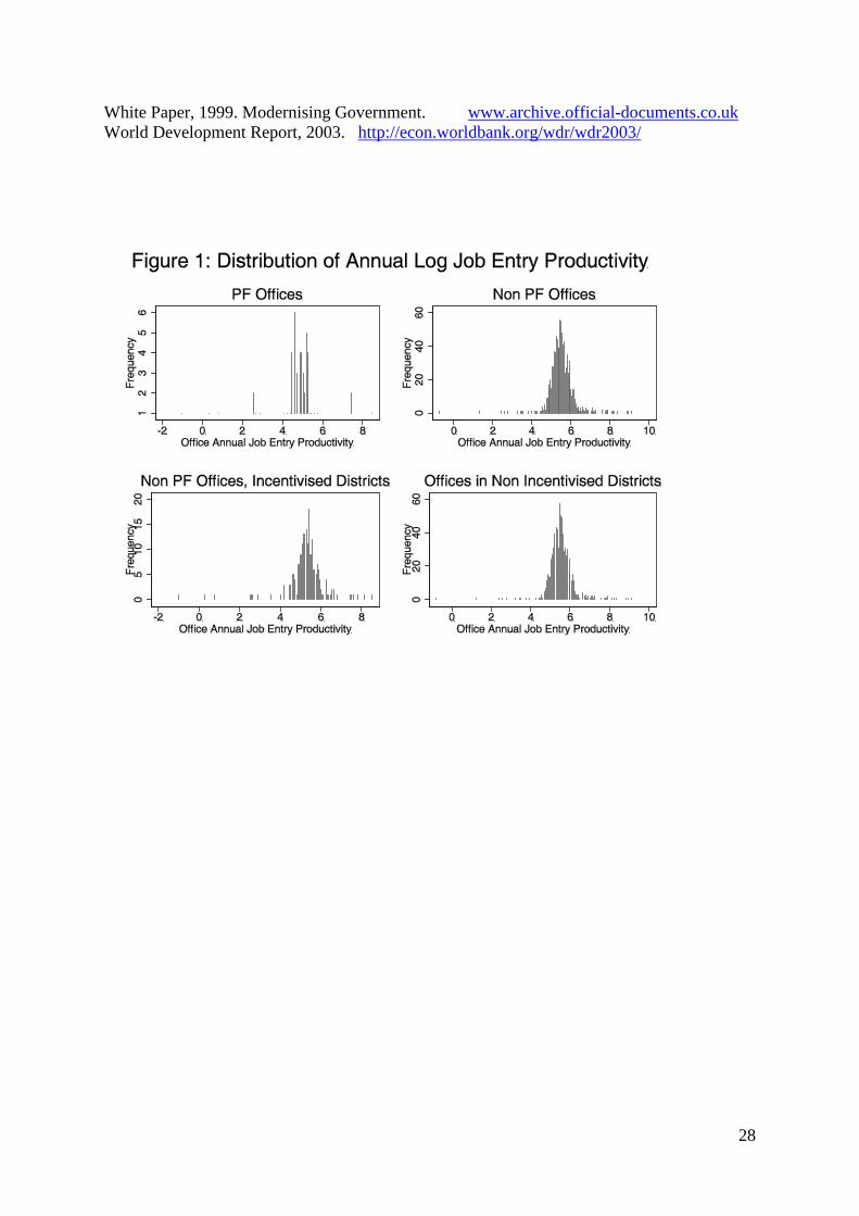
Figure 1 shows the distribution of the annual job entry productivity across different office and

district types. Comparing offices in non-incentivised districts with non-PF offices in

incentivised districts is closest to a like-with-like comparison and the distributions are fairly

similar. PF offices, on the other hand, are clearly associated with lower mean job entry

figures. We exclude PF offices from our main analysis but test for the robustness of this

choice in Section 3.4. We do include another kind of office that during the scheme also were

designated as pathfinder offices, Job Centre Plus Offices. These became pathfinder offices

late in the scheme, for example 82% in the final two months, hence little disruption was

expected. We again test the robustness of this choice.

The incentive scheme ran from April 2002 to March 2003, and this is the period of our data.

Note that although Jobcentre Plus employees were informed about the incentive scheme in

April 2002, they did not know the specific targets until June 2002. It would obviously be very

14

desirable to have data before the scheme was implemented to allow a difference-in-difference

technique. Unfortunately this is simply not possible as the district boundaries (that defined

the scheme) were re-drawn in 2002, and different PSA targets were in operation before April

2002, implying a different set of output measures.

2.2 Empirical Specification

We aim to answer three questions. First, is the productivity of public sector workers

influenced by financial incentives? Second, does free-riding matter in a team-based incentive

scheme? We sub-divide this into the free-riding deriving from many workers in an office, and

into that arising from many offices in a district. Third, does the differential measurement

precision of the different targets influence behaviour?

The outcomes we focus on are log job entry productivity as the quantity measure and the

quality of service to job seekers (denoted JSQ), the quality of service to firms (denoted EMQ)

and the business delivery target (denoted BDT) as the three quality measures.

The pilot scheme introduced the incentive structure in the 17 Pathfinder (PF) districts, leaving

73 districts as controls. So all offices in each PF district were incentivized as part of the

district team and no offices in the control districts were incentivized. This raises two issues

for identification: how districts were chosen as PF districts, and how we can distinguish

between the effects of the incentive scheme and the effects of the introduction of PF offices.

Identification of this model comes from random treatment of non-PF offices within PF

districts. Assignment to the pilot scheme was at district level and was based on a district

being designated a PF district (defined as a district containing at least one PF office). PF

offices were to be spread across all 11 Jobcentre Plus regions. The specific sites in each

region were chosen by Field Directors and their District Managers on the grounds that their

management would be able to cope well with the demands of the new structure. Clearly PF

status is likely to be correlated with other outcomes. But PF offices were located across the

regions, and the selected offices were to reflect a “cross-section of different communities and

customer bases, i.e. from large inner-city offices to those in smaller towns, suburbs and rural

areas.”18

18 Private communication.

The consequence of classification of an office to PF status was that all other offices

15

within this district became PF district. This suggests that assignment at district level to the

treatment category is stratified random. Assignment of offices other than the PF office itself

to the pilot is random. Those offices are in the pilot on grounds entirely unrelated to their own

performance and characteristics.19

The two mechanisms together imply that for offices other than the PF office itself,

assignment to the scheme is random and this is what we exploit here to give us identification

of the impact of the scheme. As selection of PF offices is not random, they are excluded from

all analysis. For the remaining offices, given random assignment, we can identify the

incentive scheme effect from regression analysis.

We estimate the quantity measures at office level:

ododdod βXISy νγα +++= (1)

where y is log total job entry productivity in office o in district d, X is a set of covariates and

ν is random noise. γ denotes the effect of incentivisation status (IS), our parameter of

interest. To test for the presence of free riding within teams of the incentive scheme we

interact IS with the number of workers within an office and the number of offices within a

district.

We estimate the quality measures at district level:

dddd uZISy +++∂= ηλ (2)

y={JSQ, EMQ, BDT}, λ denotes the effect of incentivisation and u the error term. To test for

free riding at the district level we interact IS with the number district staff and with the

number of offices at district level. The controls (Z) are aggregated to a district level. We

control additionally for the size of the districts through the total number of staff in the district

as, unlike the quantity equation, quality does not measure productivity but rather the level of

the outcome20

.

Our identification assumption for the office level analysis is

E(yod|ISd=1,PFod=0,Xod)=E(yod|ISd=0,Xod); E(vod|ISd,Xod,PFod

and is the same for district level analysis, with the office subscript omitted.

=0)=0

19 Offices are only linked together in districts through spatial proximity, not through performance levels, for example. In addition, we control for spatial factors such as the local labour market in influencing performance.

16

Table A2 shows that incentivised districts are larger, both with more staff per office (485

compared to 268 on average), and more offices (15 compared to 11). They appear to face

very similar labour market conditions. Incentivised offices have slightly more staff (32

compared to 27) but similar labour market tightness. To further ensure that our comparison of

incentivised offices with non-incentivised offices compares like-with-like we use Propensity

Score Matching to select our control offices.

We undertake the matching as follows. Even though districts are the basis for assignment into

the treated category, we compute propensity scores at office level because offices are the unit

of analysis. We include all non-PF offices in incentivised districts and all offices in non-

incentivised districts. We exclude PF offices from our analysis on the grounds they are

different from the other offices. This leaves 912 offices. We estimate the conditional

probability of assignment to incentivisation status based on a set of observable variables.

These variables might influence choice of pilot areas and/or the outcome variables.21

We

employ a nonparametric regression method with kernel weights proportional to an

Epanechnikov kernel and bootstrap to calculate the standard errors using 100 replications

with replacement. Common support is imposed on the match following Heckman, Ichimura

and Todd (1997). This excludes 71 treated offices.

3. Results

We present results first for the main quantity variable, testing to see whether the incentive

scheme had any effect on productivity and for evidence of free-riding. Next, the effect of the

scheme on quality measures is assessed, to examine whether the effect of the scheme changes

across outcomes measured with different precision. Finally, we estimate quantity and quality

jointly, allowing for production interdependencies.

3.1 Quantity – Job Entry Productivity

3.1.1 Descriptive Analysis

20 Quality measures were recorded as percentages, making it impossible to normalise by office size. 21 The propensity score estimator (probit) is shown in Table A4 and the quality of the matching in Table A5. The latter shows significant differences in the pre-matched sample for variables including the propensity score,

17

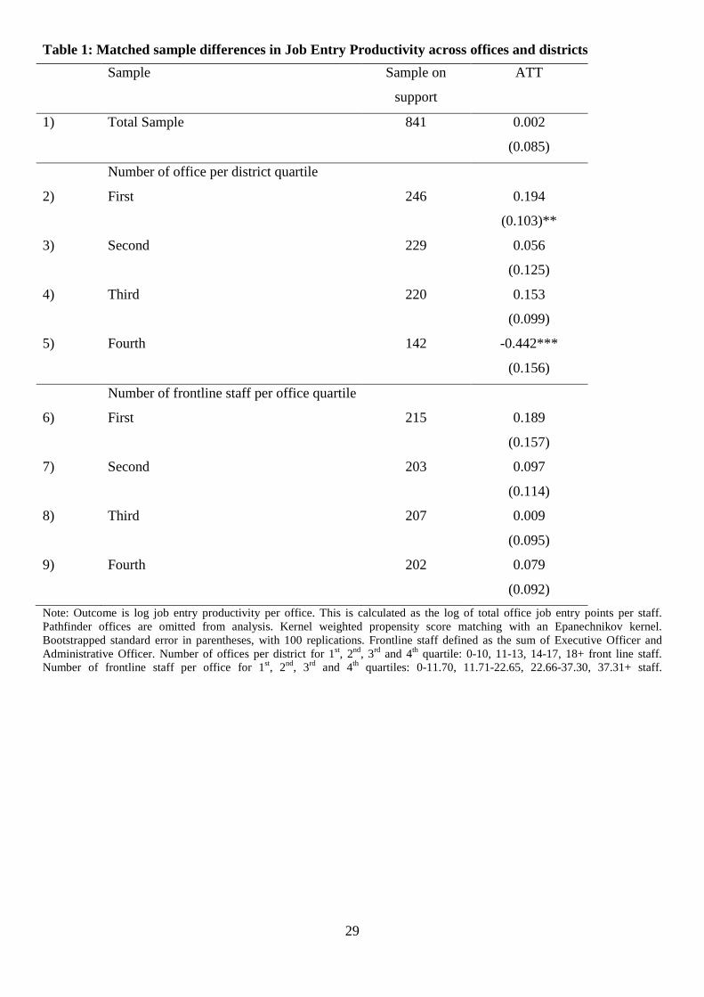
The first row of Table 1 shows a simple comparison of the mean job entry productivity

difference for the matched sample of treated and non-treated offices. The results indicate a

negligible and insignificant effect of the incentive scheme. Those offices subject to treatment

had slightly higher job entry productivity than non-treated offices. Specifically, the

coefficient 0.002 translates into an average treatment of the treated (ATT) of 0.67 job entry

points per person. This is a very small effect, equivalent to finding employment for less than

one employed individual.22

We look for evidence of heterogeneity in this effect linked to the free-rider/co-ordination

issues discussed above. In rows 2-5 and rows 6-9 of Table 1 we split the matched sample by

number of offices within the district (district size) and the staff per office (office size)

respectively. Small treated districts have significantly higher productivity than non-treated.

As district size increases, the effect of the incentive scheme on job entry productivity tends to

decline such that there is a significant and negative effect of the incentive scheme for districts

in the highest size quartile. This translates on average into 118 job entry points per person,

which is nearly 10 unemployed lone parents or 118 employed job searchers. The exception is

for districts in the third quartile, where there is a more positive effect than the second quartile,

but results are not statistically significant. Similarly, splitting the sample by quartile of office

size, the ATT declines across office quartile, although these estimates are insignificant.

Despite an insignificant total effect of the incentive scheme, these results are suggestive of

free riding both within and between offices and of coordination issues.23

The mean

productivity difference between treated and control districts (offices) declines in the district

(office) size. To explore this further, we move to a conditional regression analysis.

3.1.2 Regression Analysis

standard deviation of labour market conditions and number of offices per district. However post matching, there the significant difference was only an interaction between staff and offices per district. 22 See Table A3 for translation of client group categories into points 23 Note that we tested for interactions across both office and district size in the ATT. For example, the negative ATT in large districts may be strongest in large offices, or vice versa. Estimating the ATT for samples split by both the size of the office and the district shows that for large districts the ATT was more negative for office sizes above the median. For small districts, there was no evidence of an effect as office size changed. However, with such small sample sizes, no estimates were significant.

18

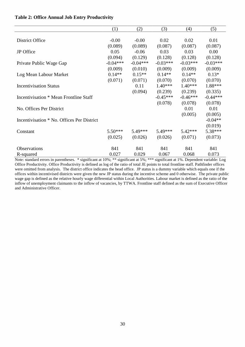
Table 2 presents the results for the log annual job entry productivity. This is for the sample in

Table 1: only offices producing job entries are included in the analysis, PF offices are

excluded and we include only offices on common support in the matching.

We present a number of different specifications for the effects of the incentive scheme along

with the office characteristics. We start with the effect of basic office characteristics in

column 1. District Offices (which have central administrative functions) are equally

productive as other offices. A Job Centre Plus office (one which became a PF office within

the year) has no different job entry productivity from other offices, whilst the gap between

wages in the private and public sector has a negative productivity effect as expected, as a

higher wage gap implies lower quality workers in the public sector. Finally, the state of

demand in the labour market has a positive and significant influence on job entry

productivity.24

Similar to the propensity score matching descriptives, column 2 shows an insignificant

treatment effect on average. In an incentive scheme where performance is measured at a team

level, the marginal return to individual effort decreases in the team size, which raises the

incentive to free ride. Column 3 tests for the presence of free riding within offices, including

an interaction between treatment status and the office size. Column 4 adds the number of

offices per district effect. Column 5 explores free riding across offices by adding an

interaction between treatment status and the number of offices per district to this

specification.

Allowing for heterogeneity in the effect by the team size in columns 3-5 shows a large

positive mean incentive effect, equivalent to 467 job entry points per staff member. But this

positive treatment effect falls significantly with both the office size (column 3) and district

size (column 5), . Increasing office size by one frontline worker and increasing district size

by one office lowers job entry productivity by 5 and 18 job entry points, respectively. Thus

the average incentivisation effect of zero masks a positive mean effect in small offices and

small districts and a negative effect in large offices and large districts.

24 Note that in an earlier version of the paper, we conducted a 2-stage approach, firstly calculating an office fixed effect and subsequently regressing office characteristics on this. The time-series variation and cross-

19

Our finding of a negative impact of office and district size is consistent with the discussion

above that bigger offices and offices in bigger districts face a greater free riding and

coordination problem. This echoes Gaynor et al. (2004) but is inconsistent for example, with

Knez & Simester (2001). Knez and Simester argue that peer monitoring worked in

Continental because employees worked in relatively small autonomous groups, within which

monitoring and enforcement of group norms were sustainable. In our setting the sub-teams

were offices, some of which had over 200 staff members. The consequence of this was that

the free riding effect dominated.

3.2 Quality – Job-Seeker, Employer Service and Business Delivery

We adopt a similar approach to modelling quality outcomes. We model the quality of service

to job-seekers JSQ and to employers EMQ and a measure of quality of business service,

BDT. These outcomes are only measured quarterly and at district level, compared to the

quantity analysis at a monthly office level. This has implications for behaviour as set out

above, but also for our estimation, reducing sample size from around 900 offices to just 90

districts.

Table A1 gives the (log) mean response on these three quality measures, which translate into

an 88.2% success rating for EMQ, 84.3% for JSQ and 96.3% for BDT. The table also shows

little variation in these scores across districts for JSQ and BDT, but more for EMQ. All

districts hit their targets for JSQ, whilst only 64% and 51% did for EMQ and BDT,

respectively.

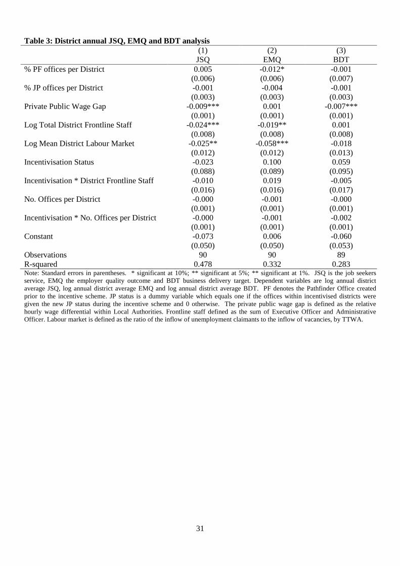
Table 3 shows the results for the district annual averages for JSQ, EMQ and BDT. Few

variables are estimated to have a significant effect, due in part to the small number of

observations and a lack of variation in the outcomes and in the case of JSQ the targets

possibly having been set too low. For JSQ and EMQ, the number of staff in the office has a

negative effect. This may arise from a more personal service in smaller offices. The tightness

of the labour market has a negative impact, the magnitude of which is largest for EMQ. This

is intuitive, as a tight labour market means a difficult time for employers to fill vacancies.

There is no significant impact of any term involving incentivisation status on either of the

three quality outcomes.

section variation work in the opposite direction, thereby cancelling out the total labour market effect seen in

20

The lack of significant effect of incentivisation on quality outcomes can be taken in two

different ways. First, it could be argued that the scheme failed to elicit any increase. This is

not surprising in that the precision of the monitoring technology for quality was low,

measured infrequently at a high level of aggregation. This implied a lower marginal return to

effort and consequently low optimal effort allocation to this component of the job. Second, it

could be viewed more positively as showing that despite the greater effort on quantity,

quality did not actually fall, a standard failing of many incentive schemes. Whether this is

due to the incentive scheme explicitly targeting quality, or whether due to the existence of

sufficient slack to permit the increase in quantity, is difficult to say.

3.3 Quantity and Quality Together

The contrast between the significant effect of the scheme on quantity and lack of effect on

quality is interesting. It may be that this arose from the differing measurement precision for

the three aspects of the job, or it may simply be statistical – 90 observations in one case

compared to over 900 in the other. Since this matters for incentive scheme design, we get at

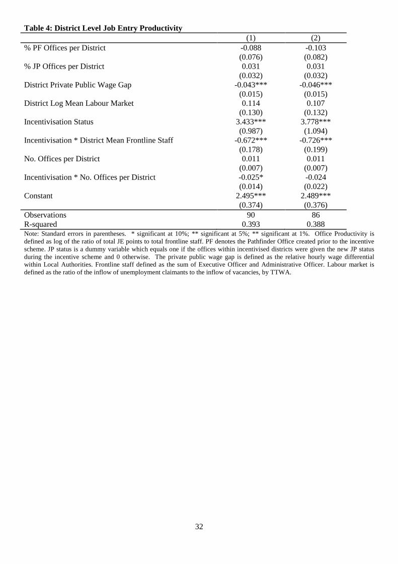
this by re-running the quantity regression at district level. To do this, we used as the

dependent variable log district annual job entry productivity. The results are in Table 4. We

run two samples to calculate the productivity effect. In column 1 we use the full sample as

used in the quality analyses of Table 3 and in column 2 we use the common support sample

used in the quantity analyses of Table 2.

Table 4 shows that for both samples there is a positive impact of incentivisation, which

declines with office and district size, although the latter interaction is significant only for the

full sample of 90 districts. This suggests that the differences between Tables 2 and 3 are not

due to size of the sample, but there is something different about the behavioural response to

the quantity and quality targets. This could be explicable in terms of the differences in the

precision of the monitoring technology. This arises in part from the differences in the nature

of quantity and quality measurement (one is based on easily countable job placements at

monthly intervals, the other on the views from surveys at quarterly intervals) and in part from

the much greater degree of aggregation of the quality measure used in the incentive scheme

(district compared to office for the quantity measure).

Table 2.

21

It could be argued that since time allocated to quantity or to quality is determined jointly, we

need to take account of that in estimation. The first step is simply to establish whether good

performance on one dimension is positively or negatively correlated with good performance

on the other. In fact, there is little correlation between quantity and quality and a positive

correlation between quality measures except EMQ and BDT25. If we take EMQ as more

useful a measure given the low variation in JSQ and BDT, there is a very low association26

.

Therefore we do not think that the results arise because time spent on quantity reduces the

amount of time to achieve quality, but instead arises because of differences in measurement

precision which means that output is much less related to individual productivity. These

findings also have support from Gaynor and Pauly (1990) who showed that output was

significantly higher in medical practices in which compensation was more directly related to

productivity.

3.4 Robustness tests

We examine whether the results of the treatment effect on job entry productivity from column

5 of Table 2 are sensitive to various specification choices in the main regression analysis.

These are presented in Table 5. In column 1 the dependent variable is changed to log job

entry productivity, standardised so that the coefficients represent standard deviations in

productivity and column 2 changes the dependent variable to be the level of standardised

productivity. In both cases, while the magnitudes of the coefficients change, the positive

incentive effect remains and is decreasing in office size. It is also decreasing in district size,

though this interaction is no longer significant. In column 3, we move away from an analysis

of the productivity effects and instead regress on the log job entry points per office,

controlling for office level frontline staff as a regressor. We find again a positive treatment

effect, declining in team size, and while the interaction between treatment status and office

size is no longer significant the interaction with district size is.

Table 2 excluded PF offices from the analysis and included the JP offices as these tended to

be introduced quite late in the incentive scheme. In column 4 and 5 of Table 5 we include the

PF offices and exclude the JP offices respectively. Our results prove robust to both of these

25 The correlation of average annual job entry productivity with JSQ, EMQ and BDT is 0.20, 0.13 and 0.24, between JSQ and EMQ and BDT is 0.38 and 0.49 and between EMQ and BDT is -0.041.

22

changes and both sets of interactions and the main effects are significant. In summary, the

quantity effects are broadly robust to various specification change.

4. Valuing the impact of the incentive scheme

The mean effect of the scheme is zero. So across all offices in the scheme there were no

gains. However, our estimates show that for small offices and small districts there were

increases in quantity following the scheme. In this section, we ask the question if there

scheme were to be introduced in the appropriate settings i.e. in small offices and districts,

what value might it have?

We can evaluate the quantitative importance of the change in the quantity outcome in three

ways. First we compare the number of people placed into jobs with the monetary cost of the

scheme, thereby calculating the cost per placement. Second, we estimate the decrease in the

unemployment rate and third we compare the benefits of the incentive scheme to a general

pay rise in the government agency.

4.1 The cost per placement

Given the estimates in Table 2, column 5, we can straightforwardly calculate the distribution

of change in job entry productivity associated with the incentive scheme. The fitted value

from the regression is calculated using only variables related to treatment (the treatment

effect itself plus any interactions), translated into job entry points then converted into a

proportion of total job entry points for the treated office. Since the impact varies according

to office and district size, we report this percentage change across the distribution as well as

the mean in Table 6. As would be expected from Table 2 column 2, the overall effect of

incentivisation is small and negative, at nearly -1%. There is a substantial positive effect in

small offices in small districts and this effect falls across both dimensions of office and

district size.

The mean percentage increases in small offices (in any district) and the mean in small

districts (across all offices) are 39% and 25% respectively. A 39% and 25% change in job

entry productivity translates to 6,000 and 2,030 job entry points respectively, or

26 We also estimate the district level annual quantity and EMQ models jointly using SUR, but as we would

23

approximately 1,200 and 400 extra people. The ex post cost of the job entry component of the

scheme was around £272,100, 0.21% of the salary bill for the 17 incentivised districts. We

estimate this from the payments made for 5 of the 17 districts hitting their job entry target and

earning 1% of salary (allowing for different numbers of staff). All 5 who hit were small

districts. Consequently, in the best case scenario of targeting the incentive scheme towards

small districts, the scheme cost £226.75 per job placement.

4.2 Impact of Scheme on Unemployment

It is clear that the operation of the incentive scheme does not create new jobs. Nor does it

help into employment people who would otherwise have remained unemployed forever. So a

‘cost per job created’ is not directly appropriate. Rather, the scheme accelerates movement

into work of its clients. Given an unemployment exit rate of x, and an inflow rate of i, the

steady-state unemployment rate is given by ( )xiiu +=* . We assume that the inflow rate is

unaffected by the JP incentive scheme, and that the exit rate is x = k. (JE/U), where k > 1

allows that not all those leaving unemployment do so to jobs and U is the stock of

unemployed. Translating the production function in equation (1) into levels,

JEod=αVodγUod

δWodexp(vod), where V and W denote vacancies and office characteristics

respectively. This gives x = k.A.(V/U)1-α

( ) ( )*, 1* uixxu −−=+−=

αη

, and A = α.W , is the JP office effect, with α (office

effort) depending on the incentive scheme. It is easy to show that:

(9)

where η denotes elasticity. Again, taking the mean value of a 25% increase from the small

districts and 39% from small offices, this produces a mean percentage decrease in

unemployment of 23.75% and 37.05% respectively. Given a national mean unemployment

rate of 5.1% at the end of 2002, this is a very large fall of 1.2 and 1.9 percentage points.

4.3 Incentive Scheme, a General Pay Rise or More Staff

A final metric for evaluating the size of the incentivisation effect is to compare it to raising

the quality of staff through a general pay rise. We can do this straightforwardly through the

estimated production function. Using column 5 of table 2, we compute the change in the

private-public pay differential (£ per hour) required to produce a 25% and 39% increase in

job entry productivity. This is given by ln(1.25)/(-0.03), equal to –7.44 and -10.98. Thus a

£7.44 and £10.95 an hour pay increase in the public sector would, through recruitment of

expect from the low correlation found above, there is only a small change in the standard errors.

24

higher quality staff, on average elicit the same output improvement as this scheme does in

small districts and small offices respectively. Given that the average hourly pay in the

organisation was £8.70 at the time, a £7.75 or £10.95 per hour increase would be extremely

expensive, and way above the cost of the incentive scheme.

In conclusion had the scheme been applied only in small offices and small districts, it would

have been costs effective. Even a 1% increase in output would have made this scheme cost

effective on the basis of the estimated parameters.

5. Conclusions

There is a lack of robust evidence on the role and impact of performance pay in the public

sector, even though this is a sector that employs as many people in the UK and US as

manufacturing does. This paper starts to fill that gap by providing an evaluation of a pilot

scheme of financial incentives in a major UK government agency, Jobcentre Plus. The

incentive scheme was based on team performance rather than individual and covered five

different targets, measured with varying degrees of precision. We focus on three main issues:

whether performance pay matters for public service workers, what the team basis of the

scheme implies, and the impact of the differential measurement precision.

We show that the use of performance pay had no effect on the main quantity measure (job

placement productivity) at the mean, but that there was important heterogeneity of response.

The heterogeneity was patterned as one might expect from a free rider versus peer monitoring

perspective. We found that the incentives had a substantial positive effect in small offices

and in offices in small districts. In districts with many offices and in large offices, there was a

negative effect. Our interpretation of this is that peer monitoring and better information

flows can overcome free rider problems in small units, but that it fails in teams made up of

many people, or dispersed across many offices.

The impact of performance pay on quantity was not matched by any impact on different

quality measures. One key difference between the quantity and quality targets is the precision

of measurement. Quantity in this scheme was measured monthly at office level, with a clear,

direct effect of an individual’s effort to the target measure. Quality measures were based on

25

samples of different clients’ experiences, and were only measured quarterly at district level.

In this case, an individual’s effort is only measured probabilistically, and is in any case

submerged in a much broader total. Our interpretation of this finding is that individuals

responded to this by focussing their effort on quantity rather than quality (see Gaynor and

Pauly, 1990).

Could such a scheme be cost effective? Given the heterogeneity of response the overall mean

impact is close to zero. But if we examine the size of the positive effect in the small districts

where the scheme did work our estimates suggest that if the scheme was well targeted, the

use of incentive pay could deliver equivalent output increases to a rise in the quality of

recruited staff through a pay rise, at very significantly lower cost. Given that the scheme was

not particularly high powered (in contrast, for example, to Kahn et al. 2001), this suggests

that incentive schemes – if properly designed – can be useful in the public sector as a means

of increasing output without needing very large incentive payments.

There are a number of caveats. First, the scheme only operated for one year, and so the results

may include a “first year” novelty effect in addition to the pure incentive effect. Furthermore,

if a ‘ratchet’ design of continual percentage improvements were repeated in a dynamic

setting, the optimal response would be different to the response we have measured to a

possibly once-only pilot. Second, the outcome could be the result of performance

management per se, rather than the financial reward attached. But this is unlikely in that the

same performance management system was in place everywhere, across the control offices as

well as the pilot offices. It may be that the financial incentives led managers to take the

existing framework more seriously but that is surely part of the aim of performance pay.

Third, Jobcentre Plus may have been an organisation with a lot of slack in it. Unemployment

and job-seeking had fallen considerably since the peaks of the 1980s up to the start of the

scheme, and it may be that staff were less hard-pressed than before. Finally, it may be that the

assignment to the pilot was not completely random and differentially included high-

performing offices. Whilst possible, this seems to be unlikely given the nature of the

assignment process. Districts were included in the pilot if one office in that district had been

selected to be a PF office. Given the few operational links between offices, this is essentially

random assignment for other offices in that district.

26

We finally draw some tentative conclusions for the design of team level performance pay

schemes in the public sector. There are some obvious conclusions – team size needs to be

small and preferably not dispersed over many sites. The connection between effort and output

needs to be as clear and well-measured as possible. There are trade-offs here: precise

measurement may be very expensive if conducted for many small teams. Finally, there are

lessons for the structure of organisations as well as for the nature of optimal incentive

schemes. Dewatripont, Jewitt and Tirole (1999) make this point in the context of mission

definition, but it also applies here to team size and task measurement. If incentives are indeed

a very cost-effective way of inducing greater output given the right team size, then

organisations could be re-structured to create natural teams of the appropriate size. Such re-

structuring could also allow for relative performance evaluation to filter away common

uncertainty. These points also fit well with the general ethos of devolved agency inherent in

many current public service reforms.

References Baiker, K., Jacobson, M., 2007. Finders keepers: forfeiture laws, policing incentives, and

local budgets. Journal of Public Economics 91, 2113-2136. Baker, G., 2002. Distortion and risk in optimal incentive contracts. Journal of Human

Resources 37(3), 728-751. Bandiera, O., Guiso, L., Prat, A., Sadun, R., 2011. Matching firms, managers and incentives.

NBER Working Paper 16691. Barnow, B. A., 2000. Exploring the relationship between performance management and

program impact: A case study of the JTPA. Journal of Policy Analysis and Management 19(1), 118-141.

Besley, T., Ghatak, M., 2003. Incentives, choice and accountability in the provision of public services. Oxford Review of Economic Policy 19(2), 235 – 249.

Besley, T., Ghatak, M., 2005. Competition and incentives with motivated agents. American Economic Review 95(3), 616-636.

Bhattacherjee, D., 2005. The effects of group incentives in an Indian firm: evidence from payroll data. Review of Labour Economics and Industrial Relations 19(1), 147-173.

Bloom, N., Van Reenen, J., 2010. Human resource management and productivity. NBER Working Paper 16019 and forthcoming. In: Ashenfelter, O and Card, D. Handbook of Labor Economics 4.

Burgess, S., Propper, C., Ratto, M.L., von Hinke Kessler Scholder, S., Tominey, E., 2010. Smarter task assignment or greater effort: what makes a difference in team performance? The Economic Journal 120(547), 968-989.

Burgess, S., Ratto, M.L., 2003. The role of incentives in the public sector: issues and evidence. Oxford Review of Economic Policy 19(2).

Dewatripont, M., Jewitt, I., Tirole, J., 1999. The economics of career concerns, Part II: Application to missions and accountability of government agencies. The Review of Economic Studies 66(1), 199-217.

27

Dixit, A., 2002. Incentives and organisations in the public sector: an interpretative review. Journal of Human Resources 37(4), 696-727.

Francois, P., 2000. ‘Public service motivation’ as an argument for government provision. Journal of Public Economics 78, 275-299.

Gaynor, M., Pauly, M., 1990. Compensation and productive efficiency in partnerships: evidence from medical group practice. Journal of Political Economy 98(33), 544-573.

Gaynor, M., Rebitzer, J.B., Taylor, L.J., 2004. Physician incentives in health maintenance organizations. Journal of Political Economy 112(4), 915-931.

Gravelle, H., Sutton, M., Ma, A., 2010. Doctor behaviour under a pay for performance contract: treating, cheating and case finding? The Economic Journal

Hamilton, B.H., Nickerson, J.A., Owan, H., 2003. Team incentives and worker heterogeneity: an empirical analysis of the impact of teams on productivity and participation. Journal of Political Economy 111(3), 465-497.

120, 129-156.

Heckman, J., Ichimura, H., Todd, P., 1997. Matching as an econometric evaluation estimator: evidence from evaluating a job training programme. Review of Economic Studies 64, 605-654.

Heckman, J., Smith, J., Taber, C., 1996. What do bureaucrats do? The effects of performance standards and bureaucratic preferences on acceptance into the JTPA program. In: G. Libecap. (Eds.). Advances in the study of entrepreneurship, innovation and growth. 7. Greenwich, CT: HAI Press, 191-217.

Holmström, B., 1982. Moral hazard in teams. Bell Journal of Economics 13, 324-340. Kahn, C.M., Silva, E.C.D., Ziliak, J.P., 2001. Performance-based wages in tax collection: The

Brazilian tax collection reform and its effects. Economic Journal 111(468), 188-205. Kandel, E., Lazear, E., 1992. Peer pressure and partnerships. Journal of Political Economy

100(4), 801-817. Knez, M., Simester, D., 2001. Firm-wide incentives and mutual monitoring at Continental

Airlines. Journal of Labor Economics 19(4), 743-772. Lavy, V., 2009. Performance pay and teachers’ effort, productivity, and grading ethics.

American Economic Review 99(5), 1979-2011. Lazear, E., 2001. Performance pay and productivity. American Economic Review 90(5),

1346-1361. Makinson, J., 2000. Incentives for change. Rewarding performance in national government

networks. Public Service Productivity Panel. HMSO. Mullen, K., Frank, R., Rosenthal, M., 2010. Can you get what you pay for? Pay-for-

performance and the quality of healthcare providers. The RAND Journal of Economics 41(1), 64-91.

Nickell, S., Quintini, G., 2002. The consequences of the decline in public sector pay in Britain: a little bit of evidence. Economic Journal 112(477), 107-118.

Osborne, D., Gaebler, T., 1993. Reinventing government: how the entrepreneurial spirit is transforming the public sector. New York: Plume Books, (Penguin Group).

Paarsch, H., Shearer, B., 2000. Piece rates, fixed wages, and incentive effects: statistical evidence from payroll records. International Economic Review 41(1), 59-92.

Prendergast, C., 1999. The provision of incentives in firms. Journal of Economic Literature 37, 7-63.

Prendergast, C., 2002. The tenuous trade-off between risk and incentives. Journal of Political Economy 110(5), 1071-1102.

Propper, C., Van Reenen, J., 2010. Can pay regulation kill? Journal of Political Economy 118(2), 222-273

Ratto, M., Tominey, E., Vergé, T., 2010. Rewarding collective performance to induce cooperation. Mimeo University of Bristol.

28

White Paper, 1999. Modernising Government. www.archive.official-documents.co.uk World Development Report, 2003. http://econ.worldbank.org/wdr/wdr2003/

29

Table 1: Matched sample differences in Job Entry Productivity across offices and districts Sample Sample on

support

ATT

1) Total Sample 841 0.002

(0.085)

Number of office per district quartile

2) First 246 0.194

(0.103)**

3) Second 229 0.056

(0.125)

4) Third 220 0.153

(0.099)

5) Fourth 142 -0.442***

(0.156)

Number of frontline staff per office quartile

6) First 215 0.189

(0.157)

7) Second 203 0.097

(0.114)

8) Third 207 0.009

(0.095)

9) Fourth 202 0.079

(0.092) Note: Outcome is log job entry productivity per office. This is calculated as the log of total office job entry points per staff. Pathfinder offices are omitted from analysis. Kernel weighted propensity score matching with an Epanechnikov kernel. Bootstrapped standard error in parentheses, with 100 replications. Frontline staff defined as the sum of Executive Officer and Administrative Officer. Number of offices per district for 1st, 2nd, 3rd and 4th quartile: 0-10, 11-13, 14-17, 18+ front line staff. Number of frontline staff per office for 1st, 2nd, 3rd and 4th quartiles: 0-11.70, 11.71-22.65, 22.66-37.30, 37.31+ staff.

30

Table 2: Office Annual Job Entry Productivity (1) (2) (3) (4) (5) District Office -0.00 -0.00 0.02 0.02 0.01 (0.089) (0.089) (0.087) (0.087) (0.087) JP Office 0.05 -0.06 0.03 0.03 0.00 (0.094) (0.129) (0.128) (0.128) (0.128) Private Public Wage Gap -0.04*** -0.04*** -0.03*** -0.03*** -0.03*** (0.009) (0.010) (0.009) (0.009) (0.009) Log Mean Labour Market 0.14** 0.15** 0.14** 0.14** 0.13* (0.071) (0.071) (0.070) (0.070) (0.070) Incentivisation Status 0.11 1.40*** 1.40*** 1.88*** (0.094) (0.239) (0.239) (0.335) Incentivisation * Mean Frontline Staff -0.45*** -0.46*** -0.44*** (0.078) (0.078) (0.078) No. Offices Per District 0.01 0.01 (0.005) (0.005) Incentivisation * No. Offices Per District -0.04** (0.019) Constant 5.50*** 5.49*** 5.49*** 5.42*** 5.38*** (0.025) (0.026) (0.026) (0.071) (0.073) Observations 841 841 841 841 841 R-squared 0.027 0.029 0.067 0.068 0.073

Note: standard errors in parentheses. * significant at 10%; ** significant at 5%; *** significant at 1%. Dependent variable: Log Office Productivity. Office Productivity is defined as log of the ratio of total JE points to total frontline staff. Pathfinder offices were omitted from analysis. The district office indicates the head office. JP status is a dummy variable which equals one if the offices within incentivised districts were given the new JP status during the incentive scheme and 0 otherwise. The private public wage gap is defined as the relative hourly wage differential within Local Authorities. Labour market is defined as the ratio of the inflow of unemployment claimants to the inflow of vacancies, by TTWA. Frontline staff defined as the sum of Executive Officer and Administrative Officer.

31

Table 3: District annual JSQ, EMQ and BDT analysis (1) (2) (3) JSQ EMQ BDT % PF offices per District 0.005 -0.012* -0.001 (0.006) (0.006) (0.007) % JP offices per District -0.001 -0.004 -0.001 (0.003) (0.003) (0.003) Private Public Wage Gap -0.009*** 0.001 -0.007*** (0.001) (0.001) (0.001) Log Total District Frontline Staff -0.024*** -0.019** 0.001 (0.008) (0.008) (0.008) Log Mean District Labour Market -0.025** -0.058*** -0.018 (0.012) (0.012) (0.013) Incentivisation Status -0.023 0.100 0.059 (0.088) (0.089) (0.095) Incentivisation * District Frontline Staff -0.010 0.019 -0.005 (0.016) (0.016) (0.017) No. Offices per District -0.000 -0.001 -0.000 (0.001) (0.001) (0.001) Incentivisation * No. Offices per District -0.000 -0.001 -0.002 (0.001) (0.001) (0.001) Constant -0.073 0.006 -0.060 (0.050) (0.050) (0.053) Observations 90 90 89 R-squared 0.478 0.332 0.283 Note: Standard errors in parentheses. * significant at 10%; ** significant at 5%; ** significant at 1%. JSQ is the job seekers service, EMQ the employer quality outcome and BDT business delivery target. Dependent variables are log annual district average JSQ, log annual district average EMQ and log annual district average BDT. PF denotes the Pathfinder Office created prior to the incentive scheme. JP status is a dummy variable which equals one if the offices within incentivised districts were given the new JP status during the incentive scheme and 0 otherwise. The private public wage gap is defined as the relative hourly wage differential within Local Authorities. Frontline staff defined as the sum of Executive Officer and Administrative Officer. Labour market is defined as the ratio of the inflow of unemployment claimants to the inflow of vacancies, by TTWA.

32

Table 4: District Level Job Entry Productivity (1) (2) % PF Offices per District -0.088 -0.103 (0.076) (0.082) % JP Offices per District 0.031 0.031 (0.032) (0.032) District Private Public Wage Gap -0.043*** -0.046*** (0.015) (0.015) District Log Mean Labour Market 0.114 0.107 (0.130) (0.132) Incentivisation Status 3.433*** 3.778*** (0.987) (1.094) Incentivisation * District Mean Frontline Staff -0.672*** -0.726*** (0.178) (0.199) No. Offices per District 0.011 0.011 (0.007) (0.007) Incentivisation * No. Offices per District -0.025* -0.024 (0.014) (0.022) Constant 2.495*** 2.489*** (0.374) (0.376) Observations 90 86 R-squared 0.393 0.388 Note: Standard errors in parentheses. * significant at 10%; ** significant at 5%; ** significant at 1%. Office Productivity is defined as log of the ratio of total JE points to total frontline staff. PF denotes the Pathfinder Office created prior to the incentive scheme. JP status is a dummy variable which equals one if the offices within incentivised districts were given the new JP status during the incentive scheme and 0 otherwise. The private public wage gap is defined as the relative hourly wage differential within Local Authorities. Frontline staff defined as the sum of Executive Officer and Administrative Officer. Labour market is defined as the ratio of the inflow of unemployment claimants to the inflow of vacancies, by TTWA.

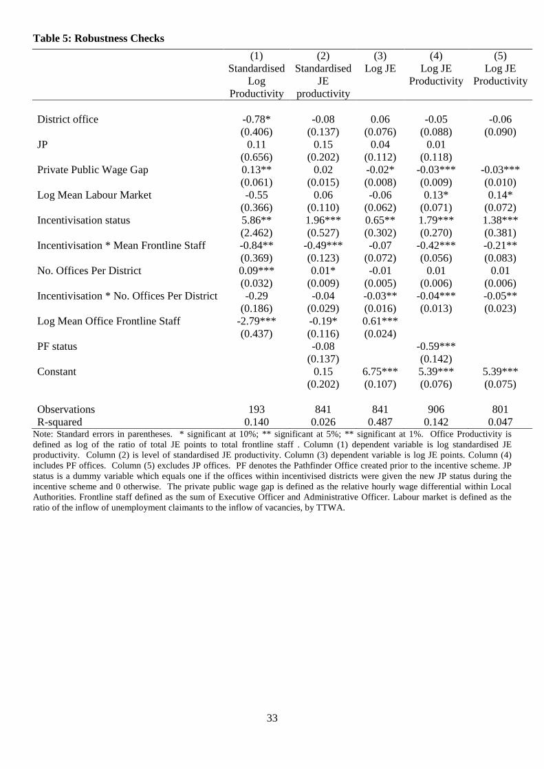
33

Table 5: Robustness Checks (1) (2) (3) (4) (5)

Standardised Log

Productivity

Standardised JE

productivity

Log JE

Log JE Productivity

Log JE Productivity

District office -0.78* -0.08 0.06 -0.05 -0.06 (0.406) (0.137) (0.076) (0.088) (0.090) JP 0.11 0.15 0.04 0.01 (0.656) (0.202) (0.112) (0.118) Private Public Wage Gap 0.13** 0.02 -0.02* -0.03*** -0.03*** (0.061) (0.015) (0.008) (0.009) (0.010) Log Mean Labour Market -0.55 0.06 -0.06 0.13* 0.14* (0.366) (0.110) (0.062) (0.071) (0.072) Incentivisation status 5.86** 1.96*** 0.65** 1.79*** 1.38*** (2.462) (0.527) (0.302) (0.270) (0.381) Incentivisation * Mean Frontline Staff -0.84** -0.49*** -0.07 -0.42*** -0.21** (0.369) (0.123) (0.072) (0.056) (0.083) No. Offices Per District 0.09*** 0.01* -0.01 0.01 0.01 (0.032) (0.009) (0.005) (0.006) (0.006) Incentivisation * No. Offices Per District -0.29 -0.04 -0.03** -0.04*** -0.05** (0.186) (0.029) (0.016) (0.013) (0.023) Log Mean Office Frontline Staff -2.79*** -0.19* 0.61*** (0.437) (0.116) (0.024) PF status -0.08 -0.59*** (0.137) (0.142) Constant 0.15 6.75*** 5.39*** 5.39*** (0.202) (0.107) (0.076) (0.075) Observations 193 841 841 906 801 R-squared 0.140 0.026 0.487 0.142 0.047

Note: Standard errors in parentheses. * significant at 10%; ** significant at 5%; ** significant at 1%. Office Productivity is defined as log of the ratio of total JE points to total frontline staff . Column (1) dependent variable is log standardised JE productivity. Column (2) is level of standardised JE productivity. Column (3) dependent variable is log JE points. Column (4) includes PF offices. Column (5) excludes JP offices. PF denotes the Pathfinder Office created prior to the incentive scheme. JP status is a dummy variable which equals one if the offices within incentivised districts were given the new JP status during the incentive scheme and 0 otherwise. The private public wage gap is defined as the relative hourly wage differential within Local Authorities. Frontline staff defined as the sum of Executive Officer and Administrative Officer. Labour market is defined as the ratio of the inflow of unemployment claimants to the inflow of vacancies, by TTWA.

34

Table 6: Mean Incentivisation Effect Number of frontline staff per office quartiles

First Second Third Fourth Mean

Number of

office per

Small districts: below median 64.63 34.18 12.50 -0.83 25.42

district Large districts: above median 27.11 -8.37 -23.81 -33.03 -10.32

Mean 39.01 -2.57 -14.30 -22.07 -0.87 Note: The incentivisation effect for incentivised offices was calculated using the fitted value from Table 2, column 5, using the variables incentivisation status and an interaction of this with office size and district size.

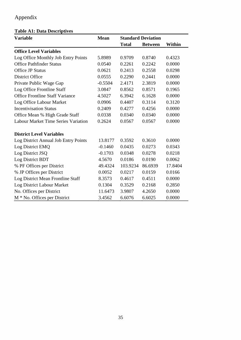
35

Appendix Table A1: Data Descriptives Variable Mean Standard Deviation Total Between Within Office Level Variables Log Office Monthly Job Entry Points 5.8989 0.9709 0.8740 0.4323 Office Pathfinder Status 0.0540 0.2261 0.2242 0.0000 Office JP Status 0.0621 0.2413 0.2558 0.0298 District Office 0.0555 0.2290 0.2441 0.0000 Private Public Wage Gap -0.5504 2.4171 2.3819 0.0000 Log Office Frontline Staff 3.0847 0.8562 0.8571 0.1965 Office Frontline Staff Variance 4.5027 6.3942 6.1628 0.0000 Log Office Labour Market 0.0906 0.4407 0.3114 0.3120 Incentivisation Status 0.2409 0.4277 0.4256 0.0000 Office Mean % High Grade Staff 0.0338 0.0340 0.0340 0.0000 Labour Market Time Series Variation 0.2624 0.0567 0.0567 0.0000 District Level Variables Log District Annual Job Entry Points 13.8177 0.3592 0.3610 0.0000 Log District EMQ -0.1460 0.0435 0.0273 0.0343 Log District JSQ -0.1703 0.0348 0.0278 0.0218 Log District BDT 4.5670 0.0186 0.0190 0.0062 % PF Offices per District 49.4324 103.9234 86.6939 17.8404 % JP Offices per District 0.0052 0.0217 0.0159 0.0166 Log District Mean Frontline Staff 8.3573 0.4617 0.4511 0.0000 Log District Labour Market 0.1304 0.3529 0.2168 0.2850 No. Offices per District 11.6473 3.9807 4.2650 0.0000 M * No. Offices per District 3.4562 6.6076 6.6025 0.0000

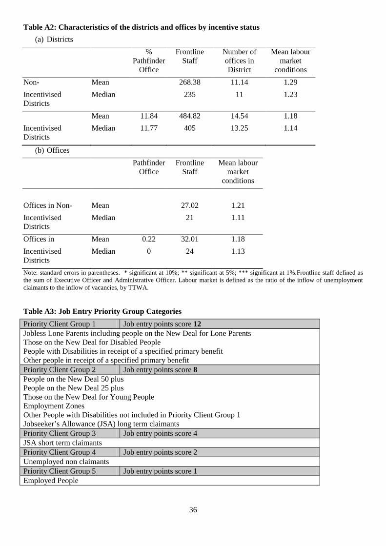
36

Table A2: Characteristics of the districts and offices by incentive status (a) Districts

% Pathfinder

Office

Frontline Staff

Number of offices in District

Mean labour market

conditions Non- Mean 268.38 11.14 1.29 Incentivised Districts

Median 235 11 1.23

Mean 11.84 484.82 14.54 1.18 Incentivised Districts

Median 11.77 405 13.25 1.14

(b) Offices Pathfinder

Office Frontline

Staff Mean labour

market conditions

Offices in Non- Mean 27.02 1.21 Incentivised Districts

Median 21 1.11

Offices in Mean 0.22 32.01 1.18 Incentivised Districts

Median 0 24 1.13

Note: standard errors in parentheses. * significant at 10%; ** significant at 5%; *** significant at 1%.Frontline staff defined as the sum of Executive Officer and Administrative Officer. Labour market is defined as the ratio of the inflow of unemployment claimants to the inflow of vacancies, by TTWA.

Table A3: Job Entry Priority Group Categories Priority Client Group 1 Job entry points score 12 Jobless Lone Parents including people on the New Deal for Lone Parents Those on the New Deal for Disabled People People with Disabilities in receipt of a specified primary benefit Other people in receipt of a specified primary benefit Priority Client Group 2 Job entry points score 8 People on the New Deal 50 plus People on the New Deal 25 plus Those on the New Deal for Young People Employment Zones Other People with Disabilities not included in Priority Client Group 1 Jobseeker’s Allowance (JSA) long term claimants Priority Client Group 3 Job entry points score 4 JSA short term claimants Priority Client Group 4 Job entry points score 2 Unemployed non claimants Priority Client Group 5 Job entry points score 1 Employed People

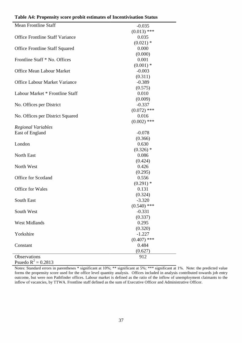
37

Table A4: Propensity score probit estimates of Incentivisation Status

Mean Frontline Staff -0.035 (0.013) *** Office Frontline Staff Variance 0.035 (0.021) * Office Frontline Staff Squared 0.000 (0.000) Frontline Staff * No. Offices 0.001 (0.001) * Office Mean Labour Market -0.003 (0.311) Office Labour Market Variance -0.389 (0.575) Labour Market * Frontline Staff 0.010 (0.009) No. Offices per District -0.337 (0.072) *** No. Offices per District Squared 0.016 (0.002) *** Regional Variables East of England -0.078 (0.366) London 0.630 (0.326) * North East 0.086 (0.424) North West 0.426 (0.295) Office for Scotland 0.556 (0.291) * Office for Wales 0.131 (0.324) South East -3.320 (0.540) *** South West -0.331 (0.337) West Midlands 0.295 (0.320) Yorkshire -1.227 (0.407) *** Constant 0.484 (0.627) Observations 912 Psuedo R2 = 0.2813 Notes: Standard errors in parentheses * significant at 10%; ** significant at 5%; *** significant at 1%. Note: the predicted value forms the propensity score used for the office level quantity analysis. Offices included in analysis contributed towards job entry outcome, but were non Pathfinder offices. Labour market is defined as the ratio of the inflow of unemployment claimants to the inflow of vacancies, by TTWA. Frontline staff defined as the sum of Executive Officer and Administrative Officer.

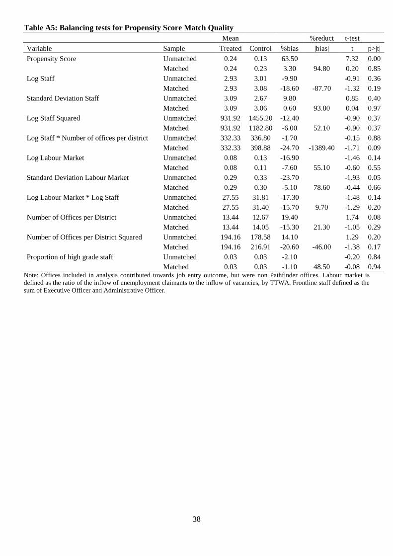
38

Table A5: Balancing tests for Propensity Score Match Quality Mean %reduct t-test Variable Sample Treated Control %bias |bias| t p>|t| Propensity Score Unmatched 0.24 0.13 63.50 7.32 0.00 Matched 0.24 0.23 3.30 94.80 0.20 0.85 Log Staff Unmatched 2.93 3.01 -9.90 -0.91 0.36 Matched 2.93 3.08 -18.60 -87.70 -1.32 0.19 Standard Deviation Staff Unmatched 3.09 2.67 9.80 0.85 0.40 Matched 3.09 3.06 0.60 93.80 0.04 0.97 Log Staff Squared Unmatched 931.92 1455.20 -12.40 -0.90 0.37 Matched 931.92 1182.80 -6.00 52.10 -0.90 0.37 Log Staff * Number of offices per district Unmatched 332.33 336.80 -1.70 -0.15 0.88 Matched 332.33 398.88 -24.70 -1389.40 -1.71 0.09 Log Labour Market Unmatched 0.08 0.13 -16.90 -1.46 0.14 Matched 0.08 0.11 -7.60 55.10 -0.60 0.55 Standard Deviation Labour Market Unmatched 0.29 0.33 -23.70 -1.93 0.05 Matched 0.29 0.30 -5.10 78.60 -0.44 0.66 Log Labour Market * Log Staff Unmatched 27.55 31.81 -17.30 -1.48 0.14 Matched 27.55 31.40 -15.70 9.70 -1.29 0.20 Number of Offices per District Unmatched 13.44 12.67 19.40 1.74 0.08 Matched 13.44 14.05 -15.30 21.30 -1.05 0.29 Number of Offices per District Squared Unmatched 194.16 178.58 14.10 1.29 0.20 Matched 194.16 216.91 -20.60 -46.00 -1.38 0.17 Proportion of high grade staff Unmatched 0.03 0.03 -2.10 -0.20 0.84 Matched 0.03 0.03 -1.10 48.50 -0.08 0.94

Note: Offices included in analysis contributed towards job entry outcome, but were non Pathfinder offices. Labour market is defined as the ratio of the inflow of unemployment claimants to the inflow of vacancies, by TTWA. Frontline staff defined as the sum of Executive Officer and Administrative Officer.