
SimCCSK: Simulation of the Reversible Process … · SimCCSK: Simulation of the Reversible Process...
108
SimCCSK: Simulation of the Reversible Process Calculi CCSK by Gavin Cox Submitted for the degree of Master of Philosophy at the University of Leicester 2008
Transcript of SimCCSK: Simulation of the Reversible Process … · SimCCSK: Simulation of the Reversible Process...
SimCCSK: Simulation of the
Reversible Process Calculi CCSK
by
Gavin Cox
Submitted for the degree of
Master of Philosophy
at the University of Leicester
2008

ii
Abstract
Reversibility is becoming a more common trend in computer science research. This
research ranges from programming languages through to process calculi. It is process
calculi that we are interested in here. Reversibility of Milner’s CCS has been studied by
both Danos and Krivine with their process calculus RCCS as well as by Phillips and
Ulidowski with theirs called CCSK.
We describe research in the simulation of Phillips and Ulidowski’s CCSK. We primarily
look at this from the standpoint of creating a tool for use within the academic sector,
specifically the aiding of undergraduate students trying to learn process calculi. We
will look into how we can represent the data associated with agents within the context
of a computer simulator. We also look at how we can implement the operational
semantics giving us the transitions between states within this system. Also we shall
see how a Graphical User Interface that contains the relevant information in a clear
and concise manner is an important part of making the tool more accessible to
undergraduate students.
We will present both SimCCSK and WinSimCCS. SimCCSK is a prototype command line
driven simulator for CCSK which includes the key operations and features of CCSK and
allows for the user driven simulation of CCSK agents. WinSimCCSK is a graphical
prototype version built on the same core engine from SimCCSK and contains all of the
same features. WinSimCCSK also includes some additional features such as a built-in
“Agent Editor” allowing easier creation and editing of agents and a dynamically
generated graph based visualisation of the agent’s transitions. It also includes an
“Automatic Simulation” feature for the automatic generation of the visualisation for
teaching examples. Finally, we will look at how this information can be presented and
interacted with in order to make the whole system clear to students helping them
reinforce the traditional learning process and present a few examples illustrating its
action.

iii
Acknowledgements
I would like to acknowledge the staff and students of the Department of Computer
Science at the University of Leicester for all the encouragement and advice. My thanks
go to my family for their support during my work on this, in particular my parents
Janice and Peter. Finally, I would like to thank Sarah, Andy and Martin for their
support during this.

iv
Contents
Contents ............................................................................................................. iv
List of Figures .................................................................................................... vii
1. Introduction ........................................................................................................ 1
1.1 Context of Thesis ............................................................................................ 1
1.2 Challenges ...................................................................................................... 2
1.3 Outline of Solution ......................................................................................... 4
1.4 Structure of Thesis ......................................................................................... 5
2. Background ......................................................................................................... 6
2.1 Basics of CCS ................................................................................................... 6
2.1.1 SOS Rules of CCS ................................................................................... 10
2.1.2 Examples ............................................................................................... 11
2.2 Basics of RCCS ............................................................................................... 12
2.3 Basics of CCSK ............................................................................................... 15
2.3.1 SOS Rules of CCSK ................................................................................. 19
2.4 CCSK vs. RCCS: A Comparison...................................................................... 21
2.5 Conclusions .................................................................................................. 24
3. Design ............................................................................................................... 25
3.1 Requirements ............................................................................................... 25
3.1.1 Quality Requirement Details................................................................. 26
3.2 Concept ........................................................................................................ 27
3.3 Internal Data Structures ............................................................................... 31
3.4 Implementation Language ........................................................................... 33
3.5 Related Work ................................................................................................ 36

v
3.5.1 CWB-NC ................................................................................................. 36
3.5.2 FDR2 ...................................................................................................... 37
3.5.3 Comparison with SimCCSK .................................................................... 38
3.6 Graphical User Interface Concept ................................................................ 40
3.7 Conclusions .................................................................................................. 42
4. Implementation ................................................................................................. 43
4.1 Laying the Ground Work .............................................................................. 43
4.2 Construction of the Internal Data Structure ................................................ 45
4.3 Putting it Together ....................................................................................... 50
4.4 Conclusions .................................................................................................. 52
5. WinSimCCSK ...................................................................................................... 53
5.1 SimCCSK for a More Colourful World .......................................................... 53
5.2 Examples ...................................................................................................... 59
5.2.1 The DNA System ................................................................................... 59
5.2.2 The Jobshop .......................................................................................... 67
5.2.3 The Dining Philosophers ....................................................................... 73
5.3 Conclusions .................................................................................................. 78
6. User Guide ......................................................................................................... 79
6.1 Requirements ............................................................................................... 79
6.2 Setting up WinSimCCSK ................................................................................ 79
6.2.1 WinSimCCSK Main Screen ..................................................................... 80
6.2.2 Agent Editor .......................................................................................... 81
6.2.3 Making a Move ..................................................................................... 83
6.3 Automatic Simulation ................................................................................... 84
6.4 Tutorial Example – a.b.0 ............................................................................... 85

vi
7. Critical Appraisal................................................................................................ 89
7.1 SimCCSK – A Simulator for CCSK? ................................................................ 89
7.2 WinSimCCSK – SimCCSK for All? ................................................................... 91
7.3 Possible Extensions to the Project ............................................................... 93
8. Conclusions ....................................................................................................... 95
8.1 SimCCSK as a Simulator for CCSK ................................................................. 95
8.2 WinSimCCSK as a Tool for Teaching ............................................................. 96
8.3 Final Thoughts .............................................................................................. 97
Bibliography ...................................................................................................... 98

vii
List of Figures
Figure 2.1-1: SOS Rules for CCS ...................................................................................... 10
Figure 2.3-1: SOS Rules for the std(X) Relation .............................................................. 19
Figure 2.3-2: Forward SOS Rules for CCSK ...................................................................... 20
Figure 2.3-3: Reverse SOS Rules for CCSK ....................................................................... 21
Figure 3.2-1: Concept of Action and Agent .................................................................... 28
Figure 3.2-2: Concept of Action, Agent and Simulator ................................................... 28
Figure 3.2-3: Concept of Agent Hierarchy ...................................................................... 28
Figure 3.2-4: Inheritance Concept Class Diagram ........................................................... 29
Figure 3.2-5: Inheritance Concept Class Diagram (Part 2) .............................................. 30
Figure 3.2-6: Inheritance Concept Class Diagram (Part 3) .............................................. 31
Figure 3.3-1: Constructing a.b.0 using a simple approach ............................................. 31
Figure 3.3-2: Constructing a.b.0 + c.d.0 using a simple approach .................................. 32
Figure 3.5-1: Comparison of SimCCSK, CWB-NC and FDR2 ............................................ 38
Figure 3.6-1: Mock up of WinSimCCSK Main Form ........................................................ 41
Figure 3.6-2: GUI State Diagram ..................................................................................... 42
Figure 4.1-1: Class Structure of SimCCSK Core (part 1) .................................................. 44
Figure 4.1-2: Class Structure of SimCCSK Core ............................................................... 44
Figure 4.2-1: AST Implementation Example Class Diagram ............................................ 45
Figure 4.2-2: Code for ChoiceAgent.MakeMove() .......................................................... 46
Figure 4.2-3: Pseudo code for Prefix.MakeMove() ......................................................... 47
Figure 4.2-4: Calling MakeMove() and Updating "current" Agent ................................. 48
Figure 4.2-5: State Diagram for MakeMove() ................................................................. 48
Figure 4.3-1: Example of SimCCSK interface (a.b.0 + c.d.0)............................................ 51
Figure 4.3-2: Example of SimCCSK interface (a.b.0 + ‘a.c.0) ........................................... 52
Figure 5.1-1: WinSimCCSK Main Form ............................................................................ 55
Figure 5.1-2: Pseudo code for "absolute" Agent Generation ......................................... 58
Figure 5.2-1: Illustration of Gene Expression ................................................................. 60
Figure 5.2-2: Complete DNA Graph ................................................................................ 63
Figure 5.2-3: DNA Graph at depth of 2 ........................................................................... 63

viii
Figure 5.2-4: Trace of A and I1 binding on DNA ............................................................. 65
Figure 5.2-5: Trace back tracking binding of I1 to allow expression of gene ................. 67
Figure 5.2-6: Jobshop graph at depth 1 .......................................................................... 68
Figure 5.2-7: Jobshop graph at depth 2 .......................................................................... 69
Figure 5.2-8: Jobshop Graph at depth 3 ......................................................................... 70
Figure 5.2-9: Data Collected from Jobshop .................................................................... 72
Figure 5.2-10: Dining Philosophers Deadlock Resolve graph ......................................... 76
Figure 5.2-11: Dining Philosophers Deadlock Resolve graph with additional route ...... 77

1
Chapter 1
Introduction
1.1 Context of Thesis
Process calculi have long been used as a method of modelling concurrent systems. In
the 1970s Milner created the Calculus of Communicating Systems (CCS) (1). There is a
long running trend to investigate the use of reversibility (2) (3). Process calculi are no
exception. The reasoning is due to the wide number of possible uses for reversibility
in computing. There are many well known examples, including biological system
modelling and transactions in service oriented computing through to reversible
debugging. Biological system modelling involves reversibility as biological systems by
their very nature are reversible and so, therefore, the model should be able to cope
with this natural reversibility. In the case of transactions in service oriented
computing, reversibility comes into play when a series of events or transactions fail to
complete midway through the process and therefore need to reverse back to a point
where another sequence can be executed Alternative approaches to this transaction
failure include compensation. Compensation is where instead of reversing back to a
point, a sequence of events are triggered to reset the specific events or transactions
which had been executed previously. Another example is reversible debugging, since
the current issues with debugging revolve around a computer’s inability to recover
from an application crash. Reversibility would allow the debugger to reverse the steps
leading up to the crash allowing for the creation of a more informative state of the
2
system leading up to the crash. Even more intriguing is something Landauer wrote
back in 1961 on reversibility, in a paper he noted that it is not the computation but the
deletion of information that generates an increase in entropy and thus dissipates heat
(4), what this would mean is that if every action a computer made was reversible we
would never need to erase it and therefore the heat generated would be far lower.
This could then lead to higher clock speeds due to the increased space in temperature.
In the case of CCS we can now see two extensions to CCS that add reversibility, one by
Danos and Krivine called Reversible CCS (RCCS) and another by Phillips and Ulidowski,
CCS with Keys (CCSK). We are going to look into a sub-area to this, related to the
computer simulation of process calculi; specifically the objective is to develop a
simulator for CCSK to be possibly used in the reinforcement of learning by students
studying about process calculi.
1.2 Challenges
Currently there is very little work concerning the design and construction of a
simulator for reversible process calculi and particularly in the case of CCSK. Existing
process calculi simulators deal only in non-reversible calculi. Two examples of these
are Concurrency Workbench of New Century (CWB-NC), which is primarily CCS-based
and FDR2 for CSP. Both tools have features that are useful, however, are not really
suited to aiding student experimentation and learning. Whilst CWB-NC does have a
graphical representation of a system, it is only trace based which means only the route
taken is shown. Also due to it using CCS it has no real reversibility and, therefore, lacks
the ability to show students how alternative choices alter the behaviour of a system.
FDR2 on the other hand has no graphical representation, again has no real
reversibility, and is therefore lacking the features required for students. What both
tools have in common and really shows the main objective of these applications, is
model checking. They are inherently designed to check systems as opposed to be
interactive simulators; the interactive simulation is more of an add-on as opposed to
the primary function.

3
So the challenges of this project are based around the creation of an interactive
simulator that could be used in the teaching of students, allowing them to explore and
interact with a system to gain a deeper understanding of process calculi. We feel that
this gives us two key challenges:
• Implementation of the Operational Semantics
• Graphical User Interface Design
Of course being inherently a software oriented project, a key challenge is how we can
represent and interact with agents (being a key construct in CCSK) within the realm of
software. It has to be both well designed so that it is clear to the software what the
agent is, as well as being flexible enough to cope with the variants of agents within
CCSK. Once we have an internal representation, we need to be able to interact with it
and make various transitions between the states of the agent. These transitions are
defined by the operational semantics, it is a key challenge to design and implement
these so that they operate in a consistent and intended way. As previously mentioned,
our aim is that this simulator is accessible to students learning process calculi. This
leads us to our second key challenge, the graphical user interface (GUI) design. We
feel that for students learning process calculi, the simulator should help them with just
that. We feel that it should not be a requirement to understand an intricate and
overly complicated system to learn and experiment with process calculi. To this end,
we feel that the GUI should present all of the relevant information in an easy to
understand way, whilst maintain a simple to pick up and use piece of software.

4
1.3 Outline of Solution
In this thesis we will present our solution to the above challenges, culminating in a
working prototype of a CCSK simulator called WinSimCCSK. We will also show a few
examples with this tool highlighting its functionality; these examples include the classic
CCS Jobshop, a biological system and the classic Dining Philosophers.
We will show how we internally represent agents (collectively known as a system).
This is achieved using an almost static tree like structure, which we combine with keys
and pointers to provide the current state of the system. The idea behind this
approach to the solution is due to the almost static nature of the internal structure,
that all previous states can be captured with this single structure. This also gives the
added benefit that the amount of memory used for storage of the state of the system
is restricted due to its limited size which is based on the size of the agent not on the
transitions between them.
For the operational semantics, we show how through the uses of inheritance and
polymorphism we can create a simple yet dynamic framework as a base for the
operational semantics. This allows the various rules to be defined separately and yet
be called dynamically at runtime from an agent. The agent does not need to know
which rule to call, as this is all resolved dynamically through polymorphism aided by
common data defined with the aid of inheritance.
The GUI is designed to be intuitive and easy to read. To this end we have created a
GUI which not only contains the current state of the system, but also lists the possible
forward and reverse moves in a clear and concise fashion. In order to aid student
learning we felt a graphical representation was important, so we include a graph
which is dynamically created as the user makes various moves showing the transitions
between the various states of the system. In order to make the systems easy to pick
up and use, we also include a simple “Agent Editor” which allows CCSK agents to be
defined for use within the simulator and can be saved for future reuse, as well as an
“Automatic Simulation” function which automatically generates the transition graph of
the system up to a user specified depth.

5
1.4 Structure of Thesis
This thesis is organised as follows. In chapter 2 we shall look at the background of the
project, specifically looking as CCS, RCCS and CCSK with a small comparison between
RCCS and CCSK. Chapter 3 will look that the designs of the software, including the
requirements, concept and how the data can be represented, as well as a brief look at
related work. Chapter 4 will look at the implementation details of SimCCSK including
the internal data structure and console based interface. Chapter 5 goes on to outline
WinSimCCSK, the graphical version, looking at its extended features and user
interface. We then go on to look at a few examples with the help of WinSimCCSK.
Chapter 6 provides a concise user guide to WinSimCCSK, outlining how one can use
the prototype. Chapter 7 looks what the project has achieved against its original aims.
Finally, in Chapter 8 there is a review of the thesis with conclusions.
6
Chapter 2
Background
Over the course of this chapter we shall look at some of the background to the project
including a brief look at CCS, RCCS and CCSK. Finally we shall end the chapter with a
concise comparison between RCCS and CCSK, looking at our reasoning behind basing
this project on CCSK.
2.1 Basics of CCS
Calculus of Communicating Systems (CCS) was created by Milner in the early 70’s for
modelling concurrent systems. In this section we will identify some of the ideas,
concepts and constructs of CCS.
CCS is specified by the following BNF grammar:
� ∶∶= 0 | �. � | � + �� | �|�� | �[ /�] | �\� | �
where
0 is the zero agent
�. � is the action � followed by the agent �
� + �� is the choice of � or ��
�|�� is parallel composition and means both � and �� can be used
�[ /�] is relabeling and means all actions � in � are renamed to
�\� is restriction of the action � in �
� is an agent identifier. � = � means � refers to the agent �
7
The simplest construct in CCS is that of the Zero agent (written simply as ‘0’). The Zero
agent is simply a terminated agent. It can do nothing and it is often the terminating
point in more complex CCS agents.
The second operator is the Prefix (denoted by a ‘.’). The Prefix operator specifies the
transition between an agent �. � and � by the execution of the action �. A simple
example of this is if we take the action � and the Zero agent, the resulting Prefix agent
would be �. 0 which would specify the transition to 0 by the execution of action �.
Equally, prefixing the action to the resulting agent would result in . �. 0. This now
gives us a route to 0 by the execution of , resulting in the transition to �. 0 and then �
to 0.
The Choice operator (denoted by a ‘+’) allows for two (or more) agents to be
combined together to form a choice between them. A simple example of this is if we
take the agents �. 0 and . 0 and combine via the Choice resulting in the agent
is �. 0 + . 0. The Choice is destructive in the sense that once a path is chosen the
other is no longer available. An example of this is if we take the agent �. . 0 + �. �. 0.
If we perform the action �, giving us the transition to . 0, we would have lost access
to the agent �. �. 0. The Choice agent is usually seen as a binary construct. However
this is usually for the sake of convenience and is referred to as "Finite Summation" (1).
It is formally defined in (1) as ∑ ���∈� , basically this states that for a set of indices � we
can sum together the collection of agents ��. Choice is also both commutative and
associative, i.e. � + � = � + � (commutative) and � + �� + �� = �� + �� + �
(associative).
In order to facilitate concurrency, CCS uses the Parallel operator (denoted by a ‘|’).
The Parallel operator allows two (or more) agents to combine in a parallel and
concurrent fashion. A simple example of this is if we take the agents �. 0 and . 0 and
combine via the Parallel, resulting in the agent is �. 0 | . 0. Unlike Choice, Parallel is
non-destructive in the sense that if we follow one path, the other is still open to us.
An example of this is if we take the agent �. . 0 | �. �. 0 and perform action �, we get
a transition to . 0 | �. �. 0, so we would still have access to the agent �. �. 0. More
often than not we will want to combine more than two agents in Parallel, this can be
8
done e.g. �. 0 | . 0 | �. 0. However like Choice, the Parallel agent is usually seen as a
binary construct. Again this is more out of convenience as we can combine two
together and then keep putting the resulting agent in parallel with another (E::= E|E).
Parallel is also both commutative and associative, i.e. � | � = � | � (commutative)
and � | �� | �� = �� | �� | � (associative).
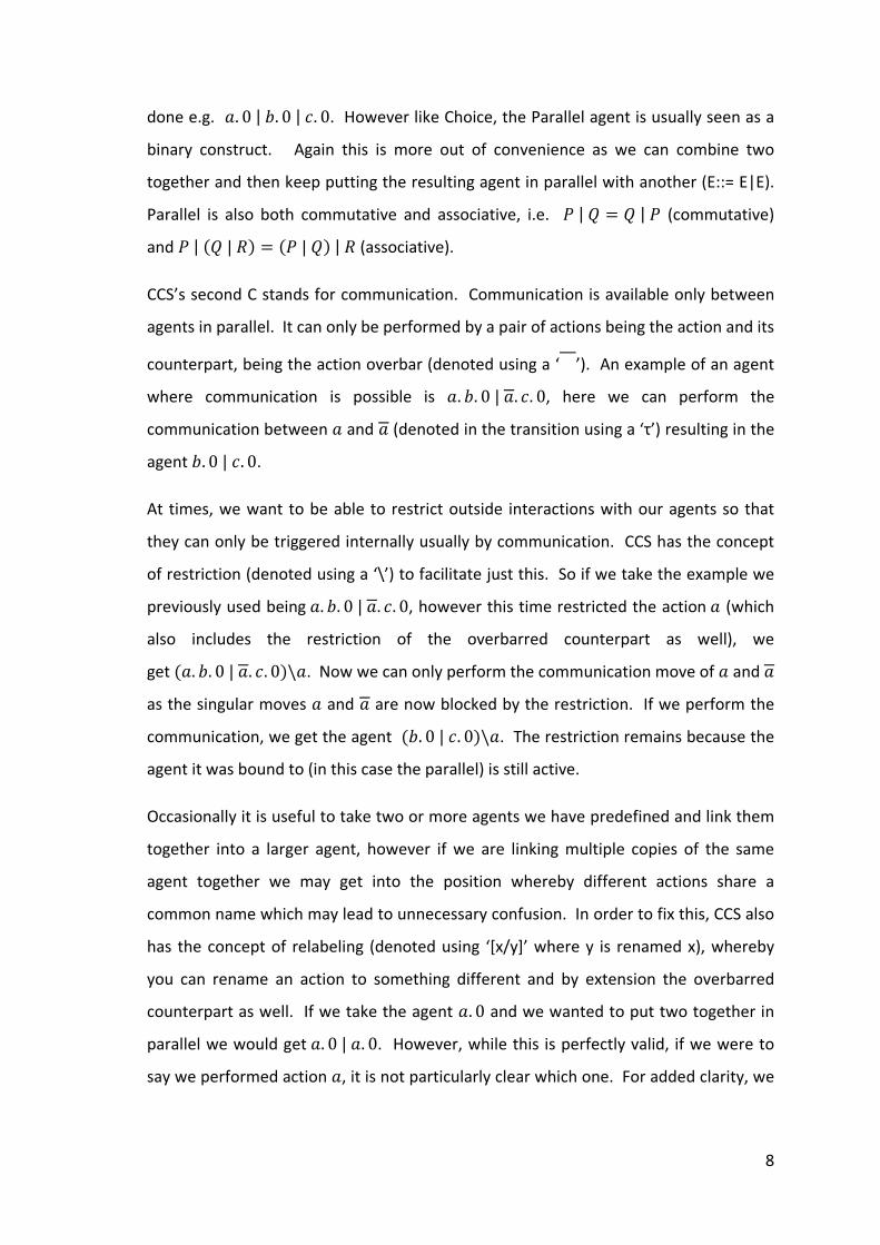
CCS’s second C stands for communication. Communication is available only between
agents in parallel. It can only be performed by a pair of actions being the action and its
counterpart, being the action overbar (denoted using a ‘ ’). An example of an agent
where communication is possible is �. . 0 | �. �. 0, here we can perform the
communication between � and � (denoted in the transition using a ‘τ’) resulting in the
agent . 0 | �. 0.
At times, we want to be able to restrict outside interactions with our agents so that
they can only be triggered internally usually by communication. CCS has the concept
of restriction (denoted using a ‘\’) to facilitate just this. So if we take the example we
previously used being �. . 0 | �. �. 0, however this time restricted the action � (which
also includes the restriction of the overbarred counterpart as well), we
get ��. . 0 | �. �. 0�\�. Now we can only perform the communication move of � and �
as the singular moves � and � are now blocked by the restriction. If we perform the
communication, we get the agent � . 0 | �. 0�\�. The restriction remains because the
agent it was bound to (in this case the parallel) is still active.
Occasionally it is useful to take two or more agents we have predefined and link them
together into a larger agent, however if we are linking multiple copies of the same
agent together we may get into the position whereby different actions share a
common name which may lead to unnecessary confusion. In order to fix this, CCS also
has the concept of relabeling (denoted using ‘[x/y]’ where y is renamed x), whereby
you can rename an action to something different and by extension the overbarred
counterpart as well. If we take the agent �. 0 and we wanted to put two together in
parallel we would get �. 0 | �. 0. However, while this is perfectly valid, if we were to
say we performed action �, it is not particularly clear which one. For added clarity, we

9
can change the second one from an � to a thereby easily distinguishing between the
two choices. This would give us a new agent �. 0 | � . 0�[ /�].
A more concrete example of this would be if we had a �� !" agent defined as
#$%&&. �� !". Now we can put two buttons together, for example (in an example
inspired by (1)) in a vending machine for chocolate (which can dispense a standard and
large bars) with a button for each size. However currently we would have
#$%&&. �� !" | #$%&&. �� !" which makes it unclear which button relates to which
size. Using renaming we can make this clearer by altering the names of the buttons,
for example:
#$%&&' �. �� !" [#$%&&' � / #$%&&] | #$%&&($). �� !" [#$%&&($) / #$%&&]
An alternative example is one where communication is possible. Taking our previous
example, we want the button to trigger the dispensing of the chocolate. This time
however we shall simplify the example by only having one type of chocolate bar. We
will also update the �� !" agent to include a !� signal (showing the button has
been pressed), which we shall define as #$%&&. !� . �� !". We will also include
*+&#%"&% agent defined as �+&#%"&%. �$!#�ℎ!�. *+&#%"&%. We want the two to
communicate, so that when the button is pressed we trigger the dispense mechanism
and the chocolate is dropped (as signified by the �$!#�ℎ!� action). To do this we put
them together in parallel, resulting
in #$%&&. !� . �� !" | �+&#%"&%. �$!#�ℎ!�. *+&#%"&%. The issue with this is that
they cannot communicate because !� and �+&#%"&% are not a matching pair. We
solve this by renaming one of the actions to match the other, so if we rename the !�
to �+&#%"&% we would get
�#$%&&. !� . �� !"�[�+&#%"&%/!� ] | �+&#%"&%. �$!#�ℎ!�. *+&#%"&% which would
now allow communication as we now have a matching pair, being �+&#%"&% and !�
which has been renamed �+&#%"&%.

10
2.1.1 SOS Rules of CCS
CCS’s transitional rules can be expressed using Plotkin’s Structural Operational
Semantics (SOS) (5) (6). So for reference the SOS rules are included below.
�$%-+. �. / 0→ /
2ℎ!+�% / 0→ /3
/ + 4 0→ /3 4 0→ 43
/ + 4 0→ 4′
��$�66%6 / 0→ /3
/ | 4 0→ /3 | 4 4 0→ 43
/ | 4 0→ / | 4′
2!77�"+�� +!" / 0→ /3 4 0→ 43 / | 4 8→ /3 | 4′
�� ≠ :�
�%& $+� +!" / 0→ /3
/ \ � 0→ /3 \ � � ∉ � ∪ �
�%6� %66+") / 0→ /3
/[-] =�0�>?@ /3[-]
Aℎ%$% /[-] = / $%"�7%� B -�"� +!" -
�%��$&+!" / ≡ 4 4 0→ 43 4′ ≡ /′/ 0→ /′
Figure 2.1-1: SOS Rules for CCS

11
2.1.2 Examples
We will now show a few simple examples illustrating CCS with the aid of the SOS rules.
Our first example is of prefix, taking �. . 0. From start to finish this agent has two
transitions shown below.
�. . 0 0→ . 0 and . 0 D→ 0
This example uses a single SOS rule (being prefix). The rule simply states that an agent
with a prefixed action can make the transition to the agent by performing the action.
So here �. . 0 is � prefixed on to . 0 can make the transition by performing the
�. . 0 works similarly.
Our second example is one involving parallel, �. . 0 | �. �. 0. From this state we have
two transitions:
�. . 0 E �. �. 0 0→ . 0 E �. �. 0 and �. . 0 E �. �. 0 F→ �. . 0 E �. 0
This time round in the first instance we look at the parallel rules. The rules state that
we can make the transition if either side of the parallel can make a transition, so in our
case �. . 0 or �. �. 0 can make a transition. Clearly these can apply the prefix rule we
saw earlier. The parallel also states the result of the transition is the result of the
agent that made the transition in parallel with the unaltered other agent. In our
example this gave us . 0 | �. �. 0 if we performed the � (of �. . 0) and �. . 0 | �. 0 if
we performed the � (of �. �. 0).
Our final example is a simple recursive one, being � with � = �. �. Here we have a
single transition:
� 0→ �
This transition does look a little odd at first sight, the reason for this is that both sides
of the transition are the same. This however does make a lot of sense in reality. If we

12
look at what is happening, we can see that the � is defined as �. � so we really have
the following transition:
�. � 0→ �
This transition is of course a simple prefix and shows that � does in fact have a
transition to � with the action �. Of course what has really happened is that we have
replaced the � agent with an actual instance of �. �. As such subsequent transitions
would be different �'s as opposed to repeatedly performing the same one.
2.2 Basics of RCCS
Danos and Krivine have created a way of adding reversibility to CCS (7) (8) (9), by
utilising the concept of a memory stack using the notion of pushing previous data onto
the stack so that it can be popped off in the event of a roll back. We shall now look at
the ideas and constructs of RCCS.
Let us look at the Prefix agent in RCCS. Here we will use an example �. . 0 to help
visualise and explain the process.
[�. . 0],H,0>?@< $, �, 0 >. [ . 0]
This one transition makes the forward move of �. As we can see this is slightly more
complex than the CCS version due to the added information required in order to
facilitate the reverse move. The label of the transition (being 1, $, �) is made up of
three parts, the first being the 1; this is the process label which identifies which
process the transition is being actioned on. In this example with only one process it is
of little relevance, however, with two or more processes it gains usefulness. Second is
the $, which is just a label for ease of reference. Finally the �, which is the action
performed.
The resulting agent is both the CCS equivalent (in this case . 0) and the created stack
(notated using < >). In the stack there are three parts; the label ($), the action

13
performed (�) and any ‘lost’ agents. In our case because it is a simple Prefix agent and
therefore with no other agents to lose, we use the Zero agent (0).
Now let us look at the reverse move, using the same example.
< $, �, 0 >. [ . 0].H.0L?M [�. . 0]
Here we see that the label and action are both in the stack and the transition
effectively links the two. The process label again matches the transition to a process.
It is worth noting that the transition does in fact go from left to right; the transition
arrow (going from right to left) just signifies that we are performing a reverse move.
The resulting agent is constructed by adding the action to the front of the process and
by then adding any lost agents. However in our case due to there being no lost agents
(signified by the Zero agent), none are added.
Choice is also in RCCS, again we will use an example this being �. . 0 + �. �. 0 to help
visualise and explain the process.
[�. . 0 + �. �. 0],H,0>?@< $, �, �. �. 0 >. [ . 0]
This single transition shows the execution of the forward action �. As in the previous
example we still have the transition label (being 1, $, �) which has the same meaning.
The key difference here is that in our resulting agent we now have a ‘lost’ agent (being
�. �. 0) so whereas in our previous example the third part of the stack was set to be
empty (notated by the Zero agent), there is now something on it, this being the lost
agent.
Look at how this affects the reverse move.
< $, �, �. �. 0 >. [ . 0],H,0L?M [�. . 0 + �. �. 0]
Once again the transition label is the same as our previous example (as we are still
performing action �); the key difference here is clearly the stack and more specifically
the third part of it. This time around we have a ‘lost’ agent to re-attach to the
resulting agent. This is created by adding the previous action to the front of the agent.
14
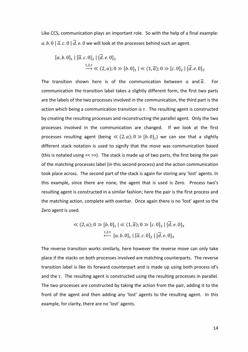
Like CCS, communication plays an important role. So with the help of a final example:
�. . 0 | �. �. 0 | �. %. 0 we will look at the processes behind such an agent.
[�. . 0] | [�. �. 0]� | [�. %. 0]N,�,8>?@ ≪ �2, ��; 0 ≫ [ . 0] | ≪ �1, ��; 0 ≫ [�. 0]� | [�. %. 0]N
The transition shown here is of the communication between � and �. For
communication the transition label takes a slightly different form, the first two parts
are the labels of the two processes involved in the communication, the third part is the
action which being a communication transition is :. The resulting agent is constructed
by creating the resulting processes and reconstructing the parallel agent. Only the two
processes involved in the communication are changed. If we look at the first
processes resulting agent (being ≪ �2, ��; 0 ≫ [ . 0]) we can see that a slightly
different stack notation is used to signify that the move was communication based
(this is notated using << >>). The stack is made up of two parts, the first being the pair
of the matching processes label (in this second process) and the action communication
took place across. The second part of the stack is again for storing any ‘lost’ agents. In
this example, since there are none, the agent that is used is Zero. Process two’s
resulting agent is constructed in a similar fashion; here the pair is the first process and
the matching action, complete with overbar. Once again there is no ‘lost’ agent so the
Zero agent is used.
≪ �2, ��; 0 ≫ [ . 0] | ≪ �1, ��; 0 ≫ [�. 0]� | [�. %. 0]N ,�,8L?M [�. . 0] | [�. �. 0]� | [�. %. 0]N
The reverse transition works similarly, here however the reverse move can only take
place if the stacks on both processes involved are matching counterparts. The reverse
transition label is like its forward counterpart and is made up using both process id’s
and the :. The resulting agent is constructed using the resulting processes in parallel.
The two processes are constructed by taking the action from the pair, adding it to the
front of the agent and then adding any ‘lost’ agents to the resulting agent. In this
example, for clarity, there are no ‘lost’ agents.

15
2.3 Basics of CCSK
CCSK is another approach to adding reversibility to Milner’s CCS, introduced by Phillips
and Ulidowski (10) (11) (12) (13) and is based on the use of keys to both signify past
actions and to lock communicating actions together. In this section we will look at the
ideas and constructs of CCSK.
CCSK is specified by the following BNF grammar:
� ∶∶= 0 | �. � | �[S]. �| � + �� | �|�� | �[ /�] | �\� | �
where
0 is the zero agent
�. � is the action � followed by the agent �
�[S]. � is the past action � with key S followed by the agent �
� + �� is the choice of � or ��
�|�� is parallel composition and means both � and �� can be used
�[ /�] is relabeling and means all actions � in � are renamed to
�\� is restriction of the action � in �
� is an agent identifier. � = � means � refers to the agent �
The Prefix agent in CCSK is very similar to its CCS counterpart. The key difference
between the two is the introduction of a key which is used to signify past actions and,
as described later, also binds two agents together in communication. In order to help
illustrate the CCSK approach to Prefix we shall look at the simple example of �. . 0.
�. . 0 0[T]>?@ �[S]. . 0
The transition is labelled by the action and the key (in the example S is a unique key)
being assigned to that action (denoted in [ ]). The result is the previous agent with the
new key now associated to the action that has just been performed. This move can
only be made however if the rest of the result, the part following the action performed
(in this example . 0) is a 'standard' CCS agent, i.e. it does not contain any keys.

16
The reversed counterpart is similar.
�[S]. . 0 ⇝0[T]�. . 0
Here we see the transition is labelled again with the action and the key, however to
signify the reverse nature of the move a squiggled arrow ⇝ is used. The resulting
agent is the agent with the key removed from the action performed.
Like CCS and RCCS, CCSK also has the notion of choice; in fact like most of CCSK it is
very similar to its CCS counterpart. An example of this is �. . 0 + �. �. 0.
�. . 0 + �. �. 0 0[T]>?@ �[S]. . 0 + �. �. 0
The transition is again labelled with the action and a key. The resulting agent is the
key added to the performed action. The other part of the choice is left infix, however
the choice rule states that the other part of the choice is a ‘standard’ CCS agent (i.e. it
contains no past actions). It would be impossible to perform an action from the other
side i.e. �. �. 0 as this would now be locked as �[S]. . 0 is not a ‘standard’ CCS agent
as it uses a key.
In reverse Choice works similarly; using the example above we get.
�[S]. . 0 + �. �. 0 ⇝0[T] �. . 0 + �. �. 0
The transition is once again labelled with the action and the key. The resulting agent is
simply generated by removing the key from the action that has just been performed.
Again like its forward counterpart the rule for reverse choice again requires that the
other part of the choice is a ‘standard’ CCS agent. In practice you should not really be
in the position where both parts of the choice are non-standard, i.e. contain keys. If
this was the case this would mean you had violated the forward transition rule, as
somehow you would have actioned both sides of the choice (meaning you had
effectively treated them as agents in parallel).
17
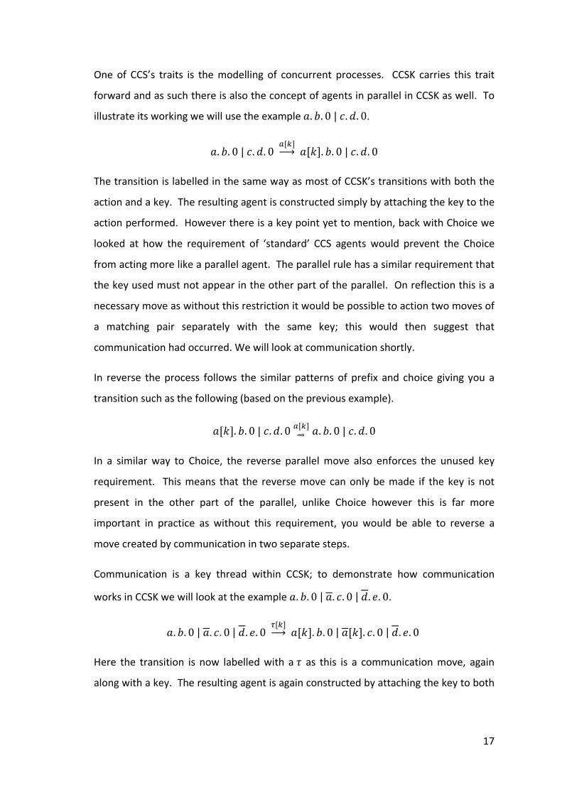
One of CCS’s traits is the modelling of concurrent processes. CCSK carries this trait
forward and as such there is also the concept of agents in parallel in CCSK as well. To
illustrate its working we will use the example �. . 0 | �. �. 0.
�. . 0 | �. �. 0 0[T]>?@ �[S]. . 0 | �. �. 0
The transition is labelled in the same way as most of CCSK’s transitions with both the
action and a key. The resulting agent is constructed simply by attaching the key to the
action performed. However there is a key point yet to mention, back with Choice we
looked at how the requirement of ‘standard’ CCS agents would prevent the Choice
from acting more like a parallel agent. The parallel rule has a similar requirement that
the key used must not appear in the other part of the parallel. On reflection this is a
necessary move as without this restriction it would be possible to action two moves of
a matching pair separately with the same key; this would then suggest that
communication had occurred. We will look at communication shortly.
In reverse the process follows the similar patterns of prefix and choice giving you a
transition such as the following (based on the previous example).
�[S]. . 0 | �. �. 0 ⇝0[T] �. . 0 | �. �. 0
In a similar way to Choice, the reverse parallel move also enforces the unused key
requirement. This means that the reverse move can only be made if the key is not
present in the other part of the parallel, unlike Choice however this is far more
important in practice as without this requirement, you would be able to reverse a
move created by communication in two separate steps.
Communication is a key thread within CCSK; to demonstrate how communication
works in CCSK we will look at the example �. . 0 | �. �. 0 | �. %. 0.
�. . 0 | �. �. 0 | �. %. 0 8[T]>?@ �[S]. . 0 | �[S]. �. 0 | �. %. 0
Here the transition is now labelled with a : as this is a communication move, again
along with a key. The resulting agent is again constructed by attaching the key to both

18
of the matching pair of actions (i.e. action and action overbar, with action overbar
being the same as in CCS) performed thus locking the two agents and actions together.
The reverse equivalent looks like this.
�[S]. . 0 | �[S]. �. 0 | �. %. 0 ⇝8[T] �. . 0 | �. �. 0 | �. %. 0
Again the transition is labelled with a : along with a key. The resulting agent is
constructed by removing the keys from both actions of the matching pair which make
up the communication move. The important point here is that the key must be
identical on both parts of the matching pair of actions.
Finally like CCS, CCSK also has the notions of restriction and relabeling and they
operate in the same way as CCS for the forward moves. For the reverse moves they
operate in exactly the same way as one would expect, however like the rest of CCSK
reverse moves, the ‘reverse’ transitions for both relabeling and restriction are notated
using the squiggled arrow ⇝.
19
2.3.1 SOS Rules of CCSK
Like CCS, CCSK’s transition rules can also be expressed using Plotkin’s Structural
Operational Semantics. So for reference and possible comparison we shall include the
SOS rules below.
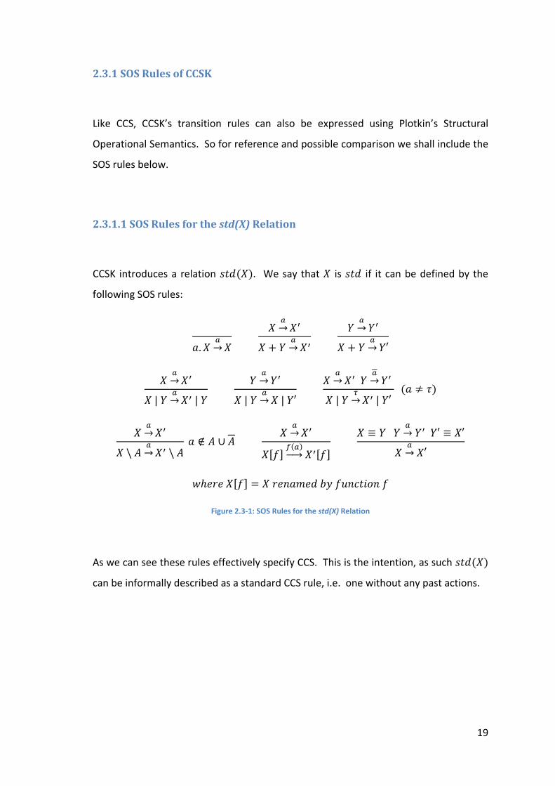
2.3.1.1 SOS Rules for the std(X) Relation
CCSK introduces a relation & ��/�. We say that / is & � if it can be defined by the
following SOS rules:
�. / 0→ / / 0→ /3
/ + 4 0→ /3 4 0→ 43
/ + 4 0→ 4′
/ 0→ /3
/ | 4 0→ /3 | 4 4 0→ 43
/ | 4 0→ / | 4′ /
0→ /3 4 0→ 43 / | 4 8→ /3 | 4′
�� ≠ :�
/ 0→ /3
/ \ � 0→ /3 \ � � ∉ � ∪ � / 0→ /3
/[-] =�0�>?@ /3[-] / ≡ 4 4 0→ 43 4′ ≡ /′
/ 0→ /′
Aℎ%$% /[-] = / $%"�7%� B -�"� +!" -
Figure 2.3-1: SOS Rules for the std(X) Relation
As we can see these rules effectively specify CCS. This is the intention, as such & ��/�
can be informally described as a standard CCS rule, i.e. one without any past actions.

20
2.3.1.2 Forward SOS Rules
�$%-+. & ��/��. / 0[V]>?@ �[7]. /
/ D[W]>?@ /′�[7]. / D[W]>?@ �[7]. /′
7 ≠ "
2ℎ!+�% / 0[V]>?@ /3 & ��4�/ + 4 0[V]>?@ /3 + 4
4 0[V]>?@ 43 & ��/�/ + 4 0[V]>?@ / + 4′
��$�66%6 / 0[V]>?@ /3 -&ℎ[7]�4�/ | 4 0[V]>?@ /3 | 4
40[V]>?@ 43 -&ℎ[7]�/�/ | 4 0[V]>?@ / | 4′
2!77�"+�� +!" / 0[V]>?@ /3 4 0[V]>?@ 43 / | 4 8[V]>?@ /3 | 4′
�� ≠ :�
�%& $+� +!" / 0[V]>?@ /′/ \ � 0[V]>?@ /3 \ �
� ∉ � ∪ � �%6� %66+") / 0[V]>?@ /′/[-] =�0�[V]>????@ /3[-]
�%��$&+!" / ≡ 4 4 0[V]>?@ 43 4′ ≡ /′/ 0[V]>?@ /′
Figure 2.3-2: Forward SOS Rules for CCSK
-&ℎ[7]�/� is defined such that it holds if 7 does not occur as a key in /, i.e. 7 is a
fresh key.

21
2.3.1.3 Reverse SOS Rules
�$%-+. & ��/��[7]. / ⇝0[V] �. /
/ ⇝D[W] /′�[7]. / ⇝D[W]�[7]. /′
7 ≠ "
2ℎ!+�% / ⇝0[V] /′ & ��4�/ + 4 ⇝0[V]/3 + 4
4 ⇝0[V] 4′ & ��/�/ + 4 ⇝0[V]/ + 4′
��$�66%6 / ⇝0[V] /′ -&ℎ[7]�4�/ | 4 ⇝0[V]/3 | 4
4 ⇝0[V] 4′ -&ℎ[7]�/�/ | 4 ⇝0[V]/ | 4′
2!77�"+�� +!" / ⇝0[V] /′ 4 ⇝0[V] 4′/ | 4 ⇝8[V]/3 | 4′
�� ≠ :�
�%& $+� +!" / ⇝0[V] /′/ \ � ⇝0[V] /3 \ �
� ∉ � ∪ � �%6� %66+") / ⇝0[V] /′/[-] ⇝=�0�[V]/3[-]
�%��$&+!" / ≡ 4 4 ⇝0[V]43 4′ ≡ /′
/ ⇝0[V] /′
Figure 2.3-3: Reverse SOS Rules for CCSK
2.4 CCSK vs. RCCS: A Comparison
Given the title of this thesis, it would seem a reasonable guess that we will be looking
at CCSK as opposed to RCCS, however why CCSK over RCCS? Over the course of this
section we will look at some of the similarities and differences between them along
with why the project had decided to be based around CCSK.
As we previously have seen, both CCSK and RCCS provide an approach to reversing
CCS. Both take a somewhat different approach to achieve a similar goal. CCSK is
based around the use of inline keys to signify past moves and to synchronise
communicating actions together where as RCCS uses a stack based approach, whereby
past moves are stored on a stack.

22
To aid with further discussion, we shall look at the agent �. . 0 in both RCCS and CCSK
to compare the similarities and differences.
[�. . 0],H,0>?@< $, �, 0 >. [ . 0]
�. . 0 0[T]>?@ �[S]. . 0
If we compare the two, we can see that both can make the move � which leads to . 0
(under CCS), this is clearly the state we are trying to represent and as we have
previously seen both handle the past move in different ways. RCCS, puts the action
onto a stack, complete with a couple of other pieces of data, one being a label the
other being the other half of a choice (in this example there is not one, hence it is
represented by a 0). CCSK on the other hand, leaves the action in place, however
attaches a key inline, signifying its past action status. As we can see, the CCSK
approach is slightly shorter and cleaner to write in this simple example.
Taking this one step further, by adding choice we get the agent �. . 0 + �. �. 0.
Forwards:
[�. . 0 + �. �. 0],H,0>?@< $, �, �. �. 0 >. [ . 0]
�. . 0 + �. �. 0 0[T]>?@ �[S]. . 0 + �. �. 0
Reverse:
< $, �, �. �. 0 >. [ . 0],H,0L?M [�. . 0 + �. �. 0]
�[S]. . 0 + �. �. 0 ⇝0[T] �. . 0 + �. �. 0
This time around, we get a similar scenario, however under RCCS we see that the
second half of the choice is now on the stack. The key point here is that if we compare
the resulting state (going forward), we can see that under CCSK it is clear that it is a
choice agent. This is not so clear under RCCS, in fact you would have to look into the
stack to work this out. Whilst this is fairly trivial in this example however, imagine it
23
being a piece of a much larger agent then it clearly would become more difficult to
glance at it and work out the structure of the agent.
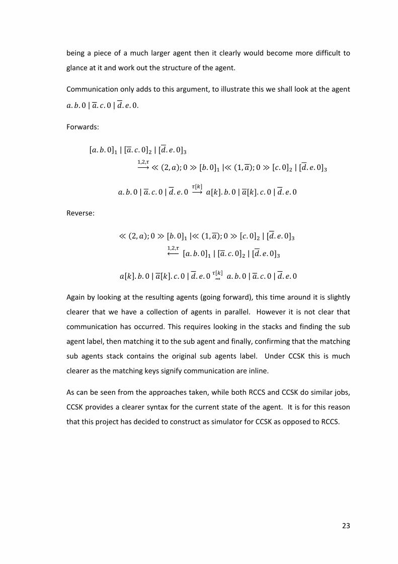
Communication only adds to this argument, to illustrate this we shall look at the agent
�. . 0 | �. �. 0 | �. %. 0.
Forwards:
[�. . 0] | [�. �. 0]� | [�. %. 0]N ,�,8>?@ ≪ �2, ��; 0 ≫ [ . 0] |≪ �1, ��; 0 ≫ [�. 0]� | [�. %. 0]N
�. . 0 | �. �. 0 | �. %. 0 8[T]>?@ �[S]. . 0 | �[S]. �. 0 | �. %. 0
Reverse:
≪ �2, ��; 0 ≫ [ . 0] |≪ �1, ��; 0 ≫ [�. 0]� | [�. %. 0]N ,�,8L?M [�. . 0] | [�. �. 0]� | [�. %. 0]N
�[S]. . 0 | �[S]. �. 0 | �. %. 0 ⇝8[T] �. . 0 | �. �. 0 | �. %. 0
Again by looking at the resulting agents (going forward), this time around it is slightly
clearer that we have a collection of agents in parallel. However it is not clear that
communication has occurred. This requires looking in the stacks and finding the sub
agent label, then matching it to the sub agent and finally, confirming that the matching
sub agents stack contains the original sub agents label. Under CCSK this is much
clearer as the matching keys signify communication are inline.
As can be seen from the approaches taken, while both RCCS and CCSK do similar jobs,
CCSK provides a clearer syntax for the current state of the agent. It is for this reason
that this project has decided to construct as simulator for CCSK as opposed to RCCS.

24
2.5 Conclusions
Over the course of this chapter, we looked at the concepts and constructs of CCS,
RCCS and CCSK complete with the SOS rules for both CCS and CCSK. We then
discussed the similarity and differences between RCCS and CCSK and while they both
do similar jobs in facilitating a reversible version of CCS, we saw CCSK had a clearer
syntax when compared with RCCS which allowed easier identification of the agents
structure. It was due to this clear syntax that lead to the decision to design and
construct a simulator based on CCSK as opposed to RCCS.

25
Chapter 3
Design
In this chapter, we shall look at some of the design requirements of the project as well
as the concept behind our internal data structure before moving on to discuss
implementation language choices. We finish this chapter with a brief feature
comparison of SimCCSK with Concurrency Workbench of New Century and FDR2 and
look at the concept design for the graphical user interface.
3.1 Requirements
We shall now look at the requirements of the system using WinSimCCSK as it is a
superset of the SimCCSK requirements (SimCCSK does not have the graphical aspects,
the Automatic Simulation feature nor the Agent Editor). We shall do this using a
system based on a technique by Tom Gilb (14) and specify the requirements as either
Functional (F) or Quality (Q). We explain the Quality requirements in further detail in
Section 3.1.1.
WinSimCCSK (F)
Agents (F) Simulation of agents.
FowardMove (F) Ability to make a forward move.
ReverseMove (F) Ability to make a reverse move.
AutomaticSim (F) Ability to automatically generate a graphical
representation of the loaded agent, to a specified
maximum depth.

26
Speed (Q) Speed of automatic simulation.
UI (F) User interface to interact with agent.
CurrentState (F) Shows current state of agent.
PreviousStates (F) Shows previous states, agent history.
GraphicalRepresentation (F) Show a graphical representation of
movement through states of the agent.
EaseOfUse (Q) Ease of tool.
SuitabilityOfLayout (Q) Suitability of data layout.
Peformance (Q) Performance of tool.
AgentEditor (F) Simple built-in text editor for agent creation / editing.
Load (F) Ability to load a pre-created agent(s) from a file.
Save (F) Ability to save agent(s) to a file for future use.
LoadToSim (F) Load defined agent(s) to simulator.
3.1.1 Quality Requirement Details
WinSimCCSK.AutomaticSim.Speed
Speed of the Automatic Simulation feature is measured by the duration of time taken
for it to complete. There is an obvious difficulty in measurement here as the duration
of time taken is clearly linked to the complexity of the agent being simulated. As such
we will base this on two measurements, one of relatively small examples which we
aim to complete in a time frame of minutes (for use in a 'live' teaching scenario) and
one of hours for slightly more complex ones (for use in one-off visualisations to be
completed in advance, possibly overnight).
WinSimCCSK.UI.EaseOfUse
WinSimCCSK is designed as a teaching tool for students. Our aim is to keep the tool
easy to use so that the focus is on the learning process calculi as opposed to learning a
tool. As ease of use is difficult to quantify, we will measure this based on student
feedback.
27
WinSimCCSK.UI.EaseOfUse.SuitabilityOfLayout
Following on from EaseOfUse, the suitability of the layout is clearly a key component
in achieving this. We aim to provide the relevant information in a logical and well laid
out fashion. Again as this is difficult to quantify, we will measure this based on student
feedback.
WinSimCCSK.UI.Performance
Performance of WinSimCCSK in interactive mode. The performance of the tool is a key
component of whether it succeeds in its aim, if the tool is too slow, it acts as an
artificial barrier to learning. We aim that in the standard interactive mode of the
simulator that all moves are completed almost instantaneously and certainly within a
few seconds.
These requirements both functional and quality provide a conceptual snapshot of
what the system should ideally achieve, look and feel like. Over the rest of this
chapter we shall look into some of the design concepts and decisions involved in
attempting to transform these requirements from a conceptual snapshot in to a
working prototype like system.
3.2 Concept
The design of any piece of software is important as it will guide the entire
development process. In this section we will look at the design concepts of SimCCSK
and some of the motivation and reasoning behind them.
By looking at the rules structures and concepts of CCSK it is apparent that there are
two key components: actions and agents. On further inspection one can observe that
actions are always embedded in agents, however it does not follow that agents must
have embedded actions. Neither does it follow that the action has or needs any
knowledge of the agent it is embedded in. This gives the situation illustrated below.
Due to the nature of the project, being to create a
component springs to mind, that being the simulator
would simulate CCSK agents
the simulator
add this concept of a simulator component into our previous illustration to generate
the following.
These three components
we saw earlier CCSK (and indeed CCS as well) does
has several ran
and Parallel agents which in
agent types exist they all share a common sense of being
example with the Choice or Parallel agent, which connects two agents together
however it does not require a specific
type. So this leads us to the following hierarchal concept of a CCSK agent.
Action
Zero
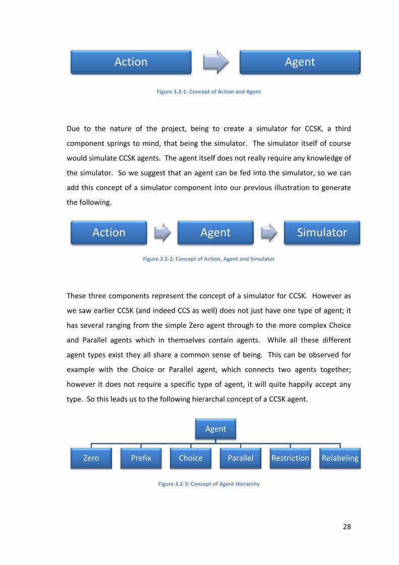
Figure 3.2-1: Concept of Action and Agent
Due to the nature of the project, being to create a
component springs to mind, that being the simulator
would simulate CCSK agents. The agent itself does not really require
the simulator. So we suggest that an agent can be fed i
concept of a simulator component into our previous illustration to generate
the following.
Figure 3.2-2: Concept of Action, Agent and Simulator
These three components represent the concept of a simulator for CCSK
we saw earlier CCSK (and indeed CCS as well) does
has several ranging from the simple Zero agent
and Parallel agents which in themselves contain agents
agent types exist they all share a common sense of being
example with the Choice or Parallel agent, which connects two agents together
however it does not require a specific type of agent, it will quite happily accept any
So this leads us to the following hierarchal concept of a CCSK agent.
Figure 3.2-3: Concept of Agent Hierarchy
Action
Action Agent
Prefix Choice
: Concept of Action and Agent
Due to the nature of the project, being to create a simulator for CCSK
component springs to mind, that being the simulator. The simulator itself of course
The agent itself does not really require any knowledge of
So we suggest that an agent can be fed into the simulator, so we can
concept of a simulator component into our previous illustration to generate
: Concept of Action, Agent and Simulator
represent the concept of a simulator for CCSK
we saw earlier CCSK (and indeed CCS as well) does not just have one type of agent;
ging from the simple Zero agent through to the more complex Choice
themselves contain agents. While all these different
agent types exist they all share a common sense of being. This can be observed for
example with the Choice or Parallel agent, which connects two agents together
type of agent, it will quite happily accept any
So this leads us to the following hierarchal concept of a CCSK agent.
: Concept of Agent Hierarchy
Agent
Agent Simulator
Agent
Choice Parallel Restriction
28
simulator for CCSK, a third
The simulator itself of course
any knowledge of
nto the simulator, so we can
concept of a simulator component into our previous illustration to generate
represent the concept of a simulator for CCSK. However as
not just have one type of agent; it
through to the more complex Choice
While all these different
This can be observed for
example with the Choice or Parallel agent, which connects two agents together;
type of agent, it will quite happily accept any
So this leads us to the following hierarchal concept of a CCSK agent.
Agent
Simulator
Restriction Relabeling
Given these two
see that the
possibly inherited
general notion of objects that could be implied from the three key components
Now that we hav
shall now give it some more thought and look at whether or not it really would be a
possible and suitable design approach
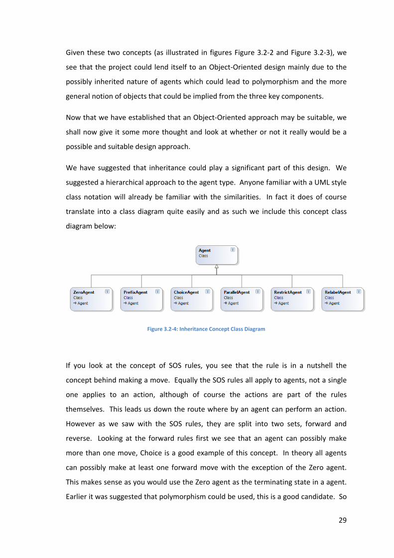
We have suggested that inheritance could play a significant part
suggested a hierarchical approach to the agent type
class notation will already be familiar with the similarities
translate in
diagram below:
If you look at the concept of SOS rules, you see that the rule is in a nutshell the
concept behind making a move
one applies to an action, although of course the actions are part of the rules
themselves
However as we saw with t
reverse. Looking at the forward rules first
more than one move
can possibly make at least one
This makes sense as
Earlier it was suggested that polymorphism could be used, this is a good candidate
Given these two concepts (as illustrated in figures
the project could lend itself to an Object
inherited nature of agents which could lead to polymorphism
general notion of objects that could be implied from the three key components
Now that we have established that an Object
shall now give it some more thought and look at whether or not it really would be a
possible and suitable design approach.
We have suggested that inheritance could play a significant part
suggested a hierarchical approach to the agent type
class notation will already be familiar with the similarities
translate into a class diagram quite easily
diagram below:
Figure 3.2-4: Inheritance Concept Class Diagram
If you look at the concept of SOS rules, you see that the rule is in a nutshell the
concept behind making a move. Equally the SOS rules all apply to agents, not a single
one applies to an action, although of course the actions are part of the rules
themselves. This leads us down the route where by an agent can perform an action
However as we saw with the SOS rules
Looking at the forward rules first
more than one move, Choice is a good example of this concept
can possibly make at least one forward
makes sense as you would use the Zero
Earlier it was suggested that polymorphism could be used, this is a good candidate
concepts (as illustrated in figures Figure 3.2-2 and Figure
project could lend itself to an Object-Oriented design mainly due to the
of agents which could lead to polymorphism
general notion of objects that could be implied from the three key components
e established that an Object-Oriented approach may be suitable, we
shall now give it some more thought and look at whether or not it really would be a
We have suggested that inheritance could play a significant part of this design
suggested a hierarchical approach to the agent type. Anyone familiar with a UML style
class notation will already be familiar with the similarities. In fact it does of course
to a class diagram quite easily and as such we include this concept class
: Inheritance Concept Class Diagram
If you look at the concept of SOS rules, you see that the rule is in a nutshell the
Equally the SOS rules all apply to agents, not a single
one applies to an action, although of course the actions are part of the rules
This leads us down the route where by an agent can perform an action
he SOS rules, they are split into two sets, forward and
Looking at the forward rules first we see that an agent can po
, Choice is a good example of this concept. In theory all agents
forward move with the exception of the Zero agent
Zero agent as the terminating state in a agent
Earlier it was suggested that polymorphism could be used, this is a good candidate
29
Figure 3.2-3), we
esign mainly due to the
of agents which could lead to polymorphism and the more
general notion of objects that could be implied from the three key components.
Oriented approach may be suitable, we
shall now give it some more thought and look at whether or not it really would be a
of this design. We
Anyone familiar with a UML style
it does of course
include this concept class
If you look at the concept of SOS rules, you see that the rule is in a nutshell the
Equally the SOS rules all apply to agents, not a single
one applies to an action, although of course the actions are part of the rules
This leads us down the route where by an agent can perform an action.
to two sets, forward and
can possibly make
In theory all agents
with the exception of the Zero agent.
the terminating state in a agent.
Earlier it was suggested that polymorphism could be used, this is a good candidate. So
we can add the default MakeMove() method t
override it in
Adding the
Looking at the reverse moves, we clearly have something similar
generally we have at least one reverse move
can get to a state going forwards there will always be a reverse move undoing the last
forward one returning you to the previous agent
polymorphic method for reverse moves (called MakePrevMove() in WinSimCCSK)
However this also gives us our first candidate for an inherited member, that being the
one for the previous agent
agent which clearly would not have a previous agent
using a null previous agent
inherited member
we can add the default MakeMove() method t
override it in a derived class to take into account of the SOS rules for the agent's type
Adding the method to our diagram gives us
Figure 3.2-5: Inheritance Concept Class Diagram (Part 2)
Looking at the reverse moves, we clearly have something similar
generally we have at least one reverse move
can get to a state going forwards there will always be a reverse move undoing the last
forward one returning you to the previous agent
polymorphic method for reverse moves (called MakePrevMove() in WinSimCCSK)
However this also gives us our first candidate for an inherited member, that being the
one for the previous agent. There is of course an exception to this, that being the f
agent which clearly would not have a previous agent
using a null previous agent for the first, thus not impacting on
inherited member. By adding these two additions we get the following:
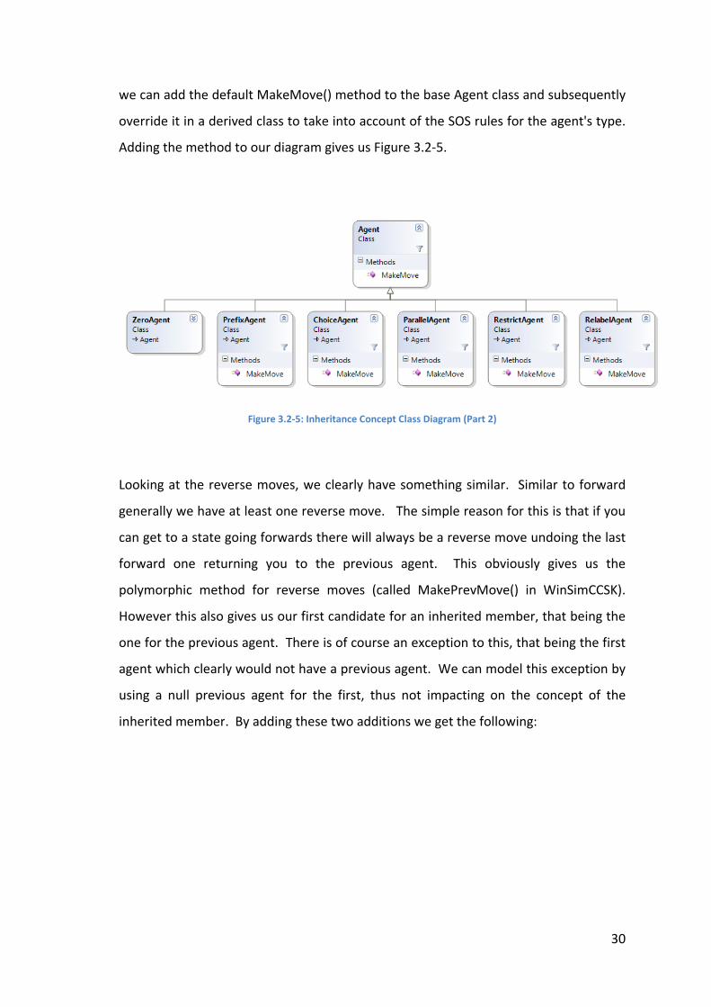
we can add the default MakeMove() method to the base Agent class and subsequently
derived class to take into account of the SOS rules for the agent's type
method to our diagram gives us Figure 3.2-5.
: Inheritance Concept Class Diagram (Part 2)
Looking at the reverse moves, we clearly have something similar. Similar to
generally we have at least one reverse move. The simple reason for this is that if you
can get to a state going forwards there will always be a reverse move undoing the last
forward one returning you to the previous agent. This obviously gives u
polymorphic method for reverse moves (called MakePrevMove() in WinSimCCSK)
However this also gives us our first candidate for an inherited member, that being the
There is of course an exception to this, that being the f
agent which clearly would not have a previous agent. We can model this exception by
for the first, thus not impacting on the concept of the
By adding these two additions we get the following:
30
o the base Agent class and subsequently
derived class to take into account of the SOS rules for the agent's type.
Similar to forward
The simple reason for this is that if you
can get to a state going forwards there will always be a reverse move undoing the last
This obviously gives us the
polymorphic method for reverse moves (called MakePrevMove() in WinSimCCSK).
However this also gives us our first candidate for an inherited member, that being the
There is of course an exception to this, that being the first
We can model this exception by
the concept of the
By adding these two additions we get the following:
We have seen that an Object
with being a highly suitable approach to take
use of both polymorphism
along with the use of inheritance for the shared concept of a predecessor
shown this
interaction of the software
3.3 Internal Data Structures
In our initial concept, we came to the conclusion that agents are linked to other agents
and that actions would somehow let us move between agents
the agent that . 0 links to the Zero agent, this would suggest a design looking something like
this:
a.b.0
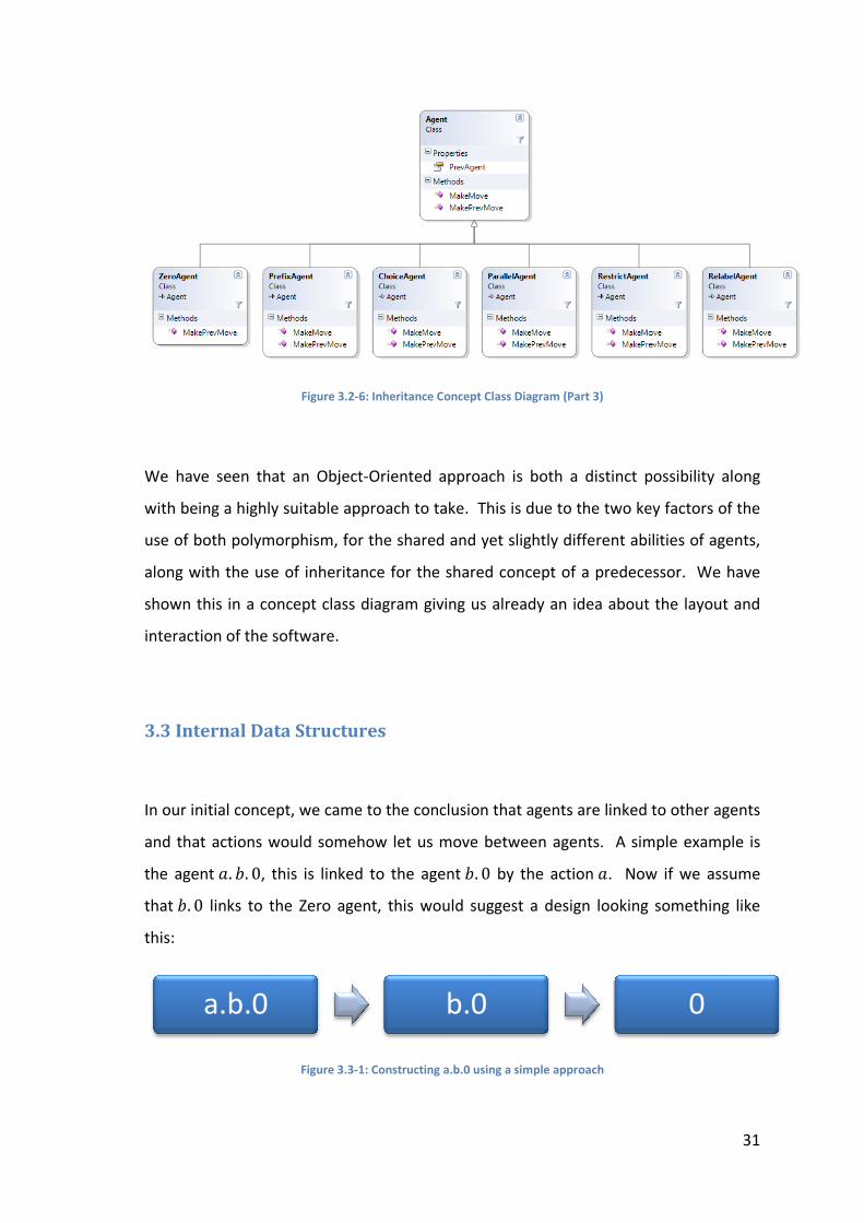
Figure 3.2-6: Inheritance Concept Class Diagram (Part 3
e have seen that an Object-Oriented approach is both a distinct possibility along
with being a highly suitable approach to take
use of both polymorphism, for the shared and yet slightly different abilities of agents
along with the use of inheritance for the shared concept of a predecessor
this in a concept class diagram giving us
interaction of the software.
Internal Data Structures
In our initial concept, we came to the conclusion that agents are linked to other agents
and that actions would somehow let us move between agents
�. . 0, this is linked to the agent
links to the Zero agent, this would suggest a design looking something like
Figure 3.3-1: Constructing a.b.0 using a simple approach
a.b.0
ce Concept Class Diagram (Part 3)
Oriented approach is both a distinct possibility along
with being a highly suitable approach to take. This is due to the two key factors
for the shared and yet slightly different abilities of agents
along with the use of inheritance for the shared concept of a predecessor
in a concept class diagram giving us already an idea about the layout and
In our initial concept, we came to the conclusion that agents are linked to other agents
and that actions would somehow let us move between agents. A simple exam
, this is linked to the agent . 0 by the action �. Now if we assume
links to the Zero agent, this would suggest a design looking something like
ructing a.b.0 using a simple approach
b.0
31
Oriented approach is both a distinct possibility along
due to the two key factors of the
for the shared and yet slightly different abilities of agents,
along with the use of inheritance for the shared concept of a predecessor. We have
already an idea about the layout and
In our initial concept, we came to the conclusion that agents are linked to other agents
A simple example is
Now if we assume
links to the Zero agent, this would suggest a design looking something like
0

This seems a perfectly reasonable and intuitive approach to take, however it would
seem to be duplicating data, if we take a look at
of . 0 and the Zero agent embedded in the original agent and therefore the
subsequent copies are not ideal
looking at such simple agents this
�. . 0 + �.
While it holds all the information, we still have the duplication, however we now ha
two branches of duplicated data, imagine what we would end up with if we had
multiple choices.
It is clear that this is not going to be the most efficient way forward however parts of
the concept do in fact have their uses
of a tree like structure, similar derivations can be made for other constructs in CCSK
Given this we suggest that we can base the internal repre
abstract syntax tree.
If we now apply the concept of an abstract syntax tree (AST), we can break down our
two examples above as follows:
�.
�.
a.b.0 + c.d.0
This seems a perfectly reasonable and intuitive approach to take, however it would
seem to be duplicating data, if we take a look at
and the Zero agent embedded in the original agent and therefore the
subsequent copies are not ideal. Although we could probably get away with this when
looking at such simple agents this clearly is not very scalable, if we consider agent
. �. 0, we would end up with something looking similar to this:
Figure 3.3-2: Constructing a.b.0 + c.d.0 using a simple approach
While it holds all the information, we still have the duplication, however we now ha
two branches of duplicated data, imagine what we would end up with if we had
multiple choices.
It is clear that this is not going to be the most efficient way forward however parts of
the concept do in fact have their uses. If we look at
of a tree like structure, similar derivations can be made for other constructs in CCSK
Given this we suggest that we can base the internal repre
abstract syntax tree.
If we now apply the concept of an abstract syntax tree (AST), we can break down our
two examples above as follows:
. 0 is Prefix(�, . 0) with action
similarly.
. 0 + �. �. 0 is Choice(�. . 0 These two sub-trees can be derived as above
a.b.0 + c.d.0a.b.0
c.d.0
This seems a perfectly reasonable and intuitive approach to take, however it would
seem to be duplicating data, if we take a look at �. . 0, we can clearly see the data
and the Zero agent embedded in the original agent and therefore the
Although we could probably get away with this when
clearly is not very scalable, if we consider agent
we would end up with something looking similar to this:
: Constructing a.b.0 + c.d.0 using a simple approach
While it holds all the information, we still have the duplication, however we now ha
two branches of duplicated data, imagine what we would end up with if we had
It is clear that this is not going to be the most efficient way forward however parts of
If we look at Figure 3.3-2 we can see the start
of a tree like structure, similar derivations can be made for other constructs in CCSK
Given this we suggest that we can base the internal representation of agents using an
If we now apply the concept of an abstract syntax tree (AST), we can break down our
) with action � and sub-tree . 0. . 0 can be derived
0, �. �. 0) with sub-trees �. trees can be derived as above.
a.b.0 b.0
c.d.0 d.0
32
This seems a perfectly reasonable and intuitive approach to take, however it would
, we can clearly see the data
and the Zero agent embedded in the original agent and therefore the
Although we could probably get away with this when
clearly is not very scalable, if we consider agent
we would end up with something looking similar to this:
While it holds all the information, we still have the duplication, however we now have
two branches of duplicated data, imagine what we would end up with if we had
It is clear that this is not going to be the most efficient way forward however parts of
we can see the start
of a tree like structure, similar derivations can be made for other constructs in CCSK.
sentation of agents using an
If we now apply the concept of an abstract syntax tree (AST), we can break down our
can be derived
. 0 and �. �. 0.
0
0

33
More generally, we can see this approach being applied to the constructs of CCSK as
shown below.
�. / is Prefix(�, /) with action � and sub-tree /.
/ + 4 is Choice with sub-trees / and 4.
/ | 4 is Parallel Composition with sub-trees / and 4.
/\� is Restriction with sub-tree / being restricted by the set of actions �.
/[-] is Relabeling with sub-tree / being relabelled according to function -.
As we can see, these five definitions already give us a clear approach to a design for
WinSimCCSK. They show how each agent can be defined using a combination of sub-
trees and additional information to allow us to model the various aspects of CCSK.
Earlier we suggested the possibly polymorphic methods of MakeMove() and
MakePrevMove(). The AST approach supports this notion with a move being able to
be made in a similar fashion to the SOS rules whereby the move is made if the move
can be made by a component of the agent (or sub-tree of the AST in this case).
3.4 Implementation Language
Usually the process of deciding the implementation language is guided by three key
technical factors. The three technical factors are:
1) the suitability of the language to the task in hand
2) the possible reuse of existing code either via existing libraries of functions
which could either be custom written or more globally available APIs such
as .NET or the Java API
3) the target platform(s) of the project.
Over this section we will look at these factors and how they can guide the choices of
the SimCCSK project.

34
The suitability of a language to the task in hand is one of the most important factors
which could make or break any software project. On the simplest level it is about
choosing a language that matches the design concept. A programming language
should always be chosen such that its coding paradigm (e.g. object oriented,
functional, etc) matches that of the design paradigm. If we look at the SimCCSK
project, we saw previously that the concept lent itself to an Object-Oriented approach.
Of course there are several such languages, in fact Wikipedia lists over 100 different
Object-Oriented languages or variants (15). It would be impractical to look at all of
them here so for the rest of this discussion we shall look at C++, C#, Java and Visual
Basic.
The target platform(s) of any project can often be crucial in guiding design choice.
Depending on the project this could already be fixed or nearly fixed, for example a
video game would be designed to work on a console of some sort, either a home
based one such as the Xbox 360 or PlayStation 3 or a handheld one such as the
Nintendo DS or PlayStation Portable. Most projects target platform however would be
a desktop workstation PC, whilst this in itself is a decision, it raises a secondary
decision. A PC by itself, whilst a platform, is not defined enough from a development
perspective. Specifically a PC's platform is more usually described by either it’s
operating system such as Windows Vista or Mac OS X 10.5 “Leopard” or family of
operating systems such as Win32 or Mac OS X. From this point, the project’s platform
can be chosen based on a target audience or a gap in the market. Examples of this are
that most businesses use some variety of Windows so it is no surprise that a number
of Office applications are designed for use on the Windows platform. Equally the
world of the Mac is most often used by more creative people such as artists, musicians
and film or sound editors, so equally such products are designed for the Mac platform,
although a number also do have Windows counterparts. In the case of SimCCSK we do
not really have either of these guiding our process as the project is more about a
prototype than a commercial level software production. For this reason, along with
the fact that most (if not all) universities will provide access to Windows PCs and the
fact that all of the languages run on Windows, it would seem an appropriate decision
to choose Windows as the platform as this does not limit our language options.

35
Choosing a non Windows platform would of course remove C# and Visual Basic as the
.NET framework is not common place on other platforms and therefore could not be
relied on.
The use of existing libraries is clearly becoming more common place. The simple
reason that if everything was always written from the ground up, any software project
would take far longer and be more expensive to produce. This is, of course, fairly
obvious as for example at the beginning of any project the design team would spend
time recreating code they had previously used for the new project. A library is a
solution to this very issue. In the modern world APIs and standard libraries are more
common due to the fact that a very large number of software projects are based
around similar ideas at some point, whether it is that they use something as simple as
a String or a slightly more complex structure such as a linked-list there are a number of
key small components that make up these projects. As such most modern
programming languages have some form of standard library or API to deal with this
frequently used boilerplate type code. Our four languages are no exception to this,
C++ has the Standard Library (16) and the Standard Template Library (17), also should
the decision be made to write the software for a Win32 or Win64 platform the .NET
Framework (18) (19) and associated libraries would also be an option. C# and Visual
Basic both have access to the .NET Framework and Java has the Java API which is
contained within the Java Platforms of which there are three, Java ME (Micro Edition)
for environments with limited resources; Java SE (Standard Edition) for standard
workstation environments and Java EE (Enterprise Edition) for distributed
environments and the internet. For our purposes we are interested in Java SE (20)
(21) and for the rest of the discussion we use Java and the Java SE platform
interchangeably.
Apart from the very general language ‘standard’ APIs, other APIs or libraries can come
in to play. One of our requirements for the GUI version was the ability to see a
graphical representation. All four of the languages have some form of graphical
drawing ability, .NET (so by extension C#, C++ and Visual Basic) and C++ (natively
under Windows) have the ability to draw via GDI+ (22) (23), Java in order to maintain
its cross platform nature uses Swing, however Swing results in Java based GUIs looking

36
different to their more native counterparts. An extension to graphical drawing is of
course hardware accelerated graphics; again all four languages have some form of
hardware accelerated graphics. C++ has DirectX (24) (25), which allows native based
2D and 3D hardware accelerated graphics. .NET languages have a couple of options,
managed DirectX or XNA (26) (27) which is a superseding (and natural successor) of
managed DirectX. XNA is officially only supported by C# currently however being .NET
based it can technically be used by any .NET language. Java has the community based
project of Java3D, which whilst is not quite hardware accelerated in the same sense as
DirectX or XNA due to Java’s cross platform nature, there is some hardware
acceleration options available to it. Finally another option is a ‘plug-in’ style libraries
for graph drawing, such as Microsoft Automatic Graph Layout (MSAGL) (28) (29) which
is a project by Lev Nachmanson at Microsoft Research (Redmond) which allows graphs
to be created and viewed using a .NET enabled language. Based on these observations
and to allow the project to move in one of a number of directions, C# seems a suitable
choice for the implementation language of SimCCSK as it allows the possible use of
GDI+, DirectX, XNA or MSAGL.
3.5 Related Work
3.5.1 CWB-NC
Concurrency Workbench of the New Century (CWB-NC) (30) (31) (32) is one of the
leading tools currently used for the simulation of CCS and similar process calculi
created using SML of New Jersey by Rance Cleaveland, Steve Sims and Tan Li with its
original release in 1996 through to its current version 1.2 released in 2000. CWB-NC is
primarily text based although there is a GUI available which uses Expectk. The system
allows for simulations of agents; however this is very much a unidirectional process,
yet this does allow the production of a trace of an agent.

37
Concurrency Workbench has the capabilities to work with multiple process calculi
mainly CCS and derivatives of it such as Prioritized CCS, Timed CCS and Synchronous
CCS, along with Communicating Sequential Processes (CSP) and Basic LOTOS. Along
with its simulation ability, it also has the ability to do bisimulation, model checking and
equivalence checking.
3.5.2 FDR2
FDR2 (33) is refinement and model checker for CSP (34) (35). It is a commercial
product created by Formal Systems (Europe) Ltd, which was formed in 1989 by some
of the Oxford University Computing Laboratory and some of the founders of its sister
company Formal Systems Design and Development Inc.
FDR2 functionality revolves around its two key functions of refinement and model
checking for CSP; it is a GUI based application however it lacks any graphical
representation of the system being looked at.
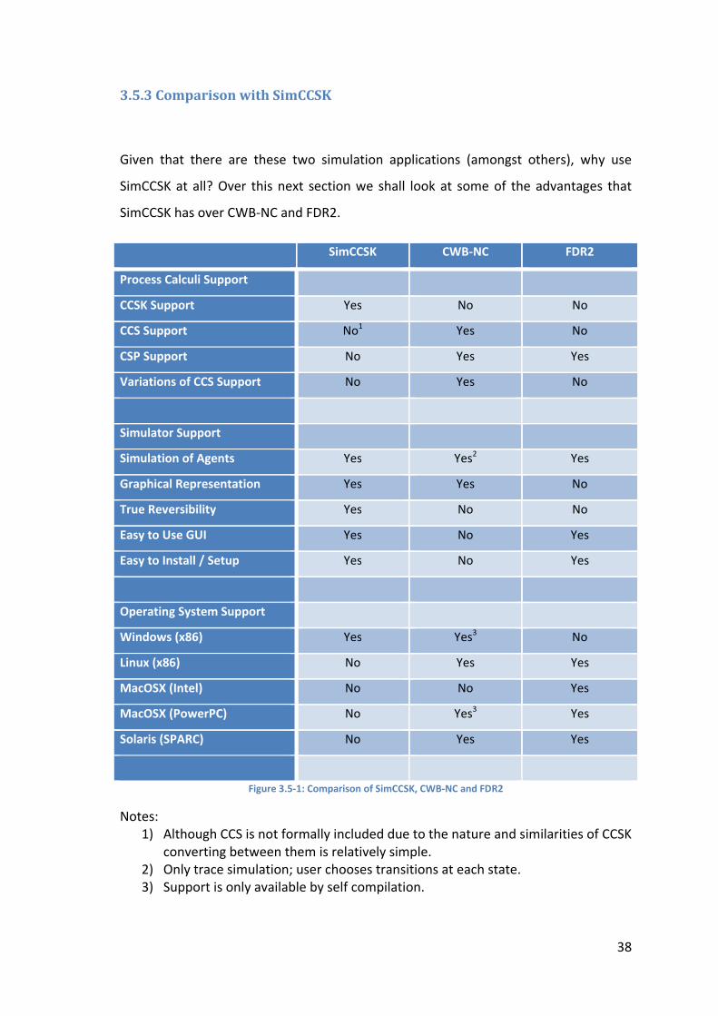
38
3.5.3 Comparison with SimCCSK
Given that there are these two simulation applications (amongst others), why use
SimCCSK at all? Over this next section we shall look at some of the advantages that
SimCCSK has over CWB-NC and FDR2.
SimCCSK CWB-NC FDR2
Process Calculi Support
CCSK Support Yes No No
CCS Support No1 Yes No
CSP Support No Yes Yes
Variations of CCS Support No Yes No
Simulator Support
Simulation of Agents Yes Yes2 Yes
Graphical Representation Yes Yes No
True Reversibility Yes No No
Easy to Use GUI Yes No Yes
Easy to Install / Setup Yes No Yes
Operating System Support
Windows (x86) Yes Yes3
No
Linux (x86) No Yes Yes
MacOSX (Intel) No No Yes
MacOSX (PowerPC) No Yes3 Yes
Solaris (SPARC) No Yes Yes
Figure 3.5-1: Comparison of SimCCSK, CWB-NC and FDR2
Notes:
1) Although CCS is not formally included due to the nature and similarities of CCSK
converting between them is relatively simple.
2) Only trace simulation; user chooses transitions at each state.
3) Support is only available by self compilation.

39
Here we see that while SimCCSK does not have all the support of either Concurrency
Workbench or FDR2, we can see that SimCCSK achieves its goals and is (out of the
three) the only one to handle true reversibility, which means that it is the only one out
of the three which can handle going backwards within the calculi. This is particularly
prevalent in comparing Concurrency Workbench trace visualisation with
WinSimCCSK’s graph representation. In terms of language compatibility it is clear that
Concurrency Workbench is the most appropriate in terms of the number of languages
supported, however while FDR and SimCCSK only support the one language, SimCCSK
is currently the only simulator to support CCSK. Equally while Concurrency Workbench
and FDR2 have additional functionality such as model checking, it is worth
remembering that the purpose of the SimCCSK project was to produce a simulator.
Additionally both Concurrency Workbench and FDR2 have been around far longer and
usually more functionality is added in later versions. Also it is worth noting that FDR2
does not have any form of graphical visualisation of the model (although does run in a
GUI) which is something that SimCCSK has.
Finally a couple of the key points of the SimCCSK project is to create a simulator that is
both simple to install along with being easy and intuitive to use. Out of the three,
SimCCSK is the simplest to install as it is packaged in one file that just need to be
unpacked (however it does require the .NET library to be installed, this is common
place on most copies of Windows, so this has been discounted from this discussion).
FDR2 comes a very close second, again being in packaged in one file that needs to be
unpacked, it then requires a second small step of creating an environment variable for
it before it can be run. Concurrency Workbench however is not the easiest by far,
while the instructions are clear, usually it is often easiest to self compile (which
requires SML of New Jersey) with whatever version of the libraries you happen to be
using. This is of importance if you wish to use the GUI as Concurrency Workbence
requires Expectk (version 5.20, current version 5.43), which in turn requires Tcl
(version 7.5, current version 8.5) and Tk (version 4.1, current version 8.5). Based on
personal experience Concurrency Workbench seems to have an issue working with the
current versions, meaning that it is often easier to download and use the older
versions its expecting, however this means you may end up with both the older
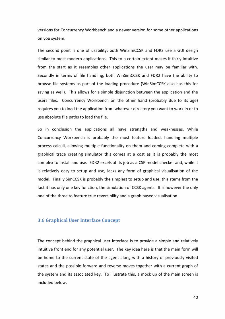
40
versions for Concurrency Workbench and a newer version for some other applications
on you system.
The second point is one of usability; both WinSimCCSK and FDR2 use a GUI design
similar to most modern applications. This to a certain extent makes it fairly intuitive
from the start as it resembles other applications the user may be familiar with.
Secondly in terms of file handling, both WinSimCCSK and FDR2 have the ability to
browse file systems as part of the loading procedure (WinSimCCSK also has this for
saving as well). This allows for a simple disjunction between the application and the
users files. Concurrency Workbench on the other hand (probably due to its age)
requires you to load the application from whatever directory you want to work in or to
use absolute file paths to load the file.
So in conclusion the applications all have strengths and weaknesses. While
Concurrency Workbench is probably the most feature loaded, handling multiple
process calculi, allowing multiple functionality on them and coming complete with a
graphical trace creating simulator this comes at a cost as it is probably the most
complex to install and use. FDR2 excels at its job as a CSP model checker and, while it
is relatively easy to setup and use, lacks any form of graphical visualisation of the
model. Finally SimCCSK is probably the simplest to setup and use, this stems from the
fact it has only one key function, the simulation of CCSK agents. It is however the only
one of the three to feature true reversibility and a graph based visualisation.
3.6 Graphical User Interface Concept
The concept behind the graphical user interface is to provide a simple and relatively
intuitive front end for any potential user. The key idea here is that the main form will
be home to the current state of the agent along with a history of previously visited
states and the possible forward and reverse moves together with a current graph of
the system and its associated key. To illustrate this, a mock up of the main screen is
included below.
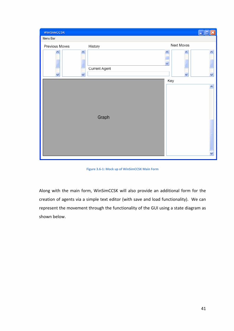
Along with the main form, WinSimCCSK will also provid
creation of agents via a simple text editor (with save and load functionality)
represent the movement through the functionality of the GUI using a state diagram as
shown below.
Figure 3.6-1: Mock up of WinSimCCSK Main Form
Along with the main form, WinSimCCSK will also provid
creation of agents via a simple text editor (with save and load functionality)
represent the movement through the functionality of the GUI using a state diagram as
shown below.
Mock up of WinSimCCSK Main Form
Along with the main form, WinSimCCSK will also provide an additional form for the
creation of agents via a simple text editor (with save and load functionality)
represent the movement through the functionality of the GUI using a state diagram as
41
e an additional form for the
creation of agents via a simple text editor (with save and load functionality). We can
represent the movement through the functionality of the GUI using a state diagram as

42
Figure 3.6-2: GUI State Diagram
3.7 Conclusions
Over the course of the chapter, we have looked at the concepts behind a CCSK
simulator and its required components along with the theoretical links between them
and how this would seem to suit an Object-Oriented approach. We have seen how we
can take these concepts and derive a concept of a possible and feasible internal data
structure. Finally we discussed an approach to choosing an implementation language
and then used this approach to look at SimCCSK and chose C# as the implementation
language based on the different factors involved with this project.

43
Chapter 4
Implementation
In this chapter we shall look into some of the implementation details of the project
including the construction of the internal data structure before moving on to look at
the construction and workings of SimCCSK, the console based simulator.
4.1 Laying the Ground Work
As discussed in Chapter 3, SimCCSK is designed to use an Object-Oriented approach
due to the possibility of inherited attributes and polymorphism for the agent
components. We then went on to show a concept class diagram for the inheritance of
agents (Figure 3.2-6). From this concept diagram, we can easily add the two additional
components we have identified, being the Action and the Simulator. This is shown in
Figure 4.1-1 below.
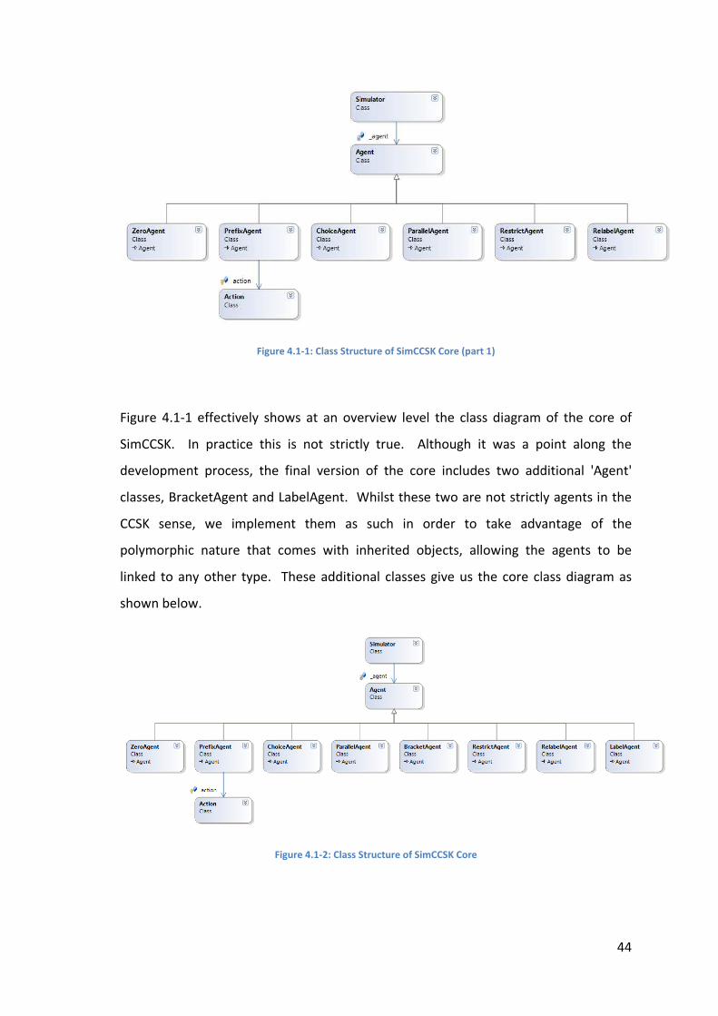
Figure 4.1
SimCCSK.
development process, the final version of the core includes two additional 'Agent'
classes, BracketAgent and LabelAgent
CCSK sense, we implement them as such in order to take advantage of the
polymorphic nature
linked to any other type
shown below.
Figure 4.1-1: Class Structure of SimCCSK
-1 effectively shows at an overview level the class diagram of the core of
. In practice this is not strictly true
opment process, the final version of the core includes two additional 'Agent'
classes, BracketAgent and LabelAgent. Whilst these two are not strictly agents in the
CCSK sense, we implement them as such in order to take advantage of the
polymorphic nature that comes with inherited objects, allowing the agents to be
linked to any other type. These additional
shown below.
Figure 4.1-2: Class Structure of SimCCSK Core
lass Structure of SimCCSK Core (part 1)
effectively shows at an overview level the class diagram of the core of
In practice this is not strictly true. Although it was a point along the
opment process, the final version of the core includes two additional 'Agent'
Whilst these two are not strictly agents in the
CCSK sense, we implement them as such in order to take advantage of the
that comes with inherited objects, allowing the agents to be
additional classes give us the core class diagram as
: Class Structure of SimCCSK Core
44
effectively shows at an overview level the class diagram of the core of
Although it was a point along the
opment process, the final version of the core includes two additional 'Agent'
Whilst these two are not strictly agents in the
CCSK sense, we implement them as such in order to take advantage of the
that comes with inherited objects, allowing the agents to be
classes give us the core class diagram as
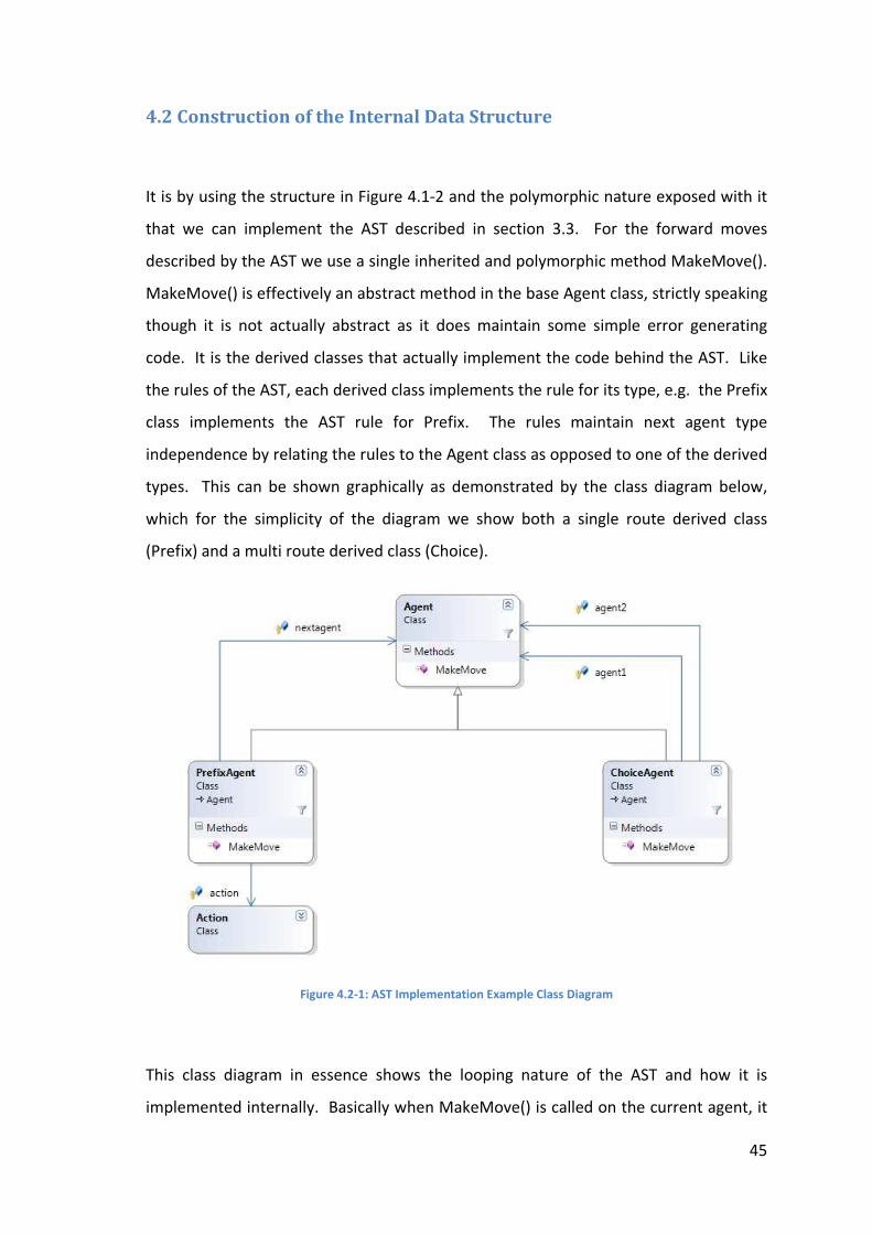
4.2 Construction of the Internal Data Structure
It is by using
that we can implement the AST de
described by the AST we use a single inherited and polymorphic method MakeMove()
MakeMove() is effectively an abstr
though it is not actually abstract as it does maintain some simple error generating
code. It is the derived classes that actually implement the code behind the AST
the rules of the AST
class implements the AST rule for Prefix
independence
types. This can be shown gra
which for the simplicity of the diagram we show both a single route derived class
(Prefix) and a multi route derived class (Choice).
This class diagram in essence shows the looping nature of the AST and how it is
implemented internally
Construction of the Internal Data Structure
It is by using the structure in Figure 4.1-2
that we can implement the AST described in section
described by the AST we use a single inherited and polymorphic method MakeMove()
MakeMove() is effectively an abstract method in the base Agent class, strictly speaking
though it is not actually abstract as it does maintain some simple error generating
It is the derived classes that actually implement the code behind the AST
the rules of the AST, each derived class implements the rule for its type, e.g
class implements the AST rule for Prefix
independence by relating the rules to the Agent class as opposed to one of the derived
This can be shown graphically as demonstrated by the class diagram below,
which for the simplicity of the diagram we show both a single route derived class
(Prefix) and a multi route derived class (Choice).
Figure 4.2-1: AST Implementation Example Class Diagram
This class diagram in essence shows the looping nature of the AST and how it is
implemented internally. Basically when MakeMove() is called on the current agent, it
Construction of the Internal Data Structure
2 and the polymorphic nature exposed
scribed in section 3.3. For the forward moves
described by the AST we use a single inherited and polymorphic method MakeMove()
act method in the base Agent class, strictly speaking
though it is not actually abstract as it does maintain some simple error generating
It is the derived classes that actually implement the code behind the AST
ived class implements the rule for its type, e.g
class implements the AST rule for Prefix. The rules maintain next agent type
by relating the rules to the Agent class as opposed to one of the derived
phically as demonstrated by the class diagram below,
which for the simplicity of the diagram we show both a single route derived class
(Prefix) and a multi route derived class (Choice).
Implementation Example Class Diagram
This class diagram in essence shows the looping nature of the AST and how it is
Basically when MakeMove() is called on the current agent, it
45
the polymorphic nature exposed with it
For the forward moves
described by the AST we use a single inherited and polymorphic method MakeMove().
act method in the base Agent class, strictly speaking
though it is not actually abstract as it does maintain some simple error generating
It is the derived classes that actually implement the code behind the AST. Like
ived class implements the rule for its type, e.g. the Prefix
The rules maintain next agent type
by relating the rules to the Agent class as opposed to one of the derived
phically as demonstrated by the class diagram below,
which for the simplicity of the diagram we show both a single route derived class
This class diagram in essence shows the looping nature of the AST and how it is
Basically when MakeMove() is called on the current agent, it
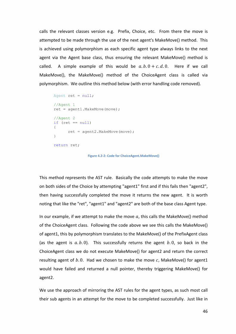
46
calls the relevant classes version e.g. Prefix, Choice, etc. From there the move is
attempted to be made through the use of the next agent's MakeMove() method. This
is achieved using polymorphism as each specific agent type always links to the next
agent via the Agent base class, thus ensuring the relevant MakeMove() method is
called. A simple example of this would be �. . 0 + �. �. 0. Here if we call
MakeMove(), the MakeMove() method of the ChoiceAgent class is called via
polymorphism. We outline this method below (with error handling code removed).
Agent ret = null;
//Agent 1
ret = agent1.MakeMove(move);
//Agent 2
if (ret == null)
{
ret = agent2.MakeMove(move);
}
return ret;
Figure 4.2-2: Code for ChoiceAgent.MakeMove()
This method represents the AST rule. Basically the code attempts to make the move
on both sides of the Choice by attempting "agent1" first and if this fails then "agent2",
then having successfully completed the move it returns the new agent. It is worth
noting that like the "ret", "agent1" and "agent2" are both of the base class Agent type.
In our example, if we attempt to make the move �, this calls the MakeMove() method
of the ChoiceAgent class. Following the code above we see this calls the MakeMove()
of agent1, this by polymorphism translates to the MakeMove() of the PrefixAgent class
(as the agent is �. . 0). This successfully returns the agent . 0, so back in the
ChoiceAgent class we do not execute MakeMove() for agent2 and return the correct
resulting agent of . 0. Had we chosen to make the move �, MakeMove() for agent1
would have failed and returned a null pointer, thereby triggering MakeMove() for
agent2.
We use the approach of mirroring the AST rules for the agent types, as such most call
their sub agents in an attempt for the move to be completed successfully. Just like in
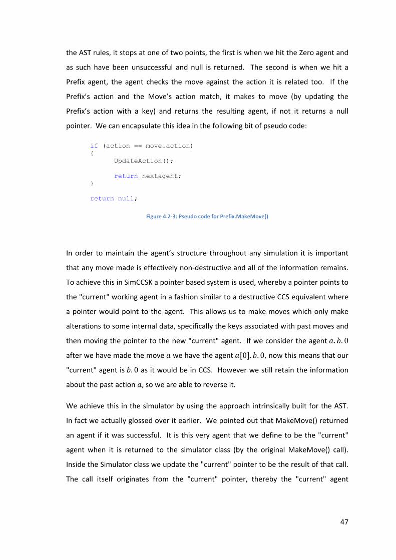
47
the AST rules, it stops at one of two points, the first is when we hit the Zero agent and
as such have been unsuccessful and null is returned. The second is when we hit a
Prefix agent, the agent checks the move against the action it is related too. If the
Prefix’s action and the Move’s action match, it makes to move (by updating the
Prefix’s action with a key) and returns the resulting agent, if not it returns a null
pointer. We can encapsulate this idea in the following bit of pseudo code:
if (action == move.action)
{
UpdateAction();
return nextagent;
}
return null;
Figure 4.2-3: Pseudo code for Prefix.MakeMove()
In order to maintain the agent’s structure throughout any simulation it is important
that any move made is effectively non-destructive and all of the information remains.
To achieve this in SimCCSK a pointer based system is used, whereby a pointer points to
the "current" working agent in a fashion similar to a destructive CCS equivalent where
a pointer would point to the agent. This allows us to make moves which only make
alterations to some internal data, specifically the keys associated with past moves and
then moving the pointer to the new "current" agent. If we consider the agent �. . 0
after we have made the move � we have the agent �[0]. . 0, now this means that our
"current" agent is . 0 as it would be in CCS. However we still retain the information
about the past action �, so we are able to reverse it.
We achieve this in the simulator by using the approach intrinsically built for the AST.
In fact we actually glossed over it earlier. We pointed out that MakeMove() returned
an agent if it was successful. It is this very agent that we define to be the "current"
agent when it is returned to the simulator class (by the original MakeMove() call).
Inside the Simulator class we update the "current" pointer to be the result of that call.
The call itself originates from the "current" pointer, thereby the "current" agent

48
returns the next "current" agent on a successful return of MakeMove(), as shown by
the line of code below.
current = current.MakeMove(move);
Figure 4.2-4: Calling MakeMove() and Updating "current" Agent
In order to maintain access to the entire agent (and by extension its current state) we
also maintain a second pointer in the Simulator class, the head of the AST, which
allows access to the current state of the agent for outputting to the user.
These two concepts combined encapsulate the functionality of MakeMove() for all
agent types. We can represent the simulator MakeMove() sequence graphical as
shown below.
Figure 4.2-5: State Diagram for MakeMove()

49
As previously stated the functionality of the AST rules are encapsulated in each
derived agents MakeMove() method. All work in a similar way, attempting to make
the move and if successful returning the new "current" agent. However there is a
subtle difference with the Parallel agent. The key reason for this is the maintaining of
its structure in a non-destructive fashion whilst retaining its parallel functionality. In
SimCCSK we achieve this by deploying a local pointer system (within the scope of the
parallel agent), on top of the global "current" agent pointer system as described
earlier.
If we look at the other agent types, they all share a destructive nature in that once the
agent has been executed it has no influence on its sub agents. Parallel is different in
that the parallel composition lives on between the sub agents. For the Parallel agent,
in order to preserve the history of the agent, we duplicate the concept of the "current"
agent at a local level. Instead of MakeMove() returning the next agent in the
sequence to become the current agent, Parallel agents return themselves in order to
continue the parallel composition across the sub agents. This however only tells half
of the story, clearly if an agent just returns itself, nothing has changed and we would
be able to make the move indefinitely without achieving anything. To solve this
problem, Parallel agents act based on their local "current" sub agents. As such
MakeMove() in a Parallel agent updates the "current" sub agents using exactly the
same approach we took for agents in general.
For reverse moves we use the method MakePrevMove() to go back up, utilising a
common inherited member "PrevAgent". PrevAgent as stated earlier always links back
to its parent agent (with the exception of the root agent, in which case it is null). For
the majority of agent types MakePrevMove() calls up the tree to check for the reverse
move and if found is returned as the new "current" agent to pass back to the
simulator, in a similar approach to MakeMove(). Parallel of course is an exception to
this, due to the introduction of the local "current" sub agents. In the case of Parallel,
MakePrevMove() utilises a similar approach on the "current" sub agents, reversing
them back up towards their initial states. Should the Parallel agent be in its original
state (i.e. all sub agents are in their original state), then Parallel calls up the tree using
the same approach as the other agent types.

50
For both forward and reverse moves, the Parallel agent type is further expanded in
order to deal with communicating moves. In the case of communicating moves, the
Parallel agent attempts to perform (or reverse) the action and its counterpart on two
distinct sub agents and only if it can achieve both does it update the two relevant
"current" sub agents. Communicating moves are distinguished from non
communicating moves by an addition prefix of "t->" for the communicating ones.
Equally communicating moves a denoted using their action as opposed to its
counterpart (overbar version).
4.3 Putting it Together
Now with the ground work and internal structure laid out, it is time to put these
together to create SimCCSK. SimCCSK is a console based, command line driven
application (although as hinted at, a graphical counterpart WinSimCCSK also exists
which will discussed in Chapter 5), based around a core setup. This core revolves
around the design of a Simulator object which processes an agent which itself is a
combination of actions and agents constructed as previously discussed. On top of this
sits the command line interface which is designed with the notion of informing the
user what state they are in and then providing the options for moves in both a forward
and reverse direction.
This is in fact the core loop of the application after loading an agent. Provided that the
execution is not halted, the simulator will continuously calculate the possible forward
and reverse moves (using a similar method to MakeMove()). Once the move lists have
been generated it provides the current state of the agent, lists the possible forward
and reverse moves to the user and then the simulator will make a move from the list
based on user input (using MakeMove()). After successful completion of the move it
updates the state of the agent and starts the loop again.
The state itself is represented using the standard CCSK representation which has been
used throughout this document. The single exception to this is that due to the
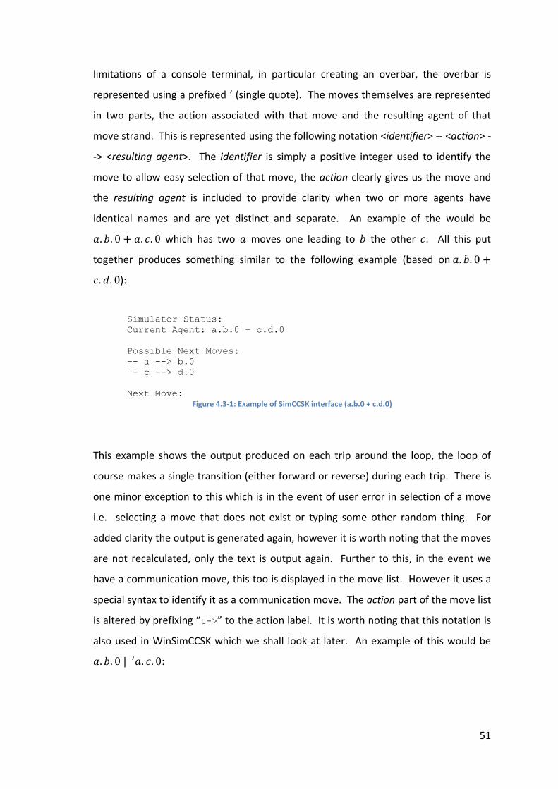
51
limitations of a console terminal, in particular creating an overbar, the overbar is
represented using a prefixed ‘ (single quote). The moves themselves are represented
in two parts, the action associated with that move and the resulting agent of that
move strand. This is represented using the following notation <identifier> -- <action> -
-> <resulting agent>. The identifier is simply a positive integer used to identify the
move to allow easy selection of that move, the action clearly gives us the move and
the resulting agent is included to provide clarity when two or more agents have
identical names and are yet distinct and separate. An example of the would be
�. . 0 + �. �. 0 which has two � moves one leading to the other �. All this put
together produces something similar to the following example (based on �. . 0 +�. �. 0):
Simulator Status:
Current Agent: a.b.0 + c.d.0
Possible Next Moves:
–- a --> b.0
–- c --> d.0
Next Move:
Figure 4.3-1: Example of SimCCSK interface (a.b.0 + c.d.0)
This example shows the output produced on each trip around the loop, the loop of
course makes a single transition (either forward or reverse) during each trip. There is
one minor exception to this which is in the event of user error in selection of a move
i.e. selecting a move that does not exist or typing some other random thing. For
added clarity the output is generated again, however it is worth noting that the moves
are not recalculated, only the text is output again. Further to this, in the event we
have a communication move, this too is displayed in the move list. However it uses a
special syntax to identify it as a communication move. The action part of the move list
is altered by prefixing “t->” to the action label. It is worth noting that this notation is
also used in WinSimCCSK which we shall look at later. An example of this would be
�. . 0 | 3�. �. 0:
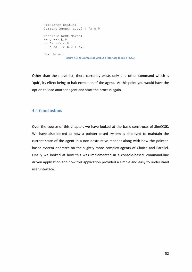
52
Simulator Status:
Current Agent: a.b.0 | ‘a.c.0
Possible Next Moves:
–- a --> b.0
–- ‘a --> c.0
-- t->a --> b.0 | c.0
Next Move:
Figure 4.3-2: Example of SimCCSK interface (a.b.0 + ‘a.c.0)
Other than the move list, there currently exists only one other command which is
‘quit’, its effect being to halt execution of the agent. At this point you would have the
option to load another agent and start the process again.
4.4 Conclusions
Over the course of this chapter, we have looked at the basic constructs of SimCCSK.
We have also looked at how a pointer-based system is deployed to maintain the
current state of the agent in a non-destructive manner along with how the pointer-
based system operates on the slightly more complex agents of Choice and Parallel.
Finally we looked at how this was implemented in a console-based, command-line
driven application and how this application provided a simple and easy to understand
user interface.
53
Chapter 5
WinSimCCSK
Over the course of this chapter we shall see how SimCCSK was adapted and extended
for a graphical world, resulting in WinSimCCSK. We then demonstrate WinSimCCSK’s
functionality by way of three examples.
5.1 SimCCSK for a More Colourful World
Had this project been undertaken 20 years ago, to a certain extent it would have been
console based as command line driven programs were fairly common place. However
fast forward 20 years and this is not the case, we now live in a more colourful world.
Graphical user interfaces are now common place with very few console based
applications. GUIs are on most users wish lists, since console based applications are
just a little alien now. This is of particular importance from a teaching standpoint as
the large majority of students grew up in a world populated with GUIs and that raises
the question of whether we are teaching them how to use a specific application or
whether we are trying to teach them a calculus. Clearly most students are likely to
feel more comfortable using a GUI based application. This is due to the reason that
GUI based applications will seem at least vaguely familiar and this of course would, to
a certain extent, get around the issue of trying to teach them the aspects and use of
the tool and allow the tool to aid them in their learning of process calculi. Based on
this idea WinSimCCSK was born.

54
WinSimCCSK is at its core the same application as SimCCSK, in fact the entire core
program is the same. The key difference is instead of a console based user interface
that sits on top of the core simulation system, this time around we have a GUI that sits
on top of it. The GUI links with the Simulator object in a similar way to its console
based counterpart. The GUI itself is built using .NET based around the design
proposed earlier, it features a collection of list boxes showing forward and reverse
moves and resulting agent expressions, in a similar way to the console based version.
It also includes the expression of the current agent again like in SimCCSK. In addition it
also includes a state history, showing in sequence every state visited thus providing
the route navigated through the agent. In order to assist with reference, the state
history also includes the key to the state on the graph (which will be discussed later in
this section). Finally, as has already been hinted at, there is the graph visualization and
key, linking the nodes on the graph to a state of the agent. It is also worth noting that
the window is resizable and that the components resize sensibly with it. For reference
we now include a screen shot of the main window on loading (with default agent 0).
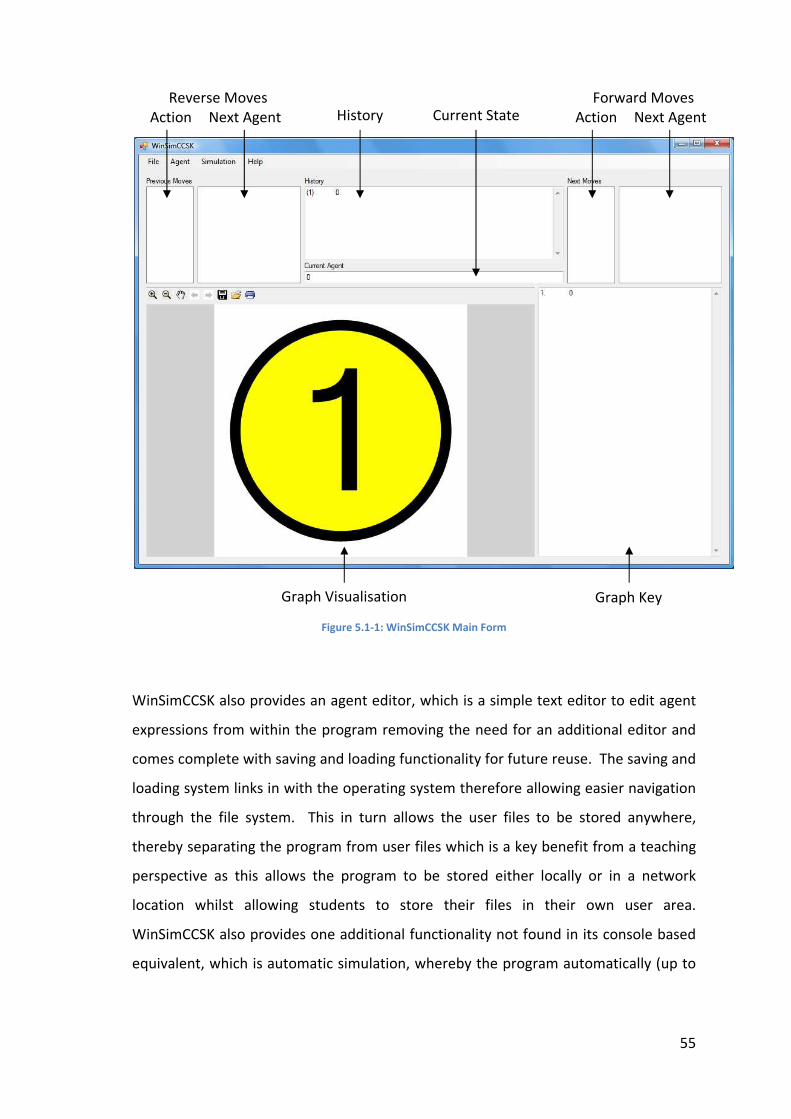
55
Figure 5.1-1: WinSimCCSK Main Form
WinSimCCSK also provides an agent editor, which is a simple text editor to edit agent
expressions from within the program removing the need for an additional editor and
comes complete with saving and loading functionality for future reuse. The saving and
loading system links in with the operating system therefore allowing easier navigation
through the file system. This in turn allows the user files to be stored anywhere,
thereby separating the program from user files which is a key benefit from a teaching
perspective as this allows the program to be stored either locally or in a network
location whilst allowing students to store their files in their own user area.
WinSimCCSK also provides one additional functionality not found in its console based
equivalent, which is automatic simulation, whereby the program automatically (up to
Graph Visualisation
Reverse Moves
Action Next Agent
Forward Moves
Action Next Agent History Current State
Graph Key

56
a certain depth), generates the graph of the agents’ possible movement, allowing a
quick way of seeing the behaviour of an agent.
The graph visualisation is a key component of WinSimCCSK and is generated using the
Microsoft Automatic Graph Layout (MSAGL) tool from Microsoft Research (Redmond).
It is currently being used in this project under an academic license. The MSAGL tool
provides two key advantages to the project. The first advantage is the integration of a
graph into the project. The graph component itself has two parts of interest. The first
is the graph itself which allows the construction of nodes and edges. The second is a
graph viewer, which comes with the added benefits of being able to save (and
subsequently load) the graph visualisation in two formats. The first format is to be
viewed from the graph viewer and as such within WinSimCCSK at a later date.
Although this graph would now be independent of the WinSimCCSK system, meaning
that you would only be able to view the graph as opposed to interactively navigate
through it. This would mean that the states of the system would not be reloaded in to
WinSimCCSK simulation engine. The alternative (and probably more useful in this
case) is the ability to export the graph as an image, thus allowing completed graphs to
be saved in a multi application and multi platform use.
The second advantage stems from the fact that given a graph MSAGL will always draw
the graph in a similar way, such that the overall structure of the graph will always look
the same although certain parts may be flipped around. This means that two or more
independent simulations of an agent, will result in a graph that structurally looks
identical with the exception that some of the parts and labels are moved around
(depending on execution order). This results in a positive benefit from a teaching tool
standpoint as this allows the students to easily reproduce the graphs regardless of the
execution order.
WinSimCCSK uses MSAGL to construct the graph using a combination of built in
methods and some additional custom ones, that aid in the navigation of previously
existing and visited nodes along with a couple that aid with the construction of edges
within previously existing nodes. Due to the nature of keys within CCSK, the only rule
being that they must be unique (or have only one matching in the case of
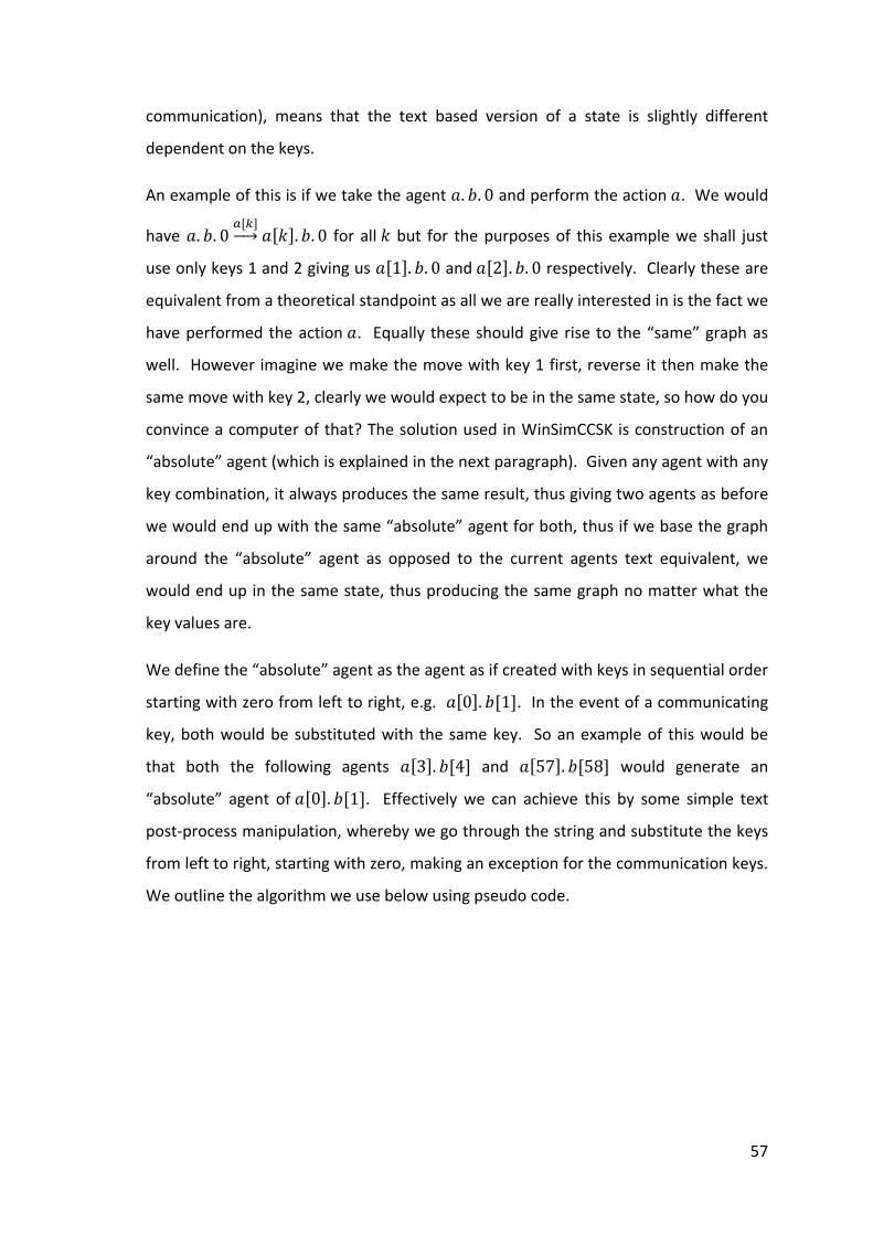
57
communication), means that the text based version of a state is slightly different
dependent on the keys.
An example of this is if we take the agent �. . 0 and perform the action �. We would
have �. . 0 0[T]>?@ �[S]. . 0 for all S but for the purposes of this example we shall just
use only keys 1 and 2 giving us �[1]. . 0 and �[2]. . 0 respectively. Clearly these are
equivalent from a theoretical standpoint as all we are really interested in is the fact we
have performed the action �. Equally these should give rise to the “same” graph as
well. However imagine we make the move with key 1 first, reverse it then make the
same move with key 2, clearly we would expect to be in the same state, so how do you
convince a computer of that? The solution used in WinSimCCSK is construction of an
“absolute” agent (which is explained in the next paragraph). Given any agent with any
key combination, it always produces the same result, thus giving two agents as before
we would end up with the same “absolute” agent for both, thus if we base the graph
around the “absolute” agent as opposed to the current agents text equivalent, we
would end up in the same state, thus producing the same graph no matter what the
key values are.
We define the “absolute” agent as the agent as if created with keys in sequential order
starting with zero from left to right, e.g. �[0]. [1]. In the event of a communicating
key, both would be substituted with the same key. So an example of this would be
that both the following agents �[3]. [4] and �[57]. [58] would generate an
“absolute” agent of �[0]. [1]. Effectively we can achieve this by some simple text
post-process manipulation, whereby we go through the string and substitute the keys
from left to right, starting with zero, making an exception for the communication keys.
We outline the algorithm we use below using pseudo code.
58
currentkey = 0;
foreach (token t in AgentString)
{
if(t is a Key)
{
if(t is in keylist)
{
AbsoluteString += keylist.newkey(t);
}
else
{
AbsoluteString += currentkey;
keylist.Add(t, currentkey);
currentkey++;
}
}
else
{
AbsoluteString += t;
}
}
Figure 5.1-2: Pseudo code for "absolute" Agent Generation
Now from a strict CCSK standpoint the first two agents are different and therefore
would produce different graphs, which would look identical just with different key
values. However for WinSimCCSK we take the idea of a visualisation as opposed to a
completely accurate graph. This is useful from a teaching standpoint as we are more
interested in the general layout of a graph for an agent than a specific graph and as
such are more interested in whether or not an action is keyed as opposed to the key
value. We can do this as the two graphs are similar. Using some thought out selection
of keys the same graph layout could be generated by hand. It is also worth noting that
we take this approach as currently WinSimCCSK allocates the keys automatically (again
sequentially from 0). Without this abstraction based on the concept of the fact that an
action is keyed as opposed to the value of the key being important, we avoid what
would be an infinitely branching graph. Every time we reversed a move we would be
unable to return to the previous state we were in as the key would be different, using
this abstract visually we return to the same state.
We then use the “absolute” agent as the value of any given node, thus creating a
visualisation based on the actions performed as opposed to the values of keys used.
However this clearly would make the graphs completely unreadable if we were to
label each node with the “absolute” agent. As such instead, as suggested earlier, we
59
use a key based system instead. Each time we visit a new node, we create a key for it
and add it to the key list, the keys are sequentially generated starting with one. After
every move, we generate the “absolute” agent and check for its presence in the key
list, if it already exists, we move to that node. If not we generate a new node and add
it to the graph.
5.2 Examples
Over the course of this section we shall look at several examples, illustrating
WinSimCCSK and some of its functionality.
5.2.1 The DNA System
Our first example is a simple one from molecular biology based around gene
expression (as taken and adapted from (7)). In this example, we have a complex
protein machinery (denoted by A) which has to bind to the DNA strand. However in
our example we have two inhibitors I1 and I2. I2 is trying to bind to the same site on
the DNA as A and I1, which if it binds to the DNA prevents the DNA from folding
correctly, which results in the gene not being expressed. The situation can be
summarized graphically as shown in Figure 5.2-1 (as taken and adapted from (7)).

60
Figure 5.2-1: Illustration of Gene Expression
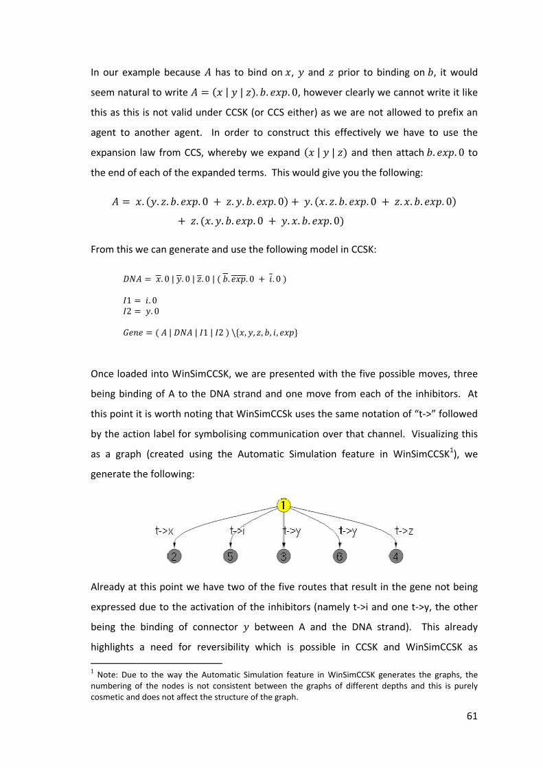
In our example because
seem natural to write
this as this is not v
agent to another a
expansion law from CCS, whereby we expand
the end of each of the expanded terms
� = .
From this we can generate and use
*]�
�1 =�2 =
^%"%
Once loaded into WinSimCCS
being binding of
this point it is worth noting that WinSimCCSk uses the same notation of
by the action label for symbolising communication over that channel
as a graph (created using the Automatic Simulation feature in WinSimCCSK
generate the following:
Already at this point we have two of the five routes that result in the gene not being
expressed due to the activation of the inhibitors (namely t
being the binding of connector
highlights a need for
1 Note: Due to the way the Automatic Simulation feature in WinSimCCSK generates the graphs, the
numbering of the nodes is not consistent
cosmetic and does not affect the structure of the graph.
In our example because � has to bind on
seem natural to write � = �. | B | _�. . %.#this as this is not valid under CCSK (or CCS either) as we are not allowed to prefix an
agent to another agent. In order to construct
expansion law from CCS, whereby we expand
the end of each of the expanded terms. This would give you the following:
.. �B. _. . %.#. 0 + _. B. . %.#+ _. �.. B. . %.#. 0 +
From this we can generate and use the following model in CCSK:
*]� = .. 0 | B. 0 | _. 0 | � . %.#. 0 + +.
= +. 0 = B. 0
^%"% = � � | *]� | �1 | �2 � \`., B, _, ,
Once loaded into WinSimCCSK, we are presented with the five possible moves, three
being binding of A to the DNA strand and one move from each of the inhibitors
this point it is worth noting that WinSimCCSk uses the same notation of
by the action label for symbolising communication over that channel
as a graph (created using the Automatic Simulation feature in WinSimCCSK
generate the following:
Already at this point we have two of the five routes that result in the gene not being
expressed due to the activation of the inhibitors (namely t
being the binding of connector B between A and the DNA
highlights a need for reversibility which is possible in CCSK and WinSimCCSK as
ue to the way the Automatic Simulation feature in WinSimCCSK generates the graphs, the
numbering of the nodes is not consistent between the graphs of different depths and this is purely
cosmetic and does not affect the structure of the graph.
to bind on ., B and _ prior to binding on
%.#. 0, however clearly we cannot write it like
alid under CCSK (or CCS either) as we are not allowed to prefix an
In order to construct this effectively we have to
expansion law from CCS, whereby we expand �. | B | _� and then attach
This would give you the following:
%.#. 0� + B. �.. _. . %.#. 0 + _. .+ B. .. . %.#. 0�
following model in CCSK:
. 0 �
+, %.#a
K, we are presented with the five possible moves, three
to the DNA strand and one move from each of the inhibitors
this point it is worth noting that WinSimCCSk uses the same notation of
by the action label for symbolising communication over that channel.
as a graph (created using the Automatic Simulation feature in WinSimCCSK
Already at this point we have two of the five routes that result in the gene not being
expressed due to the activation of the inhibitors (namely t->i and one t
between A and the DNA strand).
which is possible in CCSK and WinSimCCSK as
ue to the way the Automatic Simulation feature in WinSimCCSK generates the graphs, the
between the graphs of different depths and this is purely
cosmetic and does not affect the structure of the graph.
61
prior to binding on , it would
, however clearly we cannot write it like
alid under CCSK (or CCS either) as we are not allowed to prefix an
we have to use the
and then attach . %.#. 0 to
This would give you the following:
.. . %.#. 0�
K, we are presented with the five possible moves, three
to the DNA strand and one move from each of the inhibitors. At
this point it is worth noting that WinSimCCSk uses the same notation of “t->” followed
. Visualizing this
as a graph (created using the Automatic Simulation feature in WinSimCCSK1), we
Already at this point we have two of the five routes that result in the gene not being
>i and one t->y, the other
. This already
which is possible in CCSK and WinSimCCSK as
ue to the way the Automatic Simulation feature in WinSimCCSK generates the graphs, the
between the graphs of different depths and this is purely
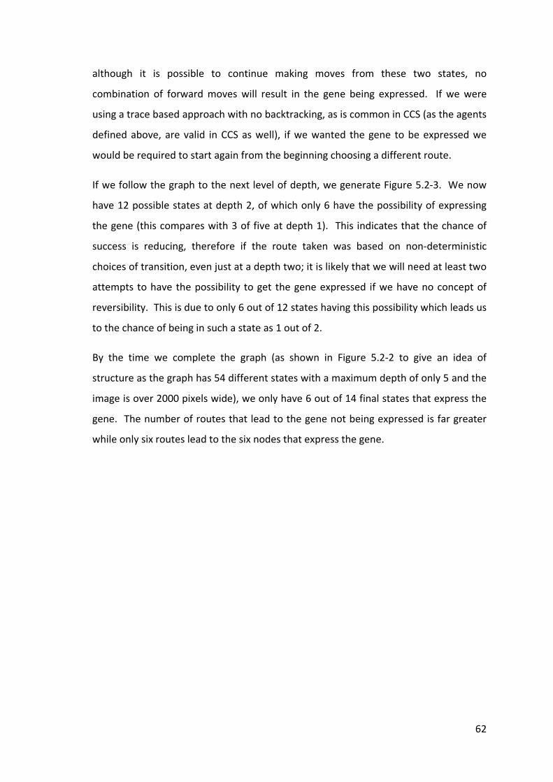
62
although it is possible to continue making moves from these two states, no
combination of forward moves will result in the gene being expressed. If we were
using a trace based approach with no backtracking, as is common in CCS (as the agents
defined above, are valid in CCS as well), if we wanted the gene to be expressed we
would be required to start again from the beginning choosing a different route.
If we follow the graph to the next level of depth, we generate Figure 5.2-3. We now
have 12 possible states at depth 2, of which only 6 have the possibility of expressing
the gene (this compares with 3 of five at depth 1). This indicates that the chance of
success is reducing, therefore if the route taken was based on non-deterministic
choices of transition, even just at a depth two; it is likely that we will need at least two
attempts to have the possibility to get the gene expressed if we have no concept of
reversibility. This is due to only 6 out of 12 states having this possibility which leads us
to the chance of being in such a state as 1 out of 2.
By the time we complete the graph (as shown in Figure 5.2-2 to give an idea of
structure as the graph has 54 different states with a maximum depth of only 5 and the
image is over 2000 pixels wide), we only have 6 out of 14 final states that express the
gene. The number of routes that lead to the gene not being expressed is far greater
while only six routes lead to the six nodes that express the gene.

Fig
ure
5.2
-3:
DN
A G
rap
h a
t d
ep
th o
f 2
63
Fig
ure
5.2
-2:
Co
mp
lete
DN
A G
rap
h

64
Now that we have seen the need for reversibility at a somewhat conceptual level, we
shall take a concrete example illustrating the advantage of reversibility as opposed to a
non-back tracking approach. Starting from the initial state we now present a possible
computation trace:
� � | *]� | �1 | �2 � \`., B, _, , +, %.#a 8[]>@
� .[1]. �B. _. . %.#. 0 + _. B. . %.#. 0� + B. �.. _. . %.#. 0 + _. .. . %.#. 0� + _. �.. B. . %.#. 0 + B. .. . %.#. 0�
| .[1].0 |B. 0 | _. 0 | b . %.#. 0 + +. 0 c
| �1 | �2 � \`., B, _, , +, %.#a 8[�]>@
� .[1]. �B[2]. _. . %.#. 0 + _. B. . %.#. 0� + B. �.. _. . %.#. 0 + _. .. . %.#. 0� + _. �.. B. . %.#. 0 + B. .. . %.#. 0�
| .[1].0 |B[2].0 | _. 0 | b . %.#. 0 + +. 0 c
| �1 | �2 � \`., B, _, , +, %.#a 8[N]>@
� .[1]. �B[2]. _[3]. . %.#. 0 + _. B. . %.#. 0� + B. �.. _. . %.#. 0 + _. .. . %.#. 0� + _. �.. B. . %.#. 0 + B. .. . %.#. 0�
| .[1].0 |B[2].0 | _[3].0 | b . %.#. 0 + +. 0 c
| �1 | �2 � \`., B, _, , +, %.#a 8[d]>@
� .[1]. �B[2]. _[3]. . %.#. 0 + _. B. . %.#. 0� + B. �.. _. . %.#. 0 + _. .. . %.#. 0� + _. �.. B. . %.#. 0 + B. .. . %.#. 0�
| .[1].0 |B[2].0 | _[3].0 | b . %.#. 0 + +[4].0 c
| +[4]. 0 | �2 � \`., B, _, , +, %.#a
At this point we are in the position whereby both the DNA and inhibitor I1 have
successfully bound to the DNA strand (as illustrated in Stage 1B in Figure 5.2-1). Due
to the inhibitor the DNA strand cannot fold properly to allow the binding of connector
and therefore the gene cannot be expressed.
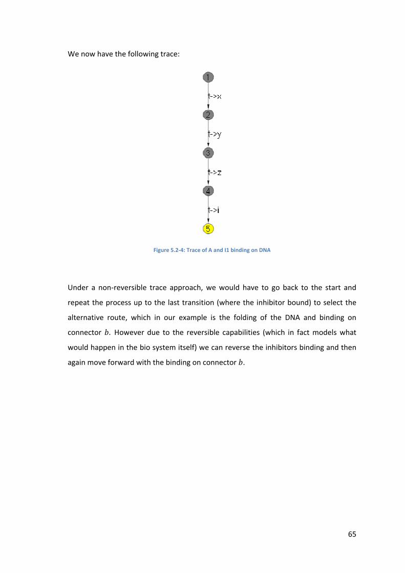
We now have the following trace:
Under a non
repeat the process up to the last transit
alternative route, whic
connector
would happen in the bio system itself)
again move forward with the
have the following trace:
Figure 5.2-4: Trace of A and I1 binding on DNA
Under a non-reversible trace approach, we would have to go back to the start and
repeat the process up to the last transit
alternative route, which in our example is the folding of the DNA and binding on
connector . However due to the reversible
would happen in the bio system itself) we
again move forward with the binding on connector
: Trace of A and I1 binding on DNA
trace approach, we would have to go back to the start and
repeat the process up to the last transition (where the inhibitor bound) to
h in our example is the folding of the DNA and binding on
reversible capabilities (which in fact model
we can reverse the inhibitors binding
binding on connector .
65
trace approach, we would have to go back to the start and
ion (where the inhibitor bound) to select the
h in our example is the folding of the DNA and binding on
(which in fact models what
can reverse the inhibitors binding and then

66
This leads to a successful expression of the gene, which can be observed in the
following computation:
[From Above]
⇝ 8[d]
� .[1]. �B[2]. _[3]. . %.#. 0 + _. B. . %.#. 0� + B. �.. _. . %.#. 0 + _. .. . %.#. 0� + _. �.. B. . %.#. 0 + B. .. . %.#. 0�
| .[1].0 |B[2].0 | _[3].0 | b . %.#. 0 + +. 0 c
| �1 | �2 � \`., B, _, , +, %.#a 8[e]>@
� .[1]. �B[2]. _[3]. [5]. %.#. 0 + _. B. . %.#. 0� + B. �.. _. . %.#. 0 + _. .. . %.#. 0�+ _. �.. B. . %.#. 0 + B. .. . %.#. 0�
| .[1].0 |B[2].0 | _[3].0 | b [5]. %.#. 0 + +. 0 c
| �1 | �2 � \`., B, _, , +, %.#a 8[f]>@
� .[1]. �B[2]. _[3]. [5]. exp[6].0 + _. B. . %.#. 0� + B. �.. _. . %.#. 0 + _. .. . %.#. 0�+ _. �.. B. . %.#. 0 + B. .. . %.#. 0�
| .[1].0 |B[2].0 | _[3].0 | b [5]. %.#[6].0 + +. 0 c
| �1 | �2 � \`., B, _, , +, %.#a
The above trace which contains reverse moves can be drawn as a graph (shown below
in Figure 5.2-5) with the successful expression of the gene. However it is worth noting
that the graph still shows that we visited the state in which the inhibitor had bound,
and indicates that we went back and took an alternative route.

Over the course of the relatively simple example we have seen how CCSK and in turn
WinSimCCSK can
as this biological system
backtracking in a process calculi helps better
5.2.2 The Jobshop
The second
which models a fairly simple production line; the pieces
called a job)
and then output
Jobbers) and two tools, a hammer and a mallet
by hand (for simple jobs), using a hammer (for hard jobs) or by using a tool
other jobs)
Figure 5.2-5: Trace back tracking binding of I1 to allow expression of gene
Over the course of the relatively simple example we have seen how CCSK and in turn
WinSimCCSK can allow for the easier modelling of system
as this biological system, it has also shown how the a
tracking in a process calculi helps better
The Jobshop
second example we shall look at is the Jobshop (as taken and adapted from
which models a fairly simple production line; the pieces
called a job) come in to the system, are constructed
and then output. The production line features two workers (which we shall call
Jobbers) and two tools, a hammer and a mallet
by hand (for simple jobs), using a hammer (for hard jobs) or by using a tool
other jobs). We shall assume that the distribution of easy, hard and all other jobs is
back tracking binding of I1 to allow expression of gene
Over the course of the relatively simple example we have seen how CCSK and in turn
allow for the easier modelling of systems prone to deadlocking such
, it has also shown how the additional functionality of
tracking in a process calculi helps better represent system’s behaviour.
example we shall look at is the Jobshop (as taken and adapted from
which models a fairly simple production line; the pieces (a base and a peg, together
come in to the system, are constructed into an object cal
The production line features two workers (which we shall call
Jobbers) and two tools, a hammer and a mallet. The construction is completed either
by hand (for simple jobs), using a hammer (for hard jobs) or by using a tool
We shall assume that the distribution of easy, hard and all other jobs is
67
back tracking binding of I1 to allow expression of gene
Over the course of the relatively simple example we have seen how CCSK and in turn
s prone to deadlocking such
dditional functionality of
represent system’s behaviour.
example we shall look at is the Jobshop (as taken and adapted from (1)),
(a base and a peg, together
object called done(job)
The production line features two workers (which we shall call
The construction is completed either
by hand (for simple jobs), using a hammer (for hard jobs) or by using a tool (for all
We shall assume that the distribution of easy, hard and all other jobs is
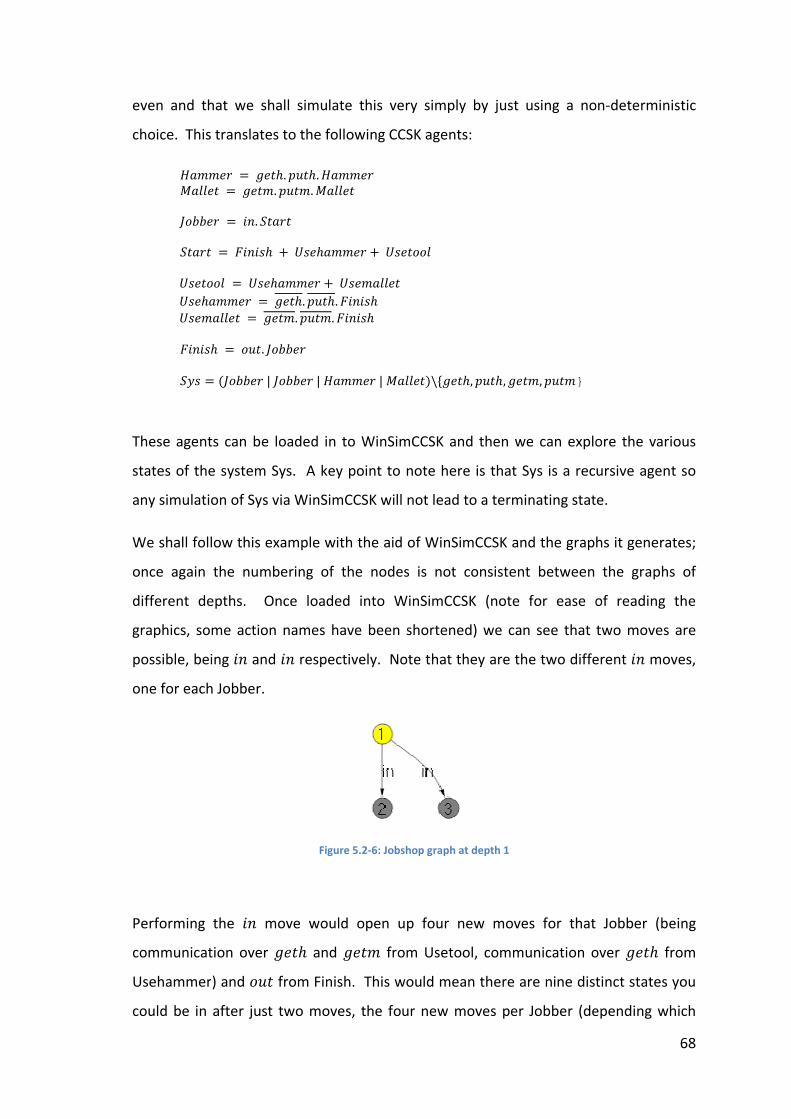
even and that we shall simulate this very simply by just using a non
choice. This translates to the following CCSK agents:
k�77%$ l�66%
m! %$
' �$
n&% !!6n&%n&%7�66%
o+"+&
'B&
These agents can be loaded in to
states of the system Sys
any simulation of Sys via WinSimCCSK will not lead to a terminating state
We shall follow this example with the aid o
once again
different depths
graphics, some action names have been shortened)
possible, being
one for each Jobber
Performing the
communication over
Usehammer
could be in after just tw
even and that we shall simulate this very simply by just using a non
This translates to the following CCSK agents:
k�77%$ = )% ℎ. #� ℎ. k�77%$
l�66% = )% 7. #� 7. l�66%
m! %$ = +". ' �$
' �$ = o+"+&ℎ + n&%ℎ�77%$ + n&% !!6
n&% !!6 = n&%ℎ�77%$ + n&%7�66% n&%ℎ�77%$ = )% ℎ. #� ℎ. o+"+&ℎ n&%7�66% = )% 7. #� 7. o+"+&ℎ
o+"+&ℎ = !� . m! %$
'B& = �m! %$ | m! %$ | k�77%$ | l�66%
These agents can be loaded in to WinSimCCSK and then we can explore
of the system Sys. A key point to note here is that
any simulation of Sys via WinSimCCSK will not lead to a terminating state
We shall follow this example with the aid o
again the numbering of the nodes is not consistent between the graphs of
different depths. Once loaded into WinSimCCSK
some action names have been shortened)
being +" and +" respectively. N
one for each Jobber.
Figure 5.2-6: Jobshop graph at depth 1
Performing the +" move would open up four
communication over )% ℎ and )% 7 from Usetool, communication over
Usehammer) and !� from Finish. This would mean there are nine distinct states you
could be in after just two moves, the four new moves per Jobber (depending which
even and that we shall simulate this very simply by just using a non
This translates to the following CCSK agents:
n&% !!6
n&%7�66%
l�66% �\`)% ℎ, #� ℎ, )% 7, #� 7}
WinSimCCSK and then we can explore
A key point to note here is that Sys is a recursive agent so
any simulation of Sys via WinSimCCSK will not lead to a terminating state
We shall follow this example with the aid of WinSimCCSK and the graphs it generates
the numbering of the nodes is not consistent between the graphs of
Once loaded into WinSimCCSK (note for ease of reading the
some action names have been shortened) we can see that two moves are
Note that they are the two different
: Jobshop graph at depth 1
open up four new moves for that
from Usetool, communication over
This would mean there are nine distinct states you
o moves, the four new moves per Jobber (depending which
68
even and that we shall simulate this very simply by just using a non-deterministic
WinSimCCSK and then we can explore the various
Sys is a recursive agent so
any simulation of Sys via WinSimCCSK will not lead to a terminating state.
f WinSimCCSK and the graphs it generates;
the numbering of the nodes is not consistent between the graphs of
(note for ease of reading the
that two moves are
ote that they are the two different +" moves,
Jobber (being
from Usetool, communication over )% ℎ from
This would mean there are nine distinct states you
o moves, the four new moves per Jobber (depending which

made the first move
Jobbers just making their first move only.
From here each state which saw a single Jobber make two moves then h
coming from it;
or getting a new job in, along with the other Jobber getting a new j
sixteen new states
Jobbers have
four for Jobber two)
sixteen as
and either picked up a tool or finished it, and the other Jobber having just picked up a
job.
made the first move as described above
Jobbers just making their first move only.
Figure 5.2-7: Jobshop
From here each state which saw a single Jobber make two moves then h
coming from it; one being the next move of that Jobber, either putting the tool down
or getting a new job in, along with the other Jobber getting a new j
sixteen new states. The remaining state
have taken a job in, leads to one of eight states (four being for Jo
four for Jobber two). Of course these eight states overlap the
sixteen as these would cover the same positions as one Jobber having picked up a job
and either picked up a tool or finished it, and the other Jobber having just picked up a
as described above) along with the remaining possibility of both
Jobbers just making their first move only.
: Jobshop graph at depth 2
From here each state which saw a single Jobber make two moves then h
next move of that Jobber, either putting the tool down
or getting a new job in, along with the other Jobber getting a new job in, giving us
The remaining state (from the previous group) being where both
leads to one of eight states (four being for Jo
course these eight states overlap the previously stated
these would cover the same positions as one Jobber having picked up a job
and either picked up a tool or finished it, and the other Jobber having just picked up a
69
) along with the remaining possibility of both
From here each state which saw a single Jobber make two moves then has possibilities
next move of that Jobber, either putting the tool down
ob in, giving us
being where both
leads to one of eight states (four being for Jobber one,
previously stated
these would cover the same positions as one Jobber having picked up a job
and either picked up a tool or finished it, and the other Jobber having just picked up a

Fig
ure
5.2
-8:
Job
sho
p G
rap
h a
t d
ep
th 3
70

71
Already at this point the graph (Figure 5.2-8) is becoming quite large (the above
images are scaled to fit the page up to actual size), the above image for example has
been shrunk to just 45% of its original size, the bitmap version of the above graph
measures over 2000 pixels wide.
Over the course of depths four and five we add 33 and 60 new nodes respectively,
meaning at depth five we now have 121 nodes and a graph 8,500 pixels wide which is
over four times the pixel width of depth three.
At this point we can start to see a pattern emerging in the progression of this agent,
for each level of depth the new number of nodes added are roughly double the
number the previous depth added. This results in our graph’s width matching this
growth again roughly doubling at each level of depth. By depths nine and ten we have
reached a total of 1425 and 2536 nodes in total respectively with graph widths of
140,000 and 260,000 pixels respectively, these show that the system is able to cope
with agents and graphs of reasonable size and complexity.
Using the Jobshop as our test agent, we collected data based on the automatic
simulation of the agent to varying depths (ranging from 0 – 10) in order to test the
system’s functionality at handling ever larger agent information and ever growing
graphs. As part of the test we measured the number of nodes created in the graph
(which in turn gives us the number of new nodes) and the time taken to perform the
automatic simulation on our test PC. The time taken is calculated using an internal
timer within the program as it is part of the automatic simulation functionality. The
test PC uses an Intel Core2 Quad processor running at 2.4GHz with 2GB of RAM
running Windows Vista (32-bit) and .NET 3.5. A key point is that despite running the
tests on a quad core machine, it is worth noting that WinSimCCSK is currently a non-
threaded application and therefore only utilizes one of the four cores during testing.
Hence the only benefit from running the tests on a multi core machine is that system
tasks can be executed on a different core, which should give WinSimCCSK near enough
uninterrupted use of one core.

72
Depth Total New Time
0 1 1 00:00:00
1 3 2 00:00:01
2 12 9 00:00:06
3 28 16 00:00:23
4 61 33 00:01:06
5 121 60 00:03:07
6 240 119 00:11:14
7 438 198 00:30:41
8 793 355 01:45:19
9 1425 632 06:04:52
10 2536 1111 22:33:22
Nodes
Figure 5.2-9: Data Collected from Jobshop
As suggested previously we can see that the number of nodes roughly doubles at each
depth. The time on the other hand expands using a much larger factor being roughly
3.5. This means that while WinSimCCSK is able to handle the larger graphs it is often
going to be time that is the major constraint on it. At depths nine and ten, we are
looking at 6 and 22 hours respectively, which are both relatively long times, however
one would have to compare that to the time it would take to draw such graphs by
hand. WinSimCCSK is clearly going to be both much quicker and more accurate due to
the sheer scale of it, at a depth of 8, the graph has nearly 800 states and took under
two hours to generate. It is worth noting that the depth of 8 is an important one, as
only after eight moves are we guaranteed to have a particular job completed. This is
of course based on both jobbers using a tool (which is four moves) and the second
jobber completing their job before the first jobber, hence eight. This shows one of the
major advantages of using a tool such as WinSimCCSK. However clearly the current
prototype still has a few shortcomings in performance. In this example it is fairly clear
that the depth of ten would really be a limit in practical terms, as nearly taking a day to
generate a graph is a long time.
Of course it is fairly obvious that the Jobshop example does not require any
reversibility, as in the event the tool required is in use, the other jobber clearly just
needs to wait for the first to finish before carrying on. However, that does not mean

73
that the Jobshop is a poor example to use. Previously we have mentioned how
WinSimCCSK could be used to aid the teaching of process calculi to students, this is
one such example. The Jobshop is a fairly classic example from the world of CCS and
as such it would not be out of place in a course teaching CCS to students. The added
benefit of reversibility allows the students to effectively undo their choices and allow
them to see the effect of a different choice, whilst still being able to see their previous
choices (including the undone ones) in the graph. It is also worth noting that both
Concurrency Workbench and FDR2 do not have anything similar to this visual
exploration (that maintains previous choices) as well as any form of automatic
generation of such a visualisation.
5.2.3 The Dining Philosophers
The third example we shall look at is the classic example of the dining philosophers
(36). For completeness, we will briefly outline the problem here. Five philosophers sit
around a table and do one of two things, thinking or eating. They do not do both at
the same time and as such do either one or the other. In the middle of the table is a
bowl of rice, on each side of each philosopher is a chopstick, which they share with
their neighbour. In order to eat they need to pick up both chopsticks. They also do
not talk to one another and therefore cannot ask their neighbour about the chopstick.
We will simplify this problem slightly by dictating that each philosopher must pick up
their right chopstick first. We can model this in CCSK using the following agents:
' +�S1 = �1. �1. ' +�S1 ' +�S2 = �2. �2. ' +�S2 ' +�S3 = �3. �3. ' +�S3 ' +�S4 = �4. �4. ' +�S4 ' +�S5 = �5. �5. ' +�S5
p� 6% = ' +�S1 | ' +�S2 | ' +�S3 | ' +�S4 | ' +�S5
�� 1 = ′�1. ′�2. %� 1. ′�1. ′�2. �ℎ+61 �� 2 = ′�2. ′�3. %� 2. ′�2. ′�3. �ℎ+62 �� 3 = ′�3. ′�4. %� 3. ′�3. ′�4. �ℎ+63 �� 4 = ′�4. ′�5. %� 4. ′�5. ′�5. �ℎ+64 �� 5 = ′�5. ′�1. %� 5. ′�5. ′�1. �ℎ+65

74
pℎ+"S1 = ℎ+"S1. �ℎ+61 pℎ+"S2 = ℎ+"S2. �ℎ+62 pℎ+"S3 = ℎ+"S3. �ℎ+63 pℎ+"S4 = ℎ+"S4. �ℎ+64 pℎ+"S5 = ℎ+"S5. �ℎ+65
�ℎ+61 = pℎ+"S1 + �� 1 �ℎ+62 = pℎ+"S2 + �� 2 �ℎ+63 = pℎ+"S3 + �� 3 �ℎ+64 = pℎ+"S4 + �� 4 �ℎ+65 = pℎ+"S5 + �� 5
�!!7 = � �ℎ+61 | �ℎ+62 | �ℎ+63 | �ℎ+64 | �ℎ+65 | p� 6% �
\`�1, �2, �3, �4, �5, �1, �2, �3, �4, �5a
We have specified the number of the chopstick being equal to the number of the
philosopher to which it is directly to the right of. We have also shortened the names
of the actions for picking up and putting down the chopstick to u and d respectively.
The philosophers are numbered in a clockwise fashion.
For the most part the Room agent runs well and reversibility is not needed. However
there is one particular case when reversibility is needed to overcome a deadlock
situation. This situation is when all five philosophers decided to eat at the same time
and as such they will all pick up their right chopstick. However because they have all
picked up their right chopsticks, all chopsticks are now in use. This means that none of
the philosophers can pick up their left chopstick and eat. We are now in situation
similar to the following:
� ℎ+"S1. �ℎ+61 + ′�1[0]. ′�2. %� 1. ′�1. ′�2. �ℎ+61� | � ℎ+"S2. �ℎ+62 + ′�2[1]. ′�3. %� 2. ′�2. ′�3. �ℎ+62� | � ℎ+"S3. �ℎ+63 + ′�3[2]. ′�4. %� 3. ′�3. ′�4. �ℎ+63� | � ℎ+"S4. �ℎ+64 + ′�4[3]. ′�5. %� 4. ′�5. ′�5. �ℎ+64� | � ℎ+"S5. �ℎ+65 + ′�5[4]. ′�1. %� 5. ′�5. ′�1. �ℎ+65� | ��1[0]. �1. ' +�S1 | �2[1]. �2. ' +�S2 | �3[2]. �3. ' +�S3 | �4[3]. �4. ' +�S4 | �5[4]. �5. ' +�S5�
\`�1, �2, �3, �4, �5, �1, �2, �3, �4, �5a
To solve this problem, one philosopher needs to put down their chopstick. In a
forward move only world this is not possible as they can only put down their
chopsticks after eating, which is currently not possible. What really needs to happen is
for one philosopher to undo the decision they made to pick up the chopstick and put it
down. This of course requires a reverse move. If we assume philosopher one makes
this move, from our previous state we arrive here:

75
� ℎ+"S1. �ℎ+61 + ′�1. ′�2. %� 1. ′�1. ′�2. �ℎ+61� | � ℎ+"S2. �ℎ+62 + ′�2[1]. ′�3. %� 2. ′�2. ′�3. �ℎ+62� | � ℎ+"S3. �ℎ+63 + ′�3[2]. ′�4. %� 3. ′�3. ′�4. �ℎ+63� | � ℎ+"S4. �ℎ+64 + ′�4[3]. ′�5. %� 4. ′�5. ′�5. �ℎ+64� | � ℎ+"S5. �ℎ+65 + ′�5[4]. ′�1. %� 5. ′�5. ′�1. �ℎ+65� | ��1. �1. ' +�S1 | �2[1]. �2. ' +�S2 | �3[2]. �3. ' +�S3 | �4[3]. �4. ' +�S4 | �5[4]. �5. ' +�S5�
\`�1, �2, �3, �4, �5, �1, �2, �3, �4, �5a
From this point we can see that chopstick one is now free again and so philosopher
five (the one being to philosopher one’s right) can now continue. When finished,
philosopher four can continue and so on until philosopher two finishes and all
chopsticks are down. At this point both chopsticks would be available to philosopher
one and the deadlock has been resolved. Of course under this scenario we could have
quite easily reversed any of the philosophers not just number one, equally we could
have reversed more than one too, although after the first, the deadlock would have
already been lifted. Graphically this entire process would have generated this graph
(Figure 5.2-10).
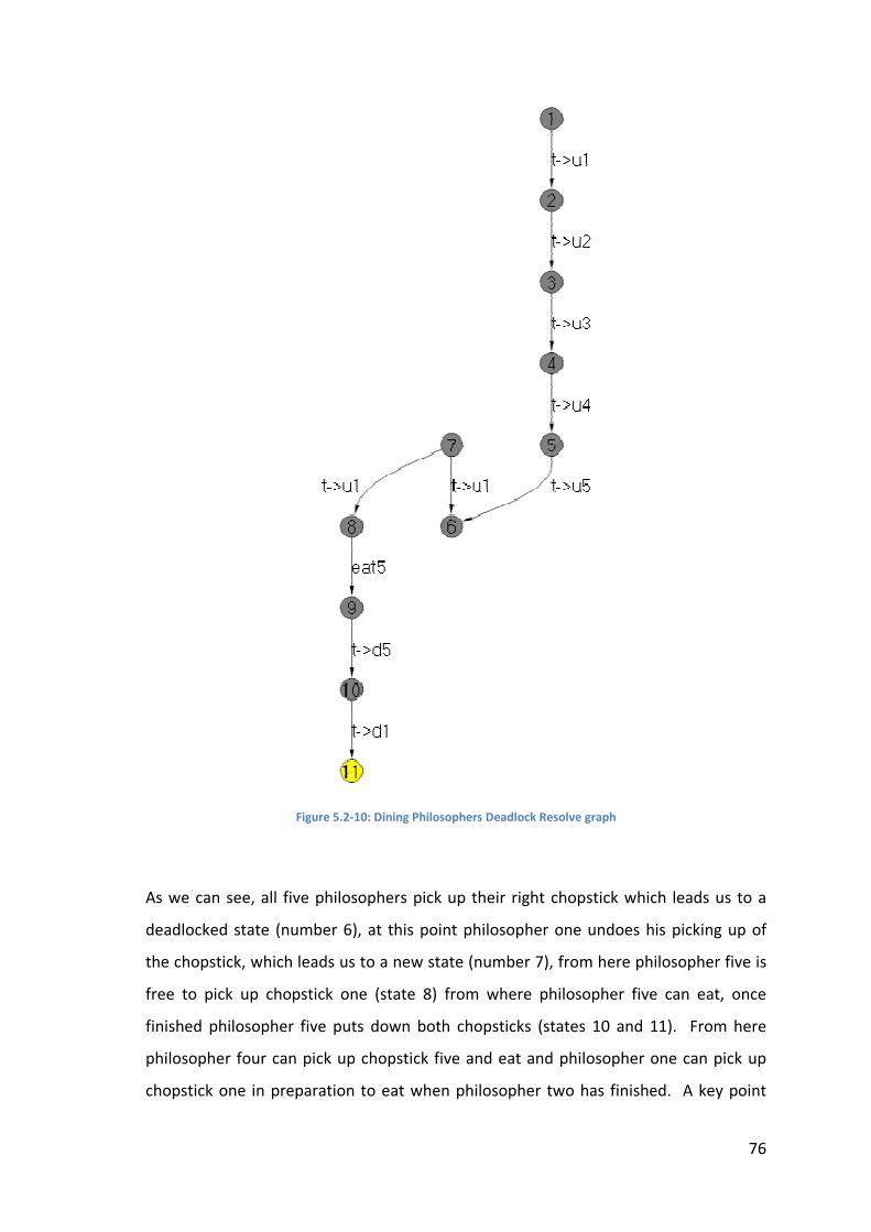
As we can see
deadlocked state (number 6), at this point philosopher one undoes his picking up of
the chopstick, which leads us to a new state (number 7), from here philosopher five is
free to pick up chopstick one (state 8) from where philosopher five can eat, o
finished philosopher five puts down both chopsticks (states 10 and 11)
philosopher four can pick
chopstick
Figure 5.2-10: Dining Philosophers Deadlock Resolve graph
As we can see, all five philosophers pick up their right chopstick which leads u
deadlocked state (number 6), at this point philosopher one undoes his picking up of
the chopstick, which leads us to a new state (number 7), from here philosopher five is
free to pick up chopstick one (state 8) from where philosopher five can eat, o
finished philosopher five puts down both chopsticks (states 10 and 11)
philosopher four can pick up chopstick five and eat and philosopher one can pick up
one in preparation to eat when philosopher two has finished
: Dining Philosophers Deadlock Resolve graph
pick up their right chopstick which leads u
deadlocked state (number 6), at this point philosopher one undoes his picking up of
the chopstick, which leads us to a new state (number 7), from here philosopher five is
free to pick up chopstick one (state 8) from where philosopher five can eat, o
finished philosopher five puts down both chopsticks (states 10 and 11)
chopstick five and eat and philosopher one can pick up
in preparation to eat when philosopher two has finished
76
pick up their right chopstick which leads us to a
deadlocked state (number 6), at this point philosopher one undoes his picking up of
the chopstick, which leads us to a new state (number 7), from here philosopher five is
free to pick up chopstick one (state 8) from where philosopher five can eat, once
finished philosopher five puts down both chopsticks (states 10 and 11). From here
chopstick five and eat and philosopher one can pick up
in preparation to eat when philosopher two has finished. A key point
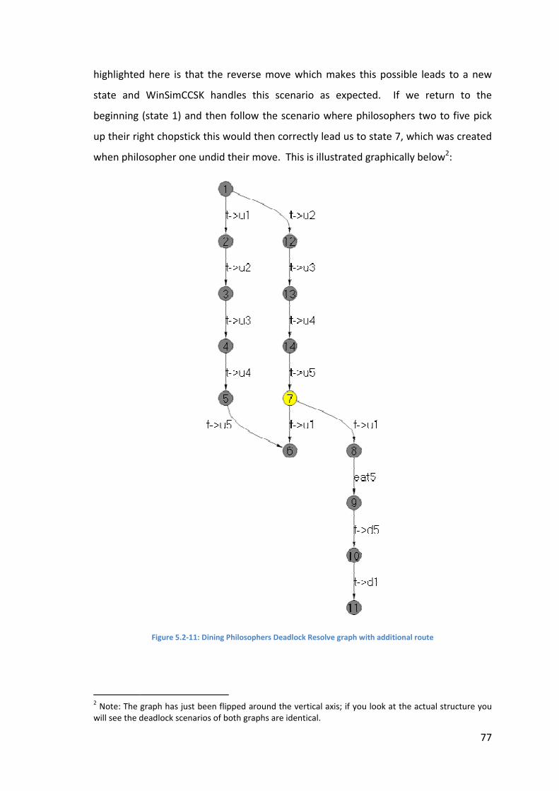
highlighted here is that the reverse move which make
state and
beginning (state 1) and then follow
up their rig
when philosopher one undid their move
2 Note: The graph has just been flipped around the vertical axis; if you look at the actual structure you
will see the deadlock scenarios of
ighlighted here is that the reverse move which make
WinSimCCSK handles this scenario as expected
ning (state 1) and then follow the scenario where philosophers two to five pick
up their right chopstick this would then correctly lead us to state 7, which was created
when philosopher one undid their move.
Figure 5.2-11: Dining Philosophers Deadlock
Note: The graph has just been flipped around the vertical axis; if you look at the actual structure you
will see the deadlock scenarios of both graphs are identical.
ighlighted here is that the reverse move which makes this possible leads to a new
WinSimCCSK handles this scenario as expected. If we return to the
the scenario where philosophers two to five pick
ht chopstick this would then correctly lead us to state 7, which was created
. This is illustrated graphically below
Dining Philosophers Deadlock Resolve graph with additional route
Note: The graph has just been flipped around the vertical axis; if you look at the actual structure you
both graphs are identical.
77
s possible leads to a new
If we return to the
the scenario where philosophers two to five pick
ht chopstick this would then correctly lead us to state 7, which was created
This is illustrated graphically below2:
with additional route
Note: The graph has just been flipped around the vertical axis; if you look at the actual structure you
78
Over the course of this classic example, we have again seen the benefit of reversibility
along with WinSimCCSK’s handling of scenarios when a reverse move may not
necessarily be the last. This is often the case when dealing with multiple agents in
parallel and using some form of a shared resource. We have then seen how this state
can then be linked up via another route if the sequence of events was different and
yet led to the same scenario, in our case philosophers two to five have one chopstick
each.
5.3 Conclusions
In this chapter we have looked at the alterations and extensions for putting SimCCSK
into a graphical world, resulting in WinSimCCSK. We looked at how a graph was
included and how the required us to generate an “absolute” agent, which we
explained the process of genrating. We went on to look at three examples which we
used to illustrate the functionality of WinSimCCSK, in particular the graph generation
and highlighting its handling of certain scenarios.

79
Chapter 6
User Guide
Over this relatively short chapter, we present a simple user guide for WinSimCCSK,
explaining its usage and finishing with a simple step by step tutorial example.
6.1 Requirements
The system requirements for SimCCSK and WinSimCCSK are as follows:
• .NET Framework 2.0 runtime
• Windows 98 (or higher)
6.2 Setting up WinSimCCSK
WinSimCCSK comes packaged in a self-extracting installer. To install the package, run
‘setup.exe’ and follow the onscreen instructions. Once installed you can start
WinSimCCSK by either running WinSimCCSK from the Start menu or alternatively by
running the WinSimCCSK.exe file from the WinSimCCSK folder within your file system.
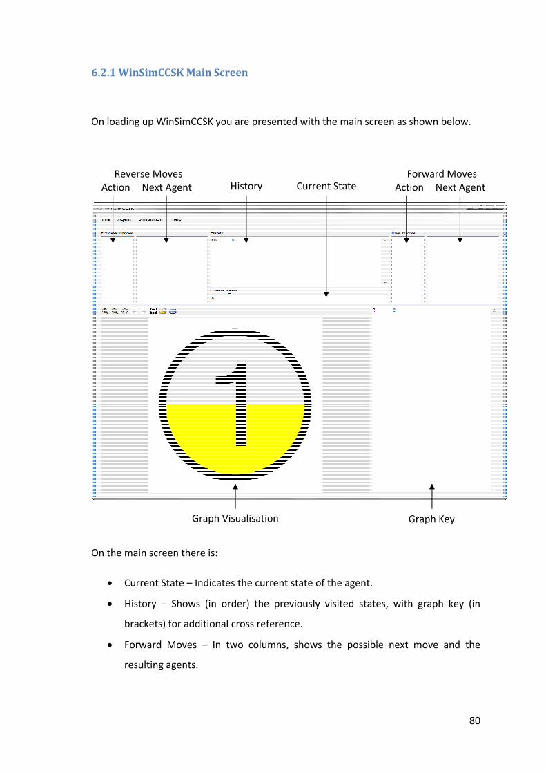
6.2.1 WinSimCCSK Main Screen
On loading up WinSimCCSK you are presented with the main screen as
On the main screen there is:
• Current State
• History
brackets)
• Forward Moves
resulting agent
Reverse Moves
Action
WinSimCCSK Main Screen
On loading up WinSimCCSK you are presented with the main screen as
On the main screen there is:
Current State – Indicates the current state of
History – Shows (in order) the previously visited states
brackets) for additional cross reference
Forward Moves – In two columns, shows the possible n
resulting agents.
Graph Visualisation
Reverse Moves
Next Agent History
On loading up WinSimCCSK you are presented with the main screen as shown below.
Indicates the current state of the agent.
Shows (in order) the previously visited states, with graph key
for additional cross reference.
In two columns, shows the possible next move
Graph Visualisation
Forward Moves
ActionCurrent State
Graph Key
80
shown below.
, with graph key (in
ext move and the
Forward Moves
Action Next Agent
Graph Key
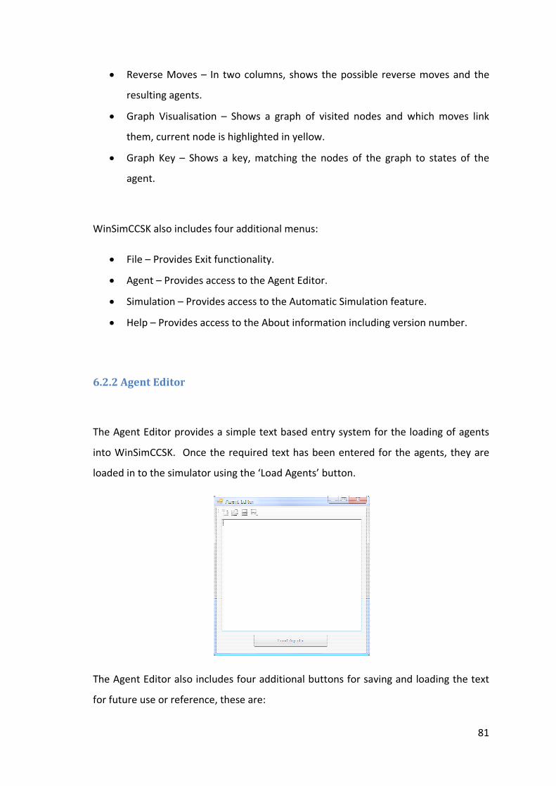
• Reverse Moves
resulting agent
• Graph Visualisation
them, current
• Graph Key
agent.
WinSimCCSK also includes four additional menus:
• File
• Agent
• Simulation
• Help
6.2.2 Agent Editor
The Agent Editor provides a simple text based entry system for
into WinSimCCSK
loaded in to the simulator using the ‘Load Agents’ button
The Agent Editor also includes four additional buttons for saving and loading the text
for future use or reference, these are:
Reverse Moves – In two columns, shows t
resulting agents.
Graph Visualisation – Shows a graph of visited nodes and which moves link
them, current node is highlighted in yellow.
Graph Key – Shows a key, matching the nodes of the graph to states of the
agent.
SimCCSK also includes four additional menus:
File – Provides Exit functionality.
Agent – Provides access to the Agent Editor.
Simulation – Provides access to the Automatic Simulation feature.
Help – Provides access to the About
Agent Editor
The Agent Editor provides a simple text based entry system for
into WinSimCCSK. Once the required text has been entered for the agents, they are
loaded in to the simulator using the ‘Load Agents’ button
The Agent Editor also includes four additional buttons for saving and loading the text
for future use or reference, these are:
In two columns, shows the possible reverse moves and
Shows a graph of visited nodes and which moves link
node is highlighted in yellow.
Shows a key, matching the nodes of the graph to states of the
SimCCSK also includes four additional menus:
Provides access to the Agent Editor.
Provides access to the Automatic Simulation feature.
Provides access to the About information including versio
The Agent Editor provides a simple text based entry system for the loading of agents
Once the required text has been entered for the agents, they are
loaded in to the simulator using the ‘Load Agents’ button.
The Agent Editor also includes four additional buttons for saving and loading the text
81
he possible reverse moves and the
Shows a graph of visited nodes and which moves link
Shows a key, matching the nodes of the graph to states of the
Provides access to the Automatic Simulation feature.
including version number.
loading of agents
Once the required text has been entered for the agents, they are
The Agent Editor also includes four additional buttons for saving and loading the text

82
• New – This will create a new file.
• Open – Load an existing file.
• Save – Saves the text to the current file and will overwrite the file if it already
exists. Will prompt for name if no current file is specified.
• SaveAs – Saves the text to a specified file and will overwrite the file if it already
exists.
Agents are typed using CCSK syntax, just as one would on paper. We shall quickly go
over the various components and how they can be entered in to WinSimCCSK.
Actions – Actions are specified using a text label, however, the following conditions
must be observed. Actions must start with a lower case letter and cannot include
spaces or any other reserved character, e.g. “a” . Overbar actions can be specified by
prefixing a single quote “ ‘ “ in front of the label, e.g. “ ‘a”.
Zero Agent – The Zero agent is specified using the Zero character ‘0’.
Prefixing – Prefixing is specified using a period ‘.’, e.g. “a.b.0”
Choice – Choice is specified using the plus symbol ‘+’, e.g. “a.b.0 + c.d.0”
Parallel – Parallel is specified using a vertical bar ‘|’, e.g. “a.b.0 | c.d.0”
Brackets – Brackets can be used to change the order of binding of operators, specified
using ‘(‘ and ‘)’, e.g. “(a.b.0)”
Restriction – Restriction is used to restrict actions from being executed independently,
thus allowing for communication only. It is specified using a backslash ‘\’ followed by
either a single action or by multiple actions which can be specified using curly brackets
‘{‘ and ‘}’ surrounding a list of actions by commas ‘,’. Examples “(a.b.0)\b” or
“(a.b.0)\{b,c}”
Relabelling – Relabeling allows one or more actions to be symbolically relabelled to
other actions. This is specified using square brackets ‘[‘ and ‘]’ which contain the new
label followed by a forward slash ‘/’ then the existing label. Multiple re-labels can be
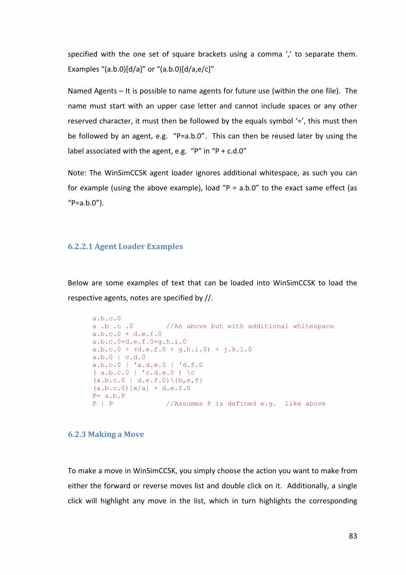
83
specified with the one set of square brackets using a comma ‘,’ to separate them.
Examples “(a.b.0)[d/a]” or “(a.b.0)[d/a,e/c]”
Named Agents – It is possible to name agents for future use (within the one file). The
name must start with an upper case letter and cannot include spaces or any other
reserved character, it must then be followed by the equals symbol ‘=’, this must then
be followed by an agent, e.g. “P=a.b.0”. This can then be reused later by using the
label associated with the agent, e.g. “P” in “P + c.d.0”
Note: The WinSimCCSK agent loader ignores additional whitespace, as such you can
for example (using the above example), load “P = a.b.0” to the exact same effect (as
“P=a.b.0”).
6.2.2.1 Agent Loader Examples
Below are some examples of text that can be loaded into WinSimCCSK to load the
respective agents, notes are specified by //.
a.b.c.0
a .b .c .0 //As above but with additional whitespace
a.b.c.0 + d.e.f.0
a.b.c.0+d.e.f.0+g.h.i.0
a.b.c.0 + (d.e.f.0 + g.h.i.0) + j.k.l.0
a.b.0 | c.d.0
a.b.c.0 | 'a.d.e.0 | 'd.f.0
( a.b.c.0 | 'c.d.e.0 ) \c
(a.b.c.0 | d.e.f.0)\{b,e,f}
(a.b.c.0)[x/a] + d.e.f.0
P= a.b.P
P | P //Assumes P is defined e.g. like above
6.2.3 Making a Move
To make a move in WinSimCCSK, you simply choose the action you want to make from
either the forward or reverse moves list and double click on it. Additionally, a single
click will highlight any move in the list, which in turn highlights the corresponding

resulting agent
agent.
After selecting a move, the screen is updated with the new state of the agent, the
possible move lists are updated too and the graph is updated eithe
or edge, or simply the currently selected
6.3 Automatic S
From within the ‘Simulation’ menu, there is the option of ‘Automatic Simulation’
This option allows the automatic simulation of an agent in order to generate a
complete graph of
being the
the depth)
value of 10
used, the automatic simulation can take a long time (up to several hours or even
longer) and
has crashed
After generation you will be in the
(even adding additional nodes if you progress past the depth used in the automatic
simulation) and have access to the rest of the functionality in WinSimCCSK including
the ability to save the graph.
resulting agent. Conversely, it is possible to select the move by selecting the
After selecting a move, the screen is updated with the new state of the agent, the
possible move lists are updated too and the graph is updated eithe
or edge, or simply the currently selected
Automatic Simulation
From within the ‘Simulation’ menu, there is the option of ‘Automatic Simulation’
This option allows the automatic simulation of an agent in order to generate a
complete graph of the movements within the agent up to
the number of forward moves made from the start
). This depth is specified by the
value of 10. Please note that depending on the
used, the automatic simulation can take a long time (up to several hours or even
longer) and due to the non-responsiveness
has crashed.
After generation you will be in the initial
(even adding additional nodes if you progress past the depth used in the automatic
simulation) and have access to the rest of the functionality in WinSimCCSK including
the ability to save the graph.
it is possible to select the move by selecting the
After selecting a move, the screen is updated with the new state of the agent, the
possible move lists are updated too and the graph is updated either with a new node
or edge, or simply the currently selected node is changed.
From within the ‘Simulation’ menu, there is the option of ‘Automatic Simulation’
This option allows the automatic simulation of an agent in order to generate a
the movements within the agent up to a specified depth (the depth
made from the start and reverse moves reduce
This depth is specified by the user; however there is also a preset default
Please note that depending on the complexity of the agent and the depth
used, the automatic simulation can take a long time (up to several hours or even
responsiveness can give the impression that WinSimCCSK
initial state and can move through the agent freely
(even adding additional nodes if you progress past the depth used in the automatic
simulation) and have access to the rest of the functionality in WinSimCCSK including
84
it is possible to select the move by selecting the resulting
After selecting a move, the screen is updated with the new state of the agent, the
r with a new node
From within the ‘Simulation’ menu, there is the option of ‘Automatic Simulation’.
This option allows the automatic simulation of an agent in order to generate a
specified depth (the depth
reverse moves reduce
however there is also a preset default
the agent and the depth
used, the automatic simulation can take a long time (up to several hours or even
give the impression that WinSimCCSK
can move through the agent freely
(even adding additional nodes if you progress past the depth used in the automatic
simulation) and have access to the rest of the functionality in WinSimCCSK including
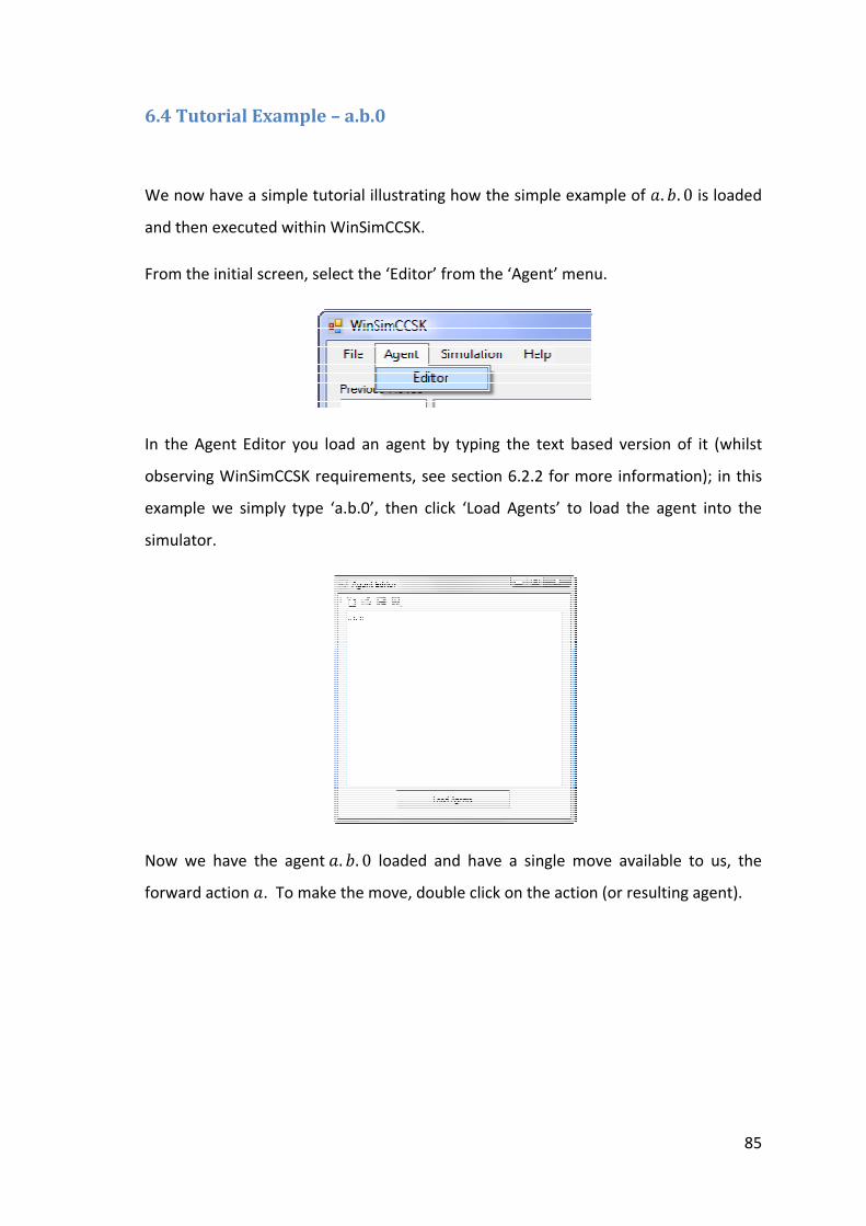
6.4 Tutorial Example
We now have a simple tutorial illustrating how the simple example of
and then executed within WinSimCCSK.
From the initial screen, select the ‘Editor’ from the ‘Agent’ menu.
In the Agent Editor you load an agent by typing the text based version of it (whilst
observing WinSimCCSK requirements, see section
example we simply type ‘a.b.0’, the
simulator.
Now we have the agent
forward action
Tutorial Example – a.b.0
We now have a simple tutorial illustrating how the simple example of
and then executed within WinSimCCSK.
From the initial screen, select the ‘Editor’ from the ‘Agent’ menu.
In the Agent Editor you load an agent by typing the text based version of it (whilst
observing WinSimCCSK requirements, see section
example we simply type ‘a.b.0’, then click ‘Load Agents’ to load the agent into the
Now we have the agent �. . 0 loaded and have a single move available to us, the
action �. To make the move, double click on the action (or
We now have a simple tutorial illustrating how the simple example of �
From the initial screen, select the ‘Editor’ from the ‘Agent’ menu.
In the Agent Editor you load an agent by typing the text based version of it (whilst
observing WinSimCCSK requirements, see section 6.2.2 for more information)
click ‘Load Agents’ to load the agent into the
loaded and have a single move available to us, the
To make the move, double click on the action (or resulting agent).
85
�. . 0 is loaded
In the Agent Editor you load an agent by typing the text based version of it (whilst
for more information); in this
click ‘Load Agents’ to load the agent into the
loaded and have a single move available to us, the
resulting agent).

Now we are in the state
node is the current one)
have the action
click on the action (or resulting agent)
Now we are in the state �[0]. . 0, notice the updated history and graph
node is the current one). We now have two moves available to us, going forward we
action and backwards we have the action
click on the action (or resulting agent). For the purposes of this example
, notice the updated history and graph
We now have two moves available to us, going forward we
and backwards we have the action �. Again to make a move, double
For the purposes of this example
86
, notice the updated history and graph (the yellow
We now have two moves available to us, going forward we
ke a move, double
For the purposes of this example we choose .

We have now made it to the state
agent. Now we can only make a reverse move
afterwards we return to the initial state.
Having made the two reverse moves we return to the initial state, notice that the
history has noted all points along the route (both forward and back) and that the
graph still shows us th
We have now made it to the state �[0Now we can only make a reverse move
afterwards we return to the initial state.
Having made the two reverse moves we return to the initial state, notice that the
history has noted all points along the route (both forward and back) and that the
graph still shows us the route with the yellow current node being ‘1’.
0]. [1].0, which is the terminal state of this
Now we can only make a reverse move . If we reverse the
Having made the two reverse moves we return to the initial state, notice that the
history has noted all points along the route (both forward and back) and that the
e route with the yellow current node being ‘1’.
87
, which is the terminal state of this
and then the �
Having made the two reverse moves we return to the initial state, notice that the
history has noted all points along the route (both forward and back) and that the

Through this simple tutorial we have seen how to load an agent and then move
forwards and backwards through it
Through this simple tutorial we have seen how to load an agent and then move
forwards and backwards through it.
Through this simple tutorial we have seen how to load an agent and then move
88
Through this simple tutorial we have seen how to load an agent and then move
89
Chapter 7
Critical Appraisal
Over the course of this chapter we shall look at what this project has achieved and
how this compares to our original goals and requirements. We then go on to suggest
some possible extensions to this project.
7.1 SimCCSK – A Simulator for CCSK?
A key question of this project has to be “Is SimCCSK a simulator for CCSK?”. The
reasoning behind this is of course fairly simple, the project started life to look into the
design and construction of such a simulator, SimCCSK hopefully achieves this. We are
not claiming that SimCCSK in its current form is going to revolutionise the world like
the invention of the car or electricity. This is for two reasons: one the project only
ever set out to create a working prototype of such a system to see if it was practical
and feasible to do. Secondly of course, the world of process calculi (and even CCSK
which is a much smaller within that world) will never have the far reaching and more
general accessibility and use by a wider world. Cars and electricity are of far more
general use, process calculi on the other hand are for modelling processes, which
general the wider world does not do.
If we compare SimCCSK against our list of requirements we laid out in Chapter 3, we
should see that a key list of requirements encompass this general notion of “Is

90
SimCCSK a simulator for CCSK?”. These requirements were of course the simulation of
the various agent types within CCSK along with the naming of agents, key generation
and forward and reverse movement. We believe that we achieved all of these goals;
the system does simulate the various agent types of CCSK. We also have a way of
naming agents for reuse and recursive purposes. We have a system for generating and
applying keys as well as forward and reverse transitions between the states of an
agent.
Additional functional requirements for SimCCSK were the relaying of the current agent
state to the user and showing all possible forward and reverse moves. For SimCCSK,
due to its console based nature, these are output using text prior to the selection of a
move, thus the relevant information is visible at the correct time. We also had two
non-functional requirements of usability and performance. If we first look at
performance, we have successfully created an application that performs the move
very quickly giving an almost instant completion of a move to the user. This results in
the user being unaware of any “wait” period for a move to be completed. We feel
that this results in a successful completion of this requirement.
Moving on to usability, we feel that SimCCSK is fairly usable for a simple command line
application. However from a teaching standpoint we felt that it was not an application
that was easy enough to just pick up and use, it did require some form of explanation,
to explain both its use and way of presenting the information. We identified that this
could be an issue very early on, which was one of the reasons we extended the project
to include and culminate in a graphical user interfaced based version. Interestingly
enough what we did discover though is that although the majority of the project
focused on the core of SimCCSK and was tested using SimCCSK, the project showed
how much easier it is to relay data to a user via a graphical user interface. Whilst the
console driven approach used in SimCCSK works and is understandable, you do need
to understand the layout and notation first and for more general everyday use by
students the graphical version is a much better interpretation.

91
7.2 WinSimCCSK – SimCCSK for All?
As previously said WinSimCCSK was always a planned part of the project. We always
knew that a graphical user interfaced version of SimCCSK would be a positive and help
us from the perspective of creating a tool to aid student learning of process calculi.
Very few people now rely purely on a console based terminal style operating system
and whilst all major operating systems still carry a command terminal, the majority of
users will either never or rarely ever use it. In a world of ever increasing monitor sizes,
graphics are king. Due to WinSimCCSK having been built on the core of SimCCSK, it
obviously inherits its successful completion of the requirements related to the
simulation of CCSK.
We have taken SimCCSK and made it better visually. This actually allowed us to
present the information in a far better and more natural way, with distinct separations
for forward and reverse moves as well as a separate section for the history of states of
the agent which completes one of our additional requirements for WinSimCCSK. We
had also always had the concept of a graphical representation of the agent. This led to
our visualisation “graph” that is dynamically generated as the user makes moves,
traversing through the various states. The automatic simulation is only possible in a
graphical world as the whole purpose of the automatic simulation is to generate a
complete “graph”, or in the case of it being depth limited, a complete “graph” up to a
particular depth. Under the original console based version, this would seem
redundant as there is no graphical representation to show it. Finally we also added a
simple text editor to WinSimCCSK, complete with saving and loading functionality for
reuse on a later occasion.
As for our non-functional requirements when it comes to WinSimCCSK, we still have
usability and performance. Performance wise, like SimCCSK for user driven simulation
WinSimCCSK performs within our requirement, providing almost instantaneous, delay
free moves. However WinSimCCSK has an additional feature, “Automatic Simulation”.
For the automatic simulation feature, the performance is reasonable within the
context it is designed for. For the small and relatively simple examples used within

92
teaching, completion can take a few minutes. As we saw in Chapter 5 though, this can
range up to a day and beyond, however at that point the resulting graph becomes far
harder to read and use. Whilst WinSimCCSK’s automatic simulation feature runs at
speeds nowhere near that of a model checker, it is doing a different job. For the
examples where the feature would be useful, that is those resulting in a relatively
small graph; the times are reasonable and well within the bounds of use within a
teaching context.
As for usability, we feel that the graphical layout makes the information far clearer and
the separation and intuitive positioning of forward and reverse moves make the
application easy enough to pick up and use for students learning process calculi,
thereby allowing them to focus on the process calculi as opposed to the tool. Whilst
we have not tested the tool on any students learning process calculi, we have run the
tool past some of students who are part of a games and graphics group here at
Leicester. Now bearing in mind that most of these have never learnt about or were in
the process of learning process calculi, we did get some interesting responses. The key
point here is that whilst they did not quite understand what was going on at the
process calculi level, they did understand the tool and quickly grasped the concept of
forward and reverse moves purely by the visualisation. The text representation meant
little to them, however they understood the concept of a move leading to a path on
the visualisation and how the reverse moves allowed them to go back. We feel that
this small example shows that the tool is relatively useable as we have seen from a
group not understanding process calculi that they are still able to pick it up and use it,
if only on a visual level. They did however alter the final look of the GUI. In the first
version shown to them, the forward and reverse moves were next to each other on
the right (i.e. the previous moves and history were swapped). They felt that it was
more natural and balance to have the history in the centre and the list of previous
move on the left. This is of course analogous to moving forward and back across a
horizontal line (with right being forward) as is often used for progress bars and other
such monitoring concepts.
WinSimCCSK provides an easier and more informative interface, which should make
SimCCSK available to all that want to use it. In this sense it does make SimCCSK
93
available to all, it just depends how you define all. From our point of view, this was
really all about making it suitable for student use as an aid in the teaching of process
calculi. We would like to think that WinSimCCSK is accessible to all students who
would be learning process calculi. We would also like to think that it is a useful tool in
illustrating how concurrent processes can perform actions in different orders and yet
end up at the same state, no matter the sequence taken.
7.3 Possible Extensions to the Project
We feel that there are three key areas in which to take this project. Firstly the project
could be extended to see how our approach could be applied to other similar process
calculi. The whole static structure and pointer based approach used in SimCCSK could
well be translated to another or multiple process calculi as this is not something
necessarily unique to CCSK. Of course with multiple approaches to reversibility this
may well not be quite as straight forward as it seems. If we consider RCCS for
example, we would have to somehow add the concept of a stack to the approach we
use for CCSK in SimCCSK.
Secondly, the project could be taken and investigated to see how it could be made
more robust for more general simulation and analysis for use by both the academic
and commercial sectors. This could include added additional functionality of the
simulator such as checking for bisimulation of agents for example.
Finally, when we added the visualisation, we noted that whilst we generalise the graph
pattern based on keys, there is an interesting discussion on recursion. Of course under
CCSK recursion in some sense exists as we generate infinite paths as we keep
extending agents using a recursive definition such as � = �. . �. This of course gives
use the infinite pattern of �. . �. . �. … … . Graphically though this translates to a
long line, without the use of keys (as under CCS) we could represent this as a loop. We
feel that this could well be an interesting area of research as we feel that this could
somehow be represented using the third dimension, utilising a spiral or something
94
similar, then the loop could be created using effectively a visual trick when viewed
from the right angle whilst maintain the ability to view that the spiral exists using
either a layered approach to visualisation or even a free roaming 3 dimensional space.
Over this short section we have highlighted some areas which we feel may be worth
further investigation in the future; however we by no means claim that this is an
exhaustive list of areas that could be looked in to, with regards to furthering this area.
95
Chapter 8
Conclusions
Over the course of this thesis we have looked at how we could design and construct
SimCCSK as a simulator for CCSK.
8.1 SimCCSK as a Simulator for CCSK
Firstly in Chapter 2 we looked at what CCS is, how it is constructed and how it works.
From there we went on to look at two reversible derivations of CCS, namely RCCS and
CCSK. We looked at how both of these are constructed and work and went on to
compare the two and illustrate our reasoning for using CCSK for our project.
In Chapter 3 we came up with a concept design and showed how we derived this. We
presented our approach to this which was to use a static structure built up using
“agents” as blocks, building a larger agent by adding an action to a smaller one or
combining agents together as in Choice or Parallel. We also presented a comparison
between SimCCSK/WinSimCCSK and Concurrency Workbench of New Century and
FDR2. Illustrating the gap that WinSimCCSK attempts to fill albeit in prototype form.
We then went on to show in Chapter 4 how we use a system of pointers to control the
current state of the system. For the transitions, we showed how we probe around
from the current state to generate possible moves, using the abilities of polymorphism
within object oriented languages. We then went on to explain how we constructed a
96
console based prototype using C# and in doing so generated the core of the simulator
on which the console based user interface sits on top of. We then illustrated how it
was possible to interact with this tool.
8.2 WinSimCCSK as a Tool for Teaching
Whilst the SimCCSK prototype worked, due to its console based nature it was not a
great tool to aid teaching. So by taking SimCCSK, stripping off the console based user
interface and replacing it with a graphical one, WinSimCCSK was born. We presented
WinSimCCSK in Chapter 5 which benefited from being easier to use due to a better
and more natural layout of the information. We then showed how we extended the
core functionality of SimCCSK by adding a simple to use built in agent editor (which is
separate from the main form) and a dynamically generated graph and key to the main
form of WinSimCCSK. Then using the added functionality that the graph brought to
the project, we added an automatic generation feature, that when used would
automatically generate the complete graph (up to a user specified depth) of the agent.
We continue Chapter 5 by explaining three examples, a DNA example, the classic CCS
Jobshop example and the classic Dining Philosophers example.
Chapter 6 provides a simple user guide to WinSimCCSK and in doing so highlights it
usage. In Chapter 7 we reflect on the project, comparing the achievements with our
requirements. We showed that the project successfully created a prototype
simulation with the key functionality of CCSK. This included all agent types, key
generation and the transitions between agents along with providing the ability to
name agents for reuse. We also saw that we achieved the visualisation goal for
WinSimCCSK. For the non-functional requirements, we saw that both SimCCSK and
WinSimCCSK were reasonably easy applications to use however WinSimCCSK was
probably more suited to teaching due to its easier and more intuitive pick up and use
approach. Performance wise we saw that both run at reasonable speed whilst in a
user driven context and that whilst performance could be better for the automatic

97
generation feature of WinSimCCSK, it still runs in a suitable time given its goal and
target audience.
Given all of this we feel that WinSimCCSK in its current form could be a useful aid to
teaching process calculi as it provides both user driven choices with the added benefit
of reversibility to allow the exploration of the choice not made initially by reversing to
a point and choosing a different route. We feel the graph that is dynamically
produced is also a valuable tool as this allows the students to visualise the diverging
and converging of states based on the different ordering of choices.
8.3 Final Thoughts
Did SimCCSK and its graphical counterpart WinSimCCSK complete its original goals?
We would like to think so. We did indeed design and construct a prototype simulator
for CCSK. The simulator manages to handle all the key parts of CCSK. It now provides
both user interactive navigation of an agent, as well as an automatic complete
generation of an agent’s graph of transitions. We believe that this could be a very
useful tool in illustrating the functionality and nature of process calculi. Add to this
WinSimCCSK’s relatively simple and fairly standard system requirements of a Windows
PC running .NET 2.0, it makes WinSimCCSK easy to deploy to a student lab as it does
not require any additional hardware or software libraries. We feel that this makes
WinSimCCSK a serious contender in the aid of teaching students the fundamentals of
process calculi.
98
Bibliography
1. Milner, R. Communication and Concurrency. Prentice-Hall, 1989.
2. Bennett, C. Logical Reversibility of Computation. IBM Journal of Research and
Development. 1973, Vol. 17.
3. —. Notes on the History of Reversible Computation. IBM Journal of Research and
Development. 1988, Vol. 32, pp. 16--23.
4. Landauer, R. Irreversibility and heat generation in the computing process. IBM
Journal of Research and Development. 1961, Vol. 5, pp. 183-191.
5. Plotkin, G. D. A Structural Approach to Operational Semantics. Computer Science
Dept. University of Aarhus, Denmark, 1981.
6. Plotkin, G. A Structural Approach to Operational Semantics. Journal of Logic and
Algebraic Programming. 2004, Vols. 60-61, pp. 17--141.
7. Danos, V and Krivine, J. Formal Molecular Biology done in CCS-R. Proceedings of the
1st Workshop on Concurrent Models in Molecular Biology, BioConcur 2003. 2007, Vol.
180 of ENTCS, pp. 31--49.
8. —. Reversible Communicating Systems. [ed.] P. Gardner and N. Yoshida.
Proceedings of the 15th International Conference on Concurrency Theory, CONCUR
2004. 2004, Vol. 3170 of Lecture Notes in Computer Science, pp. 292--307.
9. —. Transactions in RCCS. Proceedings of the 16th International Conference on
Concurrency Theory, CONCUR 2005. 2005, Vol. 3653 of Lecture Notes in Computer
Science, pp. 398--412.
10. Phillips, I and Ulidowski, I. Reversing CCS with One-Time Communication Keys.
2004.
11. —. Reversing Algebraic Process Calculi. Proceedings of 9th International
Conference on Foundations of Software Science and Computation Structures, FOSSACS
2006. 2006, Vol. 3921 of Lecture Notes in Computer Science, pp. 246--260.

99
12. —. Reversing Algebraic Process Calculi. Journal of Logic and Algebraic
Programming. 2007, Vol. 73, pp. 70--96.
13. —. Reversibility and Models for Concurrency. Proceedings of 4th Workshop on
Structural Operational Semantics, SOS 2007. 2007, Vol. 192 of ENTCS, pp. 93--108.
14. Gilb, T. Principles of Software Engineering Management. Addison-Wesley, 1988.
15. Object-oriented programming language. Wikipedia. [Online] [Cited: 12 4 2008.]
http://en.wikipedia.org/wiki/Object-oriented_programming_language.
16. Josuttis, Nicolai M. The C++ Standard Library: A Tutorial and Reference. Addison
Wesley, 1999.
17. Plauger, J., et al. The C++ Standard Template Library. Prentice Hall, 2000.
18. Prosise, J. Programming Microsoft .NET. Microsoft Press, 2002.
19. Microsoft .NET Framework. Microsoft. [Online] [Cited: 12 4 2008.]
http://www.microsoft.com/net/.
20. Friesen, J. Beginning Java SE 6 Platform: From Novice to Professional: From Novice
to Profesional. Apress, 2007.
21. Java SE. Sun. [Online] [Cited: 12 4 2008.] http://java.sun.com/javase/.
22. Yuan, F. Windows Graphics Programming: Win32 GDI and DirectDraw. Prentice
Hall, 2001.
23. About GDI+. Microsoft. [Online] [Cited: 2008 May 26.]
http://msdn.microsoft.com/en-us/library/ms533797.aspx.
24. Luna, F. Introduction to 3D Game Programming with DirectX 9.0c: A Shader
Approach. Wordware, 2006.
25. DirectX 10. Microsoft. [Online] [Cited: 12 4 2008.]
http://www.gamesforwindows.com/en-US/AboutGFW/Pages/DirectX10.aspx.
100
26. Lobao, A., Evangalista, B. and Farias, J. de. Beginning XNA 2.0 Game
Programming: From Novice to Professional. Apress, 2008.
27. XNA Developer Center. Microsoft. [Online] [Cited: 12 4 2008.]
http://msdn2.microsoft.com/en-us/xna/default.aspx.
28. Microsoft Automatic Graph Layout. Wikipedia. [Online] [Cited: 2008 May 26.]
http://en.wikipedia.org/wiki/Microsoft_Automatic_Graph_Layout.
29. Microsoft Research: MSAGL: Microsoft Automatic Graph Layout. Microsoft
Research. [Online] [Cited: 2008 May 26.]
http://research.microsoft.com/research/msagl/.
30. Workbench, The NCSU Concurrency. [ed.] R. Alur and T. Henzinger. Computer-
Aided Verification (CAV '96). 1996, Vol. 1102 of Lecture Notes in Computer Science, pp.
394--397.
31. R. Cleaveland, G. Luettgen, V. Natarajan and S. Sims. Modeling and verifying
distributed systems using priorities: A case study. Software Concepts and Tools. 1996,
Vol. 17, pp. 50--62.
32. The Concurrency Workbench of the New Century. Computer Science Department
at Stony Brook University. [Online] [Cited: 12 April 2008.]
http://www.cs.sunysb.edu/~cwb/.
33. Formal Systems (Europe) Ltd. Formal Systems (Europe) Ltd. [Online] [Cited: 12 April
2008.] http://www.fsel.com/software.html.
34. Schneider, Steve. Concurrent and Real Time Systems: The CSP Approach
(Worldwide Series in Computer Science). John Wiley & Sons, 1999.
35. Ali E. Abdallah (Editor), Cliff B. Jones (Editor), Jeff W. Sanders (Editor).
Communicating Sequential Processes - the First 25 Years: Symposium on the Occasion
of 25 Years of CSP (Lecture Notes in Computer Science). Springer, 2005.
36. Dijkstra, E. W. Hierarchical ordering of sequential processes. Acta Informatica.
1971, Vol. 1, 2, pp. 115 - 138.


