Reversible Jump Markov Chain Monte Carlowebee.technion.ac.il › shimkin › MC15 › presentations...
87
Transcript of Reversible Jump Markov Chain Monte Carlowebee.technion.ac.il › shimkin › MC15 › presentations...

IntroductionImplementation
Simulation
Reversible Jump Markov Chain Monte Carlo
Based on Chapter 3 in Handbook of Markov Chain Monte Carlo
Yanan Fan Scott A. Sisson
Talk by Nir Levin, July 2015
Y. Fan, S. A. Sisson RJMCMC
IntroductionImplementation
Simulation
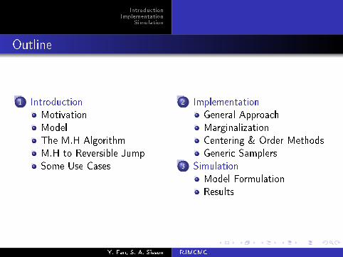
Outline
1 Introduction
Motivation
Model
The M.H Algorithm
M.H to Reversible Jump
Some Use Cases
2 Implementation
General Approach
Marginalization
Centering & Order Methods
Generic Samplers3 Simulation
Model Formulation
Results
Y. Fan, S. A. Sisson RJMCMC

IntroductionImplementation
Simulation
MotivationModelThe M.H AlgorithmM.H to Reversible JumpSome Use Cases
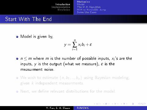
Start With The End
Model is given by,
y =n
∑i=1
xibi + ε
n ≤m where m is the number of possible inputs, xi 's are the
inputs, y is the output (what we measure), ε is the
measurment noise.
We wish to estimate {n,b1, ..,bn} using Bayesian modeling,
given k independent measurments.
Next, we de�ne relevant distributions for the model.
Y. Fan, S. A. Sisson RJMCMC
IntroductionImplementation
Simulation
MotivationModelThe M.H AlgorithmM.H to Reversible JumpSome Use Cases
Start With The End
Model is given by,
y =n
∑i=1
xibi + ε
n ≤m where m is the number of possible inputs, xi 's are the
inputs, y is the output (what we measure), ε is the
measurment noise.
We wish to estimate {n,b1, ..,bn} using Bayesian modeling,
given k independent measurments.
Next, we de�ne relevant distributions for the model.
Y. Fan, S. A. Sisson RJMCMC
IntroductionImplementation
Simulation
MotivationModelThe M.H AlgorithmM.H to Reversible JumpSome Use Cases
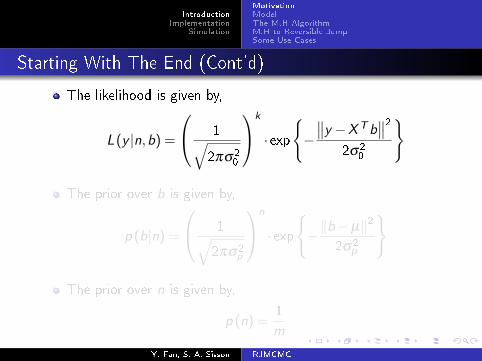
Starting With The End (Cont'd)
The likelihood is given by,
L(y |n,b) =
1√2πσ2
0
k
· exp
{−∥∥y −XTb
∥∥22σ2
0
}
The prior over b is given by,
p (b|n) =
1√2πσ2
p
n
· exp
{−‖b−µ‖2
2σ2p
}
The prior over n is given by,
p (n) =1
m
Y. Fan, S. A. Sisson RJMCMC

IntroductionImplementation
Simulation
MotivationModelThe M.H AlgorithmM.H to Reversible JumpSome Use Cases
Outline
1 Introduction
Motivation
Model
The M.H Algorithm
M.H to Reversible Jump
Some Use Cases
2 Implementation
General Approach
Marginalization
Centering & Order Methods
Generic Samplers3 Simulation
Model Formulation
Results
Y. Fan, S. A. Sisson RJMCMC
IntroductionImplementation
Simulation
MotivationModelThe M.H AlgorithmM.H to Reversible JumpSome Use Cases
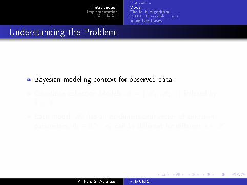
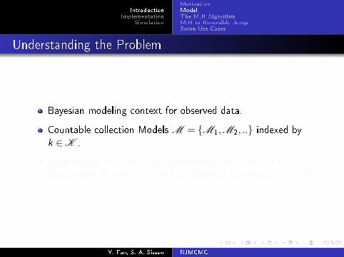
Understanding the Problem
Bayesian modeling context for observed data.
Countable collection Models M = {M1,M2, ..} indexed by
k ∈K .
Each model Mk has an nk -dimensional vector of unknown
parameters, θk ∈ Rnk . nk can be di�erent for di�erent k ∈K .
Y. Fan, S. A. Sisson RJMCMC
IntroductionImplementation
Simulation
MotivationModelThe M.H AlgorithmM.H to Reversible JumpSome Use Cases
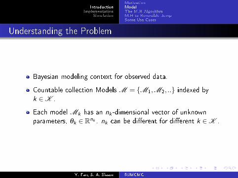
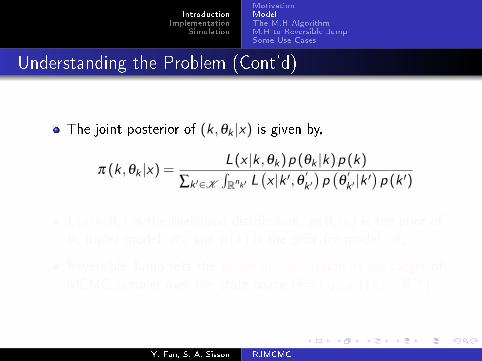
Understanding the Problem (Cont'd)
The joint posterior of (k ,θk |x) is given by,
π (k ,θk |x) =L(x |k,θk)p (θk |k)p (k)
∑k ′∈K∫Rnk ′ L
(x |k ′,θ ′k ′
)p(θ′k ′ |k ′
)p (k ′)
L(x |k,θk) is the likelihood distribution, p (θk |k) is the prior of
θk under model Mk and p (k) is the prior for model Mk .
Reversible Jump sets the posterior distribution as the target of
MCMC sampler over the state space Θ = ∪k∈K ({k}×Rnk ).
Y. Fan, S. A. Sisson RJMCMC
IntroductionImplementation
Simulation
MotivationModelThe M.H AlgorithmM.H to Reversible JumpSome Use Cases
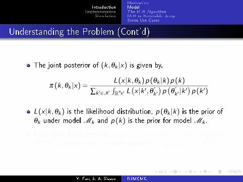
Understanding the Problem (Cont'd)
The joint posterior of (k ,θk |x) is given by,
π (k ,θk |x) =L(x |k,θk)p (θk |k)p (k)
∑k ′∈K∫Rnk ′ L
(x |k ′,θ ′k ′
)p(θ′k ′ |k ′
)p (k ′)
L(x |k,θk) is the likelihood distribution, p (θk |k) is the prior of
θk under model Mk and p (k) is the prior for model Mk .
Reversible Jump sets the posterior distribution as the target of
MCMC sampler over the state space Θ = ∪k∈K ({k}×Rnk ).
Y. Fan, S. A. Sisson RJMCMC

IntroductionImplementation
Simulation
MotivationModelThe M.H AlgorithmM.H to Reversible JumpSome Use Cases
Outline
1 Introduction
Motivation
Model
The M.H Algorithm
M.H to Reversible Jump
Some Use Cases
2 Implementation
General Approach
Marginalization
Centering & Order Methods
Generic Samplers3 Simulation
Model Formulation
Results
Y. Fan, S. A. Sisson RJMCMC

IntroductionImplementation
Simulation
MotivationModelThe M.H AlgorithmM.H to Reversible JumpSome Use Cases
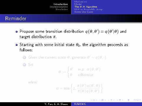
Reminder
Propose some transition distribution q (θ ,θ ′)≡ q (θ ′|θ) and
target distribution π.
Starting with some initial state θ0, the algorithm proceeds as
follows:
1 Given the current state θ , generate θ ′ ∼ q (θ , ·).
2 Set
θ :=
{θ ′ w.p. α (θ ,θ ′)
θ otherwise
where
α = min
{1,
π (θ ′)q (θ ′,θ)
π (θ)q (θ ,θ ′)
}
Y. Fan, S. A. Sisson RJMCMC
IntroductionImplementation
Simulation
MotivationModelThe M.H AlgorithmM.H to Reversible JumpSome Use Cases
Reminder
Propose some transition distribution q (θ ,θ ′)≡ q (θ ′|θ) and
target distribution π.
Starting with some initial state θ0, the algorithm proceeds as
follows:
1 Given the current state θ , generate θ ′ ∼ q (θ , ·).
2 Set
θ :=
{θ ′ w.p. α (θ ,θ ′)
θ otherwise
where
α = min
{1,
π (θ ′)q (θ ′,θ)
π (θ)q (θ ,θ ′)
}
Y. Fan, S. A. Sisson RJMCMC

IntroductionImplementation
Simulation
MotivationModelThe M.H AlgorithmM.H to Reversible JumpSome Use Cases
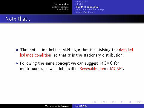
Note that..
The motivation behind M.H algorithm is satisfying the detailed
balance condition, so that π is the stationary distribution.
Following the same concept we can suggest MCMC for
multi-models as well, let's call it Reversible Jump MCMC.
Y. Fan, S. A. Sisson RJMCMC
IntroductionImplementation
Simulation
MotivationModelThe M.H AlgorithmM.H to Reversible JumpSome Use Cases
Outline
1 Introduction
Motivation
Model
The M.H Algorithm
M.H to Reversible Jump
Some Use Cases
2 Implementation
General Approach
Marginalization
Centering & Order Methods
Generic Samplers3 Simulation
Model Formulation
Results
Y. Fan, S. A. Sisson RJMCMC

IntroductionImplementation
Simulation
MotivationModelThe M.H AlgorithmM.H to Reversible JumpSome Use Cases
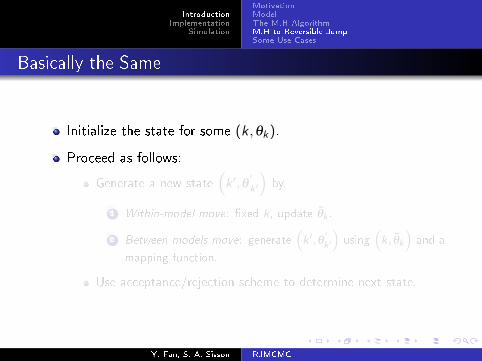
Basically the Same
Initialize the state for some (k ,θk).
Proceed as follows:
Generate a new state(k ′,θ
′k ′
)by,
1 Within-model move: �xed k, update θ̃k .
2 Between-models move: generate(k ′,θ
′
k ′
)using
(k, θ̃k
)and a
mapping function.
Use acceptance/rejection scheme to determine next state.
Y. Fan, S. A. Sisson RJMCMC
IntroductionImplementation
Simulation
MotivationModelThe M.H AlgorithmM.H to Reversible JumpSome Use Cases
Basically the Same
Initialize the state for some (k ,θk).
Proceed as follows:
Generate a new state(k ′,θ
′k ′
)by,
1 Within-model move: �xed k, update θ̃k .
2 Between-models move: generate(k ′,θ
′
k ′
)using
(k, θ̃k
)and a
mapping function.
Use acceptance/rejection scheme to determine next state.
Y. Fan, S. A. Sisson RJMCMC

IntroductionImplementation
Simulation
MotivationModelThe M.H AlgorithmM.H to Reversible JumpSome Use Cases
Outline
1 Introduction
Motivation
Model
The M.H Algorithm
M.H to Reversible Jump
Some Use Cases
2 Implementation
General Approach
Marginalization
Centering & Order Methods
Generic Samplers3 Simulation
Model Formulation
Results
Y. Fan, S. A. Sisson RJMCMC

IntroductionImplementation
Simulation
MotivationModelThe M.H AlgorithmM.H to Reversible JumpSome Use Cases
Examples Time
Finite Mixture Models
Model is in the form
f (x |θk) =k
∑j=1
ωj fj (x |φj)
where θk = (φ1, ..,φk), ∑kj=1
ωj = 1, and the number of mixture
models, k , is also unknown.
Y. Fan, S. A. Sisson RJMCMC

IntroductionImplementation
Simulation
MotivationModelThe M.H AlgorithmM.H to Reversible JumpSome Use Cases
Examples Time (Cont'd)
Variable Selection
Model is in the form
Y = Xγβγ + ε
where γ is a binary vector indexing the subset of X to be included,
β are the regression coe�cients and ε is noise.
Y. Fan, S. A. Sisson RJMCMC
IntroductionImplementation
Simulation
MotivationModelThe M.H AlgorithmM.H to Reversible JumpSome Use Cases
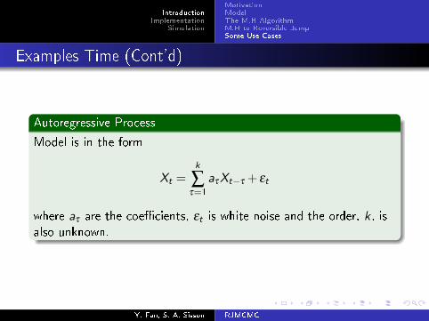
Examples Time (Cont'd)
Autoregressive Process
Model is in the form
Xt =k
∑τ=1
aτXt−τ + εt
where aτ are the coe�cients, εt is white noise and the order, k , isalso unknown.
Y. Fan, S. A. Sisson RJMCMC
IntroductionImplementation
Simulation
General ApproachMarginalizationCentering & Order MethodsGeneric Samplers
Outline
1 Introduction
Motivation
Model
The M.H Algorithm
M.H to Reversible Jump
Some Use Cases
2 Implementation
General Approach
Marginalization
Centering & Order Methods
Generic Samplers3 Simulation
Model Formulation
Results
Y. Fan, S. A. Sisson RJMCMC
IntroductionImplementation
Simulation
General ApproachMarginalizationCentering & Order MethodsGeneric Samplers
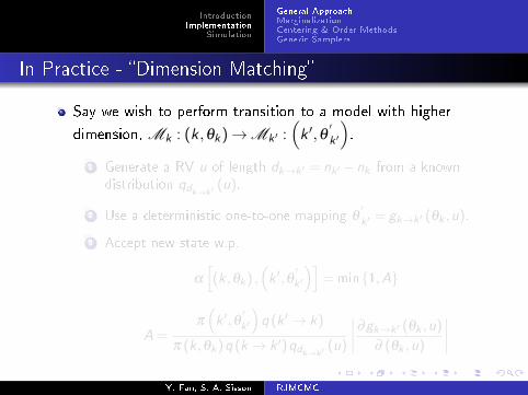
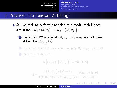
In Practice - �Dimension Matching�
Say we wish to perform transition to a model with higher
dimension, Mk : (k ,θk)→Mk ′ :(k ′,θ
′
k ′
).
1 Generate a RV u of length dk→k ′ = nk ′ −nk from a knowndistribution qdk→k ′
(u).
2 Use a deterministic one-to-one mapping θ′k ′ = gk→k ′ (θk ,u).
3 Accept new state w.p.
α
[(k ,θk) ,
(k ′,θ
′k ′
)]= min{1,A}
A =π
(k ′,θ
′k ′
)q (k ′→ k)
π (k ,θk)q (k → k ′)qdk→k ′(u)
∣∣∣∣∂gk→k ′ (θk ,u)
∂ (θk ,u)
∣∣∣∣Y. Fan, S. A. Sisson RJMCMC
IntroductionImplementation
Simulation
General ApproachMarginalizationCentering & Order MethodsGeneric Samplers
In Practice - �Dimension Matching�
Say we wish to perform transition to a model with higher
dimension, Mk : (k ,θk)→Mk ′ :(k ′,θ
′
k ′
).
1 Generate a RV u of length dk→k ′ = nk ′ −nk from a knowndistribution qdk→k ′
(u).
2 Use a deterministic one-to-one mapping θ′k ′ = gk→k ′ (θk ,u).
3 Accept new state w.p.
α
[(k ,θk) ,
(k ′,θ
′k ′
)]= min{1,A}
A =π
(k ′,θ
′k ′
)q (k ′→ k)
π (k ,θk)q (k → k ′)qdk→k ′(u)
∣∣∣∣∂gk→k ′ (θk ,u)
∂ (θk ,u)
∣∣∣∣Y. Fan, S. A. Sisson RJMCMC
IntroductionImplementation
Simulation
General ApproachMarginalizationCentering & Order MethodsGeneric Samplers
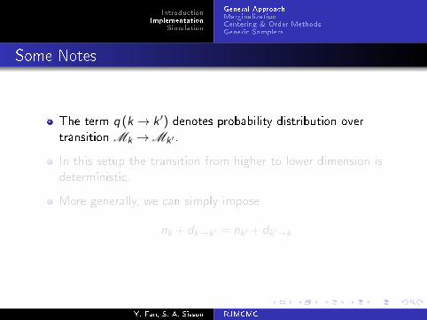
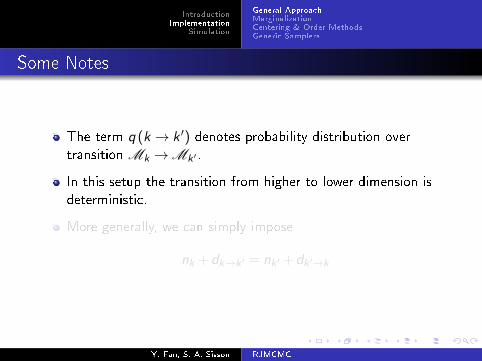
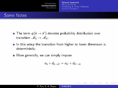
Some Notes
The term q (k → k ′) denotes probability distribution over
transition Mk →Mk ′ .
In this setup the transition from higher to lower dimension is
deterministic.
More generally, we can simply impose
nk +dk→k ′ = nk ′ +dk ′→k
Y. Fan, S. A. Sisson RJMCMC
IntroductionImplementation
Simulation
General ApproachMarginalizationCentering & Order MethodsGeneric Samplers
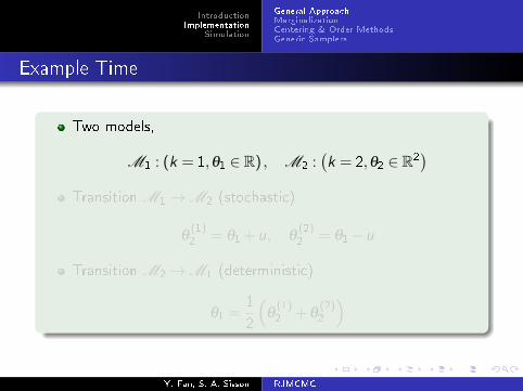
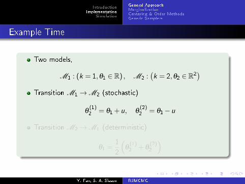
Example Time
Two models,
M1 : (k = 1,θ1 ∈ R) , M2 :(k = 2,θ2 ∈ R2
)Transition M1→M2 (stochastic)
θ(1)2
= θ1 +u, θ(2)2
= θ1−u
Transition M2→M1 (deterministic)
θ1 =1
2
(θ(1)2
+ θ(2)2
)
Y. Fan, S. A. Sisson RJMCMC
IntroductionImplementation
Simulation
General ApproachMarginalizationCentering & Order MethodsGeneric Samplers
Example Time
Two models,
M1 : (k = 1,θ1 ∈ R) , M2 :(k = 2,θ2 ∈ R2
)Transition M1→M2 (stochastic)
θ(1)2
= θ1 +u, θ(2)2
= θ1−u
Transition M2→M1 (deterministic)
θ1 =1
2
(θ(1)2
+ θ(2)2
)
Y. Fan, S. A. Sisson RJMCMC
IntroductionImplementation
Simulation
General ApproachMarginalizationCentering & Order MethodsGeneric Samplers
Outline
1 Introduction
Motivation
Model
The M.H Algorithm
M.H to Reversible Jump
Some Use Cases
2 Implementation
General Approach
Marginalization
Centering & Order Methods
Generic Samplers3 Simulation
Model Formulation
Results
Y. Fan, S. A. Sisson RJMCMC
IntroductionImplementation
Simulation
General ApproachMarginalizationCentering & Order MethodsGeneric Samplers
Making Life Easier
In some Bayesian models, integrating over all (or parts of) θk
is possible.
Usually arises when assuming some structures such as
conjugate priors.
Results in smaller state space, thus often easier to implement.
Y. Fan, S. A. Sisson RJMCMC
IntroductionImplementation
Simulation
General ApproachMarginalizationCentering & Order MethodsGeneric Samplers
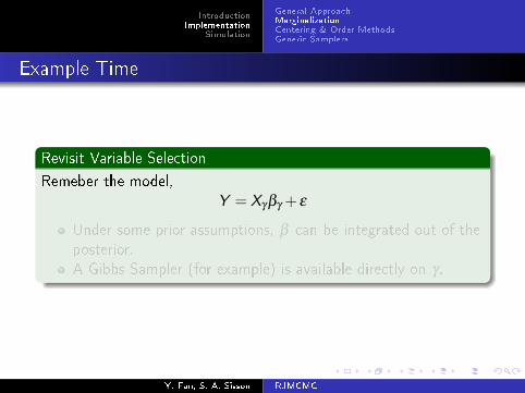
Example Time
Revisit Variable Selection
Remeber the model,
Y = Xγβγ + ε
Under some prior assumptions, β can be integrated out of the
posterior.
A Gibbs Sampler (for example) is available directly on γ .
Y. Fan, S. A. Sisson RJMCMC

IntroductionImplementation
Simulation
General ApproachMarginalizationCentering & Order MethodsGeneric Samplers
Example Time
Revisit Variable Selection
Remeber the model,
Y = Xγβγ + ε
Under some prior assumptions, β can be integrated out of the
posterior.
A Gibbs Sampler (for example) is available directly on γ .
Y. Fan, S. A. Sisson RJMCMC
IntroductionImplementation
Simulation
General ApproachMarginalizationCentering & Order MethodsGeneric Samplers
Outline
1 Introduction
Motivation
Model
The M.H Algorithm
M.H to Reversible Jump
Some Use Cases
2 Implementation
General Approach
Marginalization
Centering & Order Methods
Generic Samplers3 Simulation
Model Formulation
Results
Y. Fan, S. A. Sisson RJMCMC
IntroductionImplementation
Simulation
General ApproachMarginalizationCentering & Order MethodsGeneric Samplers
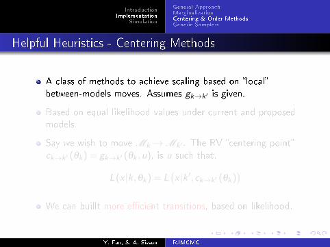
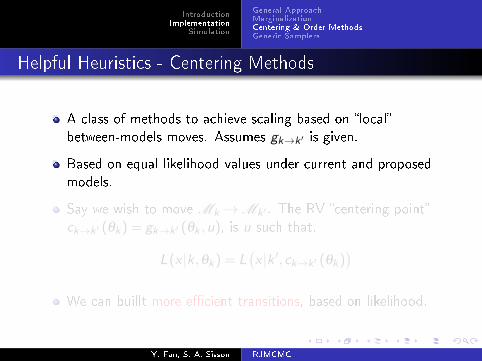
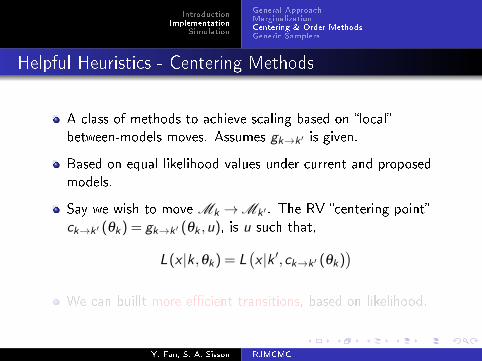
Helpful Heuristics - Centering Methods
A class of methods to achieve scaling based on �local�
between-models moves. Assumes gk→k ′ is given.
Based on equal likelihood values under current and proposed
models.
Say we wish to move Mk →Mk ′ . The RV �centering point�
ck→k ′ (θk) = gk→k ′ (θk ,u), is u such that,
L(x |k ,θk) = L(x |k ′,ck→k ′ (θk)
)We can buillt more e�cient transitions, based on likelihood.
Y. Fan, S. A. Sisson RJMCMC
IntroductionImplementation
Simulation
General ApproachMarginalizationCentering & Order MethodsGeneric Samplers
Helpful Heuristics - Centering Methods
A class of methods to achieve scaling based on �local�
between-models moves. Assumes gk→k ′ is given.
Based on equal likelihood values under current and proposed
models.
Say we wish to move Mk →Mk ′ . The RV �centering point�
ck→k ′ (θk) = gk→k ′ (θk ,u), is u such that,
L(x |k ,θk) = L(x |k ′,ck→k ′ (θk)
)We can buillt more e�cient transitions, based on likelihood.
Y. Fan, S. A. Sisson RJMCMC

IntroductionImplementation
Simulation
General ApproachMarginalizationCentering & Order MethodsGeneric Samplers
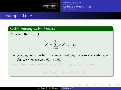
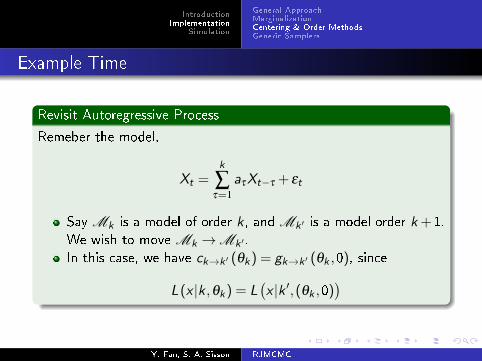
Example Time
Revisit Autoregressive Process
Remeber the model,
Xt =k
∑τ=1
aτXt−τ + εt
Say Mk is a model of order k , and Mk ′ is a model order k +1.
We wish to move Mk →Mk ′ .
In this case, we have ck→k ′ (θk) = gk→k ′ (θk ,0), since
L(x |k ,θk) = L(x |k ′,(θk ,0)
)
Y. Fan, S. A. Sisson RJMCMC
IntroductionImplementation
Simulation
General ApproachMarginalizationCentering & Order MethodsGeneric Samplers
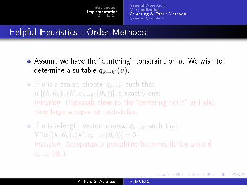
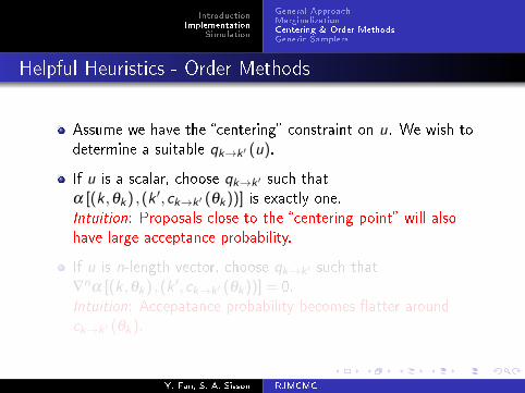
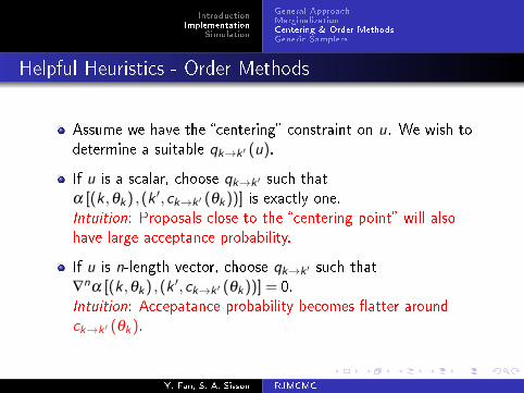
Helpful Heuristics - Order Methods
Assume we have the �centering� constraint on u. We wish to
determine a suitable qk→k ′ (u).
If u is a scalar, choose qk→k ′ such that
α [(k,θk) ,(k ′,ck→k ′ (θk))] is exactly one.
Intuition: Proposals close to the �centering point� will also
have large acceptance probability.
If u is n-length vector, choose qk→k ′ such that
∇nα [(k ,θk) ,(k ′,ck→k ′ (θk))] = 0.
Intuition: Accepatance probability becomes �atter around
ck→k ′ (θk).
Y. Fan, S. A. Sisson RJMCMC
IntroductionImplementation
Simulation
General ApproachMarginalizationCentering & Order MethodsGeneric Samplers
Helpful Heuristics - Order Methods
Assume we have the �centering� constraint on u. We wish to
determine a suitable qk→k ′ (u).
If u is a scalar, choose qk→k ′ such that
α [(k,θk) ,(k ′,ck→k ′ (θk))] is exactly one.
Intuition: Proposals close to the �centering point� will also
have large acceptance probability.
If u is n-length vector, choose qk→k ′ such that
∇nα [(k ,θk) ,(k ′,ck→k ′ (θk))] = 0.
Intuition: Accepatance probability becomes �atter around
ck→k ′ (θk).
Y. Fan, S. A. Sisson RJMCMC

IntroductionImplementation
Simulation
General ApproachMarginalizationCentering & Order MethodsGeneric Samplers
Outline
1 Introduction
Motivation
Model
The M.H Algorithm
M.H to Reversible Jump
Some Use Cases
2 Implementation
General Approach
Marginalization
Centering & Order Methods
Generic Samplers3 Simulation
Model Formulation
Results
Y. Fan, S. A. Sisson RJMCMC

IntroductionImplementation
Simulation
General ApproachMarginalizationCentering & Order MethodsGeneric Samplers
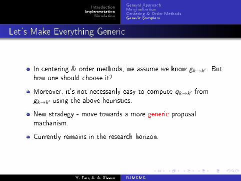
Let's Make Everything Generic
In centering & order methods, we assume we know gk→k ′ . But
how one should choose it?
Moreover, it's not necessarily easy to compute qk→k ′ from
gk→k ′ using the above heuristics.
New stradegy - move towards a more generic proposal
machanism.
Currently remains in the research horizon.
Y. Fan, S. A. Sisson RJMCMC

IntroductionImplementation
Simulation
General ApproachMarginalizationCentering & Order MethodsGeneric Samplers
Let's Make Everything Generic
In centering & order methods, we assume we know gk→k ′ . But
how one should choose it?
Moreover, it's not necessarily easy to compute qk→k ′ from
gk→k ′ using the above heuristics.
New stradegy - move towards a more generic proposal
machanism.
Currently remains in the research horizon.
Y. Fan, S. A. Sisson RJMCMC

IntroductionImplementation
Simulation
General ApproachMarginalizationCentering & Order MethodsGeneric Samplers
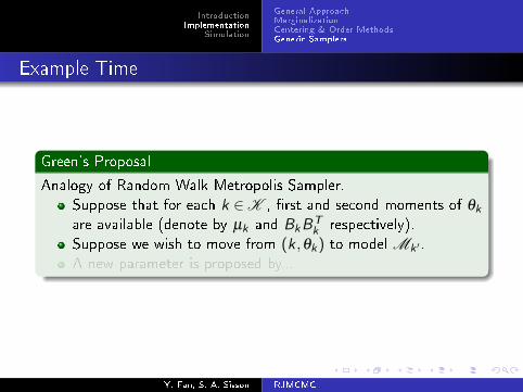
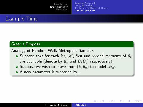
Example Time
Green's Proposal
Analogy of Random-Walk Metropolis Sampler.
Suppose that for each k ∈K , �rst and second moments of θk
are available (denote by µk and BkBTk respectively).
Suppose we wish to move from (k ,θk) to model Mk ′ .
A new parameter is proposed by...
Y. Fan, S. A. Sisson RJMCMC

IntroductionImplementation
Simulation
General ApproachMarginalizationCentering & Order MethodsGeneric Samplers
Example Time
Green's Proposal
Analogy of Random-Walk Metropolis Sampler.
Suppose that for each k ∈K , �rst and second moments of θk
are available (denote by µk and BkBTk respectively).
Suppose we wish to move from (k ,θk) to model Mk ′ .
A new parameter is proposed by...
Y. Fan, S. A. Sisson RJMCMC

IntroductionImplementation
Simulation
General ApproachMarginalizationCentering & Order MethodsGeneric Samplers
Example Time (Cont'd)
Green's Proposal
θ′
k ′ =
µk ′ +Bk ′
[RB−1k (θk −µk)
]nk ′1
if nk ′ < nk
µk ′ +Bk ′RB−1k (θk −µk) if nk ′ = nk
µk ′ +Bk ′R
(B−1k (θk −µk)
u
)if nk ′ > nk
where [·]m1denotes the �rst m componenets, R �xed orthogonal
matrix of order max{nk ,nk ′}, and u ∼ qnk ′−nk (u).
Y. Fan, S. A. Sisson RJMCMC
IntroductionImplementation
Simulation
Model FormulationResults
Outline
1 Introduction
Motivation
Model
The M.H Algorithm
M.H to Reversible Jump
Some Use Cases
2 Implementation
General Approach
Marginalization
Centering & Order Methods
Generic Samplers3 Simulation
Model Formulation
Results
Y. Fan, S. A. Sisson RJMCMC

IntroductionImplementation
Simulation
Model FormulationResults
Setting Up The Model
Model is given by,
y =n
∑i=1
xibi + ε
n≤m where m is the number of predictors, xi 's are the inputs,y is the output (what we measure), ε is the measurment noise.
We wish to estimate {n,b1, ..,bn} using Bayesian modeling,
given k independent measurments.
Next, we de�ne relevant distributions.
Y. Fan, S. A. Sisson RJMCMC
IntroductionImplementation
Simulation
Model FormulationResults
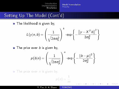
Setting Up The Model (Cont'd)
The likelihood is given by,
L(y |n,b) =
1√2πσ2
0
k
· exp
{−∥∥y −XTb
∥∥22σ2
0
}
The prior over b is given by,
p (b|n) =
1√2πσ2
p
n
· exp
{−‖b−µ‖2
2σ2p
}
The prior over n is given by,
p (n) =1
m
Y. Fan, S. A. Sisson RJMCMC
IntroductionImplementation
Simulation
Model FormulationResults
Setting Up The Model (Cont'd)
The likelihood is given by,
L(y |n,b) =
1√2πσ2
0
k
· exp
{−∥∥y −XTb
∥∥22σ2
0
}
The prior over b is given by,
p (b|n) =
1√2πσ2
p
n
· exp
{−‖b−µ‖2
2σ2p
}
The prior over n is given by,
p (n) =1
m
Y. Fan, S. A. Sisson RJMCMC

IntroductionImplementation
Simulation
Model FormulationResults
Outline
1 Introduction
Motivation
Model
The M.H Algorithm
M.H to Reversible Jump
Some Use Cases
2 Implementation
General Approach
Marginalization
Centering & Order Methods
Generic Samplers3 Simulation
Model Formulation
Results
Y. Fan, S. A. Sisson RJMCMC
IntroductionImplementation
Simulation
Model FormulationResults
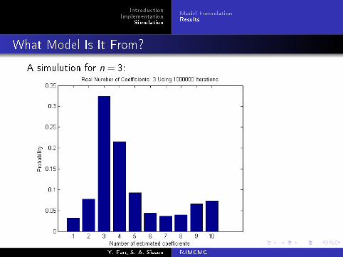
What Model Is It From?
A simulution for n = 3:
Y. Fan, S. A. Sisson RJMCMC

IntroductionImplementation
Simulation
Model FormulationResults
What Model Is It From?
A simulution for n = 7:
Y. Fan, S. A. Sisson RJMCMC

IntroductionImplementation
Simulation
Model FormulationResults
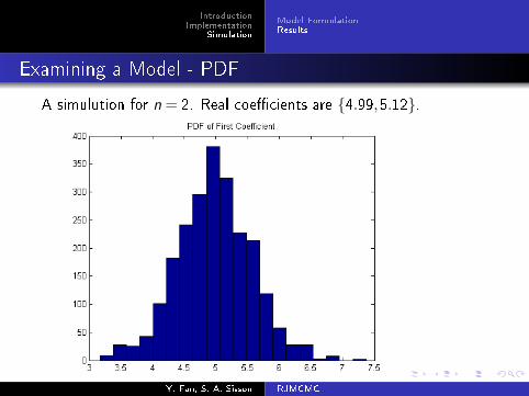
Examining a Model - PDF
A simulution for n = 2. Real coe�cients are {4.99,5.12}.�Clutter� - State Space Samples.
Y. Fan, S. A. Sisson RJMCMC
IntroductionImplementation
Simulation
Model FormulationResults
Examining a Model - PDF
A simulution for n = 2. Real coe�cients are {4.99,5.12}.
Y. Fan, S. A. Sisson RJMCMC
IntroductionImplementation
Simulation
Model FormulationResults
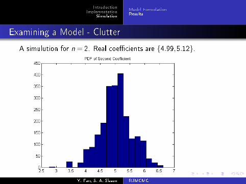
Examining a Model - Clutter
A simulution for n = 2. Real coe�cients are {4.99,5.12}.
Y. Fan, S. A. Sisson RJMCMC