Signal Sapce Representation

Chapter: 5 Signal Space

Representation

1

Concept of orthogonality and orthonormalityLet fm(x) and fn(x) be two real valued

functions defined over the interval a ≤ x ≤ b.

If the product [fm(x)×fn(x)] exists over the interval, the two functions are called orthogonal to each other in the interval a ≤x≤ b when the following condition holds:

• A set of real valued functions f1(x), f2(x)…fN(x) is called an orthogonal set over an interval a ≤ x ≤ b if

(i) all the functions exist in that interval and

(ii) all distinct pairs of the functions are orthogonal to each other over the interval, i.e.

Concept of orthogonality and orthonormality

• An orthogonal set of functions f1(x), f2(x)… fN(x) is called an orthonormal set if,

• An orthonormal set can be obtained from a corresponding orthogonal set of functions by dividing each function by its norm.

concept of orthogonality and orthonormality

Now, let us consider a set of real functions f1(x), f2(x)… fN(x) such that, for some non-negative weight function w(x) over the interval a ≤ x ≤ b

an orthogonal set with respect to the weight function w(x) over the interval a ≤ x ≤ b by defining the norm as,

concept of orthogonality and orthonormality

an orthogonal set of gi -s can be used to get an orthogonal set of fi-s with respect to a specific non-negative weight function w(x) over a ≤ x ≤ b by the following substitution (provided √w(x)≠0, a ≤ x ≤ b):

A real orthogonal set can be generated by using the concepts of Strum-Liouville (S-L) equation.


• It satisfies the following boundary conditions:

• Here c1, c2, d1 and d2 are real constants such that at least one of c1 and c2 is non zero and at least one of d1 and d2 is non zero.

7


• The Strum-Livouille equation,

• Let the functions p(x), q(x) and ω(x) be real valued and continuous in the interval a ≤ x ≤ b.

• Let ym(x) and yn(x) be eigen functions of the S-L problem corresponding to distinct eigenvalues λm and λn respectively.

• ym(x) and yn(x) are orthogonal over a ≤ x ≤ b with respect to the weight function w(x).

8

Orthogonality Theorem

if p(x =a) = 0, and if p(x = b) = 0, then boundary condition (i) and (ii) may be omitted from the problem. If p(x = a) = p(x = b), then the boundary condition can be simplified as,

• We know that, for integer ‘m’ and ‘n’, • (1)

• by substituting x = 2πft = ω t and dx = 2πfdt = ω dt equation (1) can be written as,

• (2)

10

Example of Orthogonal Sets:

• equation (2) is orthogonal in terms of the independent variable ‘t’ over the fundamental range 1/f and, in general, over M.1/f = M.T0,

• where ‘T0’ indicates the fundamental time interval over which cos2πmft and cos2πnft are orthogonal to each other.

• if two cosine signals have a frequency difference ‘f’, then we may say,

11

Example of Orthogonal Sets (Cont.):

• where mf = (n+p)f and ‘p’ is an integer.

12


• Let us define,•

• we use the above observations on orthogonality to distinguish among ‘si-s’ over a decision interval of T5 = T0 =1/f

13


Importance of the Concepts of Orthogonality in Digital

Communicationsa. In the design and selection of information bearing pulses, orthogonality over a symbol duration may be used to advantage for deriving efficient symbol-by-symbol demodulation scheme.

b. Performance analysis of several modulation demodulation schemes can be carried out if the information-bearing signal waveforms are known to be orthogonal to each other.

c. The concepts of orthogonality can be used to advantage in the design and selection of single and multiple carriers for modulation, transmission and reception.

Orthogonality in a complex domain

• Let us consider a complex function,

• We know that cosθ & sinθ are orthogonal to each other over -π ≤ θ < π , i.e.,

Orthogonality in a complex domain

• So, using a constant weight function w = r, which is non-negative, we may say

• Now, x = r cos θ and y = r sin θ are also orthogonal over -π ≤ θ < π.

• Now, let ‘θ’ be a continuous function of ‘t’ over -π ≤ θ < π. And,

• Assuming a linear relationship, let,

17

• Under these conditions, we see,

• i.e., x(t) and y(t) are orthogonal over the interval

Gram Schmitz Orthogonalization

• The GSO states that any set of M energy signals, {si(t)}, 1 ≤ i ≤ M can be expressed as linear combinations of N orthonormal basis functions, where N ≤ M. If s1(t), s2(t), ….., sM(t) are real valued energy signals, each of duration ‘T’ sec,

(1)

(2)

The ϕj(t)-s are the basis functions and ‘sij’-s are scalar coefficients.

Gram-Schmidt Orthogonalization (GSO)

• The GSO states that any set of M energy signals, {si(t)}, 1 ≤ i ≤ M can be expressed as linear combinations of N orthonormal basis functions, where N ≤ M. If s1(t), s2(t), ….., sM(t) are real valued energy signals, each of duration ‘T’ sec,

(1)

(2)

The ϕj(t)-s are the basis functions and ‘sij’-s are scalar coefficients.

• We will consider real-valued basis functions ϕj(t) - s which are orthonormal to each other, i.e.,

• Note that each basis function has unit energy over the symbol duration ‘T’.

Justification for G-S-O procedure

• Any given set of energy signals, {si(t)}, 1 ≤ i ≤ M over 0 ≤ t < T, can be completely described by a subset of energy signals whose elements are linearly independent.

• let us assume that all si(t)-s are not linearly independent. Then, there must exist a set of coefficients {ai}, 1 < i ≤ M, not all of which are zero,

• a1 ≠ 0 and a3 ≠ 0, then s1(t) and s3(t) are dependent signals.

24

Let us arbitrarily set, aM ≠ 0. Then,

The set may be either linearly independent or not. If not, there exists a set of {bi}, i = 1,2…, (M – 1), not all equal to zero such that,

Again, arbitrarily assuming that bM-1≠ 0, we may express sM-1(t) as,

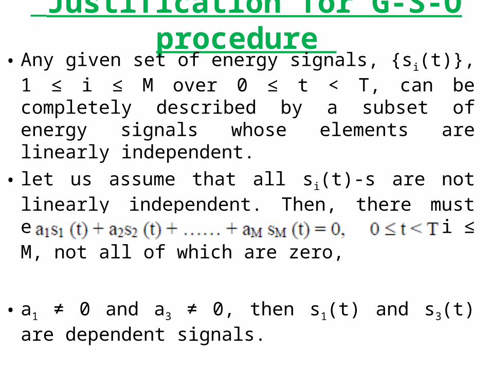
Justification for G-S-O procedure (Part-2)

• We now show that it is possible to construct a set of ‘N’ orthonormal basis functions ϕ1(t), ϕ2(t), ….., ϕN(t) from {si(t)}, i = 1, 2, ….., N.

• first basis function as, ϕ1(t) and E1 denotes the energy of the first signal s1(t),


• So, we verified that the function g2(t) is orthogonal to the first basis function. This gives us a clue to determine the second basis function.

• Now, energy of g2(t),

we can determine the third basis function, ϕ3(t). For i=3,

Indeed, in general,

for i = 1, 2,….., N, where

for i = 1, 2,….., N and j = 1, 2, …, M

Summary of Gram-Schmidt Orthogonalization Method

• If the signal set {sj(t)} is known for j = 1,2,….., M, 0 ≤ t <T,

• Derive a subset of linearly independent energy signals, {si(t)},i = 1, 2,….., N ≤ M.

• Find the energy of s1(t) as this energy helps in determining the first basis function ϕ1(t), which is a normalized form of the first signal. Note that the choice of this ‘first’ signal is arbitrary.

• Find the scalar ‘s21’, energy of the second signal (E2), a special function ‘g2(t)’ which is orthogonal to the first basis function and then finally the second orthonormal basis function ϕ2(t)

• Follow the same procedure as that of finding the second basis function to obtain the other basis functions. 30

Example:1 (a) Use the Gram-Schmidt procedure to find a set orthonormal basis functions corresponding to the signals show below.

(a)Express x1, x2, and x3 in terms of the orthonormal basis functions found in part 1)

Solution: Step 1:

31

Step 2:

Step 3:

32

Concept of Signal Space • Let, for a convenient set of {ϕj (t)}, j =

1,2,…,N and 0 ≤ t <T,

• Now, we can represent a signal si(t) as a column vector whose elements are the scalar coefficients sij, j = 1, 2, ….., N :

Concept of Signal Space • These M energy signals or vectors can

be viewed as a set of M points in an N – dimensional Euclidean space, known as the ‘Signal Space’

• Signal Constellation is the collection of M signals points (or messages) on the signal space.

Sketch of a 2-dimentional-signal space showing three signal vectors

Concept of Signal Space

• The squared norm is the inner product of the vector

• The cosine of the angle between two vectors is defined as,

• If Ei is the energy of the i-th signal vector,

Schwarz Inequality• According to Schwarz inequality states that the

pair of energy signals S1(t) and S2(t) holds the relationship,

• If and only if S2(t) = C.S1(t) where C is any constant.

Proof:- S1(t) and S2(t) expressed in terms of their orthonormal basis functions and

• Where and satisfy the orthonormality condition over the interval (-∞ ∞)

dttSdttSdttStS )()()()( 22

21

2

21

)(2 t)(1 t

)()()()()()(

2221212

2121111

tStStStStStS

elsewherejifor

dttt ij 0 1

)()( 21

)(2 t)(1 t

Schwarz Inequality cont.• The signals S1(t) and S2(t) reprsented by the respective

pair of vectors,

The angle subtended between the vector S1 and S2 is,

This verifies the Schwarz inequality.

22

212

12

111

SS

SandSS

S

21

21

SSSSCos

T

2/1

22

2/1

21

21

)()(

)()(

dttSdttS

dttStSCos

1Cos

Schwarz Inequality cont.• If the signals S1(t) and S2(t) reprsented by the

complex real valued signal then equation may be represented as,

• Where the equality holds if and only if S2(t) = C.S1(t) where C is the constant.

dttSdttSdttStS2

2

2

1

2

*1 )()()()(

2

Signal Sapce Representation

Documents

Transcript of Signal Sapce Representation