SigmaXL Version 6.1 Workbook · PDF fileSigmaXL® Version 6.1 Workbook. ... Process Sigma...
320
Copyright © 2004-2011, SigmaXL Inc. SigmaXL ® Version 6.1 Workbook Contact Information: Technical Support: 1-866-475-2124 (Toll Free in North America) or 1-416-236-5877 Sales: 1-888-SigmaXL (888-744-6295) E-mail: [email protected] Web: www.SigmaXL.com
Transcript of SigmaXL Version 6.1 Workbook · PDF fileSigmaXL® Version 6.1 Workbook. ... Process Sigma...
Copyright © 2004-2011, SigmaXL Inc.
SigmaXL® Version 6.1
Workbook Contact Information:
Technical Support: 1-866-475-2124 (Toll Free in North America) or 1-416-236-5877
Sales: 1-888-SigmaXL (888-744-6295)
E-mail: [email protected] Web: www.SigmaXL.com

iii
Table of Contents
SigmaXL® Feature List Summary, What’s New in Version 6.0 & 6.1, Installation Notes, System Requirements and Getting Help..................................................................................11
SigmaXL Version 6.1 Feature List Summary..............................................................................13
What’s New in Versions 6.0 & 6.1 ..............................................................................................15
Installation Notes .........................................................................................................................18
Activation via the Internet: ....................................................................................................21
Error Messages: .....................................................................................................................23
Activation via E-Mail or Telephone: .....................................................................................24
Installation Notes for Excel 2007/2010 .......................................................................................27
SigmaXL® Defaults and Menu Options.......................................................................................29
Clear Saved Defaults..............................................................................................................29
Data Selection Default ...........................................................................................................29
Menu Options (Classical or DMAIC)....................................................................................30
SigmaXL® System Requirements ................................................................................................31
Getting Help and Product Registration ........................................................................................32
Introduction to SigmaXL® Data Format and Tools Summary ............................................33
Introduction..................................................................................................................................35
The Y=f(X) Model.................................................................................................................35
Data Types: Continuous Versus Discrete ..............................................................................36
Stacked Data Column Format versus Unstacked Multiple Column Format..........................37
Summary of Graphical Tools......................................................................................................38
Summary of Statistical Tools......................................................................................................39
SigmaXL: Measure Phase Tools...............................................................................................41
Part A - Basic Data Manipulation................................................................................................43
Introduction to Basic Data Manipulation...............................................................................43
Category Subset .....................................................................................................................43
Random Subset ......................................................................................................................44
Numerical Subset ...................................................................................................................45
Date Subset ............................................................................................................................45
Transpose Data.......................................................................................................................46
SigmaXL: Table of Contents
iv
Stack Subgroups Across Rows ..............................................................................................46
Stack Columns .......................................................................................................................48
Random Data .........................................................................................................................49
Box-Cox Transformation .......................................................................................................49
Standardize Data ....................................................................................................................49
Data Preparation – Remove Blank Rows and Columns ........................................................50
Data Preparation – Change Text Data Format to Numeric....................................................51
Recall SigmaXL Dialog.........................................................................................................52
Activate Last Worksheet........................................................................................................52
Worksheet Manager ...............................................................................................................52
Part B – Templates & Calculators ...............................................................................................53
Introduction to Templates & Calculators...............................................................................53
Team/Project Charter .............................................................................................................55
SIPOC Diagram .....................................................................................................................56
Data Measurement Plan .........................................................................................................56
Cause & Effect (Fishbone) Diagram......................................................................................57
Cause & Effect (Fishbone) Template ....................................................................................58
Cause & Effect (XY) Matrix Example ..................................................................................59
Failure Mode & Effects Analysis (FMEA) Example ............................................................60
Quality Function Deployment (QFD) Example.....................................................................62
Pugh Concept Selection Matrix Example ..............................................................................63
Control Plan ...........................................................................................................................64
Lean – Takt Time Calculator Example..................................................................................65
Lean – Value Analysis/Process Load Balance.......................................................................66
Lean – Value Stream Mapping ..............................................................................................67
Basic Graphical Templates – Pareto Example.......................................................................69
Basic Graphical Templates – Histogram Example ................................................................70
Basic Graphical Templates – Run Chart Example ................................................................71
Basic Statistical Templates – Sample Size – Discrete Example............................................73
Basic Statistical Templates – Sample Size – Continuous Example.......................................75
Basic Statistical Templates – 1 Sample t Confidence Interval for Mean Example ...............76
Basic Statistical Templates – 2 Sample t-Test (Assume Equal Variance) Example .............77
Basic Statistical Templates – 2 Sample t-Test (Assume Unequal Variance) Example .........77

SigmaXL: Table of Contents
v
Basic Statistical Templates – 1 Sample Confidence Interval for Standard Deviation Example78
Basic Statistical Templates – 2 Sample F-Test (Compare 2 Stdevs) Example......................78
Basic Statistical Templates – 1 Proportion Confidence Interval Example ............................79
Basic Statistical Templates – 2 Proportions Test & Fisher’s Exact Example .......................80
Probability Distribution Calculators – Normal Example.......................................................81
Basic MSA Templates – Gage R&R Study (MSA) Example................................................82
Gage R&R: Multi-Vari & X-bar R Charts Example .............................................................83
Basic MSA Templates – Attribute Gage R&R (MSA) Example ..........................................84
Basic Process Capability Templates – Process Sigma Level – Discrete Data Example .......85
Basic Process Capability Templates – Process Sigma Level – Continuous Data Example ..86
Basic Process Capability Templates – Process Capability Indices Example ........................87
Basic Process Capability Templates – Process Capability & Confidence Intervals Example88
Basic Control Chart Templates – Individuals Chart Example...............................................89
Part C – Descriptive/Summary Statistics.....................................................................................92
Descriptive Statistics..............................................................................................................92
Part D – Histograms.....................................................................................................................94
Basic Histogram Template.....................................................................................................94
Single (Basic) Histogram.......................................................................................................94
Multiple Histograms ..............................................................................................................95
Part E – Dotplots..........................................................................................................................97
Dotplots..................................................................................................................................97
Part F – Boxplots .........................................................................................................................98
Boxplots .................................................................................................................................98
Part G – Normal Probability Plots .............................................................................................102
Normal Probability Plots......................................................................................................102
Part H– Run Charts ....................................................................................................................106
Basic Run Chart Template ...................................................................................................106
Run Charts ...........................................................................................................................106
Overlay Run Charts..............................................................................................................109
Part I – Measurement Systems Analysis....................................................................................110
Basic MSA Templates .........................................................................................................110
Create Gage R&R (Crossed) Worksheet .............................................................................110
Analyze Gage R&R (Crossed).............................................................................................111

SigmaXL: Table of Contents
vi
Attribute MSA (Binary).......................................................................................................115
Part J – Process Capability.........................................................................................................118
Process Capability Templates ..............................................................................................118
Histograms and Process Capability .....................................................................................118
Capability Combination Report (Individuals) .....................................................................120
Capability Combination Report (Subgroups) ......................................................................122
Capability Combination Report (Individuals Nonnormal) ..................................................124
Box-Cox Transformation .....................................................................................................136
Part K – Reliability/Weibull Analysis .......................................................................................138
Reliability/Weibull Analysis................................................................................................138
SigmaXL: Analyze Phase Tools..............................................................................................143
Part A – Stratification with Pareto .............................................................................................145
Basic Pareto Chart Template ...............................................................................................146
Basic (Single) Pareto Charts ................................................................................................146
Advanced (Multiple) Pareto Charts .....................................................................................148
Part B - EZ-Pivot .......................................................................................................................151
Example of Three X’s, No Response Y’s............................................................................151
Example of Three X’s and One Y........................................................................................154
Example of 3 X’s and 3 Y’s.................................................................................................155
Part C – Confidence Intervals ....................................................................................................156
Confidence Interval Templates ............................................................................................156
Confidence Intervals – Descriptive Statistics ......................................................................156
Part D – Hypothesis Testing – One Sample t-Test ....................................................................159
Hypothesis Testing – One Sample t-Test.............................................................................159
Part E – Power and Sample Size................................................................................................161
Power and Sample Size – One Sample t-Test – Customer Data..........................................161
Power and Sample Size – One Sample t-Test – Graphing the Relationships between Power, Sample Size, and Difference................................................................................................164
Part F – One Sample Nonparametric Tests................................................................................166
Introduction to Nonparametric Tests ...................................................................................166
One Sample Sign Test..........................................................................................................166
One Sample Wilcoxon Signed Rank Test............................................................................167
Part G – Two Sample t-Test.......................................................................................................169
SigmaXL: Table of Contents
vii
Two Sample t-Test Templates .............................................................................................169
Paired t-Test .........................................................................................................................171
Unpaired 2 Sample t-Test vs. Paired t-Test .........................................................................173
Power & Sample Size for 2 Sample T-Test .........................................................................174
Part H – Two Sample Comparison Test ....................................................................................176
Two Sample Comparison Test.............................................................................................176
Two Sample F-Test Template..............................................................................................178
Part I – Two Sample Nonparametric Test: Mann-Whitney ......................................................179
Two Sample Mann-Whitney Rank Test ..............................................................................179
Part J – One-Way ANOVA & Means Matrix............................................................................181
One-Way ANOVA & Means Matrix...................................................................................181
Power & Sample Size for One-Way ANOVA.....................................................................184
Part K – Two-Way ANOVA......................................................................................................186
Two-Way ANOVA..............................................................................................................186
Part L – Tests for Equal Variance & Welch’s ANOVA...........................................................190
Bartlett’s Test.......................................................................................................................190
Levene’s Test .......................................................................................................................191
Welch’s ANOVA Test .........................................................................................................192
Part M – Nonparametric Multiple Comparison .........................................................................194
Kruskal-Wallis Test .............................................................................................................194
Mood’s Median Test ............................................................................................................196
Part N – Nonparametric Runs Test ............................................................................................198
Nonparametric Runs Test for Randomness .........................................................................198
Part O – Attribute/Discrete Data Tests ......................................................................................202
1 Proportion Confidence Interval Template ........................................................................202
2 Proportions Test & Fisher’s Exact Template....................................................................202
Chi-Square Test – Two-Way Table Data.............................................................................203
Chi-Square Test (Stacked Column Format Data) ................................................................206
Power & Sample Size for One Proportion Test ...................................................................208
Power & Sample Size for Two Proportions Test.................................................................210
Part P – Multi-Vari Charts .........................................................................................................212
Multi-Vari Charts.................................................................................................................212
Part Q – Scatter Plots .................................................................................................................216
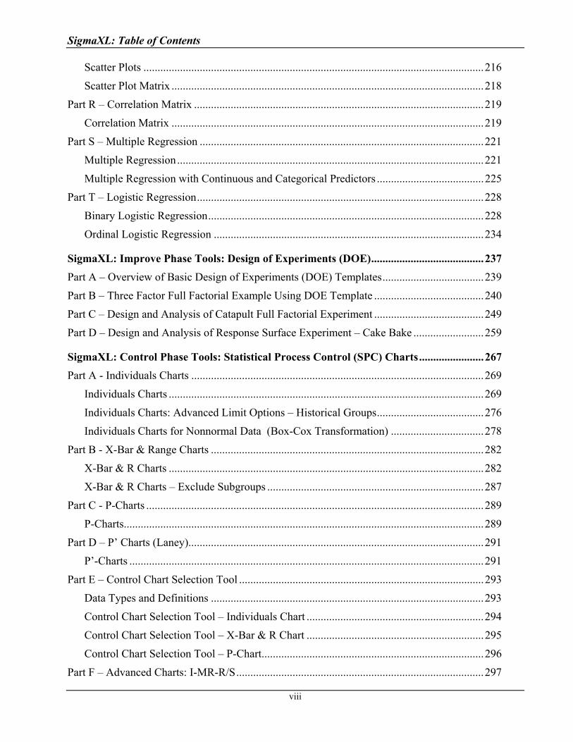
SigmaXL: Table of Contents
viii
Scatter Plots .........................................................................................................................216
Scatter Plot Matrix ...............................................................................................................218
Part R – Correlation Matrix .......................................................................................................219
Correlation Matrix ...............................................................................................................219
Part S – Multiple Regression .....................................................................................................221
Multiple Regression.............................................................................................................221
Multiple Regression with Continuous and Categorical Predictors ......................................225
Part T – Logistic Regression......................................................................................................228
Binary Logistic Regression..................................................................................................228
Ordinal Logistic Regression ................................................................................................234
SigmaXL: Improve Phase Tools: Design of Experiments (DOE)........................................237
Part A – Overview of Basic Design of Experiments (DOE) Templates....................................239
Part B – Three Factor Full Factorial Example Using DOE Template .......................................240
Part C – Design and Analysis of Catapult Full Factorial Experiment .......................................249
Part D – Design and Analysis of Response Surface Experiment – Cake Bake .........................259
SigmaXL: Control Phase Tools: Statistical Process Control (SPC) Charts.......................267
Part A - Individuals Charts ........................................................................................................269
Individuals Charts ................................................................................................................269
Individuals Charts: Advanced Limit Options – Historical Groups......................................276
Individuals Charts for Nonnormal Data (Box-Cox Transformation) .................................278
Part B - X-Bar & Range Charts .................................................................................................282
X-Bar & R Charts ................................................................................................................282
X-Bar & R Charts – Exclude Subgroups .............................................................................287
Part C - P-Charts ........................................................................................................................289
P-Charts................................................................................................................................289
Part D – P’ Charts (Laney).........................................................................................................291
P’-Charts ..............................................................................................................................291
Part E – Control Chart Selection Tool .......................................................................................293
Data Types and Definitions .................................................................................................293
Control Chart Selection Tool – Individuals Chart ...............................................................294
Control Chart Selection Tool – X-Bar & R Chart ...............................................................295
Control Chart Selection Tool – P-Chart...............................................................................296
Part F – Advanced Charts: I-MR-R/S........................................................................................297

SigmaXL: Table of Contents
ix
I-MR-R Charts .....................................................................................................................297
SigmaXL Appendix: Statistical Details for Nonnormal Distributions and Transformations301
Statistical Details for Nonnormal Distributions and Transformations ......................................303
Maximum Likelihood Estimation (MLE)............................................................................303
Distributions .......................................................................................................................304
Transformations.................................................................................................................314
Automatic Best Fit ............................................................................................................317
Process Capability Indices (Nonnormal) .......................................................................318
Control Charts (Nonnormal) ............................................................................................319

Copyright © 2004-2011, SigmaXL Inc.
SigmaXL® Feature List Summary, What’s New in Version 6.0 & 6.1,
Installation Notes, System Requirements and Getting Help


SigmaXL: What’s New, Installation Notes, Getting Help and Product Registration
13
SigmaXL Version 6.1 Feature List Summary
SigmaXL: What’s New, Installation Notes, Getting Help and Product Registration
14
SigmaXL: What’s New, Installation Notes, Getting Help and Product Registration
15
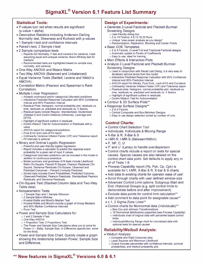
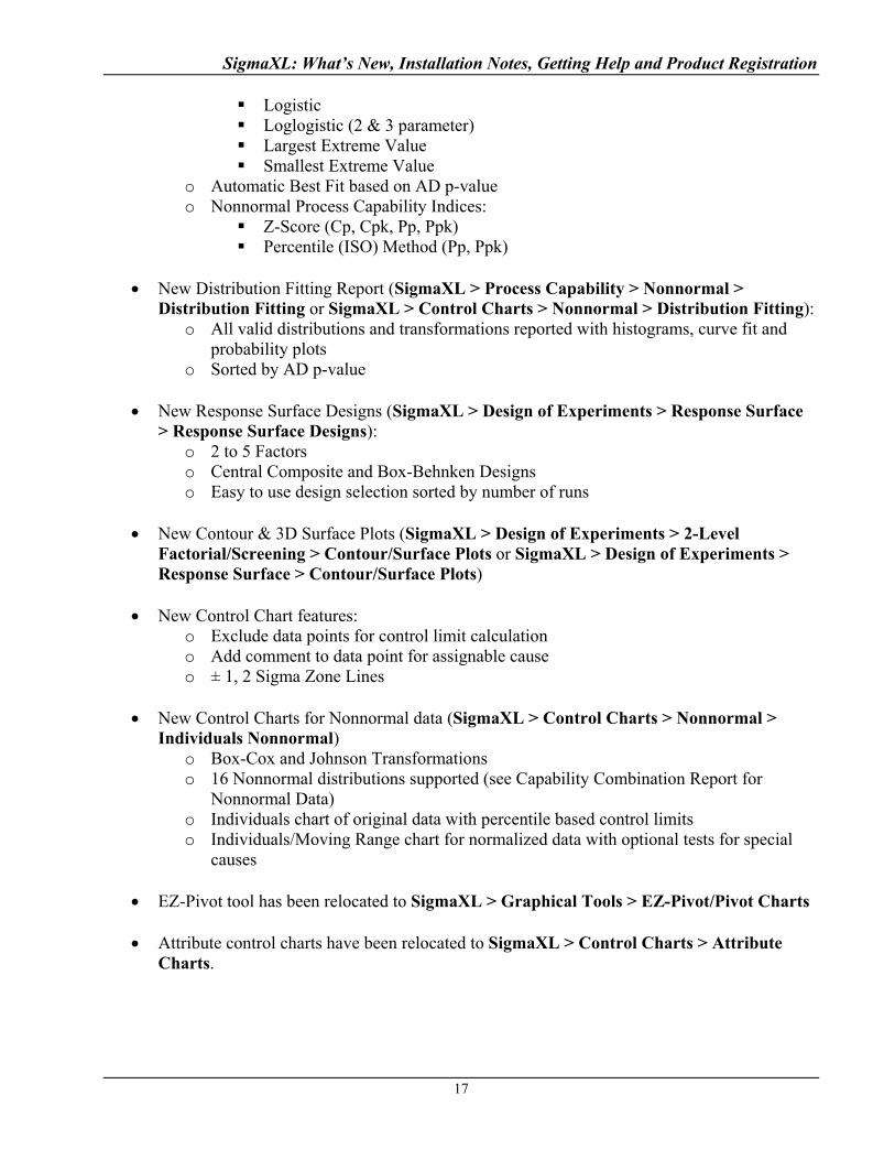
What’s New in Versions 6.0 & 6.1
New features in SigmaXL Version 6.1 include:
Now compatible with Excel 2010 64-bit version
Updated Cause & Effect (XY) Matrix Template with Pareto Chart option
Updated Failure Mode & Effects Analysis (FMEA) Template with Risk Priority Number (RPN) Sort
Updated Gage R&R Study (MSA) Template with Create Stacked Column Format for “Analyze Gage R&R” >> button
Updated Attribute MSA Template with Create Stacked Column Format to Analyze with “Attribute MSA (Binary)” >> button
Add Data menu options for Control Charts now include: “Add Data to this Control Chart” and “Add Data to all Control Charts”
Capability Combination Report, Distribution Fitting and Control Charts for nonnormal data have updated dialogs with the distribution selection options displayed visually. This makes it easier to determine which distribution to select.
New features in SigmaXL Version 6.0 include:
Powerful Excel Worksheet Manager (SigmaXL > Worksheet Manager) o List all open Excel workbooks o Display all worksheets and chart sheets in selected workbook o Quickly select worksheet or chart sheet of interest
Reorganized Templates and Calculators (SigmaXL > Templates and Calculators >):
o DMAIC & DFSS Templates o Lean Templates o Basic Graphical Templates o Basic Statistical Templates o Probability Distribution Calculators o Basic MSA Templates o Basic Process Capability Templates o Basic DOE Templates o Basic Control Chart Templates
Templates are also available within each menu section:

SigmaXL: What’s New, Installation Notes, Getting Help and Product Registration
16
o Basic Graphical Templates (SigmaXL > Graphical Tools > Basic Graphical Templates)
o Basic Statistical Templates (SigmaXL > Statistical Tools > Basic Statistical Templates)
o Basic MSA Templates (SigmaXL > Measurement Systems Analysis > Basic MSA Templates)
o Basic Process Capability Templates (SigmaXL > Process Capability > Basic Process Capability Templates)
o Basic DOE Templates (SigmaXL > Design of Experiments > Basic DOE Templates)
o Basic Control Chart Templates (SigmaXL > Control Charts > Basic Control Chart Templates)
New Lean Template (SigmaXL > Templates and Calculators > Lean):
o Value Stream Mapping
New Statistical Templates (SigmaXL > Templates and Calculators > Basic Statistical Templates or SigmaXL > Statistical Tools > Basic Statistical Templates):
o 1 Sample t Confidence Interval for Mean o 2 Sample t-Test (Assume Equal Variances) o 2 Sample t-Test (Assume Unequal Variances) o 2 Sample F-Test (Compare 2 StDevs) o 2 Proportions Test & Fisher’s Exact
New Probability Distribution Calculators (SigmaXL > Templates and Calculators >
Probability Distribution Calculators): o Normal, Lognormal, Exponential, Weibull o Binomial, Poisson, Hypergeometric
New Random Number Generators (SigmaXL > Data Manipulation > Random Data):
o Uniform (Continuous & Integer) o Lognormal o Weibull, Exponential o Triangular
New Capability Combination Report for Nonnormal Data ( SigmaXL > Process Capability
> Nonnormal > Capability Combination Report (Individuals Nonnormal) ): o Box-Cox Transformation (includes an automatic threshold option so that data with
negative values can be transformed) o Johnson Transformation o Distributions supported:
Half-Normal Lognormal (2 & 3 parameter) Exponential (1 & 2 parameter) Weibull (2 & 3 parameter) Beta (2 & 4 parameter) Gamma (2 & 3 parameter)
SigmaXL: What’s New, Installation Notes, Getting Help and Product Registration
17
Logistic Loglogistic (2 & 3 parameter) Largest Extreme Value Smallest Extreme Value
o Automatic Best Fit based on AD p-value o Nonnormal Process Capability Indices:
Z-Score (Cp, Cpk, Pp, Ppk) Percentile (ISO) Method (Pp, Ppk)
New Distribution Fitting Report (SigmaXL > Process Capability > Nonnormal >
Distribution Fitting or SigmaXL > Control Charts > Nonnormal > Distribution Fitting): o All valid distributions and transformations reported with histograms, curve fit and
probability plots o Sorted by AD p-value
New Response Surface Designs (SigmaXL > Design of Experiments > Response Surface
> Response Surface Designs): o 2 to 5 Factors o Central Composite and Box-Behnken Designs o Easy to use design selection sorted by number of runs
New Contour & 3D Surface Plots (SigmaXL > Design of Experiments > 2-Level
Factorial/Screening > Contour/Surface Plots or SigmaXL > Design of Experiments > Response Surface > Contour/Surface Plots)
New Control Chart features:
o Exclude data points for control limit calculation o Add comment to data point for assignable cause o ± 1, 2 Sigma Zone Lines
New Control Charts for Nonnormal data (SigmaXL > Control Charts > Nonnormal >
Individuals Nonnormal) o Box-Cox and Johnson Transformations o 16 Nonnormal distributions supported (see Capability Combination Report for
Nonnormal Data) o Individuals chart of original data with percentile based control limits o Individuals/Moving Range chart for normalized data with optional tests for special
causes
EZ-Pivot tool has been relocated to SigmaXL > Graphical Tools > EZ-Pivot/Pivot Charts
Attribute control charts have been relocated to SigmaXL > Control Charts > Attribute Charts.
SigmaXL: What’s New, Installation Notes, Getting Help and Product Registration
Installation Notes
1. This installation procedure requires that you have administrator rights to install software on your computer. Also please ensure that you have the latest Microsoft Office service pack by using Windows Update before installing SigmaXL.
2. You will be required to activate SigmaXL. To do so, you should ensure that you are connected to the Internet. If you do not have Internet access or have firewall restrictions, you can activate using telephone or e-mail. Note that activation is required within 30 days of first use. For more information on product activation, see http://www.sigmaxl.com/Activating_SigmaXL.htm or www.SigmaXL.com, click Help & Support > Product Activation FAQ Section.
3. Please uninstall any earlier (or trial) versions of SigmaXL.
4. If you are installing from a CD, the SigmaXL installer will run automatically. If you
downloaded SigmaXL, please double-click on the file SigmaXL_Setup.msi .
5. We recommend that you accept all defaults during the install. Enter your User Name and Company Name. Setup type should be Complete. The installer will create a desktop shortcut to SigmaXL.
6. To start SigmaXL double-click on the SigmaXL desktop icon or click Start > Programs > SigmaXL > V6 > SigmaXL. Tip: SigmaXL can also be automatically started when you start Excel. After starting SigmaXL, you can enable automatic start by clicking SigmaXL > Help > Automatically Load SigmaXL. If you need to disable this feature, click Excel Tools > Add-Ins and uncheck SigmaXL, click OK (to disable in Excel 2007: Office Button | Excel Options | Add-Ins, select Manage: Excel Add-ins, click Go… uncheck SigmaXL, click OK;Excel 2010 : File | Options… ). This feature should be used with caution in cases where you automatically start other third-party Excel add-ins. The Excel menu may become cluttered and potential software conflicts may occur.
18
SigmaXL: What’s New, Installation Notes, Getting Help and Product Registration
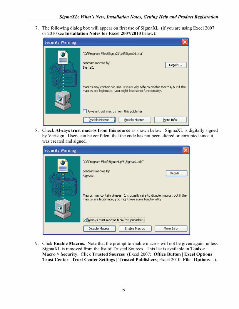
7. The following dialog box will appear on first use of SigmaXL (if you are using Excel 2007 or 2010 see Installation Notes for Excel 2007/2010 below):
8. Check Always trust macros from this source as shown below. SigmaXL is digitally signed by Verisign. Users can be confident that the code has not been altered or corrupted since it was created and signed.
9. Click Enable Macros. Note that the prompt to enable macros will not be given again, unless SigmaXL is removed from the list of Trusted Sources. This list is available in Tools > Macro > Security. Click Trusted Sources (Excel 2007: Office Button | Excel Options | Trust Center | Trust Center Settings | Trusted Publishers; Excel 2010: File | Options…).
19
SigmaXL: What’s New, Installation Notes, Getting Help and Product Registration
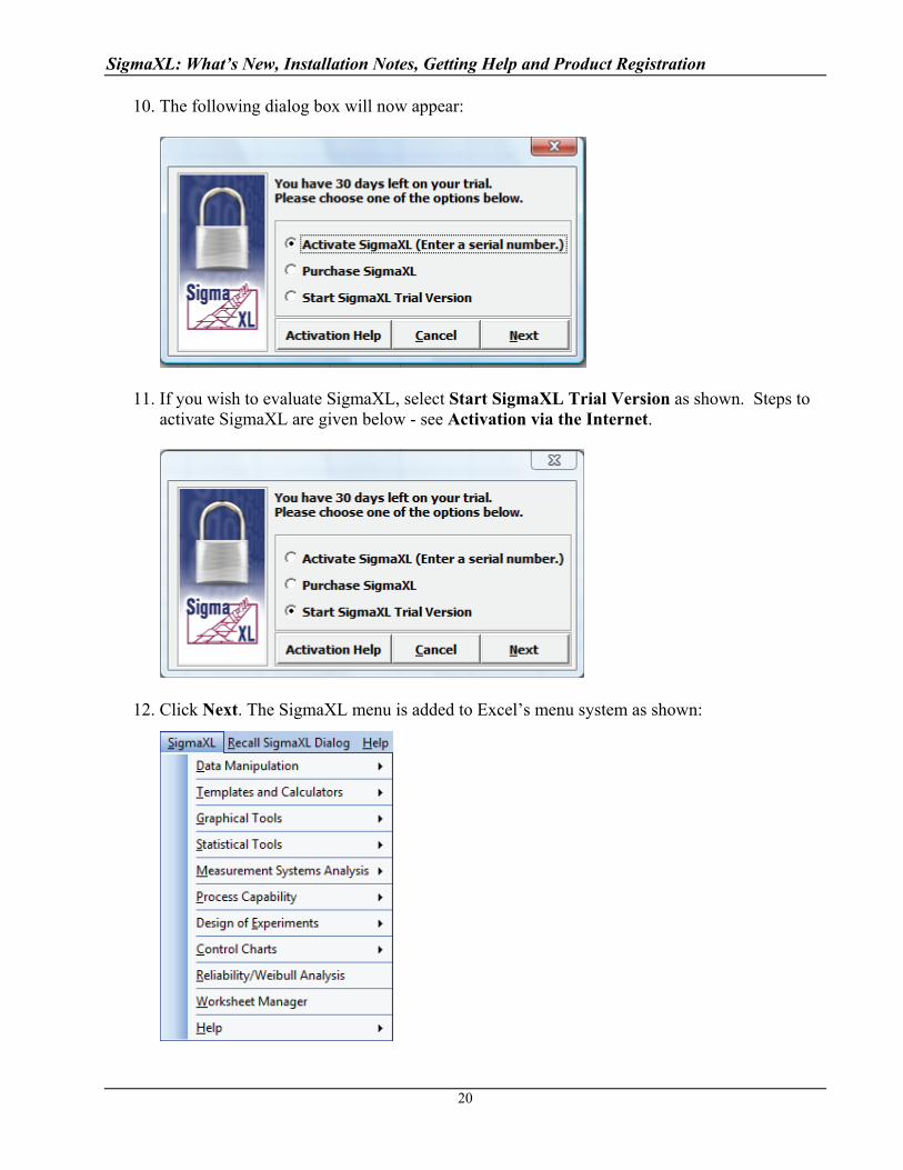
10. The following dialog box will now appear:
11. If you wish to evaluate SigmaXL, select Start SigmaXL Trial Version as shown. Steps to activate SigmaXL are given below - see Activation via the Internet.
12. Click Next. The SigmaXL menu is added to Excel’s menu system as shown:
20

SigmaXL: What’s New, Installation Notes, Getting Help and Product Registration
13. In Excel 2007/2010, the SigmaXL Ribbon appears as shown:
Activation via the Internet:
Please proceed with the following steps if you have a valid serial number and your computer is connected to the Internet. If you do not have an Internet connection, activation can be completed by e-mail or telephone (see steps below). If you purchased SigmaXL as a download, you received the serial number by e-mail. If you purchased a CD, the serial number is on the label of the CD. If your trial has timed out and you do not have a serial number but wish to purchase a SigmaXL license, please click Purchase SigmaXL in the Activation Wizard Box and this will take you to SigmaXL’s order page http://www.sigmaxl.com/Order%20SigmaXL.htm. You can also call 1-888-SigmaXL (1-888-744-6295) or 1-416-236-5877 to place an order. 1. In the Activation Wizard box select Activate SigmaXL (Enter a serial number).
2. Click Next. Enter your serial number as shown below. If you received the serial number by e-mail, simply copy and paste from the e-mail. Note that the serial number GGGGG-RRRRR-TTTTT-GGGGG-RRRRR-TTTTT-0 is given as an example – it will not activate your copy of SigmaXL.
21
SigmaXL: What’s New, Installation Notes, Getting Help and Product Registration
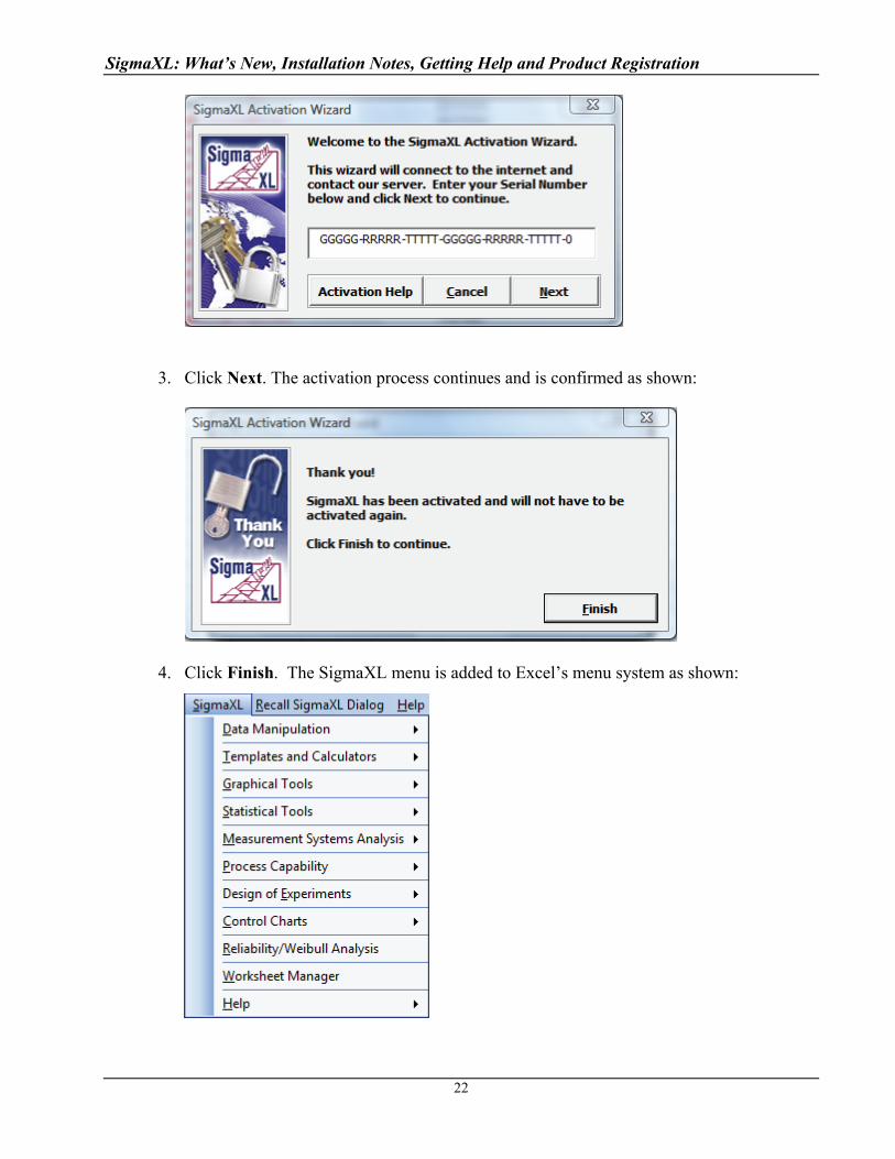
3. Click Next. The activation process continues and is confirmed as shown:
4. Click Finish. The SigmaXL menu is added to Excel’s menu system as shown:
22
SigmaXL: What’s New, Installation Notes, Getting Help and Product Registration
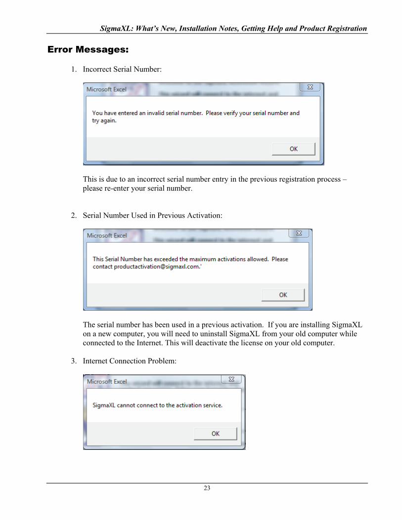
Error Messages: 1. Incorrect Serial Number:
This is due to an incorrect serial number entry in the previous registration process – please re-enter your serial number.
2. Serial Number Used in Previous Activation:
The serial number has been used in a previous activation. If you are installing SigmaXL on a new computer, you will need to uninstall SigmaXL from your old computer while connected to the Internet. This will deactivate the license on your old computer.
3. Internet Connection Problem:
23
SigmaXL: What’s New, Installation Notes, Getting Help and Product Registration
If you do not have an Internet connection, please activate by e-mail or telephone.
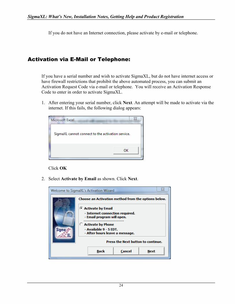
Activation via E-Mail or Telephone: If you have a serial number and wish to activate SigmaXL, but do not have internet access or have firewall restrictions that prohibit the above automated process, you can submit an Activation Request Code via e-mail or telephone. You will receive an Activation Response Code to enter in order to activate SigmaXL. 1. After entering your serial number, click Next. An attempt will be made to activate via the
internet. If this fails, the following dialog appears:
Click OK
2. Select Activate by Email as shown. Click Next.
24

SigmaXL: What’s New, Installation Notes, Getting Help and Product Registration
3. An email is created containing your serial number and request code. This email is automatically sent to [email protected] using your email program. You will receive a reply e-mail with the Activation Response Code. Copy and paste the Activation Response Code into the dialog box shown below and click Finish to activate.
4. To activate by phone, select Activate by Phone as shown:
5. Click Next.
25

SigmaXL: What’s New, Installation Notes, Getting Help and Product Registration
6. Call SigmaXL at 1-888-SigmaXL (1-888-744-6295) or 1-416-236-5877 to provide your Activation Request Code. You will verbally receive the Activation Response Code which is then entered into the above dialog box. Click Finish to activate.
26
SigmaXL: What’s New, Installation Notes, Getting Help and Product Registration
Installation Notes for Excel 2007/2010
1. The previous installation notes apply to Excel 2007/2010 as well, but there are differences in the security warning and menu access.
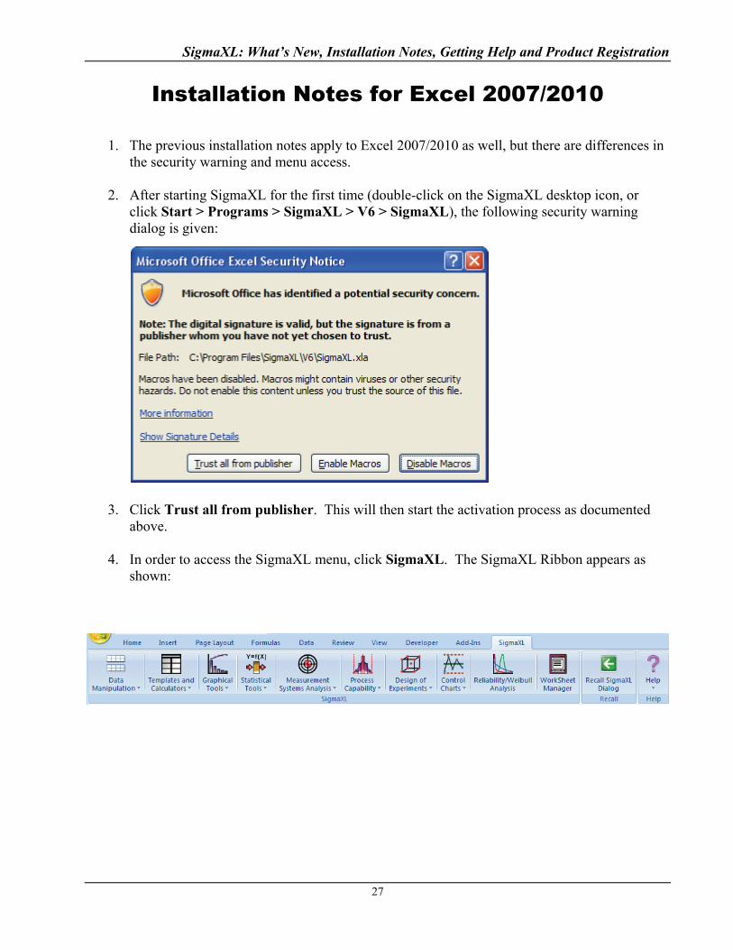
2. After starting SigmaXL for the first time (double-click on the SigmaXL desktop icon, or click Start > Programs > SigmaXL > V6 > SigmaXL), the following security warning dialog is given:
3. Click Trust all from publisher. This will then start the activation process as documented above.
4. In order to access the SigmaXL menu, click SigmaXL. The SigmaXL Ribbon appears as shown:
27
SigmaXL: What’s New, Installation Notes, Getting Help and Product Registration
5. If SigmaXL’s Ribbon is not available: You may need to specify SigmaXL’s folder as a trusted location (these steps are not necessary if you see the SigmaXL Ribbon):
Click the Office Button: (Excel 2010: File)
Select Excel Options: (Excel 2010: Options)
Select Trust Center:
Click Trust Center Settings:
Select Trusted Locations:
Click Add New Location:
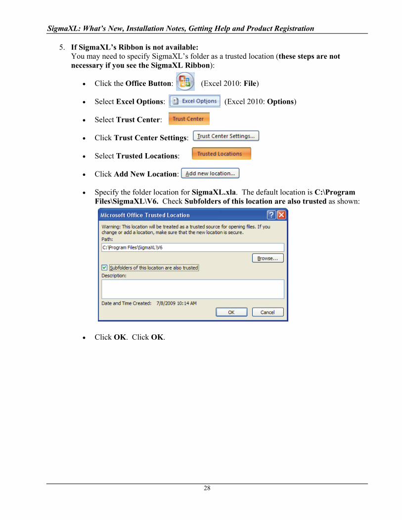
Specify the folder location for SigmaXL.xla. The default location is C:\Program Files\SigmaXL\V6. Check Subfolders of this location are also trusted as shown:
Click OK. Click OK.
28
SigmaXL: What’s New, Installation Notes, Getting Help and Product Registration
SigmaXL® Defaults and Menu Options
Clear Saved Defaults
Clear Saved Defaults will reset all saved defaults such as Pareto and Multi-Vari Chart settings,
saved control limits, and dialog box settings. All settings are restored to the original installation
defaults.
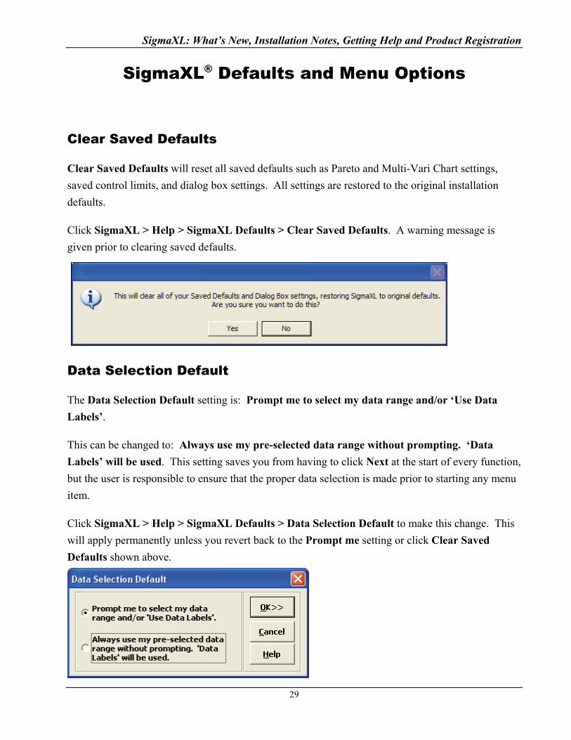
Click SigmaXL > Help > SigmaXL Defaults > Clear Saved Defaults. A warning message is
given prior to clearing saved defaults.
Data Selection Default
The Data Selection Default setting is: Prompt me to select my data range and/or ‘Use Data
Labels’.
This can be changed to: Always use my pre-selected data range without prompting. ‘Data
Labels’ will be used. This setting saves you from having to click Next at the start of every function,
but the user is responsible to ensure that the proper data selection is made prior to starting any menu
item.
Click SigmaXL > Help > SigmaXL Defaults > Data Selection Default to make this change. This
will apply permanently unless you revert back to the Prompt me setting or click Clear Saved
Defaults shown above.
29

SigmaXL: What’s New, Installation Notes, Getting Help and Product Registration
Menu Options (Classical or DMAIC)
The default SigmaXL menu system groups tools by category, but this can be changed to the Six
Sigma DMAIC format.
Click SigmaXL > Help > SigmaXL Defaults > Menu Options – Set SigmaXL’s Menu to
Classical or DMAIC. The Set Menu dialog allows you to choose between Classical (default) and
DMAIC:
If you select the DMAIC format, the SigmaXL menu layout will be as shown:
In Excel 2007/2010, the DMAIC Menu Ribbon appears as shown:
All SigmaXL tools are available with this menu format, but they are categorized using the Six Sigma
DMAIC phase format. Note that some tools will appear in more than one phase.
This workbook uses the classical (default) menu format, but the chapters are organized as Measure,
Analyze, Improve and Control.
30
SigmaXL: What’s New, Installation Notes, Getting Help and Product Registration
31
SigmaXL® System Requirements
Minimum System Requirements:
Computer and processor: 500 megahertz (MHz) processor or higher.
Memory: 512 megabytes (MB) of RAM or greater.
Hard disk: 70 MB of available hard-disk space.
Drive: CD-ROM or DVD drive.
Display: 1024x768 or higher resolution monitor.
Operating system: Microsoft Windows XP with Service Pack (SP) 2, or later operating system.
Microsoft Excel version: Excel XP, Excel 2003, Excel 2007, or Excel 2010 with latest service
packs installed.
SigmaXL: What’s New, Installation Notes, Getting Help and Product Registration
32
Getting Help and Product Registration
To access the help system, please click SigmaXL > Help > Help. Technical support is available by phone at 1-866-475-2124 (toll-free in North America) or 1-416-236-5877 or e-mail [email protected]. Please note that registered users obtain free technical support and upgrades for one year from date of purchase. Optional maintenance is available for purchase prior to the anniversary date. To register by web, simply click SigmaXL > Help > Register SigmaXL.

Copyright © 2004-2011, SigmaXL Inc.
Introduction to SigmaXL® Data Format and Tools Summary

SigmaXL: Introduction to Data Format and Tools Summary
35
Introduction
SigmaXL is a powerful but easy to use Excel Add-In that will enable you to Measure, Analyze, Improve and Control your service, transactional, and manufacturing processes. This is the ideal cost effective tool for Six Sigma Green Belts and Black Belts, Quality and Business Professionals, Engineers, and Managers. SigmaXL will help you in your problem solving and process improvement efforts by enabling you to easily slice and dice your data, quickly separating the “vital few” factors from the “trivial many”. This tool will also help you to identify and validate root causes and sources of variation, which then helps to ensure that you develop permanent corrective actions and/or improvements.
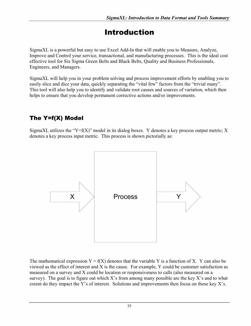
The Y=f(X) Model SigmaXL utilizes the “Y=f(X)” model in its dialog boxes. Y denotes a key process output metric; X denotes a key process input metric. This process is shown pictorially as: The mathematical expression Y = f(X) denotes that the variable Y is a function of X. Y can also be viewed as the effect of interest and X is the cause. For example, Y could be customer satisfaction as measured on a survey and X could be location or responsiveness to calls (also measured on a survey). The goal is to figure out which X’s from among many possible are the key X’s and to what extent do they impact the Y’s of interest. Solutions and improvements then focus on those key X’s.
ProcessX Y
SigmaXL: Introduction to Data Format and Tools Summary
36
Data Types: Continuous Versus Discrete X and Y metrics can each be continuous or discrete. A continuous measure will have readings on a continuous scale where a mid-point has meaning. For example, in a customer satisfaction survey using a 1 to 5 score, the value 3.5 has meaning. Other examples of continuous measures include cycle time, thickness, and weight. A discrete measure is categorical in nature. If we have Customer Types 1, 2, and 3, customer type 1.5 has no meaning. Other examples of discrete measures include defect counts and number of customer complaints. It is possible to have various combinations of discrete/continuous X’s and discrete/continuous Y’s. Some examples are given below: Examples of Discrete (Category) X and Discrete Y
X = Customer Type, Y = Number of Complaints
X = Product Type, Y = Number of Defects
X = Day Shift vs. Night Shift, Y = Proportion of Defective Units Examples of Discrete (Category) X and Continuous Y
X = Customer Type, Y = Customer Satisfaction (1-5)
X = Before Improvement vs. After Improvement, Y = Customer Satisfaction (1-5)
X = Location, Y = Order to Delivery Time Examples of Continuous X and Discrete Y
X = Responsiveness to Calls (1-5), Y = Number of Complaints X = Process Temperature, Y = Number of Defects
Examples of Continuous X and Continuous Y
X = Responsiveness to Calls (1-5), Y = Customer Satisfaction (1-5) X = Amount of Loan ($), Y = Cycle Time (Loan Application to Approval)
Note that in SigmaXL, a discrete X can be text or numeric, but a continuous X must be numeric. Y’s must be numeric. If Y is discrete, count data will be required. If the data of interest is discrete text, it should be referenced as X1 and SigmaXL will automatically search through the text data to obtain a count (applicable for Pareto, Chi-Square and EZ-Pivot tools).
SigmaXL: Introduction to Data Format and Tools Summary
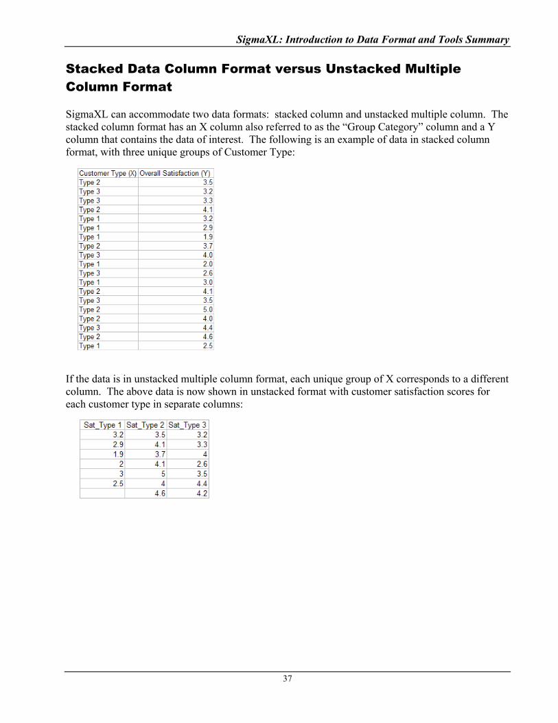
Stacked Data Column Format versus Unstacked Multiple Column Format SigmaXL can accommodate two data formats: stacked column and unstacked multiple column. The stacked column format has an X column also referred to as the “Group Category” column and a Y column that contains the data of interest. The following is an example of data in stacked column format, with three unique groups of Customer Type: If the data is in unstacked multiple column format, each unique group of X corresponds to a different column. The above data is now shown in unstacked format with customer satisfaction scores for each customer type in separate columns:
37
SigmaXL: Introduction to Data Format and Tools Summary
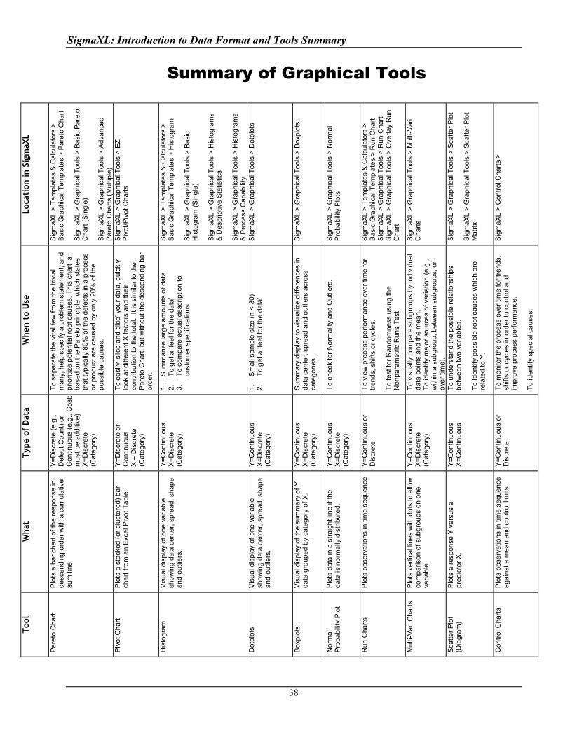
Summary of Graphical Tools
38
Tool
W
hat
Type
of
Dat
a W
hen
to U
se
Loca
tion
in S
igm
aXL
Pa
reto
Cha
rt
Plo
ts a
ba
r ch
art
of t
he
resp
ons
e in
de
scen
ding
ord
er
with
a c
um
ulat
ive
su
m li
ne.
Y=
Dis
cre
te (
e.g
.,
De
fect
Cou
nt)
or
Co
ntin
uous
(e.
g.,
Cos
t; m
ust b
e a
dditi
ve)
X=
Dis
cre
te
(Ca
teg
ory)
To
se
pa
rate
the
vita
l fe
w fr
om
the
triv
ial
man
y, h
elp
spe
cify
a p
robl
em s
tate
men
t, a
nd
pri
ori
tize
pot
en
tial r
oot c
aus
es. T
his
cha
rt is
ba
sed
on
the
Pa
reto
prin
cip
le, w
hic
h st
ate
s th
at t
ypic
ally
80
% o
f th
e d
efe
cts
in a
pro
cess
or
pro
duct
are
ca
use
d b
y on
ly 2
0% o
f th
e po
ssib
le c
aus
es.
Sig
ma
XL
> T
em
plat
es
& C
alcu
lato
rs >
B
asi
c G
raph
ical
Te
mpl
ates
> P
are
to C
hart
S
igm
aX
L >
Gra
phic
al T
ool
s >
Bas
ic P
aret
o
Ch
art
(Sin
gle)
S
igm
aX
L >
Gra
phic
al T
ool
s >
Adv
ance
d P
are
to C
hart
s (M
ulti
ple
) P
ivot
Ch
art
Plo
ts a
sta
cked
(o
r cl
uste
red
) b
ar
cha
rt fr
om
an
Exc
el P
ivo
t Tab
le.
Y=
Dis
cre
te o
r C
ont
inuo
us
X =
Dis
cret
e (C
ate
gor
y)
To
eas
ily ‘s
lice
an
d di
ce’ y
our
data
, qu
ickl
y lo
ok
at d
iffe
rent
X f
acto
rs a
nd
the
ir co
ntr
ibu
tion
to th
e to
tal.
It i
s si
mila
r to
the
P
are
to C
hart
, but
with
out
the
des
cend
ing
bar
orde
r.
Sig
ma
XL
> G
raph
ica
l To
ols
> E
Z-
Piv
ot/P
ivo
t C
ha
rts
His
tog
ram
V
isu
al d
ispl
ay
of o
ne v
aria
ble
sho
win
g da
ta c
ente
r, s
pre
ad,
sha
pe
and
outli
ers.
Y=
Con
tinu
ous
X=
Dis
cre
te
(Ca
teg
ory)
1.
Sum
ma
rize
larg
e a
mou
nts
of d
ata
2.
T
o g
et
a ‘f
eel f
or th
e da
ta’
3.
To
com
pare
act
ual d
escr
iptio
n to
cu
sto
me
r sp
ecifi
catio
ns
Sig
ma
XL
> T
em
plat
es
& C
alcu
lato
rs >
B
asi
c G
raph
ical
Te
mpl
ates
> H
isto
gra
m
Sig
ma
XL
> G
raph
ica
l To
ols
> B
asic
H
isto
gra
m (
Sin
gle
) S
igm
aX
L >
Gra
phic
al T
ool
s >
His
togr
ams
& D
escr
iptiv
e S
tatis
tics
Sig
ma
XL
> G
raph
ica
l To
ols
> H
isto
gram
s &
Pro
cess
Cap
abili
ty
Do
tplo
ts
Vis
ual
dis
pla
y of
one
var
iabl
e sh
ow
ing
data
cen
ter,
sp
read
, sh
ape
an
d ou
tlier
s.
Y=
Con
tinu
ous
X=
Dis
cre
te
(Ca
teg
ory)
1.
Sm
all s
ampl
e si
ze (
n <
30)
2.
T
o g
et
a ‘f
eel f
or th
e da
ta’
Sig
ma
XL
> G
raph
ica
l To
ols
> D
otp
lots
Bo
xplo
ts
Vis
ual
dis
pla
y of
the
sum
ma
ry o
f Y
da
ta g
rou
ped
by
cate
gor
y of
X.
Y=
Con
tinu
ous
X=
Dis
cre
te
(Ca
teg
ory)
Su
mm
ary
disp
lay
to v
isu
aliz
e di
ffer
ence
s in
da
ta c
ente
r, s
pre
ad a
nd o
utlie
rs a
cro
ss
cate
go
ries.
Sig
ma
XL
> G
raph
ica
l To
ols
> B
oxpl
ots
No
rma
l P
rob
abili
ty P
lot
Plo
ts d
ata
in a
str
aig
ht li
ne
if th
e
da
ta is
nor
ma
lly d
istr
ibut
ed
. Y
=C
ontin
uou
s X
=D
iscr
ete
(C
ate
gor
y)
To
ch
eck
for
No
rmal
ity a
nd O
utlie
rs.
Sig
ma
XL
> G
raph
ica
l To
ols
> N
orm
al
Pro
bab
ility
Plo
ts
Ru
n C
har
ts
Plo
ts o
bse
rva
tion
s in
tim
e se
que
nce
Y
=C
ontin
uou
s or
D
iscr
ete
To
vie
w p
roce
ss p
erfo
rman
ce o
ver
time
fo
r tr
ends
, sh
ifts
or
cycl
es.
To
test
fo
r R
an
dom
ness
usi
ng
the
N
onp
aram
etric
Run
s T
est
Sig
ma
XL
> T
em
plat
es
& C
alcu
lato
rs >
B
asi
c G
raph
ical
Te
mpl
ates
> R
un C
har
t S
igm
aX
L >
Gra
phic
al T
ool
s >
Ru
n C
har
t S
igm
aX
L >
Gra
phic
al T
ool
s >
Ove
rlay
Ru
n C
har
t
Mul
ti-V
ari
Ch
art
s P
lots
ve
rtic
al li
nes
with
do
ts to
allo
w
com
paris
on
of s
ubgr
oups
on
on
e va
riab
le.
Y=
Con
tinu
ous
X=
Dis
cre
te
(Ca
teg
ory)
To
vis
ually
co
mpa
re s
ubg
roup
s by
ind
ivid
ual
data
poi
nts
and
the
me
an.
T
o id
ent
ify m
ajo
r so
urce
s o
f var
iatio
n (e
.g.,
with
in a
sub
grou
p, b
etw
een
subg
roup
s, o
r o
ver
time)
.
Sig
ma
XL
> G
raph
ica
l To
ols
> M
ulti-
Var
i C
har
ts
Sca
tte
r P
lot
(Dia
gra
m)
Plo
ts a
res
pon
se Y
ve
rsus
a
pred
icto
r X
. Y
=C
ontin
uou
s X
=C
ontin
uou
s T
o u
nder
stan
d th
e p
ossi
ble
re
latio
nshi
ps
betw
een
tw
o va
riabl
es.
To
ide
ntif
y po
ssib
le r
oot c
aus
es w
hic
h a
re
rela
ted
to Y
.
Sig
ma
XL
> G
raph
ica
l To
ols
> S
catt
er P
lot
Sig
ma
XL
> G
raph
ica
l To
ols
> S
catt
er P
lot
Mat
rix
Co
ntro
l Cha
rts
Plo
ts o
bse
rva
tion
s in
tim
e se
que
nce
ag
ains
t a m
ean
and
con
tro
l lim
its.
Y=
Con
tinu
ous
or
Dis
cret
e T
o m
onito
r th
e p
roce
ss o
ver
time
for
tre
nds,
sh
ifts
or c
ycle
s in
ord
er to
con
tro
l and
im
pro
ve p
roce
ss p
erfo
rma
nce
. T
o id
en
tify
spec
ial c
au
ses.
Sig
ma
XL
> C
ontr
ol C
hart
s >
SigmaXL: Introduction to Data Format and Tools Summary
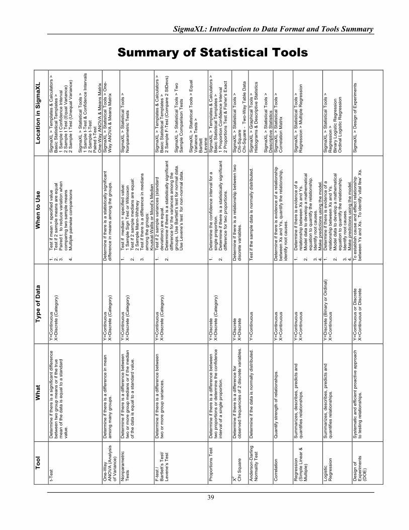
Summary of Statistical Tools
39
To
ol
Wh
at
Typ
e o
f D
ata
W
he
n t
o U
se
L
oc
ati
on
in
Sig
ma
XL
t-T
est
D
ete
rmin
e if
th
ere
is a
sig
nifi
can
t d
iffe
ren
ce
be
twe
en
tw
o g
rou
p m
ea
ns
or
if th
e t
rue
m
ea
n o
f th
e d
ata
is e
qu
al t
o a
sta
nd
ard
va
lue
.
Y=
Co
ntin
uo
us
X=
Dis
cre
te (
Ca
teg
ory
) 1
. T
est
if m
ea
n =
sp
eci
fied
va
lue
2
. T
est
if 2
sa
mp
le m
ea
ns
are
eq
ua
l 3
. P
air
ed
t: t
o r
ed
uce
va
ria
tion
wh
en
co
mp
ari
ng
tw
o s
am
ple
me
an
s 4
. M
ulti
ple
pa
irw
ise
co
mp
ari
son
s
Sig
ma
XL
> T
em
pla
tes
& C
alc
ula
tors
>
Ba
sic
Sta
tistic
al T
em
pla
tes
>
1 S
am
ple
t C
on
fide
nce
In
terv
al
2 S
am
ple
t T
est
(E
qu
al V
ari
an
ce)
2 S
am
ple
t T
est
(U
ne
qu
al V
ari
an
ce)
Sig
ma
XL
> S
tatis
tica
l To
ols
>
1 S
am
ple
t-T
est
& C
on
fide
nce
In
terv
als
2
Sa
mp
le t
-Te
st
Pa
ire
d t
-Te
st
On
e-W
ay
AN
OV
A &
Me
an
s M
atr
ix
On
e-W
ay
AN
OV
A (
An
aly
sis
of V
ari
an
ce)
De
term
ine
if th
ere
is a
diff
ere
nce
in m
ea
n
am
on
g m
an
y g
rou
ps.
Y
=C
on
tinu
ou
s X
=D
iscr
ete
(C
ate
go
ry)
De
term
ine
if th
ere
is a
sta
tistic
ally
sig
nifi
can
t d
iffe
ren
ce in
me
an
s a
mo
ng
th
e g
rou
ps.
S
igm
aX
L >
Sta
tistic
al T
oo
ls >
On
e-
Wa
y A
NO
VA
& M
ea
ns
Ma
trix
No
np
ara
me
tric
T
est
s D
ete
rmin
e if
th
ere
is a
diff
ere
nce
be
twe
en
tw
o o
r m
ore
gro
up m
edia
ns
or
if th
e m
ed
ian
o
f th
e d
ata
is e
qu
al t
o a
sta
nd
ard
va
lue
.
Y=
Co
ntin
uo
us
X=
Dis
cre
te (
Ca
teg
ory
) 1
. T
est
if
me
dia
n =
sp
eci
fied
va
lue
:
1 S
am
ple
Sig
n T
est
or
Wilc
oxo
n
2.
Te
st if
2 s
am
ple
me
dia
ns
are
eq
ua
l:
2 S
am
ple
Ma
nn
-Wh
itne
y 3
. T
est
if th
ere
is a
diff
ere
nce
in m
ed
ian
s a
mo
ng
th
e g
rou
ps:
K
rusk
al-
Wa
llis
or
Mo
od
’s M
ed
ian
Sig
ma
XL
> S
tatis
tica
l To
ols
>
No
np
ara
me
tric
Te
sts
F-t
est
/
Ba
rtle
tt’s
Te
st/
Le
ven
e’s
Te
st
De
term
ine
if th
ere
is a
diff
ere
nce
be
twe
en
tw
o o
r m
ore
gro
up
va
ria
nce
s.
Y=
Co
ntin
uo
us
X=
Dis
cre
te (
Ca
teg
ory
) 1
. T
est
if 2
sa
mp
le v
ari
an
ces
(sta
nd
ard
d
evi
atio
ns)
are
eq
ua
l. 2
. D
ete
rmin
e if
th
ere
is a
sta
tistic
ally
sig
nifi
can
t d
iffe
ren
ce f
or
the
va
ria
nce
s a
mo
ng
th
e
gro
up
s. U
se B
art
lett
’s te
st fo
r n
orm
al d
ata
. U
se L
eve
ne
’s te
st
for
no
n-n
orm
al d
ata
.
Sig
ma
XL
> T
em
pla
tes
& C
alc
ula
tors
>
Ba
sic
Sta
tistic
al T
em
pla
tes
>
2 S
am
ple
F-T
est
(C
om
pa
re 2
StD
evs
) S
igm
aX
L >
Sta
tistic
al T
oo
ls >
Tw
o
Sa
mp
le C
om
pa
riso
n T
est
s S
igm
aX
L >
Sta
tistic
al T
oo
ls >
Eq
ua
l V
ari
an
ce T
est
s >
B
art
lett
L
eve
ne
P
rop
ort
ion
s T
est
D
ete
rmin
e if
th
ere
is a
diff
ere
nce
be
twe
en
tw
o p
rop
ort
ion
s o
r d
ete
rmin
e t
he
co
nfid
en
ce
inte
rva
l of a
sin
gle
pro
po
rtio
n.
Y=
Dis
cre
te
X=
Dis
cre
te (
Ca
teg
ory
) 1
. D
ete
rmin
e t
he
co
nfid
en
ce in
terv
al f
or
a
sin
gle
pro
po
rtio
n.
2.
De
term
ine
if t
he
re is
a s
tatis
tica
lly s
ign
ifica
nt
diff
ere
nce
fo
r tw
o p
rop
ort
ion
s.
Sig
ma
XL
> T
em
pla
tes
& C
alc
ula
tors
>
Ba
sic
Sta
tistic
al T
em
pla
tes
>
1 P
rop
ort
ion
Co
nfid
en
ce In
terv
al
2 P
rop
ort
ion
s T
est
& F
ish
er’
s E
xact
Χ2
Ch
i Sq
ua
re
De
term
ine
if th
ere
is a
diff
ere
nce
fo
r o
bse
rve
d f
req
ue
nci
es
of
2 d
iscr
ete
va
ria
ble
s.
Y=
Dis
cre
te
X=
Dis
cre
te
De
term
ine
if th
ere
is a
re
latio
nsh
ip b
etw
ee
n t
wo
d
iscr
ete
va
ria
ble
s.
Sig
ma
XL
> S
tatis
tica
l To
ols
>
Ch
i-S
qu
are
C
hi-
Sq
ua
re -
T
wo
-Wa
y T
ab
le D
ata
An
de
rso
n-D
arl
ing
N
orm
alit
y T
est
D
ete
rmin
e if
th
e d
ata
is n
orm
ally
dis
trib
ute
d.
Y=
Co
ntin
uo
us
Te
st if
th
e s
am
ple
da
ta is
no
rma
lly d
istr
ibu
ted
. S
igm
aX
L >
Gra
ph
ica
l To
ols
>
His
tog
ram
s &
De
scri
ptiv
e S
tatis
tics
Sig
ma
XL
> S
tatis
tica
l To
ols
>
De
scri
ptiv
e S
tatis
tics
Co
rre
latio
n
Qu
an
tify
stre
ng
th o
f re
latio
nsh
ips.
Y
=C
on
tinu
ou
s X
=C
on
tinu
ou
s D
ete
rmin
e if
th
ere
is e
vid
en
ce o
f a
re
latio
nsh
ip
be
twe
en
Xs
an
d Y
s, q
ua
ntif
y th
e r
ela
tion
ship
, id
en
tify
roo
t ca
use
s.
Sig
ma
XL
> S
tatis
tica
l To
ols
>
Co
rre
latio
n M
atr
ix
Re
gre
ssio
n
(Sim
ple
Lin
ea
r &
M
ulti
ple
)
Su
mm
ari
zes,
de
scri
be
s, p
red
icts
an
d
qu
an
tifie
s re
latio
nsh
ips.
Y
=C
on
tinu
ou
s X
=C
on
tinu
ou
s 1
. D
ete
rmin
e if
th
ere
is e
vid
en
ce o
f a
re
latio
nsh
ip b
etw
ee
n X
s a
nd
Ys.
2
. M
od
el d
ata
to
de
velo
p a
ma
the
ma
tica
l e
qu
atio
n to
qu
an
tify
the
re
latio
nsh
ip.
3.
Ide
ntif
y ro
ot ca
use
s.
4.
Ma
ke p
red
ictio
ns
usi
ng
th
e m
od
el.
Sig
ma
XL
> S
tatis
tica
l To
ols
>
Re
gre
ssio
n >
Mu
ltip
le R
eg
ress
ion
Lo
gis
tic
Re
gre
ssio
n
Su
mm
ari
zes,
de
scri
be
s, p
red
icts
an
d
qu
an
tifie
s re
latio
nsh
ips.
Y
=D
iscr
ete
(B
ina
ry o
r O
rdin
al)
X
=C
on
tinu
ou
s 1
. D
ete
rmin
e if
th
ere
is e
vid
en
ce o
f a
re
latio
nsh
ip b
etw
ee
n X
s a
nd
Ys.
2
. M
od
el d
ata
to
de
velo
p a
ma
the
ma
tica
l e
qu
atio
n to
qu
an
tify
the
re
latio
nsh
ip.
3.
Ide
ntif
y ro
ot ca
use
s.
4.
Ma
ke p
red
ictio
ns
usi
ng
th
e m
od
el.
Sig
ma
XL
> S
tatis
tica
l To
ols
>
Re
gre
ssio
n >
B
ina
ry L
og
istic
Re
gre
ssio
n
Ord
ina
l Lo
gis
tic R
eg
ress
ion
De
sig
n o
f E
xpe
rim
en
ts
(DO
E)
Sys
tem
atic
an
d e
ffic
ien
t p
roa
ctiv
e a
pp
roa
ch
to t
est
ing
re
latio
nsh
ips.
Y
=C
on
tinu
ou
s o
r D
iscr
ete
X
=C
on
tinu
ou
s o
r D
iscr
ete
T
o e
sta
blis
h c
au
se a
nd
eff
ect
re
latio
nsh
ip
be
twe
en
Ys
an
d X
s.
To
ide
ntif
y ‘v
ital f
ew
’ Xs.
S
igm
aX
L >
De
sig
n o
f E
xpe
rim
en
ts

Copyright © 2004-2011, SigmaXL Inc.
SigmaXL: Measure Phase Tools

SigmaXL: Measure Phase Tools
Part A - Basic Data Manipulation
Introduction to Basic Data Manipulation
Open Customer Data.xls (to access, click SigmaXL > Help > Open Help Data Set Folder or
Start > Programs > SigmaXL > Sample Data). This data is in stacked column format. This
format is highly recommended for use with SigmaXL. Note that all pertinent information is
provided in each record (row). Also note that only one row is used for column headings (labels) and
there are no blank rows or columns. Each column contains a consistent format of either numeric,
text, or date. This is also the data format used by other major statistical software packages.
Note that Loyalty, Overall Satisfaction, Responsive to Calls, Ease of Communications, and Staff
Knowledge were obtained from surveys. A Likert scale of 1 to 5 was used, with 1 being very
dissatisfied, and 5 very satisfied. Survey results were averaged to obtain non-integer results.
Category Subset
1. Click SigmaXL > Data Manipulation > Category Subset.
2. If you are working with a portion of a dataset, specify the appropriate range, otherwise check
Use Entire Data Table.
3. Click Next.
43
SigmaXL: Measure Phase Tools
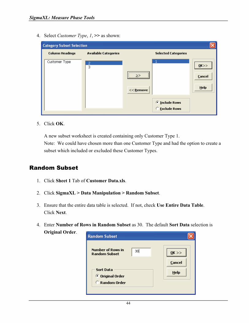
4. Select Customer Type, 1, >> as shown:
5. Click OK.
A new subset worksheet is created containing only Customer Type 1.
Note: We could have chosen more than one Customer Type and had the option to create a
subset which included or excluded these Customer Types.
Random Subset
1. Click Sheet 1 Tab of Customer Data.xls.
2. Click SigmaXL > Data Manipulation > Random Subset.
3. Ensure that the entire data table is selected. If not, check Use Entire Data Table.
Click Next.
4. Enter Number of Rows in Random Subset as 30. The default Sort Data selection is
Original Order.
44
SigmaXL: Measure Phase Tools
5. Click OK. A new worksheet is created that contains a random subset of 30 rows.
This feature is useful for data collection to ensure a random sample, e.g., given a list of
transaction numbers select a random sample of 30 transactions.
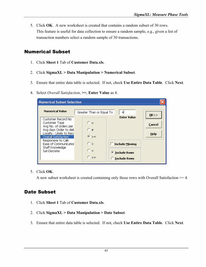
Numerical Subset
1. Click Sheet 1 Tab of Customer Data.xls.
2. Click SigmaXL > Data Manipulation > Numerical Subset.
3. Ensure that entire data table is selected. If not, check Use Entire Data Table. Click Next.
4. Select Overall Satisfaction, >=, Enter Value as 4.
5. Click OK.
A new subset worksheet is created containing only those rows with Overall Satisfaction >= 4.
Date Subset
1. Click Sheet 1 Tab of Customer Data.xls.
2. Click SigmaXL > Data Manipulation > Date Subset.
3. Ensure that entire data table is selected. If not, check Use Entire Data Table. Click Next.
45

SigmaXL: Measure Phase Tools
4. Select Order Date, select 1/9/2001, click Start Date, select 1/12/2001, click End Date.
5. Click OK. A new subset worksheet is created containing only those rows with Order Date
between 1/9/2001 to 1/12/2001.
Transpose Data
1. Open Catapult Data Row Format.xls.
2. Manually select the entire data table.
3. Click SigmaXL > Data Manipulation > Transpose Data.
4. This will transpose rows to columns or columns to rows. It is equivalent to Copy, Paste
Special, Transpose.
Stack Subgroups Across Rows
5. Now we will stack the subgroups across rows for the transposed data. Ensure that the
Transposed Data Sheet of Catapult Data Row Format.xls is active.
6. Click SigmaXL > Data Manipulation > Stack Subgroups Across Rows.
7. Check Use Entire Data Table, click Next.
8. Click on Shot 1. Shift Click on Shot 3 to highlight the three columns of interest.
46
SigmaXL: Measure Phase Tools
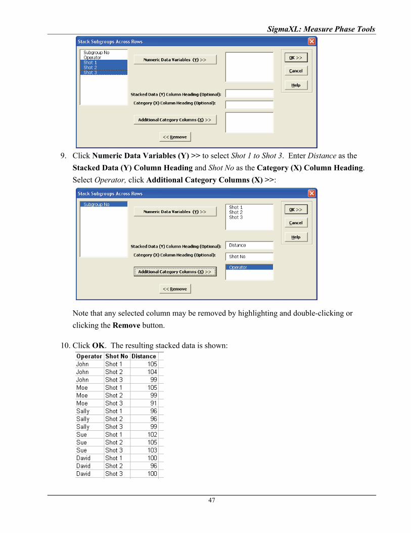
9. Click Numeric Data Variables (Y) >> to select Shot 1 to Shot 3. Enter Distance as the
Stacked Data (Y) Column Heading and Shot No as the Category (X) Column Heading.
Select Operator, click Additional Category Columns (X) >>:
Note that any selected column may be removed by highlighting and double-clicking or
clicking the Remove button.
10. Click OK. The resulting stacked data is shown:
47

SigmaXL: Measure Phase Tools
Stack Columns
1. Open Customer Satisfaction Unstacked.xls.
2. Click SigmaXL > Data Manipulation > Stack Columns.
3. Check Use Entire Data Table, click Next.
4. Shift Click on Overall Satisfaction_3 to highlight all three column names. Click Select
Columns >>. Enter the Stacked Data (Y) Column Name as Overall Satisfaction. Enter the
Category (X) Column Name as Customer Type.
5. Click OK. Shown is the resulting stacked column format:
6. Data that is in stacked column format can be unstacked using Data Manipulation > Unstack
Columns.
48

SigmaXL: Measure Phase Tools
Random Data
The normal random data generator is used to produce normal random data. Column headings are automatically created with Mean and Standard Deviation values (e.g. 1: Mean = 0; Stdev = 1). This utility works with Recall SigmaXL Dialog (F3) to append columns to the current Normal Random Data worksheet. An example is shown in Measure Phase Tools, Part G – Normal Probability Plots.
Additional random number generators include Uniform (Continuous & Integer), Lognormal, Exponential, Weibull and Triangular. The column headings show the specified parameter values.
Box-Cox Transformation This tool is used to convert non-normal data to normal by applying a power transformation. Examples of use are given in Measure Phase Tools, Part J – Process Capability for Non-Normal Data and Control Phase Tools, Part A – Individuals Charts for Non-Normal Data.
Standardize Data This tool is used to Standardize ((Yi – Mean)/StDev) or Code (Ymax = +1, Ymin = -1) your data. This is particularly useful when performing Multiple Regression. Standardized Predictors have better statistical properties. For example, the importance of model coefficients can be determined by the relative size because units are removed. Another statistical benefit is reduced multicollinearity when investigating two-factor interactions.
1. Click Sheet 1 Tab of Customer Data.xls.
2. Click SigmaXL > Data Manipulation > Standardize Data.
3. Ensure that the entire data table is selected. If not, check Use Entire Data Table.
Click Next.
4. Select Responsive to Calls and Ease of Communications and click Numeric (Y) Columns to
Standardize >>.
49
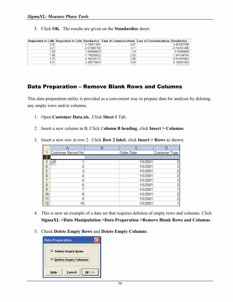
SigmaXL: Measure Phase Tools
5. Click OK. The results are given on the Standardize sheet:
Data Preparation – Remove Blank Rows and Columns
This data preparation utility is provided as a convenient way to prepare data for analysis by deleting
any empty rows and/or columns.
1. Open Customer Data.xls. Click Sheet 1 Tab.
2. Insert a new column in B; Click Column B heading, click Insert > Columns.
3. Insert a new row in row 2. Click Row 2 label, click Insert > Rows as shown:
4. This is now an example of a data set that requires deletion of empty rows and columns. Click
SigmaXL >Data Manipulation >Data Preparation >Remove Blank Rows and Columns.
5. Check Delete Empty Rows and Delete Empty Columns.
50
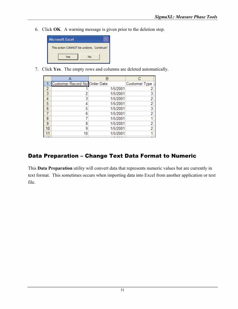
SigmaXL: Measure Phase Tools
6. Click OK. A warning message is given prior to the deletion step.
7. Click Yes. The empty rows and columns are deleted automatically.
Data Preparation – Change Text Data Format to Numeric
This Data Preparation utility will convert data that represents numeric values but are currently in
text format. This sometimes occurs when importing data into Excel from another application or text
file.
51

SigmaXL: Measure Phase Tools
Recall SigmaXL Dialog
Recall SigmaXL Dialog is used to activate the last data worksheet and recall the last dialog, making
it very easy to do repetitive analysis. To access, click the top level menu Recall SigmaXL Dialog
located to the right of the SigmaXL menu:
Alternatively, you can use the Hot Key F3. This feature can also be accessed by clicking SigmaXL
> Help > Hot Keys > Recall SigmaXL Dialog.
In Excel 2007/2010, the Recall SigmaXL Dialog menu button appears as:
Note that Recall SigmaXL Dialog may not be available for all functions.
Activate Last Worksheet
Activate Last Worksheet is used to activate the last data worksheet without recalling the dialog. To
access, press hot key F4. This feature can also be accessed by clicking SigmaXL > Help > Hot
Keys > Activate Last Sheet.
Worksheet Manager
The Worksheet Manager is a powerful utility that allows you to list all open Excel workbooks,
display all worksheets and chart sheets in a selected workbook and quickly select a worksheet or
chart sheet of interest. To access, click SigmaXL > Worksheet Manager.
52

SigmaXL: Measure Phase Tools
53
Part B – Templates & Calculators
Introduction to Templates & Calculators
To use SigmaXL templates, select the appropriate template, enter the inputs and the resulting outputs
are produced immediately. If the template does not automatically perform the calculations, click
Tools > Options, select Calculation, Automatic, and click OK (Excel 2007: Office Button | Excel
Options | Formulas, select Automatic, click OK; Excel 2010: File | Options…). Templates and
Calculators are protected worksheets by default, but this may be modified by clicking SigmaXL >
Help > Unprotect Worksheet. Alternatively, you can click Excel Tools > Protection > Unprotect
Sheet (Excel 2007/2010: Review | Changes | Unprotect Sheet). Gage R&R is password protected,
so it cannot be unprotected.
Click SigmaXL > Templates & Calculators to access the templates and calculators. Basic
Graphical Templates can also be accessed by clicking SigmaXL > Graphical Tools > Basic
Graphical Templates. Basic Statistical Templates can be accessed by clicking SigmaXL >
Statistical Tools > Basic Statistical Templates. Basic MSA Templates can be accessed by clicking
SigmaXL > Measurement Systems Analysis > Basic MSA Templates. Basic Process Capability
Templates can be accessed by clicking SigmaXL > Process Capability > Basic Process Capability
Templates. Basic DOE Templates can also be accessed by clicking SigmaXL > Design of
Experiments > Basic DOE Templates. Basic Control Chart Templates can also be accessed by
clicking SigmaXL > Control Charts > Basic Control Chart Templates.

SigmaXL: Measure Phase Tools
54
SigmaXL Templates & Calculators DMAIC & DFSS Templates:
o Team/Project Charter o SIPOC Diagram o Flowchart Toolbar o Data Measurement Plan o Cause & Effect (Fishbone) Diagram and Quick Template o Cause & Effect (XY) Matrix o Failure Mode & Effects Analysis (FMEA) o Quality Function Deployment (QFD) o Pugh Concept Selection Matrix o Control Plan
Lean Templates: o Takt Time Calculator o Value Analysis/Process Load Balance o Value Stream Mapping
Basic Graphical Templates: o Pareto Chart o Histogram o Run Chart
Basic Statistical Templates: o Sample Size – Discrete and Continuous o 1 Sample t Confidence Interval for Mean** o 2 Sample t-Test (Assume Equal and Unequal Variances) o 1 Sample Confidence Interval for Standard Deviation o 2 Sample F-Test (Compare 2 StDevs) o 1 Proportion Confidence Interval (Normal and Exact) o 2 Proportions Test & Fisher’s Exact
Probability Distribution Calculators: o Normal, Inverse Normal, Lognormal, Exponential, Weibull o Binomial, Poisson, Hypergeometric
Basic MSA Templates: o Gage R&R Study – with Multi-Vari Analysis o Attribute Gage R&R (Attribute Agreement Analysis)
•Basic Process Capability Templates: o Process Sigma Level – Discrete and Continuous o Process Capability & Confidence Intervals
Basic DOE Templates: o 2 to 5 Factors o Main Effects & Interaction Plots
Basic Control Chart Templates: o Individuals o C-Chart
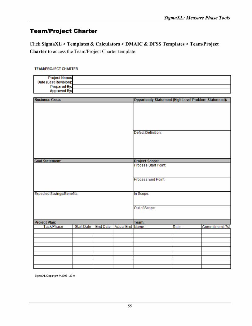
SigmaXL: Measure Phase Tools
Team/Project Charter
Click SigmaXL > Templates & Calculators > DMAIC & DFSS Templates > Team/Project
Charter to access the Team/Project Charter template.
55

SigmaXL: Measure Phase Tools
SIPOC Diagram
Click SigmaXL > Templates & Calculators > DMAIC & DFSS Templates > SIPOC Diagram to
access the SIPOC Diagram template.
Data Measurement Plan
Click SigmaXL > Templates & Calculators > DMAIC & DFSS Templates > Data
Measurement Plan to access the Data Measurement Plan template.
56
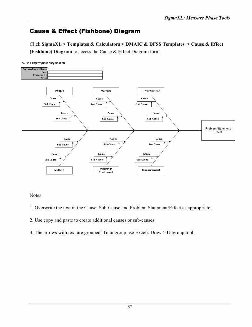
SigmaXL: Measure Phase Tools
Cause & Effect (Fishbone) Diagram
Click SigmaXL > Templates & Calculators > DMAIC & DFSS Templates > Cause & Effect
(Fishbone) Diagram to access the Cause & Effect Diagram form.
Notes:
1. Overwrite the text in the Cause, Sub-Cause and Problem Statement/Effect as appropriate.
2. Use copy and paste to create additional causes or sub-causes.
3. The arrows with text are grouped. To ungroup use Excel's Draw > Ungroup tool.
57
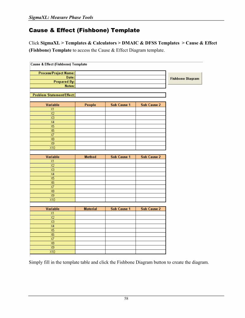
SigmaXL: Measure Phase Tools
Cause & Effect (Fishbone) Template
Click SigmaXL > Templates & Calculators > DMAIC & DFSS Templates > Cause & Effect
(Fishbone) Template to access the Cause & Effect Diagram template.
Simply fill in the template table and click the Fishbone Diagram button to create the diagram.
58

SigmaXL: Measure Phase Tools
Cause & Effect (XY) Matrix Example
Click SigmaXL > Templates & Calculators > DMAIC & DFSS Templates > Cause & Effect
(XY) Matrix to access the Cause & Effect (XY) Matrix template.
The following example is given in the file Template & Calculator Examples.xls. Click on the
worksheet named C&E Matrix. This is a simple Cause and Effect Matrix example for a Call
Center. If prompted, please ensure that macros are enabled in order to allow Pareto Charts to be
created.
Notes for use of the Cause and Effect Matrix template, also known as the XY Matrix:
1. Weight the Output Variables (Y's) on a scale of 1 to 10 with 10 indicating most important to
the Customer.
2. For Root Cause Analysis, assign the association/effect multiplier score for each X to Y using
a scale of 0, 1, 3, 9, where 0 = None, 1 = Weak, 3 = Moderate, and 9 = Strong. Initially this
assignment will likely be a team subjective assessment. Data should be collected and the
degree of association should be validated with Graphical and Statistical Tools.
3. For Project Selection or Solution Selection, assign the association multiplier score for each X
to Y using a scale of 1 to 10, with 10 indicating strong association.
Click the Pareto Chart button to
create a Pareto Chart of Weighted
Scores by Input/Process
Variables:
59

SigmaXL: Measure Phase Tools
Failure Mode & Effects Analysis (FMEA) Example
Click SigmaXL > Templates & Calculators > DMAIC & DFSS Templates > Failure Mode &
Effects Analysis (FMEA) template.
The following example is given in the file Template & Calculator Examples.xls. Click on the
worksheet named FMEA. This is a simple Failure Mode and Effects example for Stocking
Inventory. If prompted, please ensure that macros are enabled in order to allow sort by RPN.
If you hover the mouse cursor over the Severity, Occurrence or Detection heading the
recommended scale will appear as a comment:
60
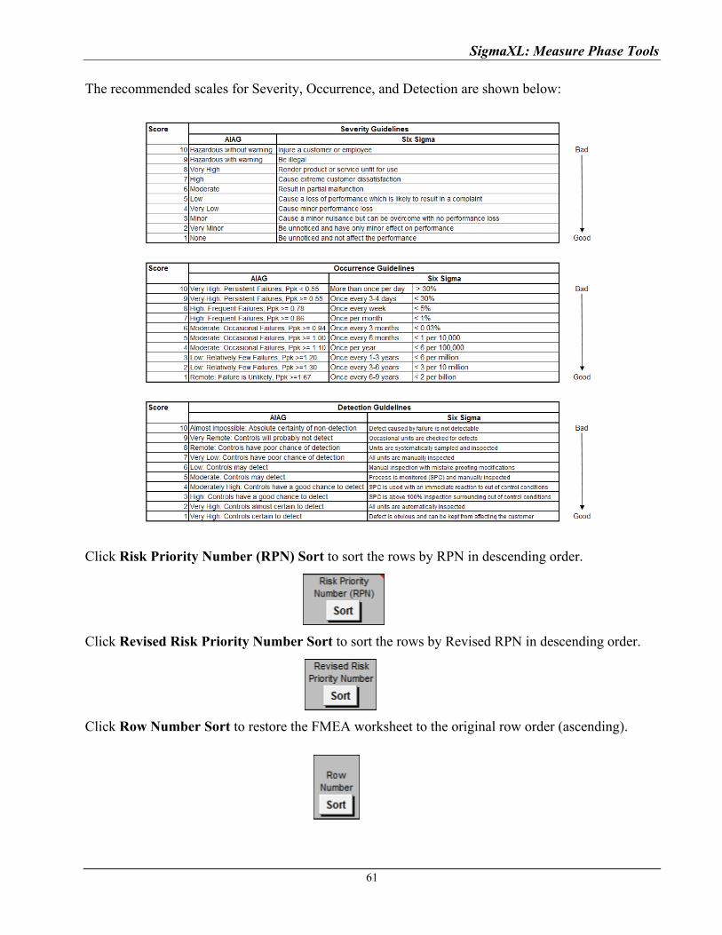
SigmaXL: Measure Phase Tools
The recommended scales for Severity, Occurrence, and Detection are shown below:
Click Risk Priority Number (RPN) Sort to sort the rows by RPN in descending order.
Click Revised Risk Priority Number Sort to sort the rows by Revised RPN in descending order.
Click Row Number Sort to restore the FMEA worksheet to the original row order (ascending).
61
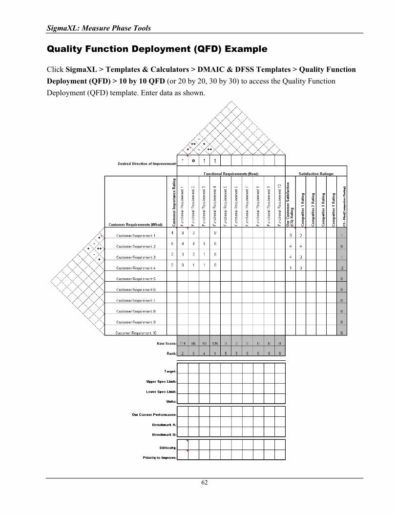
SigmaXL: Measure Phase Tools
Quality Function Deployment (QFD) Example
Click SigmaXL > Templates & Calculators > DMAIC & DFSS Templates > Quality Function
Deployment (QFD) > 10 by 10 QFD (or 20 by 20, 30 by 30) to access the Quality Function
Deployment (QFD) template. Enter data as shown.
62

SigmaXL: Measure Phase Tools
Pugh Concept Selection Matrix Example
Click SigmaXL > Templates & Calculators > DMAIC & DFSS Templates > Pugh Concept
Selection Matrix to access the Pugh Concept Selection Matrix template. Enter data as shown.
63
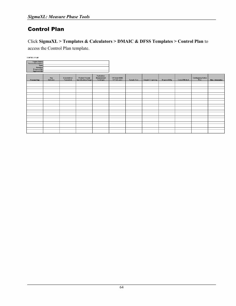
SigmaXL: Measure Phase Tools
Control Plan
Click SigmaXL > Templates & Calculators > DMAIC & DFSS Templates > Control Plan to
access the Control Plan template.
64
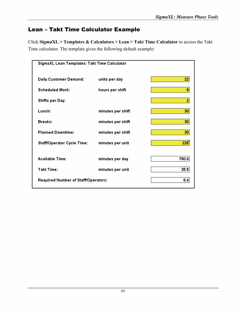
SigmaXL: Measure Phase Tools
Lean – Takt Time Calculator Example
Click SigmaXL > Templates & Calculators > Lean > Takt Time Calculator to access the Takt
Time calculator. The template gives the following default example:
65
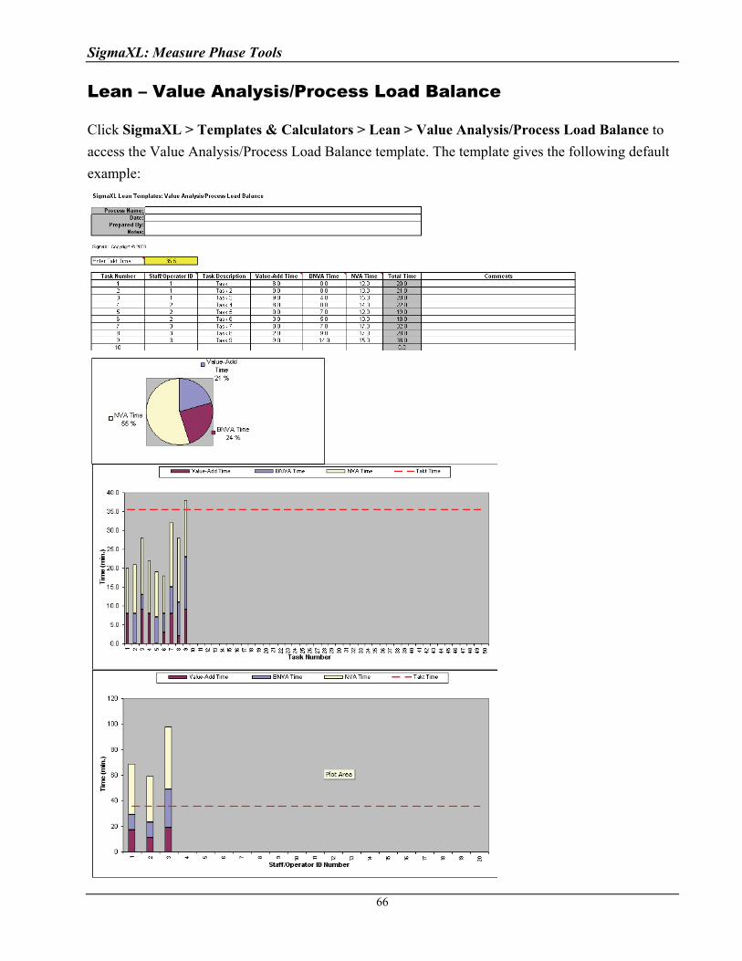
SigmaXL: Measure Phase Tools
Lean – Value Analysis/Process Load Balance
Click SigmaXL > Templates & Calculators > Lean > Value Analysis/Process Load Balance to
access the Value Analysis/Process Load Balance template. The template gives the following default
example:
66
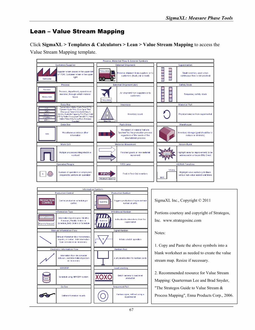
SigmaXL: Measure Phase Tools
Lean – Value Stream Mapping
Click SigmaXL > Templates & Calculators > Lean > Value Stream Mapping to access the
Value Stream Mapping template.
Notes:
1. Copy and Paste the above symbols into a
blank worksheet as needed to create the value
stream map. Resize if necessary.
2. Recommended resource for Value Stream
Mapping: Quarterman Lee and Brad Snyder,
"The Strategos Guide to Value Stream &
Process Mapping", Enna Products Corp., 2006.
Portions courtesy and copyright of Strategos,
Inc. www.strategosinc.com
SigmaXL Inc., Copyright © 2011
67
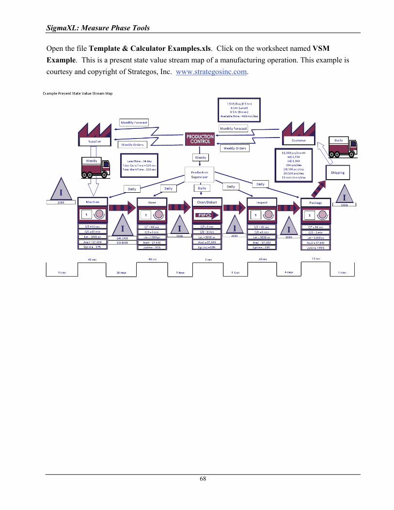
SigmaXL: Measure Phase Tools
Open the file Template & Calculator Examples.xls. Click on the worksheet named VSM
Example. This is a present state value stream map of a manufacturing operation. This example is
courtesy and copyright of Strategos, Inc. www.strategosinc.com.
68

SigmaXL: Measure Phase Tools
Basic Graphical Templates – Pareto Example
Click SigmaXL > Templates & Calculators > Basic Graphical Templates > Pareto Chart. Enter
data as shown:
Click the Pareto Chart button to produce the Pareto Chart:
Pareto Chart
0
10
20
30
40
50
60
70
80
90
100
Return-ca
lls
Difficu
lt-to-o
rder
Order
-take
s-too
-long
Wro
ng-co
lor
Not-ava
ilable
Category
Co
un
t
0%
10%
20%
30%
40%
50%
60%
70%
80%
90%
100%
Notes:
1. This Pareto Chart template should be used with count data like number of errors. You can
also create Pareto charts with cost data.
2. You can replace the Category and Count column headings with any headings that you wish.
3. Enter the Pareto categories in the Category column. These can be Name, Location, Error
Type or other text information. Pareto categories are required and will appear on the
horizontal X-Axis of the Pareto Chart.
4. Enter your count (or cost) data in the Count column.
5. Click the Pareto Chart button to create a Pareto Chart.
69
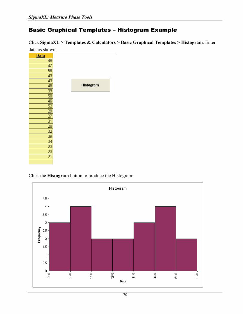
SigmaXL: Measure Phase Tools
Basic Graphical Templates – Histogram Example
Click SigmaXL > Templates & Calculators > Basic Graphical Templates > Histogram. Enter
data as shown:
Click the Histogram button to produce the Histogram:
70
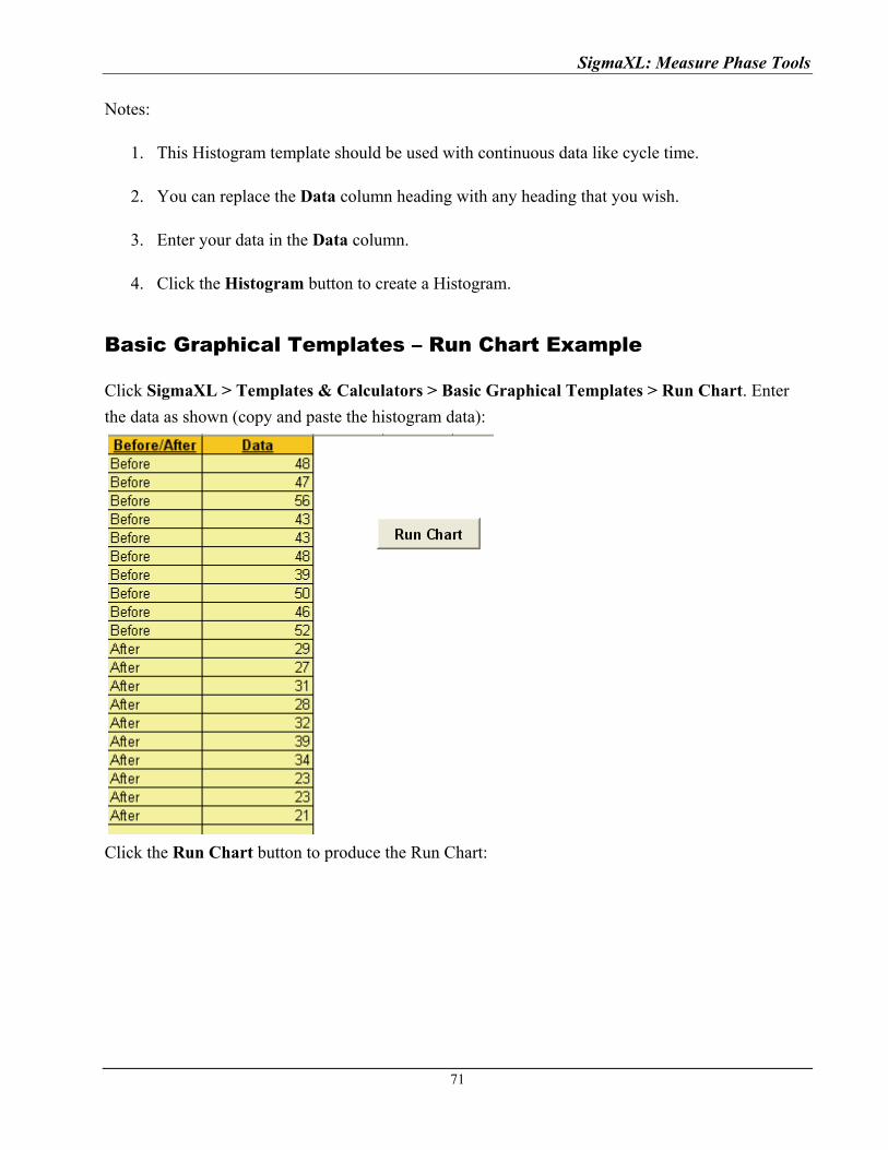
SigmaXL: Measure Phase Tools
Notes:
1. This Histogram template should be used with continuous data like cycle time.
2. You can replace the Data column heading with any heading that you wish.
3. Enter your data in the Data column.
4. Click the Histogram button to create a Histogram.
Basic Graphical Templates – Run Chart Example
Click SigmaXL > Templates & Calculators > Basic Graphical Templates > Run Chart. Enter
the data as shown (copy and paste the histogram data):
Click the Run Chart button to produce the Run Chart:
71

SigmaXL: Measure Phase Tools
Run Chart
Mean: 37.95
0
10
20
30
40
50
60
Befor
e
Befor
e
Befor
e
Befor
e
Befor
eAfte
rAfte
rAfte
rAfte
rAfte
r
Ru
n C
har
t: D
ata
Notes:
1. This Run Chart template can be used with a variety of data types: continuous data like cycle
time, count data like number of errors, or cost data. The data must be in chronological time-
sequence order.
2. You can replace the X-Axis Label and Data column headings with any headings that you
wish.
3. Enter your data in the Data column.
4. Enter labels in X-Axis Label column. Labels can be Date, Time, Name, or other text
information. These labels are optional and will appear on the horizontal X-Axis of the Run
Chart.
5. Click the Run Chart button to create a Run Chart.
72
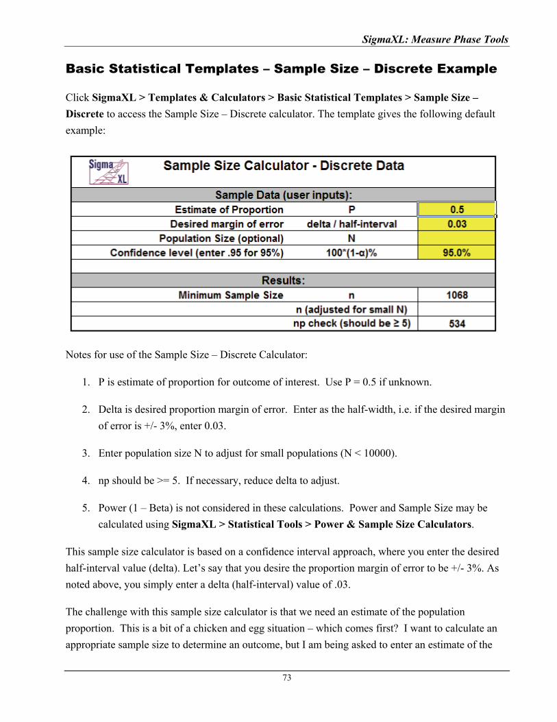
SigmaXL: Measure Phase Tools
Basic Statistical Templates – Sample Size – Discrete Example
Click SigmaXL > Templates & Calculators > Basic Statistical Templates > Sample Size –
Discrete to access the Sample Size – Discrete calculator. The template gives the following default
example:
Notes for use of the Sample Size – Discrete Calculator:
1. P is estimate of proportion for outcome of interest. Use P = 0.5 if unknown.
2. Delta is desired proportion margin of error. Enter as the half-width, i.e. if the desired margin
of error is +/- 3%, enter 0.03.
3. Enter population size N to adjust for small populations (N < 10000).
4. np should be >= 5. If necessary, reduce delta to adjust.
5. Power (1 – Beta) is not considered in these calculations. Power and Sample Size may be
calculated using SigmaXL > Statistical Tools > Power & Sample Size Calculators.
This sample size calculator is based on a confidence interval approach, where you enter the desired
half-interval value (delta). Let’s say that you desire the proportion margin of error to be +/- 3%. As
noted above, you simply enter a delta (half-interval) value of .03.
The challenge with this sample size calculator is that we need an estimate of the population
proportion. This is a bit of a chicken and egg situation – which comes first? I want to calculate an
appropriate sample size to determine an outcome, but I am being asked to enter an estimate of the
73

SigmaXL: Measure Phase Tools
74
population proportion. First, keep in mind that this tool is a planning tool – the true confidence
intervals will be determined after you collect your data. Estimating the population proportion can be
done if you have good historical data to draw from, for example, in historical customer surveys the
percentage of satisfied customers was 80%. In this case you could use P=0.8. If you do not have a
priori knowledge, then leave P=0.5 which gives the most conservative value (i.e., largest estimate of
sample size). If you enter a value other than 0.5 it will result in a smaller sample size requirement.
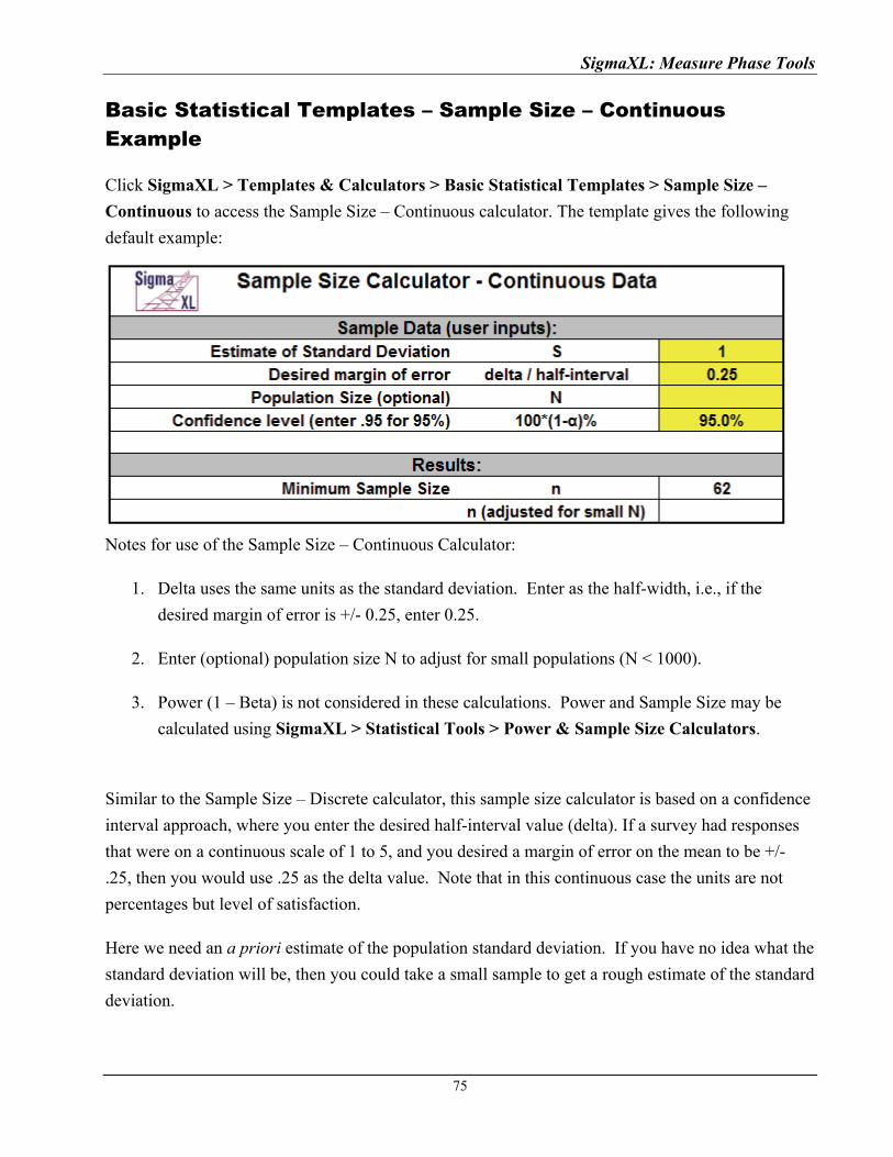
SigmaXL: Measure Phase Tools
Basic Statistical Templates – Sample Size – Continuous Example
Click SigmaXL > Templates & Calculators > Basic Statistical Templates > Sample Size –
Continuous to access the Sample Size – Continuous calculator. The template gives the following
default example:
Notes for use of the Sample Size – Continuous Calculator:
1. Delta uses the same units as the standard deviation. Enter as the half-width, i.e., if the
desired margin of error is +/- 0.25, enter 0.25.
2. Enter (optional) population size N to adjust for small populations (N < 1000).
3. Power (1 – Beta) is not considered in these calculations. Power and Sample Size may be
calculated using SigmaXL > Statistical Tools > Power & Sample Size Calculators.
Similar to the Sample Size – Discrete calculator, this sample size calculator is based on a confidence
interval approach, where you enter the desired half-interval value (delta). If a survey had responses
that were on a continuous scale of 1 to 5, and you desired a margin of error on the mean to be +/-
.25, then you would use .25 as the delta value. Note that in this continuous case the units are not
percentages but level of satisfaction.
Here we need an a priori estimate of the population standard deviation. If you have no idea what the
standard deviation will be, then you could take a small sample to get a rough estimate of the standard
deviation.
75

SigmaXL: Measure Phase Tools
Basic Statistical Templates – 1 Sample t Confidence Interval for Mean Example
Click SigmaXL > Templates & Calculators > Basic Statistical Templates > 1 Sample t
Confidence Interval for Mean to access the 1 Sample t Confidence Interval for Mean calculator.
The template gives the following default example.
76

SigmaXL: Measure Phase Tools
Basic Statistical Templates – 2 Sample t-Test (Assume Equal Variance) Example
Click SigmaXL > Templates & Calculators > Basic Statistical Templates > 2 Sample t-Test
(Assume Equal Variances) to access the 2 Sample t-Test calculator. The template gives the
following default example.
Basic Statistical Templates – 2 Sample t-Test (Assume Unequal Variance) Example
Click SigmaXL > Templates & Calculators > Basic Statistical Templates > 2 Sample t-Test
(Assume Unequal Variances) to access the 2 Sample t-Test calculator. The template gives the
following default example.
77
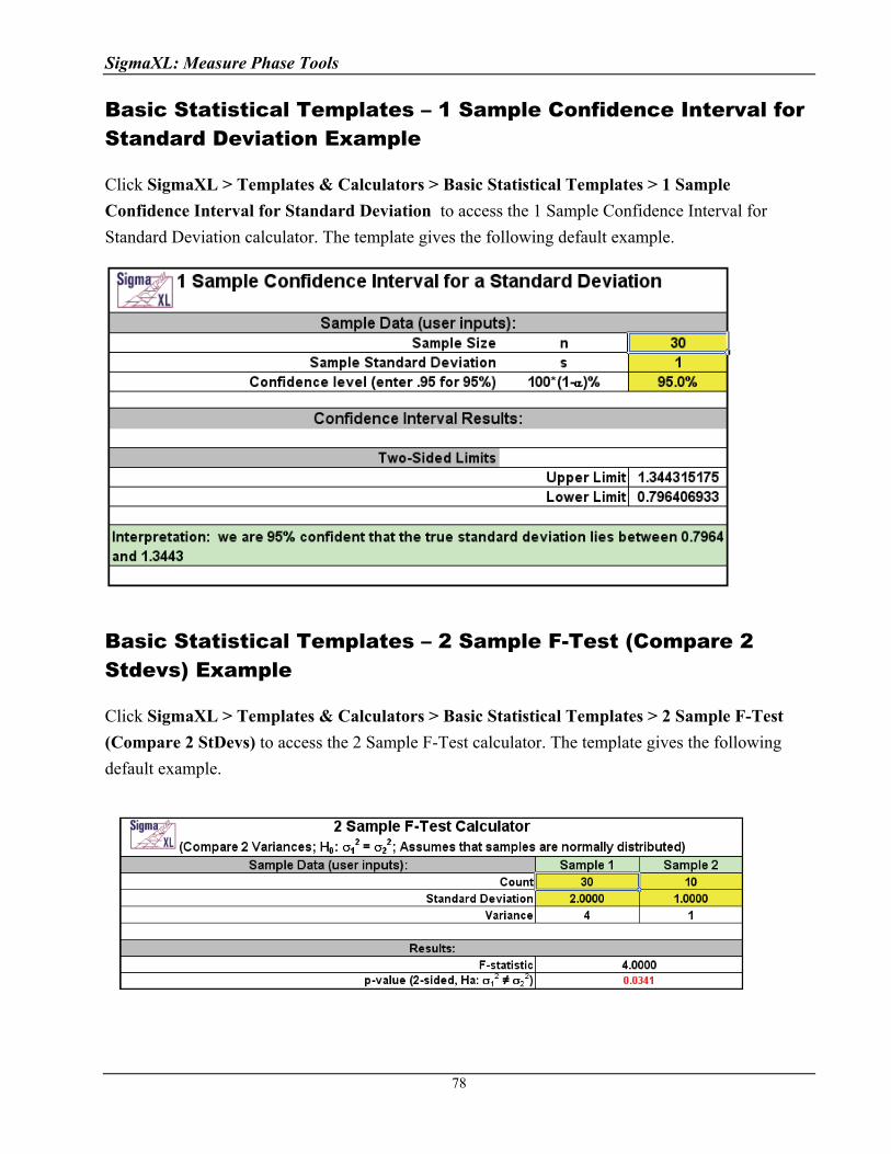
SigmaXL: Measure Phase Tools
Basic Statistical Templates – 1 Sample Confidence Interval for Standard Deviation Example
Click SigmaXL > Templates & Calculators > Basic Statistical Templates > 1 Sample
Confidence Interval for Standard Deviation to access the 1 Sample Confidence Interval for
Standard Deviation calculator. The template gives the following default example.
Basic Statistical Templates – 2 Sample F-Test (Compare 2 Stdevs) Example
Click SigmaXL > Templates & Calculators > Basic Statistical Templates > 2 Sample F-Test
(Compare 2 StDevs) to access the 2 Sample F-Test calculator. The template gives the following
default example.
78
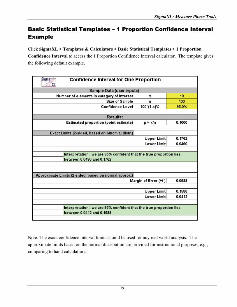
SigmaXL: Measure Phase Tools
Basic Statistical Templates – 1 Proportion Confidence Interval Example
Click SigmaXL > Templates & Calculators > Basic Statistical Templates > 1 Proportion
Confidence Interval to access the 1 Proportion Confidence Interval calculator. The template gives
the following default example.
Note: The exact confidence interval limits should be used for any real world analysis. The
approximate limits based on the normal distribution are provided for instructional purposes, e.g.,
comparing to hand calculations.
79
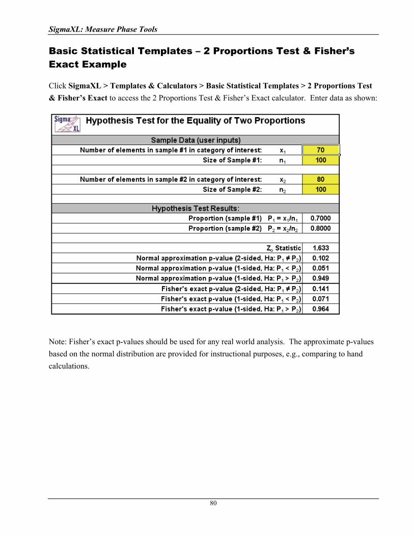
SigmaXL: Measure Phase Tools
Basic Statistical Templates – 2 Proportions Test & Fisher’s Exact Example
Click SigmaXL > Templates & Calculators > Basic Statistical Templates > 2 Proportions Test
& Fisher’s Exact to access the 2 Proportions Test & Fisher’s Exact calculator. Enter data as shown:
Note: Fisher’s exact p-values should be used for any real world analysis. The approximate p-values
based on the normal distribution are provided for instructional purposes, e.g., comparing to hand
calculations.
80

SigmaXL: Measure Phase Tools
Probability Distribution Calculators – Normal Example
Click SigmaXL > Templates & Calculators > Probability Distribution Calculators > Normal to
access the Normal Distribution Probability calculator. The template gives the following default
example:
81
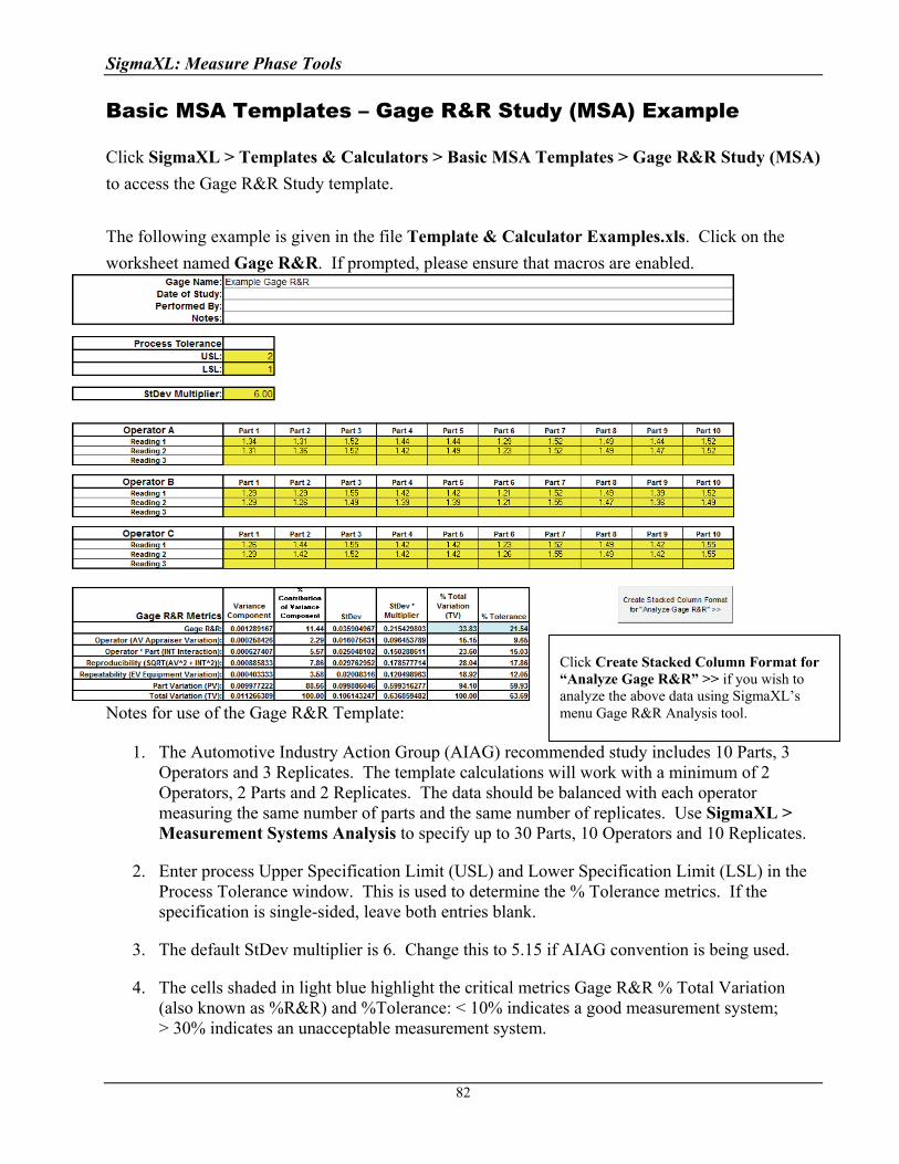
SigmaXL: Measure Phase Tools
Basic MSA Templates – Gage R&R Study (MSA) Example
Click SigmaXL > Templates & Calculators > Basic MSA Templates > Gage R&R Study (MSA)
to access the Gage R&R Study template.
The following example is given in the file Template & Calculator Examples.xls. Click on the
worksheet named Gage R&R. If prompted, please ensure that macros are enabled.
Notes for use of the Gage R&R Template:
1. The Automotive Industry Action Group (AIAG) recommended study includes 10 Parts, 3 Operators and 3 Replicates. The template calculations will work with a minimum of 2 Operators, 2 Parts and 2 Replicates. The data should be balanced with each operator measuring the same number of parts and the same number of replicates. Use SigmaXL > Measurement Systems Analysis to specify up to 30 Parts, 10 Operators and 10 Replicates.
Click Create Stacked Column Format for “Analyze Gage R&R” >> if you wish to analyze the above data using SigmaXL’s menu Gage R&R Analysis tool.
2. Enter process Upper Specification Limit (USL) and Lower Specification Limit (LSL) in the Process Tolerance window. This is used to determine the % Tolerance metrics. If the specification is single-sided, leave both entries blank.
3. The default StDev multiplier is 6. Change this to 5.15 if AIAG convention is being used.
4. The cells shaded in light blue highlight the critical metrics Gage R&R % Total Variation (also known as %R&R) and %Tolerance: < 10% indicates a good measurement system; > 30% indicates an unacceptable measurement system.
82
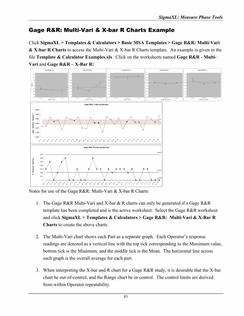
SigmaXL: Measure Phase Tools
Gage R&R: Multi-Vari & X-bar R Charts Example
Click SigmaXL > Templates & Calculators > Basic MSA Templates > Gage R&R: Multi-Vari
& X-bar R Charts to access the Multi-Vari & X-bar R Charts template. An example is given in the
file Template & Calculator Examples.xls. Click on the worksheets named Gage R&R - Multi-
Vari and Gage R&R – X-Bar R:
83
Notes for use of the Gage R&R: Multi-Vari & X-bar R Charts:
Gage R&R Multi-Vari
1.1685
1.2185
1.2685
1.3185
1.3685
1.4185
1.4685
1.5185
1.5685
Operator A Operator B Operator C
Operator - Part 01
Rea
din
g
Gage R&R Multi-Vari
1.1685
1.2185
1.2685
1.3185
1.3685
1.4185
1.4685
1.5185
1.5685
Operator A Operator B Operator C
Operator - Part 02
Gage R&R Multi-Vari
1.1685
1.2185
1.2685
1.3185
1.3685
1.4185
1.4685
1.5185
1.5685
Operator A Operator B Operator C
Operator - Part 03
Gage R&R Multi-Vari
1.1685
1.2185
1.2685
1.3185
1.3685
1.4185
1.4685
1.5185
1.5685
Operator A Operator B Operator C
Operator - Part: Part 04
Gage R&R Multi-Vari
1.1685
1.2185
1.2685
1.3185
1.3685
1.4185
1.4685
1.5185
1.5685
Operator A Operator B Operator C
Operator - Part: Part 05
Gage R&R - X-Bar by Operator
1.38
1.42
1.46
1.0890
1.1890
1.2890
1.3890
1.4890
1.5890
1.6890
A - 1
A - 2
A - 3
A - 4
A - 5
A - 6
A - 7
A - 8
A - 9
A - 10
B - 1
B - 2
B - 3
B - 4
B - 5
B - 6
B - 7
B - 8
B - 9
B - 10
C - 1
C - 2
C - 3
C - 4
C - 5
C - 6
C - 7
C - 8
C - 9
C - 10
X-B
ar -
Rea
din
g1
- R
ead
ing
3
Gage R&R - R-Chart by Operator
0.00000
0.02133
0.06970
0
0.01
0.02
0.03
0.04
0.05
0.06
0.07
A - 1
A - 2
A - 3
A - 4
A - 5
A - 6
A - 7
A - 8
A - 9
A - 10
B - 1
B - 2
B - 3
B - 4
B - 5
B - 6
B - 7
B - 8
B - 9
B - 10
C - 1
C - 2
C - 3
C - 4
C - 5
C - 6
C - 7
C - 8
C - 9
C - 10
R -
Rea
din
g1
- R
ead
ing
3
1. The Gage R&R Multi-Vari and X-bar & R charts can only be generated if a Gage R&R
template has been completed and is the active worksheet. Select the Gage R&R worksheet
and click SigmaXL > Templates & Calculators > Gage R&R: Multi-Vari & X-Bar R
Charts to create the above charts.
2. The Multi-Vari chart shows each Part as a separate graph. Each Operator’s response
readings are denoted as a vertical line with the top tick corresponding to the Maximum value,
bottom tick is the Minimum, and the middle tick is the Mean. The horizontal line across
each graph is the overall average for each part.
3. When interpreting the X-bar and R chart for a Gage R&R study, it is desirable that the X-bar
chart be out-of-control, and the Range chart be in-control. The control limits are derived
from within Operator repeatability.
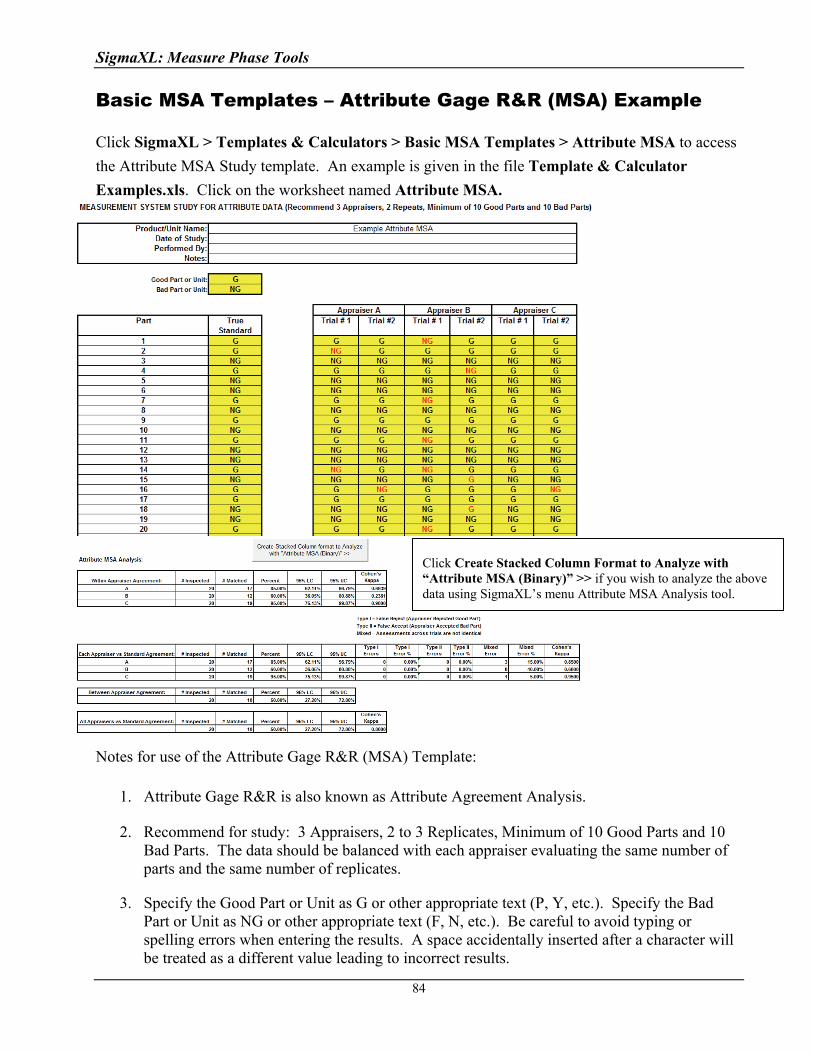
SigmaXL: Measure Phase Tools
Basic MSA Templates – Attribute Gage R&R (MSA) Example
Click SigmaXL > Templates & Calculators > Basic MSA Templates > Attribute MSA to access
the Attribute MSA Study template. An example is given in the file Template & Calculator
Examples.xls. Click on the worksheet named Attribute MSA.
Notes for use of the Attribute Gage R&R (MSA) Template:
Click Create Stacked Column Format to Analyze with “Attribute MSA (Binary)” >> if you wish to analyze the above data using SigmaXL’s menu Attribute MSA Analysis tool.
1. Attribute Gage R&R is also known as Attribute Agreement Analysis.
2. Recommend for study: 3 Appraisers, 2 to 3 Replicates, Minimum of 10 Good Parts and 10 Bad Parts. The data should be balanced with each appraiser evaluating the same number of parts and the same number of replicates.
3. Specify the Good Part or Unit as G or other appropriate text (P, Y, etc.). Specify the Bad Part or Unit as NG or other appropriate text (F, N, etc.). Be careful to avoid typing or spelling errors when entering the results. A space accidentally inserted after a character will be treated as a different value leading to incorrect results.
84

SigmaXL: Measure Phase Tools
Basic Process Capability Templates – Process Sigma Level – Discrete Data Example
Click SigmaXL > Templates & Calculators > Basic Process Capability Templates > Process
Sigma Level – Discrete to access the Process Sigma Level – Discrete calculator. The template
gives the following default example.
Notes for use of the Process Sigma Calculator for Discrete Data:
1. Total number of defects should include defects made and later fixed.
2. Sample size should be large enough to observe 5 defects.
85
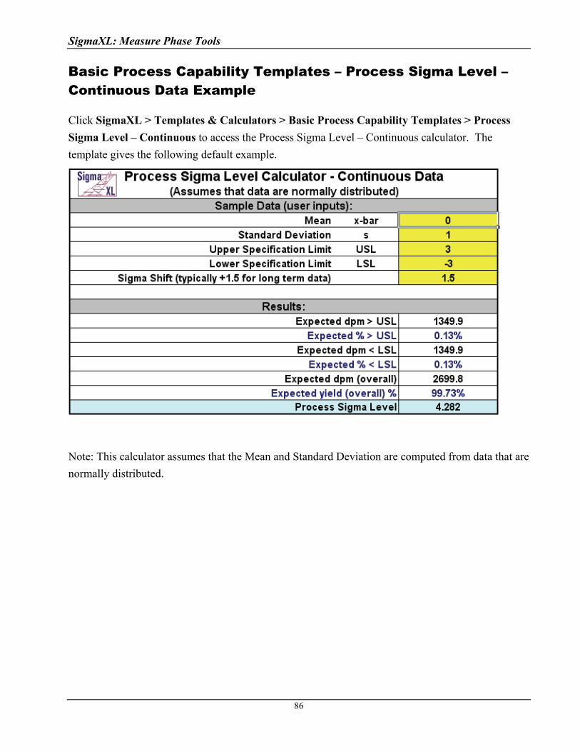
SigmaXL: Measure Phase Tools
Basic Process Capability Templates – Process Sigma Level – Continuous Data Example
Click SigmaXL > Templates & Calculators > Basic Process Capability Templates > Process
Sigma Level – Continuous to access the Process Sigma Level – Continuous calculator. The
template gives the following default example.
Note: This calculator assumes that the Mean and Standard Deviation are computed from data that are
normally distributed.
86

SigmaXL: Measure Phase Tools
Basic Process Capability Templates – Process Capability Indices Example
Click SigmaXL > Templates & Calculators > Basic Process Capability Templates > Process
Capability to access the Process Capability Indices calculator. The template gives the following
default example.
Notes for use of the Process Capability Indices Calculator:
1. This calculator assumes that the Mean and Standard Deviation are computed from data that
are normally distributed.
2. Reports Cp, Cpk if entered S is Within or Short Term (using a control chart).
3. Reports Pp, Ppk if entered S is Overall or Long Term.
87

SigmaXL: Measure Phase Tools
Basic Process Capability Templates – Process Capability & Confidence Intervals Example
Click SigmaXL > Templates & Calculators > Basic Process Capability Templates > Process
Capability & Confidence Intervals to access the Process Capability Indices & Confidence
Intervals calculator. The template gives the following default example.
Notes for use of the Process Capability & Confidence Intervals Calculator:
1. This calculator assumes that the Mean and Standard Deviation are computed from data that
are normally distributed.
2. Reports Cp, Cpk if entered S is Within or Short Term (using a control chart).
3. Reports Pp, Ppk if entered S is Overall or Long Term.
88
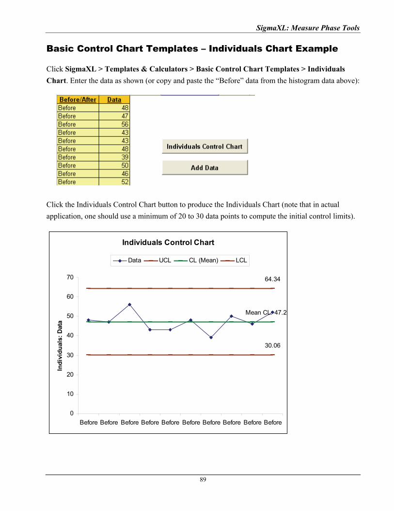
SigmaXL: Measure Phase Tools
Basic Control Chart Templates – Individuals Chart Example
Click SigmaXL > Templates & Calculators > Basic Control Chart Templates > Individuals
Chart. Enter the data as shown (or copy and paste the “Before” data from the histogram data above):
Click the Individuals Control Chart button to produce the Individuals Chart (note that in actual
application, one should use a minimum of 20 to 30 data points to compute the initial control limits).
Individuals Control Chart
64.34
Mean CL: 47.2
30.06
0
10
20
30
40
50
60
70
Before Before Before Before Before Before Before Before Before Before
Ind
ivid
ual
s: D
ata
Data UCL CL (Mean) LCL
89

SigmaXL: Measure Phase Tools
Now enter the data as shown (or copy and paste the “After” data from the histogram data used
earlier):
Click the Add Data button to add the “After” data to the Individuals chart.
Individuals Control Chart
64.34
Mean CL: 47.2
30.06
0
10
20
30
40
50
60
70
Befor
e
Befor
e
Befor
e
Befor
e
Befor
eAfte
rAfte
rAfte
rAfte
rAfte
r
Ind
ivid
ual
s: D
ata
Data UCL CL (Mean) LCL
90
SigmaXL: Measure Phase Tools
91
Notes:
1. This Individuals Control Chart template should be used with continuous data like cycle time.
The data must be in chronological time-sequence order.
2. You can replace the X-Axis Label and Data column headings with any headings that you
wish.
3. Enter your data in the Data column.
4. Enter labels in X-Axis Label column. Labels can be Date, Time, Name, or other text
information. These labels are optional and will appear on the horizontal X-Axis of the
Individuals Control Chart.
5. Click the Individuals Control Chart button to create an Individuals Control Chart.
6. After the control chart has been created and additional new data entered into the Data
column, click the Add Data button to add the data to the existing chart.
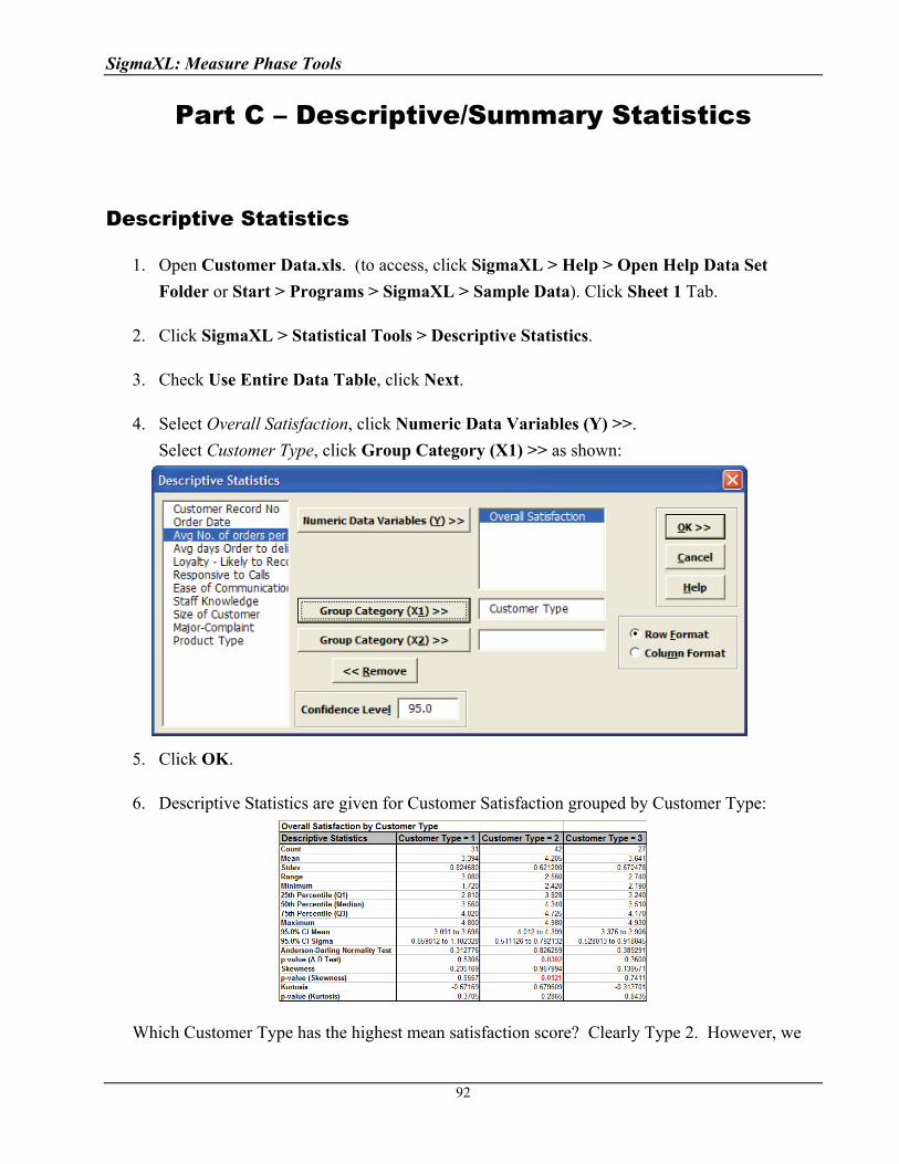
SigmaXL: Measure Phase Tools
Part C – Descriptive/Summary Statistics
Descriptive Statistics
1. Open Customer Data.xls. (to access, click SigmaXL > Help > Open Help Data Set
Folder or Start > Programs > SigmaXL > Sample Data). Click Sheet 1 Tab.
2. Click SigmaXL > Statistical Tools > Descriptive Statistics.
3. Check Use Entire Data Table, click Next.
4. Select Overall Satisfaction, click Numeric Data Variables (Y) >>.
Select Customer Type, click Group Category (X1) >> as shown:
5. Click OK.
6. Descriptive Statistics are given for Customer Satisfaction grouped by Customer Type:
Which Customer Type has the highest mean satisfaction score? Clearly Type 2. However, we
92
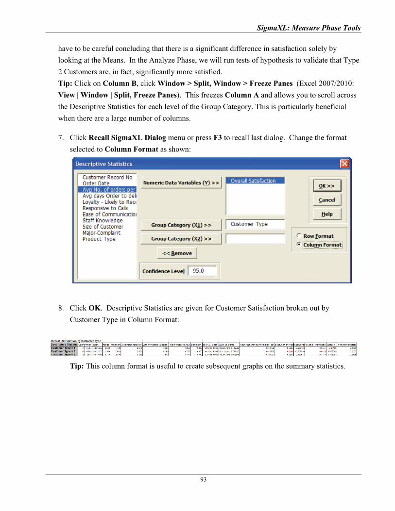
SigmaXL: Measure Phase Tools
have to be careful concluding that there is a significant difference in satisfaction solely by
looking at the Means. In the Analyze Phase, we will run tests of hypothesis to validate that Type
2 Customers are, in fact, significantly more satisfied.
Tip: Click on Column B, click Window > Split, Window > Freeze Panes (Excel 2007/2010:
View | Window | Split, Freeze Panes). This freezes Column A and allows you to scroll across
the Descriptive Statistics for each level of the Group Category. This is particularly beneficial
when there are a large number of columns.
7. Click Recall SigmaXL Dialog menu or press F3 to recall last dialog. Change the format
selected to Column Format as shown:
8. Click OK. Descriptive Statistics are given for Customer Satisfaction broken out by
Customer Type in Column Format:
Tip: This column format is useful to create subsequent graphs on the summary statistics.
93
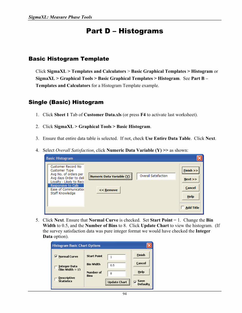
SigmaXL: Measure Phase Tools
Part D – Histograms
Basic Histogram Template
Click SigmaXL > Templates and Calculators > Basic Graphical Templates > Histogram or
SigmaXL > Graphical Tools > Basic Graphical Templates > Histogram. See Part B –
Templates and Calculators for a Histogram Template example.
Single (Basic) Histogram
1. Click Sheet 1 Tab of Customer Data.xls (or press F4 to activate last worksheet).
2. Click SigmaXL > Graphical Tools > Basic Histogram.
3. Ensure that entire data table is selected. If not, check Use Entire Data Table. Click Next.
4. Select Overall Satisfaction, click Numeric Data Variable (Y) >> as shown:
5. Click Next. Ensure that Normal Curve is checked. Set Start Point = 1. Change the Bin
Width to 0.5, and the Number of Bins to 8. Click Update Chart to view the histogram. (If the survey satisfaction data was pure integer format we would have checked the Integer Data option).
94
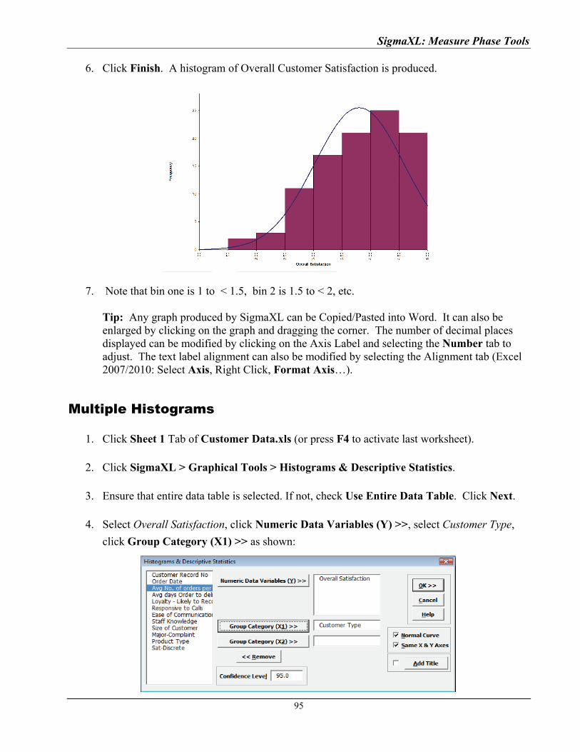
SigmaXL: Measure Phase Tools
6. Click Finish. A histogram of Overall Customer Satisfaction is produced.
7. Note that bin one is 1 to < 1.5, bin 2 is 1.5 to < 2, etc. Tip: Any graph produced by SigmaXL can be Copied/Pasted into Word. It can also be enlarged by clicking on the graph and dragging the corner. The number of decimal places displayed can be modified by clicking on the Axis Label and selecting the Number tab to adjust. The text label alignment can also be modified by selecting the Alignment tab (Excel 2007/2010: Select Axis, Right Click, Format Axis…).
Multiple Histograms
1. Click Sheet 1 Tab of Customer Data.xls (or press F4 to activate last worksheet).
2. Click SigmaXL > Graphical Tools > Histograms & Descriptive Statistics.
3. Ensure that entire data table is selected. If not, check Use Entire Data Table. Click Next.
4. Select Overall Satisfaction, click Numeric Data Variables (Y) >>, select Customer Type,
click Group Category (X1) >> as shown:
95

SigmaXL: Measure Phase Tools
5. Click OK. Multiple Histograms and Descriptive Statistics of Customer Satisfaction By
Customer Type are produced:
Clearly Customer Type 2 shows a higher level of overall satisfaction, with the data skewed
left. Note that Customer Type 1 and 3 have data that is normally distributed, but this is not
desirable when the response is a satisfaction score!
6. Note that bin one is 1.72 to < 1.99, bin 2 is 1.99 to < 2.26, etc. The number of decimals
displayed can be changed by double-clicking on the X axis, click Number tab, and adjust
decimal places.
96
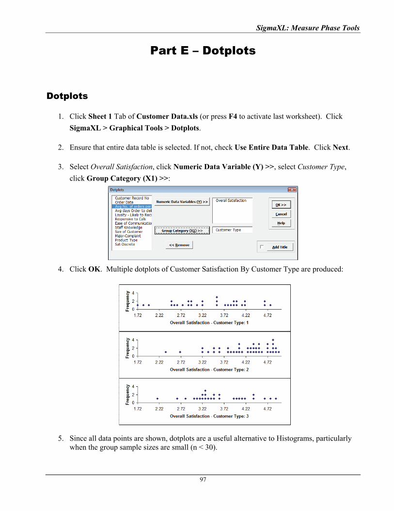
SigmaXL: Measure Phase Tools
Part E – Dotplots
Dotplots
1. Click Sheet 1 Tab of Customer Data.xls (or press F4 to activate last worksheet). Click
SigmaXL > Graphical Tools > Dotplots.
2. Ensure that entire data table is selected. If not, check Use Entire Data Table. Click Next.
3. Select Overall Satisfaction, click Numeric Data Variable (Y) >>, select Customer Type,
click Group Category (X1) >>:
4. Click OK. Multiple dotplots of Customer Satisfaction By Customer Type are produced:
5. Since all data points are shown, dotplots are a useful alternative to Histograms, particularly when the group sample sizes are small (n < 30).
97
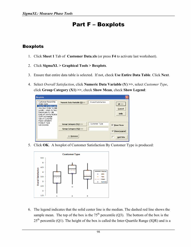
SigmaXL: Measure Phase Tools
Part F – Boxplots
Boxplots
1. Click Sheet 1 Tab of Customer Data.xls (or press F4 to activate last worksheet).
2. Click SigmaXL > Graphical Tools > Boxplots.
3. Ensure that entire data table is selected. If not, check Use Entire Data Table. Click Next.
4. Select Overall Satisfaction, click Numeric Data Variable (Y) >>, select Customer Type,
click Group Category (X1) >>, check Show Mean, check Show Legend:
5. Click OK. A boxplot of Customer Satisfaction By Customer Type is produced:
6. The legend indicates that the solid center line is the median. The dashed red line shows the
sample mean. The top of the box is the 75th percentile (Q3). The bottom of the box is the
25th percentile (Q1). The height of the box is called the Inter-Quartile Range (IQR) and is a
98
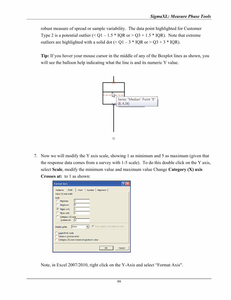
SigmaXL: Measure Phase Tools
robust measure of spread or sample variability. The data point highlighted for Customer
Type 2 is a potential outlier (< Q1 – 1.5 * IQR or > Q3 + 1.5 * IQR). Note that extreme
outliers are highlighted with a solid dot (< Q1 – 3 * IQR or > Q3 + 3 * IQR).
Tip: If you hover your mouse cursor in the middle of any of the Boxplot lines as shown, you
will see the balloon help indicating what the line is and its numeric Y value.
7. Now we will modify the Y axis scale, showing 1 as minimum and 5 as maximum (given that
the response data comes from a survey with 1-5 scale). To do this double click on the Y axis,
select Scale, modify the minimum value and maximum value Change Category (X) axis
Crosses at: to 1 as shown:
Note, in Excel 2007/2010, right click on the Y-Axis and select “Format Axis".
99

SigmaXL: Measure Phase Tools
8. Click OK. The Boxplot axis is modified as shown below:
9. Click Recall SigmaXL Dialog menu or press F3 to recall last dialog.
10. Select Overall Satisfaction, click Numeric Data Variable (Y) >>; select Customer Type,
click Group Category (X1) >>; select Size of Customer, click Group Category (X2) >>;
check Show Mean; uncheck Show Legend:
100

SigmaXL: Measure Phase Tools
11. Click OK. Boxplots of Customer Satisfaction By Customer Type and Size are produced:
12. In order to adjust the Y-axis scale for both charts, click SigmaXL Chart Tools > Set Chart
Y-Axis Max/Min.
13. Click OK. The Y-axis scale maximum and minimum are now modified for both charts.
101
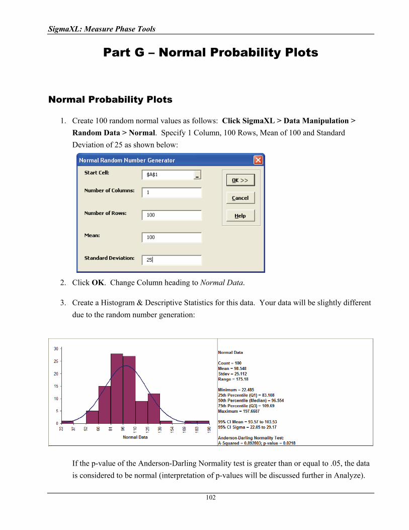
SigmaXL: Measure Phase Tools
Part G – Normal Probability Plots
Normal Probability Plots
1. Create 100 random normal values as follows: Click SigmaXL > Data Manipulation >
Random Data > Normal. Specify 1 Column, 100 Rows, Mean of 100 and Standard
Deviation of 25 as shown below:
2. Click OK. Change Column heading to Normal Data.
3. Create a Histogram & Descriptive Statistics for this data. Your data will be slightly different
due to the random number generation:
If the p-value of the Anderson-Darling Normality test is greater than or equal to .05, the data
is considered to be normal (interpretation of p-values will be discussed further in Analyze).
102
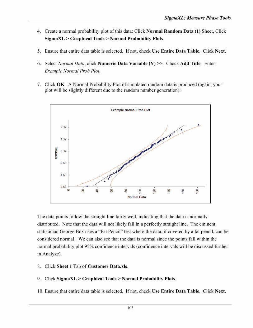
SigmaXL: Measure Phase Tools
4. Create a normal probability plot of this data: Click Normal Random Data (1) Sheet, Click
SigmaXL > Graphical Tools > Normal Probability Plots.
5. Ensure that entire data table is selected. If not, check Use Entire Data Table. Click Next.
6. Select Normal Data, click Numeric Data Variable (Y) >>. Check Add Title. Enter
Example Normal Prob Plot.
7. Click OK. A Normal Probability Plot of simulated random data is produced (again, your
plot will be slightly different due to the random number generation):
The data points follow the straight line fairly well, indicating that the data is normally
distributed. Note that the data will not likely fall in a perfectly straight line. The eminent
statistician George Box uses a “Fat Pencil” test where the data, if covered by a fat pencil, can be
considered normal! We can also see that the data is normal since the points fall within the
normal probability plot 95% confidence intervals (confidence intervals will be discussed further
in Analyze).
8. Click Sheet 1 Tab of Customer Data.xls.
9. Click SigmaXL > Graphical Tools > Normal Probability Plots.
10. Ensure that entire data table is selected. If not, check Use Entire Data Table. Click Next.
103
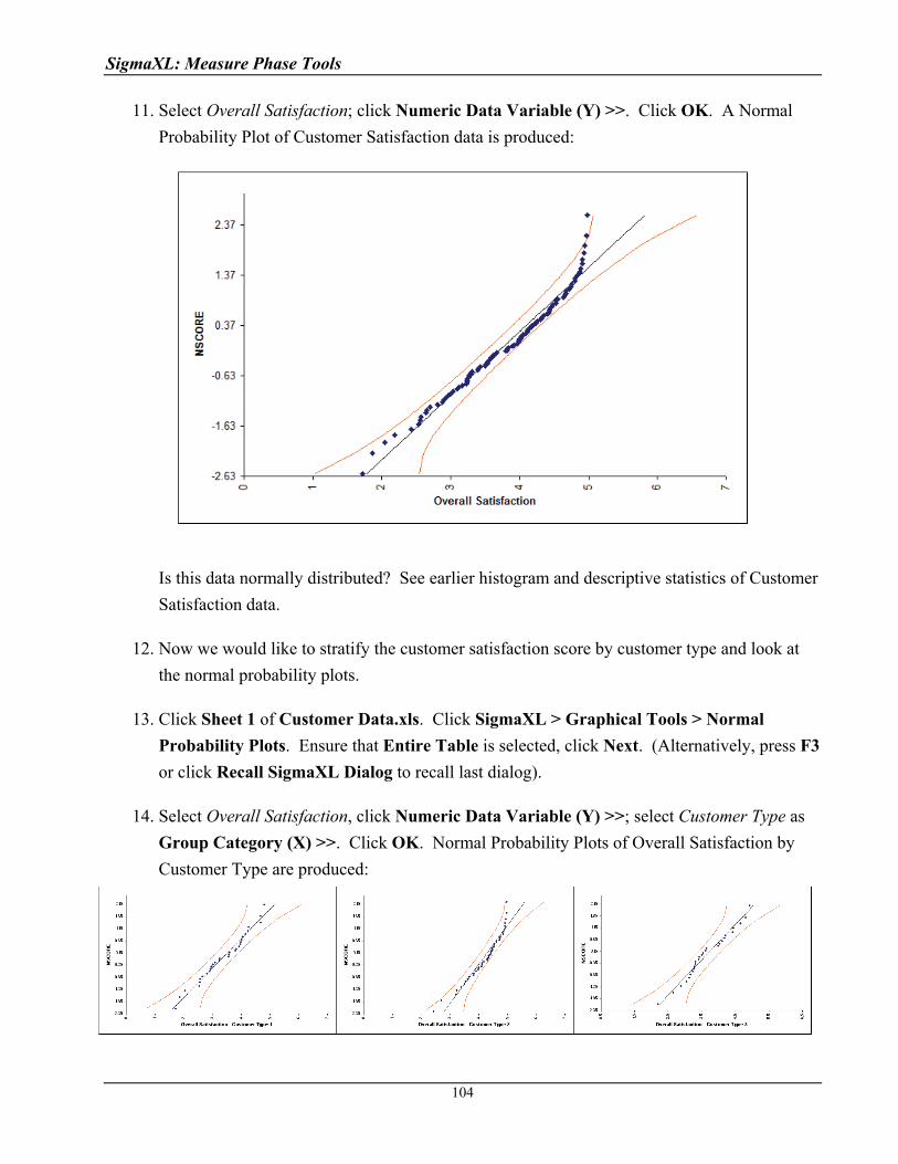
SigmaXL: Measure Phase Tools
11. Select Overall Satisfaction; click Numeric Data Variable (Y) >>. Click OK. A Normal
Probability Plot of Customer Satisfaction data is produced:
Is this data normally distributed? See earlier histogram and descriptive statistics of Customer
Satisfaction data.
12. Now we would like to stratify the customer satisfaction score by customer type and look at
the normal probability plots.
13. Click Sheet 1 of Customer Data.xls. Click SigmaXL > Graphical Tools > Normal
Probability Plots. Ensure that Entire Table is selected, click Next. (Alternatively, press F3
or click Recall SigmaXL Dialog to recall last dialog).
14. Select Overall Satisfaction, click Numeric Data Variable (Y) >>; select Customer Type as
Group Category (X) >>. Click OK. Normal Probability Plots of Overall Satisfaction by
Customer Type are produced:
104

SigmaXL: Measure Phase Tools
105
Reviewing these normal probability plots, along with the previously created histograms and descriptive statistics, we see that the satisfaction data for customer type 2 is not normal, and skewed left, which is desirable for satisfaction data! Note that although the customer type 2 data falls within the 95% confidence intervals, the Anderson Darling test from descriptive statistics shows p < .05 indicating non-normal data. Smaller sample sizes tend to result in wider confidence intervals, but we still see that the curvature for customer type 2 is quite strong. Tip: Use the Normal Probability Plot (NPP) to distinguish reasons for nonnormality. If the data fails the Anderson Darling (AD) test (with p < 0.05) and forms a curve on the NPP, it is inherently nonnormal or skewed. Calculations such as Sigma Level, Pp, Cp, Ppk, Cpk assume normality and will therefore be affected. Consider transforming the data using LN(Y) or SQRT(Y) or using the Box-Cox Transformation tool (SigmaXL > Data Manipulation > Box-Cox Transformation) to make the data normal. Of course, whatever transformation you apply to your data, you must also apply to your specification limits. See also the Process Capability for nonnormal data tools. If the data fails the AD normality test, but the bulk of the data forms a straight line and there are some outliers, the outliers are driving the nonnormality. Do not attempt to transform this data! Determine the root cause for the outliers and take corrective action on those root causes.
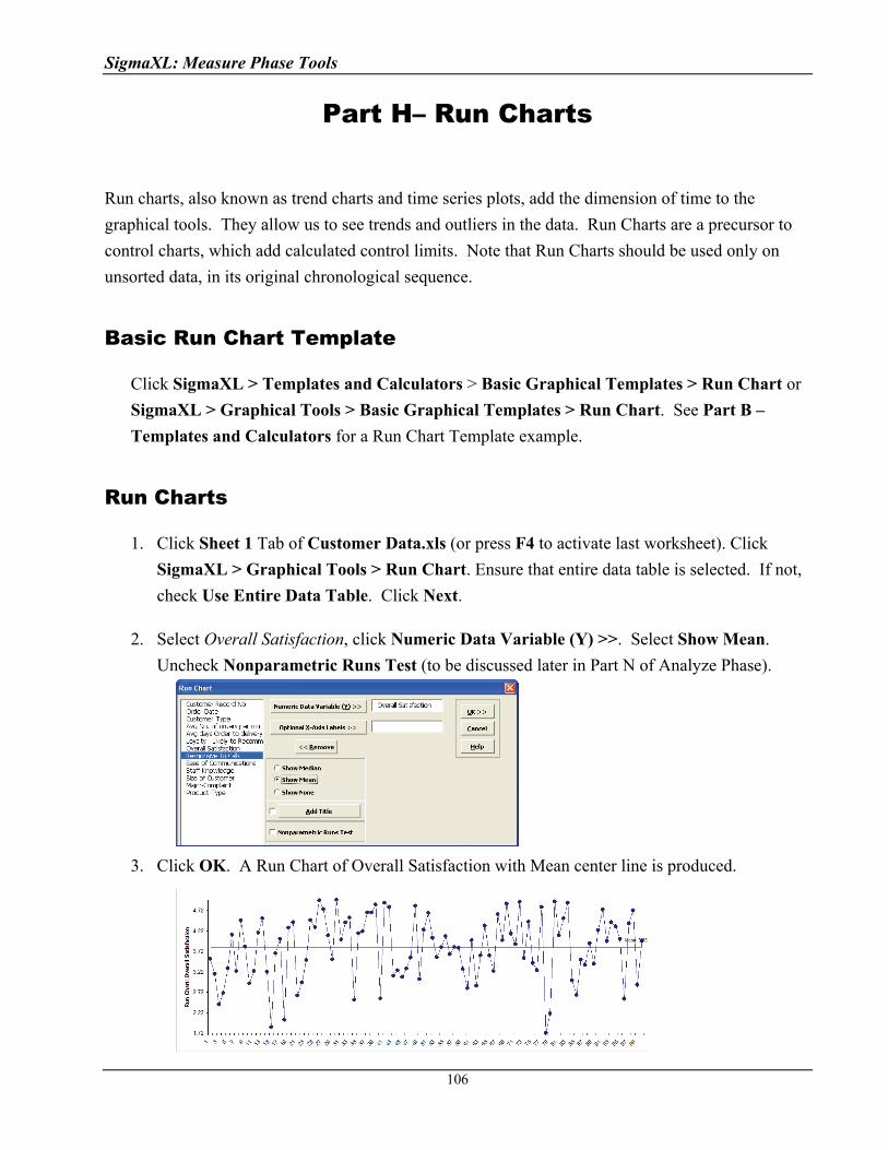
SigmaXL: Measure Phase Tools
Part H– Run Charts
Run charts, also known as trend charts and time series plots, add the dimension of time to the
graphical tools. They allow us to see trends and outliers in the data. Run Charts are a precursor to
control charts, which add calculated control limits. Note that Run Charts should be used only on
unsorted data, in its original chronological sequence.
Basic Run Chart Template
Click SigmaXL > Templates and Calculators > Basic Graphical Templates > Run Chart or
SigmaXL > Graphical Tools > Basic Graphical Templates > Run Chart. See Part B –
Templates and Calculators for a Run Chart Template example.
Run Charts
1. Click Sheet 1 Tab of Customer Data.xls (or press F4 to activate last worksheet). Click
SigmaXL > Graphical Tools > Run Chart. Ensure that entire data table is selected. If not,
check Use Entire Data Table. Click Next.
2. Select Overall Satisfaction, click Numeric Data Variable (Y) >>. Select Show Mean.
Uncheck Nonparametric Runs Test (to be discussed later in Part N of Analyze Phase).
3. Click OK. A Run Chart of Overall Satisfaction with Mean center line is produced.
106
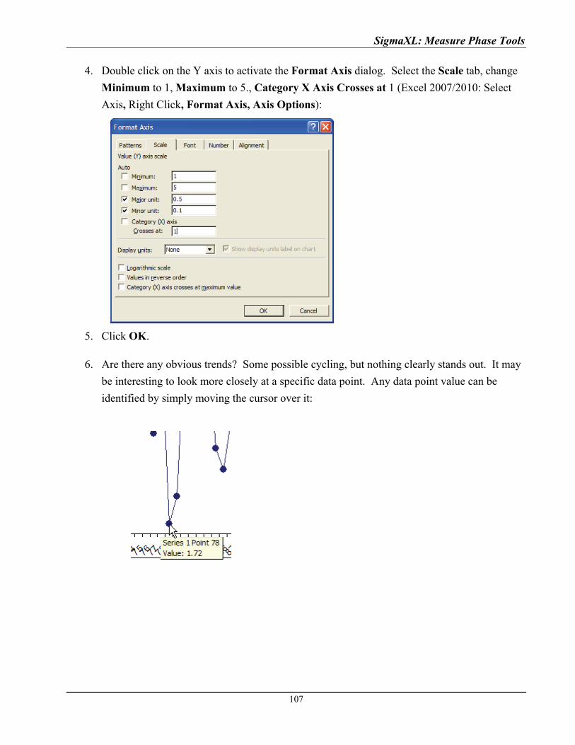
SigmaXL: Measure Phase Tools
4. Double click on the Y axis to activate the Format Axis dialog. Select the Scale tab, change
Minimum to 1, Maximum to 5., Category X Axis Crosses at 1 (Excel 2007/2010: Select
Axis, Right Click, Format Axis, Axis Options):
5. Click OK.
6. Are there any obvious trends? Some possible cycling, but nothing clearly stands out. It may
be interesting to look more closely at a specific data point. Any data point value can be
identified by simply moving the cursor over it:
107
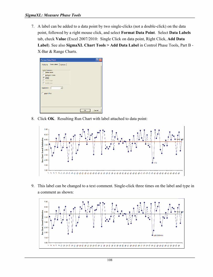
SigmaXL: Measure Phase Tools
7. A label can be added to a data point by two single-clicks (not a double-click) on the data
point, followed by a right mouse click, and select Format Data Point. Select Data Labels
tab, check Value (Excel 2007/2010: Single Click on data point, Right Click, Add Data
Label). See also SigmaXL Chart Tools > Add Data Label in Control Phase Tools, Part B -
X-Bar & Range Charts.
8. Click OK. Resulting Run Chart with label attached to data point:
9. This label can be changed to a text comment. Single-click three times on the label and type in
a comment as shown:
108
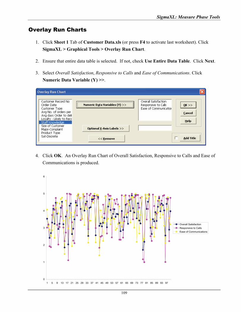
SigmaXL: Measure Phase Tools
Overlay Run Charts
1. Click Sheet 1 Tab of Customer Data.xls (or press F4 to activate last worksheet). Click
SigmaXL > Graphical Tools > Overlay Run Chart.
2. Ensure that entire data table is selected. If not, check Use Entire Data Table. Click Next.
3. Select Overall Satisfaction, Responsive to Calls and Ease of Communications. Click
Numeric Data Variable (Y) >>.
4. Click OK. An Overlay Run Chart of Overall Satisfaction, Responsive to Calls and Ease of
Communications is produced.
0
1
2
3
4
5
6
1 5 9 13 17 21 25 29 33 37 41 45 49 53 57 61 65 69 73 77 81 85 89 93 97
Overall Satisfaction
Responsive to Calls
Ease of Communications
109
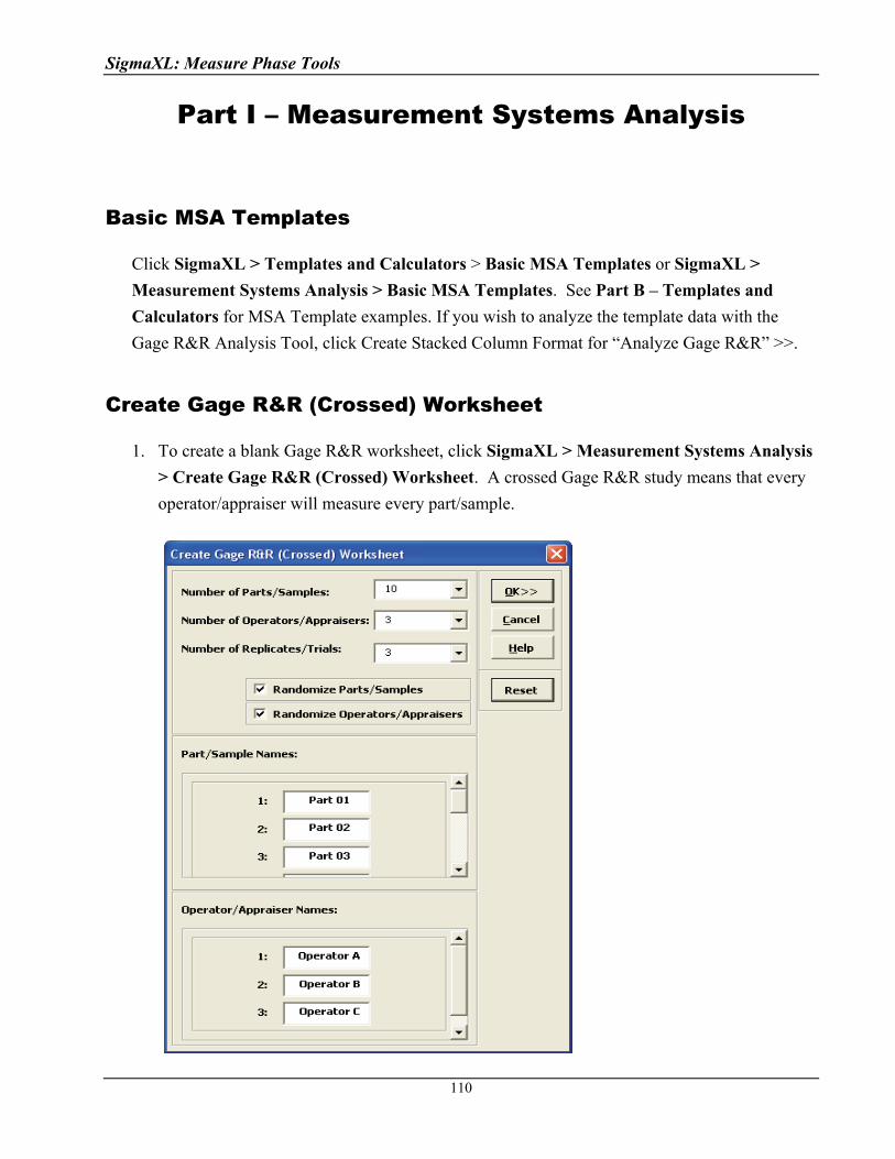
SigmaXL: Measure Phase Tools
Part I – Measurement Systems Analysis
Basic MSA Templates
Click SigmaXL > Templates and Calculators > Basic MSA Templates or SigmaXL >
Measurement Systems Analysis > Basic MSA Templates. See Part B – Templates and
Calculators for MSA Template examples. If you wish to analyze the template data with the
Gage R&R Analysis Tool, click Create Stacked Column Format for “Analyze Gage R&R” >>.
Create Gage R&R (Crossed) Worksheet
1. To create a blank Gage R&R worksheet, click SigmaXL > Measurement Systems Analysis
> Create Gage R&R (Crossed) Worksheet. A crossed Gage R&R study means that every
operator/appraiser will measure every part/sample.
110

SigmaXL: Measure Phase Tools
2. The default settings are 10 Parts, 3 Operators, 3 Replicates with Parts and Operators
randomized. Clicking the Reset button will restore the dialog to these default settings.
3. Part and Operator names can be edited.
4. Click OK. The following worksheet is produced:
5. Your worksheet order will be different due to the randomization. The results of the Gage
R&R study are entered in the yellow highlighted Measurement cells.
Analyze Gage R&R (Crossed)
1. Open the file Gage RR – AIAG.xls. This is an example from the Automotive Industry
Action Group (AIAG) MSA Reference Manual, 3rd Edition, page 101. Note that parts were
measured in random order, but the worksheet is given in standard order.
2. Click SigmaXL > Measurement Systems Analysis > Analyze Gage R&R (Crossed). The
data worksheet is recognized by SigmaXL and highlighted automatically. Click Next.
111
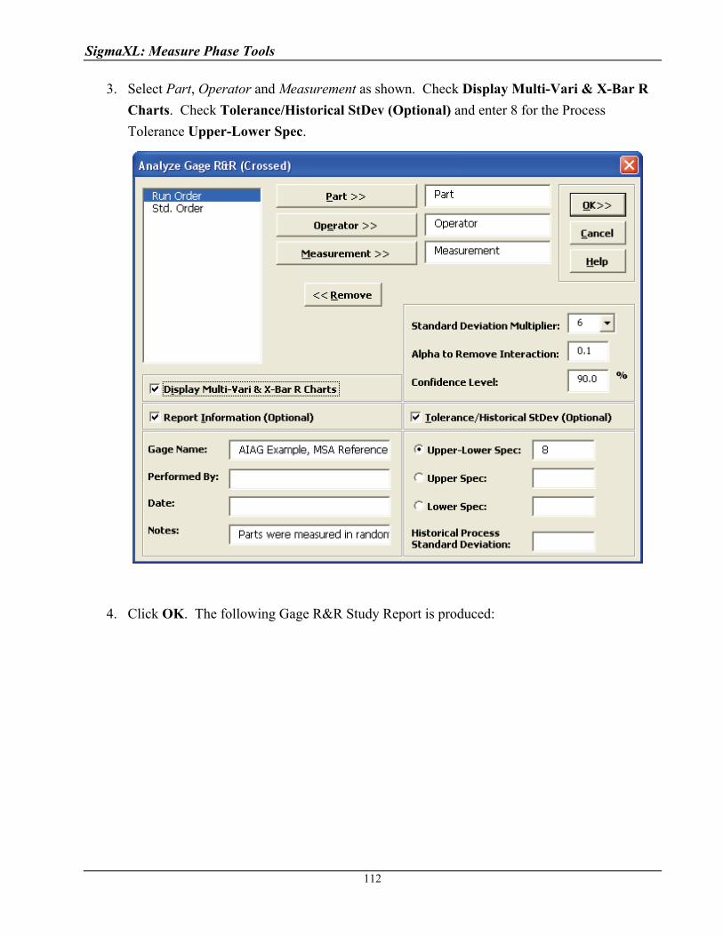
SigmaXL: Measure Phase Tools
3. Select Part, Operator and Measurement as shown. Check Display Multi-Vari & X-Bar R
Charts. Check Tolerance/Historical StDev (Optional) and enter 8 for the Process
Tolerance Upper-Lower Spec.
4. Click OK. The following Gage R&R Study Report is produced:
112

SigmaXL: Measure Phase Tools SigmaXL: Measure Phase Tools
113 113

SigmaXL: Measure Phase Tools
5. The first ANOVA table shows that the Operator * Part Interaction is not significant with the
P-value = 0.9741 (greater than the alpha-to-remove value of 0.1). The second ANOVA table
shows the results excluding the Part * Operator Interaction.
6. The cells shaded in light blue highlight the critical metrics: Gage R&R % Total Variation
(also known as %R&R) and %Tolerance: < 10% indicates a good measurement system;
> 30% indicates an unacceptable measurement system. The Number of Distinct Categories
should be at least 5. Initial analysis shows that this is a marginal measurement system.
(Traditionally NDC is truncated to an integer value, but SigmaXL reports a more informative
one decimal place).
7. SigmaXL also reports the confidence intervals for the Gage R&R metrics. Note that when
the confidence intervals are taken into account, it is possible that this measurement system is
totally inadequate. This strongly suggests that the measurement system needs to be improved
but it also points out the weakness of the traditional Gage R&R study with 10 Parts, 3
Operators, and 3 Replicates. These sample sizes will typically yield wide confidence
intervals. For statistical details of the Gage R&R confidence intervals see Burdick, R. K.,
Borror, C. M., and Montgomery, D. C., “Design and Analysis of Gauge R&R Studies:
Making Decisions with Confidence Intervals in Random and Mixed ANOVA Models”,
ASA-SIAM Series on Statistics and Applied Probability, 2005.
8. Click on the Gage R&R – Multi-Vari Sheet tab to view the Multi-Vari Chart:
The Multi-Vari chart shows each Part as a separate graph. Each Operator’s response
readings are denoted as a vertical line with the top tick corresponding to the Maximum value,
bottom tick is the Minimum, and the middle tick is the Mean. The horizontal line across
each graph is the overall average for each part.
114
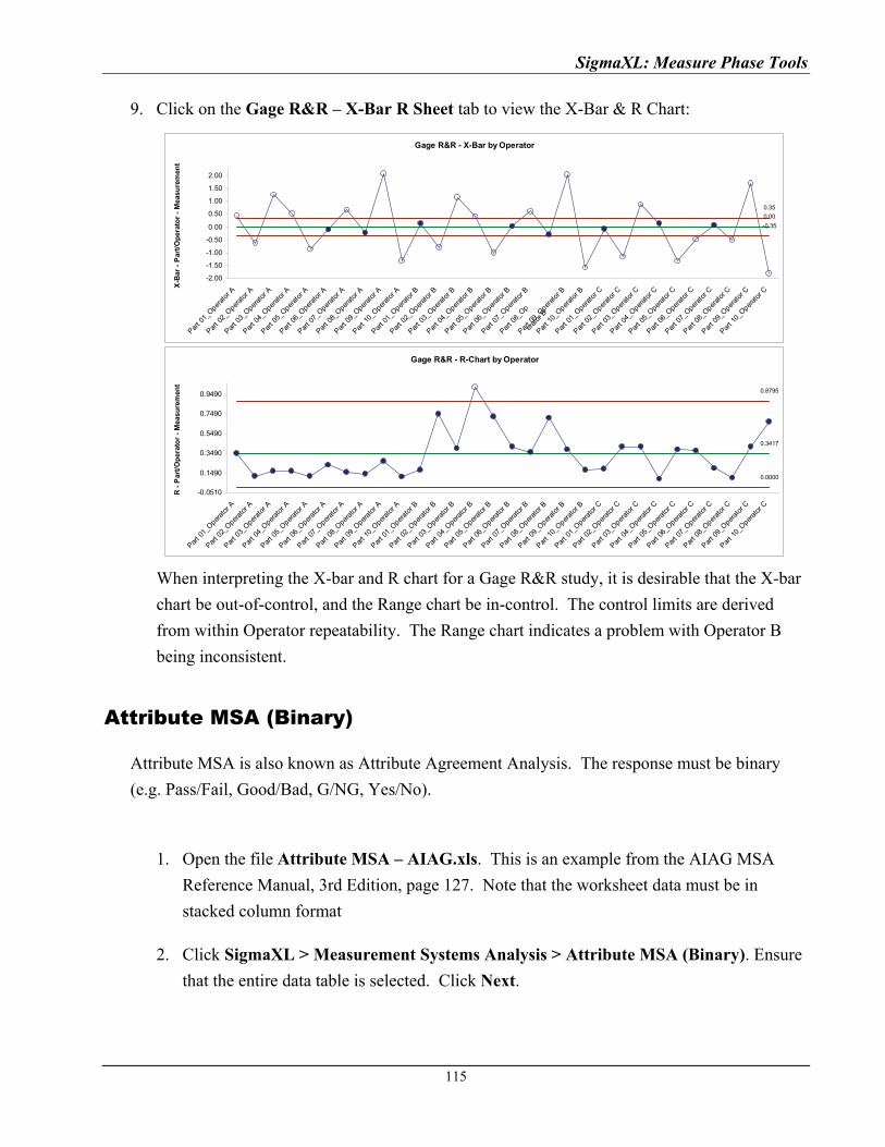
SigmaXL: Measure Phase Tools
9. Click on the Gage R&R – X-Bar R Sheet tab to view the X-Bar & R Chart:
When interpreting the X-bar and R chart for a Gage R&R study, it is desirable that the X-bar
chart be out-of-control, and the Range chart be in-control. The control limits are derived
from within Operator repeatability. The Range chart indicates a problem with Operator B
being inconsistent.
Gage R&R - X-Bar by Operator
0.00
-0.35
0.35
-2.00
-1.50
-1.00
-0.50
0.00
0.50
1.00
1.50
2.00
Part 0
1_Oper
ator
A
Part 0
2_Oper
ator
A
Part 0
3_Oper
ator
A
Part 0
4_Oper
ator
A
Part 0
5_Oper
ator
A
Part 0
6_Oper
ator
A
Part 0
7_Oper
ator
A
Part 0
8_Oper
ator
A
Part 0
9_Oper
ator
A
Part 1
0_Oper
ator
A
Part 0
1_Oper
ator
B
Part 0
2_Oper
ator
B
Part 0
3_Oper
ator
B
Part 0
4_Oper
ator
B
Part 0
5_Oper
ator
B
Part 0
6_Oper
ator
B
Part 0
7_Oper
ator
B
Part 0
8_Oper
ator
B
Part 0
9_Oper
ator
B
Part 1
0_Oper
ator
B
Part 0
1_Oper
ator
C
Part 0
2_Oper
ator
C
Part 0
3_Oper
ator
C
Part 0
4_Oper
ator
C
Part 0
5_Oper
ator
C
Part 0
6_Oper
ator
C
Part 0
7_Oper
ator
C
Part 0
8_Oper
ator
C
Part 0
9_Oper
ator
C
Part 1
0_Oper
ator
C
X-B
ar -
Par
t/O
per
ato
r -
Mea
sure
men
t
Gage R&R - R-Chart by Operator
0.3417
0.0000
0.8795
-0.0510
0.1490
0.3490
0.5490
0.7490
0.9490
Part 0
1_Oper
ator
A
Part 0
2_Oper
ator
A
Part 0
3_Oper
ator
A
Part 0
4_Oper
ator
A
Part 0
5_Oper
ator
A
Part 0
6_Oper
ator
A
Part 0
7_Oper
ator
A
Part 0
8_Oper
ator
A
Part 0
9_Oper
ator
A
Part 1
0_Oper
ator
A
Part 0
1_Oper
ator
B
Part 0
2_Oper
ator
B
Part 0
3_Oper
ator
B
Part 0
4_Oper
ator
B
Part 0
5_Oper
ator
B
Part 0
6_Oper
ator
B
Part 0
7_Oper
ator
B
Part 0
8_Oper
ator
B
Part 0
9_Oper
ator
B
Part 1
0_Oper
ator
B
Part 0
1_Oper
ator
C
Part 0
2_Oper
ator
C
Part 0
3_Oper
ator
C
Part 0
4_Oper
ator
C
Part 0
5_Oper
ator
C
Part 0
6_Oper
ator
C
Part 0
7_Oper
ator
C
Part 0
8_Oper
ator
C
Part 0
9_Oper
ator
C
Part 1
0_Oper
ator
C
R -
Par
t/O
per
ato
r -
Mea
sure
men
t
Attribute MSA (Binary)
Attribute MSA is also known as Attribute Agreement Analysis. The response must be binary
(e.g. Pass/Fail, Good/Bad, G/NG, Yes/No).
1. Open the file Attribute MSA – AIAG.xls. This is an example from the AIAG MSA
Reference Manual, 3rd Edition, page 127. Note that the worksheet data must be in
stacked column format
2. Click SigmaXL > Measurement Systems Analysis > Attribute MSA (Binary). Ensure
that the entire data table is selected. Click Next.
115
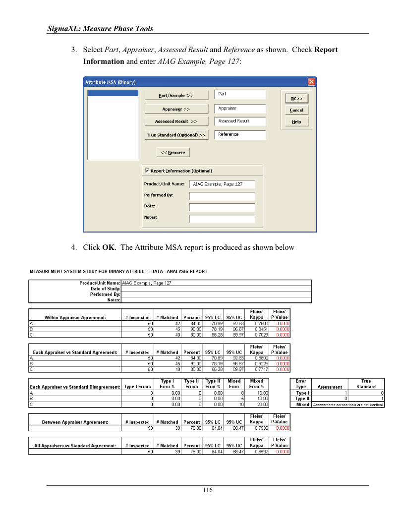
SigmaXL: Measure Phase Tools
3. Select Part, Appraiser, Assessed Result and Reference as shown. Check Report
Information and enter AIAG Example, Page 127:
4. Click OK. The Attribute MSA report is produced as shown below
:
116
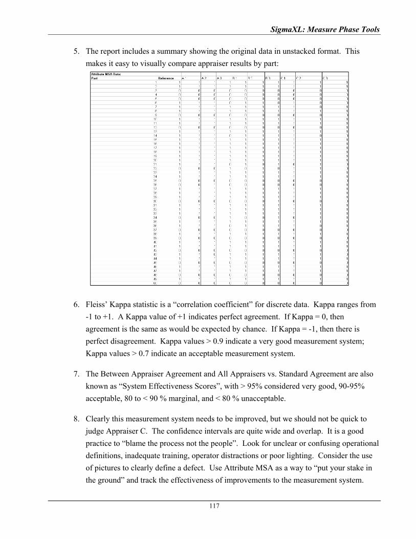
SigmaXL: Measure Phase Tools
5. The report includes a summary showing the original data in unstacked format. This
makes it easy to visually compare appraiser results by part:
6. Fleiss’ Kappa statistic is a “correlation coefficient” for discrete data. Kappa ranges from
-1 to +1. A Kappa value of +1 indicates perfect agreement. If Kappa = 0, then
agreement is the same as would be expected by chance. If Kappa = -1, then there is
perfect disagreement. Kappa values > 0.9 indicate a very good measurement system;
Kappa values > 0.7 indicate an acceptable measurement system.
7. The Between Appraiser Agreement and All Appraisers vs. Standard Agreement are also
known as “System Effectiveness Scores”, with > 95% considered very good, 90-95%
acceptable, 80 to < 90 % marginal, and < 80 % unacceptable.
8. Clearly this measurement system needs to be improved, but we should not be quick to
judge Appraiser C. The confidence intervals are quite wide and overlap. It is a good
practice to “blame the process not the people”. Look for unclear or confusing operational
definitions, inadequate training, operator distractions or poor lighting. Consider the use
of pictures to clearly define a defect. Use Attribute MSA as a way to “put your stake in
the ground” and track the effectiveness of improvements to the measurement system.
117
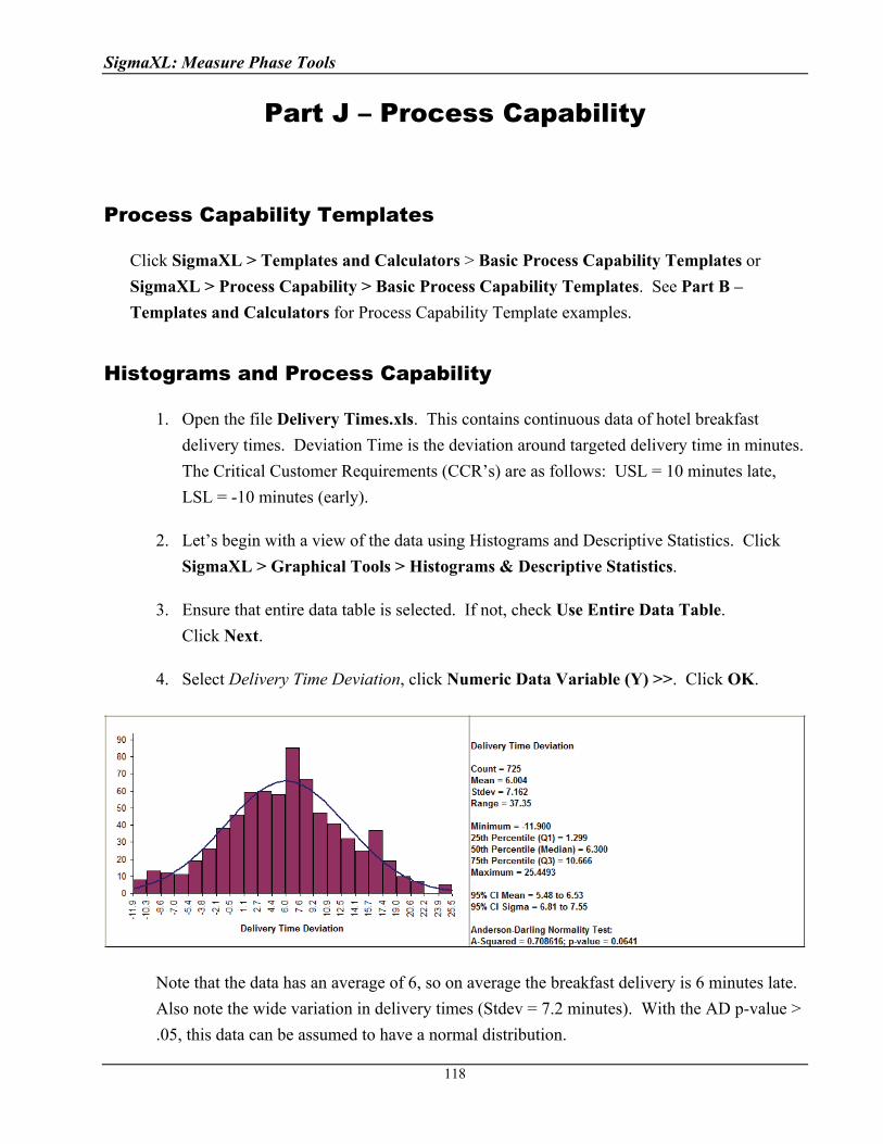
SigmaXL: Measure Phase Tools
Part J – Process Capability
Process Capability Templates
Click SigmaXL > Templates and Calculators > Basic Process Capability Templates or
SigmaXL > Process Capability > Basic Process Capability Templates. See Part B –
Templates and Calculators for Process Capability Template examples.
Histograms and Process Capability
1. Open the file Delivery Times.xls. This contains continuous data of hotel breakfast
delivery times. Deviation Time is the deviation around targeted delivery time in minutes.
The Critical Customer Requirements (CCR’s) are as follows: USL = 10 minutes late,
LSL = -10 minutes (early).
2. Let’s begin with a view of the data using Histograms and Descriptive Statistics. Click
SigmaXL > Graphical Tools > Histograms & Descriptive Statistics.
3. Ensure that entire data table is selected. If not, check Use Entire Data Table.
Click Next.
4. Select Delivery Time Deviation, click Numeric Data Variable (Y) >>. Click OK.
Note that the data has an average of 6, so on average the breakfast delivery is 6 minutes late.
Also note the wide variation in delivery times (Stdev = 7.2 minutes). With the AD p-value >
.05, this data can be assumed to have a normal distribution.
118
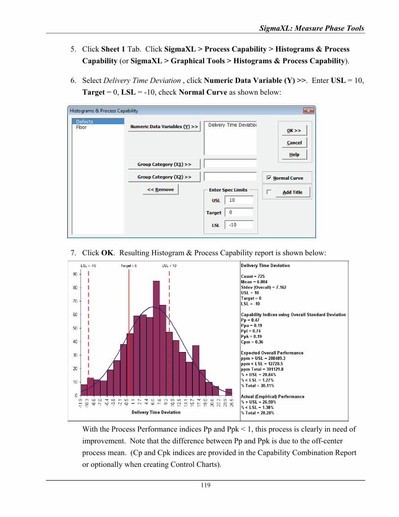
SigmaXL: Measure Phase Tools
5. Click Sheet 1 Tab. Click SigmaXL > Process Capability > Histograms & Process
Capability (or SigmaXL > Graphical Tools > Histograms & Process Capability).
6. Select Delivery Time Deviation , click Numeric Data Variable (Y) >>. Enter USL = 10,
Target = 0, LSL = -10, check Normal Curve as shown below:
7. Click OK. Resulting Histogram & Process Capability report is shown below:
With the Process Performance indices Pp and Ppk < 1, this process is clearly in need of
improvement. Note that the difference between Pp and Ppk is due to the off-center
process mean. (Cp and Cpk indices are provided in the Capability Combination Report
or optionally when creating Control Charts).
119
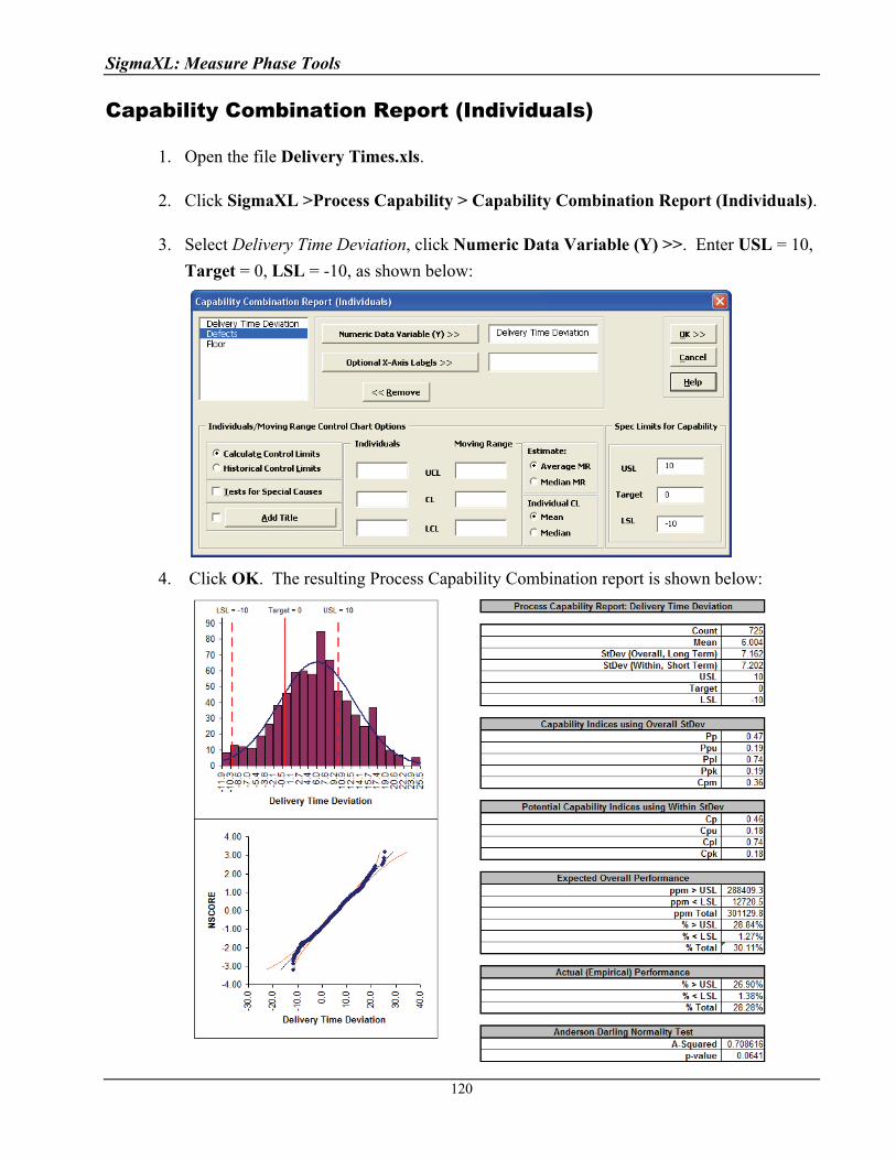
SigmaXL: Measure Phase Tools
Capability Combination Report (Individuals)
1. Open the file Delivery Times.xls.
2. Click SigmaXL >Process Capability > Capability Combination Report (Individuals).
3. Select Delivery Time Deviation, click Numeric Data Variable (Y) >>. Enter USL = 10,
Target = 0, LSL = -10, as shown below:
4. Click OK. The resulting Process Capability Combination report is shown below:
120
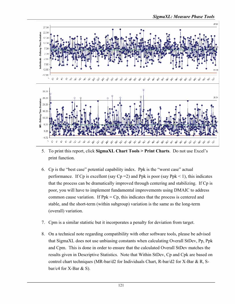
SigmaXL: Measure Phase Tools
5. To print this report, click SigmaXL Chart Tools > Print Charts. Do not use Excel’s
print function.
6. Cp is the “best case” potential capability index. Ppk is the “worst case” actual
performance. If Cp is excellent (say Cp =2) and Ppk is poor (say Ppk < 1), this indicates
that the process can be dramatically improved through centering and stabilizing. If Cp is
poor, you will have to implement fundamental improvements using DMAIC to address
common cause variation. If Ppk = Cp, this indicates that the process is centered and
stable, and the short-term (within subgroup) variation is the same as the long-term
(overall) variation.
7. Cpm is a similar statistic but it incorporates a penalty for deviation from target.
8. On a technical note regarding compatibility with other software tools, please be advised
that SigmaXL does not use unbiasing constants when calculating Overall StDev, Pp, Ppk
and Cpm. This is done in order to ensure that the calculated Overall StDev matches the
results given in Descriptive Statistics. Note that Within StDev, Cp and Cpk are based on
control chart techniques (MR-bar/d2 for Individuals Chart, R-bar/d2 for X-Bar & R, S-
bar/c4 for X-Bar & S).
121
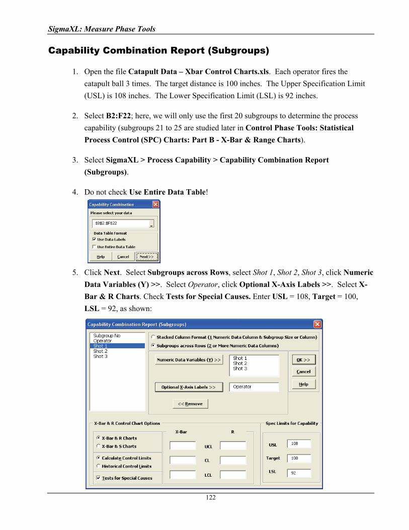
SigmaXL: Measure Phase Tools
Capability Combination Report (Subgroups)
1. Open the file Catapult Data – Xbar Control Charts.xls. Each operator fires the
catapult ball 3 times. The target distance is 100 inches. The Upper Specification Limit
(USL) is 108 inches. The Lower Specification Limit (LSL) is 92 inches.
2. Select B2:F22; here, we will only use the first 20 subgroups to determine the process
capability (subgroups 21 to 25 are studied later in Control Phase Tools: Statistical
Process Control (SPC) Charts: Part B - X-Bar & Range Charts).
3. Select SigmaXL > Process Capability > Capability Combination Report
(Subgroups).
4. Do not check Use Entire Data Table!
5. Click Next. Select Subgroups across Rows, select Shot 1, Shot 2, Shot 3, click Numeric
Data Variables (Y) >>. Select Operator, click Optional X-Axis Labels >>. Select X-
Bar & R Charts. Check Tests for Special Causes. Enter USL = 108, Target = 100,
LSL = 92, as shown:
122

SigmaXL: Measure Phase Tools
6. Click OK. The resulting Process Capability Combination report is shown below:
123
SigmaXL: Measure Phase Tools
124
Capability Combination Report (Individuals Nonnormal) An important assumption for process capability analysis is that the data be normally distributed. The Capability Combination Report (Individuals Nonnormal) allows you to transform the data to normality or utilize nonnormal distributions, including:
o Box-Cox Transformation (includes an automatic threshold option so that data with negative values can be transformed)
o Johnson Transformation o Distributions supported:
Half-Normal Lognormal (2 & 3 parameter) Exponential (1 & 2 parameter) Weibull (2 & 3 parameter) Beta (2 & 4 parameter) Gamma (2 & 3 parameter) Logistic Loglogistic (2 & 3 parameter) Largest Extreme Value Smallest Extreme Value
o Automatic Best Fit based on AD p-value For technical details, see Appendix: Statistical Details for Nonnormal Distributions and Transformations. Also see Andrew Sleeper, Six Sigma Distribution Modeling, for further information on these methods. Note that these transformations and distributions are particularly effective for inherently skewed data but should not be used with bimodal data or where the nonnormality is due to outliers (typically identified with a Normal Probability Plot). In these cases, you should identify the reason for the bimodality or outliers and take corrective action. Another common reason for nonnormal data is poor measurement discrimination leading to “chunky” data. In this case, attempts should be made to improve the measurement system. Box-Cox Transformation SigmaXL’s default setting is to use the Box-Cox transformation which is the most common approach to dealing with nonnormal data. Box-Cox is used to convert nonnormal data to normal by applying a power transformation, Y^lambda, where lambda varies from -5 to +5. You may select rounded or optimal lambda. Rounded is typically preferred since it will result in a more “intuitive” transformation such as Ln(Y) (lambda=0) or SQRT(Y) (lambda=0.5). If the data includes zero or negative values, select Lambda & Threshold. SigmaXL will solve for an optimal threshold which is a shift factor on the data so that all of the values are positive.
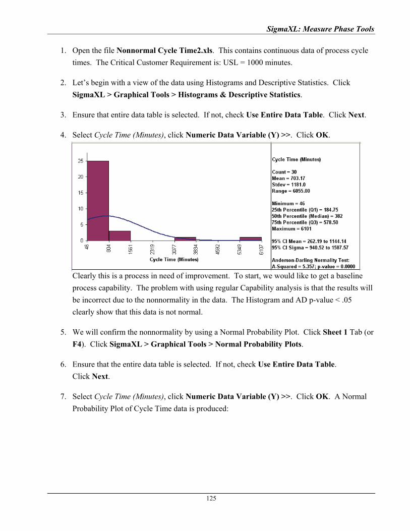
SigmaXL: Measure Phase Tools
1. Open the file Nonnormal Cycle Time2.xls. This contains continuous data of process cycle
times. The Critical Customer Requirement is: USL = 1000 minutes.
2. Let’s begin with a view of the data using Histograms and Descriptive Statistics. Click
SigmaXL > Graphical Tools > Histograms & Descriptive Statistics.
3. Ensure that entire data table is selected. If not, check Use Entire Data Table. Click Next.
4. Select Cycle Time (Minutes), click Numeric Data Variable (Y) >>. Click OK.
Clearly this is a process in need of improvement. To start, we would like to get a baseline
process capability. The problem with using regular Capability analysis is that the results will
be incorrect due to the nonnormality in the data. The Histogram and AD p-value < .05
clearly show that this data is not normal.
5. We will confirm the nonnormality by using a Normal Probability Plot. Click Sheet 1 Tab (or
F4). Click SigmaXL > Graphical Tools > Normal Probability Plots.
6. Ensure that the entire data table is selected. If not, check Use Entire Data Table.
Click Next.
7. Select Cycle Time (Minutes), click Numeric Data Variable (Y) >>. Click OK. A Normal
Probability Plot of Cycle Time data is produced:
125

SigmaXL: Measure Phase Tools
-2.17
-1.67
-1.17
-0.67
-0.17
0.33
0.83
1.33
1.83
2.33
-400
0
-200
0 0
2000
4000
6000
8000
Cycle Time (Minutes)
NS
CO
RE
8. The curvature in this normal probability plot confirms that this data is not normal.
9. For now, let us ignore the nonnormal issue and perform a Process Capability study assuming
a normal distribution. Click Sheet 1 Tab. Click SigmaXL > Process Capability >
Capability Combination Report (Individuals).
10. Select Cycle Time (Minutes), click Numeric Data Variable (Y) >>. Enter USL = 1000;
delete previous Target and LSL settings.
11. Click OK. The resulting Process Capability Report is shown below:
126
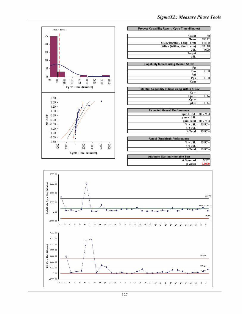
SigmaXL: Measure Phase Tools
127
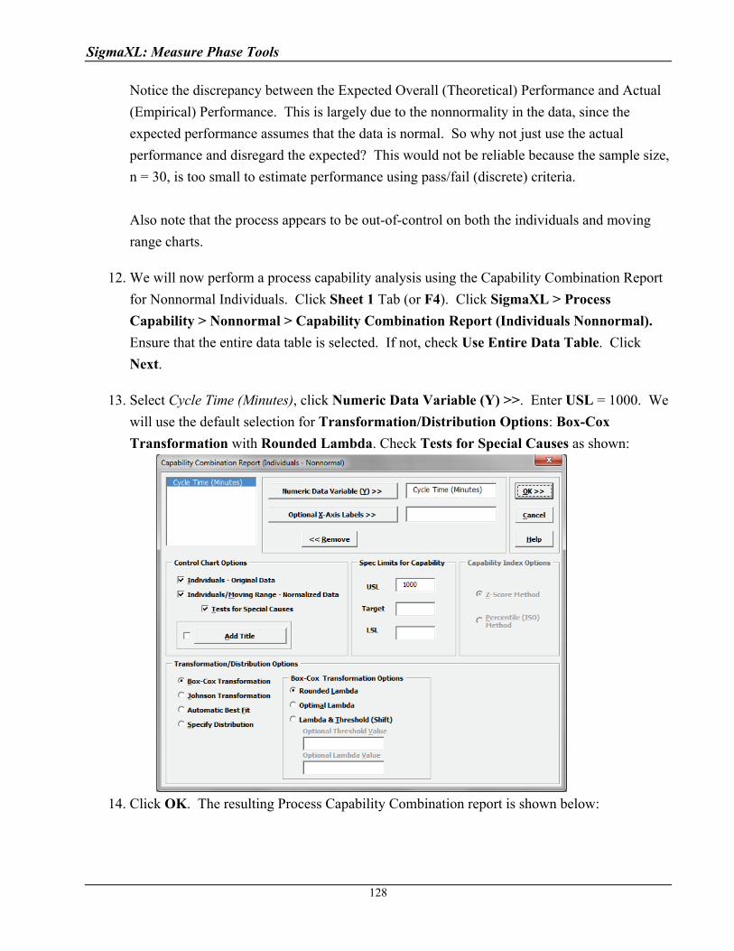
SigmaXL: Measure Phase Tools
Notice the discrepancy between the Expected Overall (Theoretical) Performance and Actual
(Empirical) Performance. This is largely due to the nonnormality in the data, since the
expected performance assumes that the data is normal. So why not just use the actual
performance and disregard the expected? This would not be reliable because the sample size,
n = 30, is too small to estimate performance using pass/fail (discrete) criteria.
Also note that the process appears to be out-of-control on both the individuals and moving
range charts.
12. We will now perform a process capability analysis using the Capability Combination Report
for Nonnormal Individuals. Click Sheet 1 Tab (or F4). Click SigmaXL > Process
Capability > Nonnormal > Capability Combination Report (Individuals Nonnormal).
Ensure that the entire data table is selected. If not, check Use Entire Data Table. Click
Next.
13. Select Cycle Time (Minutes), click Numeric Data Variable (Y) >>. Enter USL = 1000. We
will use the default selection for Transformation/Distribution Options: Box-Cox
Transformation with Rounded Lambda. Check Tests for Special Causes as shown:
14. Click OK. The resulting Process Capability Combination report is shown below:
128
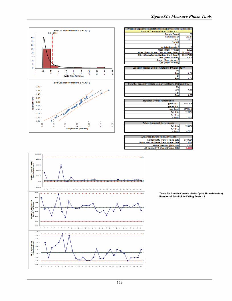
SigmaXL: Measure Phase Tools
129

SigmaXL: Measure Phase Tools
130
The AD Normality P-Value Transformed Data value of 0.404 confirms that the Box-Cox
transformation to normality was successful. The process capability indices and expected
performance can now be used to establish a baseline performance. Note that there are no out-of-
control signals on the control charts, so the signals observed earlier when normality was assumed
were false alarms.
The Individuals – Original Data chart displays the untransformed data with control limits calculated as:
UCL = 99.865 percentile
CL = 50th percentile
LCL = 0.135 percentile
The benefit of displaying this chart is that one can observe the original untransformed data. Since
the control limits are based on percentiles, this represents the overall, long term variation rather than
the typical short term variation. The limits will likely be nonsymmetrical.
The Individuals/Moving Range – Normalized Data chart displays the transformed z-values with
control limits calculated using the standard Shewhart formulas for Individuals and Moving Range
charts. The benefit of using this chart is that tests for special causes can be applied and the control
limits are based on short term variation. The disadvantage is that one is observing transformed data
on the chart rather than the original data.
Automatic Best Fit
Now we will redo the capability analysis using the Automatic Best Fit option.
15. Click Recall SigmaXL Dialog menu or press F3 to recall last dialog. Select Automatic
Best Fit as shown:
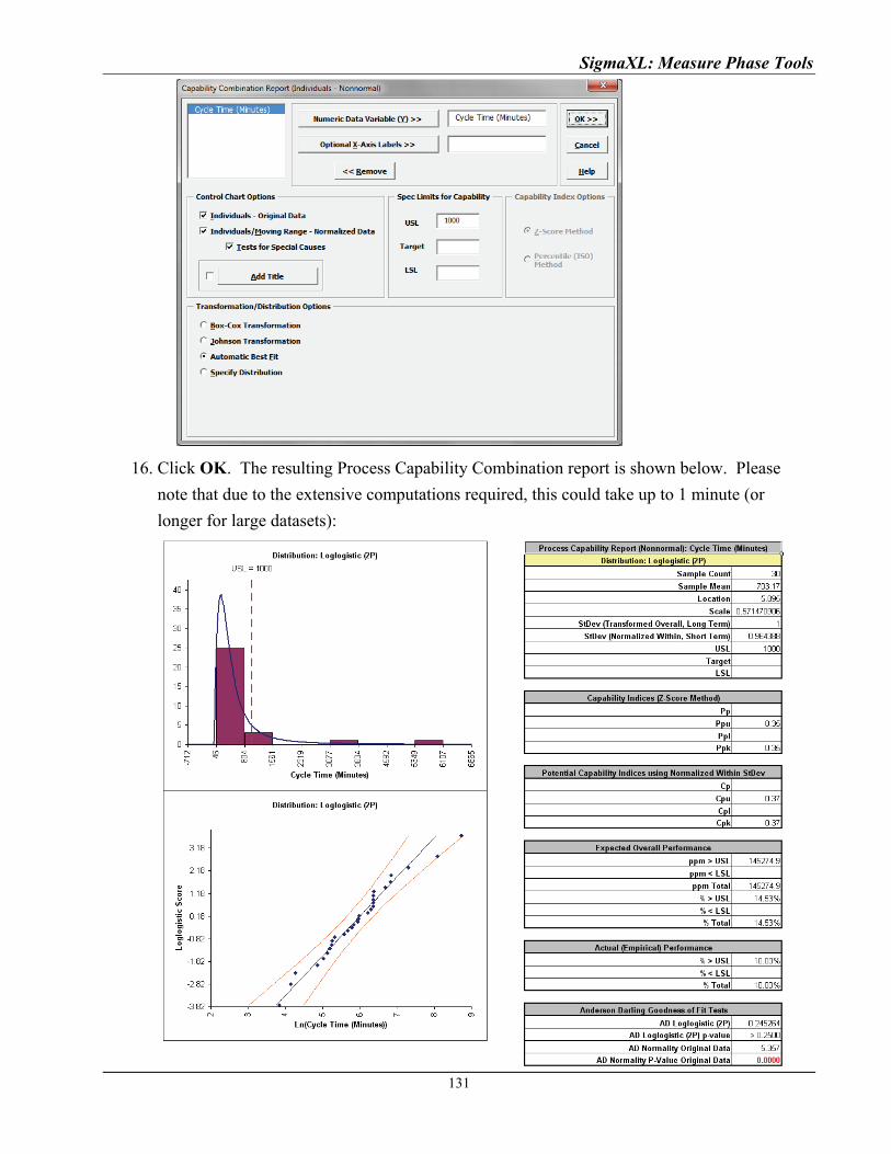
SigmaXL: Measure Phase Tools
16. Click OK. The resulting Process Capability Combination report is shown below. Please
note that due to the extensive computations required, this could take up to 1 minute (or
longer for large datasets):
131
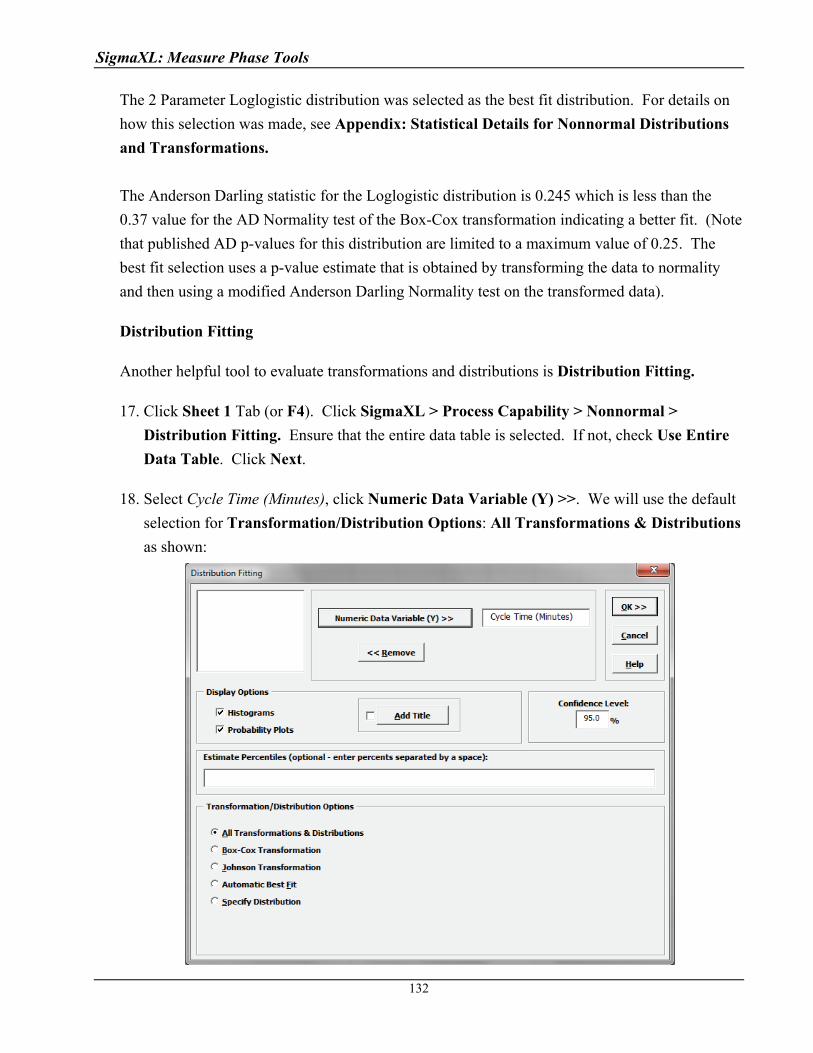
SigmaXL: Measure Phase Tools
The 2 Parameter Loglogistic distribution was selected as the best fit distribution. For details on
how this selection was made, see Appendix: Statistical Details for Nonnormal Distributions
and Transformations.
The Anderson Darling statistic for the Loglogistic distribution is 0.245 which is less than the
0.37 value for the AD Normality test of the Box-Cox transformation indicating a better fit. (Note
that published AD p-values for this distribution are limited to a maximum value of 0.25. The
best fit selection uses a p-value estimate that is obtained by transforming the data to normality
and then using a modified Anderson Darling Normality test on the transformed data).
Distribution Fitting
Another helpful tool to evaluate transformations and distributions is Distribution Fitting.
17. Click Sheet 1 Tab (or F4). Click SigmaXL > Process Capability > Nonnormal >
Distribution Fitting. Ensure that the entire data table is selected. If not, check Use Entire
Data Table. Click Next.
18. Select Cycle Time (Minutes), click Numeric Data Variable (Y) >>. We will use the default
selection for Transformation/Distribution Options: All Transformations & Distributions
as shown:
132
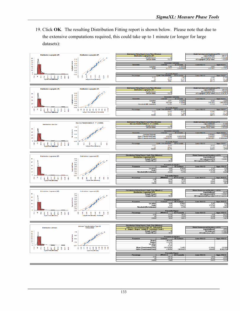
SigmaXL: Measure Phase Tools
19. Click OK. The resulting Distribution Fitting report is shown below. Please note that due to
the extensive computations required, this could take up to 1 minute (or longer for large
datasets):
133
SigmaXL: Measure Phase Tools
134
The distributions and transformations are sorted in descending order using the AD Normality p-
value on the transformed z-score values. Note that the first distribution shown may not be the
selected “best fit”, because the best fit procedure also looks for models that are close but with
fewer parameters.
The reported AD p-values are those derived from the particular distribution. The AD p-value is
not available for distributions with a threshold (except Weibull), so the AD Normality p-value on
the transformed z-score values is used (labeled as Z-Score Est.).
Since the sort order is based on the AD p-values from Z-Score estimates, it is possible that the
reported distribution based AD p-values may not be in perfect descending order. However any
discrepancies based on sort order will likely not be statistically or practically significant.
Some data will have distributions and transformations where the parameters cannot be solved
(e.g., 2-parameter Weibull with negative values). These are excluded from the Distribution
Fitting report.
The parameter estimates and percentile report includes a confidence interval as specified in the
Distribution Fitting dialog, with 95% being the default. Note that the wide intervals here are
due to the small sample size, n = 30.
The control limits for the percentile based Individuals chart will be the 0.135% (lower control
limit), 50% (center line, median) and 99.865% (upper control limit). Additional percentiles may
be entered in the Distribution Fitting dialog.
After reviewing this report, if you wish to perform a process capability analysis with a particular
transformation or distribution, simply select Specify Distribution from the
Transformation/Distribution Options in the Capability Combination Report (Individuals -
Nonnormal) dialog as shown below (using 2 Parameter Loglogistic):

SigmaXL: Measure Phase Tools
135

SigmaXL: Measure Phase Tools
Box-Cox Transformation This is a standalone tool that allows you to visually see how the Box-Cox transformation selects a rounded or optimal lambda value.
1. Open the file Nonnormal Cycle Time2.xls. Select Sheet 1 Tab.
2. Click SigmaXL > Process Capability > Nonnormal > Box-Cox Transformation (or
SigmaXL > Data Manipulation > Box-Cox Transformation or SigmaXL > Control
Charts > Nonnormal > Box-Cox Transformation). Ensure that the entire data table is
selected. If not, check Use Entire Data Table. Click Next.
3. Select Cycle Time (Minutes), click Numeric Data Variable (Y) >>. The selected variable
must contain all positive values.
Tip: Note that while this tool is often successful to transform the data to normality, there
may not be a suitable transformation to make the data normal. The output report indicates
the Anderson-Darling p-value for the transformed data. You may wish to check Do not
store if transformed data is not normal. Another option is Do not store transformed
data if Lambda = 1 falls within 95%CI. This latter option prevents you from using
transformations that do not result in a statistically significant improvement towards
normality.
4. Click OK. The resulting report is shown:
136
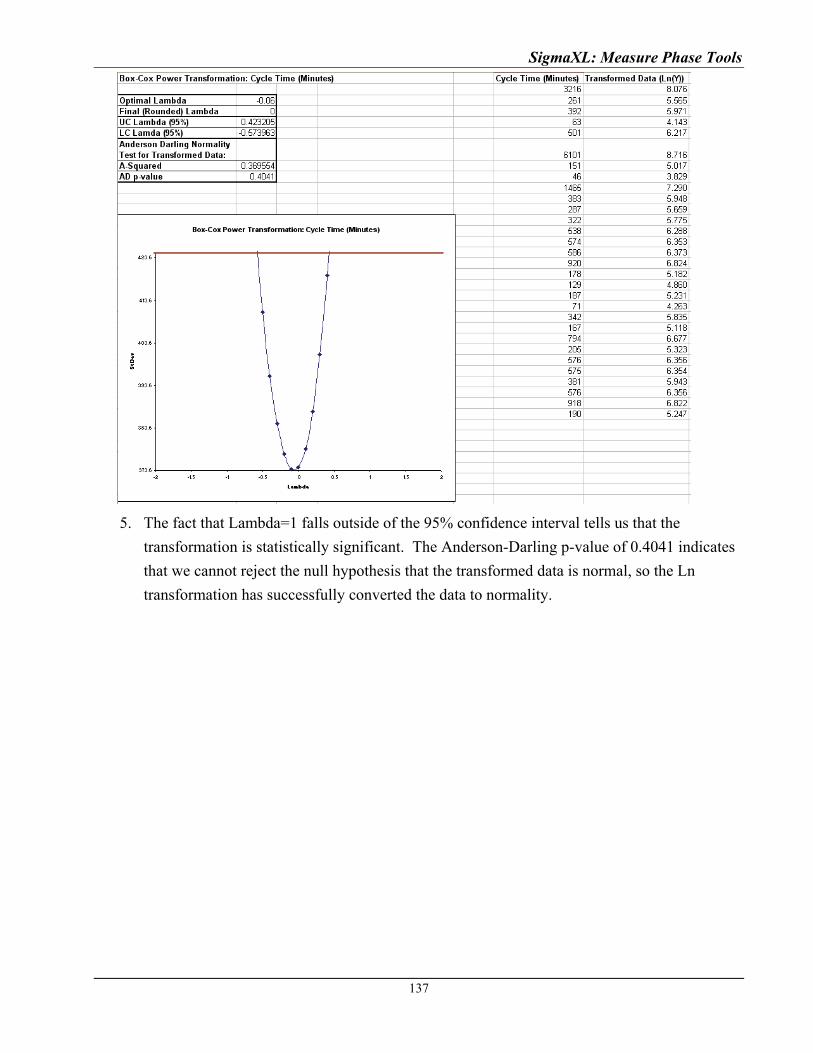
SigmaXL: Measure Phase Tools
5. The fact that Lambda=1 falls outside of the 95% confidence interval tells us that the
transformation is statistically significant. The Anderson-Darling p-value of 0.4041 indicates
that we cannot reject the null hypothesis that the transformed data is normal, so the Ln
transformation has successfully converted the data to normality.
137

SigmaXL: Measure Phase Tools
138
Part K – Reliability/Weibull Analysis
Reliability/Weibull Analysis
The Weibull distribution is a continuous distribution that was publicized by Waloddi Weibull
in 1951. It has become widely used, especially in the reliability field. The Weibull
distribution's popularity resulted from its ability to be used with small sample sizes and its
flexibility. See Dodson, B. “The Weibull Analysis Handbook” Second Edition, ASQ, for
further information. For SigmaXL technical details, see Appendix: Statistical Details for
Nonnormal Distributions and Transformations.
The Weibull distribution can also be used as an alternative to the Box-Cox Transformation to
determine Process Capability Indices or Control Limits for non-normal data.
Weibull is particularly effective when the data are censored, with exact failure times
unknown or suspension of test. Suspension of test is also referred to as right censored.
SigmaXL can analyze complete or right censored data.
1. Open the file Weibull Dodson.xls. This contains right censored time-to-failure data from
Dodson, page 28.
2. Click SigmaXL > Reliability/Weibull Analysis. Ensure that the entire data table is
selected. Click Next.
3. Select Time-to-Fail, click Numeric Response (Y) >>. Note that the selected variable must
contain all positive values. Select Censor Code, click Right Censor Column >>. The
default censor value of 1 will be used. We will use the default method of estimation,
Maximum Likelihood (some reliability practitioners prefer Least Squares Regression (X
on Y) for small sample sizes). Other defaults include Threshold = 0, and Confidence Level
= 90%. Enter time values to estimate survival probabilities as shown:

SigmaXL: Measure Phase Tools
4. The resulting Weibull analysis report is shown:
139
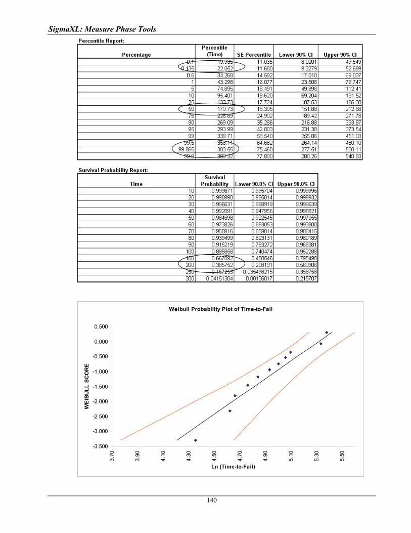
SigmaXL: Measure Phase Tools
Weibull Probability Plot of Time-to-Fail
-3.500
-3.000
-2.500
-2.000
-1.500
-1.000
-0.500
0.000
0.500
3.70
3.90
4.10
4.30
4.50
4.70
4.90
5.10
5.30
5.50
Ln (Time-to-Fail)
WE
IBU
LL
SC
OR
E
140
SigmaXL: Measure Phase Tools
141
5. The Hollander-Proschan test is used when there are right censored observations (see
Dodson). If the p-value is less than 0.05, this indicates significant lack of fit, so Weibull
would not be an appropriate distribution. Given the p-value of 0.9771, there is no lack-of-fit
with this time-to-fail data. This is confirmed in the Weibull probability plot with the data
roughly following a straight line.
6. If the data is uncensored then the Anderson-Darling unadjusted test is used.
7. The shape parameter, also referred to as Beta, is the slope of the line on the Weibull
probability plot. The Weibull distribution can be used in a wide variety of situations and
dependent on the value of Beta, is equal to or can approximate several other distributions.
For example, if Beta = 1, the Weibull distribution is identical to the exponential distribution;
if Beta = 2.5, the Weibull distribution approximates the lognormal distribution; and if Beta =
3.6, the Weibull distribution approximates the normal distribution. Because of this
flexibility, there are few observed failure rates that cannot be accurately modeled by the
Weibull distribution. Furthermore if Beta is < 1, the system is suffering from infant mortality
failures; if Beta is = 1, failures are random – they are occurring at a constant failure rate and
are independent of time; if Beta is > 1, components are wearing out with age.
8. The scale parameter is the characteristic life. This is the point at which we could expect
63.2% of the population under study to have failed. The survival probability report shows
that the survival probability at time 200 = 0.386. The cumulative failure probability at 200 is
1 – 0.386 = 0.614.
9. The percentile report tells us that we can expect a 50% failure rate (one-half of the population
will fail) at time = 179.73, i.e. the Median = 179.73.
10. The percentile report can also be used to determine control limits for non-normal data. The
lower control limit is the 0.135 % value = 22.052; the center line is the 50% value = 179.73;
the upper control limit is the 99.865 % value = 383.55.


Copyright © 2004-2011, SigmaXL Inc.
SigmaXL: Analyze Phase Tools

SigmaXL: Analyze Phase Tools
145
Part A – Stratification with Pareto
SigmaXL’s Pareto tool allows you to create Basic (Single) or Advanced (Multiple) Pareto Charts.
Advanced Pareto charts are particularly useful in the Analyze Phase because of the ease with which
you can slice and dice (or stratify) your data. Of course, Pareto charts are not limited to the Analyze
Phase – they can also be used to aid project selection and to prioritize in the Measure Phase.
Consider the following guidelines to help ensure that your Pareto analysis is successful:
Your Pareto analysis will only be as good as the quality of the data collected. Ensure that
you have the right data and that the data is correct. Use other graphs such as run charts to
apply a sanity check to your data.
Check process stability using appropriate control charts. If the process is not in control, your
prioritization of defects and root causes could be invalid.
Avoid collecting data over too short a time period. Your data may not be representative of
the process as a whole. Also keep in mind that since the data is discrete, a minimum sample
size of 500 is recommended with 1000 preferred.
Conversely, data gathered over too long a time period may include process changes that
could lead to incorrect conclusions. SigmaXL provides a date subsetting feature that allows
you to easily explore different time periods.
If your initial Pareto analysis does not yield useful results, explore other categories that may
be important. SigmaXL’s Advanced Charts makes it easy for you to 'slice and dice' your data
with different X categories.
Consider Pareto charting measures such as cost and severity, in addition to defect counts.
SigmaXL enables you to chart multiple Y responses.
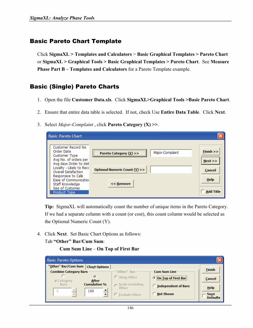
SigmaXL: Analyze Phase Tools
Basic Pareto Chart Template
Click SigmaXL > Templates and Calculators > Basic Graphical Templates > Pareto Chart
or SigmaXL > Graphical Tools > Basic Graphical Templates > Pareto Chart. See Measure
Phase Part B – Templates and Calculators for a Pareto Template example.
Basic (Single) Pareto Charts
1. Open the file Customer Data.xls. Click SigmaXL>Graphical Tools >Basic Pareto Chart.
2. Ensure that entire data table is selected. If not, check Use Entire Data Table. Click Next.
3. Select Major-Complaint , click Pareto Category (X) >>.
Tip: SigmaXL will automatically count the number of unique items in the Pareto Category.
If we had a separate column with a count (or cost), this count column would be selected as
the Optional Numeric Count (Y).
4. Click Next. Set Basic Chart Options as follows:
Tab “Other” Bar/Cum Sum:
Cum Sum Line – On Top of First Bar
146
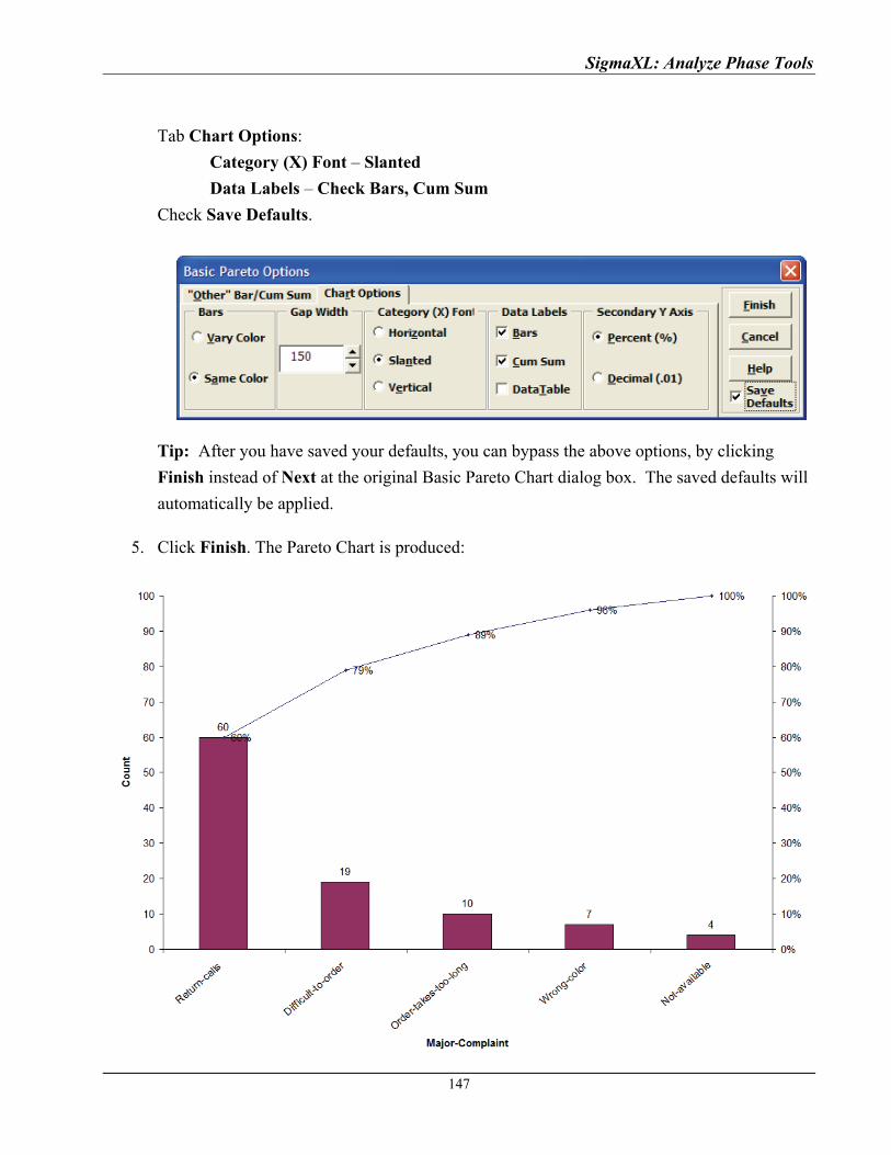
SigmaXL: Analyze Phase Tools
Tab Chart Options:
Category (X) Font – Slanted
Data Labels – Check Bars, Cum Sum
Check Save Defaults.
Tip: After you have saved your defaults, you can bypass the above options, by clicking
Finish instead of Next at the original Basic Pareto Chart dialog box. The saved defaults will
automatically be applied.
5. Click Finish. The Pareto Chart is produced:
147
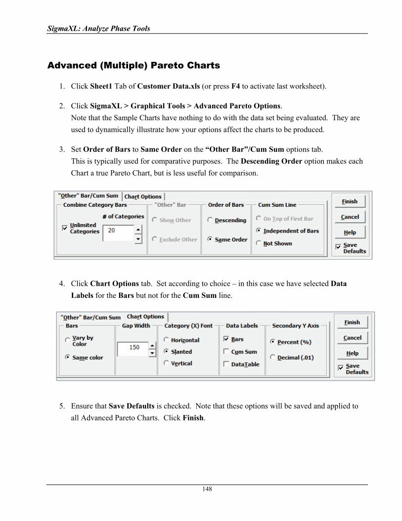
SigmaXL: Analyze Phase Tools
Advanced (Multiple) Pareto Charts
1. Click Sheet1 Tab of Customer Data.xls (or press F4 to activate last worksheet).
2. Click SigmaXL > Graphical Tools > Advanced Pareto Options.
Note that the Sample Charts have nothing to do with the data set being evaluated. They are
used to dynamically illustrate how your options affect the charts to be produced.
3. Set Order of Bars to Same Order on the “Other Bar”/Cum Sum options tab.
This is typically used for comparative purposes. The Descending Order option makes each
Chart a true Pareto Chart, but is less useful for comparison.
4. Click Chart Options tab. Set according to choice – in this case we have selected Data
Labels for the Bars but not for the Cum Sum line.
5. Ensure that Save Defaults is checked. Note that these options will be saved and applied to
all Advanced Pareto Charts. Click Finish.
148
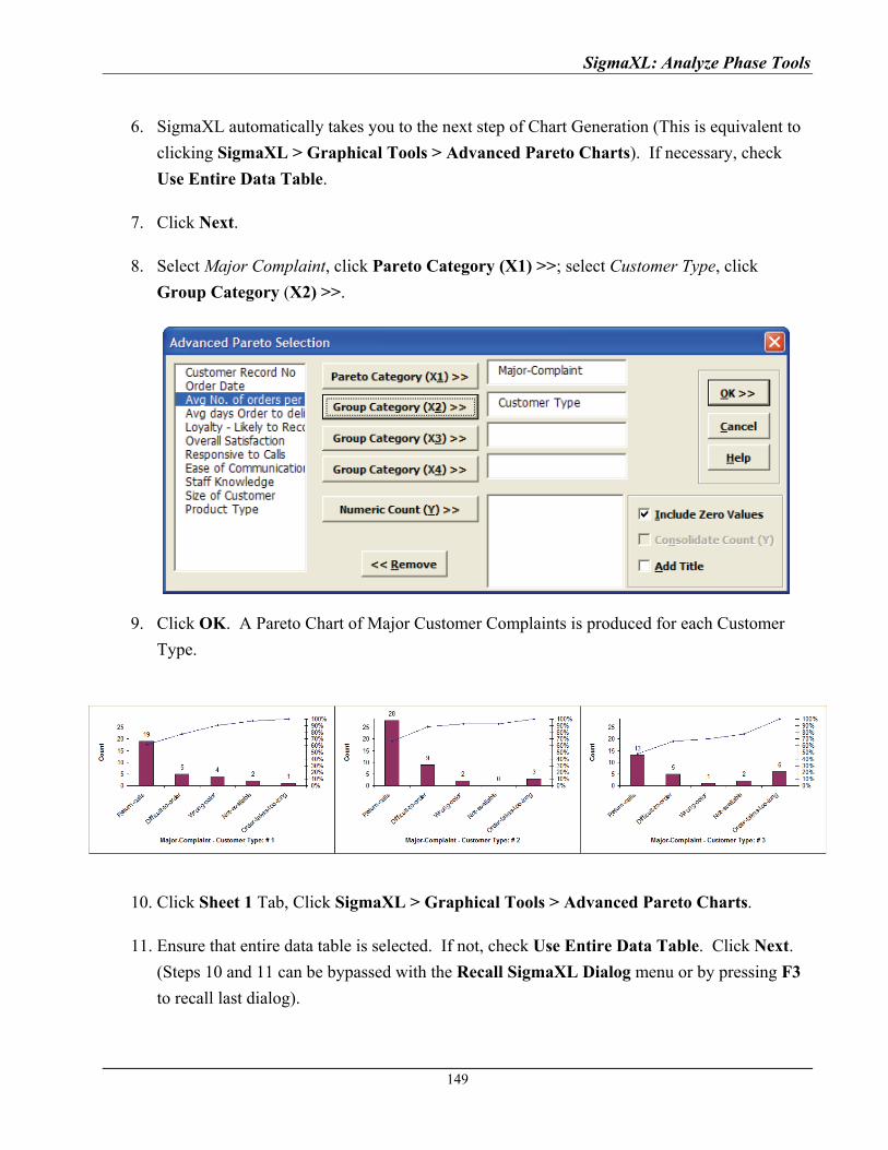
SigmaXL: Analyze Phase Tools
6. SigmaXL automatically takes you to the next step of Chart Generation (This is equivalent to
clicking SigmaXL > Graphical Tools > Advanced Pareto Charts). If necessary, check
Use Entire Data Table.
7. Click Next.
8. Select Major Complaint, click Pareto Category (X1) >>; select Customer Type, click
Group Category (X2) >>.
9. Click OK. A Pareto Chart of Major Customer Complaints is produced for each Customer
Type.
10. Click Sheet 1 Tab, Click SigmaXL > Graphical Tools > Advanced Pareto Charts.
11. Ensure that entire data table is selected. If not, check Use Entire Data Table. Click Next.
(Steps 10 and 11 can be bypassed with the Recall SigmaXL Dialog menu or by pressing F3
to recall last dialog).
149
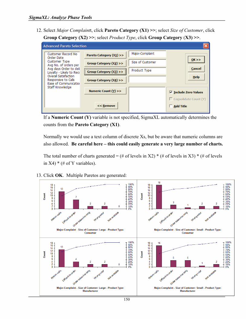
SigmaXL: Analyze Phase Tools
12. Select Major Complaintt, click Pareto Category (X1) >>; select Size of Customer, click
Group Category (X2) >>; select Product Type, click Group Category (X3) >>.
If a Numeric Count (Y) variable is not specified, SigmaXL automatically determines the
counts from the Pareto Category (X1).
Normally we would use a text column of discrete Xs, but be aware that numeric columns are
also allowed. Be careful here – this could easily generate a very large number of charts.
The total number of charts generated = (# of levels in X2) * (# of levels in X3) * (# of levels
in X4) * (# of Y variables).
13. Click OK. Multiple Paretos are generated:
150

SigmaXL: Analyze Phase Tools
Part B - EZ-Pivot
One of the most powerful features in Excel is the Pivot table. SigmaXL’s EZ-Pivot tool simplifies
the creation of Pivot tables using the familiar X and Y dialog box found in the previous Pareto tools.
Example of Three X’s, No Response Y’s
1. Open Customer Data.xls, click Sheet 1 (or press F4 to activate last worksheet). Select
SigmaXL > Graphical Tools > EZ-Pivot/Pivot Charts.
2. Ensure that entire data table is selected. If not, check Use Entire Data Table. Click Next.
3. Select Major Complaint, click Count Category (X1) >>. Note that if Y is not specified, the
Pivot Table Data is based on a count of X1, hence the name Count Category.
4. Select Customer Type, click Group Category (X2) >>; select Size of Customer, click Group
Category (X3) >> as shown.
5. Click OK. Resulting Pivot Table of Major Complaint by Customer Type is shown:
151
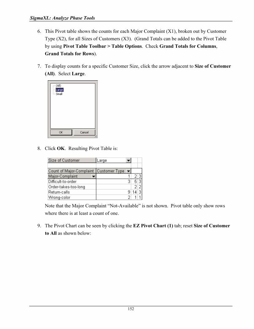
SigmaXL: Analyze Phase Tools
6. This Pivot table shows the counts for each Major Complaint (X1), broken out by Customer
Type (X2), for all Sizes of Customers (X3). (Grand Totals can be added to the Pivot Table
by using Pivot Table Toolbar > Table Options. Check Grand Totals for Columns,
Grand Totals for Rows).
7. To display counts for a specific Customer Size, click the arrow adjacent to Size of Customer
(All). Select Large.
8. Click OK. Resulting Pivot Table is:
Note that the Major Complaint “Not-Available” is not shown. Pivot table only show rows
where there is at least a count of one.
9. The Pivot Chart can be seen by clicking the EZ Pivot Chart (1) tab; reset Size of Customer
to All as shown below:
152
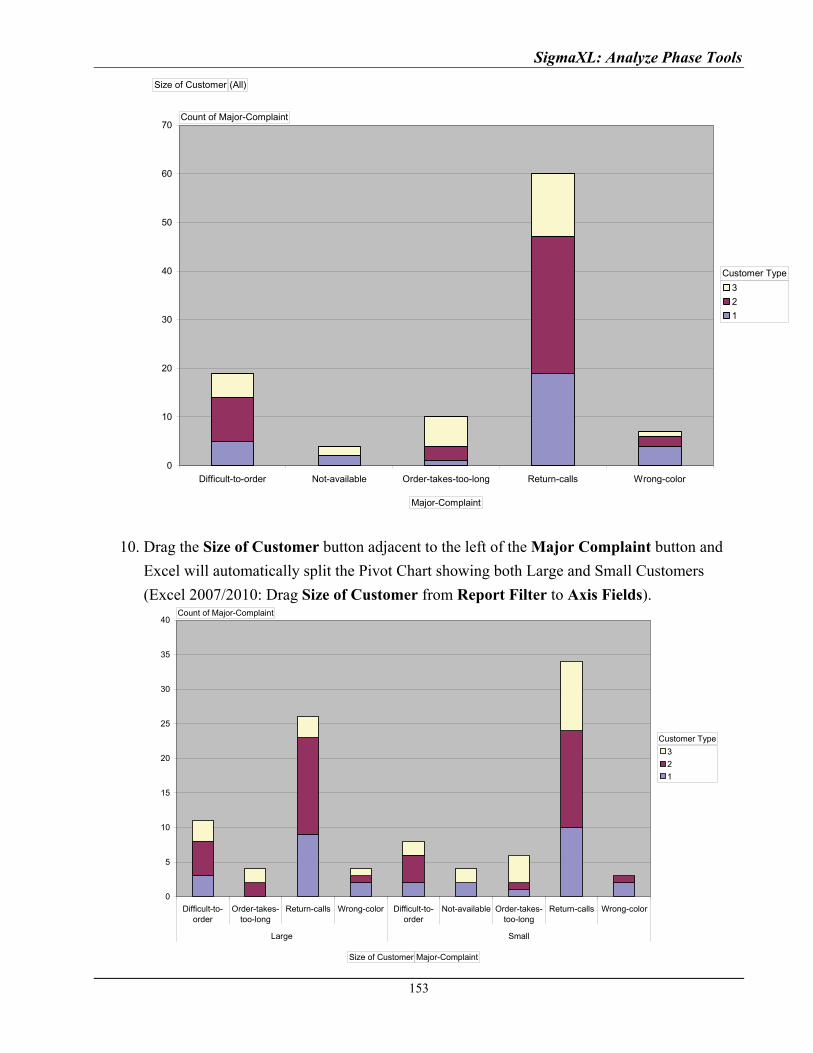
SigmaXL: Analyze Phase Tools
0
10
20
30
40
50
60
70
Difficult-to-order Not-available Order-takes-too-long Return-calls Wrong-color
3
2
1
Size of Customer (All)
Count of Major-Complaint
Major-Complaint
Customer Type
10. Drag the Size of Customer button adjacent to the left of the Major Complaint button and
Excel will automatically split the Pivot Chart showing both Large and Small Customers
(Excel 2007/2010: Drag Size of Customer from Report Filter to Axis Fields).
0
5
10
15
20
25
30
35
40
Difficult-to-order
Order-takes-too-long
Return-calls Wrong-color Difficult-to-order
Not-available Order-takes-too-long
Return-calls Wrong-color
Large Small
3
2
1
Count of Major-Complaint
Size of Customer Major-Complaint
Customer Type
153
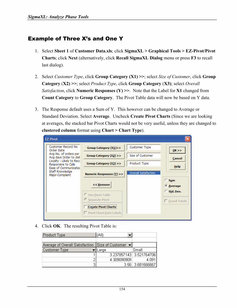
SigmaXL: Analyze Phase Tools
Example of Three X’s and One Y
1. Select Sheet 1 of Customer Data.xls; click SigmaXL > Graphical Tools > EZ-Pivot/Pivot
Charts; click Next (alternatively, click Recall SigmaXL Dialog menu or press F3 to recall
last dialog).
2. Select Customer Type, click Group Category (X1) >>; select Size of Customer, click Group
Category (X2) >>; select Product Type, click Group Category (X3); select Overall
Satisfaction, click Numeric Responses (Y) >>. Note that the Label for X1 changed from
Count Category to Group Category. The Pivot Table data will now be based on Y data.
3. The Response default uses a Sum of Y. This however can be changed to Average or
Standard Deviation. Select Average. Uncheck Create Pivot Charts (Since we are looking
at averages, the stacked bar Pivot Charts would not be very useful, unless they are changed to
clustered column format using Chart > Chart Type).
4. Click OK. The resulting Pivot Table is:
154

SigmaXL: Analyze Phase Tools
5. Note that the table now contains Averages of the Customer Satisfaction scores (Y). Again
Product Type (X3) can be varied to show Consumer, Manufacturer, or All. Double clicking
on Average of Overall Satisfaction allows you to switch to Standard Deviation (StdDev).
Example of 3 X’s and 3 Y’s
1. Click Recall SigmaXL Dialog menu or press F3 to recall last dialog.
2. Select Customer Type, click Group Category (X1) >>; select Size of Customer, click Group
Category (X2) >>; select Product Type, click Group Category (X3) >>. Select Avg Days
Order to Delivery, Loyalty – Likely to Respond, Overall Satisfaction, click Numeric
Responses (Y) >>. Select Average and One Pivot Table (default is separate Pivot Tables
for each Y). Uncheck Create Pivot Charts.
3. Click OK. Resulting Pivot Table:
Again, Product Type (X3) can be varied.
155
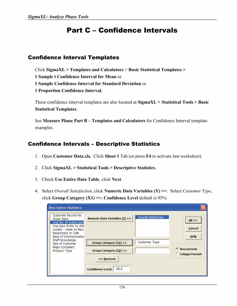
SigmaXL: Analyze Phase Tools
Part C – Confidence Intervals
Confidence Interval Templates
Click SigmaXL > Templates and Calculators > Basic Statistical Templates >
1 Sample t Confidence Interval for Mean or
1 Sample Confidence Interval for Standard Deviation or
1 Proportion Confidence Interval.
These confidence interval templates are also located at SigmaXL > Statistical Tools > Basic
Statistical Templates.
See Measure Phase Part B – Templates and Calculators for Confidence Interval template
examples.
Confidence Intervals – Descriptive Statistics
1. Open Customer Data.xls. Click Sheet 1 Tab (or press F4 to activate last worksheet).
2. Click SigmaXL > Statistical Tools > Descriptive Statistics.
3. Check Use Entire Data Table, click Next.
4. Select Overall Satisfaction, click Numeric Data Variables (Y) >>. Select Customer Type,
click Group Category (X1) >>; Confidence Level default is 95%:
156
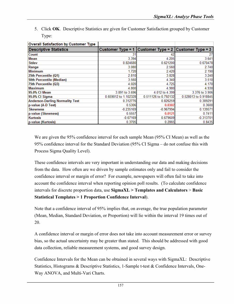
SigmaXL: Analyze Phase Tools
5. Click OK. Descriptive Statistics are given for Customer Satisfaction grouped by Customer
Type:
We are given the 95% confidence interval for each sample Mean (95% CI Mean) as well as the
95% confidence interval for the Standard Deviation (95% CI Sigma – do not confuse this with
Process Sigma Quality Level).
These confidence intervals are very important in understanding our data and making decisions
from the data. How often are we driven by sample estimates only and fail to consider the
confidence interval or margin of error? For example, newspapers will often fail to take into
account the confidence interval when reporting opinion poll results. (To calculate confidence
intervals for discrete proportion data, use SigmaXL > Templates and Calculators > Basic
Statistical Templates > 1 Proportion Confidence Interval).
Note that a confidence interval of 95% implies that, on average, the true population parameter
(Mean, Median, Standard Deviation, or Proportion) will lie within the interval 19 times out of
20.
A confidence interval or margin of error does not take into account measurement error or survey
bias, so the actual uncertainty may be greater than stated. This should be addressed with good
data collection, reliable measurement systems, and good survey design.
Confidence Intervals for the Mean can be obtained in several ways with SigmaXL: Descriptive
Statistics, Histograms & Descriptive Statistics, 1-Sample t-test & Confidence Intervals, One-
Way ANOVA, and Multi-Vari Charts.
157

SigmaXL: Analyze Phase Tools
To illustrate confidence intervals for the mean of Overall Satisfaction graphically, we have
generated a Multi-Vari Chart (with 95% CI Mean Options) using the Customer Data.xls data.
This chart type will be covered later (Part P).
The dots correspond to individual data points. The tick marks show the 95% upper confidence
limit, mean, and 95% lower confidence limit. Clearly we can see that Customer Type 2 has a
significantly higher level of mean satisfaction; the lower limit does not overlap with the upper
limit for Types 1 and 3. On the other hand, we see overlap of the CI’s when comparing types 1
and 3. Hypothesis testing will now be used to compare the mean satisfaction scores more
precisely and determine statistical significance for the results.
1
1.5
2
2.5
3
3.5
4
4.5
5
# 1 # 2 # 3
Customer Type
Ove
rall
Sat
isfa
ctio
n
(Mea
n O
pti
on
s)
158
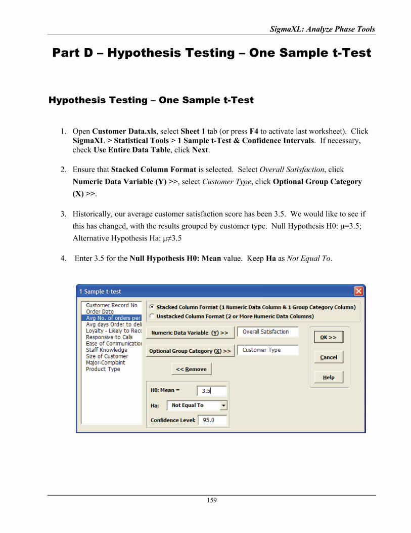
SigmaXL: Analyze Phase Tools
Part D – Hypothesis Testing – One Sample t-Test
Hypothesis Testing – One Sample t-Test
1. Open Customer Data.xls, select Sheet 1 tab (or press F4 to activate last worksheet). Click
SigmaXL > Statistical Tools > 1 Sample t-Test & Confidence Intervals. If necessary, check Use Entire Data Table, click Next.
2. Ensure that Stacked Column Format is selected. Select Overall Satisfaction, click
Numeric Data Variable (Y) >>, select Customer Type, click Optional Group Category
(X) >>.
3. Historically, our average customer satisfaction score has been 3.5. We would like to see if
this has changed, with the results grouped by customer type. Null Hypothesis H0: μ=3.5;
Alternative Hypothesis Ha: μ≠3.5
4. Enter 3.5 for the Null Hypothesis H0: Mean value. Keep Ha as Not Equal To.
159
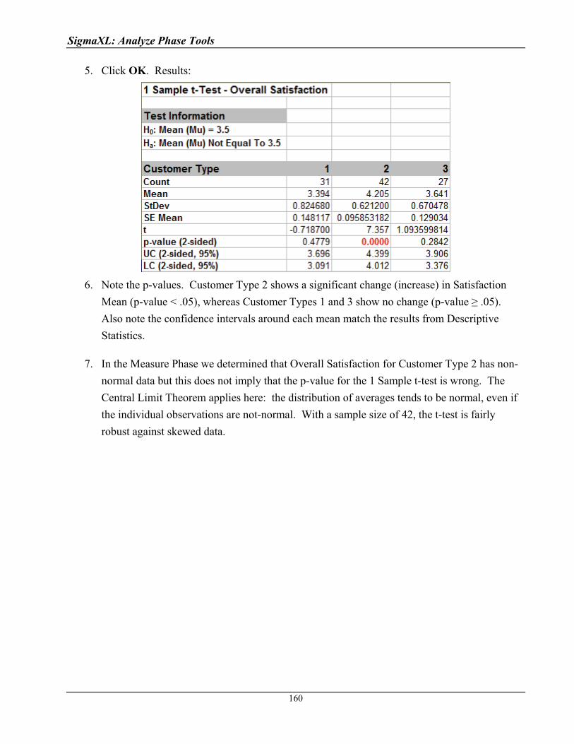
SigmaXL: Analyze Phase Tools
5. Click OK. Results:
6. Note the p-values. Customer Type 2 shows a significant change (increase) in Satisfaction
Mean (p-value < .05), whereas Customer Types 1 and 3 show no change (p-value ≥ .05).
Also note the confidence intervals around each mean match the results from Descriptive
Statistics.
7. In the Measure Phase we determined that Overall Satisfaction for Customer Type 2 has non-
normal data but this does not imply that the p-value for the 1 Sample t-test is wrong. The
Central Limit Theorem applies here: the distribution of averages tends to be normal, even if
the individual observations are not-normal. With a sample size of 42, the t-test is fairly
robust against skewed data.
160
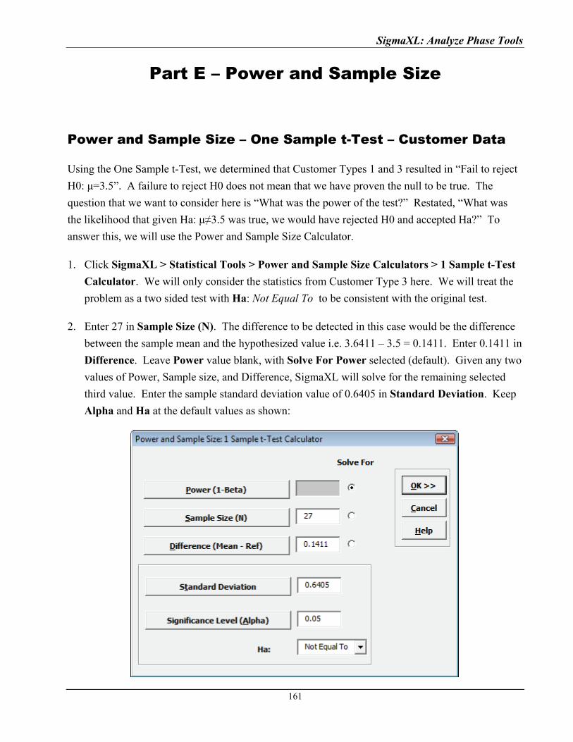
SigmaXL: Analyze Phase Tools
Part E – Power and Sample Size
Power and Sample Size – One Sample t-Test – Customer Data
Using the One Sample t-Test, we determined that Customer Types 1 and 3 resulted in “Fail to reject
H0: μ=3.5”. A failure to reject H0 does not mean that we have proven the null to be true. The
question that we want to consider here is “What was the power of the test?” Restated, “What was
the likelihood that given Ha: μ≠3.5 was true, we would have rejected H0 and accepted Ha?” To
answer this, we will use the Power and Sample Size Calculator.
1. Click SigmaXL > Statistical Tools > Power and Sample Size Calculators > 1 Sample t-Test
Calculator. We will only consider the statistics from Customer Type 3 here. We will treat the
problem as a two sided test with Ha: Not Equal To to be consistent with the original test.
2. Enter 27 in Sample Size (N). The difference to be detected in this case would be the difference
between the sample mean and the hypothesized value i.e. 3.6411 – 3.5 = 0.1411. Enter 0.1411 in
Difference. Leave Power value blank, with Solve For Power selected (default). Given any two
values of Power, Sample size, and Difference, SigmaXL will solve for the remaining selected
third value. Enter the sample standard deviation value of 0.6405 in Standard Deviation. Keep
Alpha and Ha at the default values as shown:
161
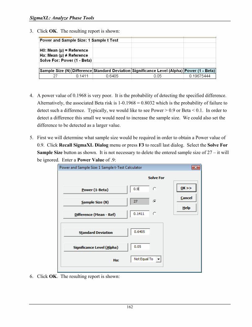
SigmaXL: Analyze Phase Tools
3. Click OK. The resulting report is shown:
4. A power value of 0.1968 is very poor. It is the probability of detecting the specified difference.
Alternatively, the associated Beta risk is 1-0.1968 = 0.8032 which is the probability of failure to
detect such a difference. Typically, we would like to see Power > 0.9 or Beta < 0.1. In order to
detect a difference this small we would need to increase the sample size. We could also set the
difference to be detected as a larger value.
5. First we will determine what sample size would be required in order to obtain a Power value of
0.9. Click Recall SigmaXL Dialog menu or press F3 to recall last dialog. Select the Solve For
Sample Size button as shown. It is not necessary to delete the entered sample size of 27 – it will
be ignored. Enter a Power Value of .9:
6. Click OK. The resulting report is shown:
162
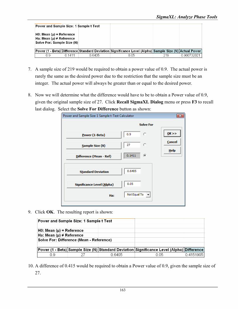
SigmaXL: Analyze Phase Tools
7. A sample size of 219 would be required to obtain a power value of 0.9. The actual power is
rarely the same as the desired power due to the restriction that the sample size must be an
integer. The actual power will always be greater than or equal to the desired power.
8. Now we will determine what the difference would have to be to obtain a Power value of 0.9,
given the original sample size of 27. Click Recall SigmaXL Dialog menu or press F3 to recall
last dialog. Select the Solve For Difference button as shown:
9. Click OK. The resulting report is shown:
10. A difference of 0.415 would be required to obtain a Power value of 0.9, given the sample size of
27.
163
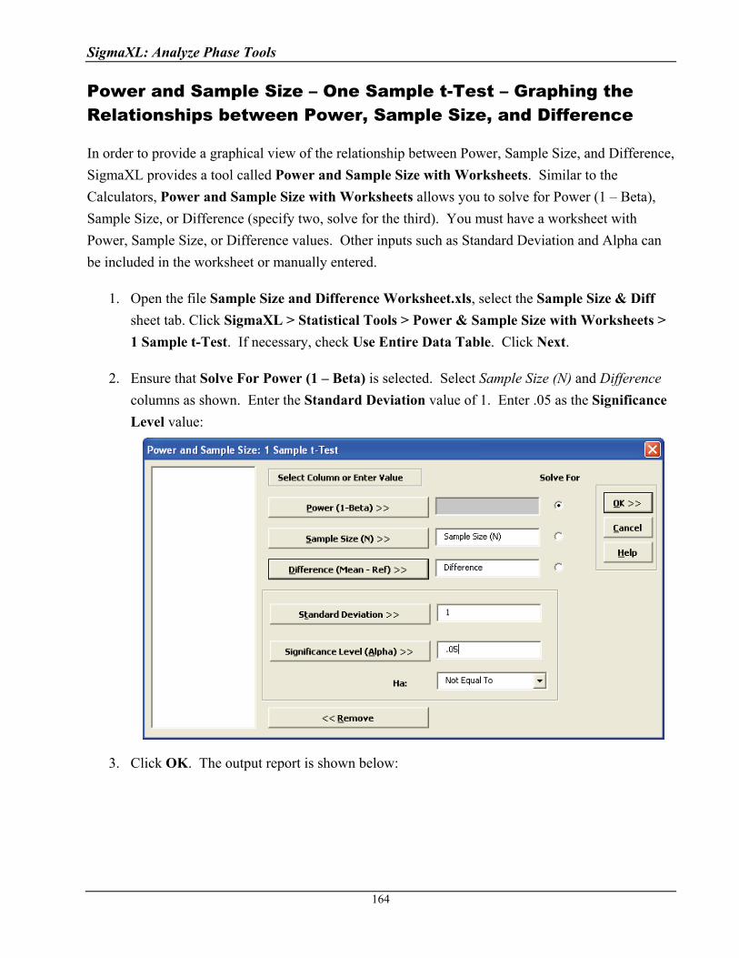
SigmaXL: Analyze Phase Tools
Power and Sample Size – One Sample t-Test – Graphing the Relationships between Power, Sample Size, and Difference
In order to provide a graphical view of the relationship between Power, Sample Size, and Difference,
SigmaXL provides a tool called Power and Sample Size with Worksheets. Similar to the
Calculators, Power and Sample Size with Worksheets allows you to solve for Power (1 – Beta),
Sample Size, or Difference (specify two, solve for the third). You must have a worksheet with
Power, Sample Size, or Difference values. Other inputs such as Standard Deviation and Alpha can
be included in the worksheet or manually entered.
1. Open the file Sample Size and Difference Worksheet.xls, select the Sample Size & Diff
sheet tab. Click SigmaXL > Statistical Tools > Power & Sample Size with Worksheets >
1 Sample t-Test. If necessary, check Use Entire Data Table. Click Next.
2. Ensure that Solve For Power (1 – Beta) is selected. Select Sample Size (N) and Difference
columns as shown. Enter the Standard Deviation value of 1. Enter .05 as the Significance
Level value:
3. Click OK. The output report is shown below:
164
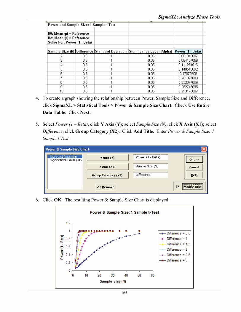
SigmaXL: Analyze Phase Tools
4. To create a graph showing the relationship between Power, Sample Size and Difference,
click SigmaXL > Statistical Tools > Power & Sample Size Chart. Check Use Entire
Data Table. Click Next.
5. Select Power (1 – Beta), click Y Axis (Y); select Sample Size (N), click X Axis (X1); select
Difference, click Group Category (X2). Click Add Title. Enter Power & Sample Size: 1
Sample t-Test:
6. Click OK. The resulting Power & Sample Size Chart is displayed:
165
SigmaXL: Analyze Phase Tools
166
Part F – One Sample Nonparametric Tests
Introduction to Nonparametric Tests
Nonparametric tests make fewer assumptions about the distribution of the data compared to
parametric tests like the t-Test. Nonparametric tests do not rely on the estimation of parameters such
as the mean or the standard deviation. They are sometimes called distribution-free tests.
Nonparametric tests use Medians and Ranks, thus they are robust to outliers in the data. If, however,
the data are normal and free of outliers, nonparametric tests are less powerful than normal based
tests to detect a real difference when one exists.
Nonparametric tests should be used when the data are non-normal, data cannot be readily
transformed to normality, and sample size is small (n < 30). If the sample sizes are large, the Central
Limit Theorem says that parametric tests are robust to non-normality.
One Sample Sign Test
The sign test is the simplest of the nonparametric tests, and is similar to testing if a two-sided coin is
fair. Count the number of positive values (larger than hypothesized median), the number of negative
values (smaller than the hypothesized median), and test whether there are significantly more
positives (or negatives) than expected. The One Sample Sign Test is a nonparametric equivalent to
the parametric One Sample t-Test.
Historically, our Median customer satisfaction score has been 3.5. We would like to see if this has
changed, with the results grouped by customer type (H0: Median=3.5, Ha: Median≠3.5, α = 0.05).
1. Open Customer Data.xls, select Sheet 1 tab. Click SigmaXL > Statistical Tools >
Nonparametric Tests>1 Sample Sign. If necessary, check Use Entire Data Table, click Next.
2. Ensure that Stacked Column Format is selected. Select Overall Satisfaction, click Numeric
Data Variable (Y) >>; select Customer Type, click Optional Group Category (X) >>.
3. Enter 3.5 for the Null Hypothesis H0: Median value. Set Ha as Not Equal To.

SigmaXL: Analyze Phase Tools
4. Click OK. Results:
5. Note the p-values. Customer Type 2 shows a significant change (increase) in Satisfaction
Median (p-value < .05), whereas Customer Types 1 and 3 show no change (p-value ≥ .05).
While the p-values are not the same as those given by the 1 sample t-Test, the conclusions do
match. we discussed that requires a nonparametric test.
One Sample Wilcoxon Signed Rank Test
The Wilcoxon Signed Rank test is a more powerful nonparametric test than the Sign Test, but it adds
an assumption that the distribution of values is symmetric around the median. An example of a
symmetric distribution is the uniform distribution. Symmetry can be observed with a histogram, or
by checking to see if the median and mean are approximately equal.
The One Sample Wilcoxon Test is a nonparametric equivalent to the parametric One Sample t-Test.
167
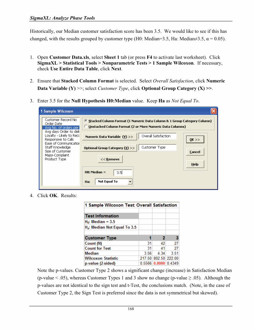
SigmaXL: Analyze Phase Tools
Historically, our Median customer satisfaction score has been 3.5. We would like to see if this has
changed, with the results grouped by customer type (H0: Median=3.5, Ha: Median≠3.5, α = 0.05).
1. Open Customer Data.xls, select Sheet 1 tab (or press F4 to activate last worksheet). Click
SigmaXL > Statistical Tools > Nonparametric Tests > 1 Sample Wilcoxon. If necessary, check Use Entire Data Table, click Next.
2. Ensure that Stacked Column Format is selected. Select Overall Satisfaction, click Numeric
Data Variable (Y) >>; select Customer Type, click Optional Group Category (X) >>.
3. Enter 3.5 for the Null Hypothesis H0:Median value. Keep Ha as Not Equal To.
4. Click OK. Results:
Note the p-values. Customer Type 2 shows a significant change (increase) in Satisfaction Median
(p-value < .05), whereas Customer Types 1 and 3 show no change (p-value ≥ .05). Although the
p-values are not identical to the sign test and t-Test, the conclusions match. (Note, in the case of
Customer Type 2, the Sign Test is preferred since the data is not symmetrical but skewed).
168
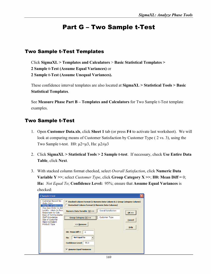
SigmaXL: Analyze Phase Tools
Part G – Two Sample t-Test
Two Sample t-Test Templates
Click SigmaXL > Templates and Calculators > Basic Statistical Templates >
2 Sample t-Test (Assume Equal Variances) or
2 Sample t-Test (Assume Unequal Variances).
These confidence interval templates are also located at SigmaXL > Statistical Tools > Basic
Statistical Templates.
See Measure Phase Part B – Templates and Calculators for Two Sample t-Test template
examples.
Two Sample t-Test
1. Open Customer Data.xls, click Sheet 1 tab (or press F4 to activate last worksheet). We will
look at comparing means of Customer Satisfaction by Customer Type ( 2 vs. 3), using the
Two Sample t-test. H0: μ2=μ3, Ha: μ2≠μ3
2. Click SigmaXL > Statistical Tools > 2 Sample t-test. If necessary, check Use Entire Data
Table, click Next.
3. With stacked column format checked, select Overall Satisfaction, click Numeric Data
Variable Y >>; select Customer Type, click Group Category X >>; H0: Mean Diff = 0;
Ha: Not Equal To; Confidence Level: 95%; ensure that Assume Equal Variances is
checked:
169
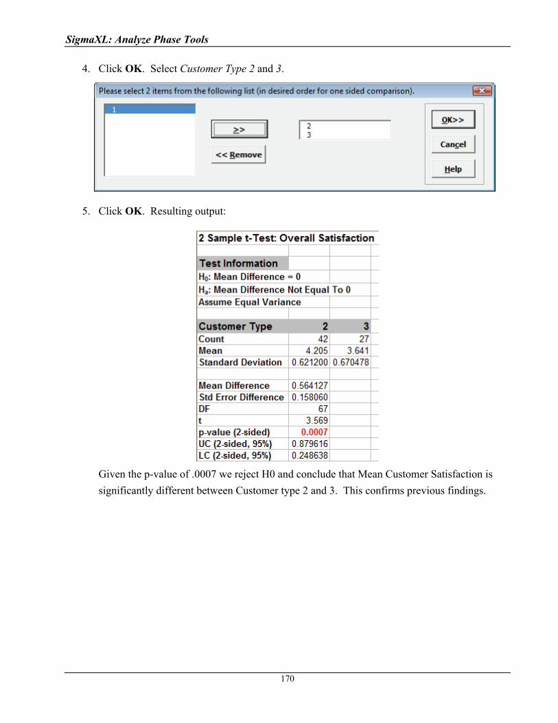
SigmaXL: Analyze Phase Tools
4. Click OK. Select Customer Type 2 and 3.
5. Click OK. Resulting output:
Given the p-value of .0007 we reject H0 and conclude that Mean Customer Satisfaction is
significantly different between Customer type 2 and 3. This confirms previous findings.
170
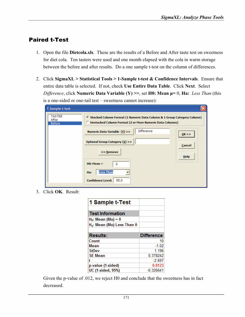
SigmaXL: Analyze Phase Tools
Paired t-Test
1. Open the file Dietcola.xls. These are the results of a Before and After taste test on sweetness
for diet cola. Ten tasters were used and one month elapsed with the cola in warm storage
between the before and after results. Do a one sample t-test on the column of differences.
2. Click SigmaXL > Statistical Tools > 1-Sample t-test & Confidence Intervals. Ensure that
entire data table is selected. If not, check Use Entire Data Table. Click Next. Select
Difference, click Numeric Data Variable (Y) >>, set H0: Mean μ= 0, Ha: Less Than (this
is a one-sided or one-tail test – sweetness cannot increase):
3. Click OK. Result:
Given the p-value of .012, we reject H0 and conclude that the sweetness has in fact
decreased.
171
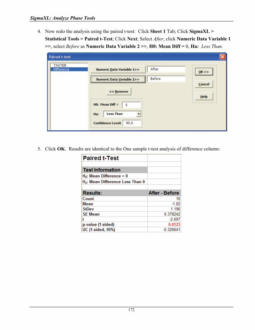
SigmaXL: Analyze Phase Tools
4. Now redo the analysis using the paired t-test: Click Sheet 1 Tab; Click SigmaXL >
Statistical Tools > Paired t-Test; Click Next; Select After, click Numeric Data Variable 1
>>, select Before as Numeric Data Variable 2 >>, H0: Mean Diff = 0, Ha: Less Than.
5. Click OK. Results are identical to the One sample t-test analysis of difference column:
172
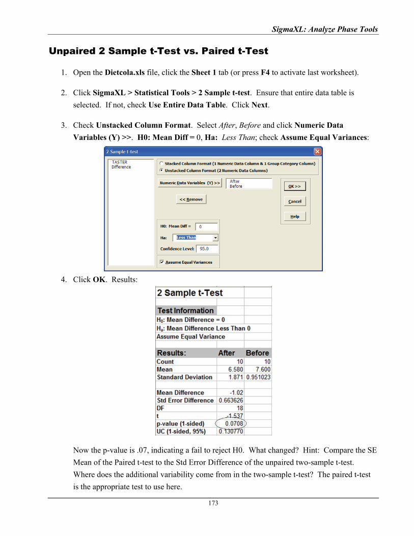
SigmaXL: Analyze Phase Tools
Unpaired 2 Sample t-Test vs. Paired t-Test
1. Open the Dietcola.xls file, click the Sheet 1 tab (or press F4 to activate last worksheet).
2. Click SigmaXL > Statistical Tools > 2 Sample t-test. Ensure that entire data table is
selected. If not, check Use Entire Data Table. Click Next.
3. Check Unstacked Column Format. Select After, Before and click Numeric Data
Variables (Y) >>. H0: Mean Diff = 0, Ha: Less Than; check Assume Equal Variances:
4. Click OK. Results:
Now the p-value is .07, indicating a fail to reject H0. What changed? Hint: Compare the SE
Mean of the Paired t-test to the Std Error Difference of the unpaired two-sample t-test.
Where does the additional variability come from in the two-sample t-test? The paired t-test
is the appropriate test to use here.
173

SigmaXL: Analyze Phase Tools
Power & Sample Size for 2 Sample T-Test
To determine Power & Sample Size for a 2 Sample t-Test, you can use the Power & Sample Size
Calculator or Power & Sample Size with Worksheet.
1. Click SigmaXL > Statistical Tools > Power & Sample Size Calculators > 2 Sample t-
Test Calculator.
2. Select Solve For Power (1 – Beta). Enter Sample Size and Difference as shown:
Note that we are calculating the power or likelihood of detection given that Mean1 – Mean2
= 1, with sample size for each group = 30, standard deviation = 1, significance level = .05,
and Ha: Not Equal To (two-sided test).
3. Click OK. The resulting report is displayed:
A power value of 0.97 is good, hence we have the basis for the “minimum sample size n=30”
rule of thumb used for continuous data.
174

SigmaXL: Analyze Phase Tools
175
4. To determine Power & Sample Size using a Worksheet, click SigmaXL > Statistical Tools
> Power & Sample Size with Worksheet > 2 Sample t-Test.
5. A graph showing the relationship between Power, Sample Size and Difference can then be
created using SigmaXL > Statistical Tools > Power & Sample Size Chart. See Part E for
an example using the 1 Sample t-Test.
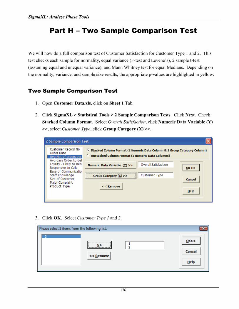
SigmaXL: Analyze Phase Tools
Part H – Two Sample Comparison Test
We will now do a full comparison test of Customer Satisfaction for Customer Type 1 and 2. This
test checks each sample for normality, equal variance (F-test and Levene’s), 2 sample t-test
(assuming equal and unequal variance), and Mann Whitney test for equal Medians. Depending on
the normality, variance, and sample size results, the appropriate p-values are highlighted in yellow.
Two Sample Comparison Test
1. Open Customer Data.xls, click on Sheet 1 Tab.
2. Click SigmaXL > Statistical Tools > 2 Sample Comparison Tests. Click Next. Check
Stacked Column Format. Select Overall Satisfaction, click Numeric Data Variable (Y)
>>, select Customer Type, click Group Category (X) >>.
3. Click OK. Select Customer Type 1 and 2.
176
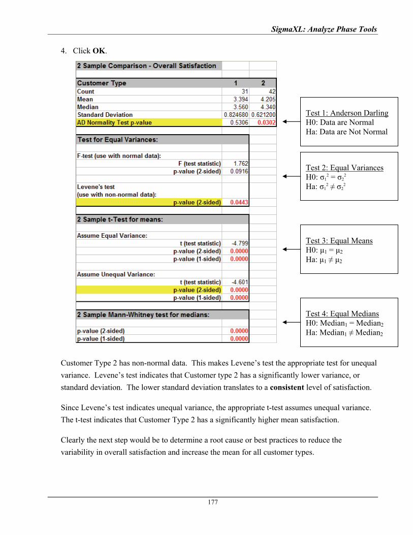
SigmaXL: Analyze Phase Tools
4. Click OK.
Test 1: Anderson Darling H0: Data are Normal Ha: Data are Not Normal
Test 2: Equal Variances H0: σ1
2 = σ22
Ha: σ12 ≠ σ2
2
Test 3: Equal Means H0: μ1 = μ2 Ha: μ1 ≠ μ2
Customer Type 2 has non-normal data. This makes Levene’s test the appropriate test for unequal
variance. Levene’s test indicates that Customer type 2 has a significantly lower variance, or
standard deviation. The lower standard deviation translates to a consistent level of satisfaction.
Test 4: Equal Medians H0: Median1 = Median2 Ha: Median1 ≠ Median2
Since Levene’s test indicates unequal variance, the appropriate t-test assumes unequal variance.
The t-test indicates that Customer Type 2 has a significantly higher mean satisfaction.
Clearly the next step would be to determine a root cause or best practices to reduce the
variability in overall satisfaction and increase the mean for all customer types.
177
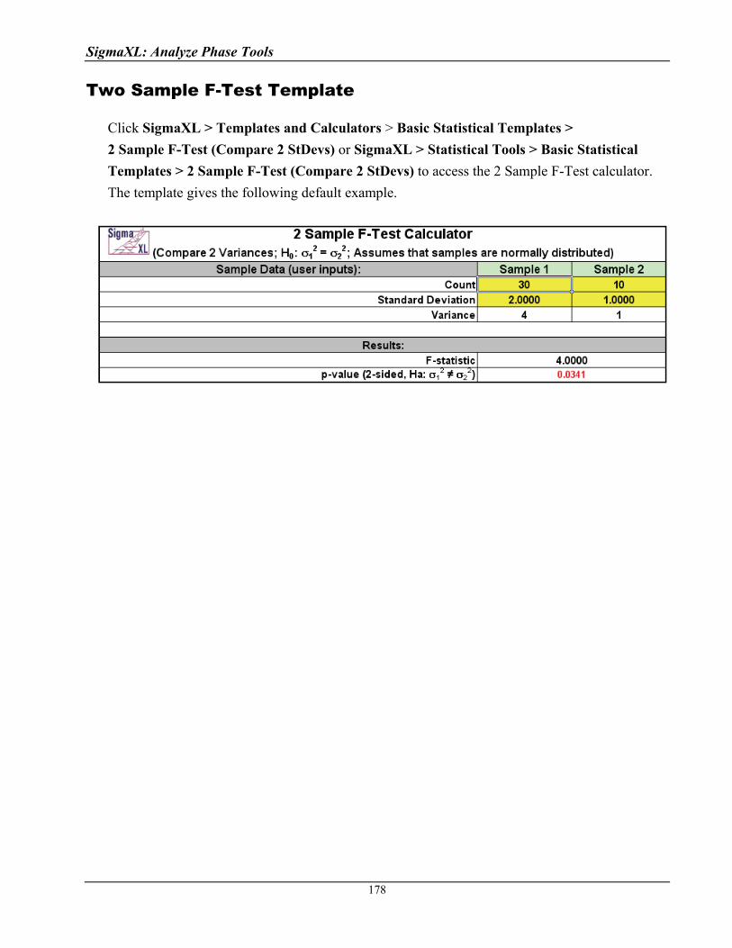
SigmaXL: Analyze Phase Tools
Two Sample F-Test Template
Click SigmaXL > Templates and Calculators > Basic Statistical Templates >
2 Sample F-Test (Compare 2 StDevs) or SigmaXL > Statistical Tools > Basic Statistical
Templates > 2 Sample F-Test (Compare 2 StDevs) to access the 2 Sample F-Test calculator.
The template gives the following default example.
178
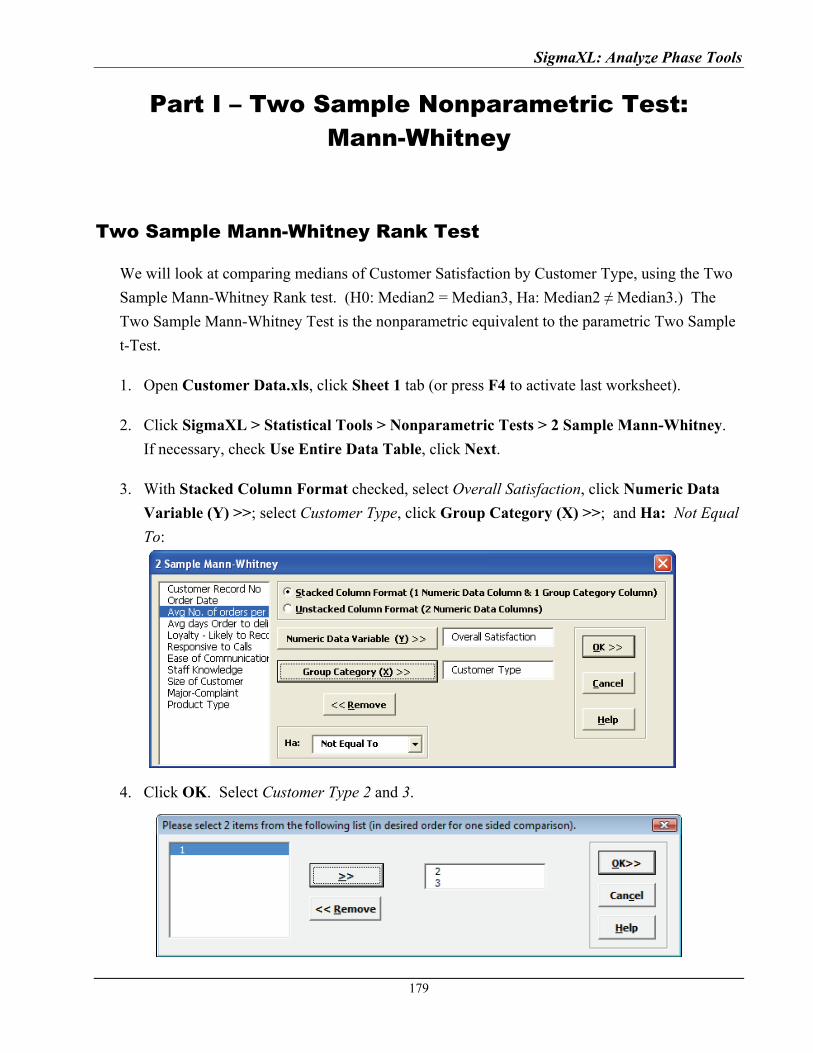
SigmaXL: Analyze Phase Tools
Part I – Two Sample Nonparametric Test: Mann-Whitney
Two Sample Mann-Whitney Rank Test
We will look at comparing medians of Customer Satisfaction by Customer Type, using the Two
Sample Mann-Whitney Rank test. (H0: Median2 = Median3, Ha: Median2 ≠ Median3.) The
Two Sample Mann-Whitney Test is the nonparametric equivalent to the parametric Two Sample
t-Test.
1. Open Customer Data.xls, click Sheet 1 tab (or press F4 to activate last worksheet).
2. Click SigmaXL > Statistical Tools > Nonparametric Tests > 2 Sample Mann-Whitney.
If necessary, check Use Entire Data Table, click Next.
3. With Stacked Column Format checked, select Overall Satisfaction, click Numeric Data
Variable (Y) >>; select Customer Type, click Group Category (X) >>; and Ha: Not Equal
To:
4. Click OK. Select Customer Type 2 and 3.
179
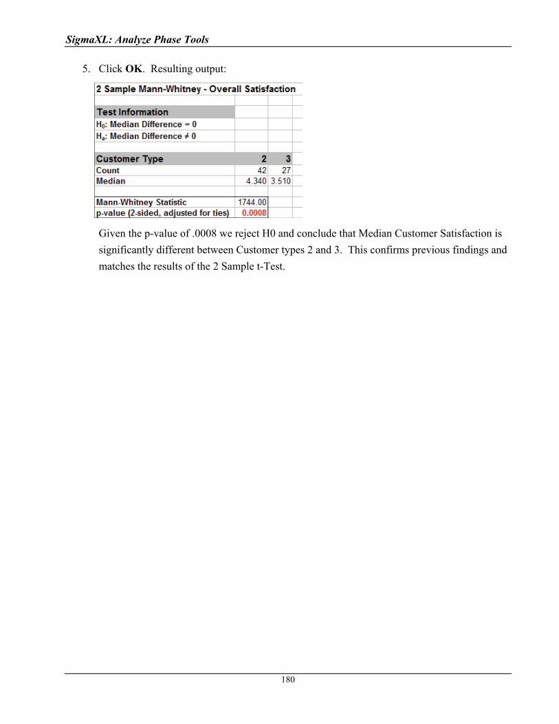
SigmaXL: Analyze Phase Tools
5. Click OK. Resulting output:
Given the p-value of .0008 we reject H0 and conclude that Median Customer Satisfaction is
significantly different between Customer types 2 and 3. This confirms previous findings and
matches the results of the 2 Sample t-Test.
180
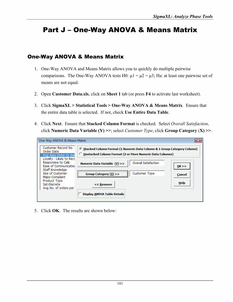
SigmaXL: Analyze Phase Tools
Part J – One-Way ANOVA & Means Matrix
One-Way ANOVA & Means Matrix
1. One-Way ANOVA and Means Matrix allows you to quickly do multiple pairwise
comparisons. The One-Way ANOVA tests H0: μ1 = μ2 = μ3; Ha: at least one pairwise set of
means are not equal.
2. Open Customer Data.xls, click on Sheet 1 tab (or press F4 to activate last worksheet).
3. Click SigmaXL > Statistical Tools > One-Way ANOVA & Means Matrix. Ensure that
the entire data table is selected. If not, check Use Entire Data Table.
4. Click Next. Ensure that Stacked Column Format is checked. Select Overall Satisfaction,
click Numeric Data Variable (Y) >>; select Customer Type, click Group Category (X) >>.
5. Click OK. The results are shown below:
181
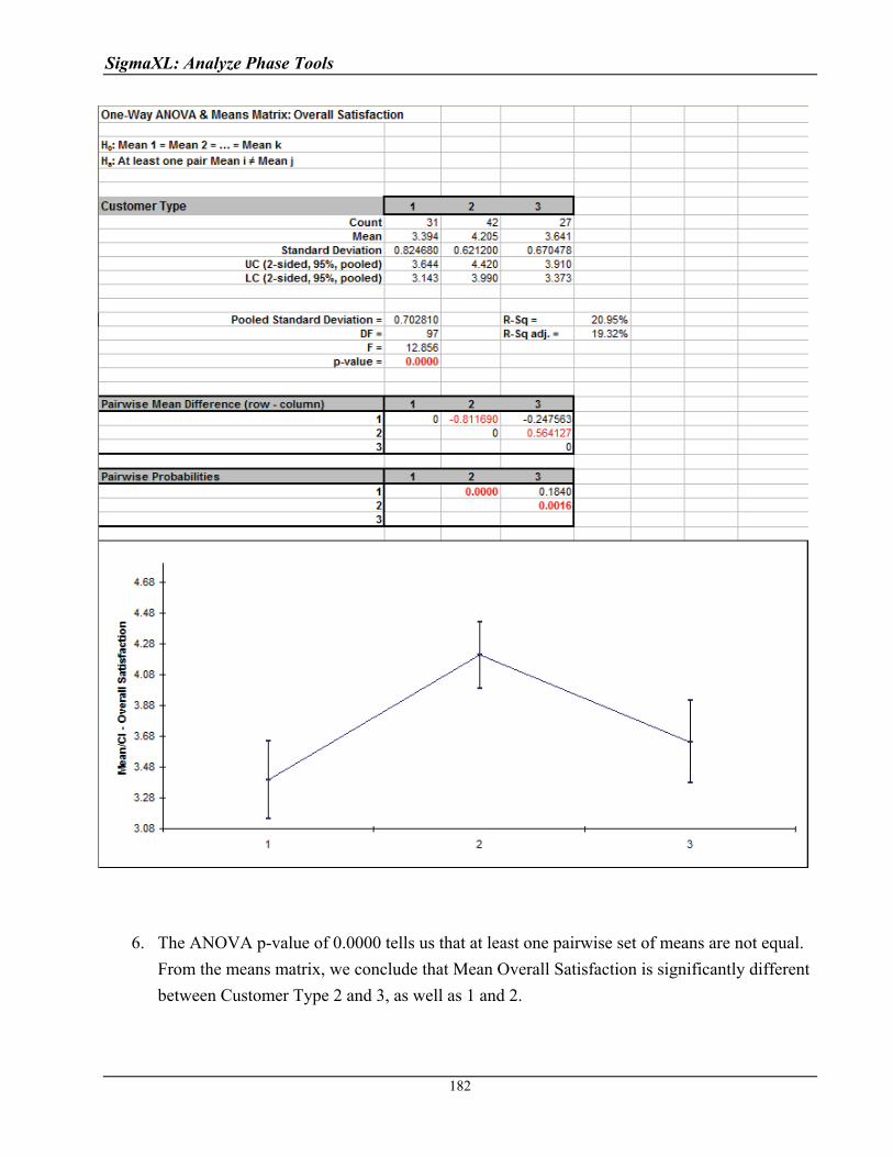
SigmaXL: Analyze Phase Tools
6. The ANOVA p-value of 0.0000 tells us that at least one pairwise set of means are not equal.
From the means matrix, we conclude that Mean Overall Satisfaction is significantly different
between Customer Type 2 and 3, as well as 1 and 2.
182

SigmaXL: Analyze Phase Tools
183
7. A graphical view of the Overall Satisfaction Mean and 95% Confidence Intervals are given
to complement the Means Matrix. The fact that the CI’s for Customer Type 2 do not overlap
those of Type 1 or 3, clearly shows that Customer Type 2 has a significantly higher mean
satisfaction score. The overlap of CI’s for Type 1 and 3 shows that the mean satisfaction
scores for 1 and 3 are not significantly different.
8. The R-Square (R-Sq) value of 20.95% indicates that Customer type “explains”
approximately 21% of the variation in Overall Satisfaction. We need to “drill down” to
understand the root causes and best practices associated with Customer Type 2.
9. Note that the p-value for 2-3 is slightly different than the previous two sample test result
because the variances from all 3 customer types are “pooled” here. This also results in
slightly different confidence intervals. One-Way ANOVA & Means Matrix assume equal
variance, but analysis above in Part H indicates that this assumption is not true, so this
analysis should be treated with caution. An alternative nonparametric test is the Kruskal-
Wallis test for Medians (SigmaXL > Statistical Tools > Nonparametric Tests > Kruskal-
Wallis Median Test) or Mood’s Median (SigmaXL > Statistical Tools > Nonparametric
Tests > Mood’s Median Test). These are discussed in Part M.
Note also that the means matrix p-values could easily trigger type I errors when the number
of X levels gets large. You should only consider the results of the Means Matrix if the
ANOVA p-value is < .05.

SigmaXL: Analyze Phase Tools
Power & Sample Size for One-Way ANOVA
To determine Power & Sample Size for a One-Way ANOVA, you can use the Power & Sample
Size Calculator or Power & Sample Size with Worksheet.
1. Click SigmaXL > Statistical Tools > Power & Sample Size Calculators > One-Way
ANOVA Calculator.
2. Select Solve For Power (1 – Beta). Enter Sample Size and Maximum Difference as
shown:
Note that we are calculating the power or likelihood of detection given that the maximum
difference between group means = 1, with sample size for each group = 30, 3 groups,
standard deviation = 1, significance level = .05, and Ha: Not Equal To (two sided test).
3. Click OK. The resulting report is displayed:
184
SigmaXL: Analyze Phase Tools
185
A power value of 0.94 is acceptable. Note that this value is less than the power value of 0.97
obtained with the two-sample t-Test.
4. Press F3 or click Recall SigmaXL Dialog to recall last dialog. Change the number of
groups to 4. Note that the power value is 0.907. If the number of groups (levels) increases,
you will have to increase the sample size in order to maintain statistical power.
5. To determine Power & Sample Size using a Worksheet, click SigmaXL > Statistical Tools
> Power & Sample Size with Worksheet > One-Way ANOVA.
6. A graph showing the relationship between Power, Sample Size and Maximum Difference can
then be created using SigmaXL > Statistical Tools > Power & Sample Size Chart. See
Part E for an example using the 1 Sample t-Test.
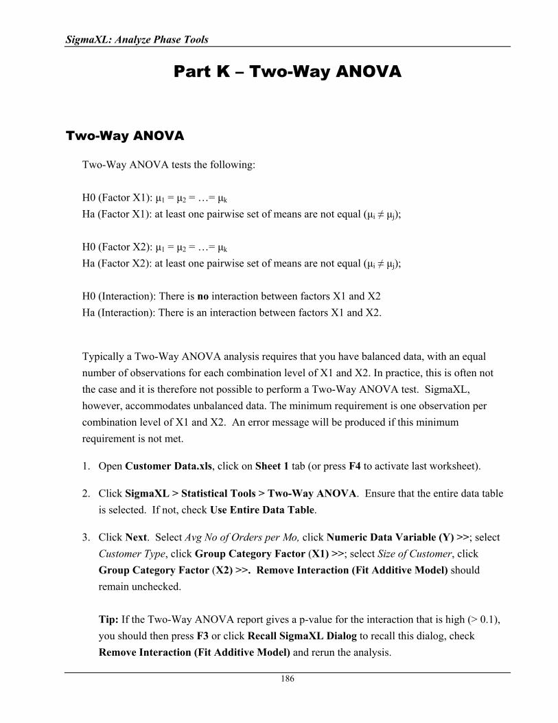
SigmaXL: Analyze Phase Tools
186
Part K – Two-Way ANOVA
Two-Way ANOVA
Two-Way ANOVA tests the following:
H0 (Factor X1): μ1 = μ2 = …= μk
Ha (Factor X1): at least one pairwise set of means are not equal (μi ≠ μj);
H0 (Factor X2): μ1 = μ2 = …= μk
Ha (Factor X2): at least one pairwise set of means are not equal (μi ≠ μj);
H0 (Interaction): There is no interaction between factors X1 and X2
Ha (Interaction): There is an interaction between factors X1 and X2.
Typically a Two-Way ANOVA analysis requires that you have balanced data, with an equal
number of observations for each combination level of X1 and X2. In practice, this is often not
the case and it is therefore not possible to perform a Two-Way ANOVA test. SigmaXL,
however, accommodates unbalanced data. The minimum requirement is one observation per
combination level of X1 and X2. An error message will be produced if this minimum
requirement is not met.
1. Open Customer Data.xls, click on Sheet 1 tab (or press F4 to activate last worksheet).
2. Click SigmaXL > Statistical Tools > Two-Way ANOVA. Ensure that the entire data table
is selected. If not, check Use Entire Data Table.
3. Click Next. Select Avg No of Orders per Mo, click Numeric Data Variable (Y) >>; select
Customer Type, click Group Category Factor (X1) >>; select Size of Customer, click
Group Category Factor (X2) >>. Remove Interaction (Fit Additive Model) should
remain unchecked.
Tip: If the Two-Way ANOVA report gives a p-value for the interaction that is high (> 0.1),
you should then press F3 or click Recall SigmaXL Dialog to recall this dialog, check
Remove Interaction (Fit Additive Model) and rerun the analysis.
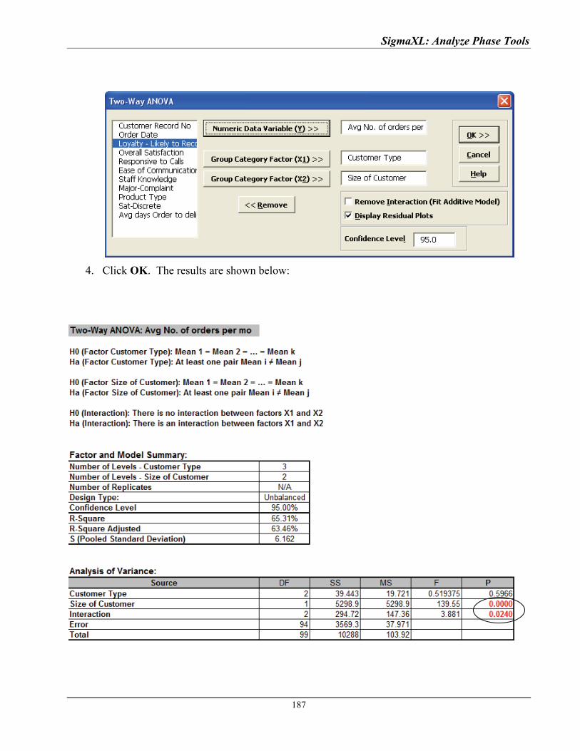
SigmaXL: Analyze Phase Tools
4. Click OK. The results are shown below:
187
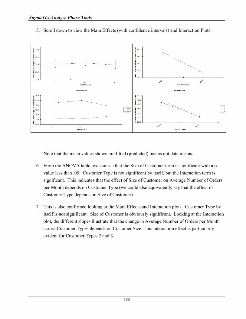
SigmaXL: Analyze Phase Tools
5. Scroll down to view the Main Effects (with confidence intervals) and Interaction Plots:
Note that the mean values shown are fitted (predicted) means not data means.
6. From the ANOVA table, we can see that the Size of Customer term is significant with a p-
value less than .05. Customer Type is not significant by itself, but the Interaction term is
significant. This indicates that the effect of Size of Customer on Average Number of Orders
per Month depends on Customer Type (we could also equivalently say that the effect of
Customer Type depends on Size of Customer).
7. This is also confirmed looking at the Main Effects and Interaction plots. Customer Type by
itself is not significant. Size of Customer is obviously significant. Looking at the Interaction
plot, the different slopes illustrate that the change in Average Number of Orders per Month
across Customer Types depends on Customer Size. This interaction effect is particularly
evident for Customer Types 2 and 3.
188
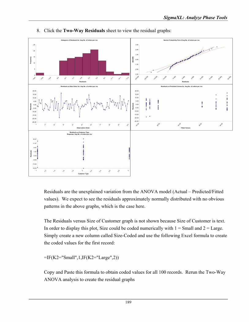
SigmaXL: Analyze Phase Tools
8. Click the Two-Way Residuals sheet to view the residual graphs:
Residuals are the unexplained variation from the ANOVA model (Actual – Predicted/Fitted
values). We expect to see the residuals approximately normally distributed with no obvious
patterns in the above graphs, which is the case here.
The Residuals versus Size of Customer graph is not shown because Size of Customer is text.
In order to display this plot, Size could be coded numerically with 1 = Small and 2 = Large.
Simply create a new column called Size-Coded and use the following Excel formula to create
the coded values for the first record:
=IF(K2="Small",1,IF(K2="Large",2))
Copy and Paste this formula to obtain coded values for all 100 records. Rerun the Two-Way
ANOVA analysis to create the residual graphs
189
Histogram of Residuals for: Avg No. of orders per mo
.6-1
2.6 -9.6
-6.7
-3.7
-0.8 2.
25.
28.
111
.114
.117
.0
Residuals
0
5
10
15
20
25
-18.5
-15
Fre
qu
ency
Normal Probability Plot of Avg No. of orders per mo
-3.00
-2.00
-1.00
0.00
1.00
2.00
3.00
-25.0
00
-20.0
00
-15.0
00
-10.0
00
-5.00
0
0.00
05.
000
10.00
0
15.00
0
20.00
0
25.00
0
Residuals
NS
CO
RE
Residuals vs Predicted Values for: Avg No. of orders per mo
-25.00
-20.00
-15.00
-10.00
-5.00
0.00
5.00
10.00
15.00
20.00
24.00
29.00
34.00
39.00
44.00
Fitted Values
Res
idu
als
Residuals vs Data Order for: Avg No. of orders per mo
11 21 31 41 51 61 71 81 91 101
Observation Order
-25.00
-20.00
-15.00
-10.00
-5.00
0.00
5.00
10.00
15.00
20.00
1
Res
idu
als
Residuals vs Customer TypeResponse: Avg No. of orders per mo
1.2
1.4
1.6
1.8 2
2.2
2.4
2.6
2.8 3
Customer Type
-18.54
-13.54
-8.54
-3.54
1.47
6.47
11.47
16.47
1
Res
idu
als

SigmaXL: Analyze Phase Tools
Part L – Tests for Equal Variance & Welch’s ANOVA
Bartlett’s Test
Bartlett’s Test is similar to the 2 sample F-Test (SigmaXL > Statistical Tools > 2 Sample
Comparison Test) but allows for multiple group comparison of variances (or standard deviations).
Like the F-Test, Bartlett’s requires that the data from each group be normally distributed but is more
powerful than Levene’s Test.
1. Open Delivery Times.xls, click on Sheet 1 tab.
2. Click SigmaXL > Statistical Tools > Equal Variance Tests > Bartlett. Ensure that the
entire data table is selected. If not, check Use Entire Data Table.
3. Click Next. Ensure that Stacked Column Format is checked. Select Delivery Time
Deviation, click Numeric Data Variable (Y) >>; select Floor, click Group Category (X)
>>.
4. Click OK. The results are shown below:
190

SigmaXL: Analyze Phase Tools
5. With the p-value = 0.63 we fail to reject H0; we do not have evidence to show that the group
variances are unequal (practically speaking we will assume that the variances are equal).
6. All 10 Anderson-Darling Test P-values are > .05 indicating that all group data are normal.
Since the assumption of normality is met, Bartlett’s is the appropriate test to use. If any one
of the groups have a low p-value for the Normality test, then Levene’s test should be used.
Levene’s Test
Levene’s Test for multiple group comparison of variances is less powerful that Bartlett’s Test, but is
robust to the assumption of normality. (This is a modification of the original Levene’s Test,
sometimes referred to as the Browne-Forsythe Test).
1. Open Customer Data.xls, click on Sheet 1 tab.
2. Click SigmaXL > Statistical Tools > Equal Variance Tests > Levene. Ensure that the
entire data table is selected. If not, check Use Entire Data Table.
3. Click Next. Ensure that Stacked Column Format is checked. Select Responsive to Calls,
click Numeric Data Variable (Y) >>; select Customer Type, click Group Category (X) >>.
4. Click OK. The results are shown below:
191
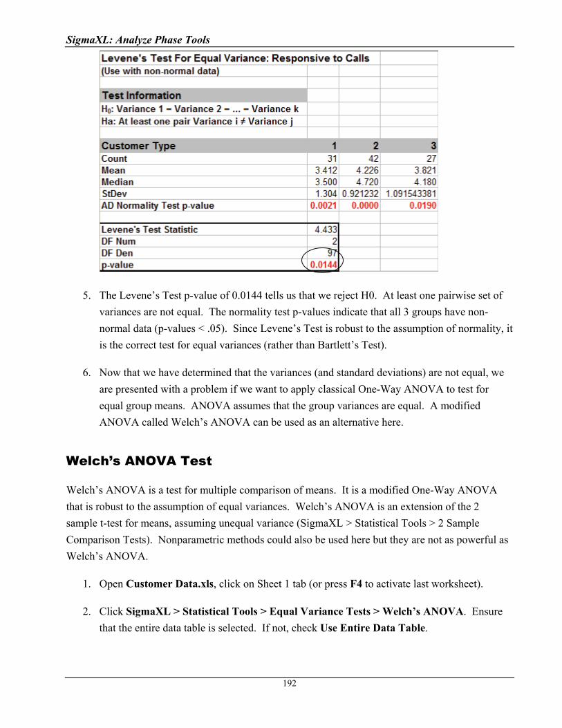
SigmaXL: Analyze Phase Tools
5. The Levene’s Test p-value of 0.0144 tells us that we reject H0. At least one pairwise set of
variances are not equal. The normality test p-values indicate that all 3 groups have non-
normal data (p-values < .05). Since Levene’s Test is robust to the assumption of normality, it
is the correct test for equal variances (rather than Bartlett’s Test).
6. Now that we have determined that the variances (and standard deviations) are not equal, we
are presented with a problem if we want to apply classical One-Way ANOVA to test for
equal group means. ANOVA assumes that the group variances are equal. A modified
ANOVA called Welch’s ANOVA can be used as an alternative here.
Welch’s ANOVA Test
Welch’s ANOVA is a test for multiple comparison of means. It is a modified One-Way ANOVA
that is robust to the assumption of equal variances. Welch’s ANOVA is an extension of the 2
sample t-test for means, assuming unequal variance (SigmaXL > Statistical Tools > 2 Sample
Comparison Tests). Nonparametric methods could also be used here but they are not as powerful as
Welch’s ANOVA.
1. Open Customer Data.xls, click on Sheet 1 tab (or press F4 to activate last worksheet).
2. Click SigmaXL > Statistical Tools > Equal Variance Tests > Welch’s ANOVA. Ensure
that the entire data table is selected. If not, check Use Entire Data Table.
192

SigmaXL: Analyze Phase Tools
3. Click Next. Ensure that Stacked Column Format is checked. Select Responsive to Calls,
click Numeric Data Variable (Y) >>; select Customer Type, click Group Category (X) >>.
4. Click OK. The results are shown below:
5. The p-value for Welch’s ANOVA is 0.0135, therefore we reject H0 and conclude that the
group means for Responsive to Calls are not equal. We will explore the relationship between
Overall Satisfaction and Responsive to Calls later.
193
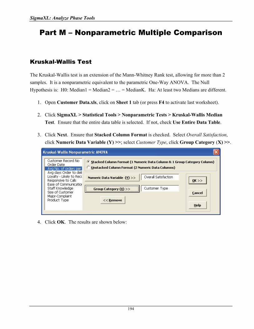
SigmaXL: Analyze Phase Tools
Part M – Nonparametric Multiple Comparison
Kruskal-Wallis Test
The Kruskal-Wallis test is an extension of the Mann-Whitney Rank test, allowing for more than 2
samples. It is a nonparametric equivalent to the parametric One-Way ANOVA. The Null
Hypothesis is: H0: Median1 = Median2 = … = MedianK. Ha: At least two Medians are different.
1. Open Customer Data.xls, click on Sheet 1 tab (or press F4 to activate last worksheet).
2. Click SigmaXL > Statistical Tools > Nonparametric Tests > Kruskal-Wallis Median
Test. Ensure that the entire data table is selected. If not, check Use Entire Data Table.
3. Click Next. Ensure that Stacked Column Format is checked. Select Overall Satisfaction,
click Numeric Data Variable (Y) >>; select Customer Type, click Group Category (X) >>.
4. Click OK. The results are shown below:
194

SigmaXL: Analyze Phase Tools
The p-value of 0.0000 tells us that we reject H0. At least one pairwise set of medians are not
equal.
5. The Kruskal-Wallis Statistic is based on comparing mean ranks for each group versus the
mean rank for all observations. The Z value for Customer Type 3 is , the smallest
absolute Z-value. This size indicates that the mean rank for Type 3 differed least from the
mean rank for all observations. The Z value for Customer Type 2 is 4.53, the largest absolute
Z-value. This size indicates that the mean rank differed most from the mean rank for all
observations.
195

SigmaXL: Analyze Phase Tools
6. A graphical view of the Overall Satisfaction Median and 95% Confidence Intervals are given
to complement the Z scores. The fact that the CI’s for Customer Type 2 do not overlap those
of Type 1 or 3, clearly shows that Customer Type 2 has a significantly higher median
satisfaction score. The overlap of CI’s for Type 1 and 3 shows that the median satisfaction
scores for 1 and 3 are not significantly different.
Mood’s Median Test
Mood’s Median Test is an extension of the One Sample Sign Test, using Chi-Square as the test
statistic. Like the Kruskal-Wallis test, Mood's median test can be used to test the equality of
medians from multiple samples. It provides a nonparametric alternative to the one-way analysis of
variance. The Null Hypothesis is: H0: Median1 = Median2 = … = MedianK. Ha: At least two
Medians are different.
Mood's median test is more robust to outliers than the Kruskal-Wallis test, but is less powerful in the
absence of outliers. You should first look at your data with Boxplots. If there are extreme outliers,
then Mood’s Median should be used rather than Kruskal-Wallis.
1. Open Customer Data.xls, click on Sheet 1 tab (or press F4 to activate last worksheet).
2. Click SigmaXL > Statistical Tools > Nonparametric Tests > Mood’s Median Test.
Ensure that the entire data table is selected. If not, check Use Entire Data Table.
3. Click Next. Ensure that Stacked Column Format is checked. Select Overall Satisfaction,
click Numeric Data Variable (Y) >>; select Customer Type, click Group Category (X) >>.
4. Click OK. The results are shown below:
196
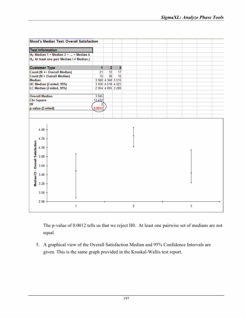
SigmaXL: Analyze Phase Tools
197
The p-value of 0.0012 tells us that we reject H0. At least one pairwise set of medians are not
equal.
5. A graphical view of the Overall Satisfaction Median and 95% Confidence Intervals are
given. This is the same graph provided in the Kruskal-Wallis test report.
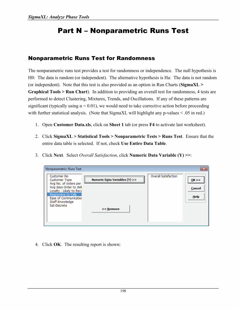
SigmaXL: Analyze Phase Tools
Part N – Nonparametric Runs Test
Nonparametric Runs Test for Randomness
The nonparametric runs test provides a test for randomness or independence. The null hypothesis is
H0: The data is random (or independent). The alternative hypothesis is Ha: The data is not random
(or independent). Note that this test is also provided as an option in Run Charts (SigmaXL >
Graphical Tools > Run Chart). In addition to providing an overall test for randomness, 4 tests are
performed to detect Clustering, Mixtures, Trends, and Oscillations. If any of these patterns are
significant (typically using α = 0.01), we would need to take corrective action before proceeding
with further statistical analysis. (Note that SigmaXL will highlight any p-values < .05 in red.)
1. Open Customer Data.xls, click on Sheet 1 tab (or press F4 to activate last worksheet).
2. Click SigmaXL > Statistical Tools > Nonparametric Tests > Runs Test. Ensure that the
entire data table is selected. If not, check Use Entire Data Table.
3. Click Next. Select Overall Satisfaction, click Numeric Data Variable (Y) >>:
4. Click OK. The resulting report is shown:
198

SigmaXL: Analyze Phase Tools
5. With all of the p-values being greater than 0.01, we fail to reject H0, and conclude that the
data is random (or statistically independent). Recall from the run chart of this data that there
were no obvious trends or patterns.
6. Examples of Clustering, Mixtures, Trends, and Oscillations are given below using the Run
Chart to illustrate. The data for these examples are given in the file Runs Test Example
Data.xls. (Use SigmaXL > Graphical Tools > Run Charts to create the run charts).
a. Clustering appears as a group of points in one area of the chart. It may indicate
special cause variation such as sampling or measurement problems.
199
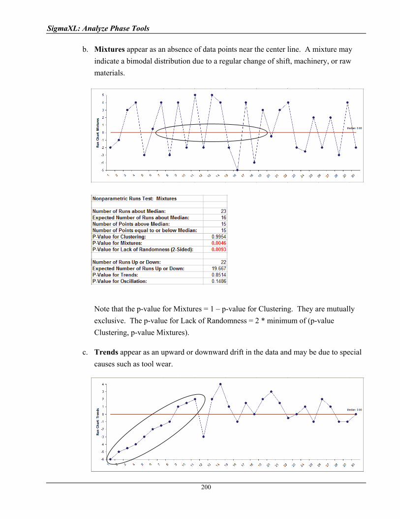
SigmaXL: Analyze Phase Tools
b. Mixtures appear as an absence of data points near the center line. A mixture may
indicate a bimodal distribution due to a regular change of shift, machinery, or raw
materials.
Note that the p-value for Mixtures = 1 – p-value for Clustering. They are mutually
exclusive. The p-value for Lack of Randomness = 2 * minimum of (p-value
Clustering, p-value Mixtures).
c. Trends appear as an upward or downward drift in the data and may be due to special
causes such as tool wear.
200
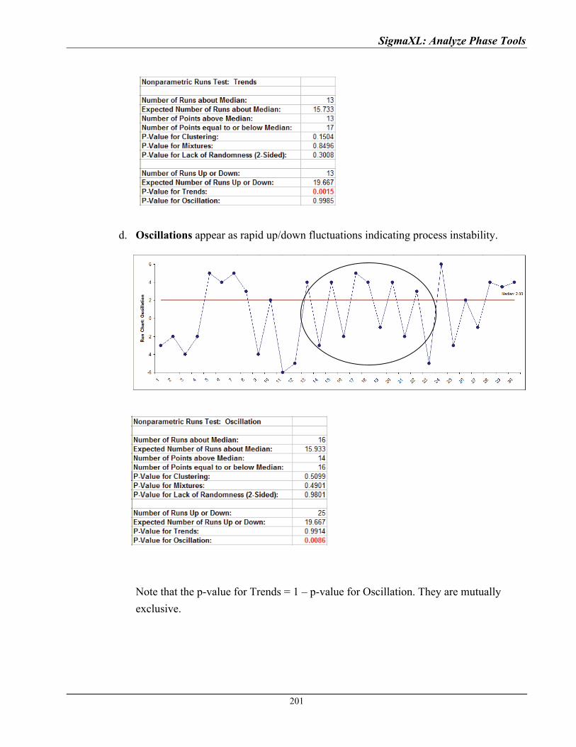
SigmaXL: Analyze Phase Tools
d. Oscillations appear as rapid up/down fluctuations indicating process instability.
Note that the p-value for Trends = 1 – p-value for Oscillation. They are mutually
exclusive.
201
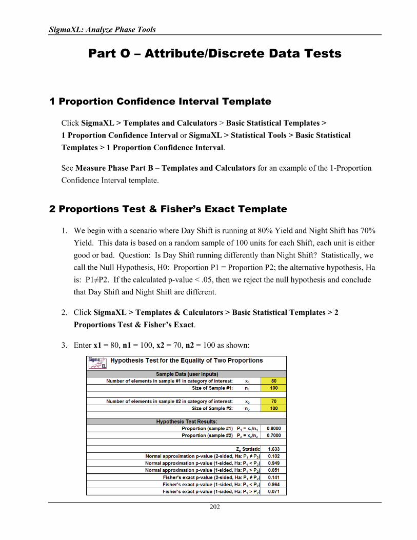
SigmaXL: Analyze Phase Tools
Part O – Attribute/Discrete Data Tests
1 Proportion Confidence Interval Template
Click SigmaXL > Templates and Calculators > Basic Statistical Templates >
1 Proportion Confidence Interval or SigmaXL > Statistical Tools > Basic Statistical
Templates > 1 Proportion Confidence Interval.
See Measure Phase Part B – Templates and Calculators for an example of the 1-Proportion
Confidence Interval template.
2 Proportions Test & Fisher’s Exact Template
1. We begin with a scenario where Day Shift is running at 80% Yield and Night Shift has 70%
Yield. This data is based on a random sample of 100 units for each Shift, each unit is either
good or bad. Question: Is Day Shift running differently than Night Shift? Statistically, we
call the Null Hypothesis, H0: Proportion P1 = Proportion P2; the alternative hypothesis, Ha
is: P1≠P2. If the calculated p-value < .05, then we reject the null hypothesis and conclude
that Day Shift and Night Shift are different.
2. Click SigmaXL > Templates & Calculators > Basic Statistical Templates > 2
Proportions Test & Fisher’s Exact.
3. Enter x1 = 80, n1 = 100, x2 = 70, n2 = 100 as shown:
202
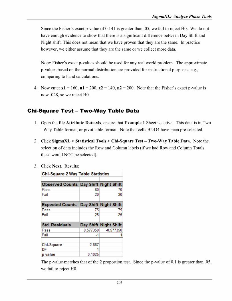
SigmaXL: Analyze Phase Tools
Since the Fisher’s exact p-value of 0.141 is greater than .05, we fail to reject H0. We do not
have enough evidence to show that there is a significant difference between Day Shift and
Night shift. This does not mean that we have proven that they are the same. In practice
however, we either assume that they are the same or we collect more data.
Note: Fisher’s exact p-values should be used for any real world problem. The approximate
p-values based on the normal distribution are provided for instructional purposes, e.g.,
comparing to hand calculations.
4. Now enter x1 = 160, n1 = 200, x2 = 140, n2 = 200. Note that the Fisher’s exact p-value is
now .028, so we reject H0.
Chi-Square Test – Two-Way Table Data
1. Open the file Attribute Data.xls, ensure that Example 1 Sheet is active. This data is in Two
–Way Table format, or pivot table format. Note that cells B2:D4 have been pre-selected.
2. Click SigmaXL > Statistical Tools > Chi-Square Test – Two-Way Table Data. Note the
selection of data includes the Row and Column labels (if we had Row and Column Totals
these would NOT be selected).
3. Click Next. Results:
The p-value matches that of the 2 proportion test. Since the p-value of 0.1 is greater than .05,
we fail to reject H0.
203
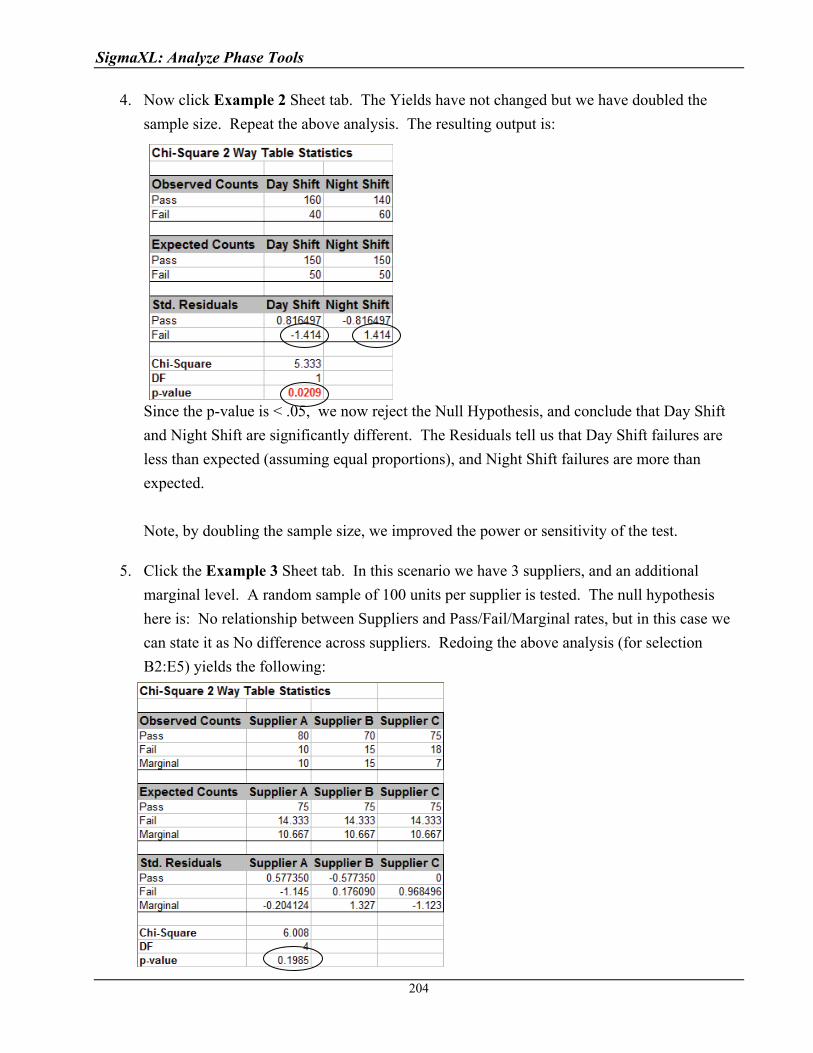
SigmaXL: Analyze Phase Tools
4. Now click Example 2 Sheet tab. The Yields have not changed but we have doubled the
sample size. Repeat the above analysis. The resulting output is:
Since the p-value is < .05, we now reject the Null Hypothesis, and conclude that Day Shift
and Night Shift are significantly different. The Residuals tell us that Day Shift failures are
less than expected (assuming equal proportions), and Night Shift failures are more than
expected.
Note, by doubling the sample size, we improved the power or sensitivity of the test.
5. Click the Example 3 Sheet tab. In this scenario we have 3 suppliers, and an additional
marginal level. A random sample of 100 units per supplier is tested. The null hypothesis
here is: No relationship between Suppliers and Pass/Fail/Marginal rates, but in this case we
can state it as No difference across suppliers. Redoing the above analysis (for selection
B2:E5) yields the following:
204

SigmaXL: Analyze Phase Tools
The p-value tells us that we do not have enough evidence to show that there is a difference
across the 3 suppliers.
6. Click the Example 4 Sheet tab. Here we have doubled the sample size to 200 per supplier.
Note that the percentages are identical to example 3. Redoing the above analysis yields the
following:
With the p-value < .05 we now conclude that there is a significant difference across
suppliers. Examining the residuals tells us that Supplier A has fewer failures than expected
(if there was no difference across suppliers) and Supplier C has more failures than expected.
Supplier B has more marginal parts than expected and Supplier C has fewer marginal parts
than expected.
205
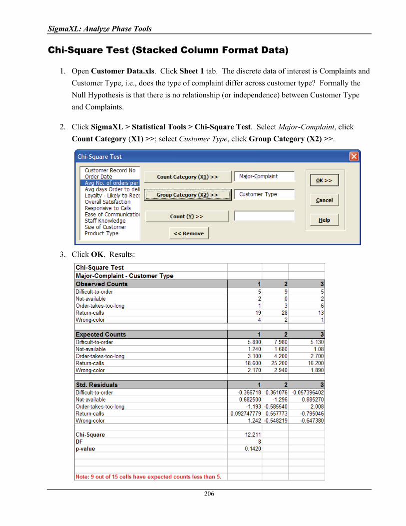
SigmaXL: Analyze Phase Tools
Chi-Square Test (Stacked Column Format Data)
1. Open Customer Data.xls. Click Sheet 1 tab. The discrete data of interest is Complaints and
Customer Type, i.e., does the type of complaint differ across customer type? Formally the
Null Hypothesis is that there is no relationship (or independence) between Customer Type
and Complaints.
2. Click SigmaXL > Statistical Tools > Chi-Square Test. Select Major-Complaint, click
Count Category (X1) >>; select Customer Type, click Group Category (X2) >>.
3. Click OK. Results:
206
SigmaXL: Analyze Phase Tools
207
With the p-value = 0.142 we fail to reject H0, so we do not have enough evidence to show a
difference in customer complaints across customer types.
Note: If more than 20% of Fitted Cells are Sparse - cells whose expected value is less than 5
– consider collecting more data, consolidation of levels, or removal of columns.
Tip: Use Chi-Square Analysis to complement Advanced Pareto Analysis.

SigmaXL: Analyze Phase Tools
Power & Sample Size for One Proportion Test
To determine Power & Sample Size for a 1 Proportion Test, you can use the Power & Sample
Size Calculator or Power & Sample Size with Worksheet.
1. Click SigmaXL > Statistical Tools > Power & Sample Size Calculators > 1 Proportion
Test Calculator.
2. Select Solve For Power (1 – Beta). Enter Sample Size and Alternative Proportion as
shown:
Note that we are calculating the power or likelihood of detection given that the hypothesized
proportion is 0.5, but the alternative proportion is 0.6, sample size = 300, significance level =
.05, and Ha: Not Equal To (two sided test).
3. Click OK. The resulting report is displayed:
A power value of 0.94 is acceptable, but note that the sample size n = 300, and the difference
208
SigmaXL: Analyze Phase Tools
209
in proportion value is 0.1 or 10%! The sample size requirements for discrete data are much
higher than those for continuous data.
4. To determine Power & Sample Size using a Worksheet, click SigmaXL > Statistical Tools
> Power & Sample Size with Worksheet > 1 Proportion Test.
5. A graph showing the relationship between Power, Sample Size and Proportion Value can
then be created using SigmaXL > Statistical Tools > Power & Sample Size Chart. See
Part E for an example using the 1 Sample t-Test.
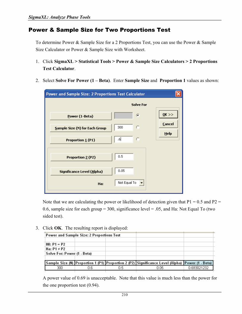
SigmaXL: Analyze Phase Tools
Power & Sample Size for Two Proportions Test
To determine Power & Sample Size for a 2 Proportions Test, you can use the Power & Sample
Size Calculator or Power & Sample Size with Worksheet.
1. Click SigmaXL > Statistical Tools > Power & Sample Size Calculators > 2 Proportions
Test Calculator.
2. Select Solve For Power (1 – Beta). Enter Sample Size and Proportion 1 values as shown:
Note that we are calculating the power or likelihood of detection given that P1 = 0.5 and P2 =
0.6, sample size for each group = 300, significance level = .05, and Ha: Not Equal To (two
sided test).
3. Click OK. The resulting report is displayed:
A power value of 0.69 is unacceptable. Note that this value is much less than the power for
the one proportion test (0.94).
210

SigmaXL: Analyze Phase Tools
211
4. To compensate, we will double the sample size per group. Press F3 or click Recall
SigmaXL Dialog to recall last dialog. Change the sample size per group from 300 to 600.
Note that the power value is now 0.94.
5. To determine Power & Sample Size using a Worksheet, click SigmaXL > Statistical Tools
> Power & Sample Size with Worksheet > 2 Proportions Test.
6. A graph showing the relationship between Power, Sample Size and Proportion Values can
then be created using SigmaXL > Statistical Tools > Power & Sample Size Chart. See
Part E for an example using the 1 Sample t-Test.
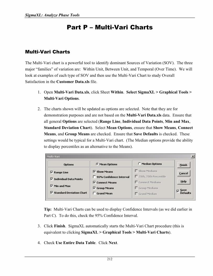
SigmaXL: Analyze Phase Tools
Part P – Multi-Vari Charts
Multi-Vari Charts
The Multi-Vari chart is a powerful tool to identify dominant Sources of Variation (SOV). The three
major “families” of variation are: Within Unit, Between Unit, and Temporal (Over Time). We will
look at examples of each type of SOV and then use the Multi-Vari Chart to study Overall
Satisfaction in the Customer Data.xls file.
1. Open Multi-Vari Data.xls, click Sheet Within. Select SigmaXL > Graphical Tools >
Multi-Vari Options.
2. The charts shown will be updated as options are selected. Note that they are for
demonstration purposes and are not based on the Multi-Vari Data.xls data. Ensure that
all general Options are selected (Range Line, Individual Data Points, Min and Max,
Standard Deviation Chart). Select Mean Options, ensure that Show Means, Connect
Means, and Group Means are checked. Ensure that Save Defaults is checked. These
settings would be typical for a Multi-Vari chart. (The Median options provide the ability
to display percentiles as an alternative to the Means).
Tip: Multi-Vari Charts can be used to display Confidence Intervals (as we did earlier in
Part C). To do this, check the 95% Confidence Interval.
3. Click Finish. SigmaXL automatically starts the Multi-Vari Chart procedure (this is
equivalent to clicking SigmaXL > Graphical Tools > Multi-Vari Charts).
4. Check Use Entire Data Table. Click Next.
212
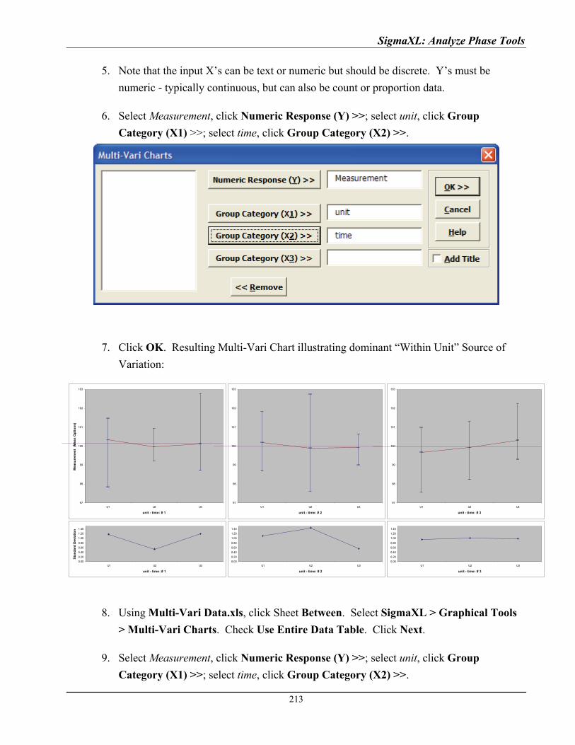
SigmaXL: Analyze Phase Tools
5. Note that the input X’s can be text or numeric but should be discrete. Y’s must be
numeric - typically continuous, but can also be count or proportion data.
6. Select Measurement, click Numeric Response (Y) >>; select unit, click Group
Category (X1) >>; select time, click Group Category (X2) >>.
7. Click OK. Resulting Multi-Vari Chart illustrating dominant “Within Unit” Source of
Variation:
97
98
99
100
101
102
103
U1 U2 U3
unit - time: # 1
Mea
sure
men
t (
Mea
n O
pti
on
s)
0.00
0.20
0.40
0.60
0.80
1.00
1.20
1.40
U1 U2 U3
unit - time: # 1
Sta
nd
ard
Dev
iati
on
97
98
99
100
101
102
103
U1 U2 U3
unit - time: # 2
0.00
0.20
0.40
0.60
0.80
1.00
1.20
1.40
U1 U2 U3
unit - time: # 2
97
98
99
100
101
102
103
U1 U2 U3
unit - time: # 3
0.00
0.20
0.40
0.60
0.80
1.00
1.20
1.40
U1 U2 U3
unit - time: # 3
8. Using Multi-Vari Data.xls, click Sheet Between. Select SigmaXL > Graphical Tools
> Multi-Vari Charts. Check Use Entire Data Table. Click Next.
9. Select Measurement, click Numeric Response (Y) >>; select unit, click Group
Category (X1) >>; select time, click Group Category (X2) >>.
213
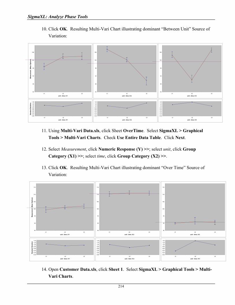
SigmaXL: Analyze Phase Tools
10. Click OK. Resulting Multi-Vari Chart illustrating dominant “Between Unit” Source of
Variation:
83
88
93
98
103
108
U1 U2 U3
unit - time: # 1
Mea
sure
men
t (
Mea
n O
pti
on
s)
0.00
0.20
0.40
0.60
0.80
1.00
1.20
1.40
U1 U2 U3
unit - time: # 1
Sta
nd
ard
Dev
iati
on
83
88
93
98
103
108
U1 U2 U3
unit - time: # 2
0.00
0.20
0.40
0.60
0.80
1.00
1.20
1.40
U1 U2 U3
unit - time: # 2
83
88
93
98
103
108
U1 U2 U3
unit - time: # 3
0.00
0.20
0.40
0.60
0.80
1.00
1.20
1.40
U1 U2 U3
unit - time: # 3
11. Using Multi-Vari Data.xls, click Sheet OverTime. Select SigmaXL > Graphical
Tools > Multi-Vari Charts. Check Use Entire Data Table. Click Next.
12. Select Measurement, click Numeric Response (Y) >>; select unit, click Group
Category (X1) >>; select time, click Group Category (X2) >>.
13. Click OK. Resulting Multi-Vari Chart illustrating dominant “Over Time” Source of
Variation:
.
85
90
95
100
105
110
115
U1 U2 U3
unit - time: # 1
Mea
sure
men
t (
Mea
n O
pti
on
s)
0.00
0.20
0.40
0.60
0.80
1.00
1.20
1.40
U1 U2 U3
unit - time: # 1
Sta
nd
ard
Dev
iati
on
85
90
95
100
105
110
115
U1 U2 U3
unit - time: # 2
0.00
0.20
0.40
0.60
0.80
1.00
1.20
1.40
U1 U2 U3
unit - time: # 2
85
90
95
100
105
110
115
U1 U2 U3
unit - time: # 3
0.00
0.20
0.40
0.60
0.80
1.00
1.20
1.40
U1 U2 U3
unit - time: # 3
14. Open Customer Data.xls, click Sheet 1. Select SigmaXL > Graphical Tools > Multi-
Vari Charts.
214
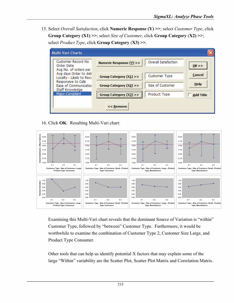
SigmaXL: Analyze Phase Tools
15. Select Overall Satisfaction, click Numeric Response (Y) >>; select Customer Type, click
Group Category (X1) >>; select Size of Customer, click Group Category (X2) >>;
select Product Type, click Group Category (X3) >>.
16. Click OK. Resulting Multi-Vari chart:
Examining this Multi-Vari chart reveals that the dominant Source of Variation is “within”
Customer Type, followed by “between” Customer Type. Furthermore, it would be
worthwhile to examine the combination of Customer Type 2, Customer Size Large, and
Product Type Consumer.
Other tools that can help us identify potential X factors that may explain some of the
large “Within” variability are the Scatter Plot, Scatter Plot Matrix and Correlation Matrix.
1.634
2.134
2.634
3.134
3.634
4.134
4.634
# 1 # 2 # 3
Customer Type - Size of Customer: Large - Product Type: Consumer
Ove
rall
Sat
isfa
ctio
n (
Mea
n O
pti
on
s)
0.00
0.20
0.40
0.60
0.80
1.00
# 1 # 2 # 3
Customer Type - Size of Customer: Large - Product Type: Consumer
Sta
nd
ard
Dev
iati
on
1.634
2.134
2.634
3.134
3.634
4.134
4.634
# 1 # 2 # 3
Customer Type - Size of Customer: Small - Product Type: Consumer
0.00
0.20
0.40
0.60
0.80
1.00
# 1 # 2 # 3
Customer Type - Size of Customer: Small - Product Type: Consumer
1.634
2.134
2.634
3.134
3.634
4.134
4.634
# 1 # 2 # 3
Customer Type - Size of Customer: Large - Product Type: Manufacturer
0.00
0.20
0.40
0.60
0.80
1.00
# 1 # 2 # 3
Customer Type - Size of Customer: Large - Product Type: Manufacturer
1.634
2.134
2.634
3.134
3.634
4.134
4.634
# 1 # 2 # 3
Customer Type - Size of Customer: Small - Product Type: Manufacturer
0.00
0.20
0.40
0.60
0.80
1.00
# 1 # 2 # 3
Customer Type - Size of Customer: Small - Product Type: Manufacturer
215
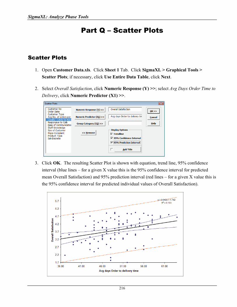
SigmaXL: Analyze Phase Tools
Part Q – Scatter Plots
Scatter Plots
1. Open Customer Data.xls. Click Sheet 1 Tab. Click SigmaXL > Graphical Tools >
Scatter Plots; if necessary, click Use Entire Data Table, click Next.
2. Select Overall Satisfaction, click Numeric Response (Y) >>; select Avg Days Order Time to
Delivery, click Numeric Predictor (X1) >>.
3. Click OK. The resulting Scatter Plot is shown with equation, trend line, 95% confidence
interval (blue lines – for a given X value this is the 95% confidence interval for predicted
mean Overall Satisfaction) and 95% prediction interval (red lines – for a given X value this is
the 95% confidence interval for predicted individual values of Overall Satisfaction).
216
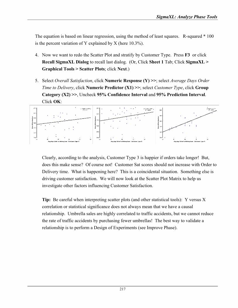
SigmaXL: Analyze Phase Tools
The equation is based on linear regression, using the method of least squares. R-squared * 100
is the percent variation of Y explained by X (here 10.3%).
4. Now we want to redo the Scatter Plot and stratify by Customer Type. Press F3 or click
Recall SigmaXL Dialog to recall last dialog. (Or, Click Sheet 1 Tab; Click SigmaXL >
Graphical Tools > Scatter Plots; click Next.)
5. Select Overall Satisfaction, click Numeric Response (Y) >>; select Average Days Order
Time to Delivery, click Numeric Predictor (X1) >>; select Customer Type, click Group
Category (X2) >>, Uncheck 95% Confidence Interval and 95% Prediction Interval.
Click OK:
Clearly, according to the analysis, Customer Type 3 is happier if orders take longer! But,
does this make sense? Of course not! Customer Sat scores should not increase with Order to
Delivery time. What is happening here? This is a coincidental situation. Something else is
driving customer satisfaction. We will now look at the Scatter Plot Matrix to help us
investigate other factors influencing Customer Satisfaction.
Tip: Be careful when interpreting scatter plots (and other statistical tools): Y versus X
correlation or statistical significance does not always mean that we have a causal
relationship. Umbrella sales are highly correlated to traffic accidents, but we cannot reduce
the rate of traffic accidents by purchasing fewer umbrellas! The best way to validate a
relationship is to perform a Design of Experiments (see Improve Phase).
217
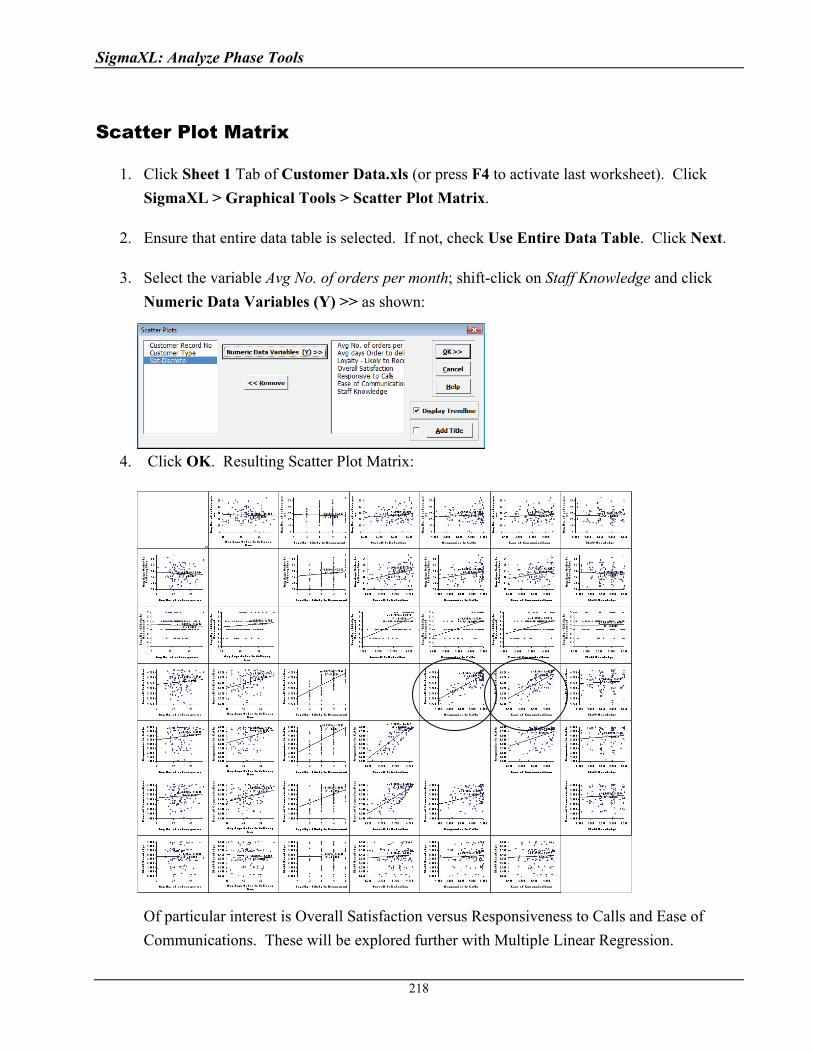
SigmaXL: Analyze Phase Tools
Scatter Plot Matrix
1. Click Sheet 1 Tab of Customer Data.xls (or press F4 to activate last worksheet). Click
SigmaXL > Graphical Tools > Scatter Plot Matrix.
2. Ensure that entire data table is selected. If not, check Use Entire Data Table. Click Next.
3. Select the variable Avg No. of orders per month; shift-click on Staff Knowledge and click
Numeric Data Variables (Y) >> as shown:
4. Click OK. Resulting Scatter Plot Matrix:
Of particular interest is Overall Satisfaction versus Responsiveness to Calls and Ease of
Communications. These will be explored further with Multiple Linear Regression.
218

SigmaXL: Analyze Phase Tools
Part R – Correlation Matrix
The correlation matrix complements the scatterplot matrix by quantifying the degree of association.
The following table shows the approximate relationship between r, R-squared, and degree of
association:
Pearson Correlation Coefficient
(r)
R-Squared (%) Degree of association
0.9 <= |r| <=1 > 80 % Strong
0.7 <= |r| < 0.9 50 % to 80 % Moderate
|r| < 0.7 < 50 % Weak
Pearson Probability, p > 0.05 None
Correlation Matrix
1. Open Customer Data.xls. Click Sheet 1 tab (or press F4 to activate last worksheet). Click
SigmaXL > Statistical Tools > Correlation Matrix. Ensure that entire data table is selected. If
not, check Use Entire Data Table. Click Next.
2. Select the variable Avg No. of orders per month; shift-click on Staff Knowledge and click
Numeric Data Variables (Y) >> as shown:
219
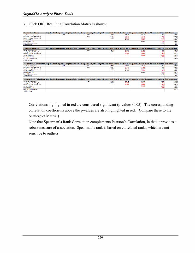
SigmaXL: Analyze Phase Tools
3. Click OK. Resulting Correlation Matrix is shown:
Correlations highlighted in red are considered significant (p-values < .05). The corresponding
correlation coefficients above the p-values are also highlighted in red. (Compare these to the
Scatterplot Matrix.)
Note that Spearman’s Rank Correlation complements Pearson’s Correlation, in that it provides a
robust measure of association. Spearman’s rank is based on correlated ranks, which are not
sensitive to outliers.
220
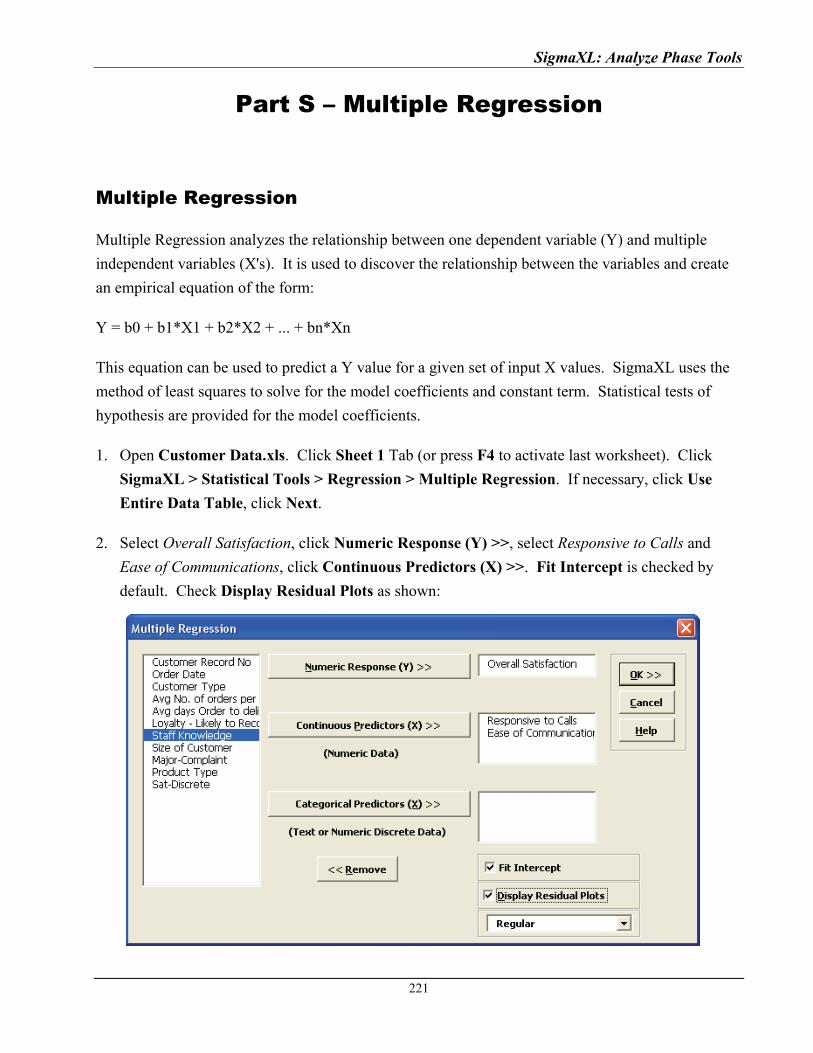
SigmaXL: Analyze Phase Tools
Part S – Multiple Regression
Multiple Regression
Multiple Regression analyzes the relationship between one dependent variable (Y) and multiple
independent variables (X's). It is used to discover the relationship between the variables and create
an empirical equation of the form:
Y = b0 + b1*X1 + b2*X2 + ... + bn*Xn
This equation can be used to predict a Y value for a given set of input X values. SigmaXL uses the
method of least squares to solve for the model coefficients and constant term. Statistical tests of
hypothesis are provided for the model coefficients.
1. Open Customer Data.xls. Click Sheet 1 Tab (or press F4 to activate last worksheet). Click
SigmaXL > Statistical Tools > Regression > Multiple Regression. If necessary, click Use
Entire Data Table, click Next.
2. Select Overall Satisfaction, click Numeric Response (Y) >>, select Responsive to Calls and
Ease of Communications, click Continuous Predictors (X) >>. Fit Intercept is checked by
default. Check Display Residual Plots as shown:
221
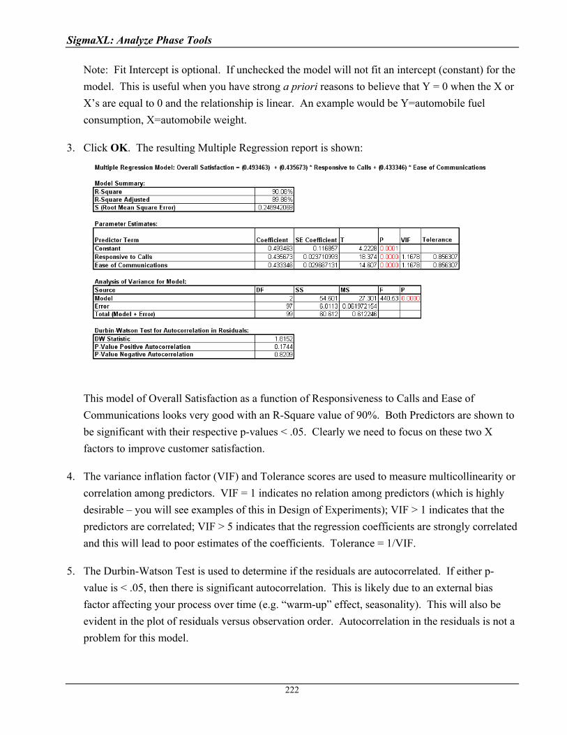
SigmaXL: Analyze Phase Tools
Note: Fit Intercept is optional. If unchecked the model will not fit an intercept (constant) for the
model. This is useful when you have strong a priori reasons to believe that Y = 0 when the X or
X’s are equal to 0 and the relationship is linear. An example would be Y=automobile fuel
consumption, X=automobile weight.
3. Click OK. The resulting Multiple Regression report is shown:
This model of Overall Satisfaction as a function of Responsiveness to Calls and Ease of
Communications looks very good with an R-Square value of 90%. Both Predictors are shown to
be significant with their respective p-values < .05. Clearly we need to focus on these two X
factors to improve customer satisfaction.
4. The variance inflation factor (VIF) and Tolerance scores are used to measure multicollinearity or
correlation among predictors. VIF = 1 indicates no relation among predictors (which is highly
desirable – you will see examples of this in Design of Experiments); VIF > 1 indicates that the
predictors are correlated; VIF > 5 indicates that the regression coefficients are strongly correlated
and this will lead to poor estimates of the coefficients. Tolerance = 1/VIF.
5. The Durbin-Watson Test is used to determine if the residuals are autocorrelated. If either p-
value is < .05, then there is significant autocorrelation. This is likely due to an external bias
factor affecting your process over time (e.g. “warm-up” effect, seasonality). This will also be
evident in the plot of residuals versus observation order. Autocorrelation in the residuals is not a
problem for this model.
222
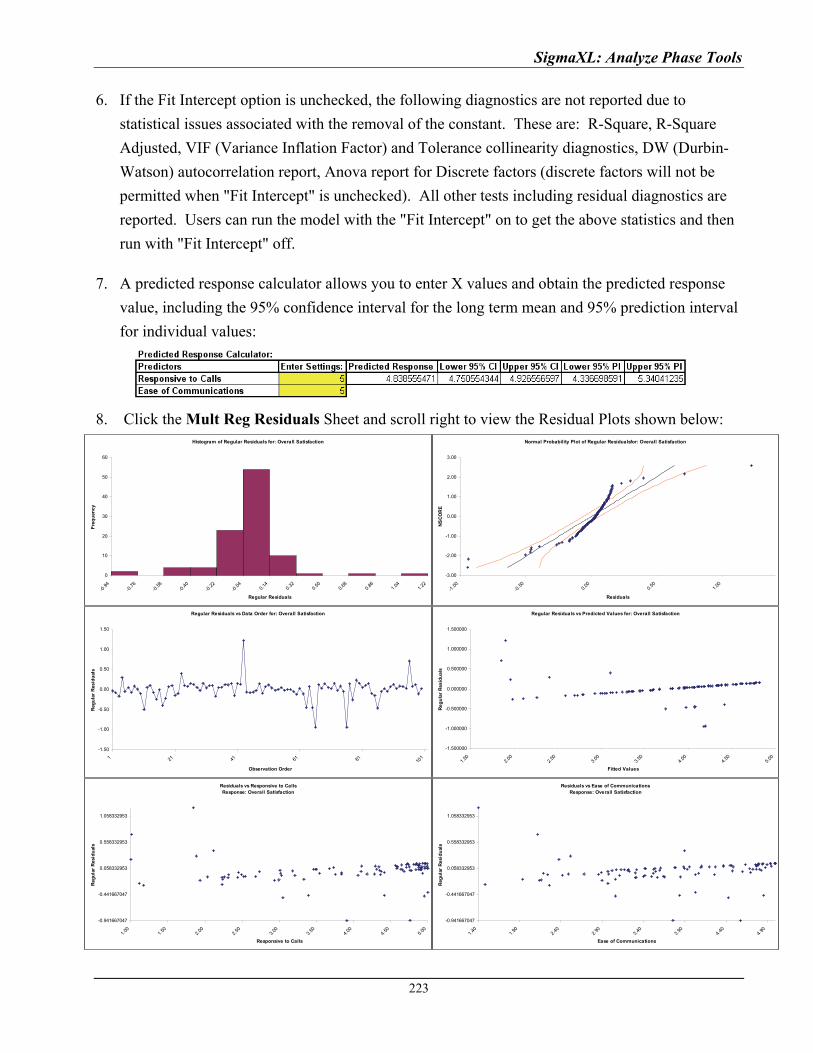
SigmaXL: Analyze Phase Tools
6. If the Fit Intercept option is unchecked, the following diagnostics are not reported due to
statistical issues associated with the removal of the constant. These are: R-Square, R-Square
Adjusted, VIF (Variance Inflation Factor) and Tolerance collinearity diagnostics, DW (Durbin-
Watson) autocorrelation report, Anova report for Discrete factors (discrete factors will not be
permitted when "Fit Intercept" is unchecked). All other tests including residual diagnostics are
reported. Users can run the model with the "Fit Intercept" on to get the above statistics and then
run with "Fit Intercept" off.
7. A predicted response calculator allows you to enter X values and obtain the predicted response
value, including the 95% confidence interval for the long term mean and 95% prediction interval
for individual values:
8. Click the Mult Reg Residuals Sheet and scroll right to view the Residual Plots shown below:
Histogram of Regular Residuals for: Overall Satisfaction
0
10
20
30
40
50
60
-0.94
-0.76
-0.58
-0.40
-0.22
-0.04 0.
140.
320.
500.
680.
861.
041.
22
Regular Residuals
Fre
qu
ency
Normal Probability Plot of Regular Residualsfor: Overall Satisfaction
-3.00
-2.00
-1.00
0.00
1.00
2.00
3.00
-1.00
-0.50 0.
000.
501.
00
Residuals
NS
CO
RE
Regular Residuals vs Predicted Values for: Overall Satisfaction
-1.500000
-1.000000
-0.500000
0.000000
0.500000
1.000000
1.500000
1.50
2.00
2.50
3.00
3.50
4.00
4.50
5.00
Fitted Values
Reg
ula
r R
esid
ual
s
Regular Residuals vs Data Order for: Overall Satisfaction
-1.50
-1.00
-0.50
0.00
0.50
1.00
1.50
1 21 41 61 81 101
Observation Order
Reg
ula
r R
esid
ual
s
Residuals vs Responsive to CallsResponse: Overall Satisfaction
-0.941667047
-0.441667047
0.058332953
0.558332953
1.058332953
1.00
1.50
2.00
2.50
3.00
3.50
4.00
4.50
5.00
Responsive to Calls
Reg
ula
r R
esid
ual
s
Residuals vs Ease of CommunicationsResponse: Overall Satisfaction
-0.941667047
-0.441667047
0.058332953
0.558332953
1.058332953
1.40
1.90
2.40
2.90
3.40
3.90
4.40
4.90
Ease of Communications
Reg
ula
r R
esid
ual
s
223

SigmaXL: Analyze Phase Tools
Residuals are the unexplained variation from the regression model (Y - Ŷ). We expect to see the
residuals normally distributed with no obvious patterns in the above graphs. Clearly this is not
the case here, with the Residuals versus Predicted Values indicating there is likely some other X
factor influencing the Overall Satisfaction. It would be appropriate to consider other factors in
the model.
9. SigmaXL also provides Standardized Residuals and Studentized (Deleted t) Residuals. The
standardized residual is the residual, divided by an estimate of its standard deviation. This makes
it easier to detect outliers. Standardized residuals greater than 3 and less than -3 are considered
large (these outliers are highlighted in red). Studentized deleted residuals are computed in the
same way that standardized residuals are computed, except that the ith observation is removed
before performing the regression fit. This prevents the ith observation from influencing the
regression model, resulting in unusual observations being more likely to stand out.
10. Click Recall Last Dialog (or press F3). Change the Residual type to Standardized. Click OK.
The resulting Standardized Residual plots are displayed:
Histogram of Standardized Residuals for: Overall Satisfaction
0
10
20
30
40
50
60
70
-3.82
-3.07
-2.33
-1.58
-0.84
-0.09 0.
651.
402.
142.
893.
634.
385.
12
Standardized Residuals
Fre
qu
ency
Normal Probability Plot of Standardized Residuals for: Overall Satisfaction
-3.00
-2.00
-1.00
0.00
1.00
2.00
3.00
-4.00
0
-3.00
0
-2.00
0
-1.00
0
0.00
01.
000
2.00
03.
000
4.00
05.
000
6.00
0
Standardized Residuals
NS
CO
RE
Standardized Residuals vs Predicted Values for: Overall Satisfaction
-5.000
-4.000
-3.000
-2.000
-1.000
0.000
1.000
2.000
3.000
4.000
5.000
6.000
1.50
2.00
2.50
3.00
3.50
4.00
4.50
5.00
Fitted Values
Sta
nd
ard
ized
Res
idu
als
Standardized Residuals vs Data Order for: Overall Satisfaction
-5.00
-4.00
-3.00
-2.00
-1.00
0.00
1.00
2.00
3.00
4.00
5.00
6.00
1 21 41 61 81 101
Observation Order
Sta
nd
ard
ized
Res
idu
als
Residuals vs Responsive to CallsResponse: Overall Satisfaction
-3.820146
-2.820146
-1.820146
-0.820146
0.179854
1.179854
2.179854
3.179854
4.179854
224
1.0
anrd
ds
01.
502.
002.
503.
003.
504.
004.
505.
00
Responsive to Calls
St
da
ized
Res
iu
al
Residuals vs Ease of CommunicationsResponse: Overall Satisfaction
-3.820146
-2.820146
-1.820146
-0.820146
0.179854
1.179854
2.179854
3.179854
4.179854
1.40
1.90
2.40
2.90
3.40
3.90
4.40
4.90
Ease of Communications
Sta
nd
ard
ized
Res
idu
als
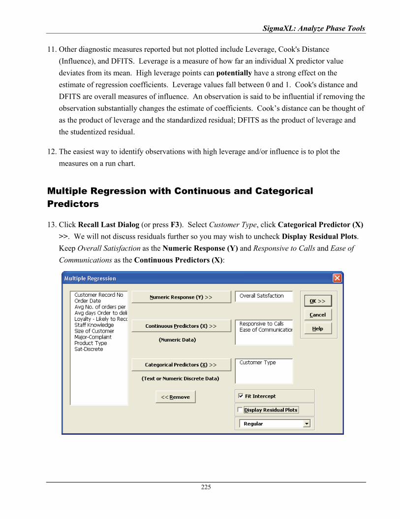
SigmaXL: Analyze Phase Tools
11. Other diagnostic measures reported but not plotted include Leverage, Cook's Distance
(Influence), and DFITS. Leverage is a measure of how far an individual X predictor value
deviates from its mean. High leverage points can potentially have a strong effect on the
estimate of regression coefficients. Leverage values fall between 0 and 1. Cook's distance and
DFITS are overall measures of influence. An observation is said to be influential if removing the
observation substantially changes the estimate of coefficients. Cook’s distance can be thought of
as the product of leverage and the standardized residual; DFITS as the product of leverage and
the studentized residual.
12. The easiest way to identify observations with high leverage and/or influence is to plot the
measures on a run chart.
Multiple Regression with Continuous and Categorical Predictors
13. Click Recall Last Dialog (or press F3). Select Customer Type, click Categorical Predictor (X)
>>. We will not discuss residuals further so you may wish to uncheck Display Residual Plots.
Keep Overall Satisfaction as the Numeric Response (Y) and Responsive to Calls and Ease of
Communications as the Continuous Predictors (X):
225
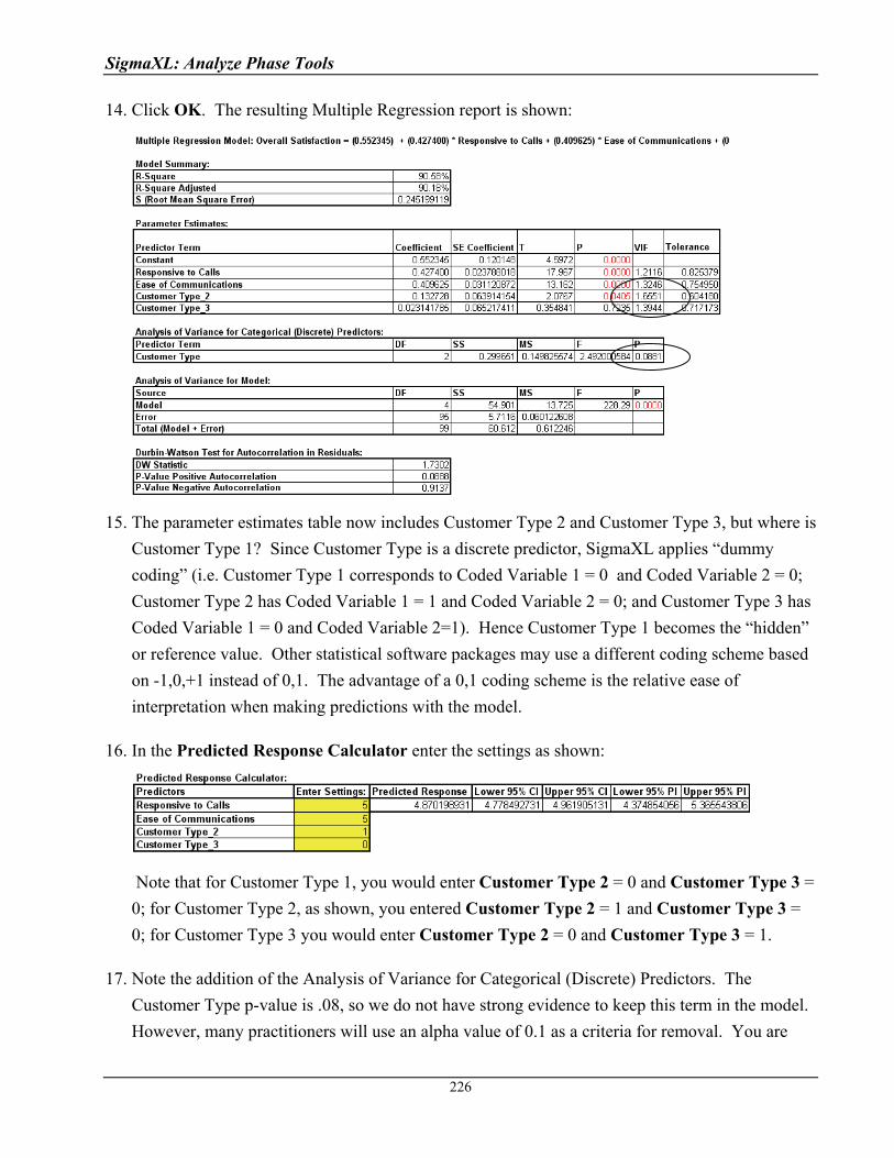
SigmaXL: Analyze Phase Tools
14. Click OK. The resulting Multiple Regression report is shown:
15. The parameter estimates table now includes Customer Type 2 and Customer Type 3, but where is
Customer Type 1? Since Customer Type is a discrete predictor, SigmaXL applies “dummy
coding” (i.e. Customer Type 1 corresponds to Coded Variable 1 = 0 and Coded Variable 2 = 0;
Customer Type 2 has Coded Variable 1 = 1 and Coded Variable 2 = 0; and Customer Type 3 has
Coded Variable 1 = 0 and Coded Variable 2=1). Hence Customer Type 1 becomes the “hidden”
or reference value. Other statistical software packages may use a different coding scheme based
on -1,0,+1 instead of 0,1. The advantage of a 0,1 coding scheme is the relative ease of
interpretation when making predictions with the model.
16. In the Predicted Response Calculator enter the settings as shown:
Note that for Customer Type 1, you would enter Customer Type 2 = 0 and Customer Type 3 =
0; for Customer Type 2, as shown, you entered Customer Type 2 = 1 and Customer Type 3 =
0; for Customer Type 3 you would enter Customer Type 2 = 0 and Customer Type 3 = 1.
17. Note the addition of the Analysis of Variance for Categorical (Discrete) Predictors. The
Customer Type p-value is .08, so we do not have strong evidence to keep this term in the model.
However, many practitioners will use an alpha value of 0.1 as a criteria for removal. You are
226

SigmaXL: Analyze Phase Tools
227
probably wondering why the p-value for Customer Type is not lower given the results we saw
earlier using ANOVA. The change in p-value is due to the inclusion of Responsive to Calls and
Ease of Communications in the model. We have higher scores for Ease of Communications and
Responsive to Calls with Customer Type 2. Statistically, Customer Type is somewhat correlated
to Responsive to Calls and Ease of Communications (VIF for Customer Type = 1.66 and 1.39).
SigmaXL: Analyze Phase Tools
228
Part T – Logistic Regression
Binary Logistic Regression
Binary Logistic Regression is used to analyze the relationship between one binary dependent
variable (Y) and multiple independent numeric and/or discrete variables (X's). It is used to discover
the relationship between the variables and create an empirical equation of the form:
Ln(Py/(1-Py)) = b0 + b1*X1 + b2*X2 + ... + bn*Xn
This equation can be used to predict an event probability Y value for a given set of input X values.
SigmaXL uses the method of maximum likelihood to solve for the model coefficients and constant
term. Statistical tests of hypothesis and odds-ratios are provided for the model coefficients. The
odds-ratios identify change in likelihood of the event for one unit change in X.
An example application from medical research would be Y=Disease (Yes/No) and X’s = Age,
Smoker (Yes/No), Number Years of Smoking and Weight. The model coefficient p-values would
indicate which X’s are significant and the odds-ratios would provide the relative change in risk for
each unit change in X.
We will analyze the familiar Customer Satisfaction data using Y=Discrete Satisfaction where the
values have been coded such that an Overall Satisfaction score >= 3.5 is considered a 1, and scores <
3.5 are considered a 0. Please note, we are not advising that continuous data be converted to discrete
data in actual practice, but simply using the Discrete Satisfaction score for continuity with the
previous analysis.
1. Open Customer Data.xls. Click Sheet 1 Tab (or press F4 to activate last worksheet). Click
SigmaXL > Statistical Tools > Regression > Binary Logistic Regression. If necessary, click
Use Entire Data Table, click Next.
2. Select Sat-Discrete, click Binary Response (Y) >>; select Responsive to Calls and Ease of
Communications, click Continuous Predictors (X) >>; select Customer Type, click Categorical
Predictors (X) >>.
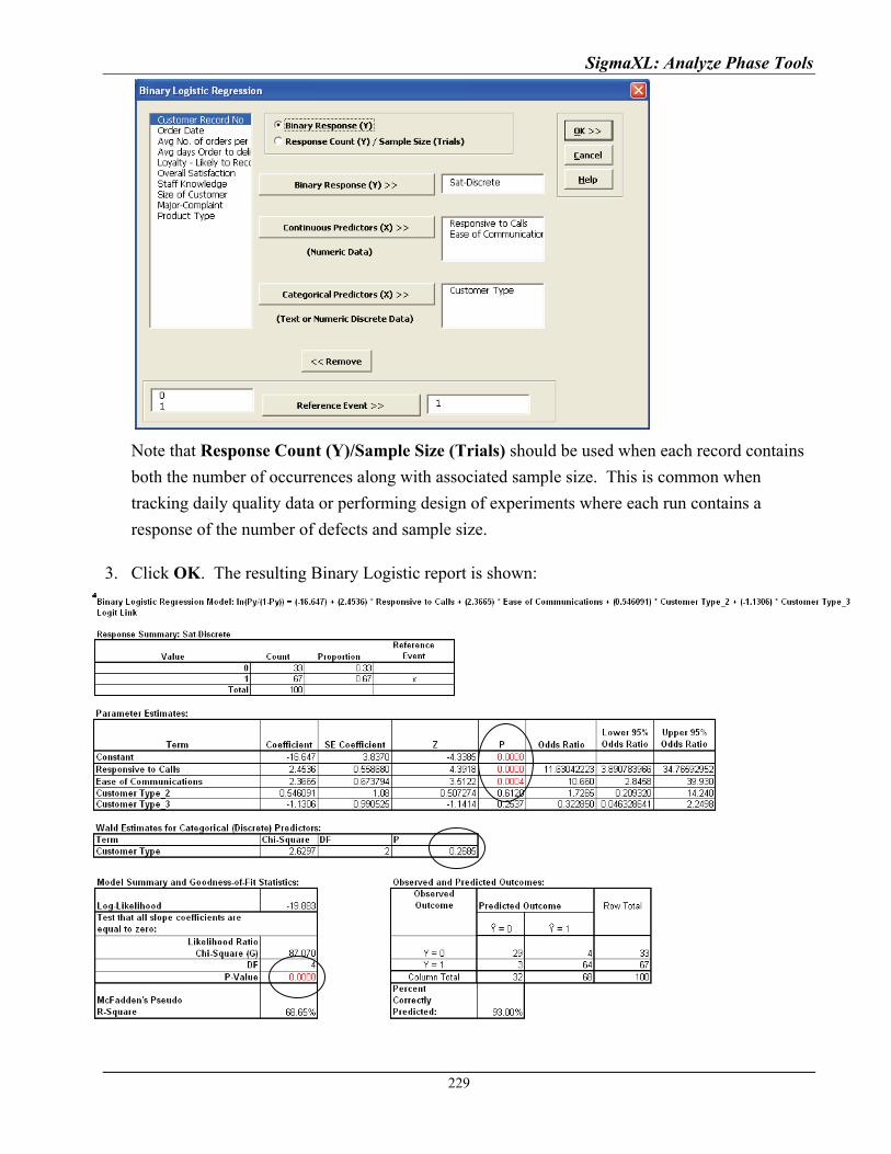
SigmaXL: Analyze Phase Tools
Note that Response Count (Y)/Sample Size (Trials) should be used when each record contains
both the number of occurrences along with associated sample size. This is common when
tracking daily quality data or performing design of experiments where each run contains a
response of the number of defects and sample size.
3. Click OK. The resulting Binary Logistic report is shown:
229

SigmaXL: Analyze Phase Tools
4. The Likelihood Ratio p-value < .05 tells us that the model is significant. The p-values for the
coefficients in the Parameter Estimates table confirm that Responsive to Calls and Ease of
Communications are significant.
5. The p-value in Wald Estimates for Categorical (Discrete) Predictors table tells us that Customer
Type is not significant here.
Tip: Significance for categorical predictors should be based on the Wald Estimates not the p-
values given in the Parameter Estimates table.
6. Note that Customer Type 1 is not displayed in the Parameter Estimates table. This is the
“hidden” reference value for Customer Type. Categorical predictors must have one level
selected as a reference value. SigmaXL sorts the levels alphanumerically and selects the first
level as the reference value.
7. Now we will rerun the binary logistic regression but remove Customer Type as a predictor. Press
F3 or click Recall SigmaXL Dialog to recall last dialog. Remove Customer Type by
highlighting Customer Type and double-clicking (or press the Remove button).
8. Click OK. The resulting Binary Logistic report is shown:
230
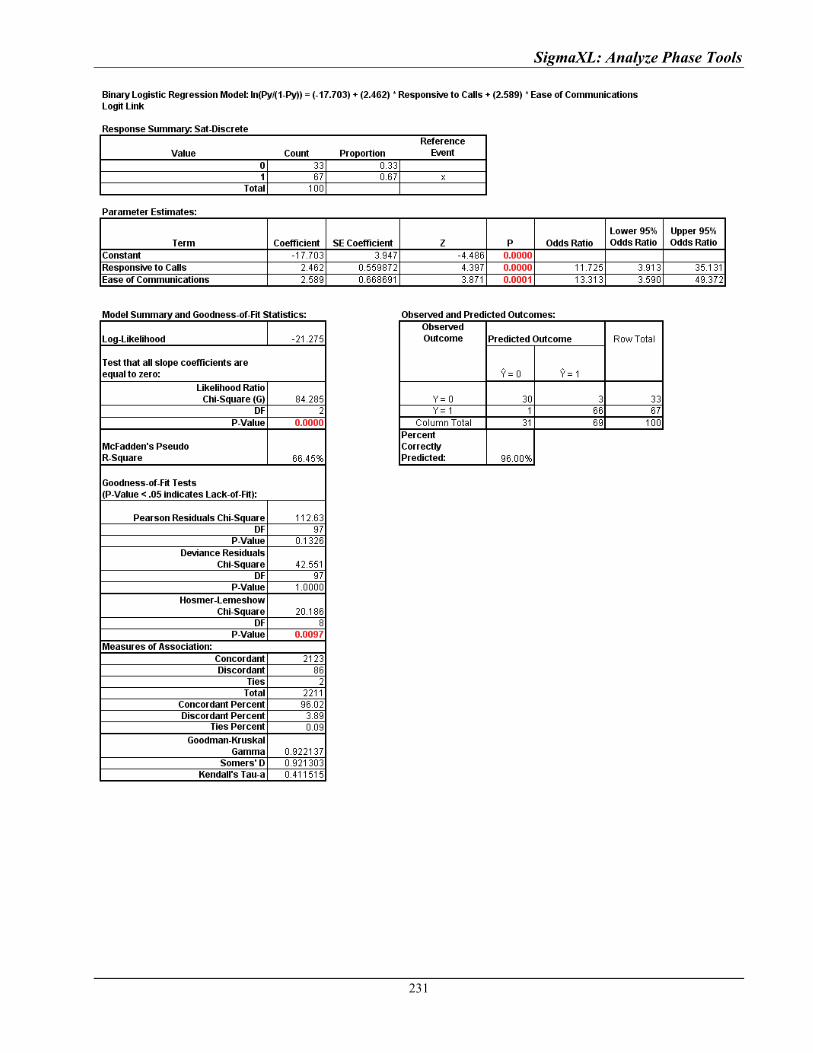
SigmaXL: Analyze Phase Tools
231
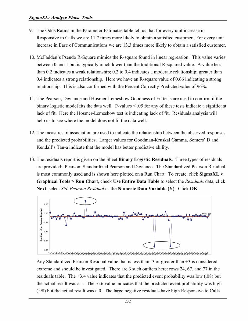
SigmaXL: Analyze Phase Tools
9. The Odds Ratios in the Parameter Estimates table tell us that for every unit increase in
Responsive to Calls we are 11.7 times more likely to obtain a satisfied customer. For every unit
increase in Ease of Communications we are 13.3 times more likely to obtain a satisfied customer.
10. McFadden’s Pseudo R-Square mimics the R-square found in linear regression. This value varies
between 0 and 1 but is typically much lower than the traditional R-squared value. A value less
than 0.2 indicates a weak relationship; 0.2 to 0.4 indicates a moderate relationship; greater than
0.4 indicates a strong relationship. Here we have an R-square value of 0.66 indicating a strong
relationship. This is also confirmed with the Percent Correctly Predicted value of 96%.
11. The Pearson, Deviance and Hosmer-Lemeshow Goodness of Fit tests are used to confirm if the
binary logistic model fits the data well. P-values < .05 for any of these tests indicate a significant
lack of fit. Here the Hosmer-Lemeshow test is indicating lack of fit. Residuals analysis will
help us to see where the model does not fit the data well.
12. The measures of association are used to indicate the relationship between the observed responses
and the predicted probabilities. Larger values for Goodman-Kruskal Gamma, Somers’ D and
Kendall’s Tau-a indicate that the model has better predictive ability.
13. The residuals report is given on the Sheet Binary Logistic Residuals. Three types of residuals
are provided: Pearson, Standardized Pearson and Deviance. The Standardized Pearson Residual
is most commonly used and is shown here plotted on a Run Chart. To create, click SigmaXL >
Graphical Tools > Run Chart, check Use Entire Data Table to select the Residuals data, click
Next, select Std. Pearson Residual as the Numeric Data Variable (Y). Click OK.
Any Standardized Pearson Residual value that is less than -3 or greater than +3 is considered
extreme and should be investigated. There are 3 such outliers here: rows 24, 67, and 77 in the
residuals table. The +3.4 value indicates that the predicted event probability was low (.08) but
the actual result was a 1. The -6.6 value indicates that the predicted event probability was high
(.98) but the actual result was a 0. The large negative residuals have high Responsive to Calls
Mean: -0.05
-7.34
-5.34
-3.34
-1.34
0.66
2.66
1 2 3 4 5 6 7 8 9101112131415161718192021222324252627282930313233343536373839404142434445464748495051525354555657585960616263646566676869707172737475767778798081828384858687888990919293949596979899100
Ru
n C
har
t -
Std
. P
ears
on
Res
idu
al
232
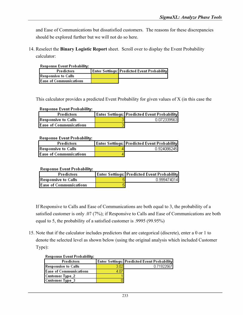
SigmaXL: Analyze Phase Tools
and Ease of Communications but dissatisfied customers. The reasons for these discrepancies
should be explored further but we will not do so here.
14. Reselect the Binary Logistic Report sheet. Scroll over to display the Event Probability
calculator:
This calculator provides a predicted Event Probability for given values of X (in this case the
probability of a satisfied customer). Enter the values 3,3; 4,4; 5,5 as shown:
If Responsive to Calls and Ease of Communications are both equal to 3, the probability of a
satisfied customer is only .07 (7%); if Responsive to Calls and Ease of Communications are both
equal to 5, the probability of a satisfied customer is .9995 (99.95%)
15. Note that if the calculator includes predictors that are categorical (discrete), enter a 0 or 1 to
denote the selected level as shown below (using the original analysis which included Customer
Type):
233

SigmaXL: Analyze Phase Tools
If we wanted to select Customer Type 1, enter a 0 for both Customer Types 2 and 3. Customer
Type 1 is the hidden reference value.
Ordinal Logistic Regression
Ordinal Logistic Regression is used to analyze the relationship between one ordinal dependent
variable (Y) and multiple independent continuous and/or discrete variables (X's).
We will analyze the Customer Satisfaction data using Y=Loyalty –Likely to Recommend score
which contains ordinal integer values from 1 to 5, where 5 indicates that the customer is very likely
to recommend us and 1 indicates that they are very likely to not recommend us.
1. Open Customer Data.xls. Click Sheet 1 Tab (or press F4 to activate last worksheet). Click
SigmaXL > Statistical Tools > Regression > Ordinal Logistic Regression. If necessary, click
Use Entire Data Table, click Next.
2. Select Loyalty – Likely to Recommend, click Numeric Ordinal Response (Y) >>; select
Responsive to Calls and Ease of Communications, click Continuous Predictors (X) >>.
3. Click OK. The resulting Ordinal Logistic report is shown:
234
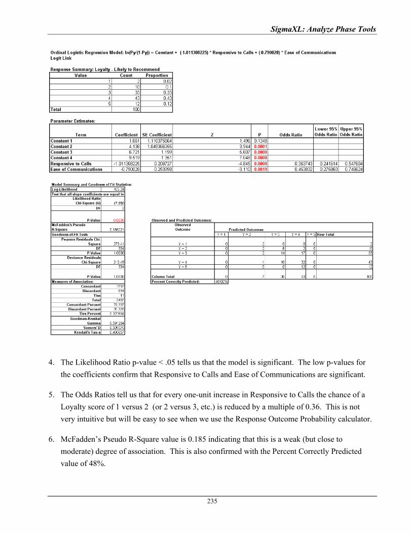
SigmaXL: Analyze Phase Tools
4. The Likelihood Ratio p-value < .05 tells us that the model is significant. The low p-values for
the coefficients confirm that Responsive to Calls and Ease of Communications are significant.
5. The Odds Ratios tell us that for every one-unit increase in Responsive to Calls the chance of a
Loyalty score of 1 versus 2 (or 2 versus 3, etc.) is reduced by a multiple of 0.36. This is not
very intuitive but will be easy to see when we use the Response Outcome Probability calculator.
6. McFadden’s Pseudo R-Square value is 0.185 indicating that this is a weak (but close to
moderate) degree of association. This is also confirmed with the Percent Correctly Predicted
value of 48%.
235

SigmaXL: Analyze Phase Tools
7. The Pearson and Deviance Goodness of Fit (GOF) tests are used to confirm if the ordinal logistic
model fits the data well. P-values < .05 would indicate a significant lack of fit. Given that the
GOF p-values are greater than .05, we conclude that there is no significant lack of fit.
8. Scroll across to the Response Outcome Probability calculator. This calculator provides predicted
outcome (event) probabilities for given values of X (in this case the probability of a satisfied
customer). Enter the values 3,3; 4,4; 5,5 as shown:
9. Referring to the Predicted Probability for each Level, if Responsive to Calls and Ease of
Communications are both equal to 3, we would expect to see typical loyalty scores of 3 (57%)
with some at 2 (20%) and 4 (20%); if Responsive to Calls and Ease of Communications are
both equal to 5, we would expect typical loyalty scores of 4 (53 %) with some at 3 (34%) and 5
(9%).
236

Copyright © 2004-2011, SigmaXL Inc.
SigmaXL: Improve Phase Tools: Design of Experiments (DOE)

SigmaXL: Improve Phase Tools: DOE
239
Part A – Overview of Basic Design of Experiments (DOE) Templates
The DOE templates are similar to the other SigmaXL templates: simply enter the inputs and
resulting outputs are produced immediately. The DOE templates provide common 2-level designs
for 2 to 5 factors. These basic templates are ideal for training, but use SigmaXL > Design of
Experiments > 2-Level Factorial/Screening Designs to accommodate up to 19 factors with
randomization, replication and blocking.
Click SigmaXL > Design of Experiments > Basic DOE Templates to access these templates:
Two-Factor, 4-Run, Full-Factorial
Three-Factor, 4-Run, Half-Fraction, Res III
Three-Factor, 8-Run, Full-Factorial
Four-Factor, 8-Run, Half-Fraction, Res IV
Four-Factor, 16-Run, Full-Factorial
Five-Factor, 8-Run, Quarter-Fraction, Res III
Five-Factor, 16-Run, Half-Fraction, Res V
After entering the template data, main effects and interaction plots may be created by clicking
SigmaXL > Basic DOE Templates > Main Effects & Interaction Plots. The DOE template must
be the active worksheet.
DOE Templates are protected worksheets by default, but this may be modified by clicking SigmaXL
> Help > Unprotect Worksheet.
Advanced analysis is available, but this requires that you unprotect the DOE worksheet. The
following example shows how to use Excel’s Equation Solver and SigmaXL’s Multiple Regression
in conjunction with a DOE template. Caution: If you unprotect the worksheet, do not change the
worksheet title (e.g. Three-Factor, Two-Level, 8-Run, Full-Factorial Design of Experiments).
This title is used by the Main Effects & Interaction Plots to determine appropriate analysis. Also, do
not modify any cells with formulas.
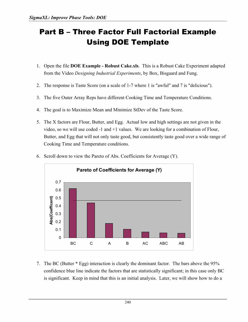
SigmaXL: Improve Phase Tools: DOE
Part B – Three Factor Full Factorial Example Using DOE Template
1. Open the file DOE Example - Robust Cake.xls. This is a Robust Cake Experiment adapted
from the Video Designing Industrial Experiments, by Box, Bisgaard and Fung.
2. The response is Taste Score (on a scale of 1-7 where 1 is "awful" and 7 is "delicious").
3. The five Outer Array Reps have different Cooking Time and Temperature Conditions.
4. The goal is to Maximize Mean and Minimize StDev of the Taste Score.
5. The X factors are Flour, Butter, and Egg. Actual low and high settings are not given in the
video, so we will use coded -1 and +1 values. We are looking for a combination of Flour,
Butter, and Egg that will not only taste good, but consistently taste good over a wide range of
Cooking Time and Temperature conditions.
6. Scroll down to view the Pareto of Abs. Coefficients for Average (Y).
Pareto of Coefficients for Average (Y)
0
0.1
0.2
0.3
0.4
0.5
0.6
0.7
BC C A B AC ABC AB
Ab
s(C
oef
fice
nt)
7. The BC (Butter * Egg) interaction is clearly the dominant factor. The bars above the 95%
confidence blue line indicate the factors that are statistically significant; in this case only BC
is significant. Keep in mind that this is an initial analysis. Later, we will show how to do a
240
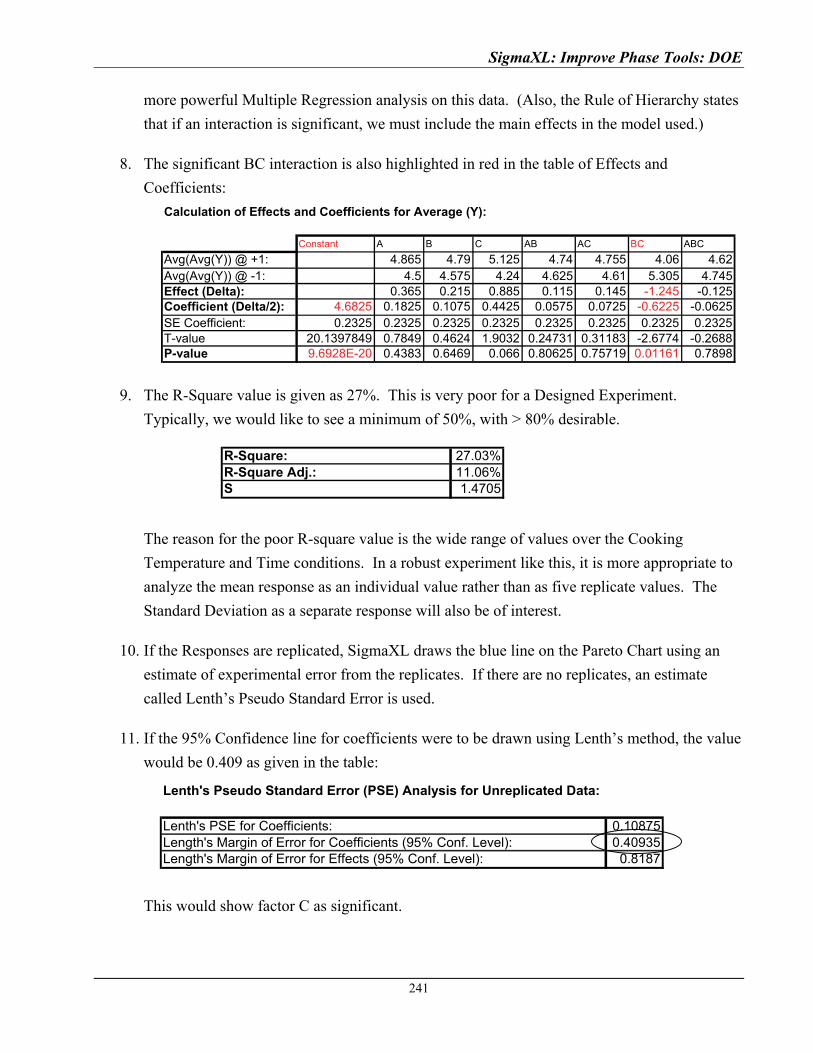
SigmaXL: Improve Phase Tools: DOE
more powerful Multiple Regression analysis on this data. (Also, the Rule of Hierarchy states
that if an interaction is significant, we must include the main effects in the model used.)
8. The significant BC interaction is also highlighted in red in the table of Effects and
Coefficients:
Calculation of Effects and Coefficients for Average (Y):
A B C AB AC ABC
Avg(Avg(Y)) @ +1: 4.865 4.79 5.125 4.74 4.755 4.06 4.62Avg(Avg(Y)) @ -1: 4.5 4.575 4.24 4.625 4.61 5.305 4.745Effect (Delta): 0.365 0.215 0.885 0.115 0.145 -0.125Coefficient (Delta/2): 0.1825 0.1075 0.4425 0.0575 0.0725 -0.0625SE Coefficient: 0.2325 0.2325 0.2325 0.2325 0.2325 0.2325 0.2325 0.2325T-value 20.1397849 0.7849 0.4624 1.9032 0.24731 0.31183 -2.6774 -0.2688P-value 0.4383 0.6469 0.066 0.80625 0.75719 0.7898
Constant BC
-1.2454.6825 -0.6225
9.6928E-20 0.01161
9. The R-Square value is given as 27%. This is very poor for a Designed Experiment.
Typically, we would like to see a minimum of 50%, with > 80% desirable.
The reason for the poor R-square value is the wide range of values over the Cooking
Temperature and Time conditions. In a robust experiment like this, it is more appropriate to
analyze the mean response as an individual value rather than as five replicate values. The
Standard Deviation as a separate response will also be of interest.
R-Square:R-Square Adj.: 11.06%S 1.4705
27.03%
10. If the Responses are replicated, SigmaXL draws the blue line on the Pareto Chart using an
estimate of experimental error from the replicates. If there are no replicates, an estimate
called Lenth’s Pseudo Standard Error is used.
11. If the 95% Confidence line for coefficients were to be drawn using Lenth’s method, the value
would be 0.409 as given in the table:
This would show factor C as significant.
Lenth's Pseudo Standard Error (PSE) Analysis for Unreplicated Data:
Lenth's PSE for Coefficients: 0.10875Length's Margin of Error for Coefficients (95% Conf. Level): 0.40935Length's Margin of Error for Effects (95% Conf. Level): 0.8187
241
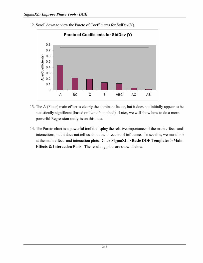
SigmaXL: Improve Phase Tools: DOE
12. Scroll down to view the Pareto of Coefficients for StdDev(Y).
Pareto of Coefficients for StdDev (Y)
0
0.1
0.2
0.3
0.4
0.5
0.6
0.7
0.8
A BC C B ABC AC AB
Ab
s(C
oef
fici
ents
)
13. The A (Flour) main effect is clearly the dominant factor, but it does not initially appear to be
statistically significant (based on Lenth’s method). Later, we will show how to do a more
powerful Regression analysis on this data.
14. The Pareto chart is a powerful tool to display the relative importance of the main effects and
interactions, but it does not tell us about the direction of influence. To see this, we must look
at the main effects and interaction plots. Click SigmaXL > Basic DOE Templates > Main
Effects & Interaction Plots. The resulting plots are shown below:
242

SigmaXL: Improve Phase Tools: DOE
15. The Butter*Egg two-factor interaction is very prominent here. Looking at only the Main
Effects plots would lead us to conclude that the optimum settings to maximize the average
taste score would be Butter = +1, and Egg = +1, but the interaction plot tells a very different
story. The correct optimum settings to maximize the taste score is Butter = -1 and Egg = +1.
16. Since Flour was the most prominent factor in the Standard Deviation Pareto, looking at the
Main Effects plots for StdDev, we would set Flour = +1 to minimize the variability in taste
scores. The significance of this result will be demonstrated using Regression analysis.
243
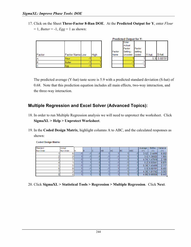
SigmaXL: Improve Phase Tools: DOE
17. Click on the Sheet Three-Factor 8-Run DOE. At the Predicted Output for Y, enter Flour
= 1, Butter = -1, Egg = 1 as shown:
The predicted average (Y-hat) taste score is 5.9 with a predicted standard deviation (S-hat) of
0.68. Note that this prediction equation includes all main effects, two-way interaction, and
the three-way interaction.
Multiple Regression and Excel Solver (Advanced Topics):
18. In order to run Multiple Regression analysis we will need to unprotect the worksheet. Click
SigmaXL > Help > Unprotect Worksheet.
19. In the Coded Design Matrix, highlight columns A to ABC, and the calculated responses as
shown:
20. Click SigmaXL > Statistical Tools > Regression > Multiple Regression. Click Next.
244
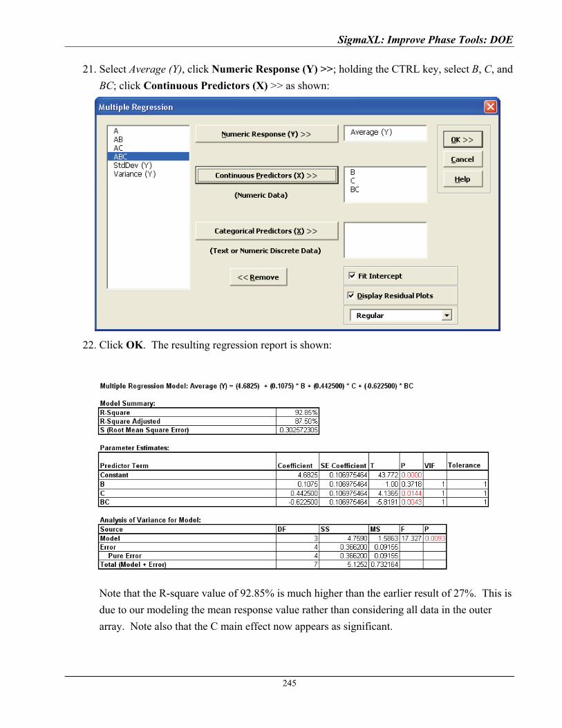
SigmaXL: Improve Phase Tools: DOE
21. Select Average (Y), click Numeric Response (Y) >>; holding the CTRL key, select B, C, and
BC; click Continuous Predictors (X) >> as shown:
22. Click OK. The resulting regression report is shown:
Note that the R-square value of 92.85% is much higher than the earlier result of 27%. This is
due to our modeling the mean response value rather than considering all data in the outer
array. Note also that the C main effect now appears as significant.
245
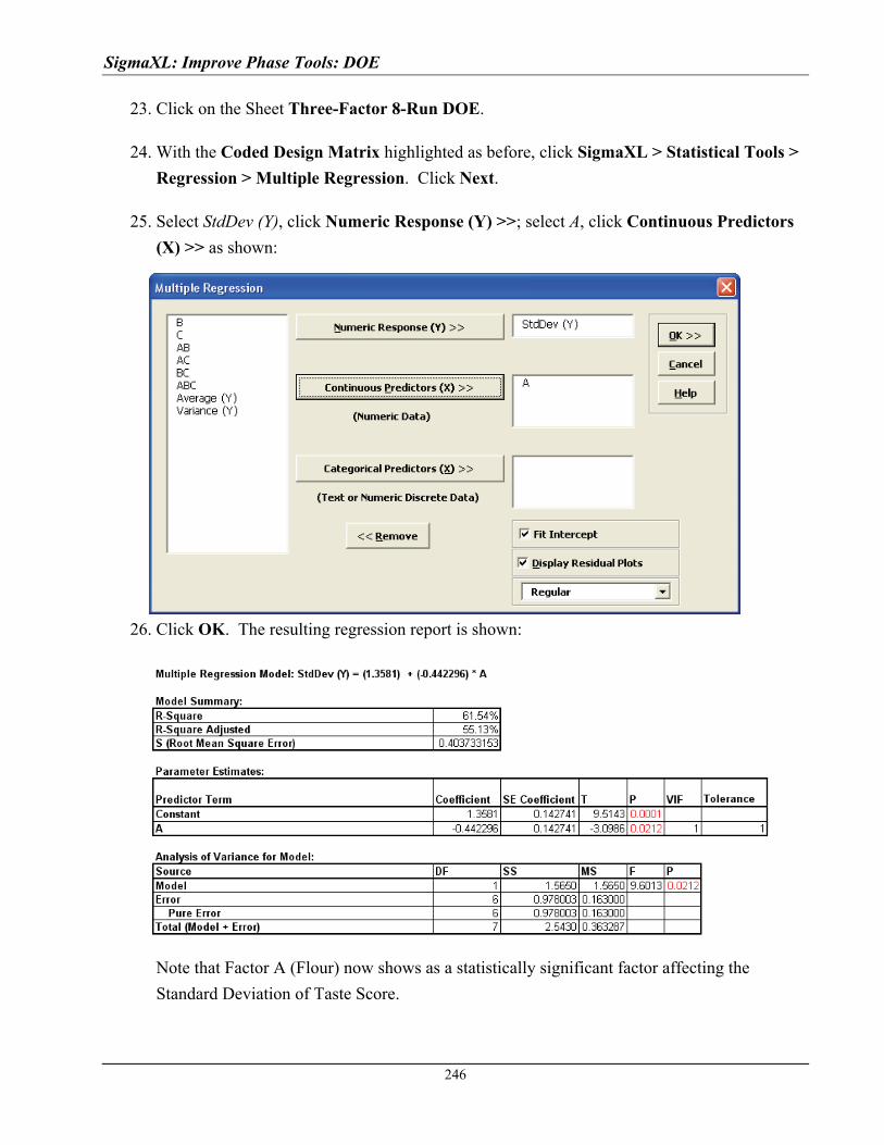
SigmaXL: Improve Phase Tools: DOE
23. Click on the Sheet Three-Factor 8-Run DOE.
24. With the Coded Design Matrix highlighted as before, click SigmaXL > Statistical Tools >
Regression > Multiple Regression. Click Next.
25. Select StdDev (Y), click Numeric Response (Y) >>; select A, click Continuous Predictors
(X) >> as shown:
26. Click OK. The resulting regression report is shown:
Note that Factor A (Flour) now shows as a statistically significant factor affecting the
Standard Deviation of Taste Score.
246
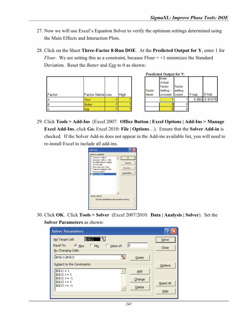
SigmaXL: Improve Phase Tools: DOE
27. Now we will use Excel’s Equation Solver to verify the optimum settings determined using
the Main Effects and Interaction Plots.
28. Click on the Sheet Three-Factor 8-Run DOE. At the Predicted Output for Y, enter 1 for
Flour. We are setting this as a constraint, because Flour = +1 minimizes the Standard
Deviation. Reset the Butter and Egg to 0 as shown:
29. Click Tools > Add-Ins (Excel 2007: Office Button | Excel Options | Add-Ins > Manage
Excel Add-Ins, click Go; Excel 2010: File | Options…). Ensure that the Solver Add-in is
checked. If the Solver Add-in does not appear in the Add-ins available list, you will need to
re-install Excel to include all add-ins.
30. Click OK. Click Tools > Solver (Excel 2007/2010: Data | Analysis | Solver). Set the
Solver Parameters as shown:
247
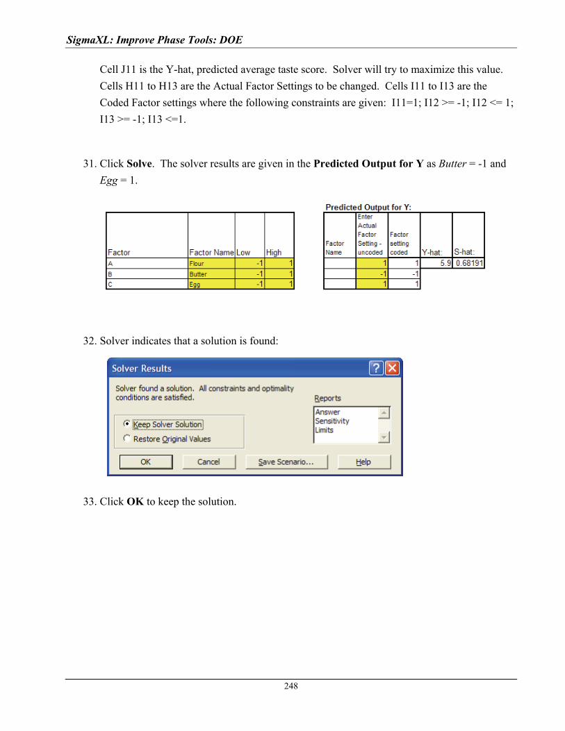
SigmaXL: Improve Phase Tools: DOE
Cell J11 is the Y-hat, predicted average taste score. Solver will try to maximize this value.
Cells H11 to H13 are the Actual Factor Settings to be changed. Cells I11 to I13 are the
Coded Factor settings where the following constraints are given: I11=1; I12 >= -1; I12 <= 1;
I13 >= -1; I13 <=1.
31. Click Solve. The solver results are given in the Predicted Output for Y as Butter = -1 and
Egg = 1.
32. Solver indicates that a solution is found:
33. Click OK to keep the solution.
248

SigmaXL: Improve Phase Tools: DOE
Part C – Design and Analysis of Catapult Full Factorial Experiment
Catapults are frequently used in Six-Sigma or Design of
Experiments training. They are a powerful teaching tool and make
the learning fun. If you have access to a catapult, we recommend
that you perform the actual experiment and use your own data. Of
course, you can also follow along using the data provided. The
response variable (Y) is distance, with the goal being to
consistently hit a target of 100 inches.
1. Click SigmaXL > Design of Experiments > 2-Level
Factorial/Screening > 2-Level Factorial/Screening Designs.
2. The Number of X Factors can be 2 to 19. Using process knowledge, we will limit ourselves
to 3 factors: Pull Back Angle, Stop Pin and Pin Height. Pull Back will be varied from 160 to
180 degrees, Stop Pin will be positions 2 and 3 (count from the back), and Pin Height will be
positions 2 and 3 (count from the bottom).
3. Select Number of Factors = 3.
4. The available designs are then given as: 4-Run, 2**(3-1), 1/2 Fraction, Res III and 8-Run,
2**3, Full-Factorial. If we had more than 5 factors, a Resolution III or Plackett-Burman
Screening design would typically be used. Here we will choose the 8-Run, 2**3, Full-
Factorial design.
249

SigmaXL: Improve Phase Tools: DOE
5. Next we will review the Power Information to help us determine the number of replicates.
This design currently shows the following:
These power calculations assume 3 center points:
Very Low Power to detect Effect = 1*StDev (1-Beta < 0.5);
Very Low Power to detect Effect = 2*StDev (1-Beta < 0.5);
Medium Power to detect Effect = 3*StDev (0.8 <= 1-Beta < 0.95).
Note: the power calculations require an estimate of experimental error, hence an assumption
of 3 center points is used.
We would like to have a reasonable chance (medium power) to detect an Effect = 2*StDev.
Change the Number of Replicates to 2. The Power Information is now:
Very Low Power to detect Effect = 1*StDev (1-Beta < 0.5);
Medium Power to detect Effect = 2*StDev (0.8 <= 1-Beta < 0.95);
Very High Power to detect Effect = 3*StDev (1-Beta >= 0.99).
We will therefore choose two replicates. The number of replicates will always be a tradeoff
between the desired power and the cost of the experimental runs.
Specify 2 or more blocks if there are constraints such as the number of runs per day or some
other known external “nuisance” variable (like 2 different catapults or 2 operators). Here we
will keep Blocks = 1 (i.e. no Blocking).
250
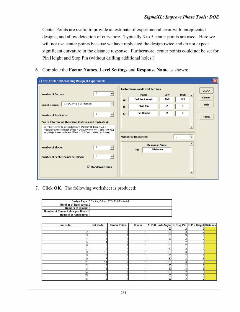
SigmaXL: Improve Phase Tools: DOE
Center Points are useful to provide an estimate of experimental error with unreplicated
designs, and allow detection of curvature. Typically 3 to 5 center points are used. Here we
will not use center points because we have replicated the design twice and do not expect
significant curvature in the distance response. Furthermore, center points could not be set for
Pin Height and Stop Pin (without drilling additional holes!).
6. Complete the Factor Names, Level Settings and Response Name as shown:
7. Click OK. The following worksheet is produced:
251
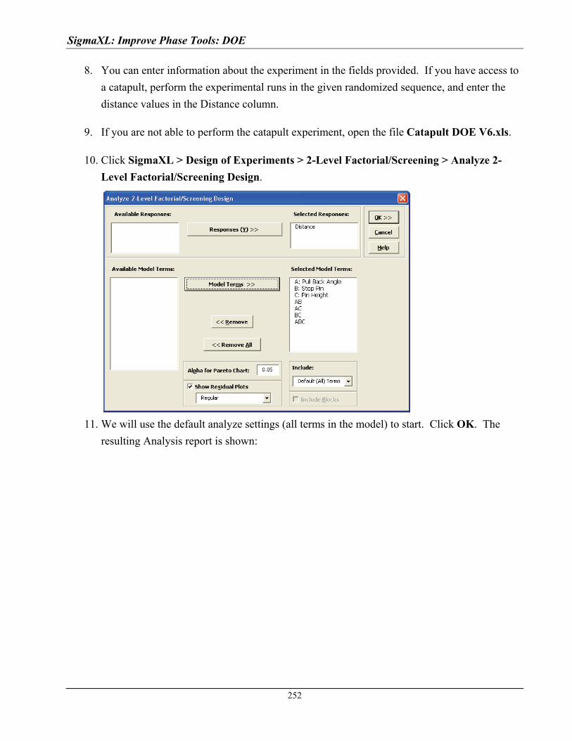
SigmaXL: Improve Phase Tools: DOE
8. You can enter information about the experiment in the fields provided. If you have access to
a catapult, perform the experimental runs in the given randomized sequence, and enter the
distance values in the Distance column.
9. If you are not able to perform the catapult experiment, open the file Catapult DOE V6.xls.
10. Click SigmaXL > Design of Experiments > 2-Level Factorial/Screening > Analyze 2-
Level Factorial/Screening Design.
11. We will use the default analyze settings (all terms in the model) to start. Click OK. The
resulting Analysis report is shown:
252
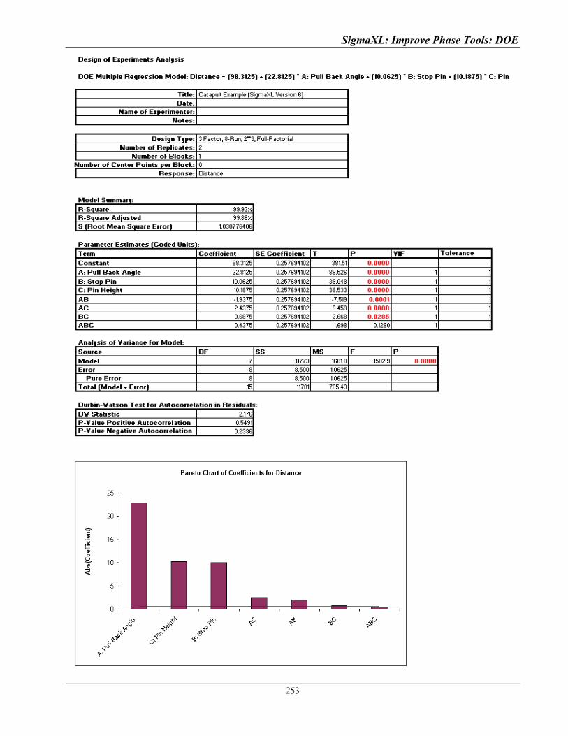
SigmaXL: Improve Phase Tools: DOE
253

SigmaXL: Improve Phase Tools: DOE
12. The model looks very good with an R-Square value of 99.9%! The standard deviation
(experimental error) is only 1.03 inches. Clearly Pull Back Angle is the most important
predictor (X factor), but all the main effects and two way interaction are significant.
However, the three-way interaction is not significant, so it should be removed from the
model.
13. Click Recall Last Dialog (or press F3).
14. Remove the ABC interaction term as shown:
15. Click OK. The revised report is shown below:
254
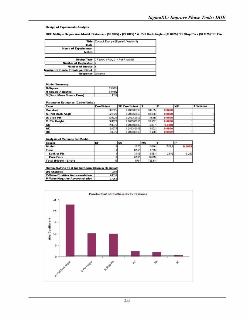
SigmaXL: Improve Phase Tools: DOE
255
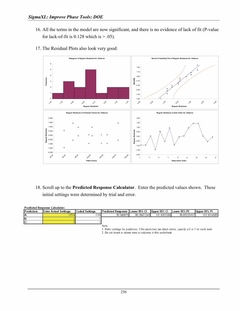
SigmaXL: Improve Phase Tools: DOE
16. All the terms in the model are now significant, and there is no evidence of lack of fit (P-value
for lack-of-fit is 0.128 which is > .05).
17. The Residual Plots also look very good:
Histogram of Regular Residuals for: Distance
0
1
2
3
4
5
6
-1.44
-1.03
-0.62
-0.20 0.
210.
621.
031.
44
Regular Residuals
Fre
qu
ency
Normal Probability Plot of Regular Residuals for: Distance
-1.90
-1.40
-0.90
-0.40
0.10
0.60
1.10
1.60
-3.00
-2.00
-1.00 0.
001.
002.
003.
00
Regular Residuals
NS
CO
RE
Regular Residuals vs Predicted Values for: Distance
-2.000
-1.500
-1.000
-0.500
0.000
0.500
1.000
1.500
2.000
40.00
60.00
80.00
100.0
0
120.0
0
140.0
0
160.0
0
Fitted Values
Reg
ula
r R
esid
ual
s
Regular Residuals vs Data Order for: Distance
-2.00
-1.50
-1.00
-0.50
0.00
0.50
1.00
1.50
2.00
1 3 5 7 9 11 13 15 17
Observation Order
Reg
ula
r R
esid
ual
s
18. Scroll up to the Predicted Response Calculator. Enter the predicted values shown. These
initial settings were determined by trial and error.
256
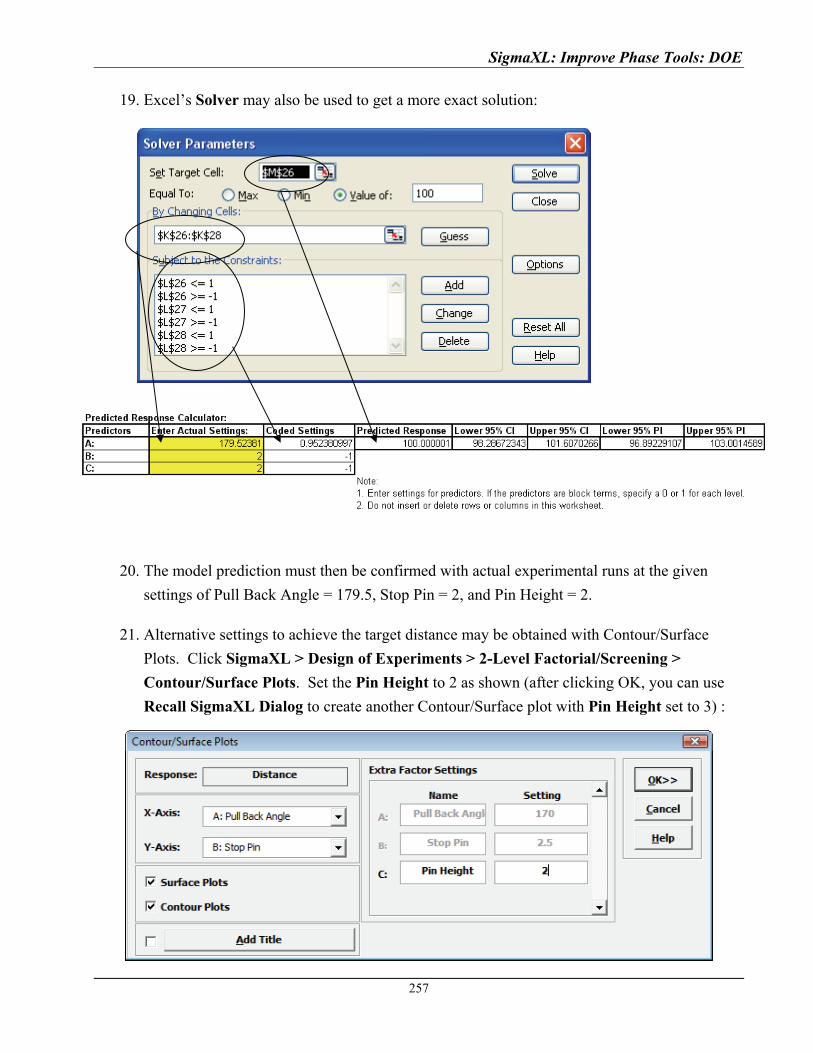
SigmaXL: Improve Phase Tools: DOE
19. Excel’s Solver may also be used to get a more exact solution:
20. The model prediction must then be confirmed with actual experimental runs at the given
settings of Pull Back Angle = 179.5, Stop Pin = 2, and Pin Height = 2.
21. Alternative settings to achieve the target distance may be obtained with Contour/Surface
Plots. Click SigmaXL > Design of Experiments > 2-Level Factorial/Screening >
Contour/Surface Plots. Set the Pin Height to 2 as shown (after clicking OK, you can use
Recall SigmaXL Dialog to create another Contour/Surface plot with Pin Height set to 3) :
257
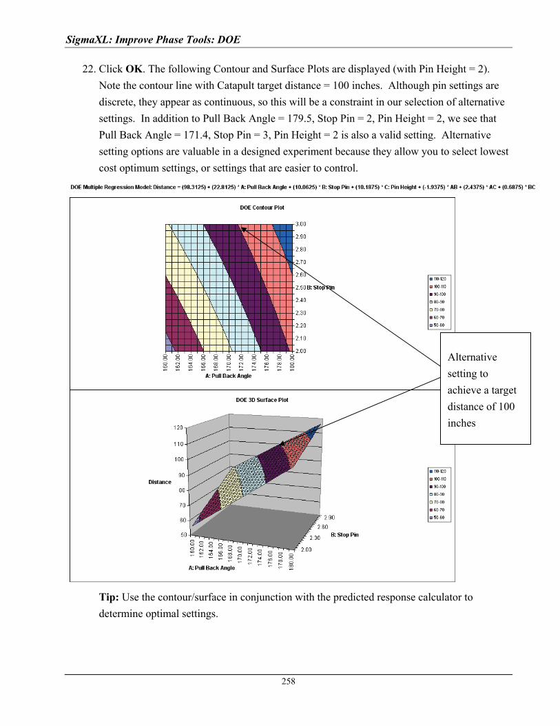
SigmaXL: Improve Phase Tools: DOE
22. Click OK. The following Contour and Surface Plots are displayed (with Pin Height = 2).
Note the contour line with Catapult target distance = 100 inches. Although pin settings are
discrete, they appear as continuous, so this will be a constraint in our selection of alternative
settings. In addition to Pull Back Angle = 179.5, Stop Pin = 2, Pin Height = 2, we see that
Pull Back Angle = 171.4, Stop Pin = 3, Pin Height = 2 is also a valid setting. Alternative
setting options are valuable in a designed experiment because they allow you to select lowest
cost optimum settings, or settings that are easier to control.
Tip: Use the contour/surface in conjunction with the predicted response calculator to
determine optimal settings.
Alternative
setting to
achieve a target
distance of 100
inches
258
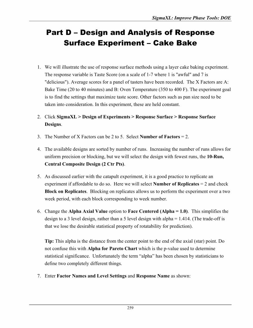
SigmaXL: Improve Phase Tools: DOE
259
Part D – Design and Analysis of Response Surface Experiment – Cake Bake
1. We will illustrate the use of response surface methods using a layer cake baking experiment.
The response variable is Taste Score (on a scale of 1-7 where 1 is "awful" and 7 is
"delicious"). Average scores for a panel of tasters have been recorded. The X Factors are A:
Bake Time (20 to 40 minutes) and B: Oven Temperature (350 to 400 F). The experiment goal
is to find the settings that maximize taste score. Other factors such as pan size need to be
taken into consideration. In this experiment, these are held constant.
2. Click SigmaXL > Design of Experiments > Response Surface > Response Surface
Designs.
3. The Number of X Factors can be 2 to 5. Select Number of Factors = 2.
4. The available designs are sorted by number of runs. Increasing the number of runs allows for
uniform precision or blocking, but we will select the design with fewest runs, the 10-Run,
Central Composite Design (2 Ctr Pts).
5. As discussed earlier with the catapult experiment, it is a good practice to replicate an
experiment if affordable to do so. Here we will select Number of Replicates = 2 and check
Block on Replicates. Blocking on replicates allows us to perform the experiment over a two
week period, with each block corresponding to week number.
6. Change the Alpha Axial Value option to Face Centered (Alpha = 1.0). This simplifies the
design to a 3 level design, rather than a 5 level design with alpha = 1.414. (The trade-off is
that we lose the desirable statistical property of rotatability for prediction).
Tip: This alpha is the distance from the center point to the end of the axial (star) point. Do
not confuse this with Alpha for Pareto Chart which is the p-value used to determine
statistical significance. Unfortunately the term “alpha” has been chosen by statisticians to
define two completely different things.
7. Enter Factor Names and Level Settings and Response Name as shown:
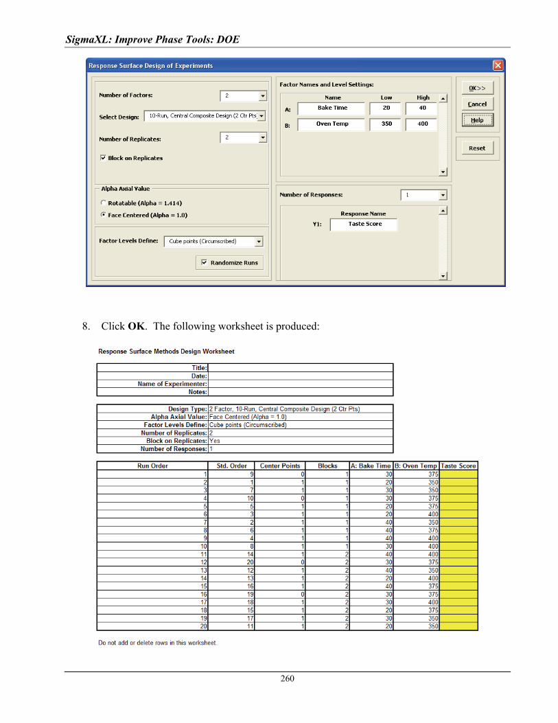
SigmaXL: Improve Phase Tools: DOE
8. Click OK. The following worksheet is produced:
260
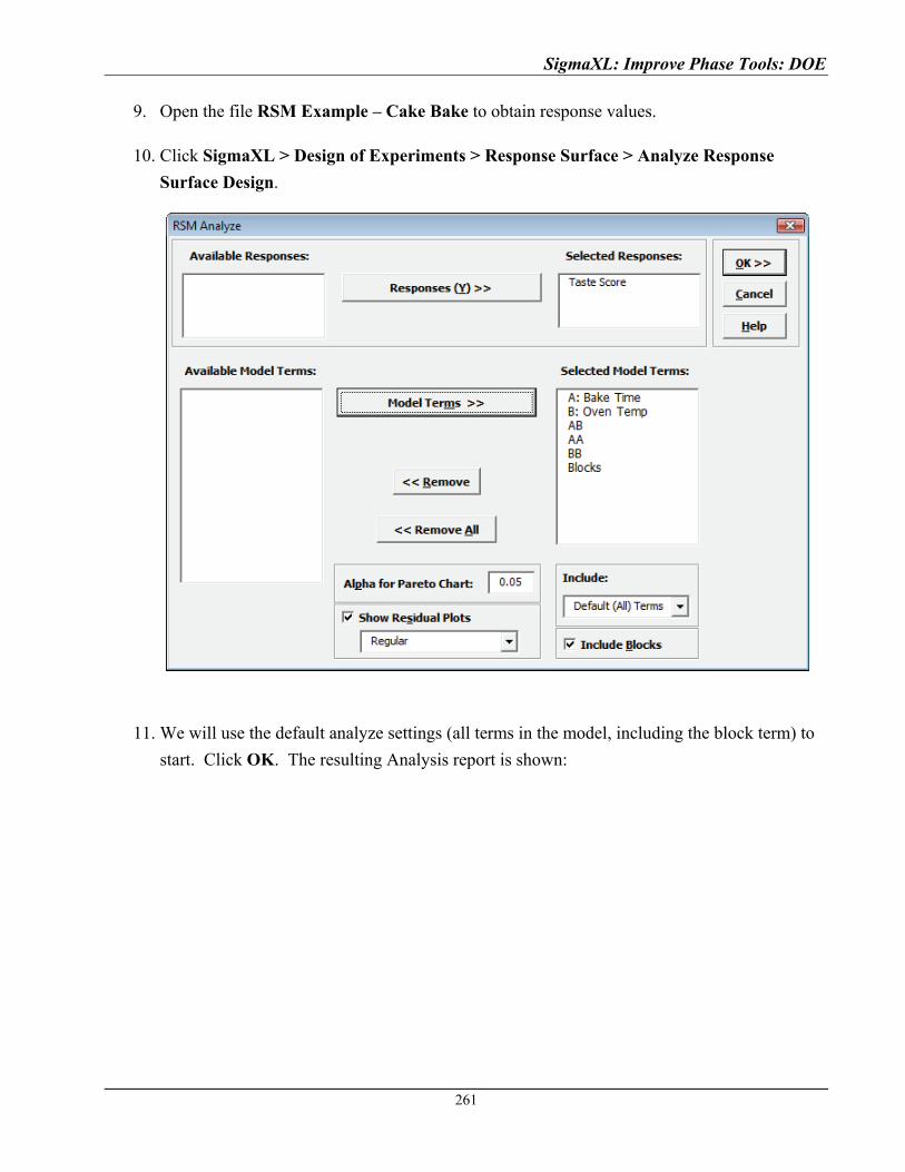
SigmaXL: Improve Phase Tools: DOE
9. Open the file RSM Example – Cake Bake to obtain response values.
10. Click SigmaXL > Design of Experiments > Response Surface > Analyze Response
Surface Design.
11. We will use the default analyze settings (all terms in the model, including the block term) to
start. Click OK. The resulting Analysis report is shown:
261
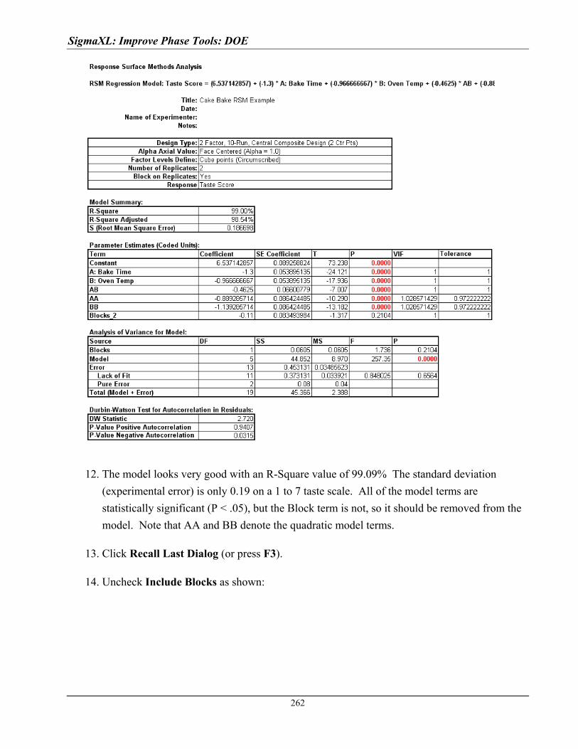
SigmaXL: Improve Phase Tools: DOE
12. The model looks very good with an R-Square value of 99.09% The standard deviation
(experimental error) is only 0.19 on a 1 to 7 taste scale. All of the model terms are
statistically significant (P < .05), but the Block term is not, so it should be removed from the
model. Note that AA and BB denote the quadratic model terms.
13. Click Recall Last Dialog (or press F3).
14. Uncheck Include Blocks as shown:
262

SigmaXL: Improve Phase Tools: DOE
15. Click OK. The revised report is shown below:
263
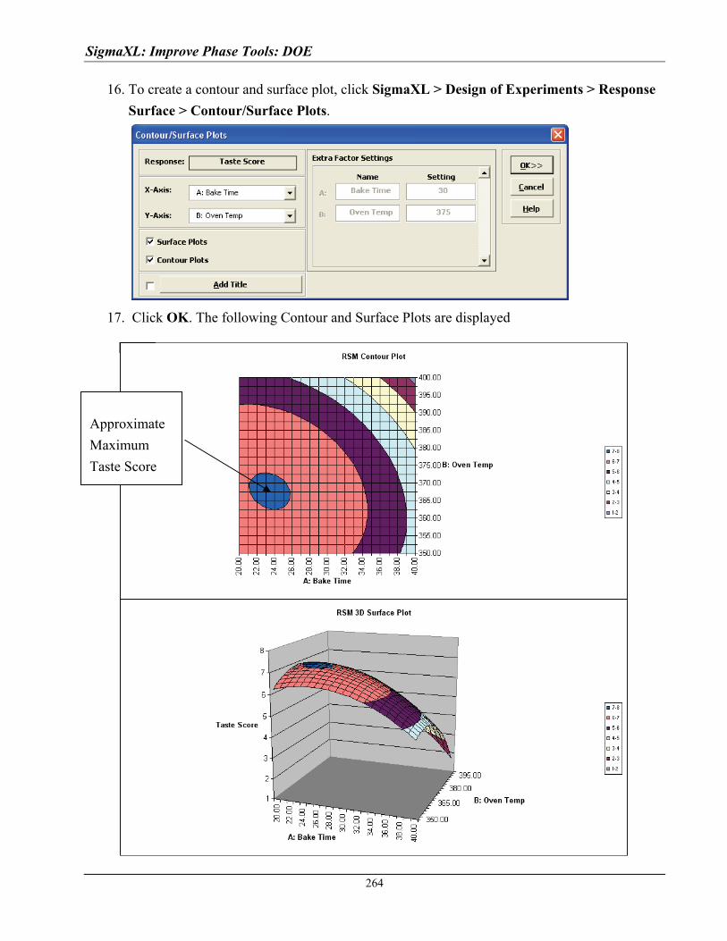
SigmaXL: Improve Phase Tools: DOE
16. To create a contour and surface plot, click SigmaXL > Design of Experiments > Response
Surface > Contour/Surface Plots.
17. Click OK. The following Contour and Surface Plots are displayed
Approximate
Maximum
Taste Score
264
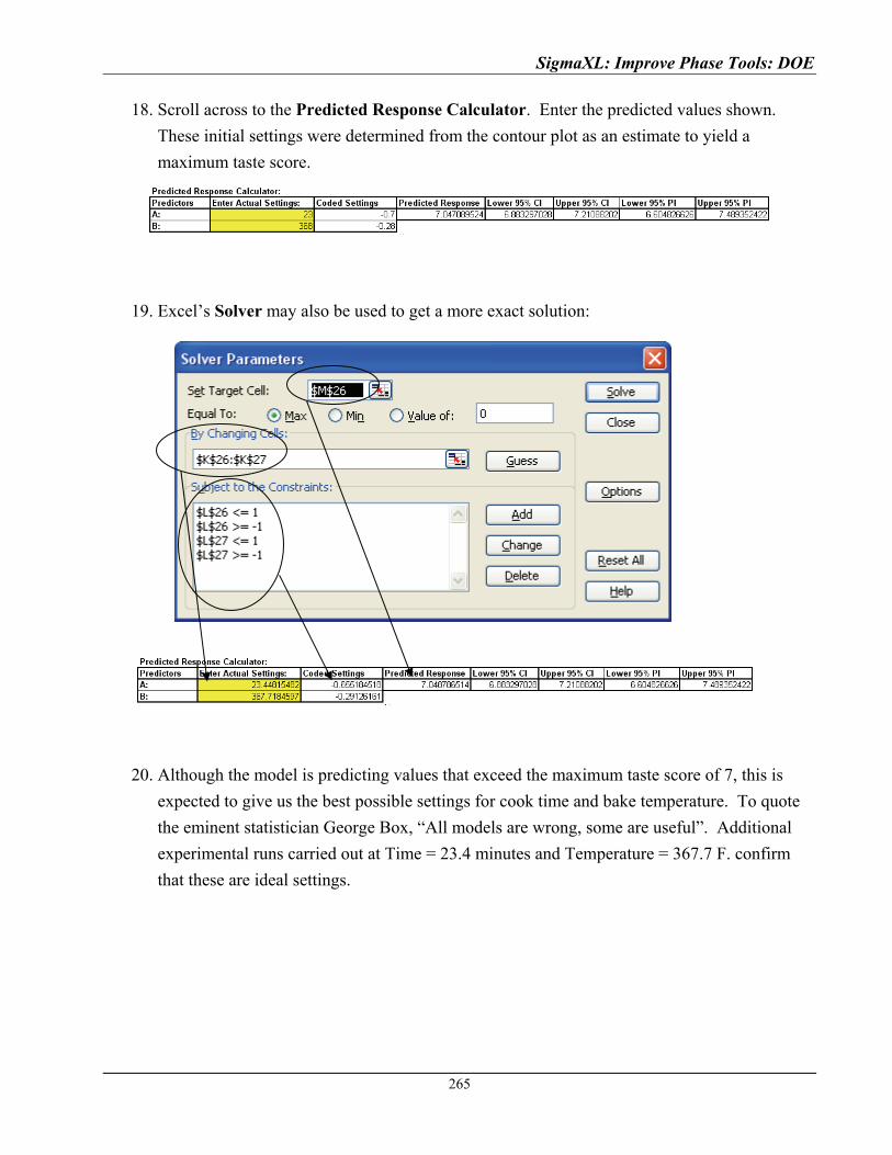
SigmaXL: Improve Phase Tools: DOE
18. Scroll across to the Predicted Response Calculator. Enter the predicted values shown.
These initial settings were determined from the contour plot as an estimate to yield a
maximum taste score.
19. Excel’s Solver may also be used to get a more exact solution:
20. Although the model is predicting values that exceed the maximum taste score of 7, this is
expected to give us the best possible settings for cook time and bake temperature. To quote
the eminent statistician George Box, “All models are wrong, some are useful”. Additional
experimental runs carried out at Time = 23.4 minutes and Temperature = 367.7 F. confirm
that these are ideal settings.
265

Copyright © 2004-2011, SigmaXL Inc.
SigmaXL: Control Phase Tools: Statistical Process Control (SPC)
Charts


SigmaXL: Control Phase Tools: SPC
269
Part A - Individuals Charts
Individuals Charts
1. Open Customer Data.xls, click on Sheet 1. Click SigmaXL>Control Charts>Individuals.
Ensure that entire data table is selected. If not, check Use Entire Data Table. Click Next.
2. Select Overall Satisfaction, click Numeric Data Variable (Y) >>. Ensure that Calculate
Limits is selected.
3. Click OK. Resulting Individuals control chart:
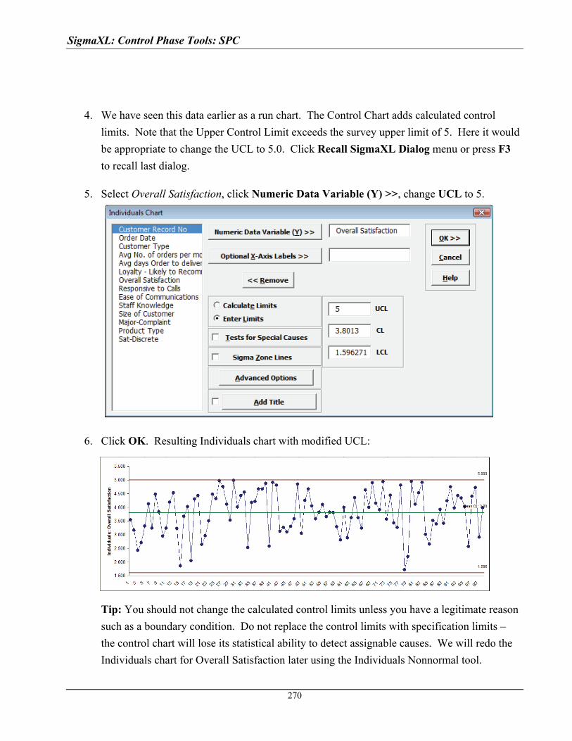
SigmaXL: Control Phase Tools: SPC
4. We have seen this data earlier as a run chart. The Control Chart adds calculated control
limits. Note that the Upper Control Limit exceeds the survey upper limit of 5. Here it would
be appropriate to change the UCL to 5.0. Click Recall SigmaXL Dialog menu or press F3
to recall last dialog.
5. Select Overall Satisfaction, click Numeric Data Variable (Y) >>, change UCL to 5.
6. Click OK. Resulting Individuals chart with modified UCL:
Tip: You should not change the calculated control limits unless you have a legitimate reason
such as a boundary condition. Do not replace the control limits with specification limits –
the control chart will lose its statistical ability to detect assignable causes. We will redo the
Individuals chart for Overall Satisfaction later using the Individuals Nonnormal tool.
270

SigmaXL: Control Phase Tools: SPC
271
7. Open Delivery Times.xls. Click Sheet 1 Tab. This data set contains room service delivery
time deviations in minutes. The Critical Customer Requirement is target time +/- 10
minutes.
8. Click SigmaXL > Control Charts > Individuals. Ensure that entire data table is selected.
If not, check Use Entire Data Table. Click Next.
9. Select Delivery Time Deviation, click Numeric Data Variable (Y) >>, check Tests for
Special Causes, check Sigma Zone Lines. Ensure that Calculate Limits is selected.
10. Select Advanced Options, specify LSL = -10, Target = 0, USL = 10 as shown:
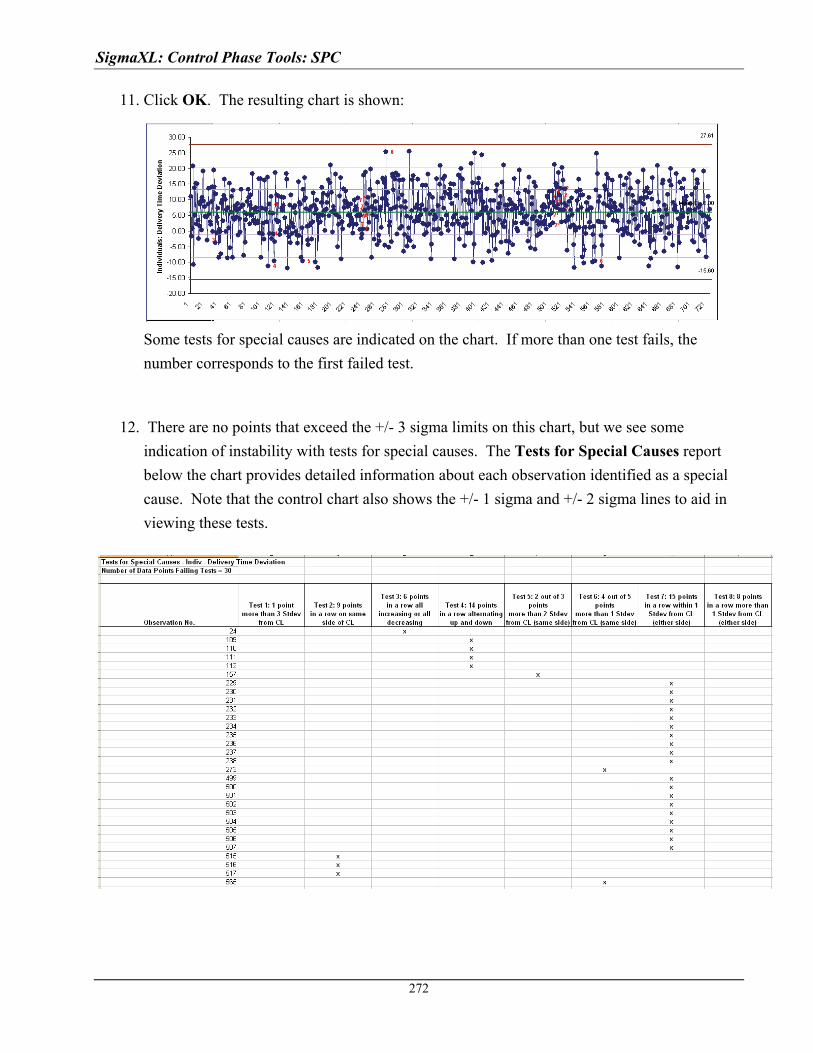
SigmaXL: Control Phase Tools: SPC
11. Click OK. The resulting chart is shown:
Some tests for special causes are indicated on the chart. If more than one test fails, the
number corresponds to the first failed test.
12. There are no points that exceed the +/- 3 sigma limits on this chart, but we see some
indication of instability with tests for special causes. The Tests for Special Causes report
below the chart provides detailed information about each observation identified as a special
cause. Note that the control chart also shows the +/- 1 sigma and +/- 2 sigma lines to aid in
viewing these tests.
272
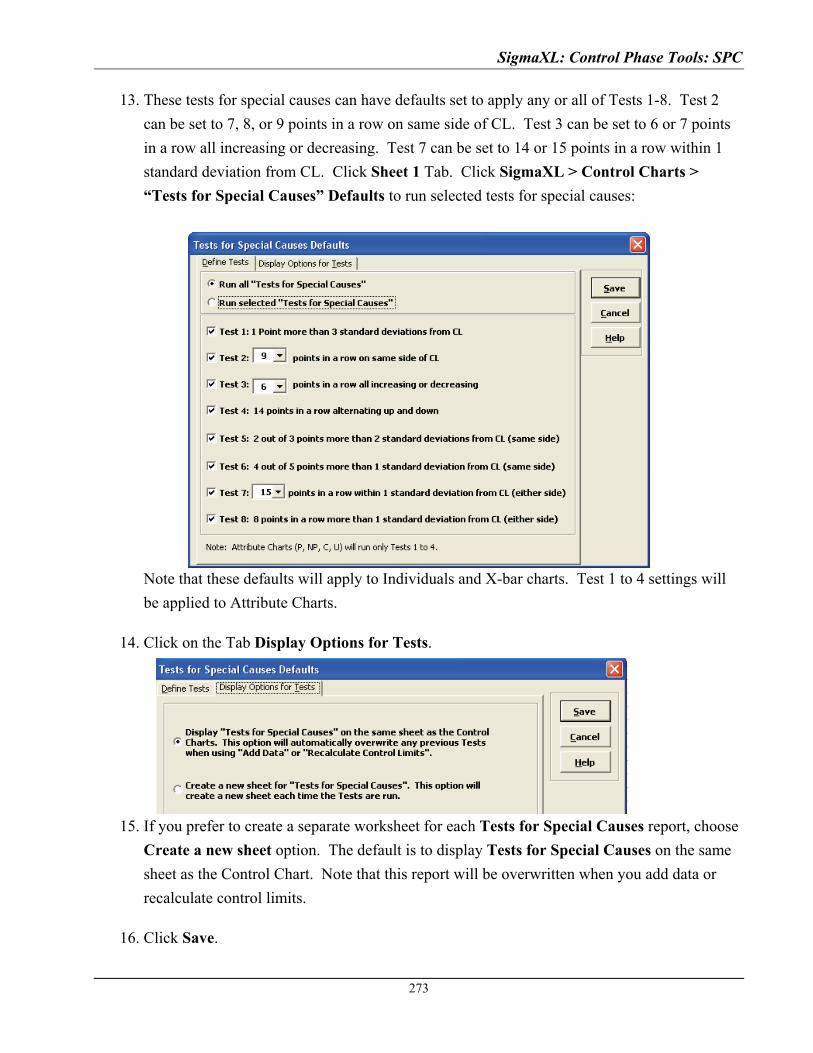
SigmaXL: Control Phase Tools: SPC
273
13. These tests for special causes can have defaults set to apply any or all of Tests 1-8. Test 2
can be set to 7, 8, or 9 points in a row on same side of CL. Test 3 can be set to 6 or 7 points
in a row all increasing or decreasing. Test 7 can be set to 14 or 15 points in a row within 1
standard deviation from CL. Click Sheet 1 Tab. Click SigmaXL > Control Charts >
“Tests for Special Causes” Defaults to run selected tests for special causes:
Note that these defaults will apply to Individuals and X-bar charts. Test 1 to 4 settings will
be applied to Attribute Charts.
14. Click on the Tab Display Options for Tests.
15. If you prefer to create a separate worksheet for each Tests for Special Causes report, choose
Create a new sheet option. The default is to display Tests for Special Causes on the same
sheet as the Control Chart. Note that this report will be overwritten when you add data or
recalculate control limits.
16. Click Save.

SigmaXL: Control Phase Tools: SPC
17. Click on Indiv Proc Cap Tab to view the Process Capability Report, which includes
potential (short term) capability indices Cp and Cpk:
18. While this process demonstrated some slight instability on the control charts, the bigger issue
was being late 6 minutes on average and having a Standard Deviation of 7.2 minutes! One
improvement implemented was rescheduling the service elevators so that Room Service and
Maintenance were not both trying to use them during peak times.
274

SigmaXL: Control Phase Tools: SPC
275
19. Click on the Indiv sheet. With 725 data points, you may want to have a closer look at the
most recent data. To do this, click SigmaXL Chart Tools > Show Last 30 Points. (If this
menu item does not appear, click on any cell adjacent to the chart.) The resulting chart is
shown:
20. To reset the chart, click SigmaXL Chart Tools > Show All Data Points.
21. To enable scrolling, click SigmaXL Chart Tools > Enable Scrolling. A warning message
is given:
Scrolling will clear user custom formats, but does not affect Tests for Special Causes.
22. Click OK. A scroll dialog appears allowing you to specify the Start Subgroup and
Window Width:
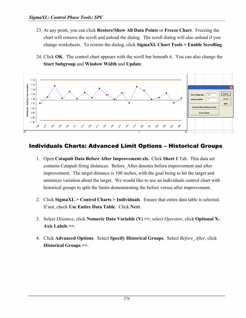
SigmaXL: Control Phase Tools: SPC
23. At any point, you can click Restore/Show All Data Points or Freeze Chart. Freezing the
chart will remove the scroll and unload the dialog. The scroll dialog will also unload if you
change worksheets. To restore the dialog, click SigmaXL Chart Tools > Enable Scrolling.
24. Click OK. The control chart appears with the scroll bar beneath it. You can also change the
Start Subgroup and Window Width and Update.
Individuals Charts: Advanced Limit Options – Historical Groups
1. Open Catapult Data Before After Improvement.xls. Click Sheet 1 Tab. This data set
contains Catapult firing distances. Before_After denotes before improvement and after
improvement. The target distance is 100 inches, with the goal being to hit the target and
minimize variation about the target. We would like to use an individuals control chart with
historical groups to split the limits demonstrating the before versus after improvement.
2. Click SigmaXL > Control Charts > Individuals. Ensure that entire data table is selected.
If not, check Use Entire Data Table. Click Next.
3. Select Distance, click Numeric Data Variable (Y) >>; select Operator, click Optional X-
Axis Labels >>.
4. Click Advanced Options. Select Specify Historical Groups. Select Before_After, click
Historical Groups >>.
276
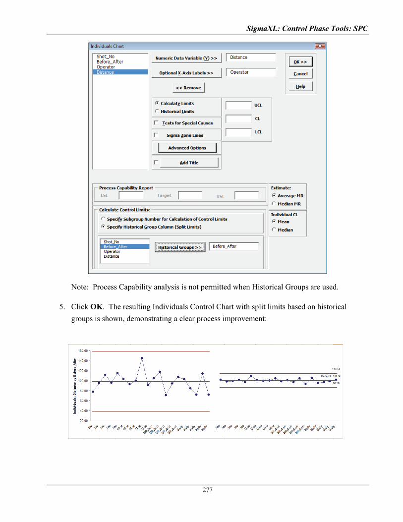
SigmaXL: Control Phase Tools: SPC
277
Note: Process Capability analysis is not permitted when Historical Groups are used.
5. Click OK. The resulting Individuals Control Chart with split limits based on historical
groups is shown, demonstrating a clear process improvement:
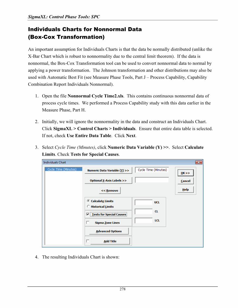
SigmaXL: Control Phase Tools: SPC
Individuals Charts for Nonnormal Data (Box-Cox Transformation)
An important assumption for Individuals Charts is that the data be normally distributed (unlike the
X-Bar Chart which is robust to nonnormality due to the central limit theorem). If the data is
nonnormal, the Box-Cox Transformation tool can be used to convert nonnormal data to normal by
applying a power transformation. The Johnson transformation and other distributions may also be
used with Automatic Best Fit (see Measure Phase Tools, Part J – Process Capability, Capability
Combination Report Individuals Nonnormal).
1. Open the file Nonnormal Cycle Time2.xls. This contains continuous nonnormal data of
process cycle times. We performed a Process Capability study with this data earlier in the
Measure Phase, Part H.
2. Initially, we will ignore the nonnormality in the data and construct an Individuals Chart.
Click SigmaXL > Control Charts > Individuals. Ensure that entire data table is selected.
If not, check Use Entire Data Table. Click Next.
3. Select Cycle Time (Minutes), click Numeric Data Variable (Y) >>. Select Calculate
Limits. Check Tests for Special Causes.
4. The resulting Individuals Chart is shown:
278
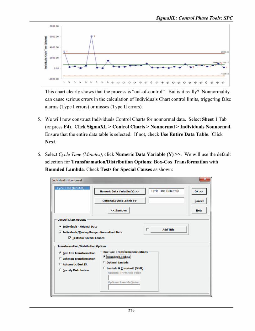
SigmaXL: Control Phase Tools: SPC
279
This chart clearly shows that the process is “out-of-control”. But is it really? Nonnormality
can cause serious errors in the calculation of Individuals Chart control limits, triggering false
alarms (Type I errors) or misses (Type II errors).
5. We will now construct Individuals Control Charts for nonnormal data. Select Sheet 1 Tab
(or press F4). Click SigmaXL > Control Charts > Nonnormal > Individuals Nonnormal.
Ensure that the entire data table is selected. If not, check Use Entire Data Table. Click
Next.
6. Select Cycle Time (Minutes), click Numeric Data Variable (Y) >>. We will use the default
selection for Transformation/Distribution Options: Box-Cox Transformation with
Rounded Lambda. Check Tests for Special Causes as shown:
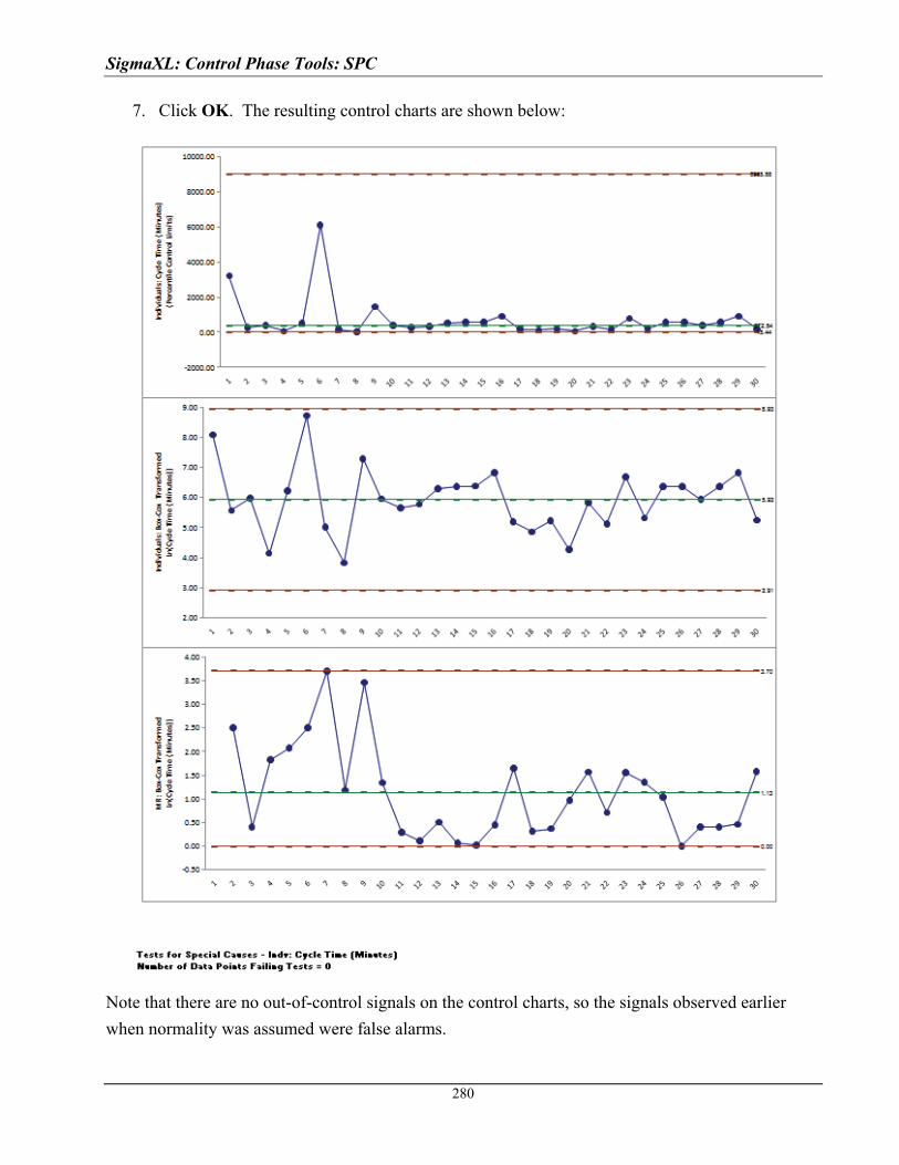
SigmaXL: Control Phase Tools: SPC
7. Click OK. The resulting control charts are shown below:
Note that there are no out-of-control signals on the control charts, so the signals observed earlier
when normality was assumed were false alarms.
280
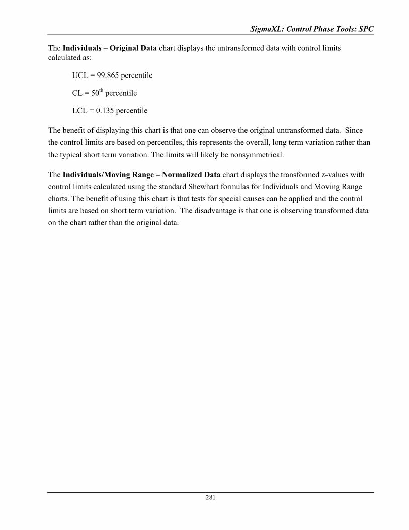
SigmaXL: Control Phase Tools: SPC
281
The Individuals – Original Data chart displays the untransformed data with control limits calculated as:
UCL = 99.865 percentile
CL = 50th percentile
LCL = 0.135 percentile
The benefit of displaying this chart is that one can observe the original untransformed data. Since
the control limits are based on percentiles, this represents the overall, long term variation rather than
the typical short term variation. The limits will likely be nonsymmetrical.
The Individuals/Moving Range – Normalized Data chart displays the transformed z-values with
control limits calculated using the standard Shewhart formulas for Individuals and Moving Range
charts. The benefit of using this chart is that tests for special causes can be applied and the control
limits are based on short term variation. The disadvantage is that one is observing transformed data
on the chart rather than the original data.
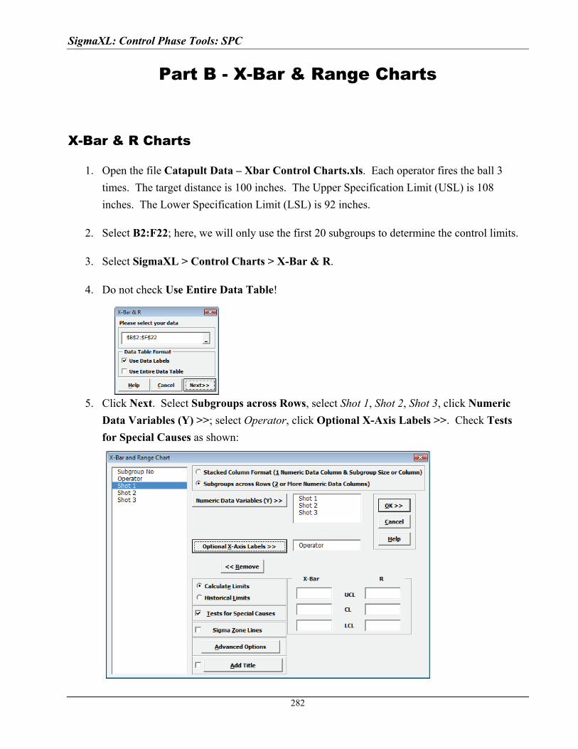
SigmaXL: Control Phase Tools: SPC
Part B - X-Bar & Range Charts
X-Bar & R Charts
1. Open the file Catapult Data – Xbar Control Charts.xls. Each operator fires the ball 3
times. The target distance is 100 inches. The Upper Specification Limit (USL) is 108
inches. The Lower Specification Limit (LSL) is 92 inches.
2. Select B2:F22; here, we will only use the first 20 subgroups to determine the control limits.
3. Select SigmaXL > Control Charts > X-Bar & R.
4. Do not check Use Entire Data Table!
5. Click Next. Select Subgroups across Rows, select Shot 1, Shot 2, Shot 3, click Numeric
Data Variables (Y) >>; select Operator, click Optional X-Axis Labels >>. Check Tests
for Special Causes as shown:
282
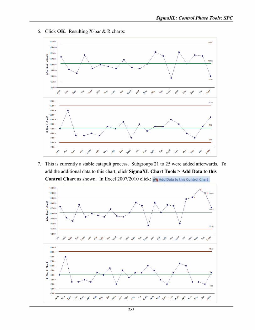
SigmaXL: Control Phase Tools: SPC
283
6. Click OK. Resulting X-bar & R charts:
7. This is currently a stable catapult process. Subgroups 21 to 25 were added afterwards. To
add the additional data to this chart, click SigmaXL Chart Tools > Add Data to this
Control Chart as shown. In Excel 2007/2010 click:

SigmaXL: Control Phase Tools: SPC
8. Note that the Add Data button does NOT recalculate the control limits. Once control limits
are established, they should only be recalculated when a deliberate process change or
improvement is introduced. (Control Limits can be recalculated using SigmaXL Chart
Tools > Recalculate Control Limits, but a warning message Are you sure that you want
to recalculate control limits? is given.)
9. The Tests for Special Causes report gives us more detail on the recent instability:
The X-bar chart and Tests for Special Causes report clearly shows that this process is now
out of control with an unstable mean. The process must be stopped, and the Out-of-Control
Action Plan must be followed to determine and fix the root cause. In this case, the assignable
cause was a change of rubber band requiring a reset of the pull back angle. The use of tests
for special causes gave us an early warning of this at observation number 22.
Note that the Range chart is in-control even though the X-Bar chart is out-of-control.
10. The tests for special causes can have defaults set to apply any or all of Tests 1-8. Test 2 can
be set to 7, 8, or 9 points in a row on same side of CL. Click SigmaXL > Control Charts >
“Tests for Special Causes” Defaults to run selected tests for special causes. (Note that
these defaults will apply to Individuals and X-bar charts. Test 1 to 4 settings will be applied
to Attribute Charts.)
11. To add a comment to a data point, select SigmaXL Chart Tools > Add Data Label. Select
Text Label. Enter a comment as shown. Click on the data point to add the comment. Click
Done.
284

SigmaXL: Control Phase Tools: SPC
285
12. Now we will look at Process Capability Indices for this process. Click on Sheet 1 (or press
F4 to activate last worksheet). Click SigmaXL > Control Charts > X-Bar & R. Check
Use Entire Data Table. Click Next. (Alternatively select B2:F27, press F3.)
13. Select Shots 1-3, click Numeric Data Variables (Y) >>. Select Historical Limits. These
are the limits calculated with the original 20 subgroups.
14. Click Advanced Options. Enter LSL = 92, Target = 100, USL = 108.
15. The resulting dialog box settings are shown:
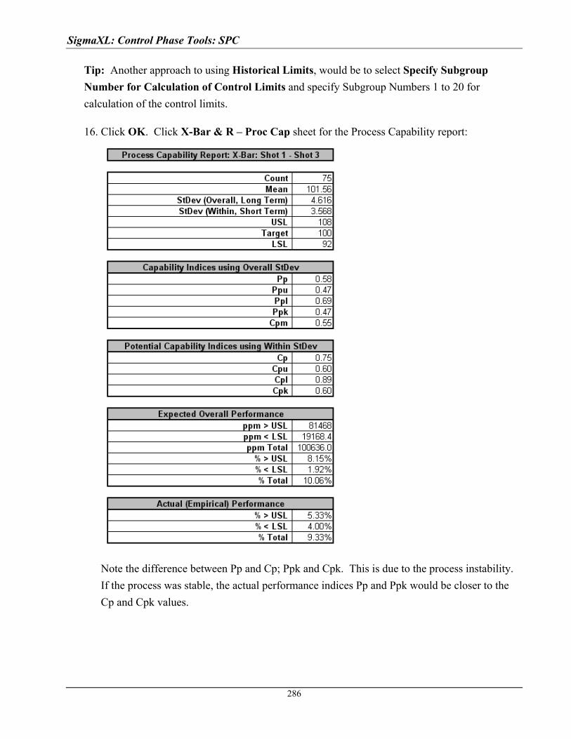
SigmaXL: Control Phase Tools: SPC
Tip: Another approach to using Historical Limits, would be to select Specify Subgroup
Number for Calculation of Control Limits and specify Subgroup Numbers 1 to 20 for
calculation of the control limits.
16. Click OK. Click X-Bar & R – Proc Cap sheet for the Process Capability report:
Note the difference between Pp and Cp; Ppk and Cpk. This is due to the process instability.
If the process was stable, the actual performance indices Pp and Ppk would be closer to the
Cp and Cpk values.
286
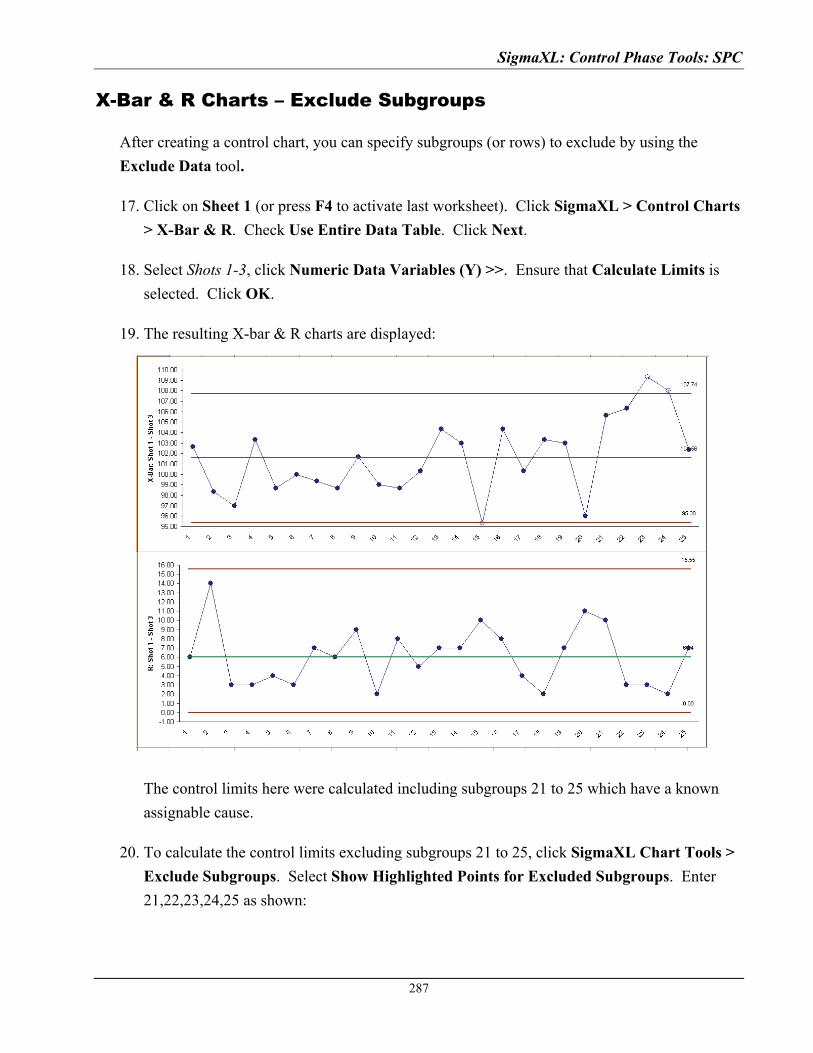
SigmaXL: Control Phase Tools: SPC
287
X-Bar & R Charts – Exclude Subgroups
After creating a control chart, you can specify subgroups (or rows) to exclude by using the
Exclude Data tool.
17. Click on Sheet 1 (or press F4 to activate last worksheet). Click SigmaXL > Control Charts
> X-Bar & R. Check Use Entire Data Table. Click Next.
18. Select Shots 1-3, click Numeric Data Variables (Y) >>. Ensure that Calculate Limits is
selected. Click OK.
19. The resulting X-bar & R charts are displayed:
The control limits here were calculated including subgroups 21 to 25 which have a known
assignable cause.
20. To calculate the control limits excluding subgroups 21 to 25, click SigmaXL Chart Tools >
Exclude Subgroups. Select Show Highlighted Points for Excluded Subgroups. Enter
21,22,23,24,25 as shown:

SigmaXL: Control Phase Tools: SPC
21. Click Exclude Subgroups. The control chart limits are recalculated and the excluded points
are highlighted:
Tip: You can also choose to show gaps for excluded subgroups or delete excluded subgroups
from the charts.
288
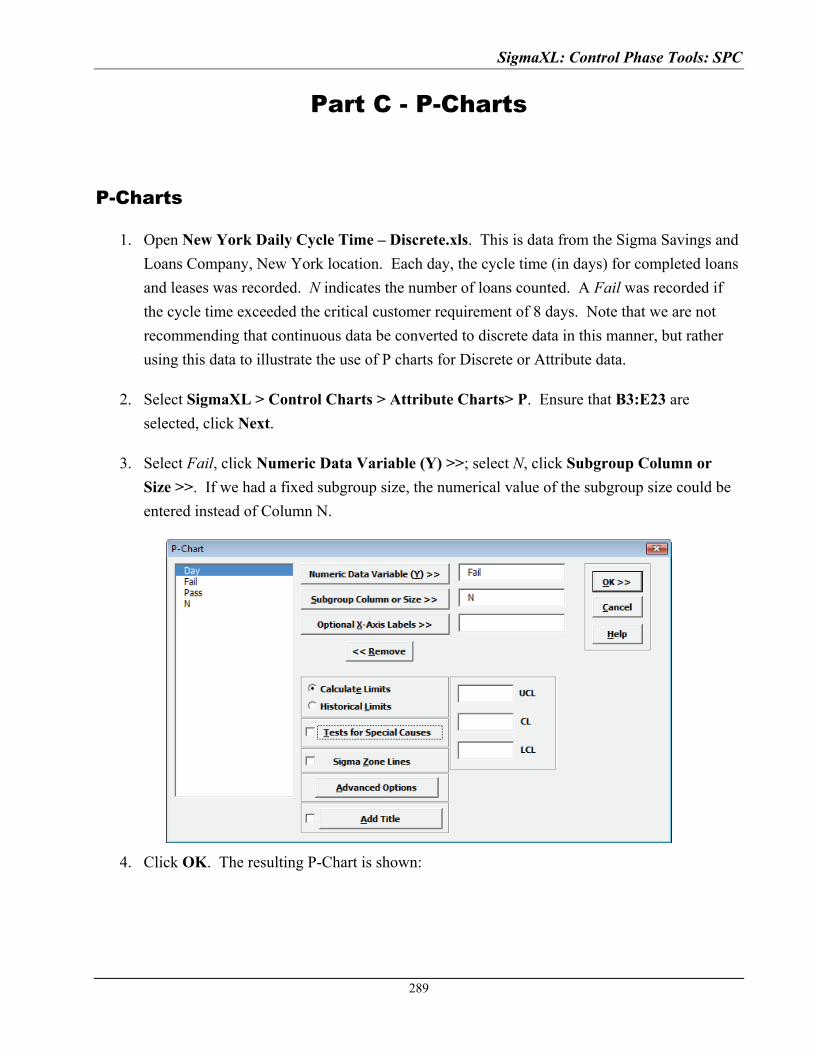
SigmaXL: Control Phase Tools: SPC
289
Part C - P-Charts
P-Charts
1. Open New York Daily Cycle Time – Discrete.xls. This is data from the Sigma Savings and
Loans Company, New York location. Each day, the cycle time (in days) for completed loans
and leases was recorded. N indicates the number of loans counted. A Fail was recorded if
the cycle time exceeded the critical customer requirement of 8 days. Note that we are not
recommending that continuous data be converted to discrete data in this manner, but rather
using this data to illustrate the use of P charts for Discrete or Attribute data.
2. Select SigmaXL > Control Charts > Attribute Charts> P. Ensure that B3:E23 are
selected, click Next.
3. Select Fail, click Numeric Data Variable (Y) >>; select N, click Subgroup Column or
Size >>. If we had a fixed subgroup size, the numerical value of the subgroup size could be
entered instead of Column N.
4. Click OK. The resulting P-Chart is shown:
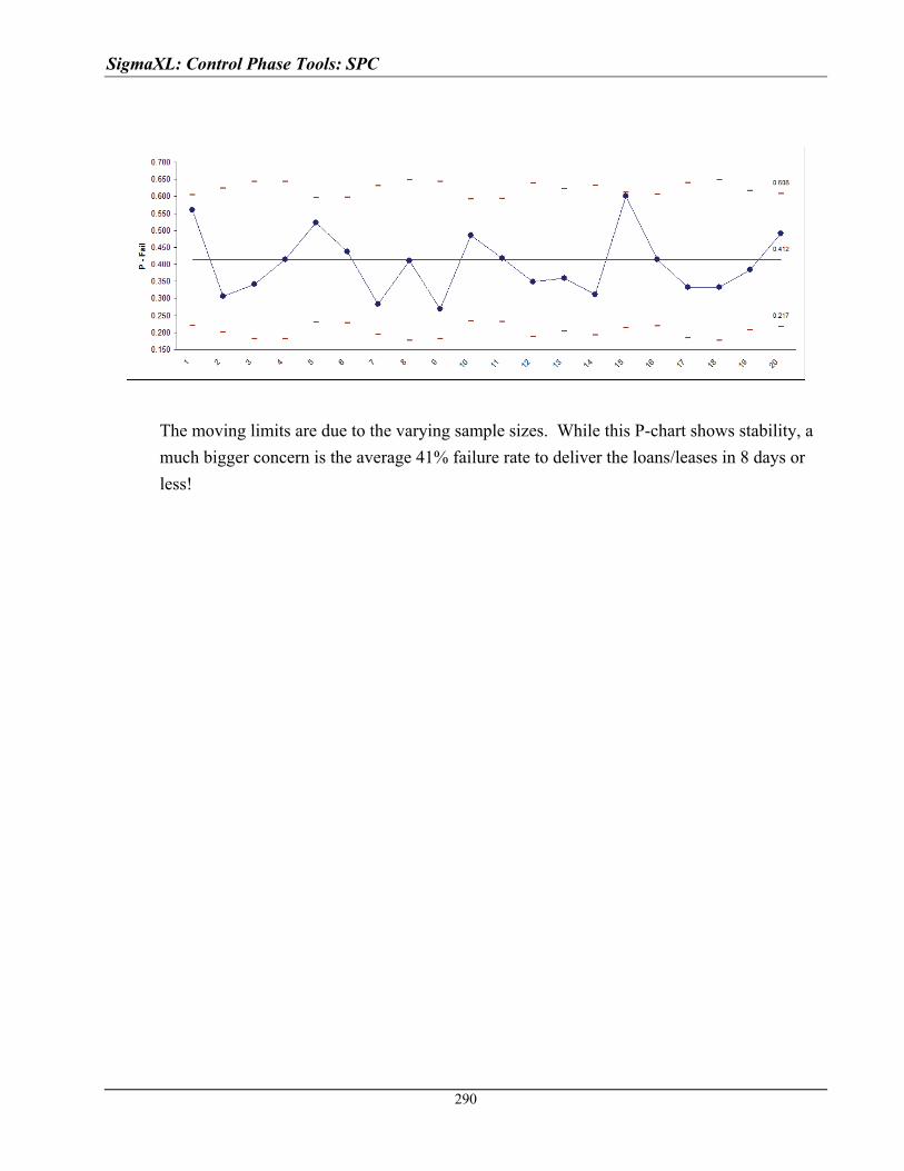
SigmaXL: Control Phase Tools: SPC
The moving limits are due to the varying sample sizes. While this P-chart shows stability, a
much bigger concern is the average 41% failure rate to deliver the loans/leases in 8 days or
less!
290
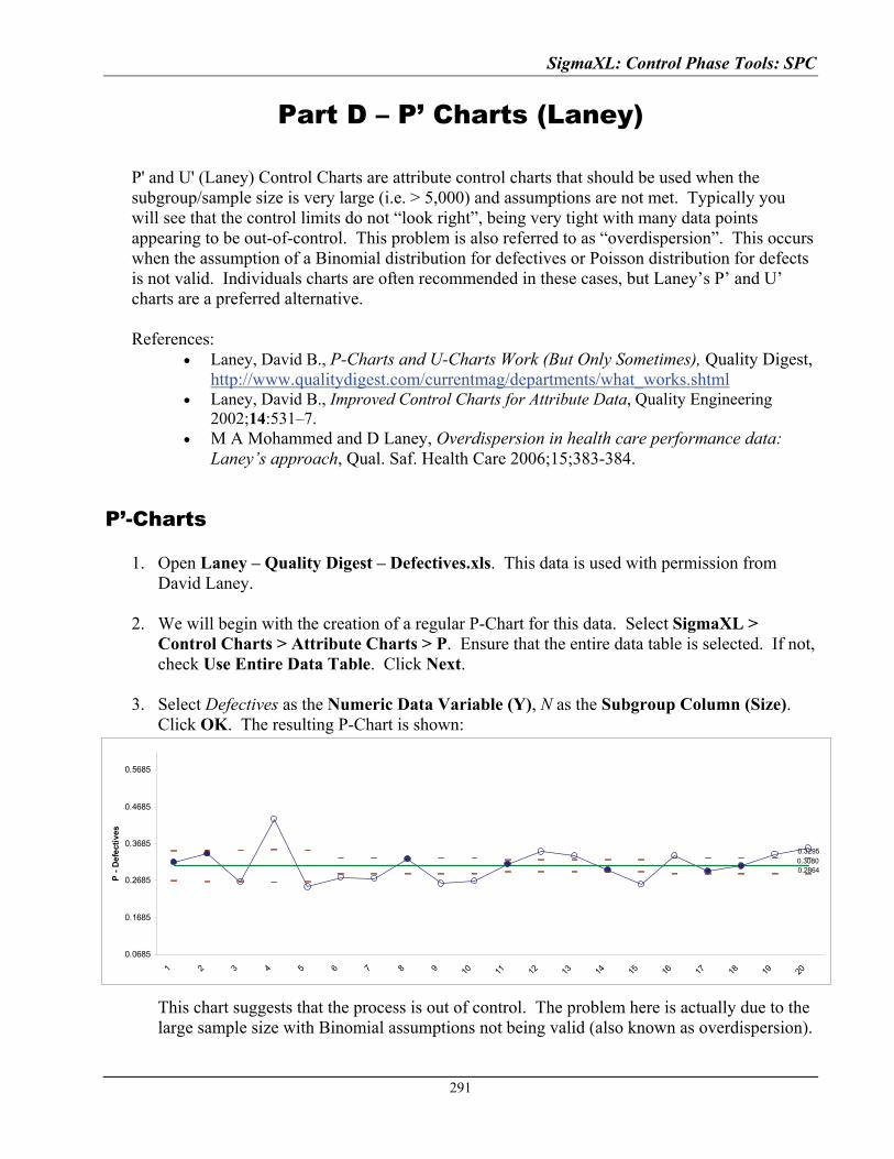
SigmaXL: Control Phase Tools: SPC
291
Part D – P’ Charts (Laney)
P' and U' (Laney) Control Charts are attribute control charts that should be used when the subgroup/sample size is very large (i.e. > 5,000) and assumptions are not met. Typically you will see that the control limits do not “look right”, being very tight with many data points appearing to be out-of-control. This problem is also referred to as “overdispersion”. This occurs when the assumption of a Binomial distribution for defectives or Poisson distribution for defects is not valid. Individuals charts are often recommended in these cases, but Laney’s P’ and U’ charts are a preferred alternative. References:
Laney, David B., P-Charts and U-Charts Work (But Only Sometimes), Quality Digest, http://www.qualitydigest.com/currentmag/departments/what_works.shtml
Laney, David B., Improved Control Charts for Attribute Data, Quality Engineering 2002;14:531–7.
M A Mohammed and D Laney, Overdispersion in health care performance data: Laney’s approach, Qual. Saf. Health Care 2006;15;383-384.
P’-Charts
1. Open Laney – Quality Digest – Defectives.xls. This data is used with permission from David Laney.
2. We will begin with the creation of a regular P-Chart for this data. Select SigmaXL > Control Charts > Attribute Charts > P. Ensure that the entire data table is selected. If not, check Use Entire Data Table. Click Next.
3. Select Defectives as the Numeric Data Variable (Y), N as the Subgroup Column (Size). Click OK. The resulting P-Chart is shown: This chart suggests that the process is out of control. The problem here is actually due to the large sample size with Binomial assumptions not being valid (also known as overdispersion).
0.30800.2864
0.3295
0.0685
0.1685
0.2685
0.3685
0.4685
0.5685
1 2 3 4 5 6 7 8 9 10 11 12 13 14 15 16 17 18 19 20
P -
Def
ecti
ves
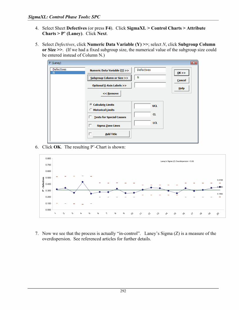
SigmaXL: Control Phase Tools: SPC
4. Select Sheet Defectives (or press F4). Click SigmaXL > Control Charts > Attribute Charts > P’ (Laney). Click Next.
5. Select Defectives, click Numeric Data Variable (Y) >>; select N, click Subgroup Column or Size >>. (If we had a fixed subgroup size, the numerical value of the subgroup size could be entered instead of Column N.)
6. Click OK. The resulting P’-Chart is shown:
0.3080
0.1992
0.4168
0.000
0.100
0.200
0.300
0.400
0.500
0.600
0.700
0.800
1 2 3 4 5 6 7 8 9 10 11 12 13 14 15 16 17 18 19 20
P' -
Def
ecti
ves
Laney's Sigma (Z) Overdispersion = 5.06
7. Now we see that the process is actually “in-control”. Laney’s Sigma (Z) is a measure of the overdispersion. See referenced articles for further details.
292
SigmaXL: Control Phase Tools: SPC
293
Part E – Control Chart Selection Tool
The Control Chart Selection Tool makes it easy for you to select the correct statistical process
control chart depending on data type and subgroup/sample type and size.
Data Types and Definitions
Continuous/Variable: Data that is measured on a continuous scale where a mid-point (or other
subdivision) has meaning. For example, when measuring cycle time, 2.5 days has meaning.
Other examples include distance, weight, thickness, length and cost. Customer Satisfaction on a
1 to 5 scale can be considered as continuous in that a satisfaction score of 3.5 has meaning.
Continuous data is always in numeric format.
Discrete/Attribute: Data that is categorical in nature. If we have defect types 1, 2, and 3, defect
type 1.5 has no meaning. Other examples of discrete data would be customer complaints and
reasons for product return. Discrete data can be text or integer numeric format.
Defective: An entire unit that is nonconforming to customer requirements. A unit may be
defective because of one or more defects. For example, an application form is good only if all
critical entry fields are correct. Any error in a critical field is a defect, resulting in a defective
form. A single form can have more than one defect.
Defect: Any specific nonconformity to customer requirements. There can be more than one
defect per unit or area of opportunity, such as the entry errors described above.
Subgroup/Sample: Data for a subgroup are usually collected within a short period of time to
ensure homogeneous conditions within the subgroup (common cause variation), in order to
detect differences between subgroups (special cause variation).
Subgroup/Sample Size: The number of observations within your sample, not the number of
samples. Subgroup sizes of 3 to 5 are common for continuous measures in parts manufacturing,
while individual measurements are common in chemical processes (temperature, pH) and
transactional areas (financial). Subgroup size for discrete data should be a minimum of 50.
Subgroup/Sample Size is constant: The number of observations within your sample remains
fixed over time.

SigmaXL: Control Phase Tools: SPC
Subgroup/Sample Size varies: The number of observations within your sample varies over
time.
Subgroup/Sample Size is very large and assumptions not met: This applies to discrete data
when the subgroup sizes are approximately 5,000 or higher and the control limits do not “look
right,” being very tight with many data points appearing to be out-of-control. This problem is
also referred to as “overdispersion”. This occurs when the assumption of a Binomial distribution
for defectives or Poisson distribution for defects is not valid. (Note: If the problem of
overdispersion is apparent with your continuous data, use SigmaXL > Control Charts >
Advanced Charts > I-MR-R or I-MR-S).
Control Chart Selection Tool – Individuals Chart
1. Open Customer Data.xls, click on Sheet 1. Click SigmaXL > Control Charts > Control
Chart Selection Tool.
2. We would like to create a control chart of the Overall Satisfaction data. Since this can be
considered as continuous data, the data type is Continuous/Variable Data. The
subgroup/sample size is 1 (i.e. there is no subgrouping), so select Individuals
(subgroup/sample size = 1). At this point, we can choose Individuals or Individuals and
Moving Range. We will keep the simpler Individuals selection as shown. (Note that the
above data types and definitions can be viewed by clicking the Data Types and Definitions
tab):
3. Click OK. This starts up the Individuals Chart dialog (see Part A – Individuals Charts for
continuation).
294
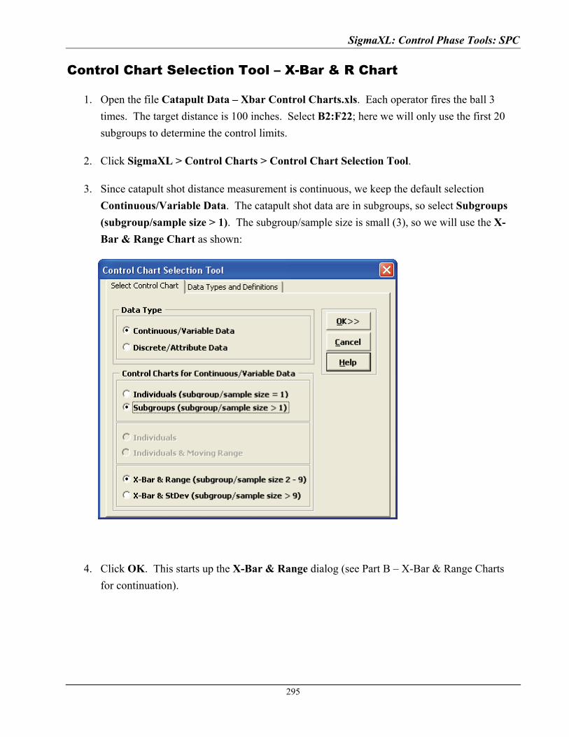
SigmaXL: Control Phase Tools: SPC
295
Control Chart Selection Tool – X-Bar & R Chart
1. Open the file Catapult Data – Xbar Control Charts.xls. Each operator fires the ball 3
times. The target distance is 100 inches. Select B2:F22; here we will only use the first 20
subgroups to determine the control limits.
2. Click SigmaXL > Control Charts > Control Chart Selection Tool.
3. Since catapult shot distance measurement is continuous, we keep the default selection
Continuous/Variable Data. The catapult shot data are in subgroups, so select Subgroups
(subgroup/sample size > 1). The subgroup/sample size is small (3), so we will use the X-
Bar & Range Chart as shown:
4. Click OK. This starts up the X-Bar & Range dialog (see Part B – X-Bar & Range Charts
for continuation).
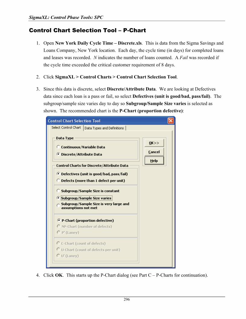
SigmaXL: Control Phase Tools: SPC
Control Chart Selection Tool – P-Chart
1. Open New York Daily Cycle Time – Discrete.xls. This is data from the Sigma Savings and
Loans Company, New York location. Each day, the cycle time (in days) for completed loans
and leases was recorded. N indicates the number of loans counted. A Fail was recorded if
the cycle time exceeded the critical customer requirement of 8 days.
2. Click SigmaXL > Control Charts > Control Chart Selection Tool.
3. Since this data is discrete, select Discrete/Attribute Data. We are looking at Defectives
data since each loan is a pass or fail, so select Defectives (unit is good/bad, pass/fail). The
subgroup/sample size varies day to day so Subgroup/Sample Size varies is selected as
shown. The recommended chart is the P-Chart (proportion defective):
4. Click OK. This starts up the P-Chart dialog (see Part C – P-Charts for continuation).
296

SigmaXL: Control Phase Tools: SPC
297
Part F – Advanced Charts: I-MR-R/S
I-MR-R Charts
If the within-subgroup variability is much smaller than between subgroup, the classical X-bar &
R (or S) chart will not work, producing numerous (false) alarms. The correct chart to use, in this
case, is the I-MR-R (or S) chart. The subgroup averages are treated as individual values (I-MR)
and the within subgroup ranges are plotted on the Range chart.
1. Open Multi-Vari Data.xls. Select Sheet Between. We saw this data previously using Multi-
Vari charts. First, we will incorrectly use the X-bar & R chart, and then apply the correct I-
MR-R chart.
2. Click SigmaXL > Control Charts > X-bar & R. Check Use Entire Data Table.
3. Click Next. Select Stacked Column Format. Select Measurement, click Numeric Data
Variable (Y) >>; select unit, click Subgroup Column or Size >>.
4. Click OK. Resulting X-bar & R chart:
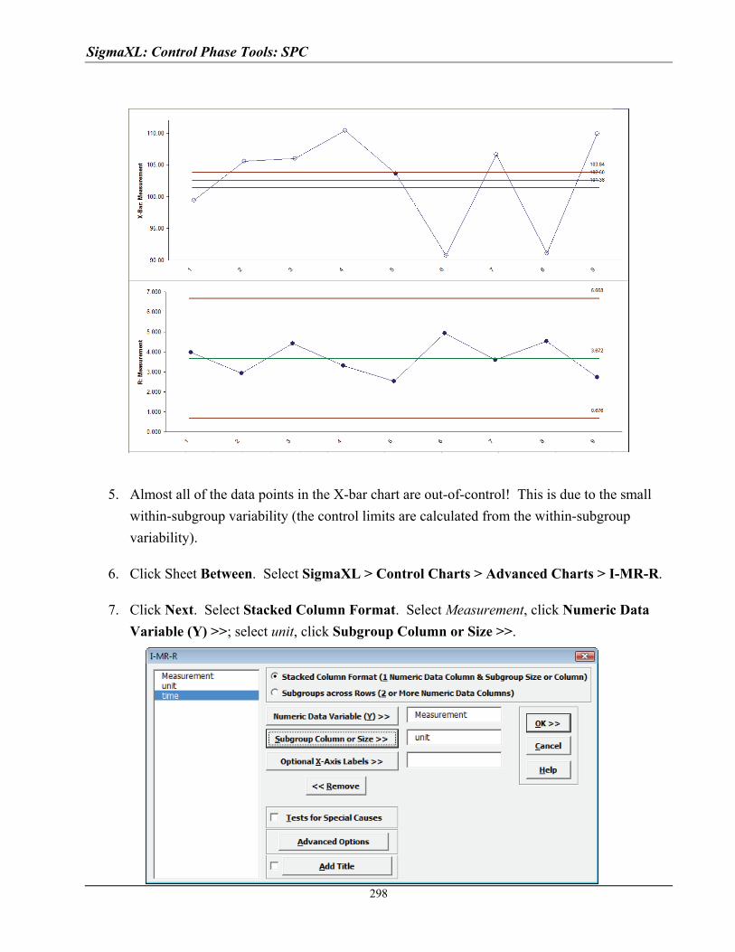
SigmaXL: Control Phase Tools: SPC
5. Almost all of the data points in the X-bar chart are out-of-control! This is due to the small
within-subgroup variability (the control limits are calculated from the within-subgroup
variability).
6. Click Sheet Between. Select SigmaXL > Control Charts > Advanced Charts > I-MR-R.
7. Click Next. Select Stacked Column Format. Select Measurement, click Numeric Data
Variable (Y) >>; select unit, click Subgroup Column or Size >>.
298
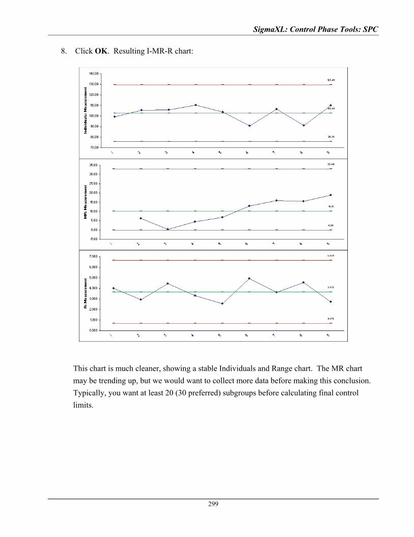
SigmaXL: Control Phase Tools: SPC
299
8. Click OK. Resulting I-MR-R chart:
This chart is much cleaner, showing a stable Individuals and Range chart. The MR chart
may be trending up, but we would want to collect more data before making this conclusion.
Typically, you want at least 20 (30 preferred) subgroups before calculating final control
limits.

Copyright © 2004-2011, SigmaXL Inc.
SigmaXL Appendix: Statistical Details for Nonnormal Distributions
and Transformations

SigmaXL: Appendix
303
Statistical Details for Nonnormal Distributions and Transformations
Maximum Likelihood Estimation (MLE)
Maximum likelihood estimates of the parameters are calculated by maximizing the likelihood
function with respect to the parameters. The likelihood function is simply the sum of the log of the
probability density function (PDF) for each uncensored observation, and the log of the complement
of the cumulative density function (CDF) for each right censored observation (in Reliability/Weibull
Analysis). Initial estimates are derived using a branch and bound algorithm.
The maximum likelihood estimates are then calculated using the Newton-Raphson method. This is
an iterative process that uses both the first and second derivatives to move to a point at which no
further improvement in the likelihood is possible.
The standard errors of the parameter estimates are derived from the Hessian matrix. This matrix,
which describes the curvature of a function, is the square matrix of second-order partial derivatives
of the function.
For some data sets, the likelihood function for threshold models is unbounded, and the maximum
likelihood methodology fails. In this context, a threshold is estimated using a bias correction
method. This is an iterative methodology that evaluates the threshold based on the difference
between the minimum value of the variate and the prediction for the minimum value, conditional on
the current values of the parameters.
References for MLE and Distributions:
Greene, W.H. Econometric Analysis 4th Ed Prentice Hall, New Jersey.
Johnson, N. L., and Kotz, S. (1990). "Use of moments in deriving distributions and some characterizations", Mathematical Scientist, Vol. 15, pp. 42-52.
Johnson, N.L., Kotz, S. and Balakrishnan, N. (1994). Continuous Univariate Distributions-Volume 1, Second Ed., Wiley, New York.
Johnson, N.L., Kotz, S. and Balakrishnan, N. (1995). Continuous Univariate Distributions-Volume 2, Second Ed., Wiley, New York.
Nocedal, J. and Wright, S.J. (1999). Numerical Optimization, Springer-Verlag, New York.
Sleeper, A. (2006). Six Sigma Distribution Modeling, McGraw-Hill, New York.
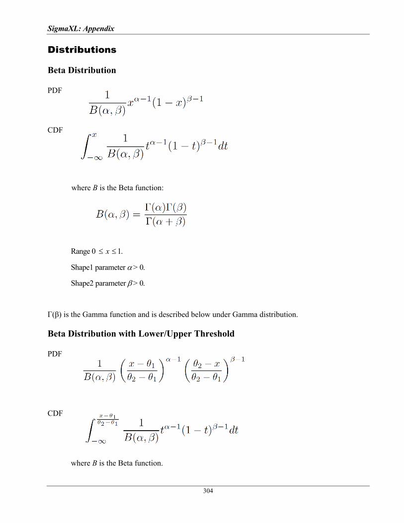
SigmaXL: Appendix
304
Distributions
Beta Distribution
CDF
where B is the Beta function:
Range 0 x 1.
Shape1 parameter > 0.
Shape2 parameter > 0.
Γ(β) is the Gamma function and is described below under Gamma distribution.
Beta Distribution with Lower/Upper Threshold
CDF
where B is the Beta function.
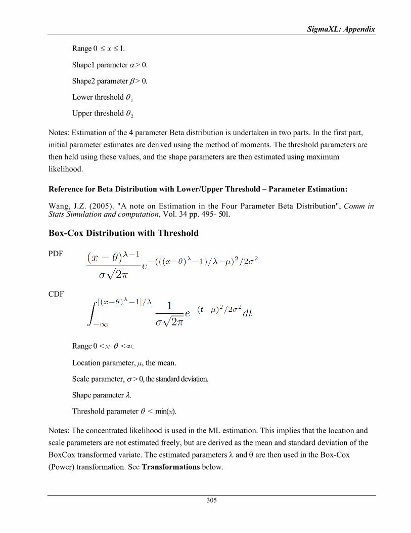
SigmaXL: Appendix
Range 0 x 1.
Shape1 parameter > 0.
Shape2 parameter > 0.
Lower threshold 1
Upper threshold 2
Notes: Estimation of the 4 parameter Beta distribution is undertaken in two parts. In the first part,
initial parameter estimates are derived using the method of moments. The threshold parameters are
then held using these values, and the shape parameters are then estimated using maximum
likelihood.
Reference for Beta Distribution with Lower/Upper Threshold – Parameter Estimation:
Wang, J.Z. (2005). "A note on Estimation in the Four Parameter Beta Distribution", Comm in Stats Simulation and computation, Vol. 34 pp. 495- 501.
Box-Cox Distribution with Threshold
305
CDF
Range < x - <.
Location parameter, µ, the mean.
Scale parameter, > 0, the standard deviation.
Shape parameter .
Threshold parameter < min(x).
Notes: The concentrated likelihood is used in the ML estimation. This implies that the location and
scale parameters are not estimated freely, but are derived as the mean and standard deviation of the
BoxCox transformed variate. The estimated parameters and are then used in the Box-Cox
(Power) transformation. See Transformations below.
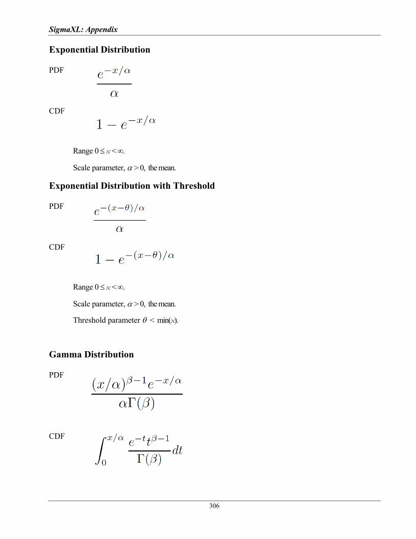
SigmaXL: Appendix
306
Exponential Distribution
CDF
Range 0 x <.
Scale parameter, > 0, the mean.
Exponential Distribution with Threshold
CDF
Range 0 x <.
Scale parameter, > 0, the mean.
Threshold parameter < min(x).
Gamma Distribution
CDF

SigmaXL: Appendix
where Γ(β) is the Gamma function:
307
Range 0 x <.
Scale parameter > 0.
Shape parameter > 0.
Gamma Distribution with Threshold
CDF
Range 0 x - <.
Scale parameter > 0.
Shape parameter > 0.
Threshold parameter < min(x).
Half Normal Distribution
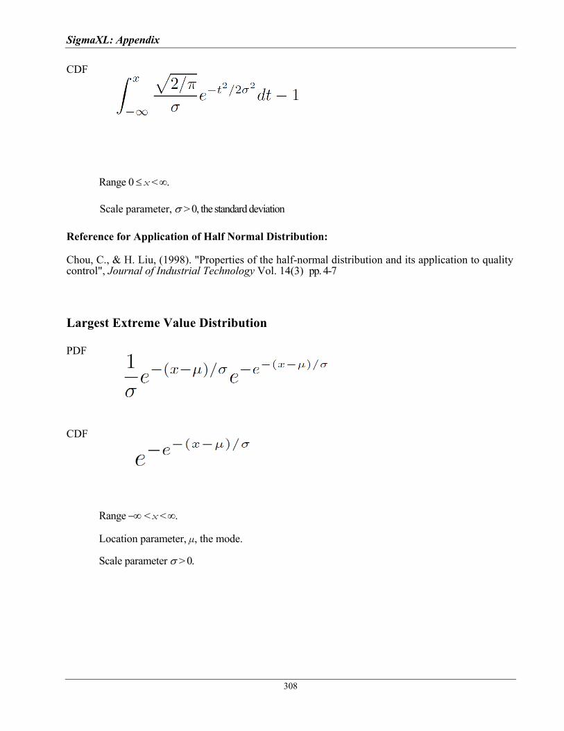
SigmaXL: Appendix
308
CDF
Range 0 x <.
Scale parameter, > 0, the standard deviation
Reference for Application of Half Normal Distribution:
Chou, C., & H. Liu, (1998). "Properties of the half-normal distribution and its application to quality control", Journal of Industrial Technology Vol. 14(3) pp. 4-7
Largest Extreme Value Distribution
CDF
Range < x <.
Location parameter, µ, the mode.
Scale parameter > 0.
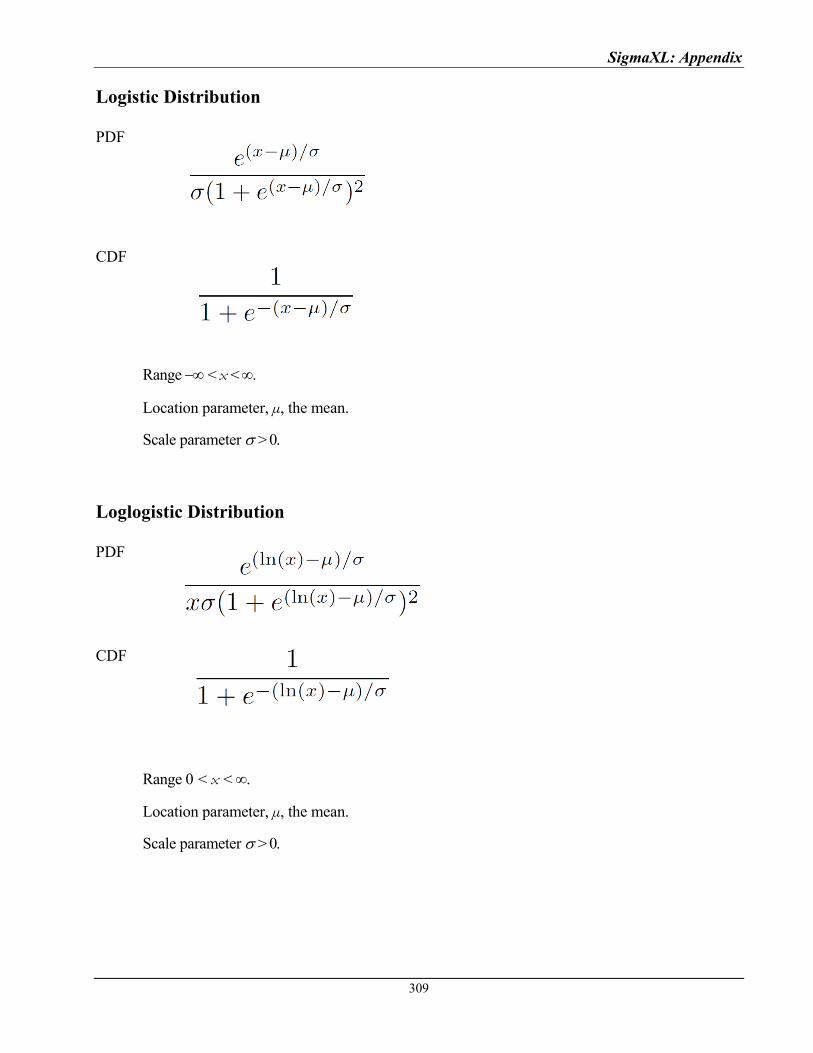
SigmaXL: Appendix
Logistic Distribution
CDF
Range < x <.
Location parameter, µ, the mean.
Scale parameter > 0.
Loglogistic Distribution
CDF
Range 0 < x <.
Location parameter, µ, the mean.
Scale parameter > 0.
309
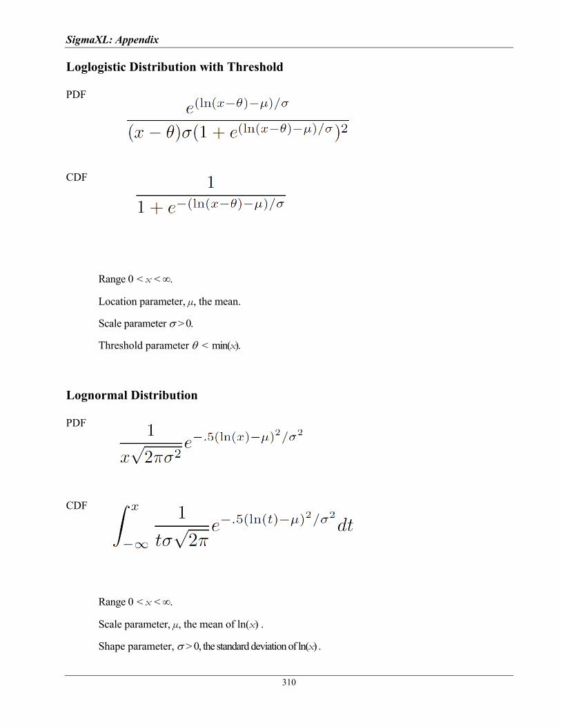
SigmaXL: Appendix
310
Loglogistic Distribution with Threshold
CDF
Range 0 < x <.
Location parameter, µ, the mean.
Scale parameter > 0.
Threshold parameter < min(x).
Lognormal Distribution
CDF
Range 0 < x <.
Scale parameter, µ, the mean of ln(x) .
Shape parameter, > 0, the standard deviation of ln(x) .
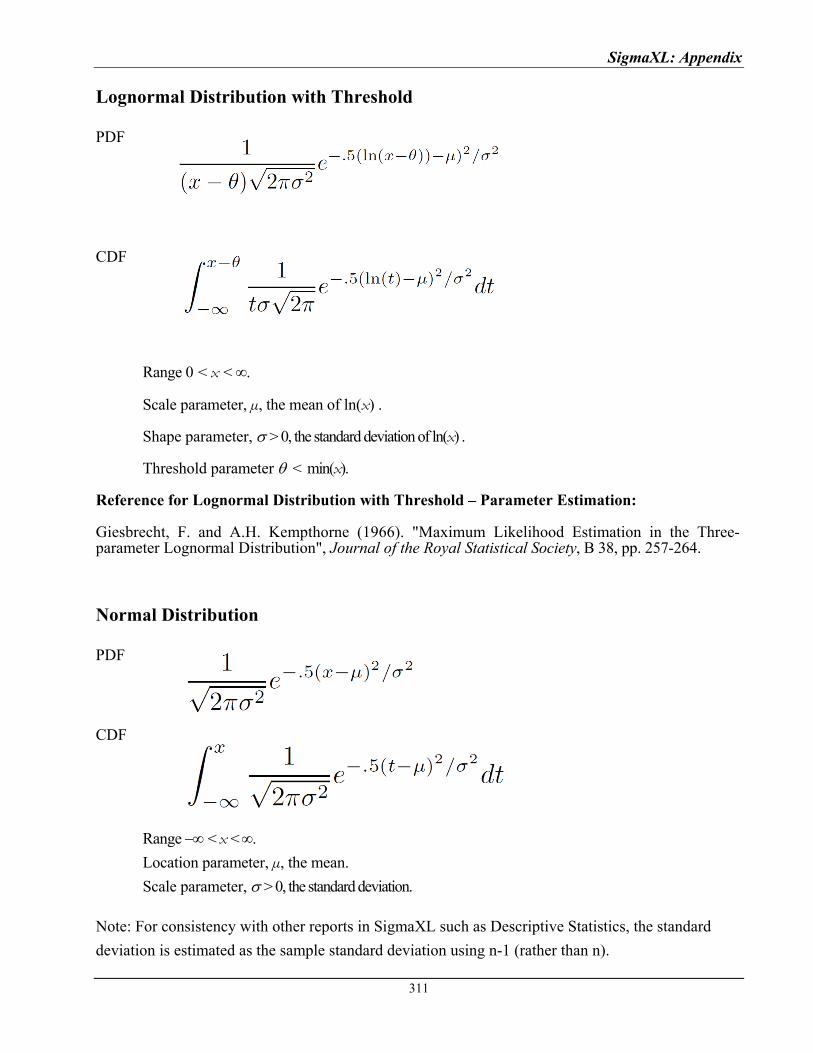
SigmaXL: Appendix
Lognormal Distribution with Threshold
CDF
Range 0 < x <.
Scale parameter, µ, the mean of ln(x) .
Shape parameter, > 0, the standard deviation of ln(x) .
Threshold parameter < min(x).
Reference for Lognormal Distribution with Threshold – Parameter Estimation:
Giesbrecht, F. and A.H. Kempthorne (1966). "Maximum Likelihood Estimation in the Three-parameter Lognormal Distribution", Journal of the Royal Statistical Society, B 38, pp. 257-264.
Normal Distribution
CDF
311
Range < x <.
Location parameter, µ, the mean.
Scale parameter, > 0, the standard deviation.
Note: For consistency with other reports in SigmaXL such as Descriptive Statistics, the standard
deviation is estimated as the sample standard deviation using n-1 (rather than n).
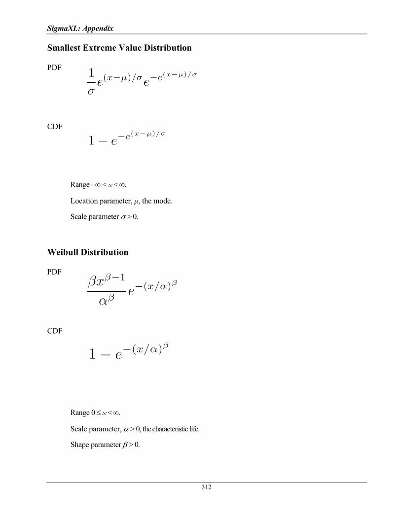
SigmaXL: Appendix
312
Smallest Extreme Value Distribution
CDF
Range < x <.
Location parameter, µ, the mode.
Scale parameter > 0.
Weibull Distribution
CDF
Range 0 x <.
Scale parameter, > 0, the characteristic life.
Shape parameter > 0.
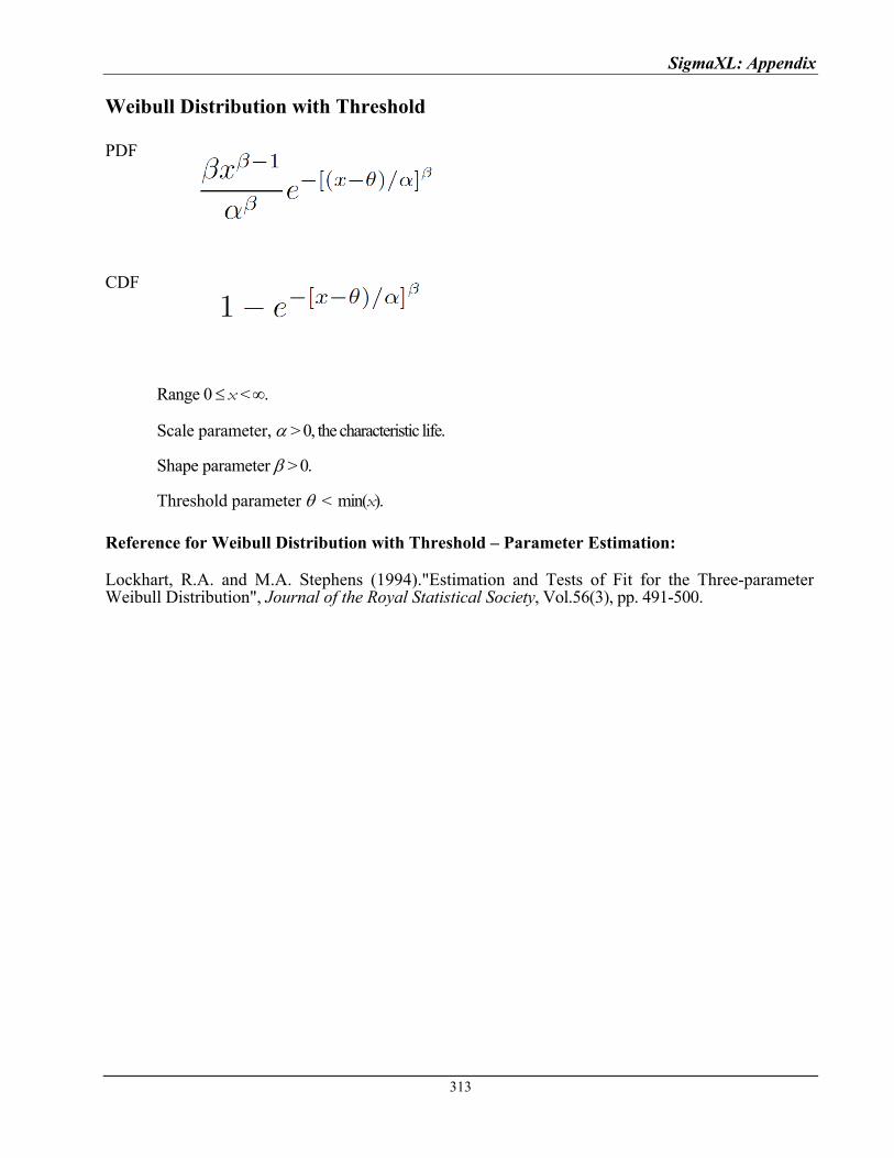
SigmaXL: Appendix
Weibull Distribution with Threshold
CDF
Range 0 x <.
Scale parameter, > 0, the characteristic life.
Shape parameter > 0.
Threshold parameter < min(x).
Reference for Weibull Distribution with Threshold – Parameter Estimation:
Lockhart, R.A. and M.A. Stephens (1994)."Estimation and Tests of Fit for the Three-parameter Weibull Distribution", Journal of the Royal Statistical Society, Vol.56(3), pp. 491-500.
313

SigmaXL: Appendix
314
Transformations
Box-Cox (Power) Transformation
. ≠ 0
. = 0
Range < x <.
Shape parameter .
Note: The optimum shape parameter,, is derived using a grid search in which the criteria function is the
standard deviation of the standardized transformed variable.
Box-Cox (Power) Transformation with Threshold
. ≠ 0
. = 0
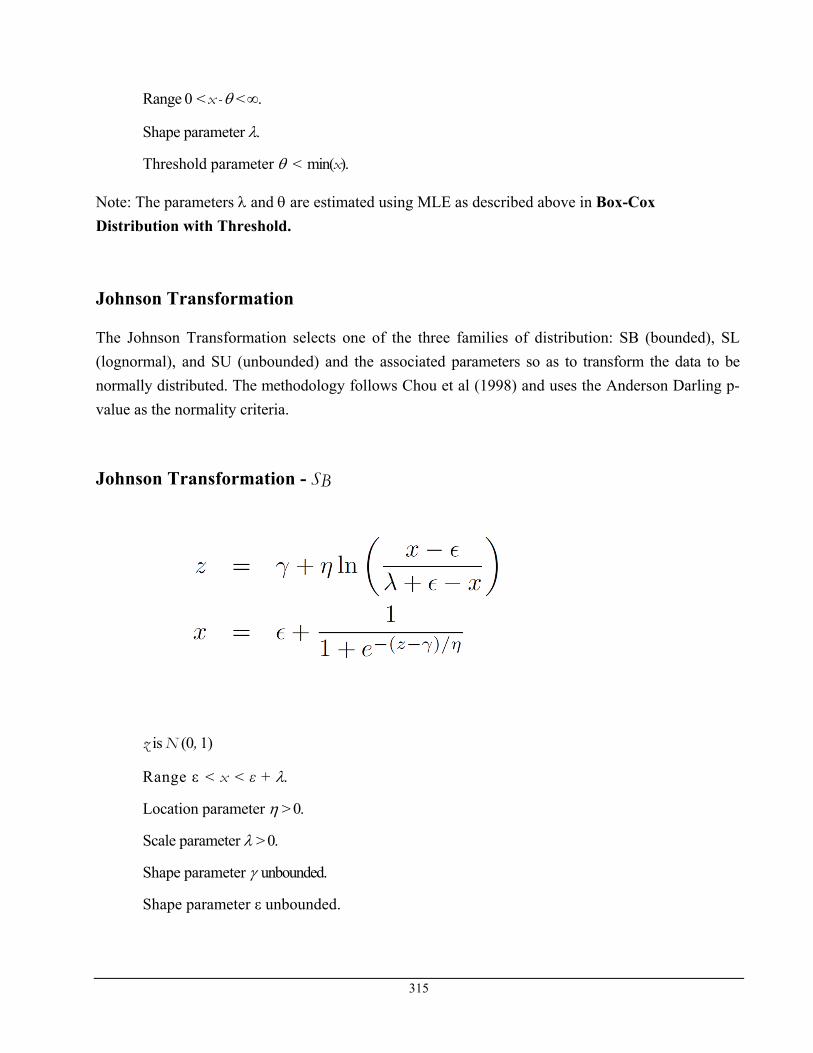
SigmaXL: Appendix
Range < x - <.
Shape parameter .
Threshold parameter < min(x).
Note: The parameters and are estimated using MLE as described above in Box-Cox
Distribution with Threshold.
Johnson Transformation
The Johnson Transformation selects one of the three families of distribution: SB (bounded), SL
(lognormal), and SU (unbounded) and the associated parameters so as to transform the data to be
normally distributed. The methodology follows Chou et al (1998) and uses the Anderson Darling p-
value as the normality criteria.
Johnson Transformation - SB
z is N (0, 1)
Range ε < x < ε + .
Location parameter > 0.
Scale parameter > 0.
Shape parameter unbounded.
Shape parameter ε unbounded.
315
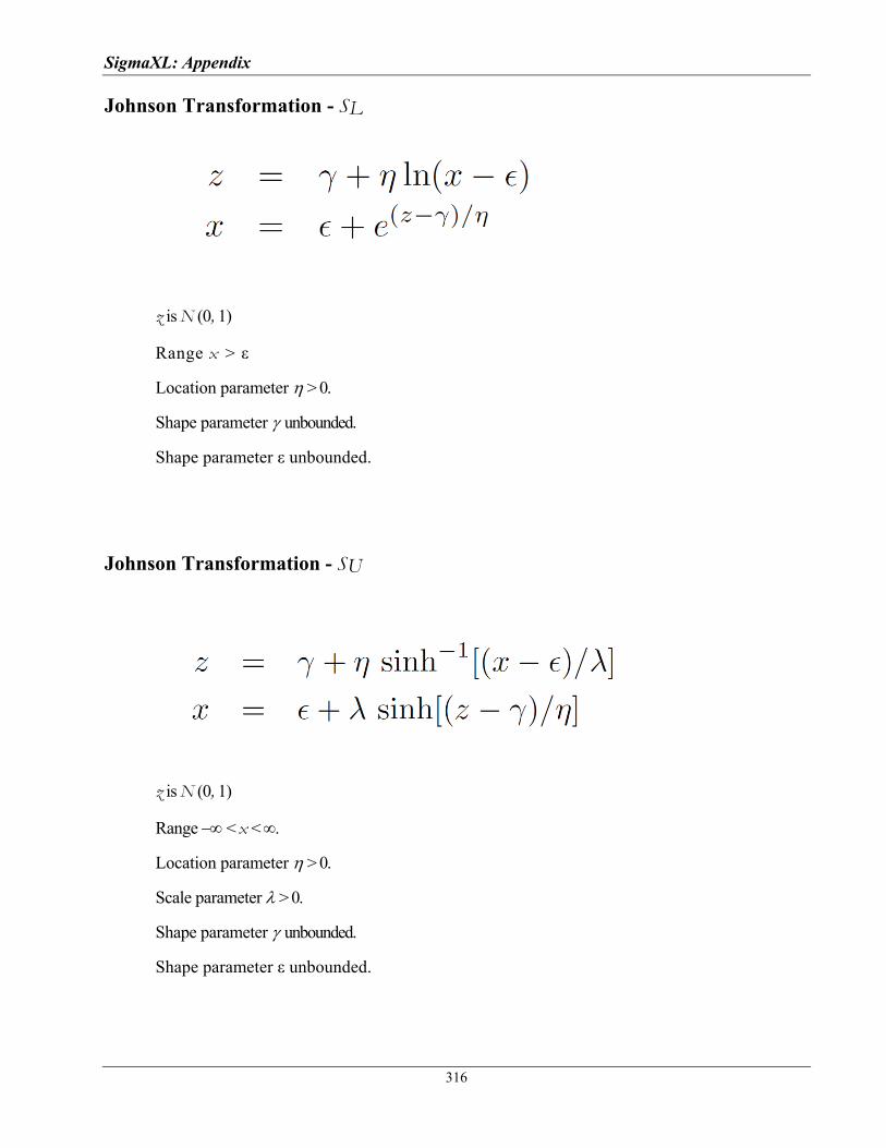
SigmaXL: Appendix
316
Johnson Transformation - SL
z is N (0, 1)
Range x > ε
Location parameter > 0.
Shape parameter unbounded.
Shape parameter ε unbounded.
Johnson Transformation - SU
z is N (0, 1)
Range < x <.
Location parameter > 0.
Scale parameter > 0.
Shape parameter unbounded.
Shape parameter ε unbounded.

SigmaXL: Appendix
317
References for Johnson Transformation:
Chou,Y., A.M. Polansky, and R.L. Mason (1998). "Transforming Non-Normal Data to Normality in Statistical Process Control," Journal of Quality Technology, Vol. 30(2), pp. 133-141.
David, H.A. (1981). Order Statistics, John Wiley & Sons, New York
Tadikamalla,P.,R. (1980). "Notes and Comments: On Simulating Non-Normal Distributions", Psychometrika,, Vol. 45(2), pp. 273-279.
Automatic Best Fit
SigmaXL uses the Anderson Darling p-value as the criteria to determine best fit. All distributions
and transformations are considered and the model with the highest AD p-value is initially selected
(denoted as adpvalmax). A search is then carried out for models that are close, having an AD p-
value greater than adpvalmax - 0.1 (with an added criteria that AD pvalue be > 0.2), but having
fewer parameters than the initial best fit model. If a simpler model is identified, then this is selected
as the best fit.
Since AD p-values are not available for distributions with thresholds (other than Weibull), an
estimate is obtained by transforming the data to normality and then using a modified Anderson
Darling Normality test on the transformed data. The transformed z-values are obtained by using the
inverse cdf of the normal distribution on the cdf of the nonnormal distribution. The Anderson
Darling Normality test assumes a mean = 0 and standard deviation = 1.
This approach, unique to SigmaXL, is an extension of the Chou methodology used in Johnson
Transformations and allows a goodness of fit comparison across all distributions and
transformations.
Another approach to comparing models is Akaike's information criterion (AIC) developed by
Hirotsugu Akaike. AIC is the MLE log-likelihood with a penalty for the number of terms in the
model (where the penalty factor also depends on the sample size, n). The AD p-value method used
by SigmaXL has the advantage that it is not limited to models with maximum likelihood parameter
estimation.
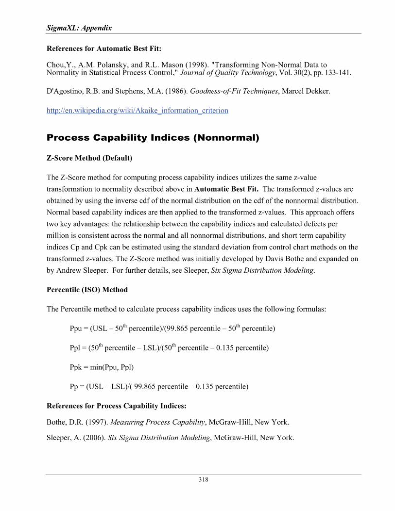
SigmaXL: Appendix
318
References for Automatic Best Fit:
Chou,Y., A.M. Polansky, and R.L. Mason (1998). "Transforming Non-Normal Data to Normality in Statistical Process Control," Journal of Quality Technology, Vol. 30(2), pp. 133-141.
D'Agostino, R.B. and Stephens, M.A. (1986). Goodness-of-Fit Techniques, Marcel Dekker.
http://en.wikipedia.org/wiki/Akaike_information_criterion
Process Capability Indices (Nonnormal)
Z-Score Method (Default)
The Z-Score method for computing process capability indices utilizes the same z-value
transformation to normality described above in Automatic Best Fit. The transformed z-values are
obtained by using the inverse cdf of the normal distribution on the cdf of the nonnormal distribution.
Normal based capability indices are then applied to the transformed z-values. This approach offers
two key advantages: the relationship between the capability indices and calculated defects per
million is consistent across the normal and all nonnormal distributions, and short term capability
indices Cp and Cpk can be estimated using the standard deviation from control chart methods on the
transformed z-values. The Z-Score method was initially developed by Davis Bothe and expanded on
by Andrew Sleeper. For further details, see Sleeper, Six Sigma Distribution Modeling.
Percentile (ISO) Method
The Percentile method to calculate process capability indices uses the following formulas:
Ppu = (USL – 50th percentile)/(99.865 percentile – 50th percentile)
Ppl = (50th percentile – LSL)/(50th percentile – 0.135 percentile)
Ppk = min(Ppu, Ppl)
Pp = (USL – LSL)/( 99.865 percentile – 0.135 percentile)
References for Process Capability Indices:
Bothe, D.R. (1997). Measuring Process Capability, McGraw-Hill, New York.
Sleeper, A. (2006). Six Sigma Distribution Modeling, McGraw-Hill, New York.
SigmaXL: Appendix
319
Control Charts (Nonnormal)
Individuals – Original Data
The Individuals – Original Data chart displays the untransformed data with control limits calculated as:
UCL = 99.865 percentile
CL = 50th percentile
LCL = 0.135 percentile
The benefit of displaying this chart is that one can observe the original untransformed data. Since
the control limits are based on percentiles, this represents the overall, long term variation rather than
the typical short term variation. The limits will likely be nonsymmetrical.
Individuals/Moving Range – Normalized Data
The Individuals/Moving Range – Normalized Data chart displays the transformed z-values with
control limits calculated using the standard Shewhart formulas for Individuals and Moving Range
charts. The benefit of using this chart is that tests for special causes can be applied and the control
limits are based on short term variation. The disadvantage is that one is observing transformed data
on the chart rather than the original data.
SigmaXL’s default setting is to display the three charts: Individuals – Original Data, Individuals &
Moving Range – Normalized Data (with tests for special causes unchecked).

SigmaXL: Appendix
320
This page is intentionally blank.