Sig Metrics 11
12
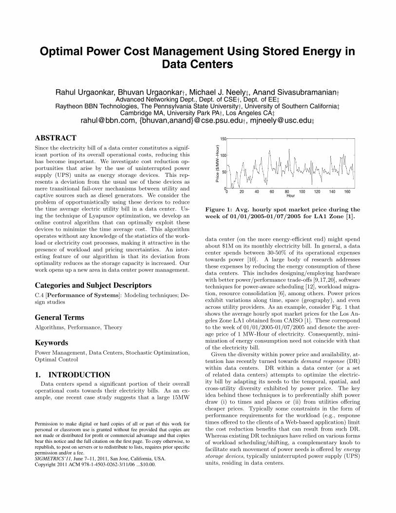
Optimal Power Cost Management Using Stored Energy in Data Centers Rahul Urgaonkar, Bhuvan Urgaonkar†, Michael J. Neely‡, Anand Sivasubramanian† Advanced Networking Dept., Dept. of CSE†, Dept. of EE‡ Raytheon BBN Technologies, The Pennsylvania State University†, University of Southern California‡ Cambridge MA, University Park PA†, Los Angeles CA‡ [email protected], {bhuvan,anand}@cse.psu.edu† , [email protected]‡ ABSTRACT Since the electricity bill of a data center constitutes a signif- icant portion of its overall operational costs, reducing this has become important. We investigate cost reduction op- portunities that arise by the use of uninterrupted power supply (UPS) units as energy storage devices. This rep- resents a deviation from the usual use of these devices as mere transitional fail-over mechanisms between utility and captive sources such as diesel generators. We consider the problem of opportunistically using these devices to reduce the time average electric utility bill in a data center. Us- ing the technique of Lyapunov optimization, we develop an online control algorithm that can optimally exploit these devices to minimize the time average cost. This algorithm operates without any knowledge of the statistics of the work- load or electricity cost processes, making it attractive in the presence of workload and pricing uncertainties. An inter- esting feature of our algorithm is that its deviation from optimality reduces as the storage capacity is increased. Our work opens up a new area in data center power management. Categories and Subject Descriptors C.4 [Performance of Systems]: Modeling techniques; De- sign studies General Terms Algorithms, Performance, Theory Keywords Power Management, Data Centers, Stochastic Optimization, Optimal Control 1. INTRODUCTION Data centers spend a significant portion of their overall operational costs towards their electricity bills. As an ex- ample, one recent case study suggests that a large 15MW Permission to make digital or hard copies of all or part of this work for personal or classroom use is granted without fee provided that copies are not made or distributed for profit or commercial advantage and that copies bear this notice and the full citation on the first page. To copy otherwise, to republish, to post on servers or to redistribute to lists, requires prior specific permission and/or a fee. SIGMETRICS’11, June 7–11, 2011, San Jose, California, USA. Copyright 2011 ACM 978-1-4503-0262-3/11/06 ...$10.00. 0 20 40 60 80 100 120 140 160 0 50 100 150 Hour Price ($/MW-Hour) Figure 1: Avg. hourly spot market price during the week of 01/01/2005-01/07/2005 for LA1 Zone [1]. data center (on the more energy-efficient end) might spend about $1M on its monthly electricity bill. In general, a data center spends between 30-50% of its operational expenses towards power [10]. A large body of research addresses these expenses by reducing the energy consumption of these data centers. This includes designing/employing hardware with better power/performance trade-offs [9,17,20], software techniques for power-aware scheduling [12], workload migra- tion, resource consolidation [6], among others. Power prices exhibit variations along time, space (geography), and even across utility providers. As an example, consider Fig. 1 that shows the average hourly spot market prices for the Los An- geles Zone LA1 obtained from CAISO [1]. These correspond to the week of 01/01/2005-01/07/2005 and denote the aver- age price of 1 MW-Hour of electricity. Consequently, mini- mization of energy consumption need not coincide with that of the electricity bill. Given the diversity within power price and availability, at- tention has recently turned towards demand response (DR) within data centers. DR within a data center (or a set of related data centers) attempts to optimize the electric- ity bill by adapting its needs to the temporal, spatial, and cross-utility diversity exhibited by power price. The key idea behind these techniques is to preferentially shift power draw (i) to times and places or (ii) from utilities offering cheaper prices. Typically some constraints in the form of performance requirements for the workload (e.g., response times offered to the clients of a Web-based application) limit the cost reduction benefits that can result from such DR. Whereas existing DR techniques have relied on various forms of workload scheduling/shifting, a complementary knob to facilitate such movement of power needs is offered by energy storage devices, typically uninterrupted power supply (UPS) units, residing in data centers.
description
ieee paper
Transcript of Sig Metrics 11
Optimal Power Cost Management Using Stored Energy inData Centers
Rahul Urgaonkar, Bhuvan Urgaonkar†, Michael J. Neely‡, Anand Sivasubramanian†Advanced Networking Dept., Dept. of CSE†, Dept. of EE‡
Raytheon BBN Technologies, The Pennsylvania State University†, University of Southern California‡Cambridge MA, University Park PA†, Los Angeles CA‡
[email protected], {bhuvan,anand}@cse.psu.edu†, [email protected]‡
ABSTRACTSince the electricity bill of a data center constitutes a signif-icant portion of its overall operational costs, reducing thishas become important. We investigate cost reduction op-portunities that arise by the use of uninterrupted powersupply (UPS) units as energy storage devices. This rep-resents a deviation from the usual use of these devices asmere transitional fail-over mechanisms between utility andcaptive sources such as diesel generators. We consider theproblem of opportunistically using these devices to reducethe time average electric utility bill in a data center. Us-ing the technique of Lyapunov optimization, we develop anonline control algorithm that can optimally exploit thesedevices to minimize the time average cost. This algorithmoperates without any knowledge of the statistics of the work-load or electricity cost processes, making it attractive in thepresence of workload and pricing uncertainties. An inter-esting feature of our algorithm is that its deviation fromoptimality reduces as the storage capacity is increased. Ourwork opens up a new area in data center power management.
Categories and Subject DescriptorsC.4 [Performance of Systems]: Modeling techniques; De-sign studies
General TermsAlgorithms, Performance, Theory
KeywordsPower Management, Data Centers, Stochastic Optimization,Optimal Control
1. INTRODUCTIONData centers spend a significant portion of their overall
operational costs towards their electricity bills. As an ex-ample, one recent case study suggests that a large 15MW
Permission to make digital or hard copies of all or part of this work forpersonal or classroom use is granted without fee provided that copies arenot made or distributed for profit or commercial advantage and that copiesbear this notice and the full citation on the first page. To copy otherwise, torepublish, to post on servers or to redistribute to lists, requires prior specificpermission and/or a fee.SIGMETRICS’11, June 7–11, 2011, San Jose, California, USA.Copyright 2011 ACM 978-1-4503-0262-3/11/06 ...$10.00.
0 20 40 60 80 100 120 140 1600
50
100
150
Hour
Price
($
/MW
−H
ou
r)
Figure 1: Avg. hourly spot market price during theweek of 01/01/2005-01/07/2005 for LA1 Zone [1].
data center (on the more energy-efficient end) might spendabout $1M on its monthly electricity bill. In general, a datacenter spends between 30-50% of its operational expensestowards power [10]. A large body of research addressesthese expenses by reducing the energy consumption of thesedata centers. This includes designing/employing hardwarewith better power/performance trade-offs [9,17,20], softwaretechniques for power-aware scheduling [12], workload migra-tion, resource consolidation [6], among others. Power pricesexhibit variations along time, space (geography), and evenacross utility providers. As an example, consider Fig. 1 thatshows the average hourly spot market prices for the Los An-geles Zone LA1 obtained from CAISO [1]. These correspondto the week of 01/01/2005-01/07/2005 and denote the aver-age price of 1 MW-Hour of electricity. Consequently, mini-mization of energy consumption need not coincide with thatof the electricity bill.
Given the diversity within power price and availability, at-tention has recently turned towards demand response (DR)within data centers. DR within a data center (or a setof related data centers) attempts to optimize the electric-ity bill by adapting its needs to the temporal, spatial, andcross-utility diversity exhibited by power price. The keyidea behind these techniques is to preferentially shift powerdraw (i) to times and places or (ii) from utilities offeringcheaper prices. Typically some constraints in the form ofperformance requirements for the workload (e.g., responsetimes offered to the clients of a Web-based application) limitthe cost reduction benefits that can result from such DR.Whereas existing DR techniques have relied on various formsof workload scheduling/shifting, a complementary knob tofacilitate such movement of power needs is offered by energystorage devices, typically uninterrupted power supply (UPS)units, residing in data centers.
A data center deploys captive power sources, typicallydiesel generators (DG), that it uses for keeping itself poweredup when the utility experiences an outage. The UPS unitsserve as a bridging mechanism to facilitate this transitionfrom utility to DG: upon a utility failure, the data center iskept powered by the UPS unit using energy stored withinits batteries, before the DG can start up and provide power.Whereas this transition takes only 10-20 seconds, UPS unitshave enough battery capacity to keep the entire data centerpowered at its maximum power needs for anywhere between5-30 minutes. Tapping into the energy reserves of the UPSunit can allow a data center to improve its electricity bill.Intuitively, the data center would store energy within theUPS unit when prices are low and use this to augment thedraw from the utility when prices are high.
In this paper, we consider the problem of developing anonline control policy to exploit the UPS unit along with thepresence of delay-tolerance within the workload to optimizethe data center’s electricity bill. This is a challenging prob-lem because data centers experience time-varying workloadsand power prices with possibly unknown statistics. Evenwhen statistics can be approximated (say by learning us-ing past observations), traditional approaches to constructoptimal control policies involve the use of Markov DecisionTheory and Dynamic Programming [5]. It is well knownthat these techniques suffer from the “curse of dimensional-ity”where the complexity of computing the optimal strategygrows with the system size. Furthermore, such solutionsresult in hard-to-implement systems, where significant re-computation might be needed when statistics change.
In this work, we make use of a different approach thatcan overcome the challenges associated with dynamic pro-gramming. This approach is based on the recently developedtechnique of Lyapunov optimization [8] [15] that enables thedesign of online control algorithms for such time-varyingsystems. These algorithms operate without requiring anyknowledge of the system statistics and are easy to imple-ment. We design such an algorithm for optimally exploitingthe UPS unit and delay-tolerance of workloads to minimizethe time average cost. We show that our algorithm can getwithin O(1/V ) of the optimal solution where the maximumvalue of V is limited by battery capacity. We note that, forthe same parameters, a dynamic programming based ap-proach (if it can be solved) will yield a better result thanour algorithm. However, this gap reduces as the battery ca-pacity is increased. Our algorithm is thus most useful whensuch scaling is practical.
2. RELATED WORKOne recent body of work proposes online algorithms for
using UPS units for cost reduction via shaving workload“peaks” that correspond to higher energy prices [3, 4]. Thiswork is highly complementary to ours in that it offers aworst-case competitive ratio analysis while our approachlooks at the average case performance. Whereas a varietyof work has looked at workload shifting for power cost re-duction [20] or other reasons such as performance and avail-ability [6], our work differs both due to its usage of energystorage as well as the cost optimality guarantees offered byour technique. Some research has considered consumers withaccess to multiple utility providers, each with a different car-bon profile, power price and availability and looked at opti-mizing cost subject to performance and/or carbon emissions
Battery
Data Center
-
+Grid
P(t) R(t) D(t)
P(t) - R(t)
W(t)
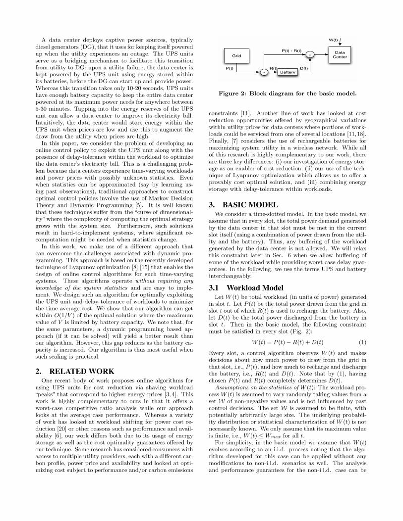
Figure 2: Block diagram for the basic model.
constraints [11]. Another line of work has looked at costreduction opportunities offered by geographical variationswithin utility prices for data centers where portions of work-loads could be serviced from one of several locations [11,18].Finally, [7] considers the use of rechargeable batteries formaximizing system utility in a wireless network. While allof this research is highly complementary to our work, thereare three key differences: (i) our investigation of energy stor-age as an enabler of cost reduction, (ii) our use of the tech-nique of Lyapunov optimization which allows us to offer aprovably cost optimal solution, and (iii) combining energystorage with delay-tolerance within workloads.
3. BASIC MODELWe consider a time-slotted model. In the basic model, we
assume that in every slot, the total power demand generatedby the data center in that slot must be met in the currentslot itself (using a combination of power drawn from the util-ity and the battery). Thus, any buffering of the workloadgenerated by the data center is not allowed. We will relaxthis constraint later in Sec. 6 when we allow buffering ofsome of the workload while providing worst case delay guar-antees. In the following, we use the terms UPS and batteryinterchangeably.
3.1 Workload ModelLet W (t) be total workload (in units of power) generated
in slot t. Let P (t) be the total power drawn from the grid inslot t out of which R(t) is used to recharge the battery. Also,let D(t) be the total power discharged from the battery inslot t. Then in the basic model, the following constraintmust be satisfied in every slot (Fig. 2):
W (t) = P (t) − R(t) + D(t) (1)
Every slot, a control algorithm observes W (t) and makesdecisions about how much power to draw from the grid inthat slot, i.e., P (t), and how much to recharge and dischargethe battery, i.e., R(t) and D(t). Note that by (1), havingchosen P (t) and R(t) completely determines D(t).
Assumptions on the statistics of W (t): The workload pro-cess W (t) is assumed to vary randomly taking values from aset W of non-negative values and is not influenced by pastcontrol decisions. The set W is assumed to be finite, withpotentially arbitrarily large size. The underlying probabil-ity distribution or statistical characterization of W (t) is notnecessarily known. We only assume that its maximum valueis finite, i.e., W (t) ≤ Wmax for all t.
For simplicity, in the basic model we assume that W (t)evolves according to an i.i.d. process noting that the algo-rithm developed for this case can be applied without anymodifications to non-i.i.d. scenarios as well. The analysisand performance guarantees for the non-i.i.d. case can be

obtained using the delayed Lyapunov drift and T slot drifttechniques developed in [8] [15].
3.2 Battery ModelIdeally, we would like to incorporate the following id-
iosyncrasies of battery operation into our model. First,batteries become unreliable as they are charged/discharged,with higher depth-of-discharge (DoD) - percentage of max-imum charge removed during a discharge cycle - causingfaster degradation in their reliability. This dependence be-tween the useful lifetime of a battery and how it is dis-charged/charged is expressed via battery lifetime charts [13].For example, with lead-acid batteries that are commonlyused in UPS units, 20% DoD yields 1400 cycles [2]. Sec-ond, batteries have conversion loss whereby a portion of theenergy stored in them is lost when discharging them (e.g.,about 10-15% for lead-acid batteries). Furthermore, cer-tain regions of battery operation (high rate of discharge)are more inefficient than others. Finally, the storage itselfmaybe“leaky”, so that the stored energy decreases over time,even in the absence of any discharging.
For simplicity, in the basic model we will assume thatthere is no power loss either in recharging or dischargingthe batteries, noting that this can be easily generalized tothe case where a fraction of R(t),D(t) is lost. We will alsoassume that the batteries are not leaky, so that the storedenergy level decreases only when they are discharged. Thisis a reasonable assumption when the time scale over whichthe loss takes place is much larger than that of interest to us.To model the effect of repeated recharging and dischargingon the battery’s lifetime, we assume that with each rechargeand discharge operation, a fixed cost (in dollars) of Crc andCdc respectively is incurred. The choice of these parameterswould affect the trade-off between the cost of the batteryitself and the cost reduction benefits it offers. For example,suppose a new battery costs B dollars and it can sustainN discharge/charge cycles (ignoring DoD for now). Thensetting Crc = Cdc = B/N would amount to expecting thebattery to “pay for itself” by augmenting the utility N timesover its lifetime.
In any slot, we assume that one can either recharge ordischarge the battery or do neither, but not both. Thismeans that for all t, we have:
R(t) > 0 =⇒ D(t) = 0, D(t) > 0 =⇒ R(t) = 0 (2)
Let Y (t) denote the battery energy level in slot t. Then, thedynamics of Y (t) can be expressed as:
Y (t + 1) = Y (t) − D(t) + R(t) (3)
The battery is assumed to have a finite capacity Ymax sothat Y (t) ≤ Ymax for all t. Further, for the purpose of relia-bility, it may be required to ensure that a minimum energylevel Ymin ≥ 0 is maintained at all times. For example, thiscould represent the amount of energy required to supportthe data center operations until a secondary power source(such as DG) is activated in the event of a grid outage.Recall that the UPS unit is integral to the availability ofpower supply to the data center upon utility outage. Indis-criminate discharging of UPS can leave the data center insituations where it is unable to safely fail-over to DG upona utility outage. Therefore, discharging the UPS must bedone carefully so that it still possesses enough charge so re-liably carry out its role as a transition device between utility
and DG. Thus, the following condition must be met in everyslot under any feasible control algorithm:
Ymin ≤ Y (t) ≤ Ymax (4)
The effectiveness of the online control algorithm we presentin Sec. 5 will depend on the magnitude of the differenceYmax − Ymin. In most practical scenarios of interest, thisvalue is expected to be at least moderately large: recentwork suggests that storing energy Ymin to last about a minuteis sufficient to offer reliable data center operation [14], whileYmax can vary between 5-20 minutes (or even higher) dueto reasons such as UPS units being available only in certainsizes and the need to keep room for future IT growth. Fur-thermore, the UPS units are sized based on the maximumprovisioned capacity of the data center, which is itself oftensubstantially (up to twice [10]) higher than the maximumactual power demand.
The initial charge level in the battery is given by Yinit andsatisfies Ymin ≤ Yinit ≤ Ymax. Finally, we assume that themaximum amounts by which we can recharge or dischargethe battery in any slot are bounded. Thus, we have ∀t:
0 ≤ R(t) ≤ Rmax, 0 ≤ D(t) ≤ Dmax (5)
We will assume that Ymax − Ymin > Rmax + Dmax whilenoting that in practice, Ymax − Ymin is much larger thanRmax + Dmax. Note that any feasible control decision onR(t),D(t) must ensure that both of the constraints (4) and(5) are satisfied. This is equivalent to the following:
0 ≤ R(t) ≤ min[Rmax, Ymax − Y (t)] (6)
0 ≤ D(t) ≤ min[Dmax, Y (t) − Ymin] (7)
3.3 Cost ModelThe cost per unit of power drawn from the grid in slot t
is denoted by C(t). In general, it can depend on both P (t),the total amount of power drawn in slot t, and an auxiliarystate variable S(t), that captures parameters such as timeof day, identity of the utility provider, etc. For example,the per unit cost may be higher during business hours, etc.Similarly, for any fixed S(t), it may be the case that C(t)increases with P (t) so that per unit cost of electricity in-creases as more power is drawn. This may be because theutility provider wants to discourage heavier loading on thegrid. Thus, we assume that C(t) is a function of both S(t)and P (t) and we denote this as:
C(t) = C(S(t), P (t)) (8)
For notational convenience, we will use C(t) to denote theper unit cost in the rest of the paper noting that the depen-dence of C(t) on S(t) and P (t) is implicit.
The auxiliary state process S(t) is assumed to evolve inde-pendently of the decisions taken by any control policy. Forsimplicity, we assume that every slot it takes values from afinite but arbitrarily large set S in an i.i.d. fashion accord-ing to a potentially unknown distribution. This can againbe generalized to non i.i.d. Markov modulated scenarios us-ing the techniques developed in [8] [15]. For each S(t), theunit cost is assumed to be a non-decreasing function of P (t).Note that it is not necessarily convex or strictly monotonicor continuous. This is quite general and can be used tomodel a variety of scenarios. A special case is when C(t) isonly a function of S(t). The optimal control action for this
case has a particularly simple form and we will highlight thisin Sec. 5.1.1. The unit cost is assumed to be non-negativeand finite for all S(t), P (t).
We assume that the maximum amount of power that canbe drawn from the grid in any slot is upper bounded byPpeak. Thus, we have for all t:
0 ≤ P (t) ≤ Ppeak (9)
Note that if we consider the original scenario where batteriesare not used, then Ppeak must be such that all workload canbe satisfied. Therefore, Ppeak ≥ Wmax.
Finally, let Cmax and Cmin denote the maximum and min-imum per unit cost respectively over all S(t), P (t). Also letχmin > 0 be a constant such that for any P1, P2 ∈ [0, Ppeak]where P1 ≤ P2, the following holds for all χ ≥ χmin:
P1(−χ + C(P1, S)) ≥ P2(−χ + C(P2, S)) ∀S ∈ S (10)
For example, when C(t) does not depend on P (t), thenχmin = Cmax satisfies (10). This follows by noting that(−Cmax + C(t)) ≤ 0 for all t. Similarly, suppose C(t)does not depend on S(t), but is continuous, convex, andincreasing in P (t). Then, it can be shown that χmin =C(Ppeak) + PpeakC′(Ppeak) satisfies (10) where C′(Ppeak)denotes the derivative of C(t) evaluated at Ppeak. In thefollowing, we assume that such a finite χmin exists for thegiven cost model. We further assume that χmin > Cmin.The case of χmin = Cmin corresponds to the degeneratecase where the unit cost is fixed for all times and we do notconsider it in this paper.
What is known in each slot? : We assume that the valueof S(t) and the form of the function C(P (t), S(t)) for thatslot is known. For example, this may be obtained before-hand using pre-advertised prices by the utility provider. Weassume that given an S(t) = s, C(t) is a deterministic func-tion of P (t) and this holds for all s. Similarly, the amount ofincoming workload W (t) is known at the beginning of eachslot.
Given this model, our goal is to design a control algorithmthat minimizes the time average cost while meeting all theconstraints. This is formalized in the next section.
4. CONTROL OBJECTIVELet P (t),R(t) and D(t) denote the control decisions made
in slot t by any feasible policy under the basic model asdiscussed in Sec. 3. These must satisfy the constraints (1),(2), (6), (7), and (9) every slot. We define the followingindicator variables that are functions of the control decisionsregarding a recharge or discharge operation in slot t:
1R(t) =
j1 if R(t) > 00 else
1D(t) =
j1 if D(t) > 00 else
Note that by (2), at most one of 1R(t) and 1C(t) can takethe value 1. Then the total cost incurred in slot t is givenby P (t)C(t) + 1R(t)Crc + 1D(t)Cdc. The time-average costunder this policy is given by:
limt→∞
1
t
t−1Xτ=0
E {P (τ )C(τ ) + 1R(τ )Crc + 1D(τ )Cdc} (11)
where the expectation above is with respect to the potentialrandomness of the control policy. Assuming for the time be-ing that this limit exists, our goal is to design a control algo-
rithm that minimizes this time average cost subject to theconstraints described in the basic model. Mathematically,this can be stated as the following stochastic optimizationproblem:
P1 :
Minimize: limt→∞
1
t
t−1Xτ=0
E {P (τ )C(τ ) + 1R(τ )Crc + 1D(τ )Cdc}
Subject to: Constraints (1), (2), (6), (7), (9)
The finite capacity and underflow constraints (6), (7) makethis a particularly challenging problem to solve even if thestatistical descriptions of the workload and unit cost processare known. For example, the traditional approach basedon Dynamic Programming [5] would have to compute theoptimal control action for all possible combinations of thebattery charge level and the system state (S(t), W (t)). In-stead, we take an alternate approach based on the techniqueof Lyapunov optimization, taking the finite size queues con-straint explicitly into account.
Note that a solution to the problem P1 is a control policythat determines the sequence of feasible control decisionsP (t), R(t), D(t), to be used. Let φopt denote the value ofthe objective in problem P1 under an optimal control policy.Define the time-average rate of recharge and discharge underany policy as follows:
R = limt→∞
1
t
t−1Xτ=0
E {R(τ )} , D = limt→∞
1
t
t−1Xτ=0
E {D(τ )} (12)
Now consider the following problem:
P2 :
Minimize: limt→∞
1
t
t−1Xτ=0
E {P (τ )C(τ ) + 1R(τ )Crc + 1D(τ )Cdc}
Subject to: Constraints (1), (2), (5), (9)
R = D (13)
Let φ denote the value of the objective in problem P2 underan optimal control policy. By comparing P1 and P2, it canbe shown that P2 is less constrained than P1. Specifically,any feasible solution to P1 would also satisfy P2. To seethis, consider any policy that satisfies (6) and (7) for all t.This ensures that constraints (4) and (5) are always metby this policy. Then summing equation (3) over all τ ∈{0, 1, 2, . . . , t − 1} under this policy and taking expectationof both sides yields:
E {Y (t)} − Yinit =t−1Xτ=0
E {R(τ ) − D(τ )}
Since Ymin ≤ Y (t) ≤ Ymax for all t, dividing both sidesby t and taking limits as t → ∞ yields R = D. Thus,this policy satisfies constraint (13) of P2. Therefore, anyfeasible solution to P1 also satisfies P2. This implies thatthe optimal value of P2 cannot exceed that of P1, so thatφ ≤ φopt.
Our approach to solving P1 will be based on this obser-vation. We first note that it is easier to characterize theoptimal solution to P2. This is because the dependence onY (t) has been removed. Specifically, it can be shown thatthe optimal solution to P2 can be achieved by a station-

ary, randomized control policy that chooses control actionsP (t), D(t), R(t) every slot purely as a function (possibly ran-domized) of the current state (W (t), S(t)) and independentof the battery charge level Y (t). This fact is presented inthe following lemma:
Lemma 1. (Optimal Stationary, Randomized Policy): Ifthe workload process W (t) and auxiliary process S(t) arei.i.d. over slots, then there exists a stationary, randomizedpolicy that takes control decisions P stat(t), Rstat(t), Dstat(t)every slot purely as a function (possibly randomized) of thecurrent state (W (t), S(t)) while satisfying the constraints(1), (2), (5), (9) and providing the following guarantees:
E˘Rstat(t)
¯= E
˘Dstat(t)
¯(14)
E˘P stat(t)C(t) + 1stat
R (t)Crc + 1statD (t)Cdc
¯= φ (15)
where the expectations above are with respect to the station-ary distribution of (W (t), S(t)) and the randomized controldecisions.
Proof. This result follows from the framework in [8,15]and is omitted for brevity.
It should be noted that while it is possible to characterizeand potentially compute such a policy, it may not be feasi-ble for the original problem P1 as it could violate the con-straints (6) and (7). However, the existence of such a policycan be used to construct an approximately optimal policythat meets all the constraints of P1 using the technique ofLyapunov optimization [8] [15]. This policy is dynamic anddoes not require knowledge of the statistical description ofthe workload and cost processes. We present this policy andderive its performance guarantees in the next section. Thisdynamic policy is approximately optimal where the approx-imation factor improves as the battery capacity increases.Also note that the distance from optimality for our policy ismeasured in terms of φ. However, since φ ≤ φopt, in prac-tice, the approximation factor is better than the analyticalbounds.
5. OPTIMAL CONTROL ALGORITHMWe now present an online control algorithm that approx-
imately solves P1. This algorithm uses a control parameterV > 0 that affects the distance from optimality as shownlater. This algorithm also makes use of a “queueing” statevariable X(t) to track the battery charge level and is definedas follows:
X(t) = Y (t) − V χmin − Dmax − Ymin (16)
Recall that Y (t) denotes the actual battery charge level inslot t and evolves according to (3). It can be seen that X(t)is simply a shifted version of Y (t) and its dynamics is givenby:
X(t + 1) = X(t) − D(t) + R(t) (17)
Note that X(t) can be negative. We will show that this def-inition enables our algorithm to ensure that the constraint(4) is met.
We are now ready to state the dynamic control algorithm.Let (W (t), S(t)) and X(t) denote the system state in slot t.Then the dynamic algorithm chooses control action P (t) as
Wmid
Wlow
Whigh
t
Figure 3: Periodic W (t) process in the example.
the solution to the following optimization problem:
P3 :
Minimize: X(t)P (t) + VhP (t)C(t) + 1R(t)Crc + 1D(t)Cdc
i
Subject to: Constraints (1), (2), (5), (9)
The constraints above result in the following constraint onP (t):
Plow ≤ P (t) ≤ Phigh (18)
wherePlow = max[0, W (t)−Dmax] and Phigh = min[Ppeak, W (t)+Rmax]. Let P ∗(t), R∗(t), and D∗(t) denote the optimal so-lution to P3. Then, the dynamic algorithm chooses therecharge and discharge values as follows.
R∗(t) =
jP ∗(t) − W (t) if P ∗(t) > W (t)0 else
D∗(t) =
jW (t) − P ∗(t) if P ∗(t) < W (t)0 else
Note that if P ∗(t) = W (t), then both R∗(t) = 0 and D∗(t) =0 and all demand is met using power drawn from the grid. Itcan be seen from the above that the control decisions satisfythe constraints 0 ≤ R∗(t) ≤ Rmax and 0 ≤ D∗(t) ≤ Dmax.That the finite battery constraints and the constraints (6),(7) are also met will be shown in Sec. 5.3.
After computing these quantities, the algorithm imple-ments them and updates the queueing variable X(t) accord-ing to (17). This process is repeated every slot. Note thatin solving P3, the control algorithm only makes use of thecurrent system state values and does not require knowledgeof the statistics of the workload or unit cost processes. Thus,it is myopic and greedy in nature. From P3, it is seen thatthe algorithm tries to recharge the battery when X(t) isnegative and per unit cost is low. And it tries to dischargethe battery when X(t) is positive. That this is sufficient toachieve optimality will be shown in Theorem 1. The queue-ing variable X(t) plays a crucial role as making decisionspurely based on prices is not necessarily optimal.
To get some intuition behind the working of this algo-rithm, consider the following simple example. Suppose W (t)can take three possible values from the set {Wlow, Wmid, Whigh}where Wlow < Wmid < Whigh. Similarly, C(t) can take threepossible values in {Clow, Cmid, Chigh} where Clow < Cmid <Chigh and does not depend on P (t). We assume that theworkload process evolves in a frame-based periodic fashion.Specifically, in every odd numbered frame, W (t) = Wmid
for all except the last slot of the frame when W (t) = Wlow.In every even numbered frame, W (t) = Wmid for all exceptthe last slot of the frame when W (t) = Whigh. This is il-
Ymax 20 30 40 50 75 100V 0 1.25 2.5 3.75 6.875 10.0
Avg. Cost 94.0 92.5 91.1 88.5 88.0 87.0
Table 1: Average Cost vs. Ymax
lustrated in Fig. 3. The C(t) process evolves similarly, suchthat C(t) = Clow when W (t) = Wlow, C(t) = Cmid whenW (t) = Wmid, and C(t) = Chigh when W (t) = Whigh.
In the following, we assume a frame size of 5 slots withWlow = 10, Wmid = 15, and Whigh = 20 units. Also, Clow =2, Cmid = 6, and Chigh = 10 dollars. Finally, Rmax =Dmax = 10, Ppeak = 20, Crc = Cdc = 5, Yinit = Ymin =0 and we vary Ymax > Rmax + Dmax. In this example,intuitively, an optimal algorithm that knows the workloadand unit cost process beforehand would recharge the batteryas much as possible when C(t) = Clow and discharge it asmuch as possible when C(t) = Chigh. In fact, it can beshown that the following strategy is feasible and achievesminimum average cost:
• If C(t) = Clow, W (t) = Wlow, then P (t) = Wlow +Rmax, R(t) = Rmax, D(t) = 0.
• If C(t) = Cmid, W (t) = Wmid, then P (t) = Wmid,R(t) = 0, D(t) = 0.
• If C(t) = Chigh, W (t) = Whigh, then P (t) = Whigh −Dmax, R(t) = 0, D(t) = Dmax.
The time average cost resulting from this strategy can beeasily calculated and is given by 87.0 dollars/slot for allYmax > 10. Also, we note that the cost resulting from analgorithm that does not use the battery in this example isgiven by 94.0 dollars/slot.
Now we simulate the dynamic algorithm for this exam-ple for different values of Ymax for 1000 slots (200 frames).The value of V is chosen to be Ymax−Ymin−Rmax−Dmax
Chigh−Clow=
Ymax−208
(this choice will become clear in Sec. 5.2 when werelate V to the battery capacity). Note that the number ofslots for which a fully charged battery can sustain the datacenter at maximum load is Ymax/Whigh.
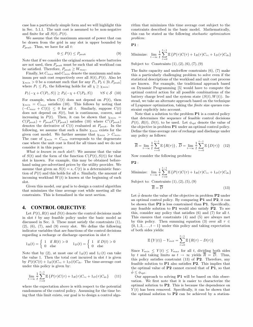
In Table 1, we show the time average cost achieved for dif-ferent values of Ymax. It can be seen that as Ymax increases,the time average cost approaches the optimal value (thisbehavior will be formalized in Theorem 1). This is remark-able given that the dynamic algorithm operates without anyknowledge of the future workload and cost processes. To ex-amine the behavior of the dynamic algorithm in more detail,we fix Ymax = 100 and look at the sample paths of the con-trol decisions taken by the optimal offline algorithm and thedynamic algorithm during the first 200 slots. This is shownin Figs. 4 and 5. It can be seen that initially, the dynamictends to perform suboptimally. But eventually it learns tomake close to optimal decisions.
It might be tempting to conclude from this example thatan algorithm based on a price threshold is optimal. Specif-ically, such an algorithm makes a recharge vs. dischargedecision depending on whether the current price C(t) issmaller or larger than a threshold. However, it is easyto construct examples where the dynamic algorithm out-performs such a threshold based algorithm. Specifically,suppose that the W (t) process takes values from the inter-val [10, 90] uniformly at random every slot. Also, suppose
0 20 40 60 80 100 120 140 160 180 20010
15
20
time
P(t
)
Figure 4: P (t) under the offline optimal solution withYmax = 100.
0 20 40 60 80 100 120 140 160 180 20010
15
20
time
P(t
)
Figure 5: P (t) under the Dynamic Algorithm withYmax = 100.
C(t) takes values from the set {2, 6, 10} dollars uniformlyat random every slot. We fix the other parameters as fol-lows: Rmax = Dmax = 10, Ppeak = 90, Crc = Cdc = 1,Yinit = Ymin = 0 and Ymax = 100. We then simulate athreshold based algorithm for different values of the thresh-old in the set {2, 6, 10} and select the one that yields thesmallest cost. This was found to be 280.7 dollars/slot. Wethen simulate the dynamic algorithm for 10000 slots withV = Ymax−20
10−2= 10.0 and it yields an average cost of 275.5
dollars/slot. We also note that the cost resulting from analgorithm that does not use the battery in this example isgiven by 300.73 dollars/slot.
We now establish two properties of the structure of theoptimal solution to P3 that will be useful in analyzing itsperformance later.
Lemma 2. The optimal solution to P3 has the followingproperties:
1. If X(t) > −V Cmin, then the optimal solution alwayschooses R∗(t) = 0.
2. If X(t) < −V χmin, then the optimal solution alwayschooses D∗(t) = 0.
Proof. See [19].
5.1 Solving P3
In general, the complexity of solving P3 depends on thestructure of the unit cost function C(t). For many casesof practical interest, P3 is easy to solve and admits closedform solutions that can be implemented in real time. Weconsider two such cases here. Let θ(t) denote the value ofthe objective in P3 when there is no recharge or discharge.Thus θ(t) = W (t)(X(t) + V C(t)).
5.1.1 C(t) does not depend on P (t)
Suppose that C(t) depends only on S(t) and not on P (t).We can rewrite the expression in the objective of P3 as
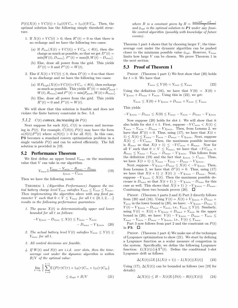
P (t)(X(t) + V C(t)) + 1R(t)V Crc + 1D(t)V Cdc. Then, theoptimal solution has the following simple threshold struc-ture.
1. If X(t) + V C(t) > 0, then R∗(t) = 0 so that there isno recharge and we have the following two cases:
(a) If Plow(X(t) + V C(t)) + V Cdc < θ(t), then dis-charge as much as possible, so that we get D∗(t) =min[W (t), Dmax], P ∗(t) = max[0, W (t) − Dmax].
(b) Else, draw all power from the grid. This yieldsD∗(t) = 0 and P ∗(t) = W (t).
2. Else if X(t)+V C(t) ≤ 0, then D∗(t) = 0 so that thereis no discharge and we have the following two cases:
(a) If Phigh(X(t)+V C(t))+V Crc < θ(t), then rechargeas much as possible. This yields R∗(t) = min[Ppeak−W (t),Rmax] and P ∗(t) = min[Ppeak, W (t)+Rmax].
(b) Else, draw all power from the grid. This yieldsR∗(t) = 0 and P ∗(t) = W (t).
We will show that this solution is feasible and does notviolate the finite battery constraint in Sec. 5.3.
5.1.2 C(t) convex, increasing in P (t)
Next suppose for each S(t), C(t) is convex and increas-
ing in P (t). For example, C(S(t), P (t)) may have the formα(S(t))P 2(t) where α(S(t)) > 0 for all S(t). In this case,P3 becomes a standard convex optimization problem in asingle variable P (t) and can be solved efficiently. The fullsolution is provided in [19].
5.2 Performance TheoremWe first define an upper bound Vmax on the maximum
value that V can take in our algorithm.
Vmax�=
Ymax − Ymin − Rmax − Dmax
χmin − Cmin(19)
Then we have the following result.
Theorem 1. (Algorithm Performance) Suppose the ini-tial battery charge level Yinit satisfies Ymin ≤ Yinit ≤ Ymax.Then implementing the algorithm above with any fixed pa-rameter V such that 0 < V ≤ Vmax for all t ∈ {0, 1, 2, . . .}results in the following performance guarantees:
1. The queue X(t) is deterministically upper and lowerbounded for all t as follows:
−V χmin − Dmax ≤ X(t) ≤ Ymax − Ymin
− Dmax − V χmin (20)
2. The actual battery level Y (t) satisfies Ymin ≤ Y (t) ≤Ymax for all t.
3. All control decisions are feasible.
4. If W (t) and S(t) are i.i.d. over slots, then the time-average cost under the dynamic algorithm is withinB/V of the optimal value:
limt→∞
1
t
t−1Xτ=0
E {P (τ )C(τ ) + 1R(τ )Crc + 1D(τ )Cdc}
≤ φopt + B/V (21)
where B is a constant given by B =max[R2
max,D2max]
2and φopt is the optimal solution to P1 under any feasi-ble control algorithm (possibly with knowledge of futureevents).
Theorem 1 part 4 shows that by choosing larger V , the time-average cost under the dynamic algorithm can be pushedcloser to the minimum possible value φopt. However, Vmax
limits how large V can be chosen. We prove Theorem 1 inthe next section.
5.3 Proof of Theorem 1Proof. (Theorem 1 part 1) We first show that (20) holds
for t = 0. We have that
Ymin ≤ Y (0) = Yinit ≤ Ymax (22)
Using the definition (16), we have that Y (0) = X(0) +V χmin + Dmax + Ymin. Using this in (22), we get:
Ymin ≤ X(0) + V χmin + Dmax + Ymin ≤ Ymax
This yields
−V χmin − Dmax ≤ X(0) ≤ Ymax − Ymin − Dmax − V χmin
Now suppose (20) holds for slot t. We will show that italso holds for slot t + 1. First, suppose −V Cmin < X(t) ≤Ymax − Ymin − Dmax − V χmin. Then, from Lemma 2, wehave that R∗(t) = 0. Thus, using (17), we have that X(t +1) ≤ X(t) ≤ Ymax − Ymin − Dmax − V χmin. Next, supposeX(t) ≤ −V Cmin. Then, the maximum possible increaseis Rmax so that X(t + 1) ≤ −V Cmin + Rmax. Now forall V such that 0 < V ≤ Vmax, we have that −V Cmin +Rmax ≤ Ymax − Ymin − Dmax − V χmin. This follows fromthe definition (19) and the fact that χmin > Cmin. Thus,we have X(t + 1) ≤ Ymax − Ymin − Dmax − V χmin.
Next, suppose −V χmin−Dmax ≤ X(t) < −V χmin. Then,from Lemma 2, we have that D∗(t) = 0. Thus, using (17)we have that X(t + 1) ≥ X(t) ≥ −V χmin − Dmax. Next,suppose −V χmin ≤ X(t). Then the maximum possible de-crease is Dmax so that X(t + 1) ≥ −V χmin −Dmax for thiscase as well. This shows that X(t + 1) ≥ −V χmin − Dmax.Combining these two bounds proves (20).
Proof. (Theorem 1 parts 2 and 3) Part 2 directly followsfrom (20) and (16). Using Y (t) = X(t) + V χmin + Dmax +Ymin in the lower bound in (20), we have: −V χmin−Dmax ≤Y (t) − V χmin − Dmax − Ymin, i.e., Ymin ≤ Y (t). Similarly,using Y (t) = X(t) + V χmin + Dmax + Ymin in the upperbound in (20), we have: Y (t) − V χmin − Dmax − Ymin ≤Ymax − Ymin − Dmax − V χmin, i.e., Y (t) ≤ Ymax.
Part 3 now follows from part 2 and the constraint on P (t)in P3.
Proof. (Theorem 1 part 4) We make use of the techniqueof Lyapunov optimization to show (21). We start by defininga Lyapunov function as a scalar measure of congestion inthe system. Specifically, we define the following Lyapunovfunction: L(X(t))�
=12X2(t). Define the conditional 1-slot
Lyapunov drift as follows:
Δ(X(t))�=E {L(X(t + 1)) − L(X(t))|X(t)} (23)
Using (17), Δ(X(t)) can be bounded as follows (see [19] fordetails):
Δ(X(t)) ≤ B − X(t)E {D(t) − R(t)|X(t)} (24)
where B =max[R2
max,D2max]
2. Following the Lyapunov opti-
mization framework of [8], we add to both sides of (24) thepenalty term V E {P (t)C(t) + 1R(t)Crc + 1D(t)Cdc|X(t)} toget the following:
Δ(X(t)) + V E {P (t)C(t) + 1R(t)Crc + 1D(t)Cdc|X(t)}≤ B − X(t)E {D(t) − R(t)|X(t)}+ V E {P (t)C(t) + 1R(t)Crc + 1D(t)Cdc|X(t)} (25)
Using (1), we can rewrite the above as:
Δ(X(t)) + V E {P (t)C(t) + 1R(t)Crc + 1D(t)Cdc|X(t)} ≤B − X(t)E {W (t)|X(t)}+ X(t)E {P (t)|X(t)}+ V E {P (t)C(t) + 1R(t)Crc + 1D(t)Cdc|X(t)} (26)
Comparing this with P3, it can be seen that given any queuevalue X(t), our control algorithm is designed to minimizethe right hand side of (26) over all possible feasible controlpolicies. This includes the optimal, stationary, randomizedpolicy given in Lemma 1. Then, plugging the control de-cisions corresponding to the stationary, randomized policy,the following holds for the dynamic algorithm:
Δ(X(t)) + V E {P (t)C(t) + 1R(t)Crc + 1D(t)Cdc|X(t)} ≤B + V E
˘P stat(t)Cstat(t) + 1stat
R (t)Crc + 1statD (t)Cdc|X(t)
¯= B + V φ ≤ B + V φopt
Taking the expectation of both sides and using the law ofiterated expectations and summing over t ∈ {0, 1, 2, . . . , T −1}, we get:
T−1Xt=0
V E {P (t)C(t) + 1R(t)Crc + 1D(t)Cdc} ≤
BT + V Tφopt − E {L(X(T ))}+ E {L(X(0))}Dividing both sides by V T and taking limit as T → ∞yields:
limT→∞
1
T
T−1Xt=0
E {P (t)C(t) + 1R(t)Crc + 1D(t)Cdc} ≤ φopt + B/V
where we have used the fact that E {L(X(0))} is finite andthat E {L(X(T ))} is non-negative.
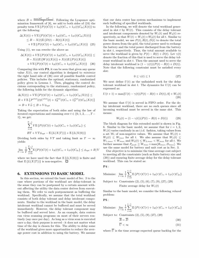
6. EXTENSIONS TO BASIC MODELIn this section, we extend the basic model of Sec. 3 to the
case where portions of the workload are delay-tolerant inthe sense they can be postponed by a certain amount with-out affecting the utility the data center derives from execut-ing them. We refer to such postponement as buffering theworkload. Specifically, we assume that the total workloadconsists of both delay tolerant and delay intolerant compo-nents. Similar to the workload in the basic model, the delayintolerant workload cannot be buffered and must be servedimmediately. However, the delay tolerant component maybe buffered and served later. As an example, data centersrun virus scanning programs on most of their servers rou-tinely (say once per day). As long as a virus scan is executedonce a day, their purpose is served - it does not matter whattime of the day is chosen for this. The ability to delay someof the workload gives more opportunities to reduce the aver-age power cost in addition to using the battery. We assume
that our data center has system mechanisms to implementsuch buffering of specified workloads.
In the following, we will denote the total workload gener-ated in slot t by W (t). This consists of the delay tolerantand intolerant components denoted by W1(t) and W2(t) re-spectively, so that W (t) = W1(t)+W2(t) for all t. Similar tothe basic model, we use P (t),R(t),D(t) to denote the totalpower drawn from the grid, the total power used to rechargethe battery and the total power discharged from the batteryin slot t, respectively. Thus, the total amount available toserve the workload is given by P (t) − R(t) + D(t). Let γ(t)denote the fraction of this that is used to serve the delay tol-erant workload in slot t. Then the amount used to serve thedelay intolerant workload is (1 − γ(t))(P (t)− R(t) + D(t)).Note that the following constraint must be satisfied everyslot:
0 ≤ γ(t) ≤ 1 (27)
We next define U(t) as the unfinished work for the delaytolerant workload in slot t. The dynamics for U(t) can beexpressed as:
U(t + 1) = max[U(t) − γ(t)(P (t) − R(t) + D(t)), 0] + W1(t)(28)
We assume that U(t) is served in FIFO order. For the de-lay intolerant workload, there are no such queues since allincoming workload must be served in the same slot. Thismeans:
W2(t) = (1 − γ(t))(P (t) − R(t) + D(t)) (29)
The block diagram for this extended model is shown in Fig.6. Similar to the basic model, we assume that for i = 1, 2,Wi(t) varies randomly in an i.i.d. fashion, taking values froma set Wi of non-negative values. We assume that W1(t) +W2(t) ≤ Wmax for all t. We also assume that W1(t) ≤W1,max < Wmax and W2(t) ≤ W2,max < Wmax for all t. Wefurther assume that Ppeak ≥ Wmax +max[Rmax, Dmax]. Weuse the same model for battery and unit cost as in Sec. 3.
Our objective is to minimize the time-average cost subjectto meeting all the constraints (such as finite battery size and(29)) and ensuring finite average delay for the delay tolerantworkload. This can be stated as:
P4 :
Minimize: limt→∞
1
t
t−1Xτ=0
E {P (τ )C(τ ) + 1R(τ )Crc + 1D(τ )Cdc}
Subject to: Constraints (2), (5), (6), (7), (9), (27), (29)
Finite average delay for W1(t)
Similar to the basic model, we consider the following relaxedproblem:
P5 :
Minimize: limt→∞
1
t
t−1Xτ=0
E {P (τ )C(τ ) + 1R(τ )Crc + 1D(τ )Cdc}
Subject to: Constraints (2), (5), (9), (27), (29)
R = D (30)
U < ∞ (31)
where U is the time average expected queue backlog for the

Battery-
+Grid
P(t) R(t) D(t)
P(t) - R(t) U(t)
W1(t)
γ(t) 1-γ(t)
W2(t)
Data Center
Figure 6: Block diagram for the extended modelwith delay tolerant and delay intolerant workloads.
delay tolerant workload and is defined as:
U �= lim sup
t→∞
1
t
t−1Xτ=0
E {U(τ )} (32)
Let φext and φext denote the optimal value for problems P4and P5 respectively. Since P5 is less constrained than P4,we have that φext ≤ φext. Similar to Lemma 1, the followingholds:
Lemma 3. (Optimal Stationary, Randomized Policy): Ifthe workload process W1(t), W2(t) and auxiliary process S(t)are i.i.d. over slots, then there exists a stationary, random-ized policy that takes control decisions P (t), R(t), D(t), γ(t)every slot purely as a function (possibly randomized) of thecurrent state (W1(t), W2(t), S(t)) while satisfying the con-straints (29), (2), (5), (9), (27) and providing the followingguarantees:
E
nR(t)
o= E
nD(t)
o(33)
E
nγ(t)(P (t) − R(t) + D(t))
o≥ E {W1(t)} (34)
E
nP (t)C(t) + 1R(t)Crc + 1D(t)Cdc
o= φext (35)
where the expectations above are with respect to the station-ary distribution of (W1(t),W2(t), S(t)) and the randomizedcontrol decisions.
Proof. This result follows from the framework in [8,15]and is omitted for brevity.
The condition (34) only guarantees queueing stability, notbounded worst case delay. We will now design a dynamiccontrol algorithm that will yield bounded worst case delaywhile guaranteeing an average cost that is within O(1/V ) of
φext (and therefore φext).
6.1 Delay-Aware QueueIn order to provide worst case delay guarantees to the
delay tolerant workload, we will make use of the techniqueof ε-persistent queue [16]. Specifically, we define a virtualqueue Z(t) as follows:
Z(t + 1) = [Z(t) − γ(t)(P (t)− R(t) + D(t)) + ε1U(t)]+
(36)
where ε > 0 is a parameter to be specified later, 1U(t) isan indicator variable that is 1 if U(t) > 0 and 0 otherwise,and [x]+ = max[x, 0]. The objective of this virtual queue
is to enable the provision of worst-case delay guarantee onany buffered workload W1(t). Specifically, if any controlalgorithm ensures that U(t) ≤ Umax and Z(t) ≤ Zmax forall t, then the worst case delay can be bounded. This isshown in the following:
Lemma 4. (Worst Case Delay) Suppose a control algo-rithm ensures that U(t) ≤ Umax and Z(t) ≤ Zmax for allt, where Umax and Zmax are some positive constants. Thenthe worst case delay for any delay tolerant workload is atmost δmax slots where:
δmax�=(Umax + Zmax)/ε (37)
Proof. Consider a new arrival W1(t) in any slot t. Wewill show that this is served on or before time t + δmax. Weargue by contradiction. Suppose this workload is not servedby t+δmax. Then for all slots τ ∈ {t+1, t+2, . . . , t+δmax},it must be the case that U(τ ) > 0 (else W1(t) would havebeen served before τ ). This implies that 1U(τ) = 1 and using(36), we have:
Z(τ + 1) ≥ Z(τ ) − γ(τ )(P (τ )− R(τ ) + D(τ )) + ε
Summing for all τ ∈ {t + 1, t + 2, . . . , t + δmax}, we get:
Z(t + δmax + 1) − Z(t + 1) ≥ δmaxε
−t+δmaxXτ=t+1
[γ(τ )(P (τ )− R(τ ) + D(τ ))]
Using the fact that Z(t+δmax+1) ≤ Zmax and Z(t+1) ≥ 0,we get:
t+δmaxXτ=t+1
[γ(τ )(P (τ )− R(τ ) + D(τ ))] ≥ δmaxε − Zmax (38)
Note that by (28), W1(t) is part of the backlog U(t + 1).Since U(t + 1) ≤ Umax and since the service is FIFO, itwill be served on or before time t + δmax whenever at leastUmax units of power is used to serve the delay tolerant work-load during the interval (t + 1, . . . , t + δmax). Since we haveassumed that W1(t) is not served by t + δmax, it must be
the case thatPt+δmax
τ=t+1 [γ(τ )(P (τ )− R(τ ) + D(τ ))] < Umax.Using this in (38), we have:
Umax > δmaxε − Zmax
This implies that δmax < (Umax +Zmax)/ε, that contradictsthe definition of δmax in (37).
In Sec. 6.4, we will show that under the dynamic controlalgorithm (to be presented next), there are indeed constantsUmax, Zmax such that U(t) ≤ Umax, Z(t) ≤ Zmax for all t.
6.2 Optimal Control AlgorithmWe now present an online control algorithm that approx-
imately solves P4. Similar to the algorithm for the basicmodel, this algorithm also makes use of the following queue-ing state variable X(t) to track the battery charge level andis defined as follows:
X(t) = Y (t) − Qmax − Dmax − Ymin (39)
where Qmax is a constant to be specified in (44). Recallthat Y (t) denotes the actual battery charge level in slot t

and evolves according to (3). It can be seen that X(t) issimply a shifted version of Y (t) and its dynamics is givenby:
X(t + 1) = X(t) − D(t) + R(t) (40)
We will show that this definition enables our algorithm toensure that the constraint (4) is met.
We are now ready to state the dynamic control algorithm.Let (W1(t), W2(t), S(t)) be the system state in slot t. De-fine Q(t)�
=(U(t), Z(t), X(t)) as the queue state that includesthe workload queue as well as auxiliary queues. Then thedynamic algorithm chooses control decisions P (t), R(t),D(t)and γ(t) as the solution to the following problem:
P6 :
Max:[U(t) + Z(t)]P (t) − VhP (t)C(t) + 1R(t)Crc + 1D(t)Cdc
i
+ [X(t) + U(t) + Z(t)](D(t) − R(t))
Subject to: Constraints (27), (29), (2), (5), (9)
where V > 0 is a control parameter that affects the distancefrom optimality. Let P ∗(t), R∗(t),D∗(t) and γ∗(t) denotethe optimal solution to P6. Then, the dynamic algorithmallocates (1−γ∗(t))(P ∗(t)−R∗(t)+D∗(t)) power to servicethe delay intolerant workload and the remaining is used forthe delay tolerant workload.
After computing these quantities, the algorithm imple-ments them and updates the queueing variable X(t) accord-ing to (40). This process is repeated every slot. Note thatin solving P6, the control algorithm only makes use of thecurrent system state values and does not require knowledgeof the statistics of the workload or unit cost processes.
We now establish two properties of the structure of theoptimal solution to P6 that will be useful in analyzing itsperformance later.
Lemma 5. The optimal solution to P6 has the followingproperties:
1. If X(t) > −V Cmin, then the optimal solution alwayschooses R∗(t) = 0.
2. If X(t) < −Qmax (where Qmax is specified in (44)),then the optimal solution always chooses D∗(t) = 0.
Proof. See [19].
6.3 Solving P6
Similar to P3, the complexity of solving P6 depends onthe structure of the unit cost function C(t). For many casesof practical interest, P6 is easy to solve and admits closedform solutions that can be implemented in real time. Weconsider one such case here.
6.3.1 C(t) does not depend on P (t)
For notational convenience, let Q1(t) = [U(t) + Z(t) −V C(t)] and Q2(t) = [X(t) + U(t) + Z(t)].
Let θ1(t) denote the optimal value of the objective in P6when there is no recharge or discharge. When C(t) doesnot depend on P (t), this can be calculated as follows: IfU(t)+Z(t) ≥ V C(t), then θ1(t) = Q1(t)Ppeak. Else, θ1(t) =Q1(t)W2(t).
Next, let θ2(t) denote the optimal value of the objectivein P6 when the option of recharge is chosen, so that R(t) >0, D(t) = 0. This can be calculated as follows:
1. If Q1(t) ≥ 0, Q2(t) ≥ 0, then θ2(t) = Q1(t)Ppeak −V Crc.
2. If Q1(t) ≥ 0, Q2(t) < 0, then θ2(t) = Q1(t)Ppeak −Q2(t)Rmax − V Crc.
3. If Q1(t) < 0, Q2(t) ≥ 0, then θ2(t) = Q1(t)W2(t) −V Crc.
4. If Q1(t) < 0, Q2(t) < 0, then we have two cases:
(a) If Q1(t) ≥ Q2(t), then θ2(t) = Q1(t)(Rmax +W2(t)) − Q2(t)Rmax − V Crc.
(b) If Q1(t) < Q2(t), then θ2(t) = Q1(t)W2(t)−V Crc.
Finally, let θ3(t) denote the optimal value of the objectivein P6 when when the option of discharge is chosen, so thatD(t) > 0, R(t) = 0. This can be calculated as follows:
1. If Q1(t) ≥ 0, Q2(t) ≥ 0, then θ3(t) = Q1(t)Ppeak +Q2(t)Dmax − V Cdc.
2. If Q1(t) ≥ 0, Q2(t) < 0, then θ3(t) = Q1(t)Ppeak −V Cdc.
3. If Q1(t) < 0, Q2(t) ≥ 0, then θ3(t) = Q1(t)max[0, W2(t)−Dmax] + Q2(t)Dmax − V Cdc.
4. If Q1(t) < 0, Q2(t) < 0, then we have two cases:
(a) If Q1(t) ≤ Q2(t), then θ3(t) = Q1(t)max[0, W2(t)−Dmax] + Q2(t)min[W2(t),Dmax] − V Cdc.
(b) If Q1(t) > Q2(t), then θ3(t) = Q1(t)W2(t)−V Cdc.
After computing θ1(t), θ2(t), θ3(t), we pick the mode thatyields the highest value of the objective and implement thecorresponding solution.
6.4 Performance TheoremWe define an upper bound V max
ext on the maximum valuethat V can take in our algorithm for the extended model.
V maxext
�=
Ymax − Ymin − (Rmax + Dmax + W1,max + ε)
χmin − Cmin
(41)
Then we have the following result.
Theorem 2. (Algorithm Performance) Suppose U(0) =0, Z(0) = 0 and the initial battery charge level Yinit sat-isfies Ymin ≤ Yinit ≤ Ymax. Then implementing the algo-rithm above with any fixed parameter ε ≥ 0 such that ε ≤Wmax−W2,max and a parameter V such that 0 < V ≤ V max
ext
for all t ∈ {0, 1, 2, . . .} results in the following performanceguarantees:
1. The queues U(t) and Z(t) are deterministically upperbounded by Umax and Zmax respectively for all t where:
Umax�=V χmin + W1,max (42)
Zmax�=V χmin + ε (43)
Further, the sum U(t) + Z(t) is also deterministicallyupper bounded by Qmax where
Qmax�=V χmin + W1,max + ε (44)
0 5 10 15 2040
60
80
100
Hour
Pric
e ($
/MW
−Hou
r)
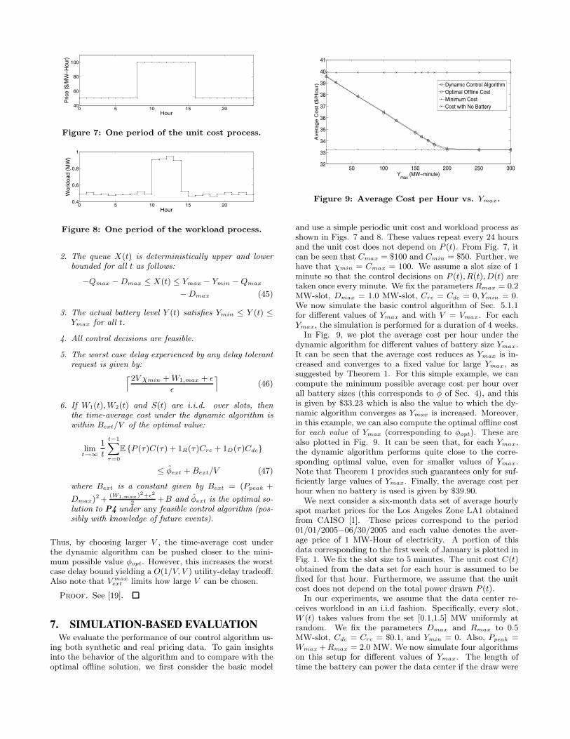
Figure 7: One period of the unit cost process.
0 5 10 15 200.4
0.6
0.8
1
Hour
Wor
kloa
d (M
W)
Figure 8: One period of the workload process.
2. The queue X(t) is deterministically upper and lowerbounded for all t as follows:
−Qmax − Dmax ≤ X(t) ≤ Ymax − Ymin − Qmax
− Dmax (45)
3. The actual battery level Y (t) satisfies Ymin ≤ Y (t) ≤Ymax for all t.
4. All control decisions are feasible.
5. The worst case delay experienced by any delay tolerantrequest is given by:l2V χmin + W1,max + ε
ε
m(46)
6. If W1(t), W2(t) and S(t) are i.i.d. over slots, thenthe time-average cost under the dynamic algorithm iswithin Bext/V of the optimal value:
limt→∞
1
t
t−1Xτ=0
E {P (τ )C(τ ) + 1R(τ )Crc + 1D(τ )Cdc}
≤ φext + Bext/V (47)
where Bext is a constant given by Bext = (Ppeak +
Dmax)2 +(W1,max)2+ε2
2+B and φext is the optimal so-
lution to P4 under any feasible control algorithm (pos-sibly with knowledge of future events).
Thus, by choosing larger V , the time-average cost underthe dynamic algorithm can be pushed closer to the mini-mum possible value φopt. However, this increases the worstcase delay bound yielding a O(1/V, V ) utility-delay tradeoff.Also note that V max
ext limits how large V can be chosen.
Proof. See [19].
7. SIMULATION-BASED EVALUATIONWe evaluate the performance of our control algorithm us-
ing both synthetic and real pricing data. To gain insightsinto the behavior of the algorithm and to compare with theoptimal offline solution, we first consider the basic model
50 100 150 200 250 30032
33
34
35
36
37
38
39
40
41
Ymax
(MW−minute)
Ave
rag
e C
ost
($
/Ho
ur)
Dynamic Control AlgorithmOptimal Offline CostMinimum CostCost with No Battery
Figure 9: Average Cost per Hour vs. Ymax.
and use a simple periodic unit cost and workload process asshown in Figs. 7 and 8. These values repeat every 24 hoursand the unit cost does not depend on P (t). From Fig. 7, itcan be seen that Cmax = $100 and Cmin = $50. Further, wehave that χmin = Cmax = 100. We assume a slot size of 1minute so that the control decisions on P (t), R(t),D(t) aretaken once every minute. We fix the parameters Rmax = 0.2MW-slot, Dmax = 1.0 MW-slot, Crc = Cdc = 0, Ymin = 0.We now simulate the basic control algorithm of Sec. 5.1.1for different values of Ymax and with V = Vmax. For eachYmax, the simulation is performed for a duration of 4 weeks.
In Fig. 9, we plot the average cost per hour under thedynamic algorithm for different values of battery size Ymax.It can be seen that the average cost reduces as Ymax is in-creased and converges to a fixed value for large Ymax, assuggested by Theorem 1. For this simple example, we cancompute the minimum possible average cost per hour overall battery sizes (this corresponds to φ of Sec. 4), and thisis given by $33.23 which is also the value to which the dy-namic algorithm converges as Ymax is increased. Moreover,in this example, we can also compute the optimal offline costfor each value of Ymax (corresponding to φopt). These arealso plotted in Fig. 9. It can be seen that, for each Ymax,the dynamic algorithm performs quite close to the corre-sponding optimal value, even for smaller values of Ymax.Note that Theorem 1 provides such guarantees only for suf-ficiently large values of Ymax. Finally, the average cost perhour when no battery is used is given by $39.90.
We next consider a six-month data set of average hourlyspot market prices for the Los Angeles Zone LA1 obtainedfrom CAISO [1]. These prices correspond to the period01/01/2005−06/30/2005 and each value denotes the aver-age price of 1 MW-Hour of electricity. A portion of thisdata corresponding to the first week of January is plotted inFig. 1. We fix the slot size to 5 minutes. The unit cost C(t)obtained from the data set for each hour is assumed to befixed for that hour. Furthermore, we assume that the unitcost does not depend on the total power drawn P (t).
In our experiments, we assume that the data center re-ceives workload in an i.i.d fashion. Specifically, every slot,W (t) takes values from the set [0.1,1.5] MW uniformly atrandom. We fix the parameters Dmax and Rmax to 0.5MW-slot, Cdc = Crc = $0.1, and Ymin = 0. Also, Ppeak =Wmax + Rmax = 2.0 MW. We now simulate four algorithmson this setup for different values of Ymax. The length oftime the battery can power the data center if the draw were

Ymax 15 30 50Battery, No WP 95% 92% 89%WP, No Battery 96% 92% 88%
WP, Battery 92% 85% 79%
Table 2: Ratio of total cost under schemes (B), (C),(D) to the total cost under (A) for different valuesof Ymax with i.i.d. W (t) over the 6 month period.
Wmax starting from fully charged battery is given by YmaxWmax
slots, each of length 5 minutes. We consider the followingfour schemes: (A) “No battery, No WP,” which meets thedemand in every slot using power from the grid and with-out postponing any workload, (B) “Battery, No WP,” whichemploys the algorithm in the basic model without postpon-ing any workload, (C) “No Battery, WP,”which employs theextended model for WP but without any battery, and (D)“Complete,” the complete algorithm of the extended modelwith both battery and WP. For (C) and (D), we assume thatduring every slot, half of the total workload is delay-tolerant.
We simulate these algorithms to obtain the total cost overthe 6 month period for Ymax ∈ {15, 30, 50} MW-slot. For(B), we use V = Vmax while for (C) and (D), we use V =V max
ext with ε = Wmax/2. Note that an increased batterycapacity does not have any effect on the performance under(C). In order to get a fair comparison with the other schemes,we assume that the worst case delay guarantee that case (C)must provide for the delay tolerant traffic is the same as thatunder (D).
In Table 2, we show the ratio of the total cost underschemes (B), (C), (D) to the total cost under (A) for thesevalues of Ymax over the 6 month period. The total cost overthe 6 month period under (A) was found to be $143, 141.11.It can be seen that (D) combines the benefits of both (B)and (C) and provides the most cost savings over the base-line case. For example, with Ymax = 50 MW-slot, the totalsavings provided by (B), (C), and (D) are $15, 745, $17, 176and $30, 000, respectively.
8. CONCLUSIONS AND FUTURE WORKIn this paper, we studied the problem of opportunistically
using energy storage devices to reduce the time average elec-tricity bill of a data center. Using the technique of Lyapunovoptimization, we designed an online control algorithm thatachieves close to optimal cost as the battery size is increased.
We would like to extend our current framework along sev-eral important directions including: (i) multiple utilities (orcaptive sources such as DG) with different price variationsand availability properties (e.g., certain renewable sourcesof energy are not available at all times), (ii) tariffs wherethe utility bill depends on peak power draw in addition tothe energy consumption, and (iii) devising online algorithmsthat offer solutions whose proximity to the optimal has asmaller dependence on battery capacity than currently. Wealso plan to explore implementation and feasibility relatedconcerns such as: (i) what are appropriate trade-offs be-tween investments in additional battery capacity and costreductions that this offers? (ii) what is the extent of cost re-duction benefits for realistic data center workloads? and (iii)does stored energy make sense as a cost optimization knob inother domains besides data centers? Our technique could beviewed as a design tool which, when parameterized well, can
assist in determining suitable configuration parameters suchas battery size, usage rules-of-thumb, time-scale at whichdecisions should be made, etc. Finally, we believe that ourwork opens up a whole set of interesting issues worth ex-ploring in the area of consumer-end (not just data centers)demand response mechanisms for power cost optimization.
AcknowledgmentsThis work was supported, in part, by the NSF grants CCF-0811670, CNS-0720456, CNS-0615097, CAREER awards CCF-0747525 and CNS-0953541, and a research award from HP.This work was performed while Rahul Urgaonkar was a stu-dent at the University of Southern California.
9. REFERENCES[1] California ISO Open Access Same-time Information System
(OASIS) Hourly Average Energy Prices.http://oasisis.caiso.com.
[2] Lead-acid batteries: Lifetime vs. Depth of discharge.http://www.windsun.com/Batteries/Battery_FAQ.htm.
[3] A. Bar-Noy, Y. Feng, M. P. Johnson, and O. Liu. When toreap and when to sow: Lowering peak usage with realisticbatteries. In Proc. 7th International Conference onExperimental Algorithms, 2008.
[4] A. Bar-Noy, M. P. Johnson, and O. Liu. Peak shaving throughresource buffering. In Proc. WAOA, 2008.
[5] D. P. Bertsekas. Dynamic Programming and Optimal Control,vols. 1 and 2. Athena Scientific, 2007.
[6] J. S. Chase, D. C. Anderson, P. N. Thakar, A. M. Vahdat, andR. P. Doyle. Managing energy and server resources in hostingcenters. SIGOPS Oper. Syst. Rev., 35:103–116, Oct. 2001.
[7] M. Gatzianas, L. Georgiadis, and L. Tassiulas. Control ofwireless networks with rechargeable batteries. IEEE Trans.Wireless. Comm., 9:581–593, Feb. 2010.
[8] L. Georgiadis, M. J. Neely, and L. Tassiulas. Resourceallocation and cross-layer control in wireless networks. Found.and Trends in Networking, 1:1–144, 2006.
[9] S. Gurumurthi, A. Sivasubramaniam, M. Kandemir, andH. Franke. Drpm: Dynamic speed control for powermanagement in server class disks. In Proc. ISCA ’03, 2003.
[10] U. Hoelzle and L. A. Barroso. The Datacenter as a Computer:An Introduction to the Design of Warehouse-Scale Machines.Morgan & Claypool, 2009.
[11] K. Le, R. Bianchini, M. Martonosi, and T. Nguyen. Cost- andenergy-aware load distribution across data centers. In Proc.HOTPOWER, 2009.
[12] A. R. Lebeck, X. Fan, H. Zeng, and C. Ellis. Power aware pageallocation. SIGOPS Oper. Syst. Rev., 34:105–116, Nov. 2000.
[13] D. Linden and T. B. Reddy. Handbook of Batteries. McGrawHill Handbooks, 2002.
[14] M. Marwah, P. Maciel, A. Shah, R. Sharma, T. Christian,V. Almeida, C. Araujo, E. Souza, G. Callou, B. Silva,S. Galdino, and J. Pires. Quantifying the sustainability impactof data center availability. SIGMETRICS Perform. Eval.Rev., 37:64–68, March 2010.
[15] M. J. Neely. Stochastic Network Optimization withApplication to Communication and Queueing Systems.Morgan & Claypool, 2010.
[16] M. J. Neely, A. S. Tehrani, and A. G. Dimakis. Efficientalgorithms for renewable energy allocation to delay tolerantconsumers. In Proc. IEEE SmartGridComm, 2010.
[17] S. Park, W. Jiang, Y. Zhou, and S. Adve. Managingenergy-performance tradeoffs for multithreaded applications onmultiprocessor architectures. In Proc. ACM SIGMETRICS,2007.
[18] A. Qureshi, R. Weber, H. Balakrishnan, J. Guttag, andB. Maggs. Cutting the electric bill for internet-scale systems.In Proc. SIGCOMM, 2009.
[19] R. Urgaonkar, B. Urgaonkar, M. J. Neely, andA. Sivasubramaniam. Optimal power cost management usingstored energy in data centers. arXiv Technical Report:arXiv:1103.3099v2, March 2011.
[20] Q. Zhu, F. David, C. Devaraj, Z. Li, Y. Zhou, and P. Cao.Reducing energy consumption of disk storage usingpower-aware cache management. In Proc. HPCA, 2004.


![[HCI] Week 11. UX Goals and Metrics I](https://static.fdocuments.in/doc/165x107/588a344b1a28abc6168b54cf/hci-week-11-ux-goals-and-metrics-i.jpg)