SHORT TERM LOAD FORECASTING

WITH SPECIAL APPLICATION TO

THE KENYA POWER SYSTEM. &

S h a d ra c h O t i e n o lO r e r o 8 s c . (H O N S ) CELECTR. E S Q )

A t h e s i s s u b m i t t e d in p a r t i a l f u l f i l l m e n t f o r th e d e g r e e o f M aster o f S c ien ce in E l e c t r i c a l E n g i n e e r in g in the

( U n i v e r s i t y o f N a i r o b i .

ipQQ

s

This thesis is my original work and has not been presented for a degree in any other University.

ORERO, S.O.

This thesis has been submitted for examination with my Knowledge as

\

ACKNOWLEDGEMENTS:

The author wishes to acknowledge the many useful

discussions with members of staff of the department of

Electrical Engineering, University of Nairobi,

especially my supervisor, Dr. J.M. Mbuthia who did much

to ensure that this work was completed in good time.

I also wish to thank the Kenya Power and Lighting

Company for giving me all the assistance and the

information that I required for this work.

My thanks also go to my family members, Molly, Curie

and Vicky for their patience and understanding while this

work was going on.

CONTENTS:.FAOJS

✓Abstract ------------------------ -List of Notations and Symbols ------------------ vii

Chapter One : INTRODUCTION --------------------- 1

Chapter Two : MATHEMATICAL THEORY OF THE MODELLING PROCESS

2.0 INTRODUCTION -------------------------- 10

2.1 THE AUTOCORRELATION FUNCTION ------------- 10

2.1.1 Autoregressive (AR) Models ------------- 12

2.1.2 Moving Average (MA) Models ------------- 13

2.2 THE PARTIAL AUTOCORRELATION FUNCTION -- 14

2.3 MIXED MODELS (ARMA) --------------------- 15

2.4 AUTOREGRESSIVE INTEGRATED MOVING AVERAGE

(ARIMA) ALGEBRA -------------------------- 16

2.5 SEASONAL MODELS -------------------------- 18

Chapter Three : MODEL DEVELOPMENT

3.0 INTRODUCTION ---------------------------- 21

3.1 DATA SET DESCRIPTION -------------------- 22

3.1.0 The Kenya Power System Loads ----------- 22

3.1.1 Data Recording ------------------------- 23

3.1.2 Data Analysis ------------------------- 23

3.2 MODEL IDENTIFICATION AND STRUCTURE

DETERMINATION ------------------------- 24

3.3 ESTIMATION OF MODEL PARAMETERS----------- 39

3.3.0 Estimation Theory ----------------------- 39

\

PAGE

3.3.1 EstIllation Method---------------------- 41

3.3.1.1 Hookes and Jeeves Algorithm -------- 43

3.3.2 Parameter Estimates and Diagnostic

Checks -------------------------------- 46

3.3.2.1 Tests of Goodness of fit ---------- 46

3.3.2.2 Fitted Models ---------------------- 47

Chapter Four ; FORECASTING

4.0 INTRODUCTION -------------------------- 56

4.1 THE FORECASTING ALGORITHM ------------- 56

4.2 FORECASTING ERROR MEASUREMENT CRITERIA - 57

4.3 TREATMENT OF ANOMALOUS LOAD PATTERNS-- 58

4.4 LOAD FORECASTING RESULTS -------------- 60

4.5 SOURCES OF ERROR IN FORECASTED LOAD VALUES 70

4.6 AREAS OF POSSIBLE IMPROVEMENT------ 71

Chapter Five : CONCLUSION

5.0 CONCLUSIONS --------------------------- 73

REFERENCES ----------------------------------------- 77

BIBLIOGRAPHY---------------------------------------- 78

APPENDICES ----------------------------------------- 79

CONTENTS:

-VI f-

LIST OF NOTATIONS AND ABBREVIATIONS.,✓

B -

CAPITAL LETTERS.m

Backward shift operator; B Z = Z , m is an integert t-m

D - Degree of seasonal differencing

E - Expectat ion

F -m

Forward shift operator; F Z = Z , m is an integert t + m

L - Load forecast lead time in hours

N - Number of original load series observations

P - Number of seasonal autoregressive parameters

Q - Number of moving average prarmetersW - Differenced load series observations

Z -

z -t

Load demand in megawatts

Load forecast at time origin t

SMALL LETTERS

a - t

d -

Normally distributed residual

Degree of regular differencing

k - Lag of autocorrelation and partial autocorrelation

functions

1 - Load forecast lead time in hours

m - Integer

n Number of observations in the differenced load

series observations

P ~ Number of regular autoregressive parameters

q - Number of regular moving average parameters

\

- v i i i -

b - Seasonal period in hours

t - tine in hours

GREEK LETTERS,V - Differencing operator, V Z =Z -Z , m is an integer

m t t t-m

0 , 1=1,..,p are autoregressive parameters in the model i

9 , 1=1,..,q are moving average parameters in the model1

o' - Standard deviation a

2X - Chi squared statistic

ABBREVIATIONS.

ACF -Autocorrelation function

ACCFS -Autocorrelation function coefficient

AR -Autoregressive

ARMA - Autoregressive moving average

ARIMA - Autoregressive Integrated Moving AverageG.P.O -General post office

IBM - International business machinesMA - Moving average

ND - Degree of regular diffe-encing

NM - Number of regular moving average parametersNO - Number

NSR - Degree of seasonal autoregressive parameters K P& T - Kenya posts and telecommunications

PACF - Partial autocorrelation-function

PACCFS - Partial autocorrelation function coefficients

PAS - Power apparatus and systems

SC’ADA- System control and data acquisition.

SE - Standard error

SPSS - Statistical Package for social scientists

V.H.F - Very high frequency

Vol. Volume

- 1 -

CUAfTEB -1

INTRODUCTION

Power system operation and control requires, among

other things, an accurate knowledge of the total system

load demand. The main objective of effective power

control is to regulate the generated power so as to

follow the fluctuating load and then to maintain the

system frequency within an allowable range.

In the past resources were abundant, fuel supplies

were cheap and load forecasting did not receive the

attention it deserved. The daily economic operation

activities such as load flow studies, generation plant

load scheduling, unit commitment, system security and

contingency analysis and short term maintenance planning

all require short terra load forecasts for a period

ranging from about 1 hour to 24 hours.

In a mixed hydrothermal system like the Kenyan

case under study, the preparation of thermal and geother­

mal plants require much time before bringing them on

line and a load forecast several hours ahead is required

before committing such units. Kenya at the moment is

interconnected with the Ugandan power system and plans

are underway to interconnect with neighbouring Tanzania.

Short term load forecasts will be useful in the energy

trade with these utilities.

The subject of short term load forecasting has

- 2 -

received widespread attention" for more than a decade

now. This is due to the ever pressing need to use the

available scarce resources as economically as possible

and also due to the availability of cheap and powerful

computers for the analysis of power system load charac­

teristics .The review paper by Abu-El-Magd and N.K.Sihna [11

gives an overview of the work that has been done in the

area of 3hort term load forecasting. All these proce­

dures require modeling of the power system load demand

characteristics and thereafter evaluating the model

parameters to be used in the forecast algorithm for

producing the desired load prediction.

The forecasting techniques can broadly be classi­

fied into two classes;

1) Methods involving past load data only;

2) Methods involving both past load data and weather

variables;Amongst the most widely used forecasting

techniques are;

1. Regression based algorithms, where the relationship

between the residuals of the load and the weather varia­

bles is modeled using the mathematical techniques of

linear regression analysis [2].Multiple regression models are based on

explanatory variables, and for a given time series, the

-3 -

explanation variables are selected on the basis of the

correlation analysis of the load series. For example a

multiple regression model can be written as;

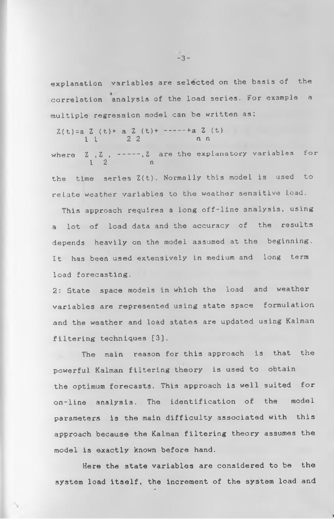
Z(t)=a Z (t)+ a Z (t)+ ---- +a Z (t)11 2 2 n n

where Z ,Z . -----,Z are the explanatory variables for1 2 n

the time series Z(t). Normally this model is used to

relate weather variables to the weather sensitive load.

This approach requires a long off-line analysis, using

a lot of load data and the accuracy of the results

depends heavily on the model assumed at the beginning.

It has been used extensively in medium and long term

load forecasting.2: State space models in which the load and weather

variables are represented using state space formulation

and the weather and load states are updated using Kalman

filtering techniques [3].The main reason for this approach is that the

powerful Kalman filtering theory is used to obtain

the optimum forecasts. This approach is well suited for

on-line analysis. The identification of the model

parameters is the main difficulty associated with this

approach because the Kalman filtering theory assumes the

model is exactly known before hand.

Here the state variables are considered to be the

system load itself, the increment of the system load and

-4-

the short terra and long term ldad patterns, different

models being developed for different time frames.

For example, in daily load forecasting some periodical

load pattern is contained and the effects of the weather

conditions on the system load cannot be neglected. Thus

the model can be written as;

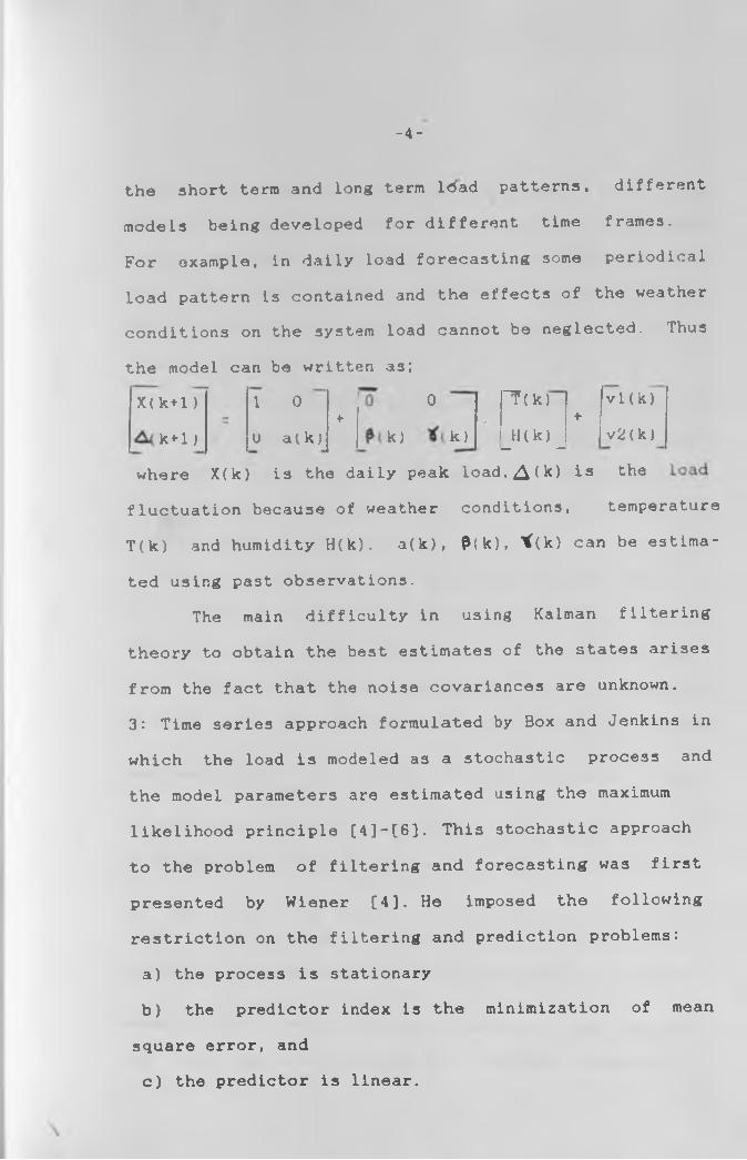
X( k+1) 1 0>

0 “T(k)+

v 1 (k)

k*l) U a( k) k) k) H(k) v2(k)_ —

where X(k) is the daily peak load.^(k) is the

fluctuation because of weather conditions, temperature

T O O and humidity H(k). a(k), P(k), *(k) can be estima­

ted using past observations.The main difficulty in using Kalman filtering

theory to obtain the best estimates of the states arises

from the fact that the noise covariances are unknown.

3: Time series approach formulated by Box and Jenkins in

which the load is modeled as a stochastic process and

the model parameters are estimated using the maximum

likelihood principle [4]-[6]. This stochastic approach

to the problem of filtering and forecasting was first

presented by Wiener [4]. He imposed the following

restriction on the filtering and prediction problems:

a) the process is stationary

b) the predictor index is the minimization of mean

square error, and

c) the predictor is linear.

-5 -

With the above assumption^ one only needs the

autocorrelation function of the process and the noise

input, and the cross-correlation function of the two.

This idea was extended by Box and Jenkins [4] for

handling a class of non-stationary processes by a finite

linear transformation.

The determination of the model order is done by

examining the pattern of the sample autocorrelation

function, as well as the partial autocorrelation

functions [4], Such correlation plots is for identifying

possible underlying behaviour.

4. Methods based on spectral decomposition [7]-[8].These methods divides the load demand into various

components. For example, Farmer et al [8], divides the

load into 3 components; a long term trend, a component

varying with the day of the week, and a random

thcomponent. If Z (t) denotes the load in the W week

wdth

of the year, on the d day of that week, and the time

of the day (t), then Z (t) is expressed in the form;wd

Z (t)= A (t ) + B (t) + X (t) wd w d • wd

where A (t) represents a trend terra which is updated w

weekly, B (t) denotes a term dependent on the day of d

the week, and X (t) denotes the residual component.wd

-6-

The terms A (t) and B (t) are fdund by minimising the w d

mean square error of the random component average over

several weeks of past data. This method requires a lot

of past load data for analysis and this means a lot of

computer memory is required for effective analysis,

which is its main drawback.

5: Christiaanse, [9], for instance used the general method

exponential smoothing where the weekly variations in hou­

rly load are described as a cyclic function of time with

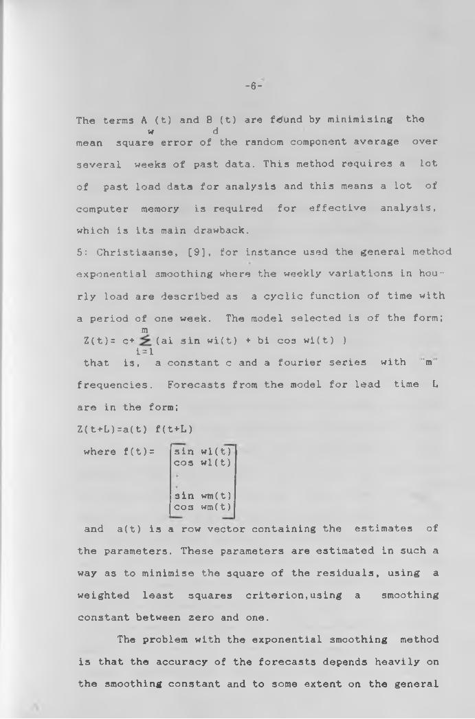
a period of one week. The model selected is of the form; m

Z(t)= c+ (ai sin wi(t) + bi cos wi(t) ) i = 1

that is, a constant c and a fourier series with m

frequencies. Forecasts from the model for lead time L

are in the form;

Z(t+L)=a(t) f(t+L)

where f(t)= sin wl(t) cos wl(t)

3in wm(t) cos wm(t)

and a(t) is a row vector containing the estimates of

the parameters. These parameters are estimated in such a

way as to minimise the square of the residuals, using a

weighted least squares criterion,using a smoothing

constant between zero and one.

The problem with the exponential smoothing method

is that the accuracy of the forecasts depends heavily on

the smoothing constant and to some extent on the general

-7 -

form of the model chosen beforehand.Observations from a naturally occurring phenomena

such as load demand which depends on a number of inter­

related variables such as economic factors, social beha­

viour of consumers, effects of weather and other unquan-

tifiable factors, posses an inherent probabilistic struc­

ture. Deterministic models cannot be obtained for such

systems and stochastic models have been employed widely

to model such series.In this study, the time series analysis system

identification approach to stochastic model building has

been chosen to analyse the load using past data only.

The exclusion of weather variables is due to • the fact

that Kenya is basically a tropical country and the

amount of installed equipment that is sensitive to wea­

ther ( such as space heaters, air conditioners etc. ) is

minimal. The other factor is due to the non-uniformity

of weather conditions in various parts of the country

which would make it difficult to include them in a study

of this magnitude. Inclusion of such variables would

also involve a prediction of weather parameters as well

and this could possibly lead to more errors because of

the double forecasting process.

The main advantage of the time series approach to

short term load forecasting are it’s ease of underst­

anding, implementation and the accuracy of it’s results.

-8 -

There are many approaches to time series analysis

including the better known regression analysis. The

general mixed autoregressive integrated moving average

(ARIMA) modeling approach pioneered by Box, G.E and

Jenkins [4] for any stochastic process has many

advantages over the alternative modeling approaches.

The beauty of the ARIMA approach is that Box and

Jenkins have laid a firm and rigorous mathematical basis

for its analysis. In the case of seasonality or period­

icity in the data for instance, the alternative appro­

aches often require a seasonal adjustment of the time

series prior to analysis. The ARIMA approach in contrast

models the dependencies which define seasonality. Ano­

ther case is in the treatment of growth and trend eff­

ects in the series; while other techniques require sepa­

rate treatment of such terms, the ARIMA approach takes

care of such adjustments in the modeling process by a

linear transformation of the original series into a

stationary time series. These advantages are brought out

clearly in a study by Plosser [10].

This particular study is unique in the sense that

every power system is different from each other. Every

system has its' own load demand characteristics and

no load forecasting programme can be universally appl-

ied. A load forecasting programme can be developed for a

system only after its load demand characteristics are

I -9-

modeled and understood. ✓

In Kenya, at the moment there is no proper load

forecasting procedure. Much depends on the experience of

the System controller on duty who uses his own judgment

and past experience. While such forecasts are sometimes

accurate, most times they lead to gross errors and hence

uneconomic operation of the system.

It can be seen that there is an urgent need for a

3hort term load forecasting algorithm for the Kenya

power utility. A prediction scheme which provides accu­

rate estimates of the load demand a few hours a head

satisfies the requirements of the control system for

which this study is based.

This study sets out to develop a load forecasting

programme for the Kenya power system based on a sound

mathematical and scientific load forecasting technique.

It makes use of the available and affordable personal

computer to develop the programme. The quantity to

be forecast is the total average hourly load demand in

megawatts. New forecasts are to be computed each hour,

immediately following the reading of the integrated load

demand of the previous hour.

-10-

MATHEMATICAL THEORY 01 THE MODELING PROCESS

2.0 INTRODUCTION

Time series analysis is essentially concerned

with evaluating the properties of the probability model

which generated the observed time series. In this

analysis the evolving load demand is assumed to be a

stochastic process which can be described by some of the

moments of the generating process such as the mean, var­

iance and autocovariance functions. At its basis, a

time series process consists of a random shock or white

noise inputs and a realization or observation

outputs, which in this case are the hourLy megawatt totaL

system load demand.

2.1 THE AUTOCORRELATION FUNCTION (ACF).

A stationary stochastic process is fully

determined by its mean, variance and autocorrelation

function. If two processes have the same three

variables, then they are the same process.

Since each distinct process has a unique

autocorrelation function, the autocorrelation function

can be estimated from a realized time series and that

information used to determine the process structure

which generated the realization.

For a Z time series process, the autocorrelation t

UHAfJEB 2

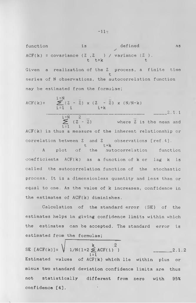
- 1 1 T

function la defined as*

ACF(k) = covariance (Z ,Z ) / variance (Z ).t t + k t

Given a realization of the Z procesa, a finite timet

series of N observations, the autocorrelation function

may be estimated from the formulae;

i = NACF (k ) = ^.(Z - Z) x (Z - Z) x (N/N-k)

i=l i i+k________________________________ _____2.1.1i=N 2.2E (Z - Z) where Z is the mean andi = l i

ACF(k) is thus a measure of the inherent relationship or

correlation between Z and Z observations [ref.4].t t + k

A plot of the autocorrelation function

coefficients ACF(k) as a function of k or lag k is

called the autocorrelation function of the stochastic

process. It is a dimensionless quantity and less than or

equal to one. As the value of k increases, confidence in

the estimates of ACF(k) diminishes.

Calculation of the standard error (SE) of the

estimates helps in giving confidence limits within which

the estimates can be accepted. The standard error is

estimated from the formulae;

\ *SE [ACF(k)]= V l/N(l+2 £.ACF(i) ) _______2.1.2i = l

Estimated values of ACF(k) which lie within plus or

minus two standard deviation confidence limits are thus

not statistically different from zero with 95% confidence [4].

■ v

-12-

2.1.1 AUTOREGRESSIVE (AR) MUDKULs

thA p order autoregressive process is written as;

Z-j^Z *■..... + fa Z <- a ______ 2 . L . 1. Lt 1 t-1 2 t-2. p t-p t

In this model, the current value of the process is

expressed as a finite, linear, aggregate of previous

values of the process and a shock a .t

Une of the most common autoregressive processes is

that of order one, written as Z -^Z > a __ 2. 1.1.2t 1 t-t t

The ACF of this process is expected to decay

exponentially from lag to lag.

Some operators used in simplifying the analysis ot

the models are;

1) The backward shift operator, B which is defined asm

BZ =Z , thus B Z -Z t t-1 t t -m

2) The inverse operation is performed by a forward shift -l m

operator F=B given by FZ -1 , hence F Z =Zt t+1 t t*-m

3) The difference operator, V which can be written as

V Z = Z - Z t t t-1

A general autoregressive operator of order p can, 2 p

be defined by P( B ) = 1 - fi B- <p B -.... - <f> B ____ 2.1.1.31 2 p

hence equation 2.1.1.1 of the general AR model can be

economically written as; .

0(B)Z = t t

2.1.1.4a

-13-

Thus an AR process can be considered as the output Zt

trom a linear filter with a transfer function A B) when

the input is white noise, a .t

2.1.2 MOVING AVERAGE LtfAl MODELSIn practice, the time series analysis begins with

an autocorrelation function estimated from the original

or raw time series, L . If the AGF indicates that thet

process is non-stationary,then the series must be

differenced. The second stage of the analysis is an

identification of a model for the stationary series

based on the serial correlation patterns shown in the

autocorrelation function.th

One class of serial dependency is the q order

moving average process. Here Z is linearly dependent ont

a finite number of q previous a ’s. Thus

Z =a -0 a -0 a -....-0 a ___ 2.1.2.1t t 1 t-1 2 t-2 q t-q

A general moving average operator of order q can be

defined by2 q

0(B)=l-0 B-0 B -...... -0 B ____2.1.2.21 2 q

hence the moving average model can be written as

Z = 0(B) a ____2.1.2.3t tAn MA process of order one is expected to have a non­

zero value of ACF(l) while all the successive lags of

the ACF(k) are expected to be zero.th

In general, a q order MA process is expected to

-14-

have non-zero values of ACF(l).... ACF(q). The values of

ACF(q+l) and beyond are all expected to be zero, thus an

MA process model identification is based on a count of

the number of non-zero spikes in the first q lags of the

ACF.

2.2 HIE PARTIAL AUTOCORRELATION FUKCUflM LEAC£1This is a useful statistic for model

identification. It is a complementary tool to the

autocorrelation function in the identification of time

series models.

The lag k partial autocorrelation

function, PACF(k) is a measure of the correlation between

time series observations k units apart after correlation

between intermediate lags have been removed or

’partialled’ out. Unlike the autocorrelation

function, the partial autocorrelation function cannot be

estimated from a simple straight forward formulae.

It is usually estimated from the autocorrelation

function since it is a function of the expected

autocorrelation function [4].

The below formulae is used to estimate the

partial autocorrelation function. The PACF at lag k is

denoted byj2f(kk) and if the ACF at lag k is denoted by

r then; k

\

-15-

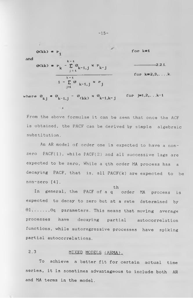
0Ock) - r

andk - i

<xuo ■ - k - r V . .J * V jJ= i

1 - V 0 k-i.j* -j

wher. 0kJ - 0k., j - 0<kk> « V l J r j

for k-1

-------------- 2.2 .1.

for k.a2,3,. . . .k

for J-1,2,. . .k-1

From the above formulae it can be seen that once the ACF

is obtained, the PACF can be derived by simpLe algebraic substitution.

An AR model of order one is expected to have a non­

zero PACF(l), while PACF(2) and all successive lags are

expected to be zero, While a qth order MA process has a

decaying PACF, that is, all PACF(k) are expected to be non-zero [4].

thIn general, the PACF of a q order MA process is

expected to decay to zero but at a rate determined by

..... >©d parameters. This means that moving average

processes have decaying partial autocorrelation

functions, while autoregressive processes have spiking partial autocorrelations.

2.3 MIXED MODELS (ARMA).

To achieve a better fit for certain actual time

series, it is sometimes advantageous to include both AR and MA terms in the model.

-16-

The relationships in the autoregressive and moving

average processes so far discussed place some limits on

mixed models. Such relationships sometimes lead to

parameter redundancies, because at times comp lex models

are equivalent to simpler models with fewer parameters.

Both the ACF and PACF of a mixed process are expected

to decay. A general mixed ARMA model can be written as;

Z -<f>l + .... + 0 Z * a -8 a a __2.3.1. t 1 t-l P t-p t L t-1 q t-qThe general equation for a mixed model can then take the

the form (B)2 =8(B) a ----------2.3.2t t

in practice it is frequently true that adequate

representation of actually occurring stationary series

or one that has been made stationary by transformation

can be obtained with AR, MA or mixed modeLs in which

the order is not greater than two.

2.4 AUTOREGRESSIVE INTEGRATED MOVING AVERAGE ( AR1MA J ALGEBKA

An observed time series,in our case the hourly

load demand denoted as Z ,Z .......Z ,Z .can be1 2 t-l t

described as a realization of a stochastic process.

At the heart of the generating process is a sequence

of random shocks, a , which conveniently summarize thet

multitude of factors producing the variation in the load

demand. For computational simplicity it is assumed that

the random shocks are normally and independently distributed.

Many actual series exhibit nonstationary behaviour and d

not vary about a fixed mean. In particular, although th

\

-17 -

gene ral level about which fluctuations are occurring may be

different, the behaviour of the series, when differences in

level are allowed for, may be similar. Thus a general model

which can represent non-stationary behaviour is of the form

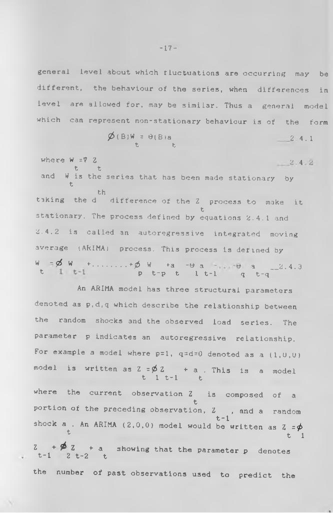
^ (B)W = d(Bla 2 4.1t t

where W =V Z At t

and W is the series that has been made stationary by t

thtaking the d difference of the Z process to make it

tstationary. The process defined by equations 2.4.1 and

2.4.2 is called an autoregressive integrated moving

average (AklMAj process. This process is defined by

w ~ & w *....... +0 W +a - H a a _2.4.3t P t-p t 1 t-l q t-q

An ARIMA model has three structural parameters

denoted as p,d,q which describe the relationship between

the random shocks and the observed load series. The

parameter p indicates an autoregressive relationship.

For example a model where p=l, q=d=0 denoted as a (1,U,U)

model is written as Z = 0 Z + a . This is a modelt 1 t-l t

where the current observation Z is composed of at

portion of the preceding observation, Z , and a random . , t-lshock a . An ARIMA (2,0,0) model would be written as Z =56

1 t 11 + * Z * a showing that the parameter p denotest-l 2 t-2 t

the number of past observations used to predict the

-18-

current observation. s

The structural parameter q denotes the number of

moving average structures in the model. An ARIMA (0,0,1)

model would thus be written as Z = a - 0 a and at t 1 t-1

(0,0,2) model would be written as Z = a - 0 a - 0 at t 1 t-1 l t-2

An ARIMA (0,0,q) model is one where the current

observation, Z is composed of a current random shock a t t

and a portion of the q-1 preceding random shocks, at-1

through at-q

Finally the structural parameter d indicates that

the time series observations have been differenced.

Differencing amounts to subtracting the first

observation from the second, second from third and so on.

This i3 usually performed on a non-stationary time

series to make it a stationary process. An ARIMA

(0,1,0) model would be written as Z -Z = a . Thist t-1 t

means that the current observation, Z is equal to thet

preceding observation, Z plus the current shock at-1 t

Model identification refers to the empirical proce­

dures by which the best set of parameters P.d.q are

selected for a given load series.

2.5 MODELS.

Seasonality is defined as any periodic or cyclic

behaviour in the time series. The ARIMA approach of

-19r

analysis models dependencies which define seasonality.

There also exist seasonal ARINA structures denoted by

P.D.Q.P denotes the number of seasonal autoregressive

parameters, Q the number of seasonal moving average

parameters and D the degree of seasonal differencing.

If a series exhibits seasonal non-stationarity,to

make it stationary it must be differenced with respect to the seasonal period. Seasonal autoregression is where

the current observation depends upon the corresponding

observation of the series for the preceding period or

season. Seasonal moving average is when the current

observation depends upon the random shock of the

preceding period.

Similar rules of regular ARIMA (p.d.q) models also

apply to seasonal time series analysis. Identification

of a seasonal ARIMA structure proceeds from an

examination of the ACF and PACF of the raw data. The

only difference between seasonal and regular models i3that for the seasonal processes, patterns of spiking and

decay in the autocorrelations and partial

autocorrelations appear at the seasonal lags.

Seasonal non-stationarity is indicated by an ACF

that dies out slowly from seasonal lag to seasonal lag.

Seasonal autoregression is indicated by an ACF that dies

out exponentially from seasonal lag to seasonal lag

while the ACF of a seasonal moving process spikes at the

-20 -

seasonal lags.Most time series with seasonal ARIMA behaviour

also exhibit regular behaviour as well. A powerful model

can be realized by incorporating regular and seasonal

structures multiplicatively, an example of such a model

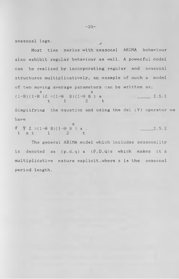
of two moving average parameters can be written as; s s

(1-B)(1-B )Z = (1-0 B ) ( l - e B ) a _____2.5.1t 1 2 t

Simplifying the equation and using the del (V) operator we

haves

7 7 Z =(1-0 B)(1-0 B ) a . _____2.5.21 s t 1 2 t

The general ARIMA model which includes seasonality

is denoted as (p.d.q) x (P,D,Q)s which makes it s

multiplicative nature explicit,where s is the seasonal

period length.

- 2 1 -

CHAPTER 3

MOQKL DEVELOPMENT

3.0 INTRODUCTIQtL

Having developed the theory behind ARIMA models,

the problem of building a model for the load time

series i3 now addressed.The model building strategy is based on three

procedures of identification, estimation and diagnosis.

The main aim is to construct a model which is

statistically adequate 33 well as parsimonious (having

the minimum number of parameters).

The model building process is summarised by the

block diagram below:

-22-

(z}<—

3.1 DATA SET DESCRIPTION.

3.1.0 XHE KENYA POWER SYSTEM EOAP^.The Kenya power utility is a small power

system with a total peak load demand of 460 megawatts to

date. The total energy consumption per day is about

8,500 megawatt hours. The domestic consumers constitute

about 35* of this demand while the remaining 6b% is

mainly industrial and small scale commercial consumers.

-2.3-

3.1.1 DATA

There is a manual recording of megawatt hour

readings from printographs located at each power genera­

ting station. Control attendants at these stations take

Load readings of the power generated from each machine

every half an hour, sum up the total readings for the

station, and then relays the information to another con­

trol assistant at the national control centre through

K.P&T public telephone, power line carrier or V.H.F radio

These readings are then logged into a master log

sheet at the control centre as they arrive and are

thereafter used by the system controllers for system

operation. At the end of a 24 hour period the log sheet

is kept filed. It can thus be seen that data collection

and retrieval is a tedious and difficult process.

3.1.2 DATA ANALYSIS

Some readings of the half-hourly load readings

for 1987 and part of 1988 was collected at the Kenya

power and lighting utility national control centre. The

half hourly load readings are averaged to obtain the

hourly readings which are then entered into a load data

file for computer analysis.

Six weeks of data were used for model development.

Six weeks of data were analysed for four different

periods in the year for a comparison to see whether the

load model structure and parameters change significantly

-24-

within the year. *

Data for periods as long as twelve weeks were analysed

for some of the periods to observe the behaviour of the

model structure and parameters as the size of the data base increased.

3.2 MODEL IDENTIFICATION AND STRUCTURE DETERMINATION.

The key to model identification is the human pat­

tern recognition of the autocorrelation and partial

autocorrelation functions of the various forms of the

load time series observations.

The estimated ACF and PACF will indicate whether the

series is stationary or not, the existence of any seaso­

nal patterns and whether the series is a moving ave­

rage, autoregressive, mixed ARMA or just white noise

process. The general ARIMA model can be denoted as;

(P.d.q) x (P,D,Q)s .

Where p denotes the number of regular autoregressive

parameters, d the degree of regular differencing, q the

number of regular moving average parameters, P the number

of seasonal autoregressive parameters, D the degree of

seasonal differencing, Q the number of seasonal moving

average parameters and s the seasonal period. The values

of the parameters p,d,q as well as P,D,Q and s can also be obtained from these plots.

The analysis begins by looking at the plots of

these functions which are obtained from the programs

\

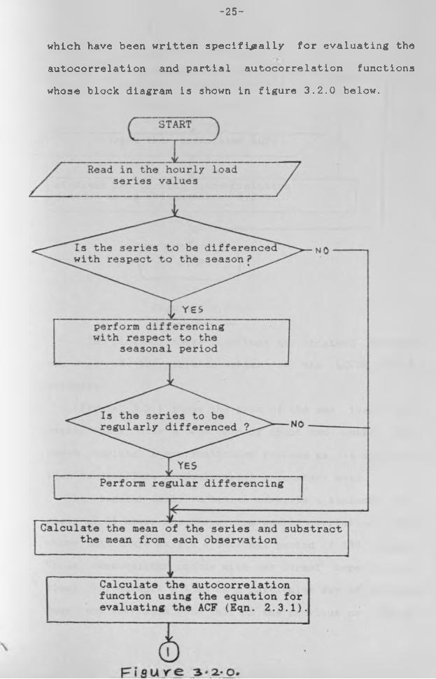
-25 -

which have been written specifically for evaluating the

autocorrelation and partial autocorrelation functions

whose block diagram is shown in figure 3.2.0 below.

-26 -

Figure 3.2.0.

The plots of these functions are obtained through

the use of the graphics option of the LOTUS 1-2-3 software.

Figure 3.2.1 shows the plot of the raw load time

series data over a time span of about two weeks. The

curve depicts a non-stationary process as it does not

seem to oscillate randomly about a constant mean.

The regular daily variation suggests a seasonal pe­

riod of 24 hours and the strong weekly variation also

shows that there exists a seasonal period of 168 hours.

These observations concur with our normal expectations

since, for example a load on a particular day of the week

does not vary much from that of the previous or coming

\

27\

LOAD IN MEGAWATTS

Figure 3.2.1

TYPICAL HOURLY LOAD PATTERNS

- 2 a .-

week on the same day, likewise the load at a particulars

hour of the day will not be much different from that

of the same hour on the the next or previous day, for

similar days of the week, for example, a monday and a

tuesday load at 18.00 hours are expected to be quite

similar.Figure 3.2.2 shows the plot of the autocorrelation

function of the raw data, the original load series before

any data transformation. The ACF starts with high posi­

tive values and dies out slowly from seasonal lag to

seasonal lag,the significant seasonal lags being 24 and

168 hours. This pattern suggests non-stationarity in the

series which means the series should be regularly diffe­

renced, (d=l).

Figure 3.2.3 shows the ACF estimated from the regu­

larly differenced series, (d=l). Seasonal non-stationarity

is still persistent as evidenced by the slow decay of

the ACF from lag to lag. The key seasonal lags still

being 24 and 168 hours.

Figure 3.2.4.1 shows the ACF of the series diffe­

renced only with respect to a period of 24 hours, s=24

and D=l.

There are significant spikes at lags 168 and 336 hours

as well as a slow decay in the ACF which indicates that

there should be regular as well as seasonal differen­

cing.

\

2 .3

ACCFS

\ Figure 3.2.2

ACTS GRAPH(N

0=

2I8

4 D

=0

d=

0 )

AC

CF

S

ACFS GRAPH( N0=2184 D=0 4 = I )1 ------------------------------------------------- -

0.9 -

0.8 -

0.7 ~

0.6 -

0.5 -

0 24 48 72 9 6 120 144 168 192 216 240 264 288 312 336 360 334

Fig

ure

3

.2.3

.

- 3 1 -

AJCQFS

1o 1O 1o o o o o O O O o oki - O - Kj o« Oi cn -J i'B <0

_—1- —1-------- 1— i ■ . 1.._J___1— 1 ■ 1 1

Figure 3 .2 .Jl.l

ACFS GRAPH(N

0=

2I8

4 D

=l

MS =

24

d=

- 3 2 *

Figure 3.2.4.2(a) shows the ACF of the series diff­

erenced regularly (d=l) as well as seasonally (D=l), with

a period of 24 hours. Significant spikes at

ACF(l), ACF(24), ACF(25) indicate the presence of a regu­

lar moving average (q = l) and a seasonal moving average

process (Q=l). There also appears to be a significant

3pike at lag 163 hours and 336 hours, the value at 336

being less than that at 168 hours. These additional

spikes indicate the possibility of a seasonal autoregre­

ssive parameter of order one, (P=l and s=168). The

remaining lags can be said to be nearly zero with 95%

confidence and the series does not therefore require any

further differencing.

Figure 3.2.4.2(b) shows the partial autocorrela­

tion function from the same data set that generated

figure 3.2.4.2(a). There are significant spikes at seaso­

nal lags which are multiples of 24 hours which progres­

sively decrease exponentially from lag 24, confirming

the existence of a seasonal moving average operator of

order one. The PACF pattern confirms the assertion that

the process is a seasonal moving average of order one

and a tentative model for further consideration can be

identified at this stage. This model is of the form;24

V 7 Z = (1-0 B)(l-9 B ) a ____3.2.124 t 1 2 t

Figure 3.2.5.1 shows the ACF of the series differe­

nced only with respect to a period of 168 hours, (D=l and

\

ACCFS

1o

1o

1o

»o 1o o o o o o o o O <0

oi o» fo — o — h <ji +* Cn b> Al (n <j’j —

4 -_1___1_--1- 1 J -J___L.-J___L_ _J___ 1___

■ i t

Figure 3.2 .^ .2 (a )

ACFS GRAPH(N

0=10O

B N

S=24 D

= I

d=

PA

OG

FS

PACCFS-GRAPH(N 0 = 1008 N 5 =2 4 N D = 1 )

0 24

Figure 3

.2A2

. (b)

■ ....I.i..in..lmnm.iiniimiilinmiimumittlllllllllliuillllllll

tmiliuillliulll

iuum

unuillinlu«iuuuil

3>£-

P i p - u r e 3 . 2 . 5 . 3

ACFS GRAPH(N0=2184 D= 1 rc=168 d =

-36-

s = 168 ). There is only a significant spike at lag 168

hours, otherwise the ACF also dies out slowly to zero

indicating the necessity of regular differencing as

well.

The load series is differenced regularly as well

as seasonally with a period of one week, (d=l,D=l and

s= 168 ).

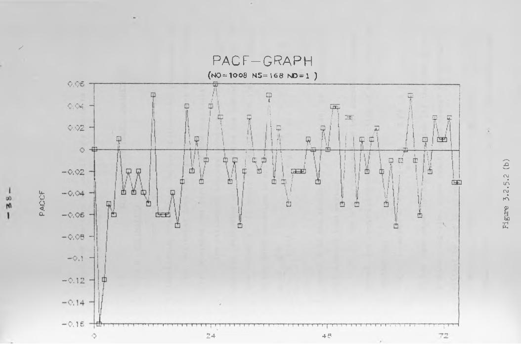
Figure 3.2.5.2(a) shows the ACF of this series.

Significant spikes appear only at lags l and 168

suggesting the presence of a regular moving average

operator of order one (q-1) as well as a seasonal moving

average parameter of order one (Q=l and s=168).

Figure 3.2.5.2(b) shows the PACF plot corresponding

to figure 3.2.5.2(a). This figure confirms the deductions

made from the ACF plots. A seasonal MA process of order

one is indicated by the PACF pattern. The exponential

decay of the PACF from lag one indicates the presence of

a regular moving average process of order one. The rest

of the lags of the PACF and the ACF plots can be

considered to be zero with 95% confidence. Another

possible tentative model is thus entertained of the

below structure;

168V V Z = (1-9 B) (1-0 B ) a _____3.2.2

168 t 1 2 t

The parameters of the two identified models then

have to be estimated from the data and diagnostic checks

\

rrflI

ACFS GRAPH(NO= 1008 NS=16S 0=1 d = l )

Figure 3

.2.5.2 (a)

PACCF

/

PACF—GRAPH(NO=:1008 N5= \ 6 8 NJD - 1 )

24 4?

Figure 3

.2.5.2 (b)

- 3 9 -

performed on them to see if th^y could be adequate for

load forecasting.

3-3 ESTIMATION QE MODEL EARANETEJiS^

3.3.0 ESTIMATION THEORY■

Once the model structure has been tentatively

identified, the actual values of the model parameters are

then estimated from the data by searching those values

that minimise the variance of the residuals (a ).t

The estimation process involves looking for least

squares estimates which minimise the sum of squares of

the noises a . In order to calculate the a ’s, the general t t

mixed ARIMA equation is written as:

a =W - $6 W -....... -<£ W ♦ 0 a + ........ f0 at t 1 t-1 p t-p 1 t-1 q t-q

______3.0.1

where W is the stationary load series, or appropriately t

differenced load series.

Since the a’s are assumed to be normally distri- t

buted, the probability density function of the a ’s can bet

written as;-n n 2 2

P(al.... .anl^a'a exp{ -( ^ a / 2 ^a ) } _____3.0.2t = l t

It has been shown by Box and Jenkins [4] that the uncon­

ditional log-likelihood function is needed for parameter

estimation and is given by;2

L(£,0,da )= ) - n Lnfl'a - S(^>,6)/2tfa_____3.0.3

where f(^,9) is a function of <f> and 9. The unconditional

\

-40

sura of squares function is given by;n 2 X

S<^.6 )= [a J _____ 3.0.4t = l t

where [a ]-E[a ;^,9.w| denotes the expectation of at t *■ t

conditional on <£,0 and w.NormaLly r 1 <£ , u j 13 or importance only when the

number of terms in the series (n) is small. When n is

large S(0,9) dominates the log-1ikelihood function and

it follows that the parameter estimates which minimise

the sum of squares will be a close approximation to the

maximum likelihood estimates.

In order to calculate the unconditional sum of

squares it is necessary to estimate the values of

W ,W ......... W of the series which occurred beforeo l -Q

the first observation of the series was made.

This enables the starting off of the difference

equation 3.0.1 .

To facilitate this backward estimation ,the forward

form of the general model equation is introduced where-1

all B ’s are replaced by F’s, (F = B ).

0 (F) = 9(F) e ort

W - W -..... - W = e -0 e -.....9 q e ____3.0.5t t+1 t+p t t+1 t+q

where {e } is a sequence of independently distributed t

normal random variables. This process is a stationary

-41-

representation where W ig expressed in terms oi W's andt

e ’s and this model and the backward model of equation

3.0.1 have identical probability structures.

With the forward shift operator.it is possible to

use equation 3.0.5 to estimate W ’s which occurred prior

to the first observation. To calculate the unconditional

Siam of squares S<j2f. 0 ) for any given set of parameters &

and 9. equation 3.0.5 is fir3t used to estimate the W ’sprior to the start of the series.then these initial

values are used with equation 3.0.1 to estimate the [a

‘sj and finally the [a ’s] are summed to obtain S(^, 9i.t

3.3.1 ESTIMATION MEIHQP,Model estimation is an optimisation process

that requires a suitable software package. The general

ARIMA model is non-linear in it’s parameters, so standard

software regression packages such as SPSS cannot be

used. There are several mathematical optimization methods

which can be used for non-linear least squares estimation.

The method to be used in any optimization problem

will depend on the nature of the problem. If the problem

is formulated mathematically in an analytical form. the0

method chosen will depend on whether;

1) it is a static or dynamic optimization process

2) the performance function is constrained or not

3) the objective function is linear or non-linear

V

-42-

4) the function is single variable or multi-variable.

In this work static optimization will be used. In

principle, static systems are those whose parameters do

not change with time, however,systems whose parameters

vary slightly within a reasonable range of time will

also be considered static. It is also a non-linear

formulated problem, with more than one parameter to be

estimated.

The methods which have been successfully usedinclude the Marquardt algorithm, conjugate gradient

method of Fletcher and Reeves, Hookes and Jeeves

optimization method, Descent method of Fletcher and

PoweLl among others [1J. All these methods and their

algorithms are fully discussed in any standard

optimization mathematics text [11].In this work, the method of Hookes and Jeeves [12]

has been chosen because it is easier to understand and

program and its computer memory requirements are less, a

factor that is of considerable importance since this

work is being developed for use on a personal computer.

It also meets the conditions stipulated above for

solving a non-linear, multivariable, least squares

formulated optimization problem.

The model estimation program using Hookes and

Jeeves optimization algorithm was developed in standard

Fortran 77 language and is flexible enough to estimate

-4 3 -

for any number of modeL parameters, although as the

number of parameters increase naturally the computation

time also goes up.

This estimation program also generates the residual

series {a } corresponding to the optimum parameter t

values. The generated residual series (a } is used ast

the input to another program which performs

diagnostic checks to test for model adequacy, by

calculating the autocorrelation function of the model2

residuals as well as evaluating the X statistic for

the fitted models.

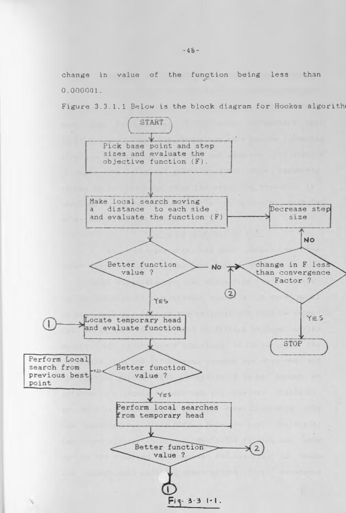
3.3. 1. 1 HOOKES AtU2 JEEVES ALQ.QB1THKL

This algorithm finds the minimum of a

multivariable, unconstrained function. The procedure L3 based on the direct search method proposed by Hookes and

Jeeves [12]. The algorithm proceeds as follows;

1) A base point is picked using the autocorrelation

function coefficients as estimates and the objective

function evaluated.

2) Local searches are made in each direction of

steps Xi, for each parameter value and then evaluating

the objective function to see if a lower function value

is obtained.

3) If there is no function decrease, the step size is

reduced and searches are made from the previous best

point.

-44-

4) If the value of the ^objective function has

k+1decreased, a "temporary head ”, Xi,o , i3 Located using

k*-l kthe two previous base points Xi and Xi ;

k*l k + 1 (k + 1) (k)Xi, o =Xi + a( Xi -Xi )

where i is the variable index - 1,2,3,....N

o denotes the temporary head

k is a stage index ( a stage is the end of N searches)

a is the acceleration factor, a> 1.5) If the temporary head results in a lower function

value, a new local search is performed about the

temporary head, a new head is Located and the value of

the function, F i3 checked. This process continues so

long as F decreases.

6) If the temporary head does not result in a lower

function value, a search is made from the previous best

point.

7) The procedure terminates when a convergence

criterion is satisfied (e.g when change in F is less

than a convergence factor).

For example in the evaluation of the optimum model par­

ameters of equation 3.2.2 (pp36) using 1008 hours of load

data, initial parameter estimates of 0.2 and 0.4t

obtained from the ACF were used as the base point.

These converged to optimum values of 0.06 and 0.85

respectively after 165 iterations in 1.5 minutes, with a

«

- 4 6 -

change in value of the function being les3 than

0.000001.Figure 3.3.1.1 Below is the block diagram for Hookes algorithi

pi 3•3 I • I .

-46J

3.3.2 PARAMETER ESTIMATES frND DIAGNOSTIC CHECKSOnce a model has been satisfactorily identified

and its optimal parameters obtained, the adequacy of fit

must then be assessed. If the model parameters are

exactly known, then the random sequence can be computed

directly from the observations, but when the calculation

is made with estimates substituted for true parameter

values as in this case, then the resulting sequence is

referred to as the ’residuals’, a which can be regardedt

as estimates of the errors.

3.3.2. 1 TESTS Of GOODNESS QE FIT.If a proper model has been chosen,then the

model residuals will not be different from white noise.

Model diagnosis involves estimating the autocorre­

lation function of the residual series a . A good modelt

is one where all lags of the residual ACF will be expec­

ted to be zero. For any kind of fitting of time series

models, it is obviously important to scrutinize the

residuals, i.e the differences between the observed and

the fitted values. With a computer it is no longer an

arithmetic nuisance to work out all observed residuals,

as well as their sums of squares. Notwithstanding that

the observed residuals differ from the real residuals,

important effects which may impair the fitting may show

up in the observed time series. For example, if there

are exceptional outlying observations, their existance

-4 7 -

will be revealed by a large residual term.

One of the tests of goodness of fit is the Port­

manteau lack of fit test. This uses the Q statistic to

test whether the entire residual ACF is different from

that expected of a white noise process [4).

If a fitted model is correct, then

3.3.2. 1k 2

Q=n fc[ACF(i)] i = l

is approximately distributed as X (Chi squared] distri­

bution with (k-P-Q-p-q) degrees of freedom, where n is

the number of observations used to fit the model and

ACF(i) is the autocorrelation function of the model

residuals at lag i.

Another test for goodness of fit is the evaluation

of the autocorrelation function of the residual series

and their 95% confidence limits. The sequence a ist

white noise with 95% confidence if______

[ACF(k )

th a5% confident

] < 2 ]/ i/N(ik T~

.+2 ^ [ACF( i ) ] ) ______3.3.2.2i = l

Estimates of the residual ACF which lie within plus or

minus two standard error of confidence are thus not

statistically different from zero at a 0.95 level of

confidence.

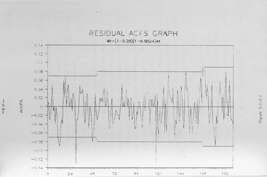
3.3.2.2 FITTED MODELS.168

The models 7 7 Z =(1-0.06B) (1-0.85B ) a168 t t

247 7 Z =(1-0.2B)(1-0.9B ) a

24 t t

3.3.2.2.1

3.3.2.2.2and

-40-

were tested for goodness of fit after having been tenta­

tively identified and their parameters estimated using

Hookes and Jeeves method.

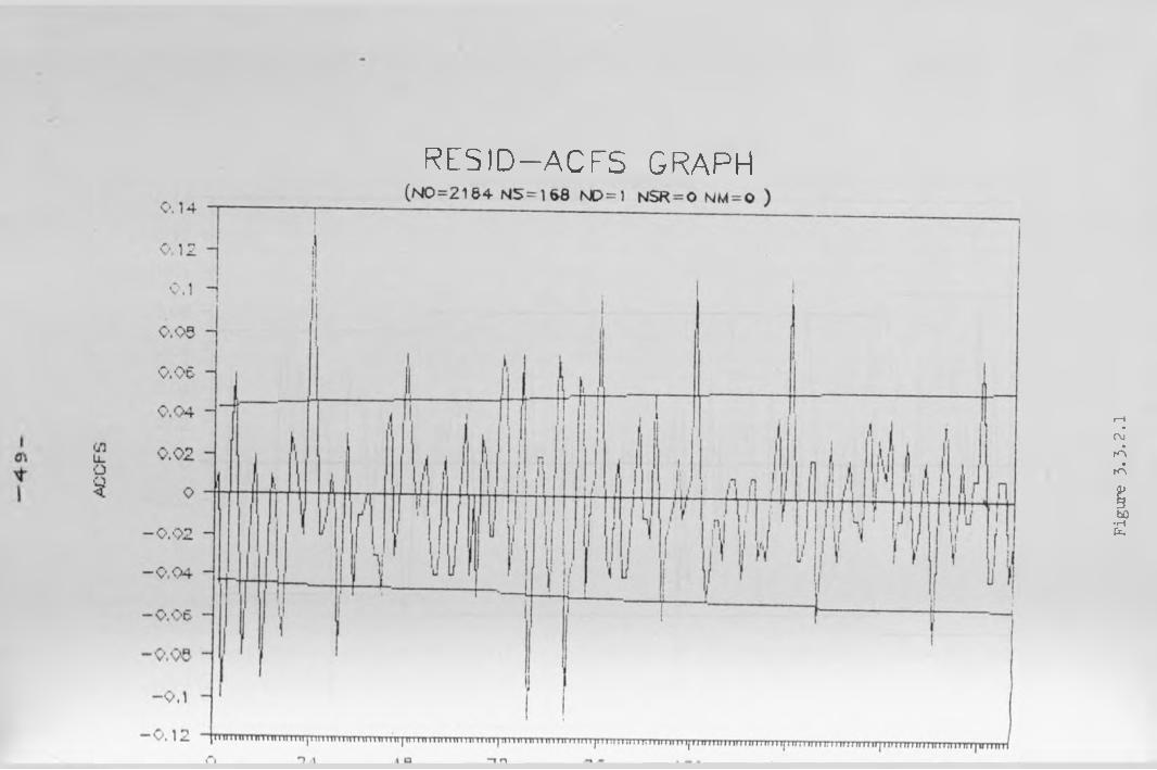
Figure 3.3.2. 1 shows the ACF of the residuals from

the model of equation 3.3.2.2.I and figure 3.3.2.2 shows

the ACF of the residuals of the model of equation

3.3.2.2.2. The chi-squared statistic (Q) was also eva­

luated for each model as well as the residual variance.

Residual variance is obtained by dividing the minimum

sum of squares function by the number of observations,n .

The below table shows some typical values of these

parameters.

! Model Typel1lll1»

Q statistic For n = 840

Percentagepoints ondistribution2.5% ! 5%1

ResidualVariance

Degrees of Freedom

! 7 7 Z =! 168 t ! 168(1-e B)(1-e B )a: i 2 t1

23.7

11131.5 128.91(111

143. 1 18

: 7 7 z = 11! 24 t 11: 24 27.2 31.5 128.9 179.5 18(1-0 B)(l-e B )a 11! 1 2 t 1_ i _

Table 3.3.2.1

Both these two models passed the diagnostic checks

using the Q statistic criterion. A careful scrutiny of

the autocorrelation function of the model residuals and

observation of the 95% confidence lines over a time span

RESID-ACFS GRAPH

Figure 3.3.2.1

»0tfll

•/]U-O'i

0.14

0.12 0.1

0.05

v. Ot

0.04

0.02

o

- 0.02

-0.04

-0 .06

-0.05

- 0,1

- 0.12

-0 .14

RESIDUAL ACFS GRAPHWt = (l-0.2B)(1 -0.9B24)At

O 24 ??■ 12; 1 &e 1S2

t

4? 1 44

Figu

re 3

.2.2.2

#\

-b 1-

of about 200 lags reveals that the model of equation

3.3.2.2.1 is a better fit than that of equation

3.3.2.2.2 since it has a lower residual variance and

it’s residual ACF graph has fewer and less significant

spikes at the 9b% confidence interval.166

The model V V Z =(1-0 B )(1-e B ) a is thus the 166 t 1 2 t

better model chosen for further development and analysis.

Analysis of figure 3.3.2.1 shows that there are sig­

nificant spikes at lags 2, 24, 48 and 72. These spikes are

multiples of 24 and the residual autocorrelations

decrease from lag 24 to 48 ,a similar decrease from lag

48 to lag 72 also being registered. These evolving

patterns in the residual ACFS shows that, there exists a

seasonal autoregressive term of degree 24 which was

overlooked at the identification stage and must now be

included in the model. The significant spike at lag two

also reveals the presence of a regular moving average

term of order two which should be taken care of at this

stage.Use is made of the notion of the iterative model

building strategy earlier mentioned of

identification, estimation and diagnostic checks, to

obtain an improved model. After diagnosis the below

model is entertained;24 2 168

(i-^B )V v <z =(i-e B-e b )(i-e b ) a3 168 t 1 4 2 t

3.3.2.2 .

-52 -

The parameters of this new mq_del were then evaluated

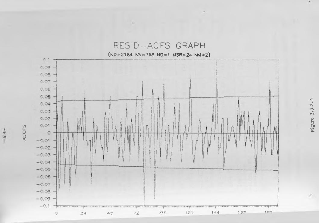
using the parameter estimation program.Figure 3.3.2.3 shows the autocorrelation function

estimated from the model residuals of the model of

equation 3.3.2.2.3 .There are no significant spikes at

the early or seasonal lags. The Q statistic for this

model is ( 20.4 ), which is not significant at the 0.05

level,as can be seen from table F in appendix. Scrutiny

of the residual ACFs graph also shows that there is no

significant departure from zero.

The final model chosen is thus;

24 2 168( 1- ^ B ) 7 7 Z = (1-0 B- e B )(l-e B )a . ______3 . 3 .2 . 2.4

3 168 t 1 4 2 t

The model of equation 3.3.2.2.4 is the selected

objective function for the Hookes and Jeeves

optimization program. This model is then incorporated in

the subroutine LEAST which is used by the main program

for evaluating the optimum model parameters.

Five weeks of load data (840 hours) for different

periods of the year was used in the evaluation of the

model parameters as summarized in table 3.3'. 2.2.

It can be seen from the table that the model

parameters vary within expected limits as the year is

spanned indicating the fact that the model chosen and

its parameters is quite a good representation of the

load process. The average values for the optimum model

\

AC

CF

V3

RESiO-ACFS GRAPH(N0^2184 NS = 168 ND=1 N5R^24 NM=Z)

O 24 4? 72 9 6 120 14-4. IP.**

Figure 3

.3.2

.3

-54

parameters over the considered periods are:

9 = 0.1, 0 = 0.85, j> - 0.1 and 6 =0.11 2 3 1

These are the values to be used for the load forecasting

process as the power load model has been completely

specified at this stage.

ThLa table shows ths optimum panamatar values Evaluated ,

!LOAD DATA ;SET PERIOD

OPTIMUM PARAMETER VALUES RESIDUALVARIANCE

CHI-SQUARED2

! (N=840) 0l

02 *3

04

(Sum of Squares /N)

X statistic ( k=2G0 )

! L-1 -87: t o: lb-2-87

0. 11 0.85 0.00 0.01 202.9 225.8

: 25-11-87 ! TO : 10-1-88

0.03 0.85 0.23 0.05 110.1 195.4

! 24-2-88 ! TO 1 22-3-88

0.11 0.83 0.05 0.06 124.48 208.9

1 6-4-88 : TO ! 10-5-88

0.27 0.89 0.01 0.07 168.3 176.6

J 18-5-88 ! TO I 28-6-88

0.05 0.87 0.18 0.08 141.9 163.9

! AVERAGE !PARAMETER 1 VALUES OVER ! PERIODS

0.11 0.85 0.09 0.06 149.5 194.1

Table 3.3.2.2

It has been pointed out [4] that a small variation in

the value of the model parameters does not affect the

accuracy of the load forecasting process as long as the

- b 5 -

right form of the model, has been identified. For example

a ten percent variation in the value of the parameters

does not affect the forecasts appreciably, as shown in

table 3.3.2.3 below.

ESTIMATED MODEL PARAMETERS FOR FORE­CASTING.

MEAN ABSOLUTE PERCENTAGE ERROR (24 HR) LEAD TIME FOR

OPTIMUMVALUE

10% INCREASE IN OPTIMUM PARAMETER VALUE

1096 DECREASE IN OPTIMUM PARAMETER VALUE

Hi 3.6 3. b9 3.62

02 3.6 3.84 3.4b

03 3.6 3.60 3.61'

64 3.6 3.60 3.61

Table 3.3.2.3»

The parameters could also be updated on-line if

there becomes available faster algorithms for parameter

estimation and on-line data acquisition methods. The

parameters can be updated off-line periodically, to see

whether they change appreciably as time goes on.

-56 --

CUAPTSB 4 ^FORECASTING.

4.0 INTRODUCTION.

One of the important aspects of a modeling process

is to put the identified model to use. In this case,the

identified power load model is to be used for load

prediction. A good model is one that provides accurate forecasts of the load and the forecasting abilities of

these models can be investigated by comparing actual

load values with the forecasted values.

4 1 IHE EQRECASTING ALGORITHM.The estimation stage of the model identification yields

24 2 168the model (1-0.IB )7 7 Z =(1-0.1B-0.IB )(1-0.85B ) a

1 168 t t___________ 4.1.1

as the best amongst the ones considered and since it

passed diagnostic checks, it is the final model to be used for forecasting.

Expanding the polynomial equation for the model and

solving for Z , the load value at time t, we have t

24 * 168 2 168(1-0. IB ) (1-B) ( 1-B )Z =(1-0.1B-0. IB H1-0.85B ) a

t t„ 4.1.2and further expansion gives

Z =Z +Z -Z +0.1(Z -Z +Z -Z )+at t-1 t-168 t-169 t-24 t-25 t-193 t-192 t

-0.1a -0.1a -0.85a +0.085a +0.085a _ 4.1.3t-1 t-2 t-168 t-169 t-170

- 5 7 -

Starting at a time t, the Load forecast L hours✓

ahead is given byZ{L)-Z +1 "Z +0.1(Z -Z +Z

t + L-1 t + L-168 t*-L-169 t*L-24 t+L-25 t+-L-193

+Z )*a -0.1a -0.1a -0.85at + L-192 t*L t+-L-1 t + L-2 t<-L-168

>0.085a ♦■0.085a _________ 4.1.-t + L-169 t<-L-170.

where a is the one step ahead forecast error.thus t

a =Z -£ (1).t+L t + L tt-L-1For example the forecast for a lead time of one

hour would be given by£ (1 )=Z *Z -Z -0.1(Z -Z -z *Z )- t t t-167 t-168 t-23 t-24 t-192 t-191

0.1(Z -£ (1))-0.1(Z -£ (1))-0.85(Z -Z (1))t t-1 t-1 t-2 t-167 t-168

+0.085 ( Z -Z ( 1 ) ) +0.085 ( Z -'Z (1)).___4.1.5t-168 t-169 t-169 t-170

Forecast equations for other lead times can be similarly

obtained by substituting the appropriate value of lead

time L and time origin t into equation 4.1.4.

It can be seen from the forecast algorithm that at

least 169 observations are required to start up the

forecasting process because of the regular and seasonal

differencing operations performed on the series (d=D=l

and s=l68).The seasonal moving operator also means that at

least 170 one step ahead forecasting errors are required

-58-

before an accurate forecast can be obtained. This in

essence means that a load forecasting data base of at

least 339 hours of load observations are required to

obtain any meaningful load forecast. It was found that

the load forecasting process stabilizes with about three

weeks of hourly load data. Three weeks of Load data (504

hours) was chosen as the size of the load forecasting

data bank, since it is also important to 3tore only the

minimum amount of historical data at any time to

minimize the computation time of the forecasts.

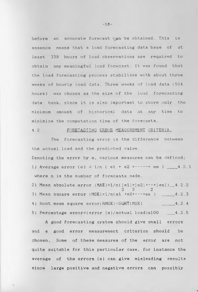
4.2 FORECASTING ERROR MEASUREMENT CRITERIA,The forecasting error is the difference between

the actual load and the predicted value.

Denoting the error by e, various measures can be defined;

1) Average error (e) - 1/n (el *■ e2 +---- + en ) ____ 4.2.1

where n is the number of forecasts made.

2) Mean absolute error (MAE)=l/n(!el!+!e2!+--+!en!)_4.2.22 2 2

3) Mean square error (MSE)=l/n(el <-e2 +-- -*-en ) _____ 4.2.3

4) Root mean square error(RMSE)=SQRT(MSE) _____4.2.4

5) Percentage error=(error (e)/actual load)xl00 __ 4.2.5

A good forecasting system should give small errors

and a good error measurement criterion should be

chosen. Some of these measures of the error are not

quite suitable for this particular case, for instance the

average of the errors (e) can give misleading results

since large positive and negative errors can possibly

\

-52 -

cancel each other out.

One of the best measures of the forecasting error

is the mean absolute error (MAE). Root mean square error

is also an acceptable criterion. In this study mean

absolute error measurement criterion is used

analysis of the forecasting results.

for

4.3 TREATMENT Of ANOMALOUS LOAD PATTERNS, During some days of the year,the load model fails

to describe the normal load. Such anomalous load

patterns occur during public holidays such as

Christmas, easter, labour day, independence day and others

that may be declared from time to time. These abnormal

loads could also occur due to unforeseen circumstances

like industrial strikes, power blackouts and

emergencies.

other

The large errors in a normal forecast of the

holiday loads tends to distort the model temporarily

causing further errors in the following normal days.

Holiday loads are considerably lower than normal weekday

loads but are mostly like neighbouring Sunday loads.

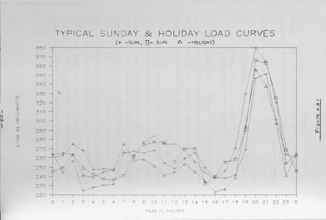
Figure 4.3.1 shows a plot of typical Sunday loads

compared with typical holiday loads. The graphs clearly

show that Sunday loads do not differ appreciably

holiday loads.

from

An analysis of the load patterns has shown that

loads of holidays are not necessarily the same,for exam-

\

IN

MEG

AW

ATT

S

Q<3

TYPICAL SUNDAY & HOLIDAY LOAD CURVES( + — S U N ., 0 - S U N ., A -H O L ID A Y )

-Sim­

ple a Christmas holiday tends to be similar to a pre­

vious Christmas holiday, but could be quite different

from a labour day holiday. It has also been found that

the neighbouring Sunday load to a particular holiday is

more similar to that holidays load than, say the load

of the last holiday observed.In order to avoid overestimating holiday loads.the

load forecasts for holidays are taken as the Latest

Sunday load readings recorded and for that particular

holiday, the system load readings are not entered in the

load forecasting data base, instead these values are

replaced by forecasts.Actual load readings are also replaced by forecasts

in the load data base in case it is not possible to

obtain the load readings for one reason or another for

example when there is a failure in the metering system.

4.4 LOAD FORECASTING RESULTSThe recursive nature of the load forecasting algo­

rithm enables the latest load reading to be used for

obtaining forecasts and this makes the forecasting pro­

cess adaptive in that as new load readings are obt­

ained, forecasts can be updated.

The output of the program gives the load prediction

for the next twenty four hours and the errors in the

previous hour’s forecasts.

\

-&2.-

One of the advantages of ,this model is that its

inherent structure allows the forecasting of weekend

loads with the same degree of accuracy as for weekdays.

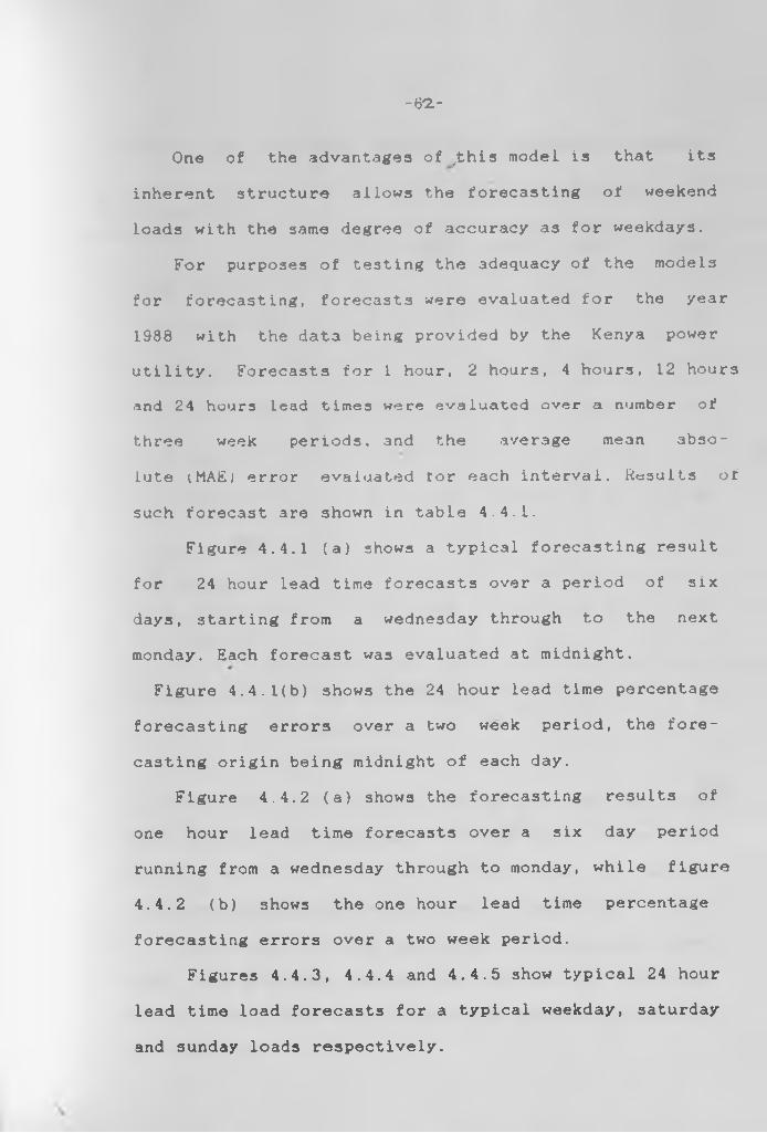
For purposes of testing the adequacy of the models

for forecasting, forecasts were evaluated for the year

1988 with the data being provided by the Kenya power

utility. Forecasts for 1 hour, 2 hours, 4 hours, 12 hours

and 24 hours lead times were evaluated over a number of

three week periods, and the average mean abso­

lute MAEj error evaluated tor each interval. Results of

such forecast are shown in table 4.4.1.

Figure 4.4.1 (a) shows a typical forecasting result

for 24 hour lead time forecasts over a period of six

days, starting from a Wednesday through to the next

monday. Each forecast was evaluated at midnight.

Figure 4.4.1(b) shows the 24 hour lead time percentage

forecasting errors over a two week period, the fore­

casting origin being midnight of each day.

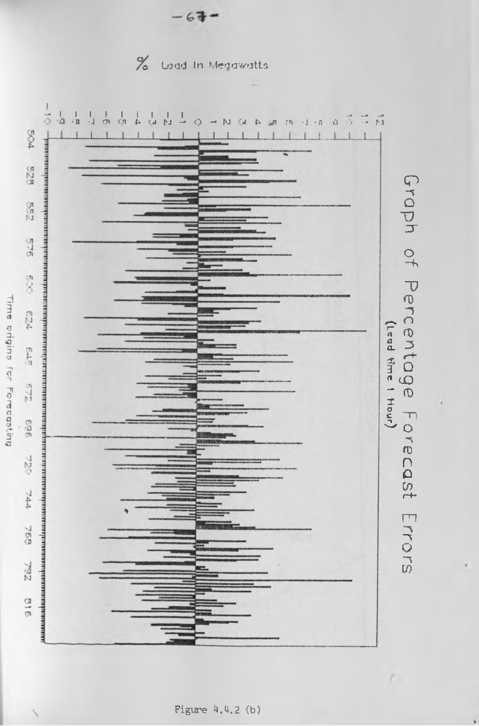
Figure 4.4.2 (a) shows the forecasting results of

one hour lead time forecasts over a six day period

running from a Wednesday through to monday, while figure

4.4.2 (b) shows the one hour lead time percentage

forecasting errors over a two week period.

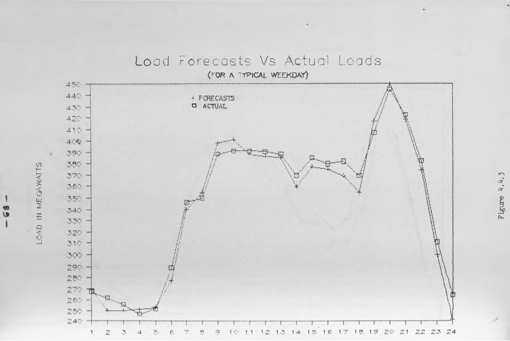
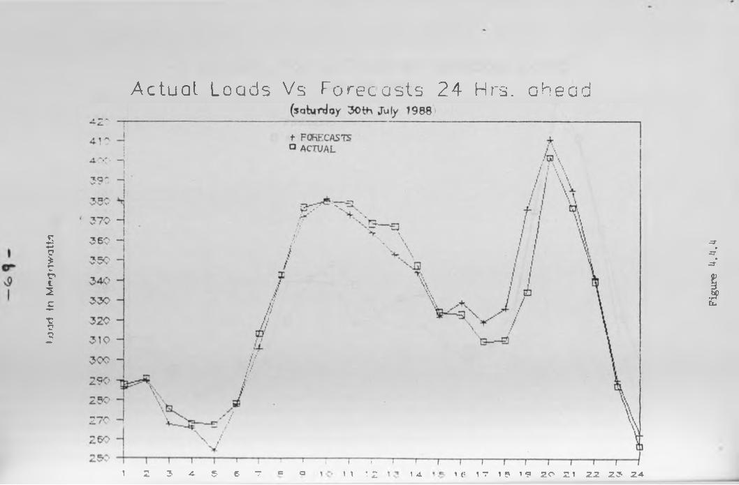
Figures 4.4.3, 4.4.4 and 4.4.5 show typical 24 hour

lead time load forecasts for a typical weekday, Saturday

and Sunday loads respectively.

-63-

AVERAGE MEAM ABSOLUTE PERCENTAGE FORECASTING

; PERIOD DURING ! WHICH FORECASTSI WERE MADE»»•

LEAD TIME OF THE FORECASTS

1HR(MAE)

2HRS(MAE)

4 HRS (MAE)

12HRS (MAE)

24HRS(MAE)

3.60! 29th June to•

! 2nd August 1988«

tl2.87 3.18 3.50 3.52

; 18th May toii 28th June 1988•1l

2.84 3. 10 3.53 3.52 3.71

24th Feb.toll! 29th March 881•li•ll

2.82 2.97 3.30 3.94 4.36

! THE AVERAGE ! MEAN ABSOLUTE I ERROR FOR ALL| THE PERIODS.1

2.84 3.08 3.44 3.66 3.89

AVERAGE LOAD OVER THE WHOLE PERIOD = 328.8 MW

Table 4.4.1

From the above table it can be seen that alL the

mean absolute forecasting errors are well below five

percent and it can also be observed that the errors

slightly increase with an increase in lead time.

The errors for one step ahead load forecasts ave­

rage to 2.8 percent showing the usefulness of updating

the forecasts every hour to obtain a better forecast for

the next hour.

\

Load

In M

egaw

atts

Graph of Feasts Vs actual Loads(Lead Time 1 -2 4 Hours)

Time Origins fo r Lead-tim es 1—24 Hours

Figu

re

Figure l (b)

U U I j a U J A J U J JV-J J i U I U U U J LLJ I I

SMb 36*1 b'9*1 tV/L OiTil 969 3*19 at’"9- J&J 009 9US 3'a‘b oZ'a T>a

> 2 - l i a u j ' j . p*»»i j o j )

s>(Ojvi3 a B n ^ u a o j i a d j.o L f d o j ^

•nOr i■l

am3

I<5>Ml

\

/

Load

in M

egaw

atts

A plot of “ orecasts Vs actual Loads(Lead tfme 1 hour)

Time origins fo r lead time 1 hour

Figu

re

Load In Megawatts

I- i I i I I I i I i - - -O <a •:» 'J <71 <.n h <J» N — <> — M <ji P> j\ n -J -n O O — f J

\ Figure 4.4.2 (b)

Graph of Percentage Forecast Errors(tcqd tune I Hour)

LOAD

IN M

EGAW

ATTS

Load Forecasts Vs Actual Loads( r0R A TYPICAJ_ WEEKDAY)

Figure

^.4.

3

l/jo

rl

In M

©«g

»iw

att,

i

Actual Loads Vs Forecasts 24 Hrs. ahead

1 2 3 4- 5- 6 7 = a I I ! 2 U 1|< |7 I P 19 2 0 21 22 20* 24

Figure iJ.iJ.iJ

Lood

In Me

gawo

tt-B

\

T," - —I?ic -- v —V v

-

Z p,-.

It7'- -i

7 4..- —20" - 7 n,-

z. 1 v

*--E

Forecasts f or a 'ypical Sunday Load(Z4th July 1988)

— ±

*»*►-4--

i--- r4.

rf

* FCKECASTS 0 ACTUAL

/ /

/ d

..cf u' +

Tn

.a-.—a.\ Jsf TS

i--- 1--- r10 11 1

1--- T10 14. 1 «• 16 17 18 1 ? 20 21 20 24

/

Leod *imr in hrs(ffcaBt origin OO hrs.)

Figure

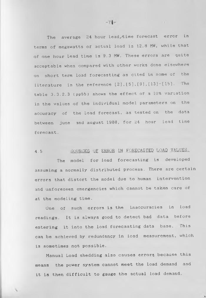
The average 24 hour Lead-time forecast error in

terms of megawatts of actual load is 12.8 MW, whiLe that

of one hour lead time is 9.3 MW. These errors are quite

acceptable when compared with other works done elsewhere

on short term load forecasting as cited in acme of the

literature in the reference 12],[5] ,[9],[13]-[151. 1he

table 3.3.2.3 (pp5b) shows the effect of a 1U% variation

in the values of the individual model parameters on the

accuracy of the load forecast, as tested on the data

between june 3nd august 1988, for 24 hour lead time

forecast..

4.5 SOURCES QE ERROR W FORECASTED LOAD VALUEDThe model for load forecasting is developed

assuming a normally distributed process. There are certain

errors that distort the model due to human intervention

and unforeseen emergencies which cannot be taken care of

at the modeling time.One of such errors is the inaccuracies in load

readings. It is always good to detect bad data before

entering it into the load forecasting data base. This

can be achieved by redundancy in load measurement, which

is sometimes not possible.Manual Load shedding also causes errors because this

means the power system cannot meet the load demand and

it is then difficult to gauge the actual load demand.

-T2L-

System frequency management can be another source of

error. Sometimes the system frequency deviates from the

required normal value and this could lead to errors in

knowing the actual load demand, for example in the Kenyan

power system every 0.1 hertz change in system frequency

is equivalent to about 5 megawatts change in electricity

demand.

The frequency deviation occurs mostly where utilities

are interconnected and there is no proper co-ordination

between the various control centers.

The load management program of ripple control of

domestic hot water heating systems,irrigation pumps in

farms and street lighting control also create errors in

forecasting because some of these installations are

manually operated by the power system controllers who

normally put them on at their discretion. An automatic

switch on and off system which responds to the system

load demand levels would alleviate this problem.

4.6 AREAS QZ POSSIBLE IMPROVEMENT■

One of the improvements that could be made to

this forecasting process is to model individual major

load buses and then using optimal control techniques to

combine the models for forecasting. These can only be

done subject to the availability of hourly load readings

for these nodes. This will be possible for the Kenya

system once the SCADA system of control which is

currently under Installation Is Implemented.

Another area that needs serious and thorough study

is the treatment of holidays and special day3 load

forecasts. This study ignores the loads for holidays and

instead replaces them in the load data base by their

forecasts. A comparative analysis found that the loads

on a particular holiday are quite similar to the loads

on a neighbouring Sunday. It was also discovered that

particular holidays are similar from year to year if

they occur on corresponding days such as the easter

holiday, for example. With good data management

techniques, a solution to such holiday problems can be

sought.

Erroneous load readings is one of the greatest

sources of forecasting errors and if many could also

lead to a poor model choice. A lot of work is currently

going on, on ways and means of bad data detection and

correction for power system state estimation. Some of

these techniques could be put to use in the load fore­

casting problem. At the rudimentary level,there should

be a redundant load measurement system that checks the

loads before they are used for forecasting. The effect

of the use of statistical tests to detect outliers in

load readings before forecasting as an improvement to

load measurements can also be a subject of further

investigation.

5.0

CUAETEB 5

CONCLUSIONS^

This study set out to develop a mathematical

model that describes the daily pattern of electricity

consumption in Kenya. The model was then to be used for

forecasting the load demand for a period ranging from

one hour to twenty four hours ahead.Using time series analysis techniques, an auto-

regressive integrated moving average model of four para­

meters has been developed. The model parameters were

estimated using Hookes and Jeeves optimisation

techniques. Six weeks of system hourly load data was

found adequate for model development.

Several tests were done at different times of the

year to verify that the model predicts accurately and

consistently. A continuous three week load forecast was

done for each of the testing periods for different lead

times and forecasting origins.

It has also been pointed out that the model develo­

pment is based on the stochastic nature of the load

process and no weather variables have been included

because weather inputs could lead to double forecasting

errors if there are no adequate weather records. In any

case, in Kenya there is very little weather sensitive

equipments installed because of the country’s location

within the tropics.

The Load forecasting process is hourLy adaptive with

Low computer memory requirements since the program onLy

needs to store three weeks of hourLy Load data to be

able to make a forecast. The hourly updating of the load

forecasts minimizes the effects of uncon3idered weather

variables.

This studys forecasts gives mean absolute perc­

entage errors of less than five percent for 24 hour Lead

time forecasts and less than three percent error for one

hour Lead time. These results are quite accurate

compared with other results obtained elsewhere for short

term Load forecasts. These results should go along way

in enhancing the efficient monitoring, operation and con­

trol of the Kenyan power system.

- 7 6 -

REEERENCESi S'

1. M. A.Abu-El-Magd and N.K.Sihna, "Short term load demand

modeLing and forecasting" A review, IEEE Trans, on syst­

ems, man and cybernetics; vol. SMC-12, no 3 pp 370-382

May-June 1982.

2. R.Campo and P.Ruiz, Adaptive weather sensitive short

term Load forecasting", IEEE trans. on power systems vcL.

PWRS-2 no 3 August 1987.

3. J.Toyoda, M.Chen, Y.Inouye, "An application of state

estimation to short term load forecasting", IEEE Trans.

PAS 89 no 7 Sep.\0ct. 1970 pp 1678-1688.

4. G.E.Box and G.M.Jenkins, Time Series Analysis, Forecas­

ting And Control; San Fransisco: Holden-day, 1970.

5. M.T.Hagan and Suzanne Behr, "Time series approach to

short term load forecasting", IEEE Trans.on power systems

vol. PWRS-2 no 3 August 1987.

6. M. Hagan and R.Klein, "Identification techniques of Box

and Jenkins applied to the problem of short term load

forecasting", IEEE power Engineering society meeting

July 1977 paper no A77 618-2.

7. P.D.Mathewman and H.Nicholson, "Techniques of load

prediction in the electricity supply industry", Proceed­

ings of IEE vol. 115 no 10 1968.

8. E.D.Farmer and M.J.Potton, " Development of on-line load

prediction techniques with results from trials in the

South-West region of the CEGB", Proc. IEE Vol. 115 1968.

\

9. W.R.Christiaanse, "Short term Load forecasting using

general exponential smoothing , IEEE Trans. PAS 90 March-

April pp 900 1972.10. M.Plosser, "Short term load forecasting and seasonal

adjustment", Journal of American statistical association

1979 pp 15.11. D.J Wilde and C.S Beightler. Foundations of optimizat­

ion Prentice Hall, N.J. 1969.12. J.C .Kuester and J.H.Mize, "Optimization Techniques

With Fortran, Mcgraw Hill, 1976.13. M.A.Abu-El-Magd and N.K.Sihna, "Univariate and multiva­

riate time series techniques for modeLing and forecasting

short term load demand", IFAC symposium on theory and

application of digital control, India, Jan. 1982, paper

no 5-4, pp 329.14. M.S.Abou-Hussein and M.S.Kandil, "An accurate model for

short term load forecasting', IEEE Trans. PAS 1981 pp 41o8

15. B.Krogh, E.S.DeLlinas and D.Lesser,"Design and implemen­

tation of an on line load forecasting algorithm", IEEE

Trans. PAS pp 3280 1982.

BIBLitQQRAfHY:

1. K.Srinivasan and R.Provonost, Short term load for­

ecasting using correlation models", IEEE trans. PAS 94

no 5, 1975.2. P.C Gupta and K.Yamada. "Adaptive short term load fore­

casting of hourly loads using weather information". IEEE

Trans. PAS 91 no 5, Sept\Oct. 1972.3. P.Stoica, "Tests for Whiteness", IEEE Trans. Automatic

control vol.22 no 6 pp 992-993 1977.

4. D.C.Hamilton and D.G.Watts, "Interpreting partial

autocorrelation functions of seasonal time series models

Biometrika 1978 vol. 6b pp 135 140.

5. H.Akaike, "A new look at stochastic model identifica­

tion", IEEE Trans. Automatic control vol. AC 19 pp 716-

732, 1974.6. J.Murdoch, Statistical Tables For Science And Engi­

neering, Me Millan, pp 17.7. J .A .Greenwood and Hartley, Guide To Tables in

Mathematical Statistics, Princeton University press

1962, pp 140.8. S.M.Simpson, Time Series Computations In Fortran And

Fap, Addision Wesley.9. W.Gilchrist, statistical Forecasting, John Wiley and

sons, 1976.

APPSMEUL. 'The load modeling and forecasting procedure has been

implemented as five computer programs,all written in

standard Fortran 77 Language and developed on an IBM

personal computer.The programs TEST is for model identification and it

evaluates the autocorrelation functions of various

transformations of the series such as differrencing

.natural logarithmic transformation as well as

calculating the 95% confidence intervals.

The programme PCF is also a model identification

programme which takes the autocorrelations as it’s input

and evaluates the partial autocorrelations up to the

desired lags.Programmes SHADD and DIAGN are for parameter estima­

tion and diagnostic checks. These give the values of the

optimum model parameters,their residual variance,the

autocorrelation function of the model residuals as well

as the Chi-squared statistic (Q).The final programme FCA5T is the load forecasting

programme that allows load prediction for a lead time of

one to 24 hours,as well as giving the values of the mean

absolute percentage errors of the forecasts and the

average load values over the forecast period.

The next couple of pages contain a user manual and a

print out of the program listings.

«*

LOAD FORECASTING PROGRAMS LLS£B MANGAI^The complete short term load forecasting algorithm

is implemented as five computer programs which are tor

model identification, parameter estimation. diagnostic

checks and load forecasting.These program^ aro coded in standard Fortran 77

language and are compiled using the RMFORT compiler that

requires a maths co-processor 8087 to run. A necessary

editor that is used is the Turbo Pascal editor which is

used for fortran file creation 33 well as the creation

of data files. Other editors such as the Wordstar can

also be used for data file creationAll the programs are contained in a single 3.5 or

three 5.25“ diskettes and they can all run on an IBM

compatible machine which has an 8087 maths co-processor.

Once the diskette is inserted, all that one needs to

type is the command README and a summary of each of the

programs and the directories where they are available

will be given. One is then able to chose the particular

program of interest.

PROGRAM TEST,.

The compiled version is TEST.EXE. It calculates

the autocorrelation functions to the desired lag, and

for this particular case the lag is limited to 500 but

this could be increased by dimensioning the ACOR(J)

array. The input data required for the program is the

- A . 0 -

past hourly load series observations which has to be

entered through the keyboard into a data file named

LDATA. This program handles upto 2200 hours of load

data, which can also be increased by proper dimensioning

of the X array.The screen inputs required for this program are;

1) The number of load series observations

2) The maximum lag of autocorrelation required

3) The seasonal period

4) The degree of regular differencing

All the above inputs are through appropriate screen

prompts. The results are obtained from a file ALPS which

lists the autocorrelation function coefficients versus

their lags in a tabular form as well as their 95t

confidence intervals.

PBggBAEI E££L_The compiled version is PCF.EXE. Execution of PCF

always follows that of TEST programs since it obtains

it’s input from the output of TEST. The only input

required here is the maximum lag of the partial

autocorrelation desired. In this program it is limited

to 75, but it’s value could be increased by dimensioning

the array P accordingly if there is sufficient memory.

The output of the partial autocorrelation

coefficients versus the lags in tabular form are

obtained from the file PCFOUT.

- A. I -

PROGRAM SHA.P.D,''The compiled version is SHADD.EXE. It's execution

requires the use of past hourly load data, to be entered

in a ’LDATA’ file before execution of the program. The

array size for this particular program allows upto 2200

hours of load data for model parameter estimation.

Other inputs for the program which are entered on

the screen through prompts are;

1) Number of model parameters to be evaluated

2) Initial parameter estimates3) Initial step sizes for changing parameter estimates

4) Number of hours of load series observations5) Maximum lag of autocorrelation required for

diagnostic checks.

6) Seasonal period

7) order of AR and MA parameters

8) Choice of whether series is to be Log transformed or

not.

9) Convergence criteria.The results obtained from a file PESTIM gives the

optimum parameter values, the minimum sura of squares

function, the residual variance, the number of

iterations as well as generating the residual series, at

corresponding to the optimum parameter values. The at

series are used as the input to the program DIAGN for

evaluating the ACF of the residuals for checking for

goodness of fit. The objective function for this model

parameter evaluation program is developed in the

subroutine LEAST1.

PROGRAM DIAGN.The compiled version is DIAGN.EXE. It is run only

after executing the program SHADD which generates the

residual series a , which it writes into a file RESIDt

which is then used by the DIAGN program to evaluate the

autocorrelation functions of the residuals. It also the 2

X statistics as well as the 95% limits of the ACFS. All

these results are obtained from a file ACFS.

PROGRAM FCAST-This is the program that generates the required

hourly load forecasts. To start off the forecasting

process, a load data base of the most recent 504 hours (

3 weeks of hourly load data ) is entered into a data

file, ’LDATA’. This data file can be created by the

turbo editor. Once this has been done, a decision can

then be made of how often the forecasts are required.

A policy of generating a forecast either once a

day (every 24 hours) or every one hour is recommended to

avoid a lot of confusion. If possible load forecasts

should be done every one hour, since the hourly updating

makes the forecasting process more accurate.

Before one performs a forecast, there will be a

screen LOGO of invitation to a forecasting session

►

asking for the following information to be entered on

the screen;1) The last time a forecast was made (hour,day,year)

2) The present hour and date3) The number of hours that have elapsed since the last

forecast was made.4) If the forecast is done hourly, then the load

reading of the previous hour is required, otherwise if

the forecast is done once a day., then the latest J4

hours of hourly load values will be required before a

forecast is made since this is a time series process.

The forecasts are then generated and the results

obtained from the file FCOUT which lists the lead times

versus the Forecasted load values. The error in

forecasting the previous hours load is also generated.

Once the forecasting process is started, the load data

file is updated automatically, through a recursive

process as the forecasting process continues.

GRAPHS.

All the outputs of the above programs are in a tabular

form which makes it quite easy for graph plotting. The

LOTUS 123 utility is used for generating and plotting

the graphs.The 123.EXE option is used to invoke the worksheet menu.

The "import " option on the menu is used to transfer the

- A . 4 -

results file, { whose data is-to be plotted ) into the

worksheet. The graph can then be easily generated and

viewed on the screen using the graph commands of the

lotus software. The graphs can be plotted on paper using

the "printgraph" option of the software, through either

a text printer or a graphic plotter.

- A ■ o **

-FQSRAWtE TE3T: {creating storage apace ‘or arrays:Array < scor*? the load aeries: observation ,array ACGR is for storing the aufcpcorrelations.array: SFX is for holding the differenced Load observe.and r is ‘or: standard error evaluations]

3I*ENS 1 ON <12200).ACC?i:0>:\CF<'2200».'<«500)•NITEll.l)

1 FQfiHAT: •i) THIS PRQSMHHE IS FOR "ODEL IDENTIFICATI0N AMD IT CALCS LATE3 THE AO TO C OR fi EL fi TIC NF UNC T10 N COEFFICIENT. / j

• *RTE(1,I) INPUT Tho timber of Load series observationsREMU.HLXXRITE11,*;'INPUT Tne *as:»n lag of autocorrelation required READ f 1,11HLASr- lTE >.• INPUT The sessi'ui :eriod READ *, * • NS•:!rE.i.i! :n=Ut TNe oegrw of 'eguiar differencing READ 11,1 no if N0.8T,2‘ tiENlAITEtl.tl'FQR THIS PR08RANHE DE8REE OF nQN-SEASONAL D!?=t?E*»C!N6 1 IS jPTO OF IE5 2 ONL'f ELSEAprs *,2j:?WAri«, THE INPUT 3ATA FOR 'HE LOAD-SERIES ;It) IE TPOUSH ’L3A •»' FILE WHOSE CONTENTS IAN 3E AMENDED APPR'3PR!AT£LV USING THE 1 ■•-roo cascal *oitcra •RITE M)-'T^ATm , .Ajr C-.S :;*c..TiT;CNS and *“EN obtain *-E RESULTS from *■€ FILE 'AC?3* AFTER THENORO cress a key :o continue* :r 'A * 4 WEARS CN THE SCREEN.

c { =~======ooe(ung input data fiies================5

IREN;5,RILE* '.DATA ,STATUS* OLD')5PEN!4,FILE*'PCFIN'.STATUS*1 OlD >

c [ l/=No of observations of load data tne series C NXLAS=*axi*u« lag of autocorrelation function coeffs.2 N3*degree of seasonal differencing (D)C NC=Begree of non-seasonal differencing (d) }

READ{5, t)(X(I)rI=l>LI)CLOSE i 5«STATlJS*' * EEP j:***=**====*== perforfing natural logarithmic data translationDQ 10 1=1,LX<(I)=AL06(((I)|

10 IDNTINIJEc **=***=opening output raSUlts file==========

:PENi7.FILE=*CF5 ,STATUS*'OLD )JHAi*HiL4S+2 IF (NS.6E.lj THENCALL DIFF(X,LUS,NS,OFX!IF IND.SE.t) THEN CALL DIFFIDFX.LS.LD.ND.DFX)IF 'ND.Efl.2j THEN CALL DIFF(DFX,LD,LB,ND,DFX)CALL RE1AV(DFI,lB,<AV6)CALL FCRAC(DFX,LB,MXLA6.AC0R(J))

ELSECALL REHAV(DFX,LD,XAV6)CALL FORflC(OFXlLOlf1XLA6,ACOR(J))

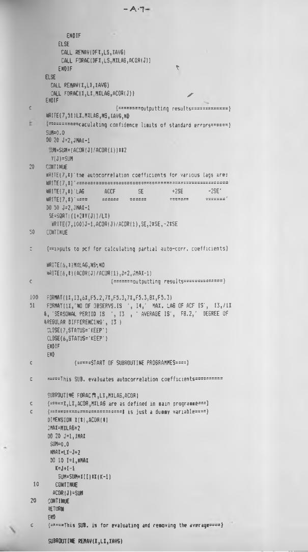
- A-l

ENDIFELSECALL aOWV(DFT,LS,XAVS)CALL FORAC(DFI,LS,HXLA6,ACGR(J))EN01F *

asECALL REMAV(X,LX,XAV6)CALL FQRAC(X,LX,HXLA6,AC0R(J|) ,

ENSIFc {:==s==r=outp1Jtting resuits=============>

NRITE(7,5l)LI.NXLAG,NS,XAVG,NDt""===”=caCuliting confidence lints of standard errors======)StIW.O00 20 J=2,JHAI-1 :UH=SUH+ (ACOR (J)/ACOR(l))112 Y!J)=SUN

20 COAT I WJ£»R!TE(7,l)'tne autocorrelation coefficients for various lags are:NRITEI7,t)' ===™=ss»======s==»»========«=======sWITE(7,I)LA6 ACCF SE +2SE -2SE*NRITE(7,I)'=== ====== ====== ======= “====='DO 50 J=2,JHAI-1 SE=SQRT((1*2»Y(J))/LX)*RITE(7,100)J-1,AC0R(J)/AC0R(1),SE,2ISE,-2JSE

50 CGMTINUE

: (“inputs to pcf for calculating partial auto-corr. coefficients)

«iTE(6,l)f1<LAG,NS*,«tDnRI7E(4,IS(AC0R(J)/AC0R(l),J=2,JHAX-1)

c (=======outputting results111"”—-1” 1}

100 F0R*WT(1X,I3,6X,F5.2,7X,F5.3,7X,F5.3,8X,F5.3)51 FORMAT(IX,XO OF OBSERVE.IS ',14,' RAX. LAG OF ACF IS', 13,/IX

i, 'SEASONAL PERIOD IS ', IJ , ' AVERAGE IS', F8.2,' DEGREE OF MEHJLAR DIFFERENCING', 13 )CLOSE(7,STATUS5'KEEP')CLOSE(6,STATUS*'KEEP')ENDIFEND

c (=====START OF SUBROUTINE PROGRANNES====)

c =====This SUB. evaluates autocorrelation coefficients==========

SUBROUTINE FORACfX,LX,«XLA6,AC0R) c {====X,LX,AC0R,NXLA6 are as defined in earn prograiae===)c {::====rr=rr===r=s=====si==| 15 just a duaey variable====)

DIMENSION X(t),ACOR(I):«AX=HXLA6+2 DO 20 J=l,JHAI 5UN=0.0 NHAX=U-J+2 DO 10 I=1,NNAX K=J*I-1SUH=SUN+I(I)»X(K-1)

10 CONTINUE ACOR(J)=SUH

20 CONTINUE RETURN END

c (=====This SUB. is for evaluating and retoving the average™=)SUBROUTINE RENAV(I,LX,XAVG)

A ' 8

DIMENSION X(f) SU«=0.0DO 10 1*1,LIsn*sm+x(i)CONTINUE10

20

c

10

XAVS=SUH/LI DO 20 1=1,LII(1)3X(I)-XAV6 y

CONTINUE RETURN END""for perfoeing seasonal 4 non-seasonal differencing of series SUBROUTINE 0IFF(1,LX,LS,NS,0FT)DIMENSION X(I},DFX(t)LS=U-NSDO 10 1=1,ISOFX(n*X(I*NSH(I)CONTINUEENDEND

\

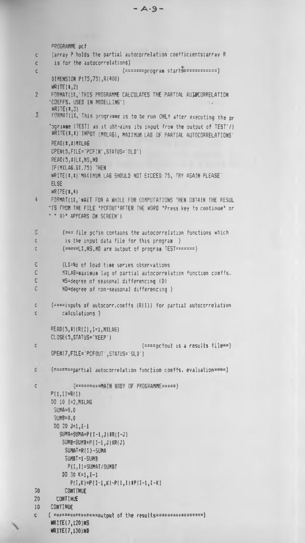
- A - 3 -

PROGRAMME pcfc [array P holds the partial autocorrelation coefficientssarray R c is for the autocorrelations)c {====="proqra« start £===========>

DIMENSION P(75,75),R(400)MRITE(t,2)

2 FORMAT(IX,'THIS PROGRAMME CALCULATES THE PARTIAL AUJNCQRRELATION •'COEFFS. USED IM MODELLING')»RITE(l,3)FORMAT(II,'This prograne is to he run ONLY after executing the or*oqra«*e (TEST) as it obt-ains its input fro* the output of TEST'/) *RITE(t,t)' INPUT (MXLA6), HAH HUH LAG OF PARTIAL AUTOCORRELATIONS' READ(*,t)MXLA60PEN(5,FILE='PCFIIT,STATUS2'OLD')READ(5,*)LX,NS,N0 IFINILAG.ST.75) 'HEMWRITE(«,»)'MAXIMUH LAS SHOULD NOT EXCEED 75, TRY AGAIN PLEASE'ELSE*R!TE(I,4)

4 FORMAT(IX,'MAIT FOR A NH1LE FOR COMPUTATIONS THEN OBTAIN THE RESUL*TS FROM THE FILE ‘PCFOUT1AFTER THE WORD ‘Press key to continue* or * ‘ A>* APPEARS ON SCREEN')

{=== file pcfin contains the autocorrelation functions which c is the input data file for this progra* )c (=~=LX,NS,ND are output of progra* TEST=======}

C {LX=No of load ti*e series observationsC NXLA6=*axiau« lag of partial autocorrelation function coeffs.C NS=degree of seasonal differencing (D)C ND-degree of non-seasonal differencing }

c {====inputs of autocorr.coeffs (R(I)) for partial autocorrelation c calculations }

REA0(5,t)(R(I),I=l,MXLA6)CLOSE(5,STATUS*'KEEP')

c [====pcfout is a results file— }0PEN(7,FILE= PCF0UT' ,STATUS='OLD*)

{"“ —partial autocorrelation function coeffs. evaluation=— =}

c B00Y OF PROGRAMME—™}P(l,l)-R(l)DO 10 I=2,MXLAG SUMA=0.0 3UMB=0.0 DO 20 J=1,1-1 SUM A=SUMA+P (I -1, J) IR (I - J)SUHB=SUMB+P(I-lfJ)tR(J)3UMAT=R(I)-SUMA SUMBM-SUMB P(I,I)=SUMAT/SUMBT

DO 30 K=1,I-1P(1,K)=P(I-1,K)-P|1,I)IP(I-1,I-K)

30 CONTINUE20 CONTINUE 10 CONTINUEc { ==is==5s:srrs==soutput of the results1—=—==—— ——=)

NRITE(7,120)NS NR1TE(7,130)ND

- A - l o -

NRITE(7,50!MLA6NRITE(7,55)

c ===s====“====evaluating confidence lieits of the estimatesc ==========r==gE 15 the standard Error===*=*=—”=========

SE=SQRT(1.0/LX) t*RITE(7,I)' LA6 PACCF SE'NRITE(7,I)'~« ====== ===='

c {=====P(I,I) is the partial autocorrelation at lagDO 60 I=1,HXLAS MRITE(7,100)I,P(l,I),S£

60 CONTIMUEC { :sjs*3«:::;s:ss Outputting results— 38*3******3235™ 22*}100 FORMAT(1X,I3,6X,F5.2,7X,F5.3)120 FORMAT(IX,'SEASONAL PERIOD OF ORIGINAL SERIES IS , 13)130 FORMAT(IX, DEGREE OF NON-SEASONAL DIFFERENCING IS , 13)50 PQRHATI1X, NATIHUH LAB OF PARTIAL AUTOCORRELATION COEFFS IS 13)55 FORNAT(IX,'THE PARTIAL AUTOCRRELATION COEFFICIENTS FOR VARIOUS LAS

tS ARE: ■)CLOSE(7,STATUS 'KEEP')ENDIFENDEND

- A-11 -

PRQ6RAHE 5HA0Dc This program is for model estimation using Hookes and Jeeves c '•on-linear optimization nethod.

dimension EPS(10),RK(10),Q110),QQ(10),W(10) *d imension X(2200),D12200),E(22001,A(2200) anted,21)

21 FormatllX,101,'THIS PROGRAMME IS FOR ESTIMATION OF flODEL PARAMETER*S7,1QX , ' )Uritel1,1)'INPUT M,The No of model parameters'Readd, OUST AGEdrited,t)'INPUT THE INITIAL PARAMETER ESTIMATES'Readd,»)(RK(II),11=1,NSTAGE)Nrited,!)'INPUT INITIAL STEP SIZE INCREMENTS FOR THE PARAMETERS ' Readd,»)(EPS(M),JJ=1,NSTAGE)idritef*,t)'INPUT LX(no of Load values),MXLA6(Lag of ACFS required) ‘,NS(seasonal period)'Readd,t)LX,MXLA6,NSNrited,*)'INPUT NSRIOrder of AR oarameter) .NMIQrder of 2nd MA Par ’ameter) 'Readd,DNSR.NH«rited,»)'IF LOAD SERIES IS LOSSED ENTER (1),OTHERWISE ENTER (0)’ Readd,t)L8

c ============================t_D AT A file contains input load seriesOpen (5,FILE3'LDATA',STATUS1' OLD')Read(5,*)(X(J),J=l,LX)Close(5,STATUS3 KEEP')

c ===================perfor»ing natural logarithmic transformationIf (L6.EQ.1)THEN do 11 1=1,LX X(I)=AL06(I(I))

11 continueelsedo 12 1=1,LX X(I)=X(I)

12 continue end ifopen(7,file='PESTIH',status3 OLD') open(6,file= RESID‘,status3 OLD')

c { IPRINT =1 means intermediate results are printed,and mhen=0 then c only final results printed.c maxk is the number of function evaluatons before the program isc terminated.c NKAT is the number of times the step size is decreased beforec programe terminates,c ALPHA is the acceleration factor,c SETA is the fraction by mhich the step size is decreased,c EPSY is the difference in function values before final resultc is accepted.c ND is the degree of regular differencing. )

c ==============inputting the programme constantsIPRINT=0NAXK=500NKAT=20ALPHA31.0BETA=0.5EPSY=0.0000001ND=1

%c ======================START OF MAIN PROGRAMME1333333333333333333

\5D30.0

- A M I

20

30

40

5045

61

10

401

?0

Cc201

513613

58

55

60CC

Urite(7,10)Foraatlll'lOI, HOOKES 4 JEEVES QPTIHIZATIQN ROUTINE')Nrite(7,20) ALPHA,BETA,HAXK.NKATForiat(//,21,' INPUT PARAHETERS*,/,21,'ALPHA5' ,lp.2,4I,' BETA5' ,F5.2 *,41,'ITHA15',I4,41, NKAT5*,13)Hrite(7,30)NSTA6EForiat(/,21, NUMBER OF VARIABLES5',13)Hrite(7,40) f

For«at(/,21,'INITIAL STEP SIZES')do 45 1=1 ,Nstaqe_ TSSWr*Continue

( , 12,*)=',F8.4)

*nte(7,61)EpsyFor»at(//,21, ERROR IN FUNCTION VALUES FOR CONVERGENCE5',E16.8> Call DIFF (1,L1,LS,NS,1)Call DIFF (1,LS,LD,ND,1)FFLA650Do sOl I5l,Nstaqe 9(I)5RK(I)N(i;=o.o

Continue*at50

1=0<count50Nbest5N(NstagelCall LEAST1(L1,1,NS,ND,E,D,A,RK,NSTA8E,SUH,NSR,LD,H,NH)Kkl=Kkl+l30=SUf1IF i KK1.£Q. 1)QD=5UM IF(KKI.EQ.1)8Q TO 201 IF(80.6T.QD)KFLAG=1 IF(BO.LT.QD)0D58O

==================5Establishinq Pattern Direction =™r=========sDO 55 I=1,NSTAGE 3 S ( I ) = R K ( I )

T3RK5RK(I)RK (I)=RK(I)+EPS(I)CALL LEAST1(L1,I,NS,ND,E,D,A,RK,NSTAGE,SUH,NSR,LD,H,NH)KKl^KMN(I)5SUHIF(N(I).LT.9D)6Q TO 58 «(I)5RK(I)-2.0IEPS(I)CALL LEAST1(L1,1,NS,ND,E,D,A,RK,NSTA6E,SUH,NSR,LD,!1,NH)ttl= ttl* lN(I)=SU«IF(N(I).LT.QD|G0 TO 58 RK(I)5TSRK IFU.E9.DG0 TO 513 N(I)=N|I-1)GO TO 613HUDBOCONTINUEKCOUNTU+KCOUNTSO TO 55GD5N(I)M(I)5RK(I)c o n t i n u e

IF (IPRINT)60,65,60 NRITE(7,100)KK1

= = 5 5 5 = = 5 5 5 ” 5 S * = f t p c o r d i n n R p t n n n c a 1 I n r a t i n n M w m m n u m i i

- A - 13-

NRITE(7,102)4RITE(7,207)(RK(I),I=1,NSTA6E),QD

C=====Tests to detereine termination of orograame

65 IF(KK1.ST.MAXK)S0 TO 94 IF(KAT.6E.MKAT)60 TO 94 IF(ABS(N(NSTA6E)-N8EST).LE.EPSY)80 TO 94

v

===========-================*Reduction of steo size testIF (KCOUNT.SE.NSTAGEISQ TO 28

C===========i===========acceleration in pattern directionDO 26 I=1,NSTA6E RK(I)=RK(n+ALPHAt(RMI)-0(I))

26 CONTINUEDO 25 1=1,MSTA6E Q(I)-9Q(I)

25 CONTINUE .SO TO 70

£

=================Reduction of step sizes =======================28 <AT=KATH

IF(KFLAS.£9.1)60 TO 202 SO TO 204

202 KFLA6=0DO 203 I=1,NSTA6E RK(I)=Q(I)

203 ' CONTINUE204 DO 80 M.NSTASE

EPS( I )=£PS( DIBETA30 CONTINUE

IF(IPRINT)85,70,85 85 4RITE(7,101)KAT

80 TO 7094 NRITE(7,460)(EPS(I),I=1,NSTA6E)

4RITE(7,462)QD,LX,H,NS.NSR,ND,QD/LD,NH DO 104 I=1,NSTA6E

104 NRITE(7,103)1,RK(I)WITE(7,100)KK1

100 FORMAT!//,2X, NO. OF FUNCTION EVALUATIONS3' ,18)101 F0RHAT(/,2X,'STEP SIZE REDUCED',12,21,'TIMES')102 FQRMAT(//,2X,END OF EACH PATTERN SEARCH'/)103 FORMAT!/,2X,'FINAL OPTIMUM PARAMETER ESTIMATE P(',12,')=',F5.2)207 FORMAT!//,21,'VARIABLES AND SUM',3X,9E12.4//)460 FORMAT!IX,'FINAL STEP SIZES ARE'.5F20.8//)C461 format(ix,'THE FINAL OPTIMUM PARAMETER ESTIMATES ARE*.5F18.4/)462 FGRHATUX, THE MINIMUM SUM OF SQUARES OF ERROR FUNCTION S(01,..0 n

T,F20.4/,1X,'N0 OF LOAD SERIES OBSERVATIONS (HRS)*",15/,IX,’MODEL * TYPE**,13,21,‘SEASONAL PERIOD=',I3.2X, DEGREE OF AR PARAMETERS ,1 *3,/,lX,'DEGREE OF NON-SEASCNAL DIFFERENCING*',13,2X,’RESIDUAL VARI AANCE=',F10.3,1I,'0RD€R OF 2nd MA PARAMETER3',13)

cc =============ouputting the residual series (jt)========3=33S3333

MRITE(6,t)Ld,HXLA€,0,0

A • 14 - -

*RITE(6,t)(AiI),I=ns+2,Lx) :LQSEi6,STAT-JS- KEEP') CLOSE (7, STATIC'KEEP')EM

rc ===i=s=:====The function describing 5ubroutine======”=====”=

SUBROUTINE uEftSTI(LX,X,NS,N0,E,D,fl,AKE,NSTASE,SUt1,NSR,LD,N,NI1) DIMENSION AKE(t),E(LX),A{LX),K(LD),D(LX)

: ( AKE is the .ector for the parateter variablesc £ is the error in load series vectorc A is the residual lead series vector

1 is the :-iginal load series vector c 0 is the lifferenced load series vector

J is the -:«ber of load series observations : NS is the degree of seasonal oifferencmgc NSP is the order of autoregressive operator and N* is the oner c of saving average operator }

?1=AKEI1)?:=AKE(2)P3-AKE13)0l-AKEi4)J=tX-NSR E J)=*(J-NS-IiDO 10 I=LT-«*SR-1 ,LX-NSR-NS-NH,-1 £;J:r{(J-NS-11-?3tX(J+NSR-NS-1)+P1IE(JhND)

10 CONTINUECO 40 MX-NSa-NS-NN-l.NS+2,-1EiJ =X(J-NS-1 -P3IX J+NSR-NS-1) +P t IE! J +ND) +P4IE! J *NH! +P2 IE (J *NS '■ '-rllP2i£(JtN«*l)-P2IP4tE{J+NR+NS)

*0 CONTINUE30 45 J=NS+1,1,-1 EjJi=o.Q

*5 CONTINUEDO 50 J=1,NSHD(J)=P3ID(J*NSR)-PllE(J+ND)-P2IE(J+NS)-P4IE(JrNfl)+Pl»P2*E(J+NS+NDlA)*P2»P4IE(JHIS+NH)

50 CONTINUEda 55 J-NS+2.LX D!J‘=<(J-NS-1)

55 CONTINUEDO SO I=1,NSR+1 A(I!=0.0

60 CONTINUE00 65 I=NSR+2,NSvNH+l A(I)=D(I!-P3tD<I-NSR)tPltA(I-ND)

65 CONTINUE00 90 I=f»S+MH+2,LXA(I)SD(I)-P3ID(I-NSR)+P1IA(I-ND)+P4IA(I-N(1)+P2$A(I-NS)-P1IP2IA( I- •NS-l)-P2tP4tA(I-NH-NSi

30 CONTINUE3U«N=0.030 85 J=NS+NH+2,LX SiJHN=SURN+A(J)H2

35 CONTINUESUN=SUHN RETURN END

cc =s===s======:=i=This subroutine perfons differencing operations

SUBROUTINE DIFF(X,LX,LS,NS,X)c ( LX is the nutber of original observations before differencing

- A - I 5 -

LS is the nueber of observations atfer differencing MS is the degree of differencingt is the series vector before and after differencing operations)

Dimension !(t) ?LS=U'M3 M iO 1*1,LS <{Ii=I(I*l»S)-l(I)

Continue"eturnEndqi9

- A- I6 -

PRCSPANNE D!>6N3!«ESSI0N 112200),4C0R!*00),JFX(22O0).T'AOO)«RITE i,i ’HIS PR06RAHHE PERFQRNS DIAGNOSTIC CHECKS 8f CALCULATE ■5 'h£ AQT9CQ6RELATION FUNCTIONS OF THE RESIDUAL SERIES?at)' WITEd.l)'%

«b;te i,ii Tnis proq’iMe is run OWL 1 after runninq the pnq«-i«»e ‘SH40D !FOt ?6RAH. E5TIW) Since it obtains its input fro* the outpu *t of :HAOD‘ SafiITE(|,|| *fi[T FOP A *HILE ’HEN CBTA!N RESULTS C»QN A FILE ‘ACFS* 'AFTER THE *CRD** press * Hey to continue OR A)==«peirs on screen

C fnmsinnnnirMr OF WIN PRCSRAWE*********)OPEWf8,FILE* «£SIO ,STATUS* OLD-)READ S.t'LX.’RtLAe.WS.fO IF IND.6T.2) r*£N»RIT£|t,i: •?» THIS F»06RAtHE DESSEE QF nON-SEASONAL DIFFERENCING A IS .PT0 jRCER 2 :NLV'ELSEREA0(8,l) X! 11,I*1,L«)CLCSE.8fSTATUS= TEER'I IPENIT.FILE* ACFS .STATUS* OLD')JHAI*NXlA6t2 IF NS.3E.I) ’h£N CALL 0lFF[X,l.T,l5,NS,DFX)IF TW0.6C.1) 'HENCAU SIFC,0F!,.5,l0,N0,0F<)IF .ND.E3.2) ’HENIAL. DIFF:5Ff.LD,L8.ND,DFT)CAll -E-AV ;FI.L8,XAVS)CAL. F3RACIDFI, LB, MLA6, ACOR (J})

ELSECALL *ElAV<DFI,LO,>fAVG)CALL F0RAC(DFX,LD,f1XLAS.AC0R(J)I cNDIF

ELSECALL RE.'*AV(DFXt:.S,XAVB)CALL FCRACi3FT,L3,JIXLA6,AC0R(J))END fF

ELSECALL RE»WV(«,LX,XAVG)CALL FORACt X,LXXLA6,ACCR(J))END IF 3U1=0.0CO 20 J=2,JfAX-l SUH=5UH+:AC OR(J)/ACOR(1))»12 V( J)*Sl!H

20 CONTINUE IS=SU«*LXNRITE(7,51)L1,HXLA6,NS,XAV6,ND,XSWRITE!7,•)‘LAS RES-ACF *2SE -2SEnRITE(7,1) ' *=== =*==*=== ======= ======DO 50 J=2.J1AX-1 S£*5QRT!(1*2IX(J))/lX)NRITE(7,lOO)J-l.AC0R(J)/ACOR(l),2ISE,-2tSE

50 CONTINUE100 FORNAT(IX,II,AX,F5.2,81,F5.2,71,F5.2)51 FORNATdX, NO OF OBSERVATIONS*-,15,3X, WAX. LA6 OF ACF *-,I3,/lX

A, SEASONAL PERIOD *-,13,JX, AVERAGE OF RESIDUALS=-,F8.2,/1X,-DE3RE At OF RE5UIAR DIFFERENCING-,13,2X,-CHIII2 STATISTIC*-.FA.2,/ )CLOSE(7,STATUS* KEEP-)CLOSE(8,STATUS* KEEP-)END IF

A • 11-

ENDSUBROUTINE PWAC(I,LI,MLA6,ACW) DINERS I OK X(l),ACOR(t) JNAI=RIlA8+2 00 20 J*1,JHAX :UH*0.0 NRAI=LI-Jf2 30 10 IM.NRAX

3UH»sun*imim-n 10 CONTINUE ACOR(J)=SUN

20 CONTINUE RETURN ENOSUBROUTINE ?ENAW*,LJ,»V6) 3INENSI0N X(t|3UR*0.0 30 10 r*i,ur 3UH=SUN*I(I)

10 CONTINUE ffiVS=SUR/LX 30 20 1=1.LI l(I|*UI)-*AV6

20 CONTINUE RETURN ENOSUBROUTINE D!FF(UUS,NS,DFX) SIRENSION I(l),OFI(l| l5sLX-NS 30 10 1*1.LS DFI(I)»I(I+NS)-I(I)

10 CONTINUE END END

*

/

A - I & -

prograa FCftSTc This prograa generates Load forecasts for the next 24 hoursc ---------------------------- T------c array x and y store the past hourly load values, ahile array t1

c stores th* load forecasts, the lead tiees being 24 hours.C ssssssassnsss ssSTlMT OF THE HAIN R0UTI«""”"""="="===

duension x(550) ,y(550),xf(550,25),Hrs(24) c The datehr file stores the date and the hour the forecast was lastc eade.

:cen|7,file= datehr' .status5 old' 1 'ead!7,lltiie,«day,keonth,kvearclose(7)a n t e d , 1901 tiee,<day,keonth,kyear

190 ‘oriatlU, The last tiae a Forecast «as eade »as at’,li,f5.2,2x,’h ‘ours on’,i3,’-’,i3,‘-’,i4) anted,41’Enter the present hour <e.g 16.00> read(f,t)tiae•ritell.D’Enter todavs date,Thus<dav,ionth,year> ''eaddd)kdav,kaonth,kyear•rxte(l,195)

195 'oreat(5*. Util The Lead forecast NUST be done At Least ONCE Ever *y Day IIIII'J anted,200)

200 foreatflSl, ’a/15i. !’,5x, NELCQHE TO THIS FORECASTING SESSION’,llx,’!715X,’!', ‘15x,’COURTESY OF 3RER0',19»,’!'/15X,

c (For this algorithe forecasts have to oegin at tiee origin greaterc than 339 due to the nature of the ecdel.c The lead tiee varies froe 1 hr to a laxiiui of 24 hours.’c The Accurate Forecasts ran only be obtained for forecast originsc beyond (3tNS5504) Since there is saee basic ainiaua starting c data required, c )

ante! 1,1) Hot* aany HOURS have elapsed since the last Forecast aas A eade T<e.g 4> ' readd,t]ka if (ka.eq.Uthenerited,l) ENTER The Latest hours average Load reading in HN elseif (ka.gt.l)then anted,204)ka elseif (ka.lt.l) go to 300

end if204 for*at(5x,’ENTER The latest',2x,i3,2x,hours,of hourly load readin

‘gs (in *N)75x,'Starting with earliest one recorded.') endifreadd, t)(hrs(ii),ii=l,k«) anted,206)

206 foraat(5x, ARE YOU SURE ALL TOUR READINGS ARE CORRECT'''/5x, ’ If cor Arect then enter 1,otherwise enter 0 ')readd,l)iktif (ikt.gt.l.or.ikt.lt.l) thenanted,U’lffiQNG DATA ENTRY START THE FORECASTING PROCESS A FRESH ‘ANO 3E NORE ACCURATE’ elsearited,207)

\ 207 foraat(/lx,A(f!!!!!!!!!!!!!!!!!!!!!’/lx, HAIT PLEASE,FORECASTS ARE BEING GENER

- A - I 9 -

'ATED.ThEN OBTAIN RESULTS FROM PILE FCOUT'/lx/Mttlimilimitm Mttiiiiimuuitittitummtituttimttttittimitm')openi7,file2 datehr' .status1 old')■rite(7,t)tiae,l(day,i«onth,kyear close(7,status2'keep )

U2504 yrLs24LT=504

open(5,file2 data'.status2 old')'ead(5,t)(ylit),it2l,lx) close(5,status2'keep')

:pen(4,file2' Idata’.status2 old') do 210 it2l,lx-ke «(it)2y(it*ke)•rite(6,205)x(it)

210 continuedo 230 n 2l ,ka «rite(4,205)hrs(ii)

330 continue205 ‘oreatl20x.f3.il

cicse(6,status2 keep) open(S,file2 Idata'.status2 old') read(6,l)(x(it),it2l,Lx) cIose(6,statuss'keep')

open(5,file= data .status2 old') do 220 it2l.lx *rite(3,209)x(it)

220 continuedose(5,status2 keep )

openi.7,file2 fcout’.status2 old )

c { inputting the eodel constants pl,p2,p3,p4 and nsr.ns ) c (ns2seasonal period and nsr=degree of seasonal autoregression)

pl=0.3 32=0.8 p3=0.1 p4=0.1 ns2168 nsr=24

c {Starting the forecasting process)

It2ns*ltf|It,l)2x(It)*x(It+l-ns)-*(It-nsj+p31(x(It+l-nsr)-xlIt-nsr))

It=ns+2Tf(It,l!2x(It)+x(It+l-ns)-x(It-ns)-pll(x(It)-xf(It-l,l))

A +p3t(x(It*l-nsr|-x(It-nsr))

DO 10 IT2NS+3,NS*NSR*3IF(IT,l)=X(IT)+X(IT*l-NS)-l(IT-NS)-Plt(X(IT)-XF(IT-1,1))

A +P3l(X(IT*l-NS8)-X(IT-NSR))-P4f(X(IT-l)-XF( IT-2,1))10 CONTINUE

DO 20 IT=NS*NSR*4,NS*NSIF(IT,1)2X(IT)*X(IT*1-NS)-X(IT-NS)-P1I{X(IT)-XF(IT-1,1))

A *P3I (X (IT*l-NSR)-X(IT-NSR))-P4l(X(IT-1)-XF(IT-2,1))A *P3I (X (IT-NS-NSR) ■-I (I T+l-NS-NSR))

20 CONTINUE

DO 30 IT2NS+NS+l,NS+NS+2

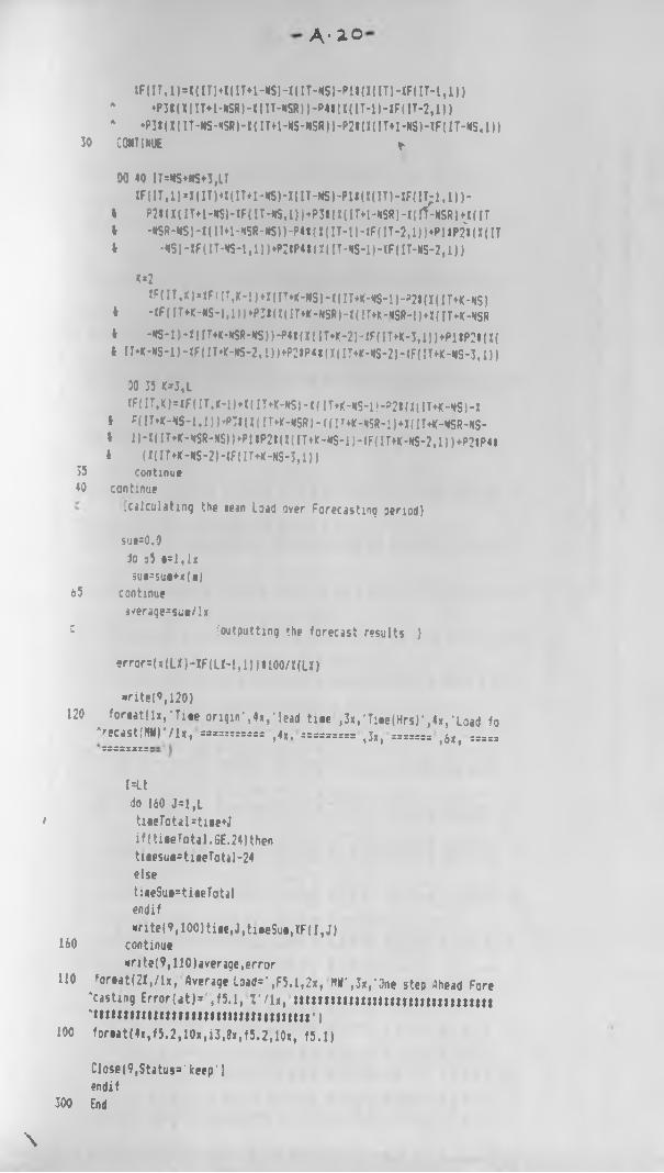
A'20

IF(IT,1)=X(IT|vI(IM-NS)-X(IT-NS)-P1I(I( IT)-XF( IT-1,1))A ♦P3l(l(ITtl-hSR)-I(IT-NSR))-P4IU{IT-l)-XF(IT-2,l))A *P3»( I (IT-MS-*<SR)-X( IT*l-NS-NSR))-P2l(I(IT*l-NS)-XF( IT-MS,l|)

30 CONTINUE *

DO 40 IT*NS»NS*3,LTIFUT,n»I(IT)4l(IT*l-NS)-I(IT-NS)-Pll(I(lTHF(IT;l,l))-

4 P2m(ITtl-N5)-IF(IT-NS,l)|^JI(I(IM-NSR)-l(rT-NSRl4l(IT 4 -«S«-NS)-I(IUl-NSR-NS))-P4t(X(IMHF(IT-2,l))4PllP2'l(l(IT 4 -«S)-IF(tT-NS-l,l)|*:iP4m|IT-NS-lHF(IT-NS-2,i))

4*2IF(IT,K)*!F(|TtK-l)4l(IT44-NS)-l(IT4KHIS-l)-P2t(X(IT4K'NS)

4 -»F(IT«!-NS-l,l))*P3m(IT*K-NSR)-I(IT4K-NSR-!)*]|(IT»IMSR 4 -NS-l)-T(IT*4-NSR-NS))-P4»(||IM(-2HF(IT+K-J,l))*PllP2ta(4 IT»4-NS-l)-(F(IT*r-NS-2,l))4P2IP4l!l(IT4lf-NS-2)-«F(IT44-NS-3ll))30 35 4*3, LfF(IT,4)=lF(IT,4-l)»X(IT»4-hS)-f( IT+4-NS-l!-s2l(X(IT4l(-9S!-l

I F(IM-NS-1,1))*P5I(I(ITHMISR)-»([T44-NSR-1)+I(IT4)HISR-NS- 4 l)-l(IT*K-NSR-NS))4PllP2t(I(ITt4-NS-l)-IF(IT+4-NS-2,l))4P2IP4l 4 (KIT*4-NS-2HF(lT*4-NS-3,i))

35 continue40 continue

.calculating the lean Load over Forecasting period}sue=0.3 do o5 i=l,U 5ue=su#+x(ej

65 continueaverage=sue/lx

: (outputting the forecast results )error=(x(LX)-XF(LI-l,l))I100/I(LX)

120*rite(P,120)

foreatllx,'T:»e origin',4x,‘lead tiee ,3x,'Tiee(Hrs)’,4x,'Load fo Vecast!NN)'/lx, =========== ,4x.========= ,3x,=======f6x, =====

I*Ltdo 160 J=1,L

i tieeTotal=tiee+Jif(ti»eTotal.SE.24)thentuesue=tieeTotaI-24elsetueSu«=ti*eTotalendif»rite(9,100)ti«e,J,tieeSue,TF(I,J)

160 continue«n te(9,110 Javerage, error

110 foreat(2X,/lx, Overage Load*',F5.1,2x, NN',3x,'0ne step Ahead Fore"casting Error(at)* ,f5.1, Z71x, tmumtltltlttltlttltmtltltt'tttmttttiitttmttttitmttmuit')

100 foreat(4x,f5.2,l0x,i3,8x,f5.2,10x, f5.1)

Close(9,Status*'keep') endif

300 End

\

Table 8

P 1W C K W T A C E FC O C TS O F T H * j * D O TT O B irn O S I j C H I s

T ib i * of x * o ; - «>• ' W o p * rc *n ta *e point of th* ,» dtatrtbution fo r » <vt r » i <rf fr**<V>m

S..f> * 995 99 96 975 93 90 80 75 70 50 30 25 20 10 v r 075- 02 01 005 001 - a

w * 1 0*393 0 ’ 157 0 ’ 62S 07962 00393 0156 0647 102 148 *55 i 07* i 323 1 642 2 706 3 8*1 5 024 3 412 6 • 35 7 079 10 0270404 0306 103 211 440 375 713 1 366 2 406 2 773 3 219 4 605 3 991 7 378 7 024 - 9 '210 10 5*7 13 615 i165 216 352 564 1 003 1 213 1 424 2 386 3 865 4 108 4 642 • 251 2 815 9 3*6 • 637 I I 3*5 12 838 10 260 9429 464 711 1 064 1 640 1 923 2 195 1 357 4 878 5 385 5 989 7 779 9 460 n 143 I I . 060 13 277 14 840 10 465 4752 • 31 1 145 1 610 7 343 2 075 3 000 4 351 0 064 • 626 7 269 9 236 11 070/ 12 032 13 368 15 066 16 750 20 317 3e .676> - 672 1 134 1 237 1 635 2 204 3 070 3 433 3 620 5 340 7 331 7 641 0 550 10 645 12 592 14 449 i s 033 16 612 18* 540 22 457 •1 239 1 564 1 690 2 167 * 033 3 622 4 235 4 07 | 6 346 0 363 9 037 9 803 12 017 14 067 16 013 16 622 16 475 20 2TB 24 322 71 344 1 646 2 032 2 160 2 733 O s 490 4 594 5 071 3 527 7 344 9 52* 10 219 11 030 13 362 15 507 17 535 18 168 20 090 21 935 26 125 •1 735 2 066 2 532 2 7 0 0 / ’ 3 325 4 166 3 380 5 699 0 393 6 343 10 636 11 309 12 242 14 084 16 919 19 07 L** 19 679 21 866 23 589 27 077 92 156 2 556 3 059 3 247 3 940 4 665 6 170 6 737 7 26 7 9 342 11 781 12 549 13 442 IS 967 18 307 20 483 21 161 23 209 25 188 29 500 10

i i 2 603 3 053 3 609 3 616 4 573 5 570 6 999 7 584 8 148 10 341 12 699 13 701 14 631 17 275 19 675 21 920 22 610 24 725 28 757 31 264 113 571 4 176 4 404 3 226 6 304 7 007 0 430 9 034 11 340 14 O il 14 845 15 812 18 549 21 026 23 337 24 054 26 217 20 300 32 909 123 56 5 4 107 4 765 5 009 5 892 7 042 6 634 9 299 9 9?0 12 340 15 119 15 904 16 905 19 012 22 .762 24 736 25 472 27 680 29 819 34 520 1314 4 075 4 660 5 366 5 629 0 571 7 790 9 467 10 163 10 • 21 13 339 16 222 17 117 18 151 21 064 23 685 26 119 26 073 29 141 31 319 36 123 144 601 3 229 5 963 6 262 7 261 6 547 10 307 n 036 i i 721 14 339 17 322 19 2*5 19 311 22 307 24 996 27 400 16 259 so 371 32 601 37 697 ISIS 5 142 3 612 6 614 6 908 7 962 9 312 n 152 i i 912 12 624 IS . 336 IB *18 19 369 20 485 23 542 26 296 28 9*3 29 833 32 000 34 267 39 252 1017 5 697 6 406 7 255 7 564 6 672 10 065 12 002 12 792 13 531 16 338 19 511 20 469 21 615 24 769 27 587 30 191 30 995 3.7 409 35 710 40 790 1716 6 265 7 013 7 906 6 231 9 390 10 665 12 857 13 673 14 440 17 338 20 001 21 605 22 700 25 969 26 669 31 526 32 346 34 005 37 156 42 712 IS16 6 644 7 *633 6 567 6 907 10 117 11 651 13 716 14 562 15 352 36 338 21 689 22 719 23 900 27 204 30 144 32 052 33 687 36 191 30 582 43 820 197 434 6 ,260 9 237 9 591 10 631 12 443 14 U 6 15 *52 16 260 19 337 22 775 23 826 25 036 26 412 31 410 34 170 35 020 37 566 39 987 43 313 2021 6 034 6 697 9 913 10 263 11 591 13 240 15 443 16 344 17 187 20 337 23 030 2* 935 20 171 29 615 32 671 35 470 36 343 38 932 41 401 46 797 2122 1) 643 9 542 10 600 10 982 12 336 14 041 16 314 17 740 10 101 21 337 24 939 26 039 27 301 30 613 33 924 36 781 37 659 40 269 42 796 40 260 2223 9 260 10 196 11 293 11 666 13 091 14 040 17 107 10 137 10 071 22 337 20 018 27 141 20 429 32 007 35 172 3f 070 30 960 41 636 44 181 49 720 2324 • 666 10 656 11 9U2 12 401 13 646 15 659 10 062 19 0?7 19 943 23 337 27 096 26 241 29 553 33 196 36 415 39 364 40 270 42 960 45 530 51 179 2425 10 320 11 524 12 697 13 120 14 611 16 473 I I 940 19 939 20 667 24 337 26 172 29 339 30 675 34 382 37 652 40 640 41 568 44 314 40 •26 32 620 3326 11 160 12 196 13 409 13 644 15 379 17 292 19 820 20 643 21 792 336 29 246 30 *3* 51 793 35 563 30 685 41 923 62 156 45 6*2 48 290 5* 052 2627 m o ? 12 679 14 125 14 573 16 151 16 114 20 703 21 7*9 22 719 26 336 30 319 31 528 32 912 36 7*1 *0 113 *3 19* 44 1*0 *6 96 3 *9 6*5 S3 *76 2726 12 461 13 365 14 64 7 15 306 16 928 16 939 21 368 22 857 23 6*7 27 336 31 391 32 620 34 027 37 916 41 337 44 461 *5 419 46 270 50 993 56 693 7029 IS 121 14 236 15 574 16 047 17 708 19 700 22 475 23 567 24 577 26 330 32 401 S3 711 35 139 39 007 *2 557 45 722 46 693 49 508 52 336 50 302 7913 7 67 14 953 16 306 I f 791 10 493. 70 509 23 364 24 476 25 500 20 338 33 530 34 600 30 250 40 256 43 773 46 • 79 47 962 50 692 53 072 59 703 3040 20 706 2? 164 23 630 24 433 20 509 79 051 32 343 33 660 34 677 30 335 44 105 45 610 47 269 51 005 55 759 39 342 00 436 63 691 60 760 73 402 4050 27 991 29 707 31 664 32 357 34 704 37 609 41 449 42 942 44 313 49 333 54 723 56 334 50 164 03 167 67 305 71 420 72 613 70 154 70 460 86 661 5060 35 535 37 465 39 699 40 402 43 166 46 439 50 641 32 204 53 009 59 333 65 227 66 901 66 972 7* 397 79 002 03 296 64 500 08 379 91 932 99 607 6070 43 273 43 442 47 693 46 750 31 739 55 379 39 896 61 699 63 346 wo 334 75 669 77 577 79 715 85 527 90 531 95 023 96 308 100 425 104 215 112 317 70S I 171 53 539 56 213 57 153 60 391 64 270 60 207 71 143 72 013 70 334 •6 120 66 130 90 405 96 578 101 MO 106 679 100 069 112 .729 l i e 321 124 039 BO90 59 196 61 754 64 634 63 646 69 126 73 291 70 330 00 623 • 7 311 00 334 06 524 98 •30 101 054 107 565 113 145 110 136 119 640 124 116 126 299 137 200 9 0100 67 327 70 065 73 142 74 222 77 929 67 330 67 043 00 133 07 129 90 334 106 900 109 141 111 667 110 490 ■ 24 342 129 561 131 1*2 133 807 140 170 149 449 100

F o r v a l u t a of v > 30 approxim ate va lu ta fo r may be obtained from tht tx p rta a lo n *•‘ 9 - •V c \ '» i ]■ « h * r * ?n la th t norm al d tv U t t cu tt ln f off tht co rrvapondtnc ta ll a of a norm al d latrlbutlon

U ? U taken i t the 0 0? I a v a l, io that 0 01 o( the norm al d istrib u tio n la In ta c h ta ll , th* *xp r*a a ln n y ie ld * ■f a l th» 0 99 and 0 01 point* F o r t * ry l a r j * va lu es o l y it la m f f lc lrn t ly accu ra l# to rompuW

• 7 ? th* d la lr lb u t in n of a h lr h la ap proa lm ale ly norm al around a mean ol .'2# - I and with a standard deviation ot 1 TW a u b l* la taken by consent from S ta t is t ic a l Tab le* for p io ln c lc a l A * r (cu ltu ra l,and M ed ica l R * a * a rc h , b> R A F ia h e i and f Vatea, published by O liv e r and Boyd. Cd lnhu rfh . and from Table I of R lo m etrfka Tahlea for S ta f la t ir la n a . Vol I . h> perm laa lon of the R inm etrU t* T roeieee