On Short-Term Load Forecasting Using Machine Learning ...

HAL Id: hal-03187029https://hal.archives-ouvertes.fr/hal-03187029

Submitted on 31 Mar 2021

HAL is a multi-disciplinary open accessarchive for the deposit and dissemination of sci-entific research documents, whether they are pub-lished or not. The documents may come fromteaching and research institutions in France orabroad, or from public or private research centers.

L’archive ouverte pluridisciplinaire HAL, estdestinée au dépôt et à la diffusion de documentsscientifiques de niveau recherche, publiés ou non,émanant des établissements d’enseignement et derecherche français ou étrangers, des laboratoirespublics ou privés.

On Short-Term Load Forecasting Using MachineLearning Techniques and a Novel Parallel Deep

LSTM-CNN ApproachBehnam Farsi, Manar Amayri, Nizar Bouguila, Ursula Eicker

To cite this version:Behnam Farsi, Manar Amayri, Nizar Bouguila, Ursula Eicker. On Short-Term Load Forecasting UsingMachine Learning Techniques and a Novel Parallel Deep LSTM-CNN Approach. IEEE Access, IEEE,2021, 9, pp.31191 - 31212. �10.1109/access.2021.3060290�. �hal-03187029�

https://hal.archives-ouvertes.fr/hal-03187029

https://hal.archives-ouvertes.fr

Received February 7, 2021, accepted February 15, 2021, date of publication February 18, 2021, date of current version March 1, 2021.

Digital Object Identifier 10.1109/ACCESS.2021.3060290

On Short-Term Load Forecasting UsingMachine Learning Techniques and a NovelParallel Deep LSTM-CNN ApproachBEHNAM FARSI 1, MANAR AMAYRI2, NIZAR BOUGUILA 1, (Senior Member, IEEE),AND URSULA EICKER31Concordia Institute for Information Systems Engineering(CIISE), Concordia University, Montreal, QC H3G 1M8, Canada2G-SCOP Lab, Grenoble Institute of Technology, 38185 Grenoble, France3Department of Building, Civil and Environmental Engineering, Concordia University, Montreal, QC H3G 1M8, Canada

Corresponding author: Behnam Farsi ([email protected])

ABSTRACT Since electricity plays a crucial role in countries’ industrial infrastructures, power companiesare trying to monitor and control infrastructures to improve energy management and scheduling. Accurateforecasting is a critical task for a stable and efficient energy supply, where load and supply are matched. Thisarticle discusses various algorithms and a new hybrid deep learning model which combines long short-termmemory networks (LSTM) and convolutional neural network (CNN) model to analyze their performancefor short-term load forecasting. The proposed model is called parallel LSTM-CNN Network or PLCNet.Two real-world data sets, namely ‘‘hourly load consumption of Malaysia ’’ as well as ‘‘daily power electricconsumption of Germany’’, are used to test and compare the presentedmodels. To evaluate the testedmodels’performance, root mean squared error (RMSE), mean absolute percentage error (MAPE), and R-squaredwere used. In total, this article is divided into two parts. In the first part, different machine learning models,including the PLCNet, predict the next time step load. In the second part, the model’s performance, whichhas shown the most accurate results in the first part, is discussed in different time horizons. The results showthat deep neural networks models, especially PLCNet, are good candidates for being used as short-termprediction tools. PLCNet improved the accuracy from 83.17% to 91.18% for the German data and achieved98.23% accuracy in Malaysian data, which is an excellent result in load forecasting.

INDEX TERMS Electricity, smart grids, load consumption, short-term load forecasting, deep learning, timeseries, regression, convolutional neural networks, long short-term memory.

NOMENCLATUREANN : Artificial Neural NetworkARIMA : Autoregressive Integrated Moving AverageCNN : Convolutional Neural NetworkDNN : Deep Neural NetworkETS : Exponential SmoothingLSTM Long Shot-Term MemoryLTLF : Long-Term load forecastingMLR : Multiple Linear RegressionMTLF : Medium-Term Load ForecastingRNN : Recurrent Neural NetworkSARIMA : Seasonal ARIMASTLF : Short-Term Load ForecastingSVR : Support Vector Machine

The associate editor coordinating the review of this manuscript and

approving it for publication was Li Zhang .

I. INTRODUCTIONAccording to the IEA report [1], in 2017, world electricityconsumption reached 21,372 TWh, which is 2.6% higher than2016 electricity consumption. Such an annual increase cre-ates a new problem: how to reduce consumption? Nowadays,many companies are working on this problem and trying tosolve it. Demand Response Management, which is one of themain features in smart grids [2], helps to control electricityconsumption with the focus on the customer side. It is alsomore essential to understand residential and non-residentialbuilding demand and the use of electricity. Carrying out areduction in load consumption can lead to a high number ofeconomic and environmental benefits. Since experts aim tocreate some automated tools that are able to deliver energyvery efficiently, they introduced load forecasting methodsas alternative solutions for electricity network augmentationas it can be useful to manage the electricity demand and

VOLUME 9, 2021 This work is licensed under a Creative Commons Attribution 4.0 License. For more information, see https://creativecommons.org/licenses/by/4.0/ 31191

https://orcid.org/0000-0002-7287-2989

https://orcid.org/0000-0001-7224-7940

https://orcid.org/0000-0001-6674-692X

B. Farsi et al.: On Short-Term Load Forecasting Using Machine Learning Techniques and a Novel Parallel Deep LSTM-CNN Approach

provide more energy efficiency [3]. In addition, improvingpower delivery quality and having secure networks is a crit-ical task in smart grids to monitor and support advancedpower distribution systems [4] and, in particular, to improveload forecasting. Since future consumption could be pre-dicted, they can be considered as tools to minimize the gapbetween electricity supply and user consumption. However,an inaccurate prediction may lead to a huge loss. For instance,a small percentage of increase in forecast error was predictedin 1985, which led to more than 10 million pounds of yearlydetriment in the thermal UK power systems [5]. Thus, manybig companies have focused on accurate load forecasting andload management so that the Energy Supply Association ofAustralia, as an instance, invested about 80% of its budget ongrid upgrades.

Load forecasting approaches are categorized in three dif-ferent groups concerning their functionalities for differ-ent purposes [7]: Short-term Load Forecasting (STLF) [8],Medium-term Load Forecasting (MTLF) and Long-termLoad Forecasting (LTLF) [9]. STLF forecasts the followinghour load to next week, while in MTLF, it is more than oneweek to few months, and LTLF forecasts next years loadconsumption. For each of these methods, there are diversefactors that influence the prediction.

Due to the ability of STLF approaches, they have tremen-dous importance in energy management. Hence, they havebeen used to provide proper management in electric equip-ment, and because of this contribution, they are known asan inevitable component in Energy Management Systems.An error in STLF can have an immediate impact on electricalequipment. Several factors affect the STLF, including thefollowing ones: (1) Time factor [6], which is the most crucialfactor for STLF because of the existence of some patternssuch as daily patterns in a set of data (2) Climate, which con-tains temperature and humidity [6]. (3) Holidays can makeconsiderable changes in electricity demand. However, thisarticle focuses on time as a factor that influences electricityusage and can help achieve accurate predictions.

Besides, diverse approaches can be applied to time-seriesdata to carry out accurate short-term forecasting. Theseapproaches consist of statistical regression models, classictime-series models, and deep learning models. However,in addition to the factors as mentioned earlier, there are otherfactors such as the size of the house, the age of appliancesand equipment [6], global factors like diseases, which canaffect the load prediction for medium-term and long-termforecasting. Still, most approaches have the same attributeswith some subtle differences. Load consumption data sets canbe viewed as time series. time-series have specific attributes,such as Trend, Seasonality, and Noise, which will be dis-cussed later. Due to numerous challenging problems whendealing with time-series data, researchers deployed ArtificialNeural Networks (ANN) [18] which have structures likethe human brain. They are available to be used in variousareas such as Natural Language Processing (NLP) [10], audiorecognition [11], medical [12] and load forecasting [19] and

they have been successful to achieve impressive results. Oneof the challenging problems of ANN is that they need largescale data for training to learn the models. Therefore, in somecases, regression-based approaches can be more useful.

Different algorithms for load forecasting have been studiedso far. The authors in [6] prepared an overview of differenttypes of load forecastingmethods. They focused on the differ-ence between short-term, medium-term, and long-term loadforecasting and the factors which affect them. The authors in[14] discussed a review of load forecasting with a focus onregression-based approaches. To forecast day-ahead hourlyelectricity load, they used two particular data sets from theUniversity of New South Wales, one from the Kensing-ton Campus and the Tyree Energy Technologies Building.The authors in [7] surveyed different deep learning mod-els for short-term load forecasting. They evaluated sevendeep learning models on three real-world data sets. Theyproved that there is no correlation between the complexityof models and golden results. Even in some cases, simplermodels can achieve better results in short-term load fore-casting. The authors in [15] proposed a hybrid deep neuralnetwork consisting of a CNNmodule, an LSTMmodule, anda feature-fusion module and tested it on the 2-year electricload data sets from the Italy-North area. Their model wascompared with some other machine learning models, includ-ing: Decision Tree, Random Forest, DeepEnergy, LSTM, andCNN coming with better results. However, even though theyachieved good results from their proposed model, their useddata set was not challenging. The authors did not challengethe model with a more complex data set or prediction indifferent time horizons. The author in [16] proposed a parallelCNN-RNN model to predict one day ahead of load con-sumption. Temperatures, holidays, hours of day, and days ofthe week were used as features for the historical load seriesand achieved better results than regression-based models,DNN and CNN-RNN. However, due to the existing vanishinggradient descent problem in RNNs, they are not suitableenough to be used in load forecasting applications, and LSTMnetworks should replace them. RNNs and the specific typeof their family, LSTM, use control theory in their structure.They can find the dependency between old data and newones and become an interesting network for load forecastingapplications in recent years. [17] has studied RNNs modelswell. The authors in [20] proposed a new DeepEnergy modelthat combines 1-D CNN to extract the features and fullyconnected network to forecast future load data. To forecastthe next three days’ data, they used an hourly electricityconsumption data set from the USA. They compared the pro-posed model’s result with five other machine learning tech-niques through RMSE and MAPE. The results showed thatthe DeepEnergy model could carry out an accurate short-termload forecasting compared to other models. After the Deep-Energy model, the Random Forest technique [21] had a goodperformance. However, as there is no LSTM network in thismodel, it will have some difficulty working with more com-plex time-series data, and it can be expected that this model

31192 VOLUME 9, 2021


may fail to make an accurate prediction. In another study[23], the authors proposed a new model which consists ofthree algorithms including Variational Mode Decomposition(VMD), Convolutional Neural Network (CNN), and GatedNeural Network (GRU). For more convenience, they calledthe proposed model SEPNet. This model aimed to predicthourly electric price and evaluate the model, hourly data fromcity Newyork, the USA, which includes the hourly electricityprice from 2015 to 2018. Compared to other models suchas LSTM, CNN, VMD-CNN, the SEPNet model performedbetter where it improved the RMSE and MAPE by 25%and 19%, respectively. The existing problem with SEPNetis that CNN and GRU are designed consecutively in thismodel, so the processed data from CNN may affect the GRUnetwork’s performance. Some authors, such as in [24] usedANNs to forecast other types of load data like PV system out-put data. They proposed a powerful CNN based model calledPVPNet, and they evaluated the proposed model by usingdaily data from 2015. They used three past days’ informationto predict the next 24h and their model has outperformedRan-dom Forest (RF) regarding the mean absolute error (MAE)and RMSE. Besides, with technology development, manystudies deployed machine learning models in IoT. In termsof the technical part, if these models are supposed to beused in IoT, they must perform online load forecasting. [27]presents some related machine learning methods which canbe used in IoT through the cloud. They also implementeda novel hardware technology, including the Arduino micro-controller. They implemented the device in a research lab topredict total power consumption in the lab. Regarding thealgorithms, Linear Regression, SVM Regression, EnsembleBagged, Ensemble Boosted, Fine Tree Regression, and Gaus-sian Process Regression (GPR) have been used. All of thementioned models have performed appropriately.

Even though some studies in recent years have discusseddifferent models for short-term load forecasting [22], the lackof a comprehensive article to carry out a comparison betweenclassic time-series models, regression-based models, anddeep learning is completely obvious. Besides, time-seriesmust be used correctly as input for machine learning models.In other words, some analysis of data is essential to com-pile machine learning models. This article ’s contributionis that it focuses on different models that are appropriateto be used for load forecasting, and it also reviews somedifferent methodologies to find out the most effective mod-els for forecasting applications. Even though various deeplearning models have been introduced for load forecastingin recent years, only some have succeeded in achievingstate-of-the-art results. Moreover, this article consecu-tively proposes a new hybrid parallel CNN-LSTM andLSTM-Dense neural networks to improve load forecastingaccuracy. Regarding the model’s architecture, it consists oftwo different paths (CNN and LSTM). CNN path extracts theinput data features, and the LSTM path learns the long-termdependency within input data. After passing through thesetwo paths and merging their outputs, a fully connected path

FIGURE 1. An overview of the article.

combined with an LSTM layer has been implemented to pro-cess the output to predict final load data. This article aims toevaluate various machine learning techniques in STLF taskswhile there are no exogenous variables. In other words, it triesto find out a way to carry out STLF using just previous loaddata and compare all the results with each other. To extend thisstudy, all the models are implemented to forecast daily andhourly ahead load consumption using two highly aggregateddata sets, one of which is an hourly power consumption fromthe city of Johor in Malaysia [25]. The other one is a dailyelectric consumption which is collected from a power supplycompany in Germany. In order to evaluate the models, thisarticle uses root mean squared error (RMSE) due to the abilityto show how much predicted values spread around averageand mean absolute percentage error (MAPE) since MAPEcan present the accuracy of the models and R-Squared toshow the correlation between predicted results and actualvalue.

The remainder of the article is organized as follows:section II discusses how time-series data and associatedmodels work. Section III, in addition to discussing datapre-processing, elaborates the models and show the results.Finally, a conclusion is issued in section IV.

II. BACKGROUND OF STUDYLoad series data usually have particular attributes. Thus,before forecasting future load consumption, these attributesmust be studied and discussed as follows.

A. DEFINITIONSAs it has been mentioned before, load consumption data aretime series. Thus, to forecast future load consumption, sometime-series analyses are needed. time-series have importantattributes such as trend or noise. In order to predict future loadconsumption, some considerations of time-series are neededto be taken into account.

1) TRENDSome time-dependent data have a linear trend in the longterm. It means there is an increase or decrease duringthe whole time, which may not be in the same directionthroughout the given period. However, overall, it will beupward, downward or stable. Load series data are an excellentexample of a kind of tendencies of movement.

VOLUME 9, 2021 31193


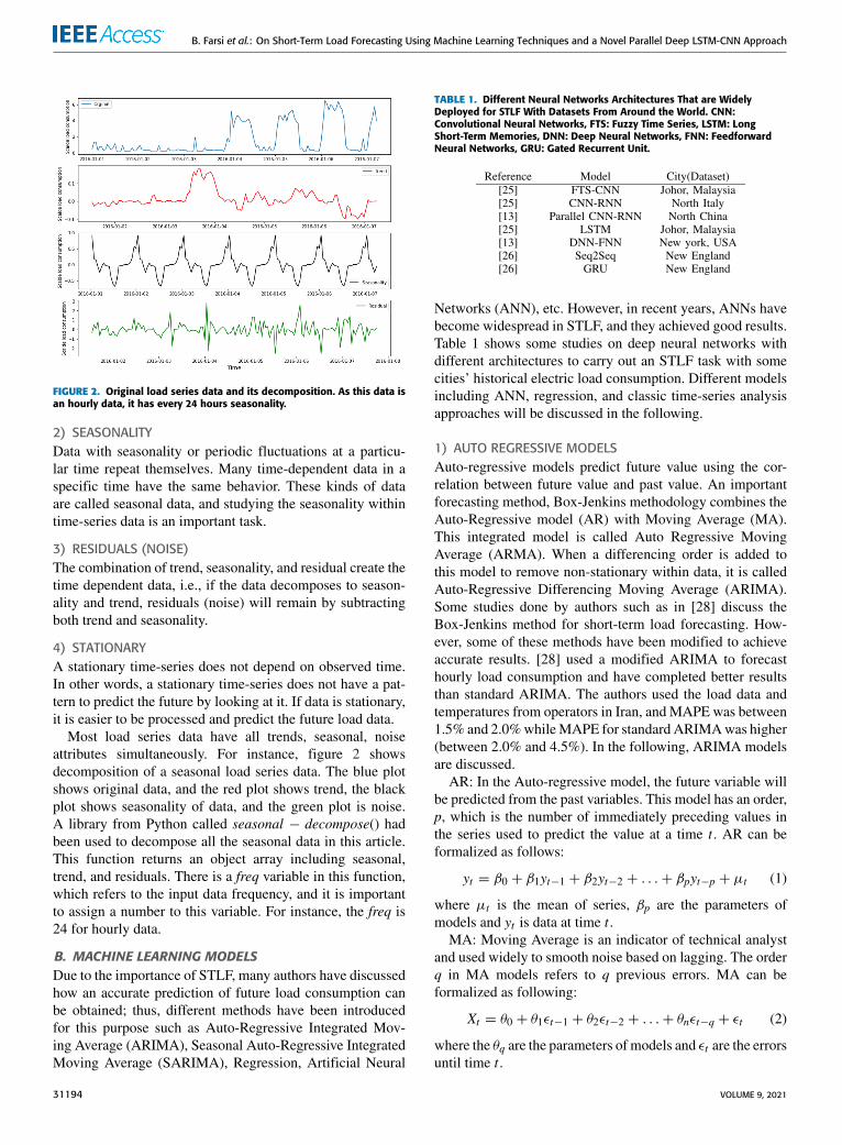
FIGURE 2. Original load series data and its decomposition. As this data isan hourly data, it has every 24 hours seasonality.

2) SEASONALITYData with seasonality or periodic fluctuations at a particu-lar time repeat themselves. Many time-dependent data in aspecific time have the same behavior. These kinds of dataare called seasonal data, and studying the seasonality withintime-series data is an important task.

3) RESIDUALS (NOISE)The combination of trend, seasonality, and residual create thetime dependent data, i.e., if the data decomposes to season-ality and trend, residuals (noise) will remain by subtractingboth trend and seasonality.

4) STATIONARYA stationary time-series does not depend on observed time.In other words, a stationary time-series does not have a pat-tern to predict the future by looking at it. If data is stationary,it is easier to be processed and predict the future load data.

Most load series data have all trends, seasonal, noiseattributes simultaneously. For instance, figure 2 showsdecomposition of a seasonal load series data. The blue plotshows original data, and the red plot shows trend, the blackplot shows seasonality of data, and the green plot is noise.A library from Python called seasonal − decompose() hadbeen used to decompose all the seasonal data in this article.This function returns an object array including seasonal,trend, and residuals. There is a freq variable in this function,which refers to the input data frequency, and it is importantto assign a number to this variable. For instance, the freq is24 for hourly data.

B. MACHINE LEARNING MODELSDue to the importance of STLF, many authors have discussedhow an accurate prediction of future load consumption canbe obtained; thus, different methods have been introducedfor this purpose such as Auto-Regressive Integrated Mov-ing Average (ARIMA), Seasonal Auto-Regressive IntegratedMoving Average (SARIMA), Regression, Artificial Neural

TABLE 1. Different Neural Networks Architectures That are WidelyDeployed for STLF With Datasets From Around the World. CNN:Convolutional Neural Networks, FTS: Fuzzy Time Series, LSTM: LongShort-Term Memories, DNN: Deep Neural Networks, FNN: FeedforwardNeural Networks, GRU: Gated Recurrent Unit.

Networks (ANN), etc. However, in recent years, ANNs havebecome widespread in STLF, and they achieved good results.Table 1 shows some studies on deep neural networks withdifferent architectures to carry out an STLF task with somecities’ historical electric load consumption. Different modelsincluding ANN, regression, and classic time-series analysisapproaches will be discussed in the following.

1) AUTO REGRESSIVE MODELSAuto-regressive models predict future value using the cor-relation between future value and past value. An importantforecasting method, Box-Jenkins methodology combines theAuto-Regressive model (AR) with Moving Average (MA).This integrated model is called Auto Regressive MovingAverage (ARMA). When a differencing order is added tothis model to remove non-stationary within data, it is calledAuto-Regressive Differencing Moving Average (ARIMA).Some studies done by authors such as in [28] discuss theBox-Jenkins method for short-term load forecasting. How-ever, some of these methods have been modified to achieveaccurate results. [28] used a modified ARIMA to forecasthourly load consumption and have completed better resultsthan standard ARIMA. The authors used the load data andtemperatures from operators in Iran, and MAPE was between1.5% and 2.0%whileMAPE for standard ARIMAwas higher(between 2.0% and 4.5%). In the following, ARIMA modelsare discussed.

AR: In the Auto-regressive model, the future variable willbe predicted from the past variables. This model has an order,p, which is the number of immediately preceding values inthe series used to predict the value at a time t . AR can beformalized as follows:

yt = β0 + β1yt−1 + β2yt−2 + . . .+ βpyt−p + µt (1)

where µt is the mean of series, βp are the parameters ofmodels and yt is data at time t .MA: Moving Average is an indicator of technical analyst

and used widely to smooth noise based on lagging. The orderq in MA models refers to q previous errors. MA can beformalized as following:

Xt = θ0 + θ1εt−1 + θ2εt−2 + . . .+ θnεt−q + εt (2)

where the θq are the parameters of models and εt are the errorsuntil time t .

31194 VOLUME 9, 2021


FIGURE 3. ACF plot for an example data. X axis shows number of lags,Y axis shows amount of auto-correlation.

Integration: To predict future load consumption withARIMA model, a stationary time-series should be used.There are different methods to stabilize a time series, such aslogarithm or differencing. These operators reduce time-serieschanges with trend elimination; in other words, they convertnon-stationary data to stationary data. An ARIMA modelusually is written as ARIMA(P,D,Q) to show the neededorders, which should be used to achieve the best results fromthismodel.D represents the number of integration used,P andQ represent the orders of AR andMA part of ARIMA. To findout the values of P, D, and Q, there are different approaches.However, many experts suggest using auto-correlation (AC)and Partial auto-correlation (PAC) plots to figure out thevalues of P and Q. Nevertheless, first of all, it is necessaryto find out what AC is precise. AC is the degree of similaritybetween a time-series data and its lags (see figure 3), and ittakes a value in the range [−1,1]. If there is any seasonalityin data, remarkable spikes in the AC plot are shown. Forinstance, figure 3 shows theAC plot (or auto-correlation func-tion (ACF) plot) of an hourly load consumption from a smartbuilding in France. This data is an hourly load consumptiondata, and because of this hourly attribute, a seasonal approachevery 24 hours can be seen in this figure.

Likewise, P or, in other words, the order of AR which isa part of ARIMA model can be found by plotting PAC plot(or partial auto-correlation function (PACF) plot). Figure 4shows the PAC plot for same data in figure 3.However, there are some other tests to find the best values

for D. To figure out whether the data is stationary or not,two different tests are proposed: The rolling statistic plot testand the Dickey-Fuller test. The rolling statistic plot test is achart analysis technique to examine collected data by plottingRolling Average. Figuring out the existence of a trend in theRolling average is the primary objective. Provided there isnot any trend, data is determined as stationary. In figure 5,the blue plot shows the original data, and the red plot showsthe rolling average of data. Since there is no trend in the

FIGURE 4. PACF plot for same data in figure 3.

FIGURE 5. An example of Rolling test which proves that data is stationary.

rolling average plot (red plot), the data is stationary. Besides,a Dickey-Fuller test has been applied to this data. This testis based on a null hypothesis in which the nature of theseries (i.e., stationary or not) could be determined by eval-uating the p-value received by the Dickey-Fuller test. Thep-value is considered as a critical value for rejecting the nullhypothesis. Thus, the smaller p-value provides more robustevidence to accept the alternative hypothesis. In this example,the confidence interval is supposed 5%, and after applying thetest, the obtained p-values are less than 0.05, so data can beconsidered stationary.

Hence, one way to obtain the best values for D, after anyintegration of data, Rolling tests and Dickey-Fuller test canbe applied. If these tests prove data is stationary, there is noneed to carry out another integration. However, in case theresults were different, it demonstrates that data need moreintegration. It must be said that in some instances achievingstationary data is not possible. Therefore, this type of datacannot work with ARIMA models.

VOLUME 9, 2021 31195


Seasonal ARIMA or SARIMA is another kind of statisticalmodel that is widely used in seasonal data cases. In addition tothe same parameters with ARIMA (P,D,Q)) four other param-eters for the seasonal part of these models are p, d , q and m.Like ARIMA, p represents the order of Auto-regressive forthe seasonal part, d represents the order of integration for theseasonal part, and q represents the order of Moving Averagefor the seasonal part. Besides, m shows the time horizon ofseasonality. For example, for hourly data, m will be 24, andfor daily data, it will be 7. Therefore, SARIMA formulationis usually presented as SARIMA (P,D,Q)(p,d,q,m).

2) EXPONENTIAL SMOOTHINGExponential Smoothing (ETS) is a well-known time-seriesforecasting model for power systems. It can be used as analternative to ARIMA models, in addition to its ability tobe used for STLF, MTLF, and LTLF. It uses a weightedsum of past observations to make the prediction. The dif-ference between ETS and ARIMA models is that ETS usesan exponential decreasing weight for previous observations.It means recent observations have a higher weight than pastobservations. Therefore the accuracy depends on some coef-ficients. The authors in [29] studied exponential smoothingfor load forecasting application using different coefficients.They used six different data sets collected from China toevaluate their model, and as it was assumed, they achieved ahigh range of MAPE for different coefficient values. Thereare various types of ETS models that are used due to thecomplexity of data. Equation (3) indicates the formula of thesimple Exponential Smoothing

Ft+1 = αAt + (1− α)Ft (3)

where Ft and Ft+1 indicate, predicted value in time t and t+1respectively, At indicates actual value at time t and α is thesmoothing factor (0 ≤ α ≤ 1).

3) LINEAR REGRESSIONRegression-based approaches are interesting techniques,and among all these techniques, linear regression has aninevitable role. Some studies tried to use linear regression fortime-series or specifically for load forecasting. The authorin [30] studied RGUKT, R.K valley campus for STLF andachieved MAPE = 0.029 and RMSE = 2.453. In anotherstudy, the authors in [31] used it with different linear regres-sion models, including multiple linear regression (MLR),Lasso, Ridge for hourly load data.

Linear regression is a statistical method to find the relationamong variables. This method is useful to estimate a variableusing influence parameters. The most straightforward linearregression equation is as below:

Yi = β0 + β1Xi + µi (4)

where Y is the dependent variable, β0 is an interceptor, β1 isthe slope, X is the independent variable, and µi is residual ofthe model, which is distributed with zero mean and constantvariance. By increasing the number of variables, this model

is called multiple linear regression (MLR). In order to eval-uate this model, the Least Squared Error (LSE) technique isused. The primary goal is that to find the best coefficients tominimize LSE. LSE evaluates the model by adding squaresof error between two variables, which in this case, is betweenactual values and forecasted ones. Equation (5) shows LSEformula:

LSE =n∑i=1

(Yi − Xi)2 (5)

where X is predicted value, Y is the actual value.In order to use linear regression for load forecasting, some

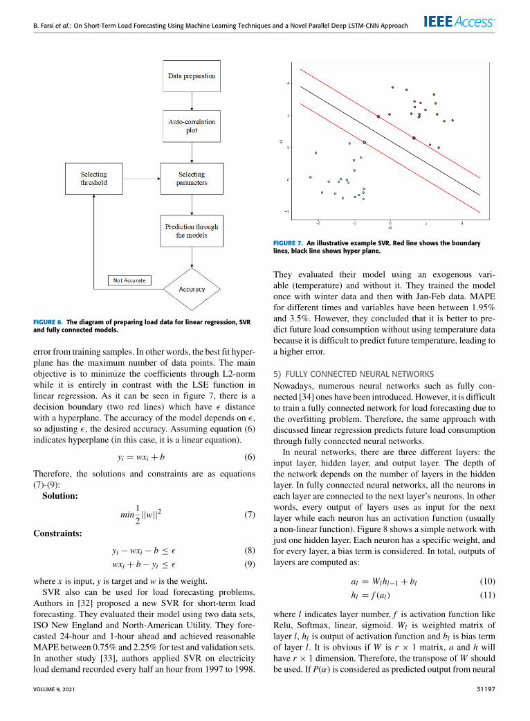
parameters such as temperature, humidity, time are neededto be used as independent variables. Likewise, the loadconsumption data are used as dependent variables in lin-ear regression models. With this approach, it is possible touse linear regression to forecast future load consumption.However, there are some ways to forecast load consumptionwithout using exogenous variables. Lags can be used as theindependent variable for load forecasting to predict linearregression without using exogenous data. Usually, more thanone lag is used as an independent variable, so MLR is usedinstead of simple linear regression. AC plot is a useful tool fortime-series analysis with linear regression. In this approach,those lags inwhich their auto-correlation values aremore thana certain threshold can be used as an independent variablein linear regression. For instance, according to figure 3 lags[1, 2, 3, 24, 25] are chosen as independent variables withamount 0.6 for threshold. In total, in this model, lags are inde-pendent variables, and actual load consumption is the depen-dent variable. An alternative way to increase the model’saccuracy is that exogenous variables such as humidity, hol-iday, and weather are added to the model. Figure 6 shows theprocess of preparing data and choosing parameters for linearregression models. This approach also is used for SVR andfully connected models too. According to the diagram, datapreparation refers to finding missing values and data normal-ization. As discussed after plotting the AC plot, those lagswith higher auto-correlation value than the selected thresholdare used as the models’ parameters. After choosing lags andparameters, the models can predict again, however, if theyare not accurate enough, the amount of the threshold must bechanged, and the process is also re-started.

4) SUPPORT VECTOR REGRESSION (SVR)Support vector machine (SVM) is an approach that is usedfor classification and regression problems. SVM has becomean exciting model among machine learning techniques due tothis model’s ability in different issues such as text or imageanalysis. For instance, the authors in [14] studied SVM forsupervised learning methods. However, the first objective ofSVM was classification. Nonetheless, this model has beenextended to regression problems after a while, called supportvector regression (SVR). SVR has the same procedure asSVM,with some differences. This model’s objective is to findthe most appropriate hyperplane with minimum acceptable

31196 VOLUME 9, 2021


FIGURE 6. The diagram of preparing load data for linear regression, SVRand fully connected models.

error from training samples. In other words, the best fit hyper-plane has the maximum number of data points. The mainobjective is to minimize the coefficients through L2-normwhile it is entirely in contrast with the LSE function inlinear regression. As it can be seen in figure 7, there is adecision boundary (two red lines) which have ε distancewith a hyperplane. The accuracy of the model depends on ε,so adjusting ε, the desired accuracy. Assuming equation (6)indicates hyperplane (in this case, it is a linear equation).

yi = wxi + b (6)

Therefore, the solutions and constraints are as equations(7)-(9):

Solution:

min12||w||2 (7)

Constraints:

yi − wxi − b ≤ ε (8)

wxi + b− yi ≤ ε (9)

where x is input, y is target and w is the weight.SVR also can be used for load forecasting problems.

Authors in [32] proposed a new SVR for short-term loadforecasting. They evaluated their model using two data sets,ISO New England and North-American Utility. They fore-casted 24-hour and 1-hour ahead and achieved reasonableMAPE between 0.75% and 2.25% for test and validation sets.In another study [33], authors applied SVR on electricityload demand recorded every half an hour from 1997 to 1998.

FIGURE 7. An illustrative example SVR. Red line shows the boundarylines, black line shows hyper plane.

They evaluated their model using an exogenous vari-able (temperature) and without it. They trained the modelonce with winter data and then with Jan-Feb data. MAPEfor different times and variables have been between 1.95%and 3.5%. However, they concluded that it is better to pre-dict future load consumption without using temperature databecause it is difficult to predict future temperature, leading toa higher error.

5) FULLY CONNECTED NEURAL NETWORKSNowadays, numerous neural networks such as fully con-nected [34] ones have been introduced. However, it is difficultto train a fully connected network for load forecasting due tothe overfitting problem. Therefore, the same approach withdiscussed linear regression predicts future load consumptionthrough fully connected neural networks.

In neural networks, there are three different layers: theinput layer, hidden layer, and output layer. The depth ofthe network depends on the number of layers in the hiddenlayer. In fully connected neural networks, all the neurons ineach layer are connected to the next layer’s neurons. In otherwords, every output of layers uses as input for the nextlayer while each neuron has an activation function (usuallya non-linear function). Figure 8 shows a simple network withjust one hidden layer. Each neuron has a specific weight, andfor every layer, a bias term is considered. In total, outputs oflayers are computed as:

al = Wlhl−1 + bl (10)

hl = f (al) (11)

where l indicates layer number, f is activation function likeRelu, Softmax, linear, sigmoid. Wl is weighted matrix oflayer l, hl is output of activation function and bl is bias termof layer l. It is obvious if W is r × 1 matrix, a and h willhave r × 1 dimension. Therefore, the transpose of W shouldbe used. If P(α) is considered as predicted output from neural

VOLUME 9, 2021 31197


FIGURE 8. A one-layer neural network example.

networks, α represents parameters of neural network and y isthe actual value, for N input-output, the loss function is:

L =1N6Ni=1(yi − P(α))

2 (12)

The primary goal is to optimize the parameters of theneural network. For the same purpose, the loss functionmust be minimized as much as possible. A regularizationpenalty term is usually used to avoid overfitting (see equation(13)). Overfitting refers to the production of analysis froma statistical model that is extremely trained. The problem isthat when overfitting happens, the model learns very wellthe parameters but it is not able to predict well (i.e. weakgeneralization ability) [35].

L =1N6Ni=1(yi − P(α))

2+�(α) (13)

where �(α) = λ||α||2, using norm-2 and a hyperparameterto control the regularization strength. For the learning pro-cessing there are different algorithms such as RMSprop [36],SGD, ADAM [37]. However, due to its ability to work withnon-stationary data, ADAM is the most appropriate choicefor load forecasting.

6) LONG SHORT-TERM Memory(LSTM)Long short-term memory (LSTM) [38] is a particular caseof RNNs. RNNs are based on control theory, and becauseof this reason, they are used to process a sequence of inputs[39]. However, experimental results have proven that RNNscannot perform well if a long time interval is used as inputdue to the gradient vanishing problem. To overcome thisdisadvantage, in many recent pieces of research, RNNs werereplaced by LSTM. In load forecasting, many studies usedLSTM and improved their approaches by finding the depen-dency within load series data. The authors in [40] used theLSTM network to carry out load forecasting in different timehorizons, including 24 hours, 48 hours, 7 days, and 30 daysand compared LSTM with some traditional models such asSARIMA and ARMA. The authors in [41] also studied STLFby using an architecture including LSTM and fully connectedlayers. Moreover, they used historically as well as predictiondata as input for their model. In addition to these particular

research efforts of using LSTM for load forecasting, LSTMhas been widely used in various hybrid models such as theone in [16].

LSTM consists of 3 different gates, namely input gate,forget gate, output gate. The input gate determines if cell Ctat time t should be updated by the input Xt or not, forget gatedetermines if the state of cell Ct−1 should be forgotten, andthe output gate controls the output of h[t] to determine whichpart of cell Ct should be used. The following equations showthe computation of LSTM in details:

i[t] = ψ(Wi ∗ h[t − 1]+ bi) (14)

f [t] = ψ(Wf ∗ h[t − 1]+ bf ) (15)

O[t] = ψ(Wo ∗ h[t − 1]+ bo) (16)

C[t] = f [t]� C[t − 1]+ i[t]� (φ(Wc ∗ h[t − 1]+ bc))

(17)

h[t] = φ(C[t])� O[t] (18)

where Wi, Wf , Wo are parameters to be learned, bi, bf , bo,bc are biased vectors, φ is hyperbolic tangent (or can be anynon-linear function), ψ is sigmoid activation function, f [t]is forget gate, i[t] is input gate, O[t] is output gate, C[t] isthe state of this cell to encode information from the inputsequence, h[t] is network output and all of [t] symbol refersat time t and finally, � is used as a symbol for Hadamardproduct.

7) CONVOLUTIONAL NEURAL NETWORKS (CNN)CNNs are a big family of artificial neural networks [42]designed to filter and extract input data features. They havebeen widely used in various areas thanks to their ability tohandle data with different dimensionalities. For instance, twodimensional and three-dimensional CNNs are recognized asa powerful network for performing image processing, andclassification [43], as well as computer vision tasks [44].Moreover, in recent years they have been deployed in dif-ferent other fields including Natural Language Processing(NLP) [10], audio recognition [45], medical [46] and loadforecasting [13]. Existing diversities among the load profilesusing CNN networks may come up with some difficulty. Thecomplexity of human behaviors, working days, time, andweather data affect the load profiles [47] directly. To over-come the complexity of load profiles, CNNs need to havehuge input data as the training set to learn all parameters.

From a technical point of view, CNNs are based on adiscrete mathematics operator called convolution, as shownin equation 19. In equation 19, Y is used as an output and x isthe input. In addition, w represents the kernel. The i-th outputis given as follows:

Y (i) = 6i,jx(i− j)w(j) (19)

where j is ranging from 0 to k−1 and then it makes Y to haven− k + 1 dimensions, and n is the input’s dimension.Even though convolution operation is a simple mathemat-

ical formula, CNNs work a little differently. Figure 9 shows

31198 VOLUME 9, 2021


FIGURE 9. 2D-Convolution and Maxpooling operations. In this instancefigure the filter size is [3,2], and for the sliding part the size ischosen [2,2].

the inner structure of this neural networks family, and as it canbe seen in this figure, convolution filter slides over the wholeinput data to extract the features. According to [51], in con-volution operation, firstly kernel and filter are convolved,and the result of this operation is added to a bias term. Thismathematical operation is finished when a complete featuremap is achieved. Equations (20) and (21) show the completeconvolution operation in artificial networks:

Ymij = sum(km ~ xfij)+ bm (20)

f m = activation(Ym) (21)

where Ym indicates the output, m represents the m-th featuremaps, i, j indicate the vertical and horizontal steps of filterrespectively, xfij is the filter matrix, km represents the kernelmatrix, bm is the bias term, and finally f m is the activationfunction’s output. It must be said that equation 20 shows theconvolution operation formula while equation 21 shows theactivation function for the m-th output.In terms of the CNNs architecture, there are usually con-

volutional layers, pooling layers, and fully-connected layers.Pooling layers are used after CNN layers to carry out adownsampling operation while keeping the input data qual-ity. This dimension-reduction operation is useful because itmakes the model prepared to learn the parameters throughthe back-propagation algorithm. Finally, a fully connectedlayer is used to perform the final prediction by combining allfeatures. However, according to the nature of load data, thisarticle focuses on one-dimensional CNN.

8) PARALLEL LSTM-CNN NETWORK (PLCNet) MODELThis article discusses a new methodology combined withCNN and LSTM, called parallel LSTM-CNN Network(PLCNet), to carry out load prediction. Despite other efforts,such as those reviewed in the introduction that combinedboth approaches, the methodology presented here is com-pletely different. For instance, the authors in [48] proposeda CNN-LSTM model so that CNN is first used to extract the

features of input data, and then output from CNN is used asLSTM input. The problem within this model is that extractedfeatures affect the training of LSTM. In order to solve thisproblem, in the PLCNet, LSTM and CNN networks are usedin two different paths without any correlation between thosetwo paths. Figure 10 shows the frame-work of the proposedmethodology. As shown, input signals are first entered intotwo paths to be processed by LSTM and CNN paths. Thesetwo paths extract the features and the long dependency withindata and prepare the input data to make the final prediction.A fully connected path, including dense and dropout layers,has been implemented and finally predicted actual values tocompare data to carry out the final prediction.

In the CNN path, capturing the feature of local trend is themain objective. In this path, the data is convoluted througha Conv-1D layer within 64 units and filter size 2. After theconvolution layer, the Maxpooling layer is used to reducethe data’s dimensionality by downsampling while keepingits quality. In the next layer, another Conv-1D layer, butwithin 32 units, is implemented. The data in the final layercontinue through flatten layer. All of the units are activatedby Rectified Linear Unit (ReLU).

The LSTM path is used to capture the long-term depen-dency within data, and data go through a flatten layer to startworking with the LSTM network. After passing through theflatten layer, input data is ready to be entered as an LSTMlayer input. An LSTM layer with 48 units and the activationfunction is ReLU.

After passing through LSTM and CNN paths, the pro-cessed data is ready to be entered into the fully connectedlayer. As it was mentioned before, there is no correlationbetween the two paths. Thus to prepare data for prediction,the outputs are concatenated in a merge layer. The mergeddata are entered into an LSTM layer with 300 units and ReLUactivation function to learn the long-dependency within out-put data from two paths, and then the output of the LSTMlayer will feed the next dense layer. After that, a dropout(30%) [49] layer is implemented to avoid any overfitting.Two other dense layers are used to prepare the data forfinal prediction. Since this model aims to predict two datasets and various time horizons, the number of units in eachdense layer is different. However, all the existing units in thefully connected path are activated by the sigmoid function.Concerning the fact that the PLCNet model also must beevaluated for different time horizons, the number of units inthe LSTM-Dense path can be different.

Figure 11 shows a diagram that discusses how the PLCNetmodel is working and how the input data are being processed.According to the diagram, the number of data in each batchcan be different, and it depends on the purpose of the predic-tion. In other words, for different time horizons, the numberof look back steps is different. After choosing the look backnumber, the load data are batched with the same size. Forexample, if the number of look back steps is chosen 24,the first batch will contain data point 0 to 23, then the secondbatch will have data point 1 to 24, the third batch includes

VOLUME 9, 2021 31199


FIGURE 10. The framework of the PLCNet.

FIGURE 11. The workflow of the PLCNet model.

2 to 25, and so on. Likewise, due to the time horizon of theprediction, the target data can be different.

III. EXPERIMENTAL RESULTSMalaysian data is divided into two sets, the training set,which contains the year 2009 load consumption, and the year2010 load consumption used as the test set. German data setis also divided, so that 2012-2015 data are used as the trainingset, and 2016-2017 ones are used as the test set. All the mod-els are implemented in Python. This article used Keras librarywith the back end of TensorFlow to implement deep neu-ral networks (DNN). Besides, Scikit-learn, Statsmodels, andPmdarima libraries were used for regression and time-seriesmodeling and analysis.

FIGURE 12. The illustration of Malaysian data.

A. CASE STUDIESTwo different data sets are used to carry out STLF. Theauthors in [25] used load consumption of the city of Johorin Malaysia to predict day-ahead load consumption (hourlyprediction) using a model that combines neural network andfuzzy time series. They used a new model, which was acombination of Fuzzy time-series and CNN (FTS-CNN).They first created a sparse matrix through fuzzy logic andthen, through CNN, extracted features and carried out STLF.They also tried other models, including SARIMA, differentLSTM models, different probabilistic weighted fuzzy timeseries, and weighted fuzzy time series. Their proposed model(FTS-CNN) could achieve better results than other models fortwo different years ofMalaysia data, and RMSEwas 1777.99,1702.70, respectively. This data is from a power company inthis city for the years 2009 and 2010 and consists of hourlyelectric consumption in MW. It has 17518 rows, which showthe aggregated load consumption of these two years in thiscity. Figure 12 illustrates part of this hourly data, and figure 13shows a Boxplot of the whole data set how the loads aredistributed among days of a week.

31200 VOLUME 9, 2021


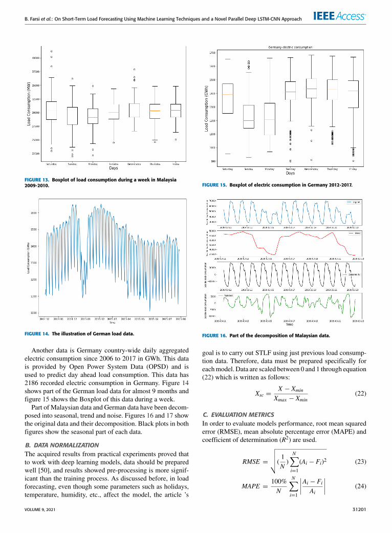
FIGURE 13. Boxplot of load consumption during a week in Malaysia2009-2010.

FIGURE 14. The illustration of German load data.

Another data is Germany country-wide daily aggregatedelectric consumption since 2006 to 2017 in GWh. This datais provided by Open Power System Data (OPSD) and isused to predict day ahead load consumption. This data has2186 recorded electric consumption in Germany. Figure 14shows part of the German load data for almost 9 months andfigure 15 shows the Boxplot of this data during a week.Part of Malaysian data and German data have been decom-

posed into seasonal, trend and noise. Figures 16 and 17 showthe original data and their decomposition. Black plots in bothfigures show the seasonal part of each data.

B. DATA NORMALIZATIONThe acquired results from practical experiments proved thatto work with deep learning models, data should be preparedwell [50], and results showed pre-processing is more signif-icant than the training process. As discussed before, in loadforecasting, even though some parameters such as holidays,temperature, humidity, etc., affect the model, the article ’s

FIGURE 15. Boxplot of electric consumption in Germany 2012-2017.

FIGURE 16. Part of the decomposition of Malaysian data.

goal is to carry out STLF using just previous load consump-tion data. Therefore, data must be prepared specifically foreachmodel. Data are scaled between 0 and 1 through equation(22) which is written as follows:

Xsc =X − Xmin

Xmax − Xmin(22)

C. EVALUATION METRICSIn order to evaluate models performance, root mean squarederror (RMSE), mean absolute percentage error (MAPE) andcoefficient of determination (R2) are used.

RMSE =

√√√√(1N)N∑i=1

(Ai − Fi)2 (23)

MAPE =100%N

N∑i=1

∣∣∣∣Ai − FiAi

∣∣∣∣ (24)

VOLUME 9, 2021 31201


FIGURE 17. Part of the decomposition of German data.

R2 = 1−SSRSST

(25)

SSR =N∑i=1

(Ai − Fi)2 (26)

SST =N∑i=1

(Ai − Ai)2 (27)

whereAi andFi refer to actual and predicted value of i-th data,N is the data size, A is the average of actual data. In addition,SSR stands for sum squared regression and SST stands fortotal sum of squared.

D. IMPLEMENTATIONIn this section, the results of all the discussed models arepresented.

1) THE EVALUATION OF ARIMAIn ARIMA models, time-series data decompose into m seriesto eliminate hourly/daily seasonality within data. Accordingto figures 10, 11 there is a daily seasonality in Malaysiandata (every 24 hours), and weekly seasonality in Germandata (every 7 days). Therefore, instead of using simpleARIMA, seasonal ARIMA (SARIMA) is being used to carryout STLF. In order to find the parameters of SARIMA,Auto-arima function from pmdarima library in python wasused and it tries to find the best number for parameters bycarrying out a comparison among different parameters. ForGerman data, ARIMA (5,1,0)(5,0,5,[7]) became the finalmodels and ARIMA (1,0,1)(2,0,0,[24]) achieved best resultsfor Malaysian data. Figures 18 and 19 illustrate predictedresults for both data from ARIMA model.

As can be seen, ARIMA carried out short-term loadforecasting for both daily and hourly data well. However,the problem is that for tuning the best parameters for ARIMAmodel, some complex computations must be solved. It leadsto a considerable amount of RAM involvement in addition tothe fact that it takes time.

FIGURE 18. Actual and predicted results from SARIMA, Malaysian data.

FIGURE 19. Actual and predicted results from SARIMA, German data.

2) THE EVALUATION OF EXPONENTIAL SMOOTHING:Exponential Smoothing (ETS) is an alternative approach forload forecasting. Training and test sets of two data sets areapplied to this model to carry out t + 1 forecasting. Besides,figures 20 and 21 show predicted and actual test set for bothdata. These plots prove that ETS fails to perform accuratelyin STLF.

3) THE EVALUATION OF LINEAR REGRESSIONFor the linear regression model, the ACF plot is used tofind out how many lags can be used as linear regressionvariables (independent data). In figure 22, ACF plot ofMalaysia is illustrated. For this data set, the threshold is 0.75.Lags [1, 2, 23, 24, 25, 47, 48, 49, 71, 72] become the inde-pendent data and actual load consumption are used as targets(dependent data). Scaled data is divided into training and testset. As 10 lags are used as variables, the shape of train set is(8723,10) which started from the first day of 2009 to the first

31202 VOLUME 9, 2021


FIGURE 20. Actual and predicted results from ETS, Malaysian data.

FIGURE 21. Actual and predicted results from ETS, German data.

day of 2010 and test set has the shape of (8723,10) from firstday of 2010 to the end of this year.

Figure 23 shows predicted and actual data of load con-sumption for year 2010 in Malaysia. As can be seen, linearregression achieved accurate results for this data set.

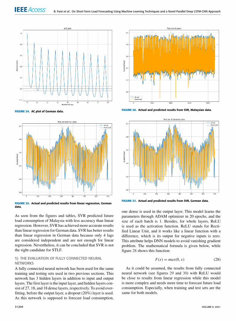
However, for the German data set, there are some dif-ferences. The first difference is that 0.69 is chosen for thethreshold. Figure 24 shows AC plot of German data. Accord-ing to this plot and threshold, lags [7, 14, 21, 28] are beingused as independent variables for MLR. Historical data from2012 to the end of 2015 are used as the training set. Theshape of training data is (1456,4), and the test set is from2016 to the end of 2017 with a shape of (702,4). As this datais daily, the model predicted daily load consumption but asnot good as predicted results from Malaysian data. Figure 25shows actual and predicted results from test set. Accordingto these figures, while linear regression can predict hourlyload series accurately, it fails to forecast accurately futureload consumption of daily load series. The difference in the

FIGURE 22. AC plot of Malaysian data.

FIGURE 23. Actual and predicted results from linear regression,Malaysian data.

number of lags as variables explains why the results are notsimilar. The number of variables (lags) for Malaysian datais 10, while it is 4 for German data. This point is the mainweakness of linear regression. Even though this model ishigh-speed, it fails to achieve accurate results if there is notmuch auto-correlation in input data.

4) THE EVALUATION OF SVRAs SVR is a regression-based approach, the same trainingand test sets for linear regression in the previous section areused to evaluate the model. Various parameters affect SVRto perform well. Among all these parameters, choosing theappropriate kernel has the most importance. For Malaysiandata, the ’linear’ kernel had the best performance compared toother kernels, and the German case selects ’radial bias func-tion (rbf)’ as kernel according to its well-performance withthis data set. In addition, figures 26 and 27 show the predictedload consumption from SVR for both data sets, respectively.

VOLUME 9, 2021 31203


FIGURE 24. AC plot of German data.

FIGURE 25. Actual and predicted results from linear regression, Germandata.

As seen from the figures and tables, SVR predicted futureload consumption of Malaysia with less accuracy than linearregression. However, SVR has achievedmore accurate resultsthan linear regression for German data. SVR has better resultsthan linear regression in German data because only 4 lagsare considered independent and are not enough for linearregression. Nevertheless, it can be concluded that SVR is notthe right candidate for STLF.

5) THE EVALUATION OF FULLY CONNECTED NEURALNETWORKSA fully connected neural network has been used for the sametraining and testing sets used in two previous sections. Thisnetwork has 3 hidden layers in addition to input and outputlayers. The first layer is the input layer, and hidden layers con-sist of 27, 18, and 18 dense layers, respectively. To avoid over-fitting, before the output layer, a dropout (20%) layer is used.As this network is supposed to forecast load consumption,

FIGURE 26. Actual and predicted results from SVR, Malaysian data.

FIGURE 27. Actual and predicted results from SVR, German data.

one dense is used in the output layer. This model learns theparameters through ADAM optimizer in 20 epochs, and thesize of each batch is 1. Besides, for whole layers, ReLUis used as the activation function. ReLU stands for Recti-fied Linear Unit, and it works like a linear function with adifference, which is its output for negative inputs is zero.This attribute helps DNN models to avoid vanishing gradientproblem. The mathematical formula is given below, whilefigure 28 shows this function:

F(x) = max(0, x) (28)

As it could be assumed, the results from fully connectedneural network (see figures 29 and 30) with ReLU wouldbe close to results from linear regression while this modelis more complex and needs more time to forecast future loadconsumption. Especially, when training and test sets are thesame for both models.

31204 VOLUME 9, 2021


FIGURE 28. ReLU illustrative function.

FIGURE 29. Actual and predicted results from fully connected, Malaysiandata.

6) THE EVALUATION OF LSTMIn this article, the LSTM model studies the last 24 hoursload consumption and predict the next hour consumptionin Malaysian data. In contrast, in German data, in order topredict next-day load consumption, it studies the last 7 daysand predicts next day data. It has one LSTM layer in termsof architecture, while one dense layer is used as output.This type of architecture calls Vanilla LSTM, a well-knownnetwork and widely used in different areas. Same with thefully connected network in the previous section, the usedactivation function is ReLU. The model is also trained byADAM optimizer for Malaysian data in 200 epochs andRMSprop for German data in 150 epochs. This model provesthat LSTMs are a powerful tool for STLF due to the accurateresults that the LSTM model has achieved as well as theirindependence to auto-correlation of input data. The resultsare illustrated in figures 31 and 32.

FIGURE 30. Actual and predicted results from fully connected, Germandata.

FIGURE 31. Actual and predicted load consumption from LSTM,Malaysian data.

7) THE EVALUATION OF CNN-LSTM AND PLCNetAs discussed before, CNNs are well-known networks forfeature extraction. LSTM also showed its ability to predictshort-term load consumption. Therefore, a hybrid model ofCNN and LSTM can come with several advantages. In orderto work with this hybrid model, CNN layers should be imple-mented first to apply historical data. In the next step, extractedfeatures from CNNs are used as input for LSTM layers. Thissection uses a 7-layer model to apply on the same test andtraining set used for the LSTMmodel in the previous section.In layer #1 and layer #2, 1-D CNNs with the ReLU activationfunction and filters= 64 and kernel size= 3 are implemented.After that, a Maxpooling and Flatten layer are used to preparedata for the LSTM layer. In layer #5, 200 LSTM neuronswith ReLU activation function are implemented. Two denselayers with 200 and 1 neurons are implemented to analyze theresults and predict load consumption, while ReLU is used as

VOLUME 9, 2021 31205


FIGURE 32. Actual and predicted load consumption from LSTM, Germandata.

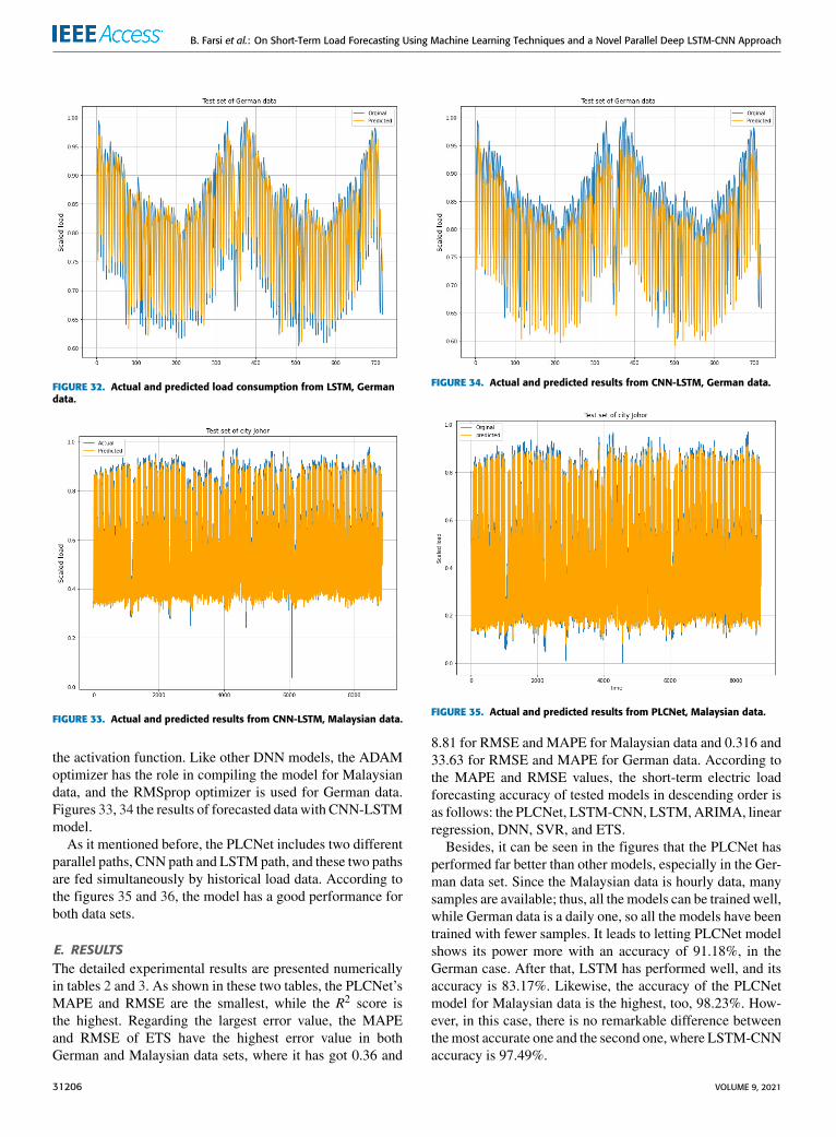
FIGURE 33. Actual and predicted results from CNN-LSTM, Malaysian data.

the activation function. Like other DNN models, the ADAMoptimizer has the role in compiling the model for Malaysiandata, and the RMSprop optimizer is used for German data.Figures 33, 34 the results of forecasted data with CNN-LSTMmodel.

As it mentioned before, the PLCNet includes two differentparallel paths, CNN path and LSTMpath, and these two pathsare fed simultaneously by historical load data. According tothe figures 35 and 36, the model has a good performance forboth data sets.

E. RESULTSThe detailed experimental results are presented numericallyin tables 2 and 3. As shown in these two tables, the PLCNet’sMAPE and RMSE are the smallest, while the R2 score isthe highest. Regarding the largest error value, the MAPEand RMSE of ETS have the highest error value in bothGerman and Malaysian data sets, where it has got 0.36 and

FIGURE 34. Actual and predicted results from CNN-LSTM, German data.

FIGURE 35. Actual and predicted results from PLCNet, Malaysian data.

8.81 for RMSE and MAPE for Malaysian data and 0.316 and33.63 for RMSE and MAPE for German data. According tothe MAPE and RMSE values, the short-term electric loadforecasting accuracy of tested models in descending order isas follows: the PLCNet, LSTM-CNN, LSTM,ARIMA, linearregression, DNN, SVR, and ETS.

Besides, it can be seen in the figures that the PLCNet hasperformed far better than other models, especially in the Ger-man data set. Since the Malaysian data is hourly data, manysamples are available; thus, all the models can be trained well,while German data is a daily one, so all the models have beentrained with fewer samples. It leads to letting PLCNet modelshows its power more with an accuracy of 91.18%, in theGerman case. After that, LSTM has performed well, and itsaccuracy is 83.17%. Likewise, the accuracy of the PLCNetmodel for Malaysian data is the highest, too, 98.23%. How-ever, in this case, there is no remarkable difference betweenthemost accurate one and the second one, where LSTM-CNNaccuracy is 97.49%.

31206 VOLUME 9, 2021


FIGURE 36. Actual and predicted results from PLCNet, German data.

TABLE 2. Models Performance for Malaysian Data.

TABLE 3. Models Performance for German Data.

TABLE 4. The Training Time Per Epoch of Deep Learning Models.

Regarding the run time in the tables, linear regressionand SVR are the fastest in German and Malaysian cases.However, they are outperformed by deep learning models.Besides, ARIMA and ETS are two computational techniquesthat take significant time for training. Even though all deeplearning models in the tables took much time to be trainedcompared to regression-based approaches, their acquiredaccuracy is acceptable. The difference between the trainingtime in deep learning models depends on the number ofepochs considered. Table 4 indicates the runtime per epoch

FIGURE 37. Histogram plot of the PLCNet results for Malaysian data.

of each deep learning model for both Malaysian and Germandata sets. According to the tables 2 and 3, LSTM has thehighest runtime, but the main reason is that this model needsmore epochs to be trained and predict future load. It can beseen that in table 4 LSTM is faster than LSTM-CNN andDNN models in both data sets. However, the PLCNet resultsshow that this model has the highest accuracy and lowest erroramount. It is also the fastest model between deep learningmodels where the runtime per epoch in Malaysian data is4.5(s) and in German data is 0.93(s).

Therefore, it is proven that the novel hybrid STLF algo-rithm proposed in this article is practical and useful. AlthoughLSTM has a good performance when dealing with time-series, its accuracy in German data set, which does not havemany samples, is not good enough. Therefore, the LSTM isnot suitable for this kind of prediction. Finally, the experimen-tal results show that the PLCNet provides the best electricityload forecasting results.

F. STATISTICAL ANALYSISA common approach to comparing the performance of themachine learning models is using statistical methods to selectthe best one. This section aims to compare the PLCNet, andLSTM results since both achieved acceptable results in bothGerman and Malaysian cases. To provide statistical analysisof the PLCNet and LSTM results, these two models were run10 times. In terms of visualization, figures 37 and 38 showthe results histogram of the PLCNet and LSTM forMalaysiandata set, respectively.

In this section, the t-test is used to understand the achievedresults are just some stochastic results or they are trustfulto perform statistical analysis. This analysis works based onthe null hypothesis. The null hypothesis is that two models(the PLCNet and LSTM) are similar to each other. There isno difference between them, while the alternative hypothesisis that the two models perform differently. The consideredsignificance level is 5%, so if the acquired P-value is less than

VOLUME 9, 2021 31207


FIGURE 38. Histogram plot of LSTM results for Malaysian data.

FIGURE 39. Histogram plot of the PLCNet results for German data.

5%, the null hypothesis can be rejected. It can be concludedthat the PLCNet performs better than the LSTMmodel. Aftercarrying out some statistical analysis, the obtained P-valueis 0.0411 (or 4.11%), less than 5%. Likewise, after applyingthe statistical analysis to the German data case, it can beconcluded that the results from the PLCNet are not stochas-tic, where the obtained P-value is 0.03019 (or 3.019%).Figures 38 and 39 illustrate the histogram plot of the results.

G. DIFFERENT TIME HORIZONSPrevious sections discussed some machine learning tech-niques to predict next time step load data consumption.In other words, at time t , they predicted the load data attime t + 1. Since the Malaysian data is hourly data andGerman data is a daily one, all the models predicted the nexthour load of Malaysian data and the next-day German dataload. This section aims to challenge the PLCNet in differenthorizons. In the Malaysian case, the PLCNet will predict thenext 24 hours, next 48 hours, and next 10 days load data,

FIGURE 40. Histogram plot of LSTM results for German data.

and in the German case, it will predict next 7 days, next10 days, and next 30 days. RMSE and R2 scores are the twometrics used to evaluate the model’s performance in termsof evaluation. Because of the existing soft computing errors,the model is tested 5 times for each horizon, and the averagevalue is calculated. Same asmentioned before, themodel usesthe year 2009 as training set and year 2010 as the test set inMalaysian data, and years 2012-2015 are used as the trainingset and 2016-2017 as the test set in the German data set.

1) MALAYSIAN CASESince in previous sections, the prediction of next hour loaddata through the PLCNet was discussed thoroughly, thissection studies the next one day, 2 days, and 10 days loaddata in the following.

The Malaysian data is hourly data, so predicting one dayahead load data next 24 time steps should be predicted,leading to a subtle modification in the model’s architecture.The last layer of the model, which is a dense layer, will have24 neurons to provide the next 24 hours prediction. To predictone-day data, the model looks back to 72 hours ago to trainthe algorithm within data and then predict the next 24 hours.Figure 41 shows the results of the prediction.

In order to forecast the next 2 days load data, the next48 time steps should be predicted, so another modification isneeded to make the model able to forecast the next days’ loaddata. Thus, the model will have 48 neurons in its last layer(a dense layer). In terms of the training procedure, the modellooks back to 4 days ago (4days×24h) to be trained, and thenit predicts the next 2 days. Figure 42 illustrates the predictionand actual load data.

This paragraph aims to predict the next 10 days of loaddata, an MTLF task but a big challenge for the model. Sincethe samples have been recorded hourly in Malaysian data,the model must predict 240 values (10 days × 24h). Thereare 240 neurons in the last layer. The model looks back to10 days ago and predicts 10 days ahead load data in thetraining process. According to figure 43, the results show that

31208 VOLUME 9, 2021


FIGURE 41. 1 day ahead results using the PLCNet, Malaysian data.

FIGURE 42. 2 days ahead results using the PLCNet, Malaysian data.

the PLCNet has an acceptable performance in this task wherethe results are close to next hour, one day and 2 days aheadoutputs.

2) RESULTSTables 5 and 6 show the results of next days prediction.However, to have comprehensive knowledge in terms of themodel’s performance, the results of the next hour predictionare added to these tables again. In this table, A1, A2, A3 andA4 represent next hour, next day, next 2 days and next 10 daysresults.

Even though forecasting future load data in longer timehorizons is a challenging task, according to these tables, thereis almost 4% difference between the accuracy of the nexthour prediction and the next 10 days prediction which is anacceptable difference and the model has a good performancein Malaysian case.

Likewise, in order to make sure the PLCNet has betterperformance rather than two other discussed deep learning

FIGURE 43. 10 days ahead results using the PLCNet, Malaysian data.

TABLE 5. The Experimental Results of Malaysian Data in Terms of R2

Score.

TABLE 6. The Experimental Results of Malaysian Data in Terms of RMES.

TABLE 7. The Comparison Table for Malaysian Data in Terms of R2 Score.

TABLE 8. The Comparison Table for Malaysian Data in Terms of RMSE.

models including DeepEnergy [20], LSTM and CNN-LSTM,tables 7 and 8 are provided to compare the results of all thesemodels in different time horizons in terms of RMSE and R2

score.

3) GERMAN CASESame as Malaysian data, the model is challenged throughGerman data set but in different time horizons. It predicts thenext 7 days, next 10 days, and next 30 days load data.

The model looks back to 7 days ago to perform 7 daysahead prediction and to do this task it needs 7 neurons in itslast layer. Figure 44 shows the result of using the PLCNet toforecast Germany’s next 7 days load data.

VOLUME 9, 2021 31209


FIGURE 44. 7 days ahead results using the PLCNet, German data.

FIGURE 45. 10 days ahead results using the PLCNet model, German data.

This paragraph discusses the results of 10 days aheadprediction. As the model is supposed to predict next 10 days,there are 10 neurons in the last layer of the model. Besides,since forecasting the next days data is a bit harder thannext 7 days, the model looks back to 10 days ago data tounderstand the algorithmwithin load series better. The resultsare shown in figure 45.If the PLCNet can carry out an LTLF task, it can be

introduced as a well-performance tool in load forecastingapplications. To evaluate the LTLF taskmodel’s performance,this section aims to predict the next 30 days of German loaddata, and the results are shown in figure 46. Like previoussections, there are 30 neurons in the last layer of the model topredict future load data in terms of the model architecture.

4) RESULTSSo far, the German data set’s illustrative results have beenshown, and in the following, the numerical results areavailable. Besides, the one day ahead prediction results are

FIGURE 46. 30 days ahead results using the PLCNet, German data.

TABLE 9. The Experimental Results of German Data in Terms of R2 Score.

TABLE 10. The Experimental Results of German Data in Terms of RMES.

TABLE 11. The Comparison Table for German Data in Terms of R2 Score.

available in tables 10 and 9 to demonstrate the comparisonbetween different horizons for same data sets. Themodeling’sname B1, B2, B3, and B4 represent the modeling for 1, 7,10, and 30 days ahead, respectively. These two tables indi-cate that there are not many differences between one dayahead prediction and 10 days ahead prediction. Still, it isa big challenge for the model to predict the next 30 daysload series because the average accuracy for the next dayprediction is 91.31% while it is 82.49% for the next 30 daysprediction. The problem is that the German data is not abig data set, and it has only 2186 recorded samples, so itis difficult for the model to learn all the parameters wellwhile looking back 30 previous steps and predicting the next30 steps.

Same as the Malaysian data, a comparison table(see tables 11 and 12) is provided for German results to provethat the PLCNet not only has a better performance in one stepahead prediction but also it can perform better than other deeplearning models in different time horizons.

31210 VOLUME 9, 2021


TABLE 12. The Comparison Table for German Data in Terms of RMSE.

IV. CONCLUSIONWith smart grids on the rise, the importance of short-termload forecasting highly increases. To predict the future loadconsumption, some factors such as weather can affect theresults. The lack of future weather is a challenging problemfor load forecasting. In this article, the previous consumptionwas used as a parameter to predict the load one step ahead.Some non-deep learning approaches like linear regressionor ARIMA have proven powerful tools for accurate loadforecasting. However, regression-based methods come withsome disadvantages. In order to use these models, suchas SVR and linear regression, lags are used as parametersthrough auto-correlation (AC) values. As the threshold valueis subjective, the number of lags as regression-based mod-els’ parameters can be different. Fully connected networksalso use the same approach as regression-based approaches.Because there is no constant threshold to find those lagsthat are suitable to be used as variables, this procedure(finding lags through AC plot) may lead to higher errors.ARIMA and ETS also are two well-known time-series anal-ysis approaches. However, some parameters need to be tunedto work with these methods. This procedure needs numeroustrials to find the best values for them. Furthermore, in time-series methods, data must be analyzed to find out if they arestationary or not. In contrast, LSTM can achieve good resultswhether data is stationary or not. CNN-LSTM also is a hybridmodel, which is used in various load forecasting studies.The PLCNet achieves the best results between all the dis-cussed models where the accuracy increase from 83.17% to91.18% for load data in a German case study. Likewise, for aMalaysian data set, the model’s obtained accuracy is 98.23%which is very high for time-series results and the RMSE isvery low at 0.031. In summary, the PLCNet improves theresults remarkably for the German data set. Besides, whileall the models have acceptable Malaysian data performance,the most accurate results come from the PLCNet. It is fasterthan other deep learning models to train both German andMalaysian data in terms of runtime. This improvement andhighly accurate results, as well as a quick training process,prove that this novel hybrid model is a good choice for STLFtasks. The PLCNetmodel was also evaluated in different hori-zons, and it performed better than other deep learningmodels.The accuracy of the PLCNet in Malaysian experiments fordifferent horizons is between 94.16% and 98.14%. In Germandata, it is between 82.49% and 91.31%, which are acceptableresults compared to other deep learning models’ results.

The interest in using artificial neural networks for electricload forecasting is winning ground in research and industries,especially when deployed in IoT applications. According tothe discussed results, deep learning models can be the right

choice for IoT compared to other techniques. Thus furtherwork could be devoted to using deep learning models such asthe PLCNet in this article for online load forecasting tasks.

REFERENCES[1] World Energy Outlook 2019, IEA, Paris, France, 2019, doi: 10.1787/

caf32f3b-en.[2] H. Daki, A. E. Hannani, A. Aqqal, A. Haidine, and A. Dahbi, ‘‘Big data

management in smart grid: Concepts, requirements and implementation,’’J. Big Data, vol. 4, no. 1, pp. 1–19, Dec. 2017, doi: 10.1186/s40537-017-0070-y.

[3] S. Acharya, Y. Wi, and J. Lee, ‘‘Short-term load forecasting for a singlehousehold based on convolution neural networks using data augmenta-tion,’’ Energies, vol. 12, no. 18, p. 3560, Sep. 2019.

[4] X. Fang, S. Misra, G. Xue, and D. Yang, ‘‘Smart grid—The new andimproved power grid: A survey,’’ IEEE Commun. Surveys Tuts., vol. 14,no. 4, pp. 944–980, 4th Quart., 2012.

[5] J. Sharp, ‘‘Book reviews,’’ Int. J. Forecasting, vol. 2, no. 2, pp. 241–242,1986.

[6] V. Gupta, ‘‘An overview of different types of load forecasting methodsand the factors affecting the load forecasting,’’ Int. J. Res. Appl. Sci. Eng.Technol., vol. 5, no. 4, pp. 729–733, Apr. 2017.

[7] L. Ekonomou, C. A. Christodoulo, and V. Mladenov, ‘‘A short-term loadforecasting method using artificial neural networks and wavelet analysis,’’Int. J. Power Syst., vol. 1, pp. 64–68, Jul. 2016.

[8] F. Javed, N. Arshad, F. Wallin, I. Vassileva, and E. Dahlquist, ‘‘Forecast-ing for demand response in smart grids: An analysis on use of anthro-pologic and structural data and short term multiple loads forecasting,’’Appl. Energy, vol. 96, pp. 150–160, Aug. 2012, doi: 10.1016/j.apenergy.2012.02.027.

[9] C. Xia, J. Wang, and K. Mcmenemy, ‘‘Short, medium and long termload forecasting model and virtual load forecaster based on radial basisfunction neural networks,’’ Int. J. Electr. Power Energy Syst., vol. 32, no. 7,pp. 743–750, Sep. 2010.

[10] J. Gehring, M. Auli, D. Grangier, D. Yarats, and Y. N. Dauphin, ‘‘Convolu-tional sequence to sequence learning,’’ 2017, arXiv:1705.03122. [Online].Available: http://arxiv.org/abs/1705.03122

[11] A. van den Oord, S. Dieleman, H. Zen, K. Simonyan, O. Vinyals,A. Graves, N. Kalchbrenner, A. Senior, and K. Kavukcuoglu, ‘‘WaveNet:A generative model for raw audio,’’ 2016, arXiv:1609.03499. [Online].Available: https://arxiv.org/abs/1609.03499

[12] R. Yamashita, M. Nishio, R. K. G. Do, and K. Togashi, ‘‘Convolutionalneural networks: An overview and application in radiology,’’ InsightsImag., vol. 9, no. 4, pp. 611–629, Aug. 2018, doi: 10.1007/s13244-018-0639-9.

[13] A. Gasparin and C. Alippi, ‘‘Deep learning for time series forecasting:The electric load case,’’ 2019, arXiv:1907.09207. [Online]. Available:https://arxiv.org/abs/1907.09207

[14] B. Yildiz, J. I. Bilbao, and A. B. Sproul, ‘‘A review and analysis ofregression andmachine learningmodels on commercial building electricityload forecasting,’’ Renew. Sustain. Energy Rev., vol. 73, pp. 1104–1122,Jun. 2017.

[15] C. Tian, J. Ma, C. Zhang, and P. Zhan, ‘‘A deep neural network modelfor short-term load forecast based on long short-term memory networkand convolutional neural network,’’ Energies, vol. 11, no. 12, p. 3493,Dec. 2018.

[16] W. He, ‘‘Load forecasting via deep neural networks,’’ Procedia Comput.Sci., vol. 122, pp. 308–314, 2017, doi: 10.1016/j.procs.2017.11.374.

[17] C. Gallicchio and A. Micheli, ‘‘Deep echo state network (Deep-ESN): A brief survey,’’ 2017, arXiv:1712.04323. [Online]. Available:http://arxiv.org/abs/1712.04323

[18] G. Zhang, B. E. Patuwo, and M. Y. Hu, ‘‘Forecasting with artificial neuralnetworks: The state of the art,’’ Int. J. Forecast., vol. 14, pp. 35–62,Mar. 1998.

[19] M. Q. Raza and A. Khosravi, ‘‘A review on artificial intelligence basedload demand forecasting techniques for smart grid and buildings,’’ Renew.Sustain. Energy Rev., vol. 50, pp. 1352–1372, Oct. 2015.

[20] P.-H. Kuo and C.-J. Huang, ‘‘A high precision artificial neural networksmodel for short-term energy load forecasting,’’ Energies, vol. 11, no. 1,p. 213, Jan. 2018, doi: 10.3390/en11010213.

[21] A. Liaw and M. Wiener, ‘‘Classification and Regression by random For-est,’’ R News, vol. 2, no. 3, pp. 18–22, 2002.

VOLUME 9, 2021 31211

http://dx.doi.org/10.1787/caf32f3b-en

http://dx.doi.org/10.1787/caf32f3b-en

http://dx.doi.org/10.1186/s40537-017-0070-y

http://dx.doi.org/10.1186/s40537-017-0070-y

http://dx.doi.org/10.1016/j.apenergy.2012.02.027

http://dx.doi.org/10.1016/j.apenergy.2012.02.027

http://dx.doi.org/10.1007/s13244-018-0639-9

http://dx.doi.org/10.1007/s13244-018-0639-9

http://dx.doi.org/10.1016/j.procs.2017.11.374

http://dx.doi.org/10.3390/en11010213


[22] C. Gerwig, ‘‘Short term load forecasting for residential buildings—Anextensive literature review,’’ in Intelligent Decision Technologies. IDT(Smart Innovation, Systems and Technologies), vol. 39, R. Neves-Silva,L. Jain, and R. Howlett, Eds. Cham, Switzerland: Springer, 2017.

[23] L. Hu and G. Taylor, ‘‘A novel hybrid technique for short-term electricityprice forecasting in UK electricity markets,’’ J. Int. Council Electr. Eng.,vol. 4, no. 2, pp. 114–120, Apr. 2014, doi: 10.5370/JICEE.2014.4.2.114.

[24] C.-J. Huang and P.-H. Kuo, ‘‘Multiple-input deep convolutional neural net-work model for short-term photovoltaic power forecasting,’’ IEEE Access,vol. 7, pp. 74822–74834, 2019, doi: 10.1109/ACCESS.2019.2921238.

[25] H. J. Sadaei, P. C. D. L. E. Silva, F. G. Guimarães, and M. H. Lee,‘‘Short-term load forecasting by using a combinedmethod of convolutionalneural networks and fuzzy time series,’’ Energy, vol. 175, pp. 365–377,May 2019.

[26] F. M. Bianchi, E. Maiorino, M. C. Kampmeyer, A. Rizzi, and R. Jenssen,Recurrent Neural Networks for Short-Term Load Forecasting (Springer-Briefs in Computer Science). Springer, 2017, doi: 10.1007/978-3-319-70338-1.

[27] R. M. Pratapa and A. Laxmi, ‘‘IOT based online load forecastingusing machine learning algorithms,’’ Procedia Comput. Sci., vol. 171,pp. 551–560, 2020, doi: 10.1016/j.procs.2020.04.059.

[28] N. Amjady, ‘‘Short-term hourly load forecasting using time-series model-ingwith peak load estimation capability,’’ IEEE Trans. Power Syst., vol. 16,no. 4, pp. 798–805, Nov. 2001, doi: 10.1109/59.962429.

[29] P. Ji, D. Xiong, P. Wang, and J. Chen, ‘‘A study on exponential smoothingmodel for load forecasting,’’ in Proc. Asia–Pacific Power Energy Eng.Conf., Mar. 2012, pp. 1–4.

[30] M. D. Reddy and N. Vishali, ‘‘Load forecasting using linear regressionanalysis in time series model for RGUKT, RK valley campus HT feeder,’’Int. J. Eng. Res. Technol., vol. 6, no. 5, pp. 624–625, 2017.

[31] G. Dudek, ‘‘Pattern-based local linear regression models for short-term load forecasting,’’ Electr. Power Syst. Res., vol. 130, pp. 139–147,Jan. 2016.

[32] E. Ceperic, V. Ceperic, and A. Baric, ‘‘A strategy for short-term loadforecasting by support vector regression machines,’’ IEEE Trans. PowerSyst., vol. 28, no. 4, pp. 4356–4364, Nov. 2013.

[33] B.-J. Chen, M.-W. Chang, and C.-J. Lin, ‘‘Load forecasting using supportvector machines: A study on EUNITE competition 2001,’’ IEEE Trans.Power Syst., vol. 19, no. 4, pp. 1821–1830, Nov. 2004.

[34] H. S. Hippert, C. E. Pedreira, and R. C. Souza, ‘‘Neural networks for short-term load forecasting: A review and evaluation,’’ IEEE Trans. Power Syst.,vol. 16, no. 1, pp. 44–55, Feb. 2001.

[35] X. Ying, ‘‘An overview of overfitting and its solutions,’’ J. Phys.,Conf. Ser., vol. 1168, Feb. 2019, Art. no. 022022, doi: 10.1088/1742-6596/1168/2/022022.

[36] S. Ruder, ‘‘An overview of gradient descent optimization algorithms,’’2016, arXiv:1609.04747. [Online]. Available: http://arxiv.org/abs/1609.04747

[37] D. P. Kingma and J. L. Ba, ‘‘Adam: Amethod for stochastic optimization,’’in Proc. 3rd Int. Conf. Learn. Represent. (ICLR), San Diego, CA, USA,May 2015. [Online]. Available: http://arxiv.org/abs/1412.6980

[38] S. Hochreiter and J. Schmidhuber, ‘‘Long short-term memory,’’ NeuralComput., vol. 9, no. 8, pp. 1735–1780, 1997.

[39] Z. Che, S. Purushotham, K. Cho, D. Sontag, and Y. Liu, ‘‘Recurrent neuralnetworks formultivariate time series withmissing values,’’ Sci. Rep., vol. 8,no. 1, pp. 1–12, Dec. 2018.

[40] S. Muzaffar and A. Afshari, ‘‘Short-term load forecasts using LSTMnetworks,’’ Energy Procedia, vol. 158, pp. 2922–2927, Feb. 2019.

[41] B.-S. Kwon, R.-J. Park, and K.-B. Song, ‘‘Short-term load forecastingbased on deep neural networks using LSTM layer,’’ J. Electr. Eng. Technol.,vol. 15, no. 4, pp. 1501–1509, Jul. 2020.

[42] Y. Lecun, L. Bottou, Y. Bengio, and P. Haffner, ‘‘Gradient-based learn-ing applied to document recognition,’’ Proc. IEEE, vol. 86, no. 11,pp. 2278–2324, Nov. 1998.

[43] A. Krizhevsky, I. Sutskever, and G. E. Hinton, ‘‘ImageNet classificationwith deep convolutional neural networks,’’ in Advances in Neural Infor-mation Processing Systems 25. Red Hook, NY, USA: Curran Associates,2012, pp. 1097–1105.

[44] R. Girshick, ‘‘Fast R-CNN,’’ in Proc. IEEE Int. Conf. Comput. Vis. (ICCV),Dec. 2015, pp. 1440–1448.

[45] K. Noda, Y. Yamaguchi, K. Nakadai, H. G. Okuno, and T. Ogata, ‘‘Audio-visual speech recognition using deep learning,’’ Appl. Intell., vol. 42, no. 4,pp. 722–737, 2015.

[46] F. Milletari, N. Navab, and S.-A. Ahmadi, ‘‘V-Net: Fully convolutionalneural networks for volumetric medical image segmentation,’’ in Proc. 4thInt. Conf. 3D Vis. (3DV), Oct. 2016, pp. 565–571.

[47] B. Stephen, X. Tang, P. R. Harvey, S. Galloway, and K. I. Jennett, ‘‘Incor-porating practice theory in sub-profile models for short term aggregatedresidential load forecasting,’’ IEEE Trans. Smart Grid, vol. 8, no. 4, pp.1591–1598, Jul. 2017, doi: 10.1109/TSG.2015.2493205.

[48] A. Z. Hinchi and M. Tkiouat, ‘‘Rolling element bearing remaining usefullife estimation based on a convolutional long-short-term memory net-work,’’ Procedia Comput. Sci., vol. 127, 2018, Art. no. 123132.

[49] N. Srivastava, R. Salakhutdinov, A. Krizhevsky, I. Sutskever, andG. Hinton, ‘‘Dropout: A simple way to prevent neural networks fromoverfitting,’’ J. Mach. Learn. Res., vol. 15, no. 1, pp. 1929–1958, 2014.

[50] J. Sola and J. Sevilla, ‘‘Importance of input data normalization for theapplication of neural networks to complex industrial problems,’’ IEEETrans. Nucl. Sci., vol. 44, no. 3, pp. 1464–1468, Jun. 1997, doi: 10.1109/23.589532.

[51] J. Li, X. Li, and D. He, ‘‘A directed acyclic graph network combined withCNN and LSTM for remaining useful life prediction,’’ IEEE Access, vol. 7,pp. 75464–75475, 2019, doi: 10.1109/ACCESS.2019.2919566.

BEHNAM FARSI received the bachelor’s degreefrom the Electrical Engineering Department, Fer-dowsi University, Iran, in 2019. He is currentlypursuing the master’s degree with the Concor-dia Institute for Information Systems Engineer-ing (CIISE) Department, Concordia University,Canada. His master’s thesis topic was on loadforecasting. His research interests includemachinelearning, deep learning, load forecasting, andremaining useful life prediction.

MANAR AMAYRI received the bachelor’s degreein power engineering from Damascus University,Syria, the master’s degree in electrical power sys-tems from the Power Department, Damascus Uni-versity, the master’s degree in smart grids andbuildings from ENES3, INP-Grenoble (InstituteNational Polytechnique de Grenoble), in 2014, andthe Ph.D. degree in energy smart-buildings fromthe Grenoble Institute of Technology, in 2017. Sheis currently an Assistant Professor with ENES3,

INP-Grenoble, G-SCOP Lab (Sciences pour la conception, l’Optimisationet la Production).

NIZAR BOUGUILA (Senior Member, IEEE)received the Engineer degree from the Univer-sity of Tunis, Tunis, Tunisia, in 2000, and theM.Sc. and Ph.D. degrees in computer science fromSherbrooke University, Sherbrooke, QC, Canada,in 2002 and 2006, respectively. He is currently aProfessor with the Concordia Institute for Infor-mation Systems Engineering (CIISE), ConcordiaUniversity, Montreal, QC, Canada. His researchinterests include machine learning, data mining,

computer vision, and pattern recognition applied to different real-lifeproblems.

URSULA EICKER has held leadership positions asa German Physicist with the Centre for Sustain-able Energy Technologies, Stuttgart University ofApplied Sciences. Since June 2019, she has beenleading an ambitious research program to estab-lish transformation strategies toward zero-carboncities. She is currently the Canada ExcellenceResearch Chair (CERC) for Next GenerationCities with Concordia University, Montreal. Hercurrent research interests include urban scale mod-

eling, zero carbon buildings, renewable energies, and circular economystrategies.

31212 VOLUME 9, 2021

http://dx.doi.org/10.5370/JICEE.2014.4.2.114

http://dx.doi.org/10.1109/ACCESS.2019.2921238

http://dx.doi.org/10.1007/978-3-319-70338-1

http://dx.doi.org/10.1007/978-3-319-70338-1

http://dx.doi.org/10.1016/j.procs.2020.04.059

http://dx.doi.org/10.1109/59.962429

http://dx.doi.org/10.1088/1742-6596/1168/2/022022

http://dx.doi.org/10.1088/1742-6596/1168/2/022022

http://dx.doi.org/10.1109/TSG.2015.2493205

http://dx.doi.org/10.1109/23.589532

http://dx.doi.org/10.1109/23.589532

http://dx.doi.org/10.1109/ACCESS.2019.2919566

On Short-Term Load Forecasting Using Machine Learning ...

Documents

Transcript of On Short-Term Load Forecasting Using Machine Learning ...