SHIP FORM CALCULATIONS

It has been seen that the three dimensional hull form can be

represented by a series of curves which are the intersections of the

hull with three sets of mutually orthogonal planes. The naval

architect is interested in the areas and volumes enclosed by the

curves and surfaces so represented.

The naval architect is constantly required to find the area, centroids of

areas, first moment of area and second moment of area (moment of

inertia) of figures bounded by straight lines and curves. There are

various rules in common use for finding areas such as Trapezoidal rule,

Simpson’s First Rule, Simpson’s Second Rule etc.

To find the centroids of the areas and volumes it is necessary to

obtain their first moments of the area about chosen axes (x, y, z).

For some hydrostatic calculations, the moments of inertia (second

moment ) of the areas are needed. This is obtained from the second

moment of the area, again about chosen axes.

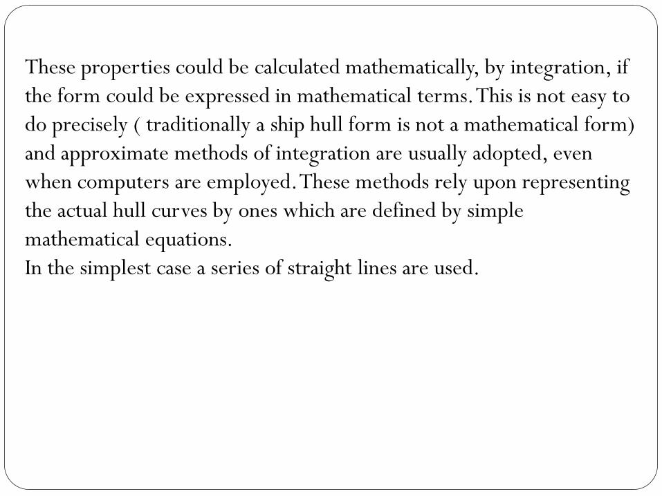
These properties could be calculated mathematically, by integration, if

the form could be expressed in mathematical terms. This is not easy to

do precisely ( traditionally a ship hull form is not a mathematical form)

and approximate methods of integration are usually adopted, even

when computers are employed. These methods rely upon representing

the actual hull curves by ones which are defined by simple

mathematical equations.

In the simplest case a series of straight lines are used.

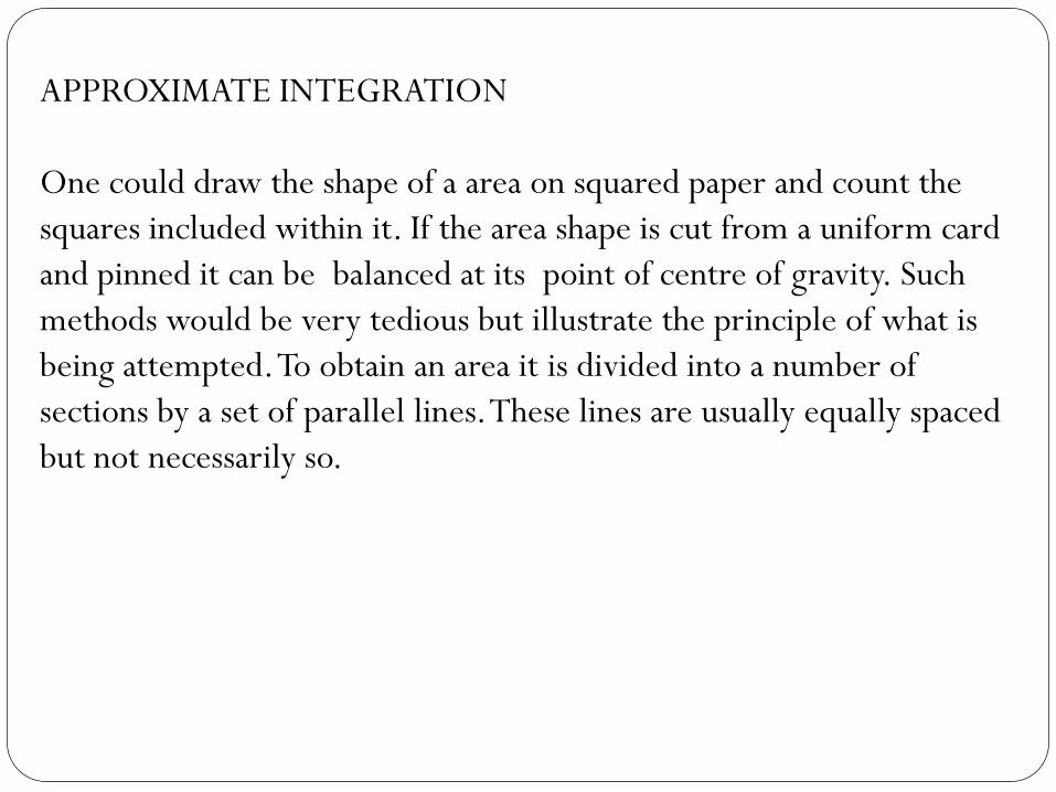
APPROXIMATE INTEGRATION

One could draw the shape of a area on squared paper and count the

squares included within it. If the area shape is cut from a uniform card

and pinned it can be balanced at its point of centre of gravity. Such

methods would be very tedious but illustrate the principle of what is

being attempted. To obtain an area it is divided into a number of

sections by a set of parallel lines. These lines are usually equally spaced

but not necessarily so.

TRAPEZOIDAL RULE

If the points at which the parallel lines intersect the area perimeter

are joined by straight lines, the area can be represented

approximately by the summation of the set of trapezia so formed.

The generalized form is illustrated like this:

The area of the shaded trapezium is:

A n

h n

The curve ABC has been replaced by two straight lines, AB and BC with

ordinates y y and y distance h apart. The area is the sum of the two

trapezia so formed 0 1 2

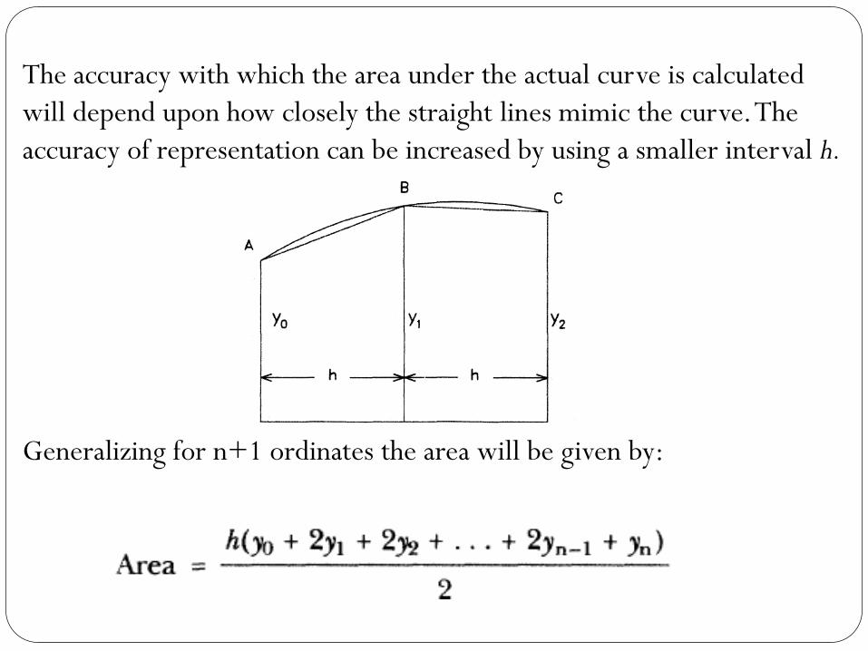
The accuracy with which the area under the actual curve is calculated

will depend upon how closely the straight lines mimic the curve. The

accuracy of representation can be increased by using a smaller interval h.

Generalizing for n+1 ordinates the area will be given by:

In many cases of ships' waterplanes, it is sufficiently accurate to use

ten divisions with eleven ordinates but it is worth checking by eye

whether the straight lines follow the actual curves reasonably

accurately.

Because warship hulls tend to have greater curvature they are usually

represented by twenty divisions with twenty-one ordinates.

To calculate the volume of a three dimensional shape the cross

sectional areas at equally spaced intervals can be calculated.

These areas can then be used as the new ordinates in a

curve of areas (sectional area curve) to obtain the underwater volume

(displacement) of the ship.

SIMPSON'S RULES

The trapezoidal rule, using straight lines to replace the actual ship

curves, has limitations as to the accuracy achieved. Many naval

architectural calculations are carried out using what are known as

Simpson's rules.

In Simpson's rules the actual curve is represented by a mathematical

equation of the form:

The curve, shown in the figure, is represented by three equally spaced

ordinates y y and y . It is convenient to choose the origin to be at

the base of y to simplify the algebra but the results would be the same

wherever the origin is taken.

0 1 2

1

The curve extends from x = -h to x = +h and the area under it

is:

It would be convenient to be able to express the area of the figure as

a simple sum of the ordinates each multiplied by some factor to be

determined. Assuming that A can be represented by

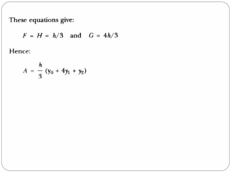
Simpson’s First Rule:

For many ship forms it is adequate to divide the length into ten

equal parts using eleven ordinates. When the ends have significant

curvature, greater accuracy can be obtained by introducing

intermediate ordinates in those areas, as shown in the following

Figure. This figure gives the Simpson multipliers to be used for

each consecutive area defined by three ordinates.

The total area is given by:

where y1, y3, y11 and y13 are the extra ordinates.

This method can be used to calculate any integral. Thus, it can be

applied to the first and second moments of area (used to find

centroids of areas).

These moments can be about the y-axis and x-axis that is the axis

through 0,

The moment of an area about an axis, is equal to the sum of all the

elements of the area times the distance of each element from the axis

about 0Y,

about 0X,

Y

X

y dx = element of area

The second moment of an area, known generally as the moment

of inertia of an area about an axis, is equal to the sum of all the

elements of the area times the square of the distance of each

element from the axis

Y

X

Example

Simpson’s Second Rule:

The area of a transverse section of a ship to successive waterlines may be

calculated and plotted in the form of a fair curve known as Bonjean curve.

The curves are often plotted on a profile of the ship like this:

Bonjean Curves

This enables the volume of displacement and centre of buoyancy to be

calculated at any waterline. These curves are particularly useful for

stability, strength, capacity and launching calculations.

From day to day a ship may be loaded to different drafts and different

trims. Therefore, underwater hull form characteristics over a range of

loading conditions need to be calculated. This is done by calculating each

characteristic at each loading condition (different waterlines).

The results of these calculations are plotted on closely spaced grid paper.

These curves are called hydrostatic curves or curves of form. The

following figure shows such a set. Vertical scale shows the ship’s draft.

Hydrostatic Curves

Displacement (salt water and fresh water)

VCB : vertical center of buoyancy

LCB : longitudinal center of buoyancy

LCF : longitudinal center of floatation

CB : block coefficient

CP : prismatic coeficient

CM : midship section coeficient

WS : wetted surface

KM : location of transverse metacentre above the baseline

MT1 : moment to trim one centimetre

Tons per one centimetre immersion

Sample hydrostatic curves

For the convenience of the deck officers, much of the numerical

information shown on the hydrostatic curves is repeated in the form

of tables, which most people find easier to use.

In cargo ships this information is incorporated in the capacity plan,

which also shows the volume of each hold and tank and its centre of

gravity. With that information at hand, the officers can predict the

ship’s drafts (fore and aft ) and stability characteristics for any

condition of loading.

Lets illustrate finding the area of the waterplane whose shape

is shown in the following Figure.

Example –Numerical area calculation for a waterline

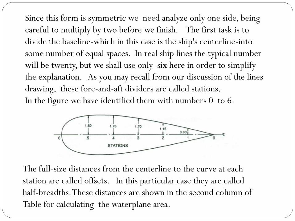
Since this form is symmetric we need analyze only one side, being

careful to multiply by two before we finish. The first task is to

divide the baseline-which in this case is the ship's centerline-into

some number of equal spaces. In real ship lines the typical number

will be twenty, but we shall use only six here in order to simplify

the explanation. As you may recall from our discussion of the lines

drawing, these fore-and-aft dividers are called stations.

In the figure we have identified them with numbers 0 to 6.

The full-size distances from the centerline to the curve at each

station are called offsets. In this particular case they are called

half-breadths. These distances are shown in the second column of

Table for calculating the waterplane area.

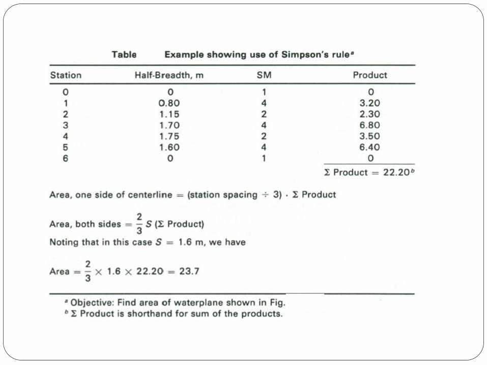
The third column in the table, identified as "SM," shows Simpson‘s

multipliers (the 1, 4, 2, 4 , etc.)

The final column shows the product of the half-breadth measurements

and Simpson's multipliers. The sum of all those products, when

multiplied by two-thirds the station spacing, will yield a close

approximation to the waterplane area-which is what we set out to find.

S is the station spacing

We have just explained how to apply the principles of numerical

analysis to approximate the area of a waterplane. Naval architects use

exactly the same procedure to find the area of any station below the

design waterline. That is, instead of analyzing a horizontal area they

analyze a vertical area (Bonjean curves).

They do this for several stations along the vessel's length. These cross-

sectional areas are then plotted to vertical scale against their fore-and-

aft locations, as shown in the following slide

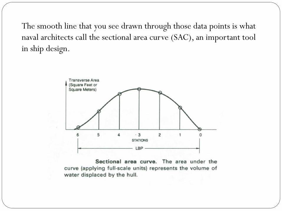
The smooth line that you see drawn through those data points is what

naval architects call the sectional area curve (SAC), an important tool

in ship design.

If we now apply Simpson's rule to this sectional area curve's offsets, we

can derive the ship's volume of displacement and its longitudinal center of

buoyancy.

In actual practice, what most naval architects often do is; they start by

drawing what they know to be a good sectional area curve and use that to

develop the individual stations, and then fair up the complete lines

drawing. This brings up the question of what is meant by

"a good sectional area curve"?

It is one that will provide the required displacement with a longitudinal

center of buoyancy that will lead to minimum wavemaking resistance.

In this lesson, an introduction to numerical analysis in naval architecture

has been introduced. It has been shown how areas and volumes, their

moments, enclosed by typical ship curves can be calculated by

approximate methods.