SEVENTH FRAMEWORK PROGRAMME THEME – ICT [Information and … · 2010-08-26 · sults available in...

SEVENTH FRAMEWORK PROGRAMMETHEME – ICT

[Information and Communication Technologies]

Contract Number: 223854Project Title: Hierarchical and Distributed Model Predictive Control of Large-

Scale SystemsProject Acronym: HD-MPC

HD−MPC

Deliverable Number: D5.1Deliverable Type: ReportContractual Date of Delivery: September 1, 2010Actual Date of Delivery: August 26, 2010Title of Deliverable: Report on the state of the art in dis-

tributed state and variance estimation,and on preliminary results on disturbancemodelling for distributed systems

Dissemination level: PublicWorkpackage contributing to the Deliverable: WP5WP Leader: Riccardo ScattoliniPartners: KUL, POLIMI, UNC, UWMAuthor(s): M. Farina, R. Scattolini, J. Garcia, J. Es-

pinosa, J.B. Rawlings

c© Copyright by the HD-MPC Consortium

HD-MPC ICT-223854 Distributed state and variance estimation

Table of contents

Executive Summary 3

1 Introduction to state estimation for distributed sensing architectures 6

2 Distributed state estimation 82.1 Statement of the problem . . . . . . . . . . . . . . . . . . . . . . . . . . . . . . . . 102.2 Information filter . . . . . . . . . . . . . . . . . . . . . . . . . . . . . . . . . . . . 102.3 Distributed Kalman filter based on consensus on measurements . . . . . . . .. . . . 112.4 Distributed Kalman filter based both on consensus on measurements and onconsensus

on estimates . . . . . . . . . . . . . . . . . . . . . . . . . . . . . . . . . . . . . . . 122.5 Distributed Kalman filter based on consensus on estimates with optimality properties 13

3 Partition-based state estimation 143.1 Statement of the problem . . . . . . . . . . . . . . . . . . . . . . . . . . . . . . . . 153.2 The distributed and decentralized Kalman filter . . . . . . . . . . . . . . . . . . .. 163.3 A consensus based overlapping decentralized estimator . . . . . . . . . .. . . . . . 17

4 Literature survey on variance estimation 184.1 Statement of the problem . . . . . . . . . . . . . . . . . . . . . . . . . . . . . . . . 19

4.1.1 Optimal case . . . . . . . . . . . . . . . . . . . . . . . . . . . . . . . . . . 204.1.2 Suboptimal case . . . . . . . . . . . . . . . . . . . . . . . . . . . . . . . . 20

4.2 Mehra’s algorithm . . . . . . . . . . . . . . . . . . . . . . . . . . . . . . . . . . . .214.3 Variance estimation with [40] . . . . . . . . . . . . . . . . . . . . . . . . . . . . . . 22

5 Preliminary results on disturbance modeling for distributed systems 255.1 Disturbance modeling in Model Predictive Control for offset-free tracking . . . . . . 255.2 Disturbance rejection and ISS stability in distributed control with MPC . . . . .. . 27

6 Conclusions 30

Bibliography 31

/35


Project co-ordinator

Name: Bart De SchutterAddress: Delft Center for Systems and Control

Delft University of TechnologyMekelweg 2, 2628 Delft, The Netherlands

Phone Number: +31-15-2785113Fax Number: +31-15-2786679

E-mail: [email protected]

Project web site: http://www.ict-hd-mpc.eu

/35

http://www.ict-hd-mpc.eu


Executive Summary

This report describes the research activity in the STREP research project Hierarchical and Dis-tributed Model Predictive Control of Large Scale Systems (HD-MPC), focusing on WP5 -“Distributed state estimation algorithms”. Specifically, the report aims at presenting the main re-sults available in the literature on the objects of Task 5.1 (State estimation) and Task 5.2 (Varianceestimation). The report also presents a concise review of the disturbancemodeling approachesused in Model Predictive Control to guarantee tracking properties or to achieve viability in frontof unknown inputs and modeling uncertainties. This analysis will be used to extend the main ideason disturbance modeling also to distributed systems, either to achieve tracking properties, or todesign distributed MPC algorithms with guaranteed stability.The report is organized in six chapters:

• Chapter 1 presents an introduction to the problem of distributed state estimation.A classifi-cation of the existing algorithms is proposed in terms of the topology of the communicationnetwork, of the amount of information transmitted among the processing units (agents) per-forming distributed estimation and, most importantly, of the specific problem considered. Inparticular, a distinction is made betweendistributed estimation, where each agent estimatesthe state of the whole system, andpartition-based estimation, where each agent estimatesonly part of the whole state based on its own measurements and on the information trans-mitted by its neighborhoods, including the estimates of other system’s components. Thisdistinction is not always clear in the technical literature, but it has a major impact on thealgorithms to be used in the two different problems.

• Chapter 2 is devoted to present the main algorithms available in the literature for distributedestimation. After an introductory example, the well-known observability property is conju-gated with the information available at any node (local observability, regional observability,i.e. the one based on the information directly collected by the agent and/or provided by itsneighborhoods, andcollective observability). A number of distributed algorithms based onthe Kalman filter and consensus algorithms are then described.

• Chapter 3 reviews the partition-based estimation algorithms proposed in the literature.Specifically, two algorithms, coping with overlapping partitions of large-scale systems,are described in detail; they are calleddistributed and decentralized Kalman filterandconsensus-based overlapping decentralized estimator. While for the former the commu-nication scheme is induced by the presence of overlapping states, for the latter the topologyof the network is defined by dependencies among the states of subsystems,resulting in aneighbor-to-neighbor communication scheme.

• The design of state estimators, based either on the Kalman filter or on the moving horizonapproach, require the knowledge, or a reliable estimate, of the noise covariance to computethe optimal estimator gain. This is a tight requirement, in particular for what concerns thedisturbance acting on the state variables, so that some approaches to variance estimationhave been proposed in the literature. In Chapter 4, these techniques arereviewed, focus-ing attention on two algorithms that appear to be the most reliable and efficient solutionsnowadays available to the considered problem.

/35


• Chapter 5 describes the main disturbance modeling assumptions used in ModelPredictiveControl (MPC) to achieve specific properties for the resulting closed-loop system. In par-ticular, in MPC disturbances are usually included in the problem formulation asconstantsignals to obtain feedback control laws guaranteeing asymptotic zero error regulation forconstant reference signals. Alternatively, the presence of bounded disturbances is consid-ered in the design of robust MPC laws leading to Input-to-State-Stable closed-loop systems.Both the cases are summarized in the chapter and their use in the design of distributed con-trol systems is discussed.

• Finally, in Chapter 6 some conclusions are drawn and some hints for future developmentson distributed state and variance estimation are reported.

/35


Chapter 1

Introduction to state estimation fordistributed sensing architectures

Recent advances in electronic devices with increasing computational power as well as in wirelesscommunication apparatuses allow for the development of sensor nodes with data processing and trans-mission capabilities characterized by low costs, low dimensions and low power consumption. As anexample, it is possible to mention the huge research efforts at the Universityof California, Berkeley’s,on the so-called smart dust, i.e. tiny wireless micro-electromechanical sensors which can transmitinformation like air quality-related measurements, temperature, humidity, light or vibrations, see forexample [68].

Given a large number of interconnected sensors, i.e. asensor network, a big challenge still widelyopen is to develop algorithms and protocols allowing the nodes of the network topossess self-organization capabilities and to operate cooperatively, so that each nodecan carry out local com-putations and transmit to the other nodes only the partially processed data required to achieve overallsensing objectives.

Therefore, the advantages and challenges of sensor networks are related to the possibility to buildlarge-scale networks, to implement sophisticated communication protocols, to reduce the amount ofcommunication required to perform tasks by distributed and/or local computations and, last but notleast, to implement complex power saving modes of operation. Among the many applications ofsensor networks, it is possible to recall the following:

• Health: sensor nodes can be deployed to monitor patients.

• Environmental monitoring: prevention of forest fires, forecast pollutant distribution over re-gions.

• Domotics: Improve quality and energy efficiency of environmental controls(air conditioning,ventilation systems, . . . ), while allowing reconfiguration and customization, besides savingwiring costs.

As also for the case of distributed control (see the survey paper [54]), to establish a taxonomycould be useful to cast different estimation algorithms, which will be presented in the following,into different classes. Different estimation methods can be classified according to the informationexchange between subsystems or nodes and according to the prior information that each sensor hasabout the process model.

/35


A first classification can be made depending on the topology of the communication network. Twocases can be identified:

• information is transmitted (and received) from any sensor node to all the other nodes (i.e.all-to-all communication);

• information is received by a given sensor nodei from a given subset of the othersVi , namelythe set ofi’s neighbors (neighbor-to-neighbor communication).

The exchange of information (also denoted data delivery) among nodes can be performed accord-ing to different protocols, which are presently under investigation (for an extensive review see [47]).In [65], sensor networks are classified as: continuous, event-driven and observer-initiated. In contin-uous models the nodes transmit information at a given transmission rate (whichcan be different fromthe observed process sampling frequency), in event-driven models thesensors transmit informationonly when a given event occurs, and in observer-initiated data models (also denoted request-replymodels) communications occur only in response to an explicit request (e.g. from the neighbors). Inthis work we focus on continuous data delivery models. Two main classes ofcontinuous data ex-change protocols can be identified, on the basis of the number of exchange events among subsystems.Namely:

• information is transmitted (and received) by the sensor nodes only once within each samplingtime (non-iterative algorithms);

• information can be transmitted (and received) by the local regulators many times (denotedNT)within the sampling time (iterative algorithms).

It is apparent that the amount of information available to the local regulatorswith iterative algorithmsis higher (for example, in the limit case whereNT → ∞, optimality of estimation algorithms can be,in general, guaranteed).

As also discussed in the survey paper [56], two main classes of estimation techniques for dis-tributed sensing schemes are presently under investigation. They are generally both referred, in theliterature, to asdistributed state-estimationalgorithms. For the sake of clarity and to avoid confusion,we now propose a new classification, adopted throughout the report, ofthese two problems.

• The first class of algorithms has the objective to make each node of the sensor network recoverthe estimate of the whole state vector. In this case, the solution relies on consensus (on mea-surements or on state estimates) and/or sensor-fusion algorithms. The main drawbacks of suchan approach are that each node should know the dynamic model of the overall observed sys-tem and that the estimation problem, solved by each sensor node, is a full order problem. Thisproblem will be denoteddistributed estimation.

• The second approach consists of estimating, for each node, a part of the global state-vector,using information transmitted by other sensors of the network. This problem, which will bedenotedpartition-based estimation, gives rise to low-order estimation problems solved in adecentralized way, and is particularly useful when the observed process is a large scale system.

Although they both aim at solving estimation problems for distributed sensing architectures, the math-ematical formulations of the two mentioned issues are deeply dissimilar, and their solutions requiredifferent mathematical methods. For these reason, they will be dealt with in different chapters (i.e.Chapter 2 and 3, respectively).

/35


Chapter 2

Distributed state estimation

As discussed in the previous chapter, many theoretical and technologicalchallenges have still to betackled in order to fully exploit the potentialities of sensor networks. As specified in the Introduction,one of the main issues is that of distributed state estimation, which can be described as follows.Assume that any sensors of the network measures some variables, computes a local estimate of theoverall state of the system under monitoring and transmits to its neighbors the measured values, thecomputed state estimation and the corresponding covariances. Then, the mainchallenge is to providea methodology which guarantees that all the sensors asymptotically reach a common reliable estimateof the state variables, i.e. the local estimates reach aconsensus. This goal must be achieved even ifthe measurements performed by any sensor are not sufficient to guarantee observability of the processstate (i.e.local observability), provided that all the sensors, if put together, guarantee such property(i.e. collective observability). The transmission of measurements and of estimates among the sensorsmust lead to the twofold advantage of enhancing the property of observability of the sensors and ofreducing the uncertainty of state estimates computed by each node.

Early works [21, 52] proposed distributed Kalman filters based on the parallelization of a central-ized Kalman filter which do not rely on consensus algorithms, but require all-to-all communication.Consensus algorithms for distributed state estimation based on Kalman filters have recently been pro-posed in [15, 4, 44, 41, 60, 42, 25]. In particular, in [44, 41, 60],consensus on measurementsis usedto reduce their uncertainty and Kalman filters are applied by each agent. In [42], three algorithmsfor distributed filtering are proposed. The first algorithm is similar to the one described in [41], savefor the fact that sensors exploit only partial measurements of the state vector. The second approachrelies on communicating the state estimates among neighboring agents (consensus on estimates). Thethird algorithm, namediterative Kalman consensus filter, is based on the discrete-time version of acontinuous-time Kalman filter plus aconsensus stepon the state estimates, which is proved to bestable. However, stability has not been proved for the discrete-time version of the algorithm and op-timality of the estimates has not been addressed. Recently, convergence in mean of the local stateestimates obtained with the algorithm presented in [41] has been proved in [25], provided that theobserved process is stable, and a stability analysis of the state estimator presented in [42] is providedin [43].In [4] consensus on the estimates is used together with Kalman filters. The weights of the sensors’estimates in the consensus step and the Kalman gain are optimized in order to minimize the estima-tion error covariance. A two-step procedure is also used in [15], where the considered observed signalis a random walk. A two-step algorithm is proposed, where filtering and consensus are performedsubsequently, and the estimation error is minimized with respect to both the observer gain and the

/35


consensus weights. This guarantees optimality of the solution.Some of the methods mentioned above have been reviewed and compared in [56].

More in general, the issue of distributed sensor fusion has been widely studied in the past years,see e.g. [13, 61]. The paper [13] provides an algorithm accounting for dynamically changing inter-connections among sensors, unreliable communication links, and faults, where convergence of theestimates to the true values is proved, under suitable hypothesis of “dynamical” graph connectivity,while in [61] the authors propose a minimum variance estimator for distributed tracking of a noisytime-varying signal.

As a simple example of a distributed state estimation problem, taken from [15], assume to haveMsensors measuring the same temperatureT, whose dynamic evolution is

Tk+1 = Tk+wk (2.1)

wherew is a white noise, any sensori, i = 1, ...,M provides the measurement

yik = Tk+vi

k (2.2)

and thevi ’s are white noises with the same variance.In order to obtain a more reliable estimate ofT, adata fusionalgorithm is required. This can triviallyrely on a centralized estimator placed in abase stationcomputing the estimate

Tk+1 = Tk+L(yk− Tk) (2.3)

whereL is a gain to be suitably selected and

yk =1M ∑

i=1,...,M

yik (2.4)

Alternatively, the sensors can be arranged in a communication graph configuration. Their mea-surements are not sent simultaneously and instantaneously to the base station; rather, each sensorcomputes a local estimationT i

k based on its available information, i.e. its local measurements, and theinformation provided by its neighborhoods. In this case, a suitable local estimator can be describedby

T ik+1 = m(Tk)

i +L(m(yk)i −m(Tk)

i) (2.5)

wherem(Tk)i and m(yk)

i representmean(to be specified) values of estimates and measurements,respectively, and are computed on the basis of the information exchangedby sensori with its neigh-borhoods. In this case, it is possible to say that the estimateT i depends onregional quantities, i.e.on quantities available to sensori through its sensing capabilities and through the nodes linked toit. The termsm(Tk)

i andm(yk)i are then average values computed from the regional quantities by

means ofconsensus. Increasing the number of transmissionsNT among neighboring sensors withinone sampling time, it is possible to obtain that

m(yk)i → yk (2.6)

so that, even ifm(Tk)i = T i

k , the local filters become “optimal”, with the performance of the centralizedfilter. In view of these considerations, it is apparent that consensus is crucial to achieve an agreementamong local variables, and it is the milestone of the distributed estimation algorithms proposed sofar in the literature. In fact, all the methods available basically rely onconsensus on measurements,consensus on estimatesor on both of them.

In the following, some prototype algorithms will be briefly presented to illustrate the main char-acteristics of the different approaches. First of all, a formal statement of the problem will be given,and the classical (centralized) Kalman filter will be recalled in itsinformation form.

/35


2.1 Statement of the problem

In order to state the distributed estimation problem more formally and in general terms, assume thatthe measured system evolves according to the linear dynamics

xt+1 = Axt +wt (2.7)

where the statex and the disturbancew are constrained as follows:x∈ X⊆ Rn, w∈W⊆ R

n, whereX andW are closed and compact sets. The initial statex0 is a random variable with meanµ andcovarianceΠ0, while the covariance ofw is denoted byQ. The system is assumed to be sensed byMnodes, with sensing models

yit =Cixt +vi

t , i = 1, · · · ,M (2.8)

wherevi is a white noise with covarianceRi ∈ Rpi×pi .

The communication network is described by a directed graphG = (V ,E ) whereV is the set ofvertices andE ∈ V ×V is the set of edges. Moreover,V k

i is the set of verticesν j such that thereexists a path of length at mostk from ν j to νi . Finally, associated to the graphG it is possible to definea matrixK compatible with the graph itself, whose elements(i, j) are such thatki j ≥ 0 if (i, j) ∈ E ,ki j = 0 otherwise, and∑M

j=1ki j = 1 for all i = 1, . . .M. Given a graph topology, the freedom allowedin the choice of the elementski j can be fruitfully exploited to enhance the performance of the adoptedconsensus algorithms. MatrixK is often used in consensus algorithms to perform averaging on themeasurements or on the estimates.Finally, it is useful to distinguish betweenlocal, regionalandcollectivequantities. Specifically, forthe nodei, the quantityz will be denoted:

• local (indicated withzi), if related to nodei solely;

• regional (indicated withzi), if referred toVNT

i ;

• collective (indicated withz), if referred to the whole network.

Accordingly, given the measurementsyi , yi andy, it is possible to trivially define the output transfor-mation matricesCi (local output transformation, see (2.8)),C

i(regional output transformation) andC

(collective output transformation). Then, it will be said that the system is

• locally observable by nodei if the pair(A,Ci) is observable;

• regionally observable by nodei if the pair(A,Ci) is observable;

• collectively observable if the pair(A,C) is observable.

2.2 Information filter

Consider the linear system with its (collective) output described by

xt+1 = Axt +wt

yt = Cxt +vt

Let xk1/k2= E[xk1/y1, . . . ,yk2] be the expected value ofxk1 given the outputs up to timek2, denote

by Πk1/k2= E

[(xk1 − xk1/k2

)(xk1 − xk1/k2)T]

its covariance and defineR = diag(R1, . . . ,RM). Then, the

/35


information filter evolves according to the following steps:

Predictor step

Πk/k−1 = AΠk−1/k−1AT +Q

xk/k−1 = Axk−1/k−1

Corrector step

Πk/k = (Π−1k/k−1+F)−1

xk/k = Πk/k(Π−1k/k−1xk/k−1+ fk)

where

F = CTR−1C =M

∑i=1

CiT (Ri)−1Ci

fk = CTR−1yk =M

∑i=1

CiT (Ri)−1yik

Note that the predictor step can be performedlocally by the M sensors, while the corrector steprequires thecollective datavectory.

2.3 Distributed Kalman filter based on consensus on measurements

Starting from the centralized form of the Information Filter, in [44, 41, 60, 25] a distributed implemen-tation has been proposed, relying on transmission and consensus operations on measurements solely.In particular, letting ˆxi

k1/k2be the estimate ofxk1 carried out by sensori at instantk2, and denoting by

Πik1/k2

= E[(xk1 − xi

k1/k2)(xk1 − xi

k1/k2)T]

its covariance, the prediction and correction steps are modi-

fied as follows:

Predictor step

Πik/k−1 = AΠi

k−1/k−1AT +Q

xik/k−1 = Axi

k−1/k−1

Corrector step

Πik/k = ((Πi

k/k−1)−1+ F i)−1

xik/k = Πi

k/k((Πik/k−1)

−1xik/k−1+ f i

k)

where F i is the local estimate ofF = ∑Mi=1CiT (Ri)−1Ci and f i

k is the local estimate offk = ∑M

i=1CiT (Ri)−1yik. These local estimates can be obtained with consensus filters on the basis

of regional measurements. However, if regional observability does nothold, the algorithm can notgive reliable results; although, for specific topologies of graphs, the distributed estimation algorithmcan be considered as a good approximation of the centralized Information Filter for a large numberof intercommunications between successive sampling times (NT ≫ 1). A stronger results has been

/35


reported in [25], where it has been proved that for asymptotically stable systems, the local state esti-mates produced by the distributed algorithm converge in the mean to the centralized state estimate. A“smarter” way to use the propagation of information through the network hasbeen discussed in [4],where the exploited rationale is to take advantage of the delayed information passing from one nodeto another even whenNT = 1. This can be easily obtained by considering an augmented system wherethe current state is considered together with its past values over a window of suitable length.

2.4 Distributed Kalman filter based both on consensus on measure-ments and on consensus on estimates

An evolution of the previous distributed Kalman filters has been described in [42], where transmissionof both the local measurements and the local estimates is used to achieve consensus. The algorithmevolves according to the following steps:

Predictor step

Πik/k−1 = AΠi

k−1/k−1AT +Q

xik/k−1 = Axi

k−1/k−1 (2.9a)

Consensus on measurements

F i = ∑j∈V i

C j T (Rj)−1C j

f ik = ∑

j∈V i

C j T (Rj)−1y jk (2.9b)

Corrector step+consensus on estimates

Πik/k = ((Πi

k/k−1)−1+ F i)−1

xik/k = Πi

k/k((Πik/k−1)

−1xik/k−1+ f i

k)+K icons ∑

j∈V i

(x jk/k−1− xi

k/k−1)

= xik/k−1+Πi

k/k( f ik− F i xi

k/k−1)+K icons ∑

j∈V i

(x jk/k−1− xi

k/k−1) (2.9c)

whereK icons is the consensus on estimates gain. With respect to the above algorithm, two remarks are

in order. First, in [42] it has been proved that it is possible to achieve convergence of the estimatesfor an analogous algorithm developed in continuous time and under the main assumption of collec-tive observability, but no theoretical results are given for the discrete timeimplementation previouslydescribed. Second, as discussed in [15], the algorithm does not guarantee optimality, since in case ofdistributed algorithms the optimal gain does not coincide with the Kalman gain.These issues have been explored in a recent contribution [43], wherea formal stability proof is givenand performance analysis of the algorithm are provided. Specifically, in [43], the algorithm (2.9) is de-noted Kalman Consensus Information Filter if the consensus on measurementstep (2.9b) is performed,and it is called Kalman Consensus Filter if consensus on measurement (2.9b)is not performed (i.e. ifF i = CiT (Ri)−1Ci and if f i

k = CiT (Ri)−1yik). For the Kalman Consensus Filter, for a specific choice

of the consensus gainK icons, under the assumption that the information matrix(Ci)TRiCi is positive

definite for all i andk ≥ 0, the error dynamics of the Kalman-Consensus filter is globally asymp-totically stable. Furthermore, all estimators asymptotically reach a consensus on state estimates, i.e.x1

k = · · ·= xMk for k→ ∞.

/35


2.5 Distributed Kalman filter based on consensus on estimates with op-timality properties

As discussed in [4, 5, 6], to guarantee optimality of the distributed Kalman filter,the Kalman gainand the weights on the sensors’ estimates (i.e. the elementski j of the graph matrixK introduced inthe previous Chapter) should be the result of an optimization. For instance,the following algorithm isproposed in [4]:

Local information update

xi,localk/k = xi,reg

k/k−1+Gi(yik−Ci xi,reg

k/k−1)

Regional consensus on the estimates

xi,regk/k = ∑

j∈V i

ki j xi,localk/k

Prediction

xi,regk+1/k = Axi,reg

k/k

In this algorithm, the gainsGi and the matrixK = ki j must be determined to minimize the steadystate estimation error covariance matrices. Unfortunately, this minimization problem is not convex,while some bootstrap (iterative 2-step) algorithms have been proposed in [4]. In [5], an evaluation ofthe performance of such algorithm applied to an ultrasound based positioning application with sevensensor nodes is provided. In [6], the weight selection process has been analyzed yielding performanceimprovements for some studied examples, and solutions to both optimization problemsinvolved inthe iterative off-line weight selection process are given in terms of closedform expressions. Theconvergence properties of the presented method are still an open problem.

/35


Chapter 3

Partition-based state estimation

Partition-based state-estimation algorithms for large-scale systems decomposed into physically cou-pled subsystems is of paramount importance in many engineering control problems, such as powernetworks [57], transport networks [53], process control [66] and robotics [38]. Starting from theidea to decompose a large-scale problems into small-scale ones in order to handle complexity, highcomputer memory and computational load involved in the solution of centralized state-estimationproblems, many studies focused on the design of partition-based filters. The different solutions pro-posed can be classified according to the model used by each subsystem for state-estimation purposesand to the topology of the communication network among subsystems. Besides thecomputationalbenefits of such an approach, in [58] it is highlighted that decomposition can provide insight aboutthe structural properties of dynamical systems, i.e. robustness of stability,optimality, controllabilityand observability to structural perturbations and to uncertainties (e.g. on the models of the subsystemsand on the connections between them). Recently, there has been a revival of interest on these issues,leading to the plug-and-play paradigm [64].

For large scale continuous-time systems, decentralized estimation schemes have been proposedin [58] and [1], where stability conditions for the design of decentralized observers are establishedusing the theory developed in the framework of decentralized control in [57].The estimation problem for large-scale systems in the discrete-time framework has received moreattention, during the years. In [22] a two-level decentralized computational structure is developed,applied to a large-scale system consisting inM dynamically coupled subsystems with uncoupled mea-surements. The method proposed in that paper provides optimal estimation andis designed in such away that each subsystem performs low-order computations. The main drawback is that the algorithmrequires all-to-all communication and it is iterative.Later work aimed at reducing the computational complexity of centralized Kalmanfiltering by paral-lelizing computations [21, 52]. The algorithm proposed in [21] assumes local processing capabilitiesfor each subsystem, but relies on a central processing unit for globaldata fusion. On the other hand,the algorithm proposed in [52] does not require a base processing station for global data fusion. There-fore it is denoted in [52] asfully decentralized. However, since both [21] and [52] require all-to-allcommunication and assume each subsystem has full knowledge of the whole dynamics, they shouldbe considered as distributed estimation algorithms rather than partition-based ones.Starting from the idea of model distribution and of local (nodal) models [10],in [37] the focus is onthe use of reduced-order and decoupled models for each subsystem. The proposed solutions, besideneglecting coupling, exploit communication networks that are almost fully connected. Subsystemswith overlapping states have been considered in [27, 62, 66, 67]. While inthe estimation schemes in

/35


[66, 67] the communication scheme is induced by the presence of overlapping states (which, in princi-ple, can lead to an all-to-all communication scheme), in [27, 62] the topology ofthe network is definedby dependencies among the states of subsystems resulting in a neighbor-to-neighbor communicationscheme.

In the following, some partition-based algorithms will be presented. First, a general statement of theproblem (in the linear framework) is given.


Consider the autonomous discrete-time linear system

xt+1 = Axt +wt , (3.1)

wherext ∈ Rn is the state vector, whilewt represents a disturbance with varianceQ > 0. The initial

conditionx0 is a random variable with meanmx0 and covariance matrixΠΠΠ0 > 0. Measurements onthe state vector are performed according to the sensing model

yt = Cxt +vt (3.2)

wherevt ∈ Rp is a white noise with varianceR > 0.

Let system (3.1) be partitioned inM low order interconnected submodels, i.e. where a genericsubmodel hasx[i]t ∈ R

ni as state vector. We say that the subsystems states are overlapping if there isat least a component ofxt which is part of the state vector of more than one subsystem. Otherwise,we say that the subsystems states are non-overlapping. We can denote, for all i = 1, . . . ,M, x[i]t = Tixt ,whereTi is a linear nodal transformation matrix.Accordingly, the state transition matricesA[1] ∈ R

n1×n1, . . . , A[M] ∈ RnM×nM of theM subsystems are

given byA[i] =TiAT†i , where † denotes the generalized inverse. In general,Ti is assumed for simplicity

to be a scaled orthonormal transformation. Note that, in general,∑Mi=1ni ≥ n, where the equality holds

only if the states of the subsystems are non-overlapping.The i-th subsystem obeys to the linear dynamics

x[i]t+1 = A[i] x[i]t +u[i],xt +w[i]t , (3.3)

wherex[i]t is the state vector,u[i],xt collects the effect of state variables of other subsystems, and thetermw[i]

t is a disturbance with varianceQ[i]. The initial conditionx[i]0 is a random variable with mean

m[i]x0 and covariance matrixΠ[i]

0 . Note thatQ[i] > 0, R[i] > 0 andΠ[i]0 > 0 can be obtained fromQ, R and

ΠΠΠ0. For example, in [62],Q[i], R[i] andΠ[i]0 are diagonal blocks ofQ, R andΠΠΠ0 of appropriate size.

According to (3.2) and to the state partition, the outputs of the subsystems are given by

y[i]t =C[i] x[i]t +u[i],yt +v[i]t (3.4)

whereu[i],yt collects the effect of the state variables of other subsystems, and the termv[i]t ∈ Rpi repre-

sents white noise with variance equal toR[i].We denote with ˆx[i]t1/t2

the estimate ofx[i]t1 performed at timet2 by subsystemi. Its error covariance

matrix is denoted withΠ[i]t1/t2

/35


Remark In general, some outputs of system (3.1) can be considered as outputs ofmore than onesubsystem, i.e. ¯p= ∑m

i=1 pi ≥ p. Notice, however, that in decentralized control, each local subsystemcommonly uses local information, which reduces the amount of transmitted information betweensubsystems.

The system partition induces an interconnected network of subsystems, which can be described bya directed graphG = (V ,E ), where the nodes inV are the subsystems and the edge( j, i) in theset E ⊆ V × V models that thej-th subsystem influences the dynamics or the output of thei-thsubsystem.

3.2 The distributed and decentralized Kalman filter

In [66, 67] and algorithm denoted distributed and decentralized Kalman filter(DDKF) is presented,designed for overlapping partitions. Furthermore, one of the main contributions of [66] is an intriguingdiscussion on sampling and partitioning of large-scale systems. For instance, the authors point outthat the main issues involved in partitioning of the overall system into subsystemsare(i) similarityof the subsystems network to the actual plant,(ii) the computational load at each subsystem,(iii ) thecommunication burden and(iv) the available computational resources. They also point out that thereis a trade-off between(ii) and(iii ) and they propose an heuristic procedure for partitioning.As far as the DDKF algorithm is concerned, it neglects the dynamic and the output coupling terms(denotedu[i],xt andu[i],yt in (3.3) and in (3.4), respectively), and it is composed in two steps:

• Prediction step: for all i = 1, . . . ,M

x[i]t+1/t = A[i]x[i]t/t (3.5)

Π[i]t+1/t = A[i]Π[i]

t/t(A[i])+Q[i] (3.6)

• Estimation step: for all i = 1, . . . ,M

x[i]t/t = Π[i]t/t

[(Π[i]

t/t−1)−1x[i]t/t−1+

M

∑j=1

(Π[i j ]t/t )

†x[i j ]t/t

](3.7)

Π[i]t/t =

[(Π[i]

t/t−1)−1+

M

∑j=1

(Π[i j ]t/t )

†

]−1

(3.8)

where, for subsystemi, x[i j ]t/t andΠ[i j ]t/t are the estimate and the covariance matrix related to the

measurementy[ j]t , for j = 1, . . . ,M, and they are defined as follows

x[i j ]t/t = TiT†j ((C

[ j])T(R[ j])†C[ j])†(C[ j])T(R[ j])†y[ j]t (3.9)

Π[i j ]t/t = Ti

[TT

j ((C[ j])T(R[ j])†C[ j])Tj

]†TT

i (3.10)

Notice that, forj 6= i, the transmissions between subsystemj to subsystemi must be performedonly if subsystemsi and j have overlapping state variables (i.e.TiT

†j 6= 0). Otherwise, ifTiT

†j =

0 identically, we have that ˜x[i j ]t/t = 0 andΠ[i j ]t/t = 0 and therefore such terms do not appear in

equations (3.7) and (3.8).

/35


3.3 A consensus based overlapping decentralized estimator

In [62, 63] an algorithm is proposed, which combines local Kalman-type estimators with a dynamicconsensus strategy. While [63] deals with continuous-time systems, [62] encompasses the case ofdiscrete-time systems.Assuming that the pairs(A[i],C[i]) are detectable and that the pairs(A[i],(Q[i])

12 ) are stabilizable for all

i = 1, . . . ,M, the proposed method is composed by two steps: a local Kalman filter step and acon-sensus one. While the former involves low-order computations, the consensus step requires that eachnode computes and stores an estimate of the large-scale-scale system statext . Importantly however,each node does not need to have knowledge about the whole system dynamics (3.1).We definex[i]t1/t2

as the estimate of the overall system statext1 performed by thei-th subsystem at timet2.

To perform a local Kalman filter, for alli = 1, . . . ,M the local estimator is updated according tothe equation

x[i]t+1/t = A[i](

x[i]t/t−1+ γi(t)L[i][y[i]t −C[i]x[i]t/t−1

])(3.11)

whereL[i] is the steady-state Kalman gain given by

L[i] = Π[i](C[i])T[C[i]Π[i](C[i])T +R[i]

]−1

Π[i] is a solution of the algebraic Riccati equation

Π[i] = A[i][Π[i]−L[i]C[i]Π[i]

](A[i])T +Q[i]

andγi(t) = 1 when thei-th agent receives measurementsy[i]t , and 0 otherwise (in order to account formissing observations).

The large-scale system state estimator performed by each agent requiresthe definition of a numberof matrices on the basis of the local-system matrices:A[i] ∈R

n×n has at mostni ×ni nonzero elementsequivalent to those ofA[i], placed at suitable positions, i.e. beingx[i]t = Tixt , then A[i] = T†

i A[i]Ti .MatricesC[i] andL [i] are pi × n andn× pi matrices, respectively, obtained fromC[i] andL[i] in thesame way asA[i] is obtained fromA[i]. From (3.11), the consensus-based Kalman-like estimatorequations, fori = 1, . . . ,M, are

x[i]t/t = x[i]t/t−1+ γi(t)L [i][y[i]t −C[i]x[i]t/t−1

](3.12)

x[i]t+1/t =M

∑j=1

Ci j (t)F[ j]x[ j]t/t (3.13)

whereCi j (t) ∈ Rn×n, i, j = 1, . . . ,M are time varying gain matrices such thatCi j (t) = 0 if no commu-

nication between nodej and i is allowed (i.e. if( j, i) 6 ∈E ). Otherwise,Ci j (t) are diagonal matriceswith nonnegative entries. The termsCi j (t) are block elements of a consensus matrixC(t) = Ci j (t),which must be row-stochastic, and it is compatible with the communication graphG by definition ofCi j (t), for all i, j = 1, . . . ,M.

Stability conditions for the collective estimation error dynamicsεεε t = (x[1]t/t −xt , . . . , x[M]t/t −xt) are pro-

vided in [62], where an optimal procedure for choosing the matricesCi j (t) is also proposed.

/35


Chapter 4

Literature survey on variance estimation

Model-based control methods, such as model predictive control (MPC), have become popular choicesfor solving difficult control problems. Higher performance, however,comes at a cost of greater re-quired knowledge about the process being controlled. Expert knowledge is often required to properlycommission and maintain the regulator, to compute target calculation, and to develop state estimatorsof MPC, for example. This chapter addresses the required knowledge for the project of the state es-timator, and describes some techniques with which ordinary closed-loop datamay be used to removesome of the information burden from the user. Consider the usual linear, time-invariant, discrete-timemodel

x(k+1) = Φx(k)+Γu(k)+w(k)

y(k) = Hx(k)+e(k)

in which Φ ∈ Rn×n, Γ ∈ R

n×m, H ∈ Rp×n, andw(k) ande(k) are uncorrelated zero-mean Gaussian

noise sequences with covariancesQ andR, respectively. The sequenceu(k) is assumed to be a knowninput. State estimates of the system are considered using a linear, time-invariant state estimator

x(k+1/k) = Φx(k/k)+Γu(k)

x(k/k) = x(k/k−1)+L[y(k)−Hx(k/k−1)]

in which L is the estimator gain, not necessarily optimal. We denote the residuals of the output equa-tions (y(k)−Hx(k/k−1)) as theL-innovations when calculated using a state estimator with gainL.In order to use the optimal filter, we need to know the covariances of the disturbances,Q,R fromwhich we can calculate the optimal estimator’s error covariance and the optimalKalman filter gain.In most industrial process control applications, however, the covariances of the disturbances enteringthe process are not known. To address this requirement, estimation of the covariances from open-loopdata has long been a subject in the field of adaptive filtering, and can be divided into four generalcategories: Bayesian [7, 23], maximum likelihood [11, 26], covariance matching [39], and corre-lation techniques. Bayesian and maximum likelihood methods have fallen out of favor because oftheir sometimes excessive computation times. They may be well suited to a multi-model approachas in [8]. Covariance matching is the computation of the covariances from theresiduals of the stateestimation problem. Covariance matching techniques have been shown to givebiased estimates of thetrue covariances. The fourth category is correlation techniques, largely pioneered by Mehra [34, 35]and Carew and Belanger [9, 14]. In [40] an alternative method to the one presented in [34, 35] isdescribed, where necessary and sufficient conditions for uniqueness of the estimated covariances are

/35


also given. In [40] an exhaustive comparison with the method proposed in[34] is provided, showingcases where the latter is outperformed by the algorithm proposed in [40].In [3] an algorithm is presented, following the analysis from [40] and generalized in [2] for systemswith correlated process and measurement noises. Two contributions can be highlighted: the general-ization of the autocovariance least-square method to systems with correlated noise, and the interior-point predictor-corrector algorithm for solving the symmetric semidefinite least-squares problem.In Section 4.1 the problem of covariance estimation is formally stated, while in Sections 4.2 and 4.3the algorithms presented in [34] and in [40], respectively, are reviewedin details.


Let us consider the process described by the autonomous system:

x(k+1) = Φx(k)+w(k)y(k) = H x(k)+e(k)

(4.1)

wherex,w∈ Rn, y,e∈ R

p, andΦ ∈ Rn×n andH ∈ R

p×n.In general the stochastic processesw ande are considered to be independent and uncorrelated whitenoises with zero mean and covariance matrices:

E[w(k)w(k)T]= Q0 (4.2a)

E[e(k)e(k)T]= R0 (4.2b)

We consider these matrices to be not known a priori, while ana priori assumption is made on thestructure ofQ0 (i.e. position of the zero entries). For instance, we assume thatQ0 hasm≤ n unknownparameters. For notation purposes, we denote:

. x(k1/k2) is the estimate ofx(k1) based on all the measurements up tok2, i.e.y(1), . . . ,y(k2);

. ε(k) = x(k)− x(k/k−1) indicates the 1-step state prediction error;

. v(k) = y(k)−Hx(k/k−1) is the innovation;

. Q andR the estimates ofQ0 andR0;

. Πk = E[ε(k)ε(k)T

]the covariance matrix of the prediction error;

. V ik = E

[v(k)v(k− i)T

]the covariance function of the innovation. For simplicity we indicate

V0k =Vk.

Let us consider the classical structure of the Kalman filter

x(k+1/k) = Φx(k/k)x(k/k) = x(k/k−1)+Lo

k(y(k)−Hx(k/k−1))(4.3)

whereLok is the Kalman gain, whose expression will be computed in the following, in orderto mini-

mize the prediction error covariance.

/35


4.1.1 Optimal case

Let’s fist consider the case where the noise covariance matrices are exactly knowna priori, namelywhere, lettingR andQ the estimates used in the filter design

R= R0 (4.4a)

Q= Q0 (4.4b)

We can compute

ε(k+1) = Φ(I −Lok H)ε(k)−ΦLo

k e(k)+w(k) (4.5)

ThereforeΠk+1 = Φ

(I −Lo

k H)

Πk(I −Lo

k H)T ΦT +ΦLo

k R0(Lok)

TΦT +Q0

= ΦΠk ΦT +Q0+ΦLok (H Πk HT +R0)(Lo

k)TΦT+

−ΦLok H Πk ΦT −ΦΠk HT (Lo

k)TΦT

(4.6)

Let us define

SST = (H Πk HT +R0) (4.7)

Therefore we obtain that

Πk+1 = ΦΠk ΦT +Q0+Φ(Lok S−A)(Lo

k S−A)TΦT −ΦAATΦ (4.8)

whereA= ΦΠk HT (ST)−1. Minimizing Πk+1 with respect to the gainLok we obtain:

minLo

k

Πk+1 = ΦΠk ΦT +Q0−ΦΠk HT (H Πk HT +R0)−1H Πk ΦT (4.9)

with optimal gain:Lo

k = AS−1 = Πk HT (H Πk HT +R0)−1 (4.10)

4.1.2 Suboptimal case

Thesuboptimal casecorresponds to the case where uncertain values of the variance matricesR0 andQ0 are given, i.e.

R 6= R0

Q 6= Q0

In this case we might introduce two new variablesΠk andΠk. We denote asΠk the real valueassumed by the covariance matrix of the estimation error, i.e.

Πk = E[ε(k)ε(k)T] (4.11)

while Πk represents the estimated value of such matrix, given in (4.6), where, instead of R0 andQ0,we use the valuesR andQ. We have that

Πk+1 = Φ(I −Lok H) Πk (I −Lo

k H)T ΦT +ΦLok R0(Lo

k)TΦT +Q0 (4.12a)

Πk+1 = Φ(I −Lok H) Πk (I −Lo

k H)T ΦT +ΦLok R(Lo

k)TΦT + Q (4.12b)

We can easily see from the previous equations that, whileLok in (4.10) minimizesΠk, the real covari-

ance of the estimation errorΠk is not minimized by formula (4.10). Furthermore it is also possible toinfer thatv(k) is a white noise process only in the optimal case (see the next Section 4.2).

/35


4.2 Mehra’s algorithm

In [34] a method is proposed, for the unbiased estimation ofQ0 andR0, based on the analysis ofv(k) given by the application of a suboptimal Kalman filter. The main steps of the algorithm are thefollowing

(i) application of (4.10) (steady state formulation);

(ii) test of optimality of the Kalman filter applied at step(i);

(iii ) in case the optimality test fails, new estimates of matricesQ0 andR0 are computed.

The optimality test at step(ii) consists in verifying that the innovation sequencev(t) is white. Fordetails see [34]. In the next section a sketch of the algorithm proposed for the estimation ofQ0 andR0 is provided. The author relies on two main assumptions:(I) the pair(Φ,H) is observable and(II )the transition matrixΦ is non-singular.From now on the steady-state formulation of the Kalman filter is applied. Therefore,V i , Π andLo

denote the asymptotic values ofV ik, Πk andLo

k, respectively. Similarly,Π andΠ denote the asymptoticvalues ofΠk andΠk, respectively. Specifically,Π is the result of the algebraic Riccati equation

Π = Φ(I −LoH)Π(I −LoH)TΦT +ΦLoR(Lo)TΦT + Q (4.13)

whereLo = ΠHT (H ΠHT + R)−1

while Π is the result of the equation

Π = Φ(I −LoH)Π(I −LoH)TΦT +ΦLoR0(Lo)TΦT +Q0 (4.14)

Schematically, the proposed method for variance estimation can be sketched as follows.

1) We will denote asV i the sampled estimate ofV i , which can be computed, for example, accord-ing to the following equation

V i =1

Ndata

Ndata−i

∑k=1

v(k)v(k+ i)T

whereNdata denotes the available number of data samples.

2) It can be shown that, in steady state,v(k) has variance equal to

V =V0 = H ΠHT +R0 (4.15)

and covarianceV i , for i ≥ 1:

V i = H [Φ (I −LoH)]i−1 Φ[ΠHT −LoV0] (4.16)

Rewriting (4.16), and replacingV i with its sampling counterpartV i , for all i = 0, . . . ,k, weobtain that

V1 = HΦΠHT −HΦLoV0

V2 = HΦ2ΠHT −HΦLoV1−HΦ2LoV0

...Vk = HΦkΠHT −HΦLoVk−1−·· ·−HΦkLoV0

/35


Therefore, one obtains that an estimateˆΠHT of ΠHT can be computed as

ˆΠHT = B†

V1+HΦLoV0

V2+HΦLoV1+HΦ2LoV0

...Vk+HΦLoVk−1+ · · ·+HΦkLoV0

(4.17)

whereB† denotes the pseudo-inverse ofB, which is defined as

B=

HHΦ

...HΦk−1

Φ

Under the observability assumption, and if the transition matrixΦ is non-singular, ifk is greaterthan the observability index of the pair(Φ,H), then the pseudo-inverse ofB can be computed.

3) Compute a new estimateR of R0 according to the equation (4.15), i.e.ˆR= V0−H( ˆΠHT)

4) Compute an estimate ofQ0 using the equation (4.14). One can write, from (4.14), that

Π = Q0+ΦΠΦT +Ω (4.18)

whereΩ = Φ [−LoHΠ− ΠHT(Lo)T +LoV0(Lo)T ]ΦT (4.19)

an estimate of which can be computed based on the previous steps. Iterating (4.18) one obtainsthat, for allk> 1

Π = ΦkΠ(Φk)T +k−1

∑j=0

Φ jΩ(Φ j)T +k−1

∑j=0

Φ jQ0(Φ j)T (4.20)

Pre-multiplying both sides of equation (4.20) byH and post-multiplying it by(Φ−k)THT oneobtains that, fork≥ 1

k−1

∑j=0

HΦ jQ0(Φ j−k)THT = HΠ(Φ−k)THT −HΦkΠHT −k−1

∑j=0

HΦ jΩ(Φ j−k)THT (4.21)

Note that an estimate of the right hand side of equation (4.21) is given, sinceV0 and ˆΠHT havebeen previously computed. After choosing a linearly independent set ofequations (4.21) (fordetails see [34]), one can identify them≤ n unknown entries ofQ0.

4.3 Variance estimation with [40]

Consider a linear, time-invariant, discrete-time autonomous model (4.1). State estimates of the systemare considered using a linear, time-invariant state estimator with observer gain L

x(k+1|k) = Φx(k|k)

x(k|k) = x(k|k−1)+L [y(k)−Hx(k|k−1)](4.22)

/35


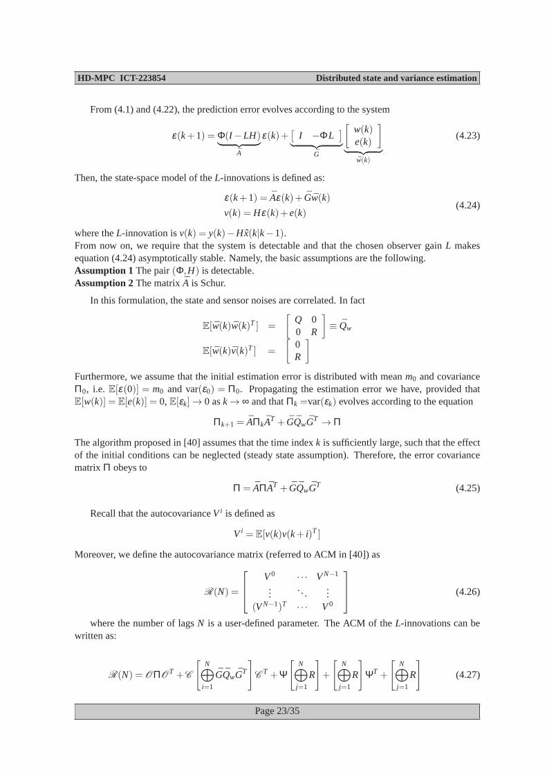
From (4.1) and (4.22), the prediction error evolves according to the system

ε(k+1) = Φ(I −LH)︸︷︷︸A

ε(k)+[

I −ΦL]

︸︷︷︸G

[w(k)e(k)

]

︸︷︷︸w(k)

(4.23)

Then, the state-space model of theL-innovations is defined as:

ε(k+1) = Aε(k)+ Gw(k)

v(k) = Hε(k)+e(k)(4.24)

where theL-innovation isv(k) = y(k)−Hx(k|k−1).From now on, we require that the system is detectable and that the chosen observer gainL makesequation (4.24) asymptotically stable. Namely, the basic assumptions are the following.Assumption 1The pair(Φ,H) is detectable.Assumption 2The matrixA is Schur.

In this formulation, the state and sensor noises are correlated. In fact

E[w(k)w(k)T ] =

[Q 00 R

]≡ Qw

E[w(k)v(k)T ] =

[0R

]

Furthermore, we assume that the initial estimation error is distributed with meanm0 and covarianceΠ0, i.e. E[ε(0)] = m0 and var(ε0) = Π0. Propagating the estimation error we have, provided thatE[w(k)] = E[e(k)] = 0,E[εk]→ 0 ask→ ∞ and thatΠk =var(εk) evolves according to the equation

Πk+1 = AΠkAT + GQwGT → Π

The algorithm proposed in [40] assumes that the time indexk is sufficiently large, such that the effectof the initial conditions can be neglected (steady state assumption). Therefore, the error covariancematrix Π obeys to

Π = AΠAT + GQwGT (4.25)

Recall that the autocovarianceV i is defined as

V i = E[v(k)v(k+ i)T ]

Moreover, we define the autocovariance matrix (referred to ACM in [40]) as

R(N) =

V0 · · · VN−1

.... ..

...(VN−1)T · · · V0

(4.26)

where the number of lagsN is a user-defined parameter. The ACM of theL-innovations can bewritten as:

R(N) = OΠOT +C

[N⊕

i=1

GQwGT

]C

T +Ψ

[N⊕

j=1

R

]+

[N⊕

j=1

R

]ΨT +

[N⊕

j=1

R

](4.27)

/35


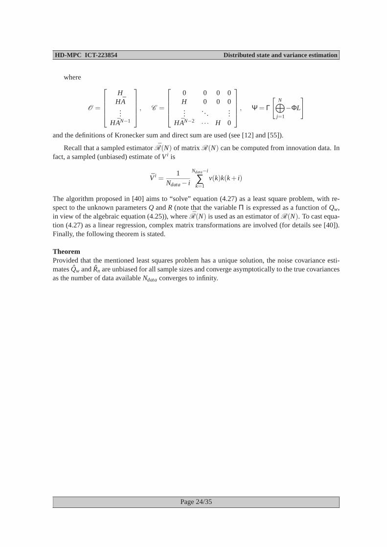
where

O =

HHA

...HAN−1

, C =

0 0 0 0H 0 0 0...

......

HAN−2 · · · H 0

, Ψ = Γ

[N⊕

j=1

−ΦL

]

and the definitions of Kronecker sum and direct sum are used (see [12] and [55]).

Recall that a sampled estimatorR(N) of matrixR(N) can be computed from innovation data. Infact, a sampled (unbiased) estimate ofV i is

V i =1

Ndata− i

Ndata−i

∑k=1

v(k)k(k+ i)

The algorithm proposed in [40] aims to “solve” equation (4.27) as a least square problem, with re-spect to the unknown parametersQ andR (note that the variableΠ is expressed as a function ofQw,in view of the algebraic equation (4.25)), whereR(N) is used as an estimator ofR(N). To cast equa-tion (4.27) as a linear regression, complex matrix transformations are involved (for details see [40]).Finally, the following theorem is stated.

TheoremProvided that the mentioned least squares problem has a unique solution, the noise covariance esti-matesQw andRn are unbiased for all sample sizes and converge asymptotically to the true covariancesas the number of data availableNdata converges to infinity.

/35


Chapter 5

Preliminary results on disturbancemodeling for distributed systems

In this Chapter, the use of disturbance models in MPC is briefly reviewed andsome introductoryconsiderations on the problem of disturbance modeling in distributed controlsystems are reported.In the MPC literature, disturbances have been considered mainly from the following two differentpoints of view:

1. disturbances modeled as (piecewise) constant signals have been included in the problem formu-lations to compute feedback control laws guaranteeing some specific properties, such as asymp-totic zero error regulation for constant reference signals, see e.g. [36], [46] and the referencesquoted there;

2. disturbances have been modeled as unknown, but bounded, signalsacting on the system stateand to be rejected by the MPC control law to guarantee some fundamental properties, such asInput-to-State Stability (ISS) or Practical ISS (p-ISS). In this case, this problem has lead to thedevelopment of robust MPC algorithms both in closed-loop and in open-loopform, see e.g.[32], [50].

These two streams of research will be very concisely summarized in the following and will berelated to the problem of designing distributed MPC laws with stability and trackingproperties.

5.1 Disturbance modeling in Model Predictive Control for offset-freetracking

In MPC, many approaches have been proposed to guarantee an offset free response for constant refer-ence signals. The most polite and effective solution is to resort to the classical approach based on theso-called Internal Model Principle (IMC), see [20], which consists ofaugmenting the process modelwith a set of integrators fed by the tracking errors. A stabilizing regulator isthen synthesized for theaugmented system. Finally, the overall regulator is composed by the ensemble of the stabilizing oneand of the integrators, i.e. of the internal model of the reference signal. The solution based on theIMC is very effective also to guarantee asymptotic zero error regulation for references generated byunstable exosystems and can be used for MPC of nonlinear process models ([30]).A criticism to IMC-based solutions applied to MPC, [36], lies in the need to enlarge the dimension ofthe system state with the internal model of the exosystem. In the case of large scale systems, this can

/35


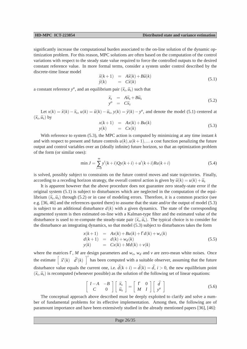
significantly increase the computational burden associated to the on-line solution of the dynamic op-timization problem. For this reason, MPC solutions are often based on the computation of the controlvariations with respect to the steady state value required to force the controlled outputs to the desiredconstant reference value. In more formal terms, consider a system under control described by thediscrete-time linear model

x(k+1) = Ax(k)+Bu(k)y(k) = Cx(k)

(5.1)

a constant referenceyo, and an equilibrium pair(xs, us) such that

xs = Axs+Bus

yo = Cxs(5.2)

Let x(k) = x(k)− xs, u(k) = u(k)− us, y(k) = y(k)− yo, and denote the model (5.1) centered at(xs, us) by

x(k+1) = Ax(k)+Bu(k)y(k) = Cx(k)

(5.3)

With reference to system (5.3), the MPC action is computed by minimizing at any time instantkand with respect to present and future controlsu(k),u(k+1), ... a cost function penalizing the futureoutput and control variables over an (ideally infinite) future horizon, sothat an optimization problemof the form (or similar ones):

min J =∞

∑i=0

y′(k+ i)Qy(k+ i)+u′(k+ i)Ru(k+ i) (5.4)

is solved, possibly subject to constraints on the future control moves and state trajectories. Finally,according to a receding horizon strategy, the overall control action is given byu(k) = u(k)+ us

It is apparent however that the above procedure does not guarantee zero steady-state error if theoriginal system (5.1) is subject to disturbances which are neglected in the computation of the equi-librium (xs, us) through (5.2) or in case of modeling errors. Therefore, it is a common practice (seee.g. [36, 46] and the references quoted there) to assume that the state and/or the output of model (5.3)is subject to an additional disturbanced(k) with a given dynamics. The state of the correspondingaugmented system is then estimated on-line with a Kalman-type filter and the estimated value of thedisturbance is used to re-compute the steady-state pair(xs, us). The typical choice is to consider forthe disturbance an integrating dynamics, so that model (5.3) subject to disturbances takes the form

x(k+1) = Ax(k)+Bu(k)+Γd(k)+wx(k)d(k+1) = d(k)+wd(k)y(k) = Cx(k)+Md(k)+v(k)

(5.5)

where the matricesΓ, M are design parameters andwx, wd andv are zero-mean white noises. Once

the estimate[

x′(k) d′(k)]′

has been computed with a suitable observer, assuming that the future

disturbance value equals the current one, i.e.d(k+ i) = d(k) = d, i > 0, the new equilibrium point(xs, us) is recomputed (whenever possible) as the solution of the following set of linear equations:

[I −A −B

C 0

][xs

us

]=

[Γ 0M I

][dyo

](5.6)

The conceptual approach above described must be deeply exploited to clarify and solve a num-ber of fundamental problems for its effective implementation. Among then, the following are ofparamount importance and have been extensively studied in the already mentioned papers [36], [46]:

/35


• the augmented system (5.5) must be observable, or detectable, to allow for the estimation of theenlarged state;

• the set of linear equations (5.6) must be solvable. This is equivalent to askfor conditions on thenumber of controlled and manipulated outputs and/or on the absence of plantinvariant zeros inz= 1;

• the steady-state pair(xs, us) must satisfy the control and state constraints of the problem. If thisdoes not hold, feasible solutions must be computed by solving suitable least-squares problems.

A critical analysis of these points is beyond the scopes of this report, and the interested readeris referred to [36], [46], [45]. However, a couple of remarks are worth recalling. First, additionaldynamics can be assumed to generate the disturbance, which turns out to begiven by the output of astable system fed by the integrators, see again [46] or [29]. This can beuseful to center the estimationand the control design in a prescribed frequency band specified by theadditional dynamics. Second,as suggested by [48], system (5.5) (with null disturbanceswx, wd, v), can be given the velocity form

∆x(k+1) = A∆x(k)+B∆u(k)z(k+1) = z(k)+CA∆x(k)+CB∆u(k)y(k) = z(k)+v(k)

(5.7)

where∆x(k) = x(k)− x(k− 1) and∆u(k) = u(k)− u(k− 1). An MPC algorithm can then be usedfor system (5.7) to compute the future control increments∆u. This implicitly corresponds to plug anintegral action on the input variables, so that an IMC-type solution is obtained. This approach tracesback to early predictive control algorithms, such as Generalized Minimum Variance (GMV), see [16],or Generalized Predictive Control (GPC), see [17], where CARIMA (Controlled AutoRegressive In-tegrating Moving Average models) were used.

In the design of MPC algorithms for distributed systems, the disturbance modeling approach de-scribed in this section can be easily extended to cope with the same objectives,such as the trackingof constant references. Specifically, given a large scale system madeby a number of interacting sub-systems, according to the previously described guidelines it is possible to design for any subsystem alocal MPC regulator guaranteeing tracking properties provided that the overall stability is achieved.In this sense, the described methodologies for disturbance modeling do notappear to be crucial tosolve the fundamental questions related to the design of distributed control laws, such as the amountof information transmitted among the subsystems and its use in the design of the control laws, therequired strength of the interconnections, the achievable stability properties.

5.2 Disturbance rejection and ISS stability in distributed control withMPC

In recent years, research in MPC has been focused in the development of algorithms guaranteeingsome fundamental stability properties also in presence of model uncertainties, parameter variations,external disturbances, see e.g. [28, 31, 51, 32, 33]. In this framework, the system under control isusually assumed to be described by

x(k+1) = f (x(k),u(k),w(k)), k≥ t, x(t) = x (5.8)

/35


where the disturbancew∈ Rq can model a wide number of the uncertainties above described; as suchit can be assumed to be either a state and control dependent term, i.e.

w(k) = fw(x(k),u(k)) (5.9)

where fw(·, ·) is a suitable function, or an external bounded signal, i.e.

w∈W (5.10)

whereW ⊆ Rq is a known compact set containing the origin.The presence of the disturbancew strongly impacts on feasibility. In fact, even though at a generic

time instantk the optimization problem is feasible, the effect of the disturbance could bringthe stateoutside the feasibility region in the next time instants. To deal with this problem, in thedesign of robustNonlinear Model Predictive Control (NMPC) algorithms a common approachconsists of consideringthe a-priori worst possible effect of the future disturbances and guaranteeing that, event in this case,feasibility is not lost. In so doing, amin-maxoptimization problem must be stated and solved, wherethe maximization is associated to the effect of the disturbance over the considered prediction horizon,while the minimization of the selected cost function must be performed with respect to the futurecontrol actions given by the control law

u(k+ i) = uop(k+ i)+κi(x(k+ i)), i = 0, ...,N−1 (5.11)

whereuop(k+ i), i = 1, ...,N are open-loop terms to be computed through the optimization problem,while the functionsκi(x) are closed-loop terms which can be either time-invariant and selected a-priorior whose parameters can be optimized on-line. The algorithms proposed in theliterature for linearand nonlinear systems can be roughly classified as follows.

• Methods where the maximization problem is solved off-line and the design parameters aresuitably modified to guarantee feasibility. In these approaches, the basic idea is to include inthe problem formulation some additional constraints on the statesx(k+ i), i = 1, ...,N predictedover the considered horizon. Specifically, the predicted statex(k+ i) is forced to belong to asetX(k+ i)⊂ X chosen so that, for any feasible disturbance sequencew(k+ j), j = 0, ..., i −1,the real state still belongs toX. The sequence of setsX(k+ i), i = 1, ...,N forms a “tube” wherethe predicted state is forced to remain. In addition, the auxiliary control law is usually chosenso that the terminal setXf is a robustly positive invariant set for the corresponding closed-loopsystem. Once the “tube” has been computed and the additional constraints onthe future stateshave been included into the problem formulation, minimization of the selected costfunction canbe performed on-line by resorting to the Receding Horizon principle. In thecontext of MPCfor nonlinear systems, [28] describes an algorithm where only the open-loop termsuop(k+ i)(5.11) are considered, while fixed closed-loop functionsκi(x(k+ i)) are used in [51].

• Methods where the whole min-max problem is solved on-line. In this case, the control law(5.11) is usually made only by the parameterized state-feedback control laws κi(x). The com-putational burden turns out to be high, but less restrictive constraints must be a-priori imposedon the state evolution over the prediction horizon. An example of application ofthis approachis described in [31].

Once the feasibility problem has been solved, the stability issue must be considered. In case ofpersistent disturbances, it is not possible to require the asymptotic stability ofthe origin, but only

/35


“practical stability”, i.e. convergence of the state trajectory to a robust positively invariant set contain-ing the origin. The size of this set obviously depends on the worst feasibledisturbance. Asymptoticstability of the origin can however be obtained for state dependent disturbances, provided that a suit-ableH∞-type cost function is used in the optimization problem, see e.g. [31]. Concerning stability, inrecent years it has been shown that the concept of Input to State Stability(ISS), see e.g. [59, 24], isthe most appropriate tool for the analysis and synthesis of robust NMPC algorithms, see [32], [50].

The robust MPC methods now described can be applied quite easily to the problem of design-ing stabilizing regulators for distributed control structures. In fact, assuming that the overall systemis made by a number of interconnected local subsystems, it is possible to see the mutual influencesamong subsystems as perturbation (disturbance) terms. In this perspective, it is advisable to designa local robust MPC law for any subsystem with robustness properties withrespect to the perturbingactions performed by the other subsystems. This approach has been already followed in [49] wherea completely decentralized and stabilizing MPC law has been designed under the main assumptionthat the interconnections are sufficiently weak. The proposed method heavily relies on the seminalresults reported in [18], which provide well sounded theoretical foundations for the analysis of inter-connected systems.Also the distributed MPC methods relying on the exchange of information among the local subsystemsregarding the future expected input or state trajectories (see the review paper [54] and the referencestherein), can be analyzed in the framework of robust MPC. In fact, it is possible to interpret the dif-ference between the predicted and the real trajectories as disturbance terms to be suitably rejected.In order to apply the results of robust MPC in this perspective, it is mandatory to impose that anylocal subsystem’s state and control trajectory does not differ too much withrespect to the predictedone transmitted to the neighborhoods, so that the “equivalent disturbanceterm” is guaranteed to bebounded. This simple consideration motivates the introduction in some algorithms of additional con-straints on the future input moves and state evolution, see for example [19] where however the MPCproblem is not explicitly based on the robustness approach.

/35


Chapter 6

Conclusions

The review of the literature on distributed state estimation reported in this deliverable has shown thatnew and efficient algorithms are required both for thedistributed estimationand for thepartition-based estimationproblems, as they have been defined in the Introduction. In fact, distributed algo-rithms with guaranteed stability and convergence properties for linear and nonlinear systems are stilllargely missing. Moreover, most of the available results rely on the Kalman filtering approach, whichcannot handle state and disturbance constraints, which are often to be considered in real problems.These considerations motivate the development of new Moving Horizon Estimation (MHE) schemes,which allow one to satisfy the two main requirements above mentioned, i.e. convergence of the es-timates and disturbance estimation. These MHE algorithms have been already partially developedfor linear systems within the project and will be extensively described in report D5.2. Further exten-sions will concern their extension to nonlinear systems as well as their applications to one or morebenchmarks, such as the hydro power valley, object of Work Package7.

As for distributed variance estimation, this is another topic of great interest. In fact, it is wellknown that the optimality properties of Kalman filters are based on the covariances of the noisesaffecting the state and measured variables. In MHE, these covariances are used to weight the termsto be minimized over a prescribed prediction horizon, namely the state disturbance and the estimationerror over the considered time window. Many case studies have shown that a poor tuning of theseweighting parameters lead to unsatisfactory results. Future research will concern the detailed analysisof the available algorithms in a number of significant cases as well as their extensions to the case ofdistributed estimation.

Finally, the wide theme of disturbance modeling can be conjugated in differentways. First, it ap-pears to be quite straightforward to extend the centralized approach for MPC with tracking propertiesby means of proper estimation of the disturbances also to distributed control structures. On the otherhand, disturbance attenuation in robust centralized model predictive control has produced a number ofmethods and results which can be exploited to design new and efficient distributed schemes where themutual interactions among locally controlled subsystems can be viewed as disturbances to be properlyrejected.

/35


Bibliography

[1] N. Abdel-Jabbar, C. Kravaris, and B. Carnaham. A partially decentralized state observer and itsparallel computer implementation.Industrial & Engineering Chemistry Research, 37(7):2741–2769, 1998.

[2] B.M. Akesson, J.B. Jørgensen, and S.B. Jørgensen. A generalized autocovariance least-squaresmethod for covariance estimation.Proc. of the American Control Conference, New York City,USA, 2007, pages 3713 – 3714, 2007.

[3] B.M. Akesson, J.B. Jørgensen, N.K. Poulsen, and S.B. Jø rgensen. A generalized autocovarianceleast-squares method for Kalman filter tuning.Journal of Process Control, 18:769–779, 2008.

[4] P. Alriksson and A. Rantzer. Distributed Kalman filtering using weighted averaging. InProc.of the 17th International Symposium on Mathematical Theory of Networksand Systems, Kyoto,Japan, 2006.

[5] P. Alriksson and A. Rantzer. Experimental evaluation of a distributed Kalman filter algorithm.In In Proc. 46th IEEE Conference on Decision and Control, pages 5499 – 5504, 2007.

[6] P. Alriksson and A. Rantzer. Model based information fusion in sensor networks. InIn Proc.17th IFAC World Congress, pages 4150–4155, Seoul, Korea, 2008.

[7] D.L. Alspach. A parallel filtering algorithm for linear systems with unknown time varying noisestatistics.IEEE Trans. on Automatic Control, 19(5):552–556, 1974.

[8] A. Averbuch, S. Itzikovitz, and T. Kapon. Radar target tracking -Viterbi versus IMM. IEEETrans. on Aerospace and Electronic Systems, 27(3):550–563, 1991.

[9] P.R. Belanger. Estimation of noise covariance matrices for a linear time-varying stochastic pro-cess.Automatica, 10:267–275, 1974.

[10] T.M. Berg and H.F. Durrant-Whyte. Model distribution in decentralized multi-sensor data fusion.In Proc. of the 10th American Control Conference, pages 2292 – 2293, 1991.

[11] T. Bohlin. Four cases of identification of changing systems.In R.K. Mehra & D.G. Lainiotis(Eds.), System Identification: Advances and case studies (1st ed.). New York: Academic Press.,1976.

[12] J. Brewer. Kronecker products and matrix calculus in systems theory. IEEE Trans. in Circuitsand Systems, 25(9):772–781, 1978.

[13] G.C. Calafiore and F. Abrate. Distributed linear estimation over sensornetworks.InternationalJournal of Control, 82(5):868 – 882, 2009.

/35


[14] B. Carew and P.R. Belanger. Identification of optimum filter steady-state gain for systems withunknown noise covariances.IEEE Trans. on Automatic Control, 18(6):582–587, 1973.

[15] R. Carli, A. Chiuso, L. Schenato, and S. Zampieri. Distributed Kalman filtering based on con-sensus strategies.IEEE Journal on Selected Areas in Communications, 4:622 – 633, 2008.

[16] D.W. Clarke and P. Gawthrop. Self-tuning control.Proc. IEE, 126:633 – 640, 1979.

[17] D.W. Clarke, C. Mohtadi, and S. Tuffs. Generalized predictive control - part I. The basic algo-rithm. Automatica, 23:137 – 148, 1987.

[18] S. Dashkovskiy, B.S. Rffer, and F.R. Wirth. An ISS theorem for general networks.Mathematicsof Control, Signals, and Systems, 19:93–122, 2007.

[19] W.B. Dunbar. Distributed receding horizon control of dynamically coupled nonlinear systems.IEEE Trans. on Automatic Control, 52:1249–1263, 2007.

[20] B.A. Francis and W. M. Wonham. The internal model principle of control theory. Automatica,12:457 – 465, 1976.

[21] H.R. Hashemipour, S. Roy, and A.J. Laub. Decentralized structures for parallel Kalman filtering.IEEE Trans. on Automatic Control, 33(1):88 – 94, January 1988.

[22] M.F. Hassan, G. Salut, M.G. Singh, and A. Titli. A decentralized computational algorithm forthe global Kalman filter.IEEE Trans. on Automatic Control, 23(2):262 – 268, 1978.

[23] C.G. Hilborn and D.G. Lainiotis. Optimal estimation in the presence of unknown parameters.IEEE Trans. on System Science and Cybernetics, 5(1):38–43, 1969.

[24] Z.-P. Jiang and Y. Wang. Input-to-state stability for discrete-time nonlinear systems.Automatica,37:857–869, 2001.

[25] M. Kamgarpour and C. Tomlin. Convergence properties of a decentralized Kalman filter.Proc.47th IEEE Conference on Decision and Control, pages 3205 – 3210, 2008.

[26] R.L. Kashyap. Maximum likelihood identification of stochastic linear systems. IEEE Trans. onAutomatic Control, 15(1):25–34, 1970.

[27] U.A. Khan and J.M.F. Moura. Distributing the Kalman filter for large-scale systems. IEEETrans. on Signal Processing, 56(10):4919 – 4935, October 2008.

[28] D. Limon, T. Alamo, and E. F. Camacho. Input-to-state stable MPC for constrained discrete-timenonlinear systems with bounded additive uncertainties. InProc. of the 41st IEEE Conference onDecision and Control, pages 4619–4624, Las Vegas, NV, USA, 2002.

[29] J. Maciejowski.Predictive Control with Constraints. Prentice Hall, 2002.

[30] L. Magni, G. De Nicolao, and R. Scattolini. Output feedback and tracking of nonlinear systemswith model predictive control.Automatica, 37:1601 – 1607, 2001.

[31] L. Magni, G. De Nicolao, R. Scattolini, and F. Allgower. Robust model predictive control ofnonlinear discrete-time systems.International Journal of Robust and Nonlinear control, 13(3-4):229–246, 2003.

/35


[32] L. Magni, D.M. Raimondo, and R. Scattolini. Regional input-to-state stability for nonlinearmodel predictive control.IEEE Trans. on Automatic Control, 51:1548–1553, 2006.

[33] L. Magni and R. Scattolini. Robustness and robust design of MPC for nonlinear systems. InR. Findeisen, L.T. Biegler, and F. Allgower, editors,Nonlinear Predictive Control, Progress inSystems Theory Series, volume 358, pages 239–254. Lecture Notes in Control and InformationSciences, Springer, 2007.

[34] R.K. Mehra. On the identification of variances and adaptive Kalman filtering. IEEE Trans. onAutomatic Control, 15(2):175–184, 1970.

[35] R.K. Mehra. Approaches to adaptive filtering.IEEE Trans. on Automatic Control, 17:903–908,1972.

[36] K.R. Muske and T.A. Badgwell. Disturbance modeling of offset-freelinear model predictivecontrol. Journal of Process Control, 12:617 – 632, 2002.

[37] A.G.O. Mutambara.Decentralized estimation and control for multisensor systems. CRC Press,1998.

[38] A.G.O. Mutambara and H.F. Durrant-Whyte. Estimation and control for amodular wheeledmobile robot.IEEE Trans. on Control Systems Technology, 8(1):35 – 46, 2000.

[39] K.A. Myers and B.D. Tapley. Adaptive sequencial estimation with unknown noise statistics.IEEE Trans. on Automatic Control, 19(5):623–625, 1976.

[40] B.J. Odelson, M.R. Rajamani, and J.B. Rawlings. A new autocovariance least-squares methodfor estimating noise covariances.Automatica, 42(2):303–308, February 2006.

[41] R. Olfati-Saber. Distributed Kalman filter with embedded consensus filters. Proc. 44th IEEEConference on Decision and Control - European Control Conference, pages 8179 – 8184, 2005.

[42] R. Olfati-Saber. Distributed Kalman filtering for sensor networks.Proc.46th IEEE Conferenceon Decision and Control, pages 5492 – 5498, 2007.

[43] R. Olfati-Saber. Kalman-consensus filter: Optimality, stability and performance. Proc. 48th

IEEE Conference on Decision and Control, pages 7036 – 7042, 2009.

[44] R. Olfati-Saber and J. Shamma. Consensus filters for sensor networks and distributed sensorfusion. Proc. 44th IEEE Conference on Decision and Control - European Control Conference,pages 6698 – 6703, 2005.

[45] G. Pannocchia and A. Bemporad. Combined design of disturbance model and observer foroffset-free model predictive control.IEEE Trans. on Automatic Control, 52:1048–1053, 2007.

[46] G. Pannocchia and J. B. Rawlings. Disturbance models for offset-free model-predictive control.AIChE Journal, 49:426 – 437, 2003.

[47] M. Perillo and W. Heinzelman.Wireless Sensor Network Protocols, Fundamental Algorithmsand Protocol for Wireless and Mobile Networks. CRC Hall, 2005.

[48] D.M. Prett and C.E. Garcia.Fundamental Process Control. Butterworths, 1988.

/35


[49] D. Raimondo, L. Magni, and R. Scattolini. Decentralized mpc of nonlinear systems: an input-to-state stability approach.Int. Journal of Robust and Nonlinear Control, 17:1651–1667, 2007.

[50] D.M. Raimondo, D. Limon, M. Lazar, L. Magni, and E.F. Camacho. Min-max model predictivecontrol of nonlinear systems: a unifying overview on stability.European Journal of Control,15:5–21, 2009.

[51] S.V. Rakovic, A.R. Teel, D.Q. Mayne, and A. Astolfi. Simple robust control invariant tubes forsome classes of nonlinear discrete time systems. InProc. of the 45th IEEE Conf. on Decisionand Control, pages 6397–6402, 2006.

[52] B.S. Rao and H.F. Durrant-Whyte. Fully decentralised algorithm for multisensor Kalman filter-ing. IEE Proc. on Control Theory and Applications, D, 138(5):413 – 420, September 1991.

[53] N. Sandell Jr, P. Varaiya, M. Athans, and M. Safonov. Surveyof decentralized control methodsfor large scale systems.IEEE Trans. on Automatic Control, 23(2):108 – 128, April 1978.

[54] R. Scattolini. Architectures for distributed and hierarchical model predictive control.Journal ofProcess Control, 19:723–731, 2009.

[55] S.R. Searle.Matrix algebra useful for statistics. New York: Wiley, 1982.

[56] J. Sijs, M. Lazar, P.P.J. Van Den Bosch, and Z. Papp. An overview of non-centralized Kalmanfilters. Proc. 17th IEEE Conference on decision and Control, pages 739–744, 2008.

[57] D.D. Siljac. Large-scale dynamic systems. Stability and structure. North Holland, 1978.

[58] D.D. Siljac and M.B. Vukcevic. On decentralized estimation.International Journal of Control,27(1):113–131, 1978.

[59] E.D. Sontag. Smooth stabilization implies coprime factorization.IEEE Trans. on AutomaticControl, 34:435–443, 1989.

[60] D.P. Spanos, R. Olfati-Saber, and R.M. Murray. Approximate distributed Kalman filtering insensor networks with quantifiable performance.Fourth International Symposium on InformationProcessing in Sensor Networks, pages 133 – 139, 2005.

[61] A. Speranzon, C. Fischione, K.H. Johansson, and Sangiovanni-Vincentelli A.L. A distributedminimum variance estimator for sensor networks.IEEE Journal on Selected Areas in Commu-nications, 26(4):609–621, 2008.

[62] S.S. Stankovic, M.S. Stankovic, and D.M. Stipanovic. Consensus based overlapping decentral-ized estimation with missing observations and communication faults.Automatica, 45:1397 –1406, 2009.

[63] S.S. Stankovic, M.S. Stankovic, and D.M. Stipanovic. Consensus based overlapping decentral-ized estimator.IEEE Trans. on Automatic Control, 54(2):410 – 415, February 2009.

[64] J. Stoustrup. Plug & play control: Control technology towards new challenges. EuropeanJournal of Control, 15(3-4):311–330, 2009.

[65] S. Tilak, N.B. Abu-Ghazaleh, and W. Heinzelman. A taxonomy of wireless micro-sensor net-work models.Mobile Computing and Communications Review, 6:28 – 32, 2002.

/35


[66] R. Vadigepalli and F.J. Doyle III. A distributed state estimation and control algorithm forplantwide processes.IEEE Trans. on Control Systems Technology, 11(1):119 – 127, January2003.

[67] R. Vadigepalli and F.J. Doyle III. structural analysis of large-scale systems for distributed stateestimation and control applications.Control Engineering Practice, 11:895 – 905, 2003.

[68] B. Warneke, M. Last, B. Liebowitz, and K.S.J. Pister. Smart dust: communicating with a cubic-millimeter computer.Computer, 34:44 – 51, 2001.

/35

SEVENTH FRAMEWORK PROGRAMME THEME – ICT [Information and … · 2010-08-26 · sults available in...

Documents

Transcript of SEVENTH FRAMEWORK PROGRAMME THEME – ICT [Information and … · 2010-08-26 · sults available in...