Chapter 9

Coping with NP-completeness

You are the junior member of a seasoned project team. Your current task is to write code forsolving a simple-looking problem involving graphs and numbers. What are you supposed todo?

If you are very lucky, your problem will be among the half-dozen problems concerninggraphs with weights (shortest path, minimum spanning tree, maximum flow, etc.), that wehave solved in this book. Even if this is the case, recognizing such a problem in its naturalhabitat—grungy and obscured by reality and context—requires practice and skill. It is morelikely that you will need to reduce your problem to one of these lucky ones—or to solve it usingdynamic programming or linear programming.

But chances are that nothing like this will happen. The world of search problems is a bleaklandscape. There are a few spots of light—brilliant algorithmic ideas—each illuminating asmall area around it (the problems that reduce to it; two of these areas, linear and dynamicprogramming, are in fact decently large). But the remaining vast expanse is pitch dark: NP-complete. What are you to do?

You can start by proving that your problem is actually NP-complete. Often a proof bygeneralization (recall the discussion on page 270 and Exercise 8.10) is all that you need; andsometimes a simple reduction from 3SAT or ZOE is not too difficult to find. This sounds like atheoretical exercise, but, if carried out successfully, it does bring some tangible rewards: nowyour status in the team has been elevated, you are no longer the kid who can’t do, and youhave become the noble knight with the impossible quest.

But, unfortunately, a problem does not go away when proved NP-complete. The real ques-tion is, What do you do next?

This is the subject of the present chapter and also the inspiration for some of the mostimportant modern research on algorithms and complexity. NP-completeness is not a deathcertificate—it is only the beginning of a fascinating adventure.

Your problem’s NP-completeness proof probably constructs graphs that are complicatedand weird, very much unlike those that come up in your application. For example, eventhough SAT is NP-complete, satisfying assignments for HORN SAT (the instances of SAT thatcome up in logic programming) can be found efficiently (recall Section 5.3). Or, suppose thegraphs that arise in your application are trees. In this case, many NP-complete problems,

283

284 Algorithms

such as INDEPENDENT SET, can be solved in linear time by dynamic programming (recallSection 6.7).

Unfortunately, this approach does not always work. For example, we know that 3SATis NP-complete. And the INDEPENDENT SET problem, along with many other NP-completeproblems, remains so even for planar graphs (graphs that can be drawn in the plane withoutcrossing edges). Moreover, often you cannot neatly characterize the instances that come upin your application. Instead, you will have to rely on some form of intelligent exponentialsearch—procedures such as backtracking and branch and bound which are exponential timein the worst-case, but, with the right design, could be very efficient on typical instances thatcome up in your application. We discuss these methods in Section 9.1.

Or you can develop an algorithm for your NP-complete optimization problem that fallsshort of the optimum but never by too much. For example, in Section 5.4 we saw that thegreedy algorithm always produces a set cover that is no more than log n times the optimalset cover. An algorithm that achieves such a guarantee is called an approximation algorithm.As we will see in Section 9.2, such algorithms are known for many NP-complete optimizationproblems, and they are some of the most clever and sophisticated algorithms around. And thetheory of NP-completeness can again be used as a guide in this endeavor, by showing that, forsome problems, there are even severe limits to how well they can be approximated—unless ofcourse P = NP.

Finally, there are heuristics, algorithms with no guarantees on either the running time orthe degree of approximation. Heuristics rely on ingenuity, intuition, a good understandingof the application, meticulous experimentation, and often insights from physics or biology, toattack a problem. We see some common kinds in Section 9.3.

9.1 Intelligent exhaustive search

9.1.1 Backtracking

Backtracking is based on the observation that it is often possible to reject a solution by lookingat just a small portion of it. For example, if an instance of SAT contains the clause (x1 ∨ x2),then all assignments with x1 = x2 = 0 (i.e., false) can be instantly eliminated. To putit differently, by quickly checking and discrediting this partial assignment, we are able toprune a quarter of the entire search space. A promising direction, but can it be systematicallyexploited?

Here’s how it is done. Consider the Boolean formula φ(w, x, y, z) specified by the set ofclauses

(w ∨ x ∨ y ∨ z), (w ∨ x), (x ∨ y), (y ∨ z), (z ∨ w), (w ∨ z).

We will incrementally grow a tree of partial solutions. We start by branching on any onevariable, say w:

S. Dasgupta, C.H. Papadimitriou, and U.V. Vazirani 285

Initial formula φ

w = 1w = 0

Plugging w = 0 and w = 1 into φ, we find that no clause is immediately violated andthus neither of these two partial assignments can be eliminated outright. So we need to keepbranching. We can expand either of the two available nodes, and on any variable of our choice.Let’s try this one:

Initial formula φ

w = 1w = 0

x = 0 x = 1

This time, we are in luck. The partial assignment w = 0, x = 1 violates the clause (w ∨ x)and can be terminated, thereby pruning a good chunk of the search space. We backtrack outof this cul-de-sac and continue our explorations at one of the two remaining active nodes.

In this manner, backtracking explores the space of assignments, growing the tree only atnodes where there is uncertainty about the outcome, and stopping if at any stage a satisfyingassignment is encountered.

In the case of Boolean satisfiability, each node of the search tree can be described eitherby a partial assignment or by the clauses that remain when those values are plugged into theoriginal formula. For instance, if w = 0 and x = 0 then any clause with w or x is instantlysatisfied and any literal w or x is not satisfied and can be removed. What’s left is

(y ∨ z), (y), (y ∨ z).

Likewise, w = 0 and x = 1 leaves(), (y ∨ z),

with the “empty clause” ( ) ruling out satisfiability. Thus the nodes of the search tree, repre-senting partial assignments, are themselves SAT subproblems.

This alternative representation is helpful for making the two decisions that repeatedlyarise: which subproblem to expand next, and which branching variable to use. Since the ben-efit of backtracking lies in its ability to eliminate portions of the search space, and since thishappens only when an empty clause is encountered, it makes sense to choose the subproblemthat contains the smallest clause and to then branch on a variable in that clause. If this clause

286 Algorithms

Figure 9.1 Backtracking reveals that φ is not satisfiable.

(), (y ∨ z)(y ∨ z), (y), (y ∨ z)

(z), (z)

(x ∨ y), (y ∨ z), (z), (z)

(x ∨ y), (y), ()(x ∨ y), ()

(w ∨ x ∨ y ∨ z), (w ∨ x), (x ∨ y), (y ∨ z), (z ∨ w), (w ∨ z)

(x ∨ y ∨ z), (x), (x ∨ y), (y ∨ z)

x = 1

()

z = 0 z = 1

()

()

y = 1

z = 1z = 0

y = 0

w = 1w = 0

x = 0

happens to be a singleton, then at least one of the resulting branches will be terminated. (Ifthere is a tie in choosing subproblems, one reasonable policy is to pick the one lowest in thetree, in the hope that it is close to a satisfying assignment.) See Figure 9.1 for the conclusionof our earlier example.

More abstractly, a backtracking algorithm requires a test that looks at a subproblem andquickly declares one of three outcomes:

1. Failure: the subproblem has no solution.

2. Success: a solution to the subproblem is found.

3. Uncertainty.

In the case of SAT, this test declares failure if there is an empty clause, success if there areno clauses, and uncertainty otherwise. The backtracking procedure then has the followingformat.

Start with some problem P0

Let S = {P0}, the set of active subproblemsRepeat while S is nonempty:choose a subproblem P ∈ S and remove it from Sexpand it into smaller subproblems P1, P2, . . . , Pk

For each Pi:If test(Pi) succeeds: halt and announce this solutionIf test(Pi) fails: discard Pi

S. Dasgupta, C.H. Papadimitriou, and U.V. Vazirani 287

Otherwise: add Pi to SAnnounce that there is no solution

For SAT, the choose procedure picks a clause, and expand picks a variable within that clause.We have already discussed some reasonable ways of making such choices.

With the right test, expand, and choose routines, backtracking can be remarkably effec-tive in practice. The backtracking algorithm we showed for SAT is the basis of many successfulsatisfiability programs. Another sign of quality is this: if presented with a 2SAT instance, itwill always find a satisfying assignment, if one exists, in polynomial time (Exercise 9.1)!

9.1.2 Branch-and-boundThe same principle can be generalized from search problems such as SAT to optimizationproblems. For concreteness, let’s say we have a minimization problem; maximization willfollow the same pattern.

As before, we will deal with partial solutions, each of which represents a subproblem,namely, what is the (cost of the) best way to complete this solution? And as before, we needa basis for eliminating partial solutions, since there is no other source of efficiency in ourmethod. To reject a subproblem, we must be certain that its cost exceeds that of some othersolution we have already encountered. But its exact cost is unknown to us and is generallynot efficiently computable. So instead we use a quick lower bound on this cost.

Start with some problem P0

Let S = {P0}, the set of active subproblemsbestsofar=∞Repeat while S is nonempty:choose a subproblem (partial solution) P ∈ S and remove it from Sexpand it into smaller subproblems P1, P2, . . . , Pk

For each Pi:If Pi is a complete solution: update bestsofarelse if lowerbound(Pi) < bestsofar: add Pi to S

return bestsofar

Let’s see how this works for the traveling salesman problem on a graph G = (V,E) withedge lengths de > 0. A partial solution is a simple path a b passing through some verticesS ⊆ V , where S includes the endpoints a and b. We can denote such a partial solution by thetuple [a, S, b]—in fact, awill be fixed throughout the algorithm. The corresponding subproblemis to find the best completion of the tour, that is, the cheapest complementary path b a withintermediate nodes V −S. Notice that the initial problem is of the form [a, {a}, a] for any a ∈ Vof our choosing.

At each step of the branch-and-bound algorithm, we extend a particular partial solution[a, S, b] by a single edge (b, x), where x ∈ V −S. There can be up to |V −S| ways to do this, andeach of these branches leads to a subproblem of the form [a, S ∪ {x}, x].

288 Algorithms

How can we lower-bound the cost of completing a partial tour [a, S, b]? Many sophisticatedmethods have been developed for this, but let’s look at a rather simple one. The remainder ofthe tour consists of a path through V −S, plus edges from a and b to V −S. Therefore, its costis at least the sum of the following:

1. The lightest edge from a to V − S.

2. The lightest edge from b to V − S.

3. The minimum spanning tree of V − S.

(Do you see why?) And this lower bound can be computed quickly by a minimum spanningtree algorithm. Figure 9.2 runs through an example: each node of the tree represents a partialtour (specifically, the path from the root to that node) that at some stage is considered by thebranch-and-bound procedure. Notice how just 28 partial solutions are considered, instead ofthe 7! = 5,040 that would arise in a brute-force search.

S. Dasgupta, C.H. Papadimitriou, and U.V. Vazirani 289

Figure 9.2 (a) A graph and its optimal traveling salesman tour. (b) The branch-and-boundsearch tree, explored left to right. Boxed numbers indicate lower bounds on cost.

(a)

A B

C

D

EF

G

H1

2

1

11

21

2

5

1 11

A B

C

D

EF

G

H1 1

11

1

1 11

(b)

A

E

HF

G

B

F

G

D15

14

8

B D

C

D H

G

H8

E C G

inf

8

10

13

12

8

814

8

8

8

8

10

C10

GE

F

G

H

D

11

11

11

11

inf

H

G14

1410 10

Cost: 11 Cost: 8

290 Algorithms

9.2 Approximation algorithmsIn an optimization problem we are given an instance I and are asked to find the optimumsolution—the one with the maximum gain if we have a maximization problem like INDEPEN-DENT SET, or the minimum cost if we are dealing with a minimization problem such as theTSP. For every instance I, let us denote by OPT(I) the value (benefit or cost) of the optimumsolution. It makes the math a little simpler (and is not too far from the truth) to assume thatOPT(I) is always a positive integer.

We have already seen an example of a (famous) approximation algorithm in Section 5.4:the greedy scheme for SET COVER. For any instance I of size n, we showed that this greedyalgorithm is guaranteed to quickly find a set cover of cardinality at most OPT(I) log n. Thislog n factor is known as the approximation guarantee of the algorithm.

More generally, consider any minimization problem. Suppose now that we have an algo-rithm A for our problem which, given an instance I, returns a solution with value A(I). Theapproximation ratio of algorithm A is defined to be

αA = maxI

A(I)

OPT(I).

In other words, αA measures by the factor by which the output of algorithm A exceeds theoptimal solution, on the worst-case input. The approximation ratio can also be defined formaximization problems, such as INDEPENDENT SET, in the same way—except that to get anumber larger than 1 we take the reciprocal.

So, when faced with an NP-complete optimization problem, a reasonable goal is to look foran approximation algorithm A whose αA is as small as possible. But this kind of guaranteemight seem a little puzzling: How can we come close to the optimum if we cannot determinethe optimum? Let’s look at a simple example.

9.2.1 Vertex coverWe already know the VERTEX COVER problem is NP-hard.

VERTEX COVER

Input: An undirected graph G = (V,E).Output: A subset of the vertices S ⊆ V that touches every edge.Goal: Minimize |S|.

See Figure 9.3 for an example.Since VERTEX COVER is a special case of SET COVER, we know from Chapter 5 that it can

be approximated within a factor of O(log n) by the greedy algorithm: repeatedly delete thevertex of highest degree and include it in the vertex cover. And there are graphs on which thegreedy algorithm returns a vertex cover that is indeed log n times the optimum.

A better approximation algorithm for VERTEX COVER is based on the notion of a matching,a subset of edges that have no vertices in common (Figure 9.4). A matching is maximal if no

S. Dasgupta, C.H. Papadimitriou, and U.V. Vazirani 291

Figure 9.3 A graph whose optimal vertex cover, shown shaded, is of size 8.

Figure 9.4 (a) A matching, (b) its completion to a maximal matching, and (c) the resultingvertex cover.(a) (b) (c)

more edges can be added to it. Maximal matchings will help us find good vertex covers, andmoreover, they are easy to generate: repeatedly pick edges that are disjoint from the oneschosen already, until this is no longer possible.

What is the relationship between matchings and vertex covers? Here is the crucial fact:any vertex cover of a graphGmust be at least as large as the number of edges in any matchingin G; that is, any matching provides a lower bound on OPT. This is simply because each edgeof the matching must be covered by one of its endpoints in any vertex cover! Finding such alower bound is a key step in designing an approximation algorithm, because we must comparethe quality of the solution found by our algorithm to OPT, which is NP-complete to compute.

One more observation completes the design of our approximation algorithm: let S be aset that contains both endpoints of each edge in a maximal matching M . Then S must be avertex cover—if it isn’t, that is, if it doesn’t touch some edge e ∈ E, then M could not possiblybe maximal since we could still add e to it. But our cover S has 2|M | vertices. And from theprevious paragraph we know that any vertex cover must have size at least |M |. So we’re done.

Here’s the algorithm for VERTEX COVER.

Find a maximal matching M ⊆ E

292 Algorithms

Return S = {all endpoints of edges in M}

This simple procedure always returns a vertex cover whose size is at most twice optimal!In summary, even though we have no way of finding the best vertex cover, we can easily

find another structure, a maximal matching, with two key properties:

1. Its size gives us a lower bound on the optimal vertex cover.

2. It can be used to build a vertex cover, whose size can be related to that of the optimalcover using property 1.

Thus, this simple algorithm has an approximation ratio of αA ≤ 2. In fact, it is not hard tofind examples on which it does make a 100% error; hence αA = 2.

9.2.2 ClusteringWe turn next to a clustering problem, in which we have some data (text documents, say, orimages, or speech samples) that we want to divide into groups. It is often useful to define “dis-tances” between these data points, numbers that capture how close or far they are from oneanother. Often the data are true points in some high-dimensional space and the distances arethe usual Euclidean distance; in other cases, the distances are the result of some “similaritytests” to which we have subjected the data points. Assume that we have such distances andthat they satisfy the usual metric properties:

1. d(x, y) ≥ 0 for all x, y.

2. d(x, y) = 0 if and only if x = y.

3. d(x, y) = d(y, x).

4. (Triangle inequality) d(x, y) ≤ d(x, z) + d(z, y).

We would like to partition the data points into groups that are compact in the sense of havingsmall diameter.

k-CLUSTER

Input: Points X = {x1, . . . , xn} with underlying distance metric d(·, ·); integer k.Output: A partition of the points into k clusters C1, . . . , Ck.Goal: Minimize the diameter of the clusters,

maxj

maxxa,xb∈Cj

d(xa, xb).

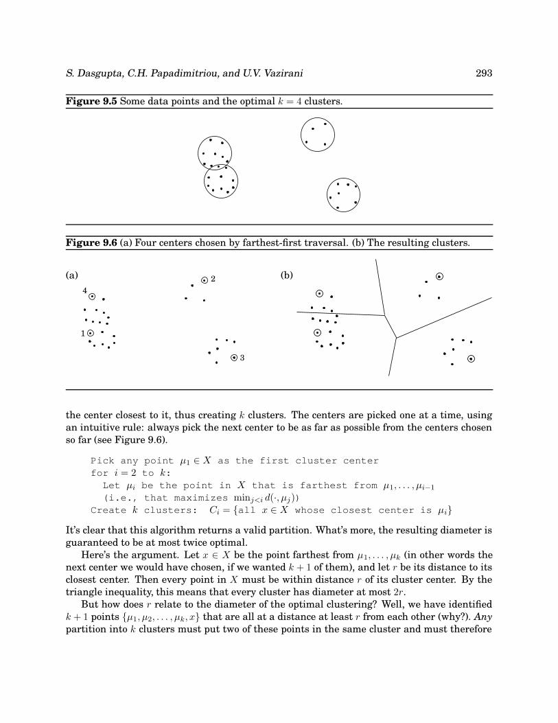
One way to visualize this task is to imagine n points in space, which are to be covered by kspheres of equal size. What is the smallest possible diameter of the spheres? Figure 9.5 showsan example.

This problem is NP-hard, but has a very simple approximation algorithm. The idea is topick k of the data points as cluster centers and to then assign each of the remaining points to

S. Dasgupta, C.H. Papadimitriou, and U.V. Vazirani 293

Figure 9.5 Some data points and the optimal k = 4 clusters.

Figure 9.6 (a) Four centers chosen by farthest-first traversal. (b) The resulting clusters.

(a) 2

1

4

3

(b)

the center closest to it, thus creating k clusters. The centers are picked one at a time, usingan intuitive rule: always pick the next center to be as far as possible from the centers chosenso far (see Figure 9.6).

Pick any point µ1 ∈ X as the first cluster centerfor i = 2 to k:Let µi be the point in X that is farthest from µ1, . . . , µi−1

(i.e., that maximizes minj<i d(·, µj))Create k clusters: Ci = {all x ∈ X whose closest center is µi}

It’s clear that this algorithm returns a valid partition. What’s more, the resulting diameter isguaranteed to be at most twice optimal.

Here’s the argument. Let x ∈ X be the point farthest from µ1, . . . , µk (in other words thenext center we would have chosen, if we wanted k + 1 of them), and let r be its distance to itsclosest center. Then every point in X must be within distance r of its cluster center. By thetriangle inequality, this means that every cluster has diameter at most 2r.

But how does r relate to the diameter of the optimal clustering? Well, we have identifiedk + 1 points {µ1, µ2, . . . , µk, x} that are all at a distance at least r from each other (why?). Anypartition into k clusters must put two of these points in the same cluster and must therefore

294 Algorithms

have diameter at least r.

This algorithm has a certain high-level similarity to our scheme for VERTEX COVER. In-stead of a maximal matching, we use a different easily computable structure—a set of k pointsthat cover all of X within some radius r, while at the same time being mutually separatedby a distance of at least r. This structure is used both to generate a clustering and to give alower bound on the optimal clustering.

We know of no better approximation algorithm for this problem.

9.2.3 TSPThe triangle inequality played a crucial role in making the k-CLUSTER problem approximable.It also helps with the TRAVELING SALESMAN PROBLEM: if the distances between cities satisfythe metric properties, then there is an algorithm that outputs a tour of length at most 1.5times optimal. We’ll now look at a slightly weaker result that achieves a factor of 2.

Continuing with the thought processes of our previous two approximation algorithms, wecan ask whether there is some structure that is easy to compute and that is plausibly relatedto the best traveling salesman tour (as well as providing a good lower bound on OPT). A littlethought and experimentation reveals the answer to be the minimum spanning tree.

Let’s understand this relation. Removing any edge from a traveling salesman tour leavesa path through all the vertices, which is a spanning tree. Therefore,

TSP cost ≥ cost of this path ≥ MST cost.

Now, we somehow need to use the MST to build a traveling salesman tour. If we can use eachedge twice, then by following the shape of the MST we end up with a tour that visits all thecities, some of them more than once. Here’s an example, with the MST on the left and theresulting tour on the right (the numbers show the order in which the edges are taken).

TulsaAlbuquerque Amarillo

Wichita

LittleRock

Dallas

Houston

San Antonio

El Paso

Tulsa

Wichita

LittleRock

Dallas

HoustonEl Paso

Amarillo

San Antonio

Albuquerque

5

2

1

109

11

8 7

12

6

4

13

14

3

1516

Therefore, this tour has a length at most twice the MST cost, which as we’ve already seen isat most twice the TSP cost.

This is the result we wanted, but we aren’t quite done because our tour visits some citiesmultiple times and is therefore not legal. To fix the problem, the tour should simply skip anycity it is about to revisit, and instead move directly to the next new city in its list:

S. Dasgupta, C.H. Papadimitriou, and U.V. Vazirani 295

Tulsa

Wichita

LittleRock

Dallas

Houston

San Antonio

El Paso

Albuquerque

Amarillo

By the triangle inequality, these bypasses can only make the overall tour shorter.

General TSP

But what if we are interested in instances of TSP that do not satisfy the triangle inequality?It turns out that this is a much harder problem to approximate.

Here is why: Recall that on page 274 we gave a polynomial-time reduction which givenany graph G and integer any C > 0 produces an instance I(G,C) of the TSP such that:

(i) If G has a Rudrata path, then OPT(I(G,C)) = n, the number of vertices in G.

(ii) If G has no Rudrata path, then OPT(I(G,C)) ≥ n+ C.

This means that even an approximate solution to TSP would enable us to solve RUDRATAPATH! Let’s work out the details.

Consider an approximation algorithmA for TSP and let αA denote its approximation ratio.From any instance G of RUDRATA PATH, we will create an instance I(G,C) of TSP using thespecific constant C = nαA. What happens when algorithm A is run on this TSP instance? Incase (i), it must output a tour of length at most αAOPT(I(G,C)) = nαA, whereas in case (ii) itmust output a tour of length at least OPT(I(G,C)) > nαA. Thus we can figure out whether Ghas a Rudrata path! Here is the resulting procedure:

Given any graph G:compute I(G,C) (with C = n · αA) and run algorithm A on itif the resulting tour has length ≤ nαA:

conclude that G has a Rudrata pathelse: conclude that G has no Rudrata path

This tells us whether or not G has a Rudrata path; by calling the procedure a polynomialnumber of times, we can find the actual path (Exercise 8.2).

We’ve shown that if TSP has a polynomial-time approximation algorithm, then there isa polynomial algorithm for the NP-complete RUDRATA PATH problem. So, unless P = NP,there cannot exist an efficient approximation algorithm for the TSP.

296 Algorithms

9.2.4 KnapsackOur last approximation algorithm is for a maximization problem and has a very impressiveguarantee: given any ε > 0, it will return a solution of value at least (1− ε) times the optimalvalue, in time that scales only polynomially in the input size and in 1/ε.

The problem is KNAPSACK, which we first encountered in Chapter 6. There are n items,with weights w1, . . . , wn and values v1, . . . , vn (all positive integers), and the goal is to pick themost valuable combination of items subject to the constraint that their total weight is at mostW .

Earlier we saw a dynamic programming solution to this problem with running timeO(nW ).Using a similar technique, a running time of O(nV ) can also be achieved, where V is the sumof the values. Neither of these running times is polynomial, because W and V can be verylarge, exponential in the size of the input.

Let’s consider the O(nV ) algorithm. In the bad case when V is large, what if we simplyscale down all the values in some way? For instance, if

v1 = 117,586,003, v2 = 738,493,291, v3 = 238,827,453,

we could simply knock off some precision and instead use 117, 738, and 238. This doesn’tchange the problem all that much and will make the algorithm much, much faster!

Now for the details. Along with the input, the user is assumed to have specified someapproximation factor ε > 0.

Discard any item with weight > WLet vmax = maxi vi

Rescale values vi = bvi · nεvmaxc

Run the dynamic programming algorithm with values {vi}Output the resulting choice of items

Let’s see why this works. First of all, since the rescaled values vi are all at most n/ε, thedynamic program is efficient, running in time O(n3/ε).

Now suppose the optimal solution to the original problem is to pick some subset of itemsS, with total value K∗. The rescaled value of this same assignment is

∑

i∈S

vi =∑

i∈S

⌊vi ·

n

εvmax

⌋≥∑

i∈S

(vi ·

n

εvmax− 1

)≥ K∗ · n

εvmax− n.

Therefore, the optimal assignment for the shrunken problem, call it S, has a rescaled value ofat least this much. In terms of the original values, assignment S has a value of at least

∑

i∈bS

vi ≥∑

i∈bS

vi ·εvmaxn

≥(K∗ · n

εvmax− n

)· εvmax

n= K∗ − εvmax ≥ K∗(1− ε).

S. Dasgupta, C.H. Papadimitriou, and U.V. Vazirani 297

9.2.5 The approximability hierarchyGiven any NP-complete optimization problem, we seek the best approximation algorithmpossible. Failing this, we try to prove lower bounds on the approximation ratios that areachievable in polynomial time (we just carried out such a proof for the general TSP). All told,NP-complete optimization problems are classified as follows:

• Those for which, like the TSP, no finite approximation ratio is possible.

• Those for which an approximation ratio is possible, but there are limits to how smallthis can be. VERTEX COVER, k-CLUSTER, and the TSP with triangle inequality belonghere. (For these problems we have not established limits to their approximability, butthese limits do exist, and their proofs constitute some of the most sophisticated resultsin this field.)

• Down below we have a more fortunate class of NP-complete problems for which ap-proximability has no limits, and polynomial approximation algorithms with error ratiosarbitrarily close to zero exist. KNAPSACK resides here.

• Finally, there is another class of problems, between the first two given here, for whichthe approximation ratio is about log n. SET COVER is an example.

(A humbling reminder: All this is contingent upon the assumption P 6= NP. Failing this,this hierarchy collapses down to P, and all NP-complete optimization problems can be solvedexactly in polynomial time.)

A final point on approximation algorithms: often these algorithms, or their variants, per-form much better on typical instances than their worst-case approximation ratio would haveyou believe.

9.3 Local search heuristicsOur next strategy for coping with NP-completeness is inspired by evolution (which is, afterall, the world’s best-tested optimization procedure)—by its incremental process of introducingsmall mutations, trying them out, and keeping them if they work well. This paradigm iscalled local search and can be applied to any optimization task. Here’s how it looks for aminimization problem.

let s be any initial solutionwhile there is some solution s′ in the neighborhood of s

for which cost(s′) < cost(s): replace s by s′

return s

On each iteration, the current solution is replaced by a better one close to it, in its neigh-borhood. This neighborhood structure is something we impose upon the problem and is thecentral design decision in local search. As an illustration, let’s revisit the traveling salesmanproblem.

298 Algorithms

9.3.1 Traveling salesman, once moreAssume we have all interpoint distances between n cities, giving a search space of (n − 1)!different tours. What is a good notion of neighborhood?

The most obvious notion is to consider two tours as being close if they differ in just a fewedges. They can’t differ in just one edge (do you see why?), so we will consider differences oftwo edges. We define the 2-change neighborhood of tour s as being the set of tours that can beobtained by removing two edges of s and then putting in two other edges. Here’s an exampleof a local move:

We now have a well-defined local search procedure. How does it measure up under our twostandard criteria for algorithms—what is its overall running time, and does it always returnthe best solution?

Embarrassingly, neither of these questions has a satisfactory answer. Each iteration iscertainly fast, because a tour has only O(n2) neighbors. However, it is not clear how manyiterations will be needed: whether for instance, there might be an exponential number ofthem. Likewise, all we can easily say about the final tour is that it is locally optimal—thatis, it is superior to the tours in its immediate neighborhood. There might be better solutionsfurther away. For instance, the following picture shows a possible final answer that is clearlysuboptimal; the range of local moves is simply too limited to improve upon it.

To overcome this, we may try a more generous neighborhood, for instance 3-change, con-sisting of tours that differ on up to three edges. And indeed, the preceding bad case getsfixed:

But there is a downside, in that the size of a neighborhood becomes O(n3), making eachiteration more expensive. Moreover, there may still be suboptimal local minima, althoughfewer than before. To avoid these, we would have to go up to 4-change, or higher. In thismanner, efficiency and quality often turn out to be competing considerations in a local search.Efficiency demands neighborhoods that can be searched quickly, but smaller neighborhoods

S. Dasgupta, C.H. Papadimitriou, and U.V. Vazirani 299

can increase the abundance of low-quality local optima. The appropriate compromise is typi-cally determined by experimentation.

300 Algorithms

Figure 9.7 (a) Nine American cities. (b) Local search, starting at a random tour, and using3-change. The traveling salesman tour is found after three moves.

(a)

TulsaAlbuquerque Amarillo

Wichita

LittleRock

Dallas

Houston

San Antonio

El Paso

(b)

(i) (ii)

(iii) (iv)

S. Dasgupta, C.H. Papadimitriou, and U.V. Vazirani 301

Figure 9.8 Local search.

Figure 9.7 shows a specific example of local search at work. Figure 9.8 is a more abstract,stylized depiction of local search. The solutions crowd the unshaded area, and cost decreaseswhen we move downward. Starting from an initial solution, the algorithm moves downhilluntil a local optimum is reached.

In general, the search space might be riddled with local optima, and some of them maybe of very poor quality. The hope is that with a judicious choice of neighborhood structure,most local optima will be reasonable. Whether this is the reality or merely misplaced faith,it is an empirical fact that local search algorithms are the top performers on a broad range ofoptimization problems. Let’s look at another such example.

9.3.2 Graph partitioningThe problem of graph partitioning arises in a diversity of applications, from circuit layoutto program analysis to image segmentation. We saw a special case of it, BALANCED CUT, inChapter 8.

GRAPH PARTITIONING

Input: An undirected graph G = (V,E) with nonnegative edge weights; a realnumber α ∈ (0, 1/2].Output: A partition of the vertices into two groups A and B, each of size at leastα|V |.Goal: Minimize the capacity of the cut (A,B).

302 Algorithms

Figure 9.9 An instance of GRAPH PARTITIONING, with the optimal partition for α = 1/2.Vertices on one side of the cut are shaded.

Figure 9.9 shows an example in which the graph has 16 nodes, all edge weights are 0or 1, and the optimal solution has cost 0. Removing the restriction on the sizes of A and Bwould give the MINIMUM CUT problem, which we know to be efficiently solvable using flowtechniques. The present variant, however, is NP-hard. In designing a local search algorithm,it will be a big convenience to focus on the special case α = 1/2, in which A and B are forced tocontain exactly half the vertices. The apparent loss of generality is purely cosmetic, as GRAPHPARTITIONING reduces to this particular case.

We need to decide upon a neighborhood structure for our problem, and there is one obviousway to do this. Let (A,B), with |A| = |B|, be a candidate solution; we will define its neighborsto be all solutions obtainable by swapping one pair of vertices across the cut, that is, allsolutions of the form (A− {a}+ {b}, B − {b}+ {a}) where a ∈ A and b ∈ B. Here’s an exampleof a local move:

We now have a reasonable local search procedure, and we could just stop here. But thereis still a lot of room for improvement in terms of the quality of the solutions produced. Thesearch space includes some local optima that are quite far from the global solution. Here’sone which has cost 2.

S. Dasgupta, C.H. Papadimitriou, and U.V. Vazirani 303

What can be done about such suboptimal solutions? We could expand the neighborhood sizeto allow two swaps at a time, but this particular bad instance would still stubbornly resist.Instead, let’s look at some other generic schemes for improving local search procedures.

9.3.3 Dealing with local optimaRandomization and restartsRandomization can be an invaluable ally in local search. It is typically used in two ways: topick a random initial solution, for instance a random graph partition; and to choose a localmove when several are available.

When there are many local optima, randomization is a way of making sure that there is atleast some probability of getting to the right one. The local search can then be repeated severaltimes, with a different random seed on each invocation, and the best solution returned. If theprobability of reaching a good local optimum on any given run is p, then within O(1/p) runssuch a solution is likely to be found (recall Exercise 1.34).

Figure 9.10 shows a small instance of graph partitioning, along with the search space ofsolutions. There are a total of

(84

)= 70 possible states, but since each of them has an identical

twin in which the left and right sides of the cut are flipped, in effect there are just 35 solutions.In the figure, these are organized into seven groups for readability. There are five local optima,of which four are bad, with cost 2, and one is good, with cost 0. If local search is started at arandom solution, and at each step a random neighbor of lower cost is selected, then the searchis at most four times as likely to wind up in a bad solution than a good one. Thus only a smallhandful of repetitions is needed.

304 Algorithms

Figure 9.10 The search space for a graph with eight nodes. The space contains 35 solutions,which have been partitioned into seven groups for clarity. An example of each is shown. Thereare five local optima.

4 states, cost 2

1 state, cost 0

8 states, cost 3

8 states, cost 4

4 states, cost 6

2 states, cost 4

8 states, cost 3

S. Dasgupta, C.H. Papadimitriou, and U.V. Vazirani 305

Simulated annealingIn the example of Figure 9.10, each run of local search has a reasonable chance of finding theglobal optimum. This isn’t always true. As the problem size grows, the ratio of bad to goodlocal optima often increases, sometimes to the point of being exponentially large. In suchcases, simply repeating the local search a few times is ineffective.

A different avenue of attack is to occasionally allow moves that actually increase the cost,in the hope that they will pull the search out of dead ends. This would be very useful at thebad local optima of Figure 9.10, for instance. The method of simulated annealing redefinesthe local search by introducing the notion of a temperature T .

let s be any starting solutionrepeat

randomly choose a solution s′ in the neighborhood of sif ∆ = cost(s′)− cost(s) is negative:

replace s by s′

else:replace s by s′ with probability e−∆/T.

If T is zero, this is identical to our previous local search. But if T is large, then moves thatincrease the cost are occasionally accepted. What value of T should be used?

The trick is to start with T large and then gradually reduce it to zero. Thus initially,the local search can wander around quite freely, with only a mild preference for low-costsolutions. As time goes on, this preference becomes stronger, and the system mostly sticks tothe lower-cost region of the search space, with occasional excursions out of it to escape localoptima. Eventually, when the temperature drops further, the system converges on a solution.Figure 9.11 shows this process schematically.

Simulated annealing is inspired by the physics of crystallization. When a substance is tobe crystallized, it starts in liquid state, with its particles in relatively unconstrained motion.Then it is slowly cooled, and as this happens, the particles gradually move into more regularconfigurations. This regularity becomes more and more pronounced until finally a crystallattice is formed.

The benefits of simulated annealing come at a significant cost: because of the changingtemperature and the initial freedom of movement, many more local moves are needed untilconvergence. Moreover, it is quite an art to choose a good timetable by which to decrease thetemperature, called an annealing schedule. But in many cases where the quality of solutionsimproves significantly, the tradeoff is worthwhile.

306 Algorithms

Figure 9.11 Simulated annealing.

Exercises9.1. In the backtracking algorithm for SAT, suppose that we always choose a subproblem (CNF

formula) that has a clause that is as small as possible; and we expand it along a variable thatappears in this small clause. Show that this is a polynomial-time algorithm in the special casein which the input formula has only clauses with two literals (that is, it is an instance of 2SAT).

9.2. Devise a backtracking algorithm for the RUDRATA PATH problem from a fixed vertex s. To fullyspecify such an algorithm you must define:

(a) What is a subproblem?(b) How to choose a subproblem.(c) How to expand a subproblem.

Argue briefly why your choices are reasonable.

9.3. Devise a branch-and-bound algorithm for the SET COVER problem. This entails deciding:

(a) What is a subproblem?(b) How do you choose a subproblem to expand?(c) How do you expand a subproblem?(d) What is an appropriate lowerbound?

Do you think that your choices above will work well on typical instances of the problem? Why?

9.4. Given an undirected graphG = (V,E) in which each node has degree≤ d, show how to efficientlyfind an independent set whose size is at least 1/(d+ 1) times that of the largest independent set.

9.5. Local search for minimum spanning trees. Consider the set of all spanning trees (not just mini-mum ones) of a weighted, connected, undirected graph G = (V,E).

S. Dasgupta, C.H. Papadimitriou, and U.V. Vazirani 307

Recall from Section 5.1 that adding an edge e to a spanning tree T creates an unique cycle, andsubsequently removing any other edge e′ 6= e from this cycle gives back a different spanning treeT ′. We will say that T and T ′ differ by a single edge swap (e, e′) and that they are neighbors.

(a) Show that it is possible to move from any spanning tree T to any other spanning tree T ′ byperforming a series of edge-swaps, that is, by moving from neighbor to neighbor. At mosthow many edge-swaps are needed?

(b) Show that if T ′ is an MST, then it is possible to choose these swaps so that the costs ofthe spanning trees encountered along the way are nonincreasing. In other words, if thesequence of spanning trees encountered is

T = T0 → T1 → T2 → · · · → Tk = T ′,

then cost(Ti+1) ≤ cost(Ti) for all i < k.(c) Consider the following local search algorithm which is given as input an undirected graph

G.Let T be any spanning tree of Gwhile there is an edge-swap (e, e′) which reduces cost(T ):

T ← T + e− e′return T

Show that this procedure always returns a minimum spanning tree. At most how manyiterations does it take?

9.6. In the MINIMUM STEINER TREE problem, the input consists of: a complete graph G = (V,E)with distances duv between all pairs of nodes; and a distinguished set of terminal nodes V ′ ⊆ V .The goal is to find a minimum-cost tree that includes the vertices V ′. This tree may or may notinclude nodes in V − V ′.

Suppose the distances in the input are a metric (recall the definition on page 292). Show thatan efficient ratio-2 approximation algorithm for MINIMUM STEINER TREE can be obtained byignoring the nonterminal nodes and simply returning the minimum spanning tree on V ′. (Hint:Recall our approximation algorithm for the TSP.)

9.7. In the MULTIWAY CUT problem, the input is an undirected graphG = (V,E) and a set of terminalnodes s1, s2, . . . , sk ∈ V . The goal is to find the minimum set of edges in E whose removal leavesall terminals in different components.

(a) Show that this problem can be solved exactly in polynomial time when k = 2.(b) Give an approximation algorithm with ratio at most 2 for the case k = 3.(c) Design a local search algorithm for multiway cut.

308 Algorithms

9.8. In the MAX SAT problem, we are given a set of clauses, and we want to find an assignment thatsatisfies as many of them as possible.

(a) Show that if this problem can be solved in polynomial time, then so can SAT.(b) Here’s a very naive algorithm.

for each variable:set its value to either 0 or 1 by flipping a coin

Suppose the input has m clauses, of which the jth has kj literals. Show that the expectednumber of clauses satisfied by this simple algorithm is

m∑

j=1

(1− 1

2kj

)≥ m

2.

In other words, this is a 2-approximation in expectation! And if the clauses all contain kliterals, then this approximation factor improves to 1 + 1/(2k − 1).

(c) Can you make this algorithm deterministic? (Hint: Instead of flipping a coin for eachvariable, select the value that satisfies the most of the as of yet unsatisfied clauses. Whatfraction of the clauses is satisfied in the end?)

9.9. In the MAXIMUM CUT problem we are given an undirected graph G = (V,E) with a weight w(e)on each edge, and we wish to separate the vertices into two sets S and V − S so that the totalweight of the edges between the two sets is as large as possible.For each S ⊆ V define w(S) to be the sum of all w(e) over all edges {u, v} such that |S∩{u, v}| = 1.Obviously, MAX CUT is about maximizing w(S) over all subsets of V .Consider the following local search algorithm for MAX CUT:

start with any S ⊆ Vwhile there is a subset S′ ⊆ V such that||S′| − |S|| = 1 and w(S′) > w(S) do:

set S = S′

(a) Show that this is an approximation algorithm for MAX CUT with ratio 2.(b) But is it a polynomial-time algorithm?

9.10. Let us call a local search algorithm exact when it always produces the optimum solution. Forexample, the local search algorithm for the minimum spanning tree problem introduced in Prob-lem 9.5 is exact. For another example, simplex can be considered an exact local search algorithmfor linear programming.

(a) Show that the 2-change local search algorithm for the TSP is not exact.(b) Repeat for the dn

2 e-change local search algorithm, where n is the number of cities.(c) Show that the (n− 1)-change local search algorithm is exact.(d) IfA is an optimization problem, defineA-IMPROVEMENT to be the following search problem:

Given an instance x of A and a solution s of A, find another solution of x with better cost (orreport that none exists, and thus s is optimum). For example, in TSP IMPROVEMENT we aregiven a distance matrix and a tour, and we are asked to find a better tour. It turns out thatTSP IMPROVEMENT is NP-complete, and so is SET COVER IMPROVEMENT. (Can you provethis?)

S. Dasgupta, C.H. Papadimitriou, and U.V. Vazirani 309

(e) We say that a local search algorithm has polynomial iteration if each execution of the looprequires polynomial time. For example, the obvious implementations of the (n − 1)-changelocal search algorithm for the TSP defined above do not have polynomial iteration. Showthat, unless P = NP, there is no exact local search algorithm with polynomial iteration forthe TSP and SET COVER problems.