SEVENTH FRAMEWORK PROGRAMME THEME – ICT … · HD-MPC ICT-223854 HD-MPC validation for the Hydro...

SEVENTH FRAMEWORK PROGRAMME THEME – ICT

[Information and Communication Technologies]

Contract Number: 223854 Project Title: Hierarchical and Distributed Model Predictive

Control of Large-Scale Systems Project Acronym: HD-MPC

Deliverable Number: D7.2.3 Part I Deliverable Type: Report Contractual Date of Delivery: November 1, 2011 Actual Date of Delivery: November 1, 2011 Title of Deliverable: Report that presents the closed-loop validation

results for the hydro-power valley, including stability and constraints issues, as well as the HD-MPC demonstration of results – Part I

Dissemination level: P Workpackage contributing to the Deliverable: WP7 WP Leader: Damien Faille Partners: EDF, SUPELEC Author(s): D. Faille, F. Davelaar, S. Murgey, D. Dumur

Copyright by the HD-MPC Consortium

HD-MPC ICT-223854 HD-MPC validation for the Hydro Power Valley – Part I

/27

Table of Content

1 SYNOPSIS....................................................................................................................................................... 4

2 HPV MODEL FOR CONTROL ........................................................................................................................ 7

2.1 CONTROL VARIABLES DEFINITION ...................................................................................................................... 7 2.2 MODEL FORMULATION ..................................................................................................................................... 7 2.3 SAMPLING RATE CHOICE AND OPERATING POINT ................................................................................................. 7 2.4 RESULTING CONTROL MODEL ........................................................................................................................... 8 2.5 SUBSYSTEMS DEFINITION ................................................................................................................................. 8 2.6 SUBSYSTEMS LINEARIZATION............................................................................................................................ 9

3 MPC CONTROL SOLUTIONS ...................................................................................................................... 11

3.1 CONTROL OBJECTIVES AND CONSTRAINTS ....................................................................................................... 11 3.2 OUTPUT PREDICTION ..................................................................................................................................... 11 3.3 CENTRALIZED MPC STRUCTURE .................................................................................................................... 12

3.3.1 General structure ............................................................................................................................... 12 3.3.2 Coordinator control problem............................................................................................................... 13 3.3.3 State and disturbances estimation ..................................................................................................... 15 3.3.4 Limits and structure modification reasons .......................................................................................... 15

3.4 HD- MPC STRUCTURE .................................................................................................................................. 16 3.4.1 General structure ............................................................................................................................... 16 3.4.2 Local controllers problem ................................................................................................................... 16 3.4.3 State and disturbances estimation ..................................................................................................... 17

3.5 CONCLUSION ................................................................................................................................................ 18

4 SIMULATION RESULTS............................................................................................................................... 19

4.1 NOMINAL CONDITIONS.................................................................................................................................... 19 4.2 INFLOW DISTURBANCES ................................................................................................................................. 20 4.3 MODEL RELIABILITY ....................................................................................................................................... 22 4.4 VALIDATION TEST WITH THE SCICOS/MASCARET MODEL.................................................................................... 23 4.5 COMPARISON WITH CENTRALIZED MPC........................................................................................................... 24

5 CONCLUSIONS............................................................................................................................................. 26

6 BIBLIOGRAPHY............................................................................................................................................ 27

HD-MPC ICT-223854 HD-MPC validation for the Hydro Power Valley –Part I

/27

Project co-ordinator

Name: Bart De Schutter

Address: Delft Center for Systems and Control

Delft University of Technology

Mekelweg 2, 2628 Delft, The Netherlands

Phone Number: +31-15-2785113

Fax Number: +31-15-2786679

E-mail: [email protected]

Project web site: http://www.ict-hd-mpc.eu

Executive Summary

This deliverable consists of two parts. Part I describes the work on the hydro-power valley at EDF, while Part II presents the HD-MPC demonstration of results using the public hydro-power valley benchmark.

The present report (i.e., Part I) describes the MPC solutions developed for the Hydro-Power Valley (HPV) application described in the deliverable D7.2.3. A description of the different models of the HPV and its subsystems used for the control design completes the previous deliverable D.7.2.2. A Simulink non-linear model of the whole HPV is linearized around an operating point as well as the models of each subsystem. Two different control structures are described: a centralized MPC controller and a HD-MPC controller. Finally, simulation results are given in three test configurations: nominal operating conditions, inflow perturbation, and model parameter uncertainties. The different future prospects are exposed in the conclusions.


/27

1 Synopsis

Hydropower is the most important mean of renewable power generation in the world. In 2006, around 20% of electricity in the world was generated by hydropower plants, counting for 88% of electricity from renewable sources. To meet the world electricity demand, the hydropower production will continue to grow because of the global warming and the increasing cost of the fossil fuel. However hydroelectricity, as any renewable energy, depends of the availability of a primary resource, in this case: water. An intelligent management of this resource is mandatory. Even if the technology of hydropower plants is well developed, significant improvements can still be achieved, in particular in the optimization of real-time water reserve management. This water resource management must be compatible with navigation and irrigation and it must respect certain environmental and safety constraints on levels and flow rates in lakes and rivers. That is why a real-time coordination between the plants of a basin or/and of a Hydro Power Valley (HPV) can increase significantly the power efficiency of these systems and improve their flexibility to contribute to an optimal use of the available resource while respecting the environmental constraints.

Basically, the aim of this study is to follow a power reference by means of a HPV while respecting operating constraints on each plant as well as environmental constraints on the valley. The strategy employed in this project is to take advantage of the predictability of hydro power plants water flows – compared to other renewable power sources as wind farms – to optimize water resources use in order to follow a power reference available a day in advance. Therefore the management strategy can be formulated as a constrained control problem which can be solved with a constrained Model Predictive Control (MPC) approach. A management entity, based on predictive models and an optimization stage, is added in order to coordinate the reaches and lakes of the system.

This large scale system is one of the case studies chosen by the European 7th framework project Hierarchical and Distributed Model Predictive Control (HD-MPC) project to assess the developed control solutions. The goals of the HPV case study are multiple:

- Develop an efficient control structure to follow a power demand variation,

- Ensure the respect of environmental and operating constraints in response to any reasonable perturbation,

- Ensure the reliability of the structure in case of communication losses.

During the first year of the project, a case study based on an existing Hydro Power Valley has been developed as well as the control structure, see [11] for details on hierarchical control architectures. It is made up of five interconnected reservoirs connected to a river by a pump and turbines. The river is composed by four reaches, each followed by a run-of-river plant. Figure 1 shows all the connections between the different components of the valley. The constraints on the level, pump and turbine flow rate have also been defined. This case study has been used by the partners of the consortium to develop a public benchmark.

During the second year of the project, models have been developed in order to simulate and to optimize the control of the whole valley. First, a detailed model based on 1D Saint-Venant equations has been developed using the Mascaret and Scicos software. This model integrates a precise geometry of the reaches and uses a finite difference scheme to solve the Saint-Venant equations. A simulation platform has been set up for final validation. This platform is made up of the Mascaret-Scicos model, Matlab optimizer an OPC data server and a Human System Interface. The Mascaret model was however found too complex to be used for control design. To this end, a simplified non-linear model has been developed in cooperation with the HD-MPC project partners. The reports [2], [9] and [10] give the equations used for this model. Implementation of these equations in Simulink, gProms and Python has been done by the partners for the public benchmark. The details on the linear model that will be used for the control are given in the present report. The following part of this section summarizes the main features of the models.

Lakes: The lakes are modeled as simple integrators linking the water storage volume, the water inflow

and the water outflow. However, the variable of interest for control purpose is the lake level h (for the

constraints) whereas the volume v indicates the energy storage. The relation between these two

variables is given by linear interpolation of values taken from a look-up table.

Reaches: The reaches equations are based on Barré Saint-Venant partial differential equations. The

reach geometry has been simplified to facilitate HPV model implementation in Simulink and model


/27

tuning. The slope of the reach is considered constant and the cross section of the lake is considered rectangular. Moreover, the width varies linearly along the reach. Under these assumptions, the equations have been spatially discretized along the main direction of the reach resulting in a set of ordinary differential equations. The inflow perturbations are modeled by a lateral intake located at the beginning of the reach.

Ducts: The flow rate through the ducts is approximated by a simplification of Bernoulli’s principle considering that the duct section is negligible compared to the lake surface, and by neglecting higher

order dynamics. The flow rate is governed by the equation q = S sign(∆h) 2 g | Dh | , where q is duct

flow rate, S is the duct section, ∆h is the pressure head between the lakes and g is the gravitational acceleration.

Pumps and turbines: The power pe produced/consumed by the turbine/pump is modeled by a static

equation pe = K q ∆h, where K is an efficiency coefficient, q is the turbine/pump flow rate, and ∆h is the

pressure head between the two lakes - positive for a turbine and negative for a pump. The Plant 3 (Figure 1) manages a reversible power unit that can either pump or turbine. The power is modeled by a

static equation with different efficiency coefficients Kt and Kp for respectively turbining and pumping.

This causes problems when linearizing the equation near a flow rate of zero. The derivative is discontinuous and it is not possible to get a unique linear model for the two operating modes. To solve this problem a double flow model has been used. This model considers that there are two positive flow

rates one for the pump qp and one for the turbine qt.

The power is given by the equation pe = (Kt qt – Kp qp ) ∆h. Domain constraints on qp and qt are handled

by the MPC solver. However, we will have to ensure that it will be impossible to pump and turbine at the same time.

Figure 1 : Case Study

Platform: One of the industrial systems used at the real HPV is an OPC server for the transmission of variables like measurements. With this feature, information can be pulled from or pushed to the plant. Measurements of electrical power, water levels, etc. are stored and can be treated at a distant site. This system is also used in connection with the human system interface (HSI). The control panels in the control room use the same information. A copy of this system is installed at the R&D center of EDF and the use of this platform is one possibility to get closer to the verification of the feasibility of a real implementation of the HD-MPC controller. Also, new graphics for the HSI are tested at the same platform. The controller and the simulation model are separated and simulated apart form each other with different software packages and on a different machine then the data server and the HSI. The non-linear Mascaret model calculates the levels, power and physical flows, while the controller gives the reference flows. The time of the controller and the model is coordinated in order to run the whole system at the same speed [1].


/27

In parallel of this development the HD-MPC methods were tested on the 4-tank benchmark at the University of Sevilla [13].

In the last year of the project, HD-MPC control solutions have been developed and tested in simulation. A first approach applied in [7] is to optimize directly the objective functions with intensive simulation executed with the non-linear model. The advantages of this approach are that it is straightforward and handles all nonlinearities. The drawback is that the convergence is not guaranteed and can be very slow. A solution based on linear models has been developed. This formulation leads to a constrained quadratic problem which can be solved by efficient existing solvers. Centralized and Hierarchical and Distributed MPC have been developed. The HD-MPC solutions can handle power tracking fulfilling the level and flow rate constraints. Simulations for the case of disturbances and parameter uncertainties show a good robustness. The first validation tests on the platform with a detailed non linear Mascaret model are good. A comparison with a centralized MPC shows that the HD-MPC is more robust against parameter uncertainties. The conclusion of the present report lists the future prospects for an experiment on a real plant.


/27

2 HPV model for Control

A platform using the software Mascaret is available for simulation but it is too complex to be used for a control design. A non-linear model has been developed in Simulink which can be used for control, but optimizations based on this model are difficult [7]. Optimizations based on a linear model have been addressed instead. This section presents the different linear models which have been obtained by linearizing the non-linear Simulink model using the Simulink Time-based Linearization tool.

2.1 Control variables definition

Recalling that the objective of that study is to follow a power reference on the whole valley while respecting the constraints on levels and flow rates, the following choices have been made for the control variables.

Measurements (y). These variables are considered to be known or measured at any time:

- Dam levels, - Electric power generated or absorbed by each power unit.

There are 17 sensors on the HPV.

Control inputs (u). The control inputs are the flow rates imposed by valves, turbines or pumps all over the HPV. They are expressed as flow rate references.

There are 10 control variables on the whole HPV.

Disturbances (d). The disturbances considered in this study are water inflows on each lake or reach, possibly caused by upstream rivers, thaws, rains or human activities.

There are 8 disturbances considered in this study

State variables (x). HPV state contains the following variables:

- Levels of the reservoirs, - Levels and flow rates at discretization steps of the reaches.

There are 169 state variables used to represent the HPV dynamics.

2.2 Model formulation

A discrete linear model has been chosen for MPC prediction purpose. It enables easier prediction of future values of the variables of interest. The model can be written as state-space equation.

[ ] [ ] [ ] [ ]

[ ] [ ] [ ] [ ]kdDkuDkxCky

kdBkuBkxAkx

HPVdHPVHPV

HPVdHPVHPV

++=

++=+ 1

2.3 Sampling rate choice and operating point

In order to tune this model, two kinds of parameters must be chosen.

Sampling rate The lower the sampling rate is, the more accurate the model will be for fast dynamics. However, we must also consider our use of the model, which is to predict future outputs on a day horizon. The lower the sampling rate is, the bigger the prediction matrices will be. This will induce

memory problems. As a compromise, the sampling rate min30sup =eT has been chosen.

Operating point The operating point has been chosen considering two issues:

- The operating flow rates and disturbances have been chosen such that the system is at steady

state while linearizing. This means that for each reach or lake ,

- The lakes disturbances have been chosen such that the operating flow rate in the duct between lake 4 and lake 5 is non-zero. Indeed, a zero operating point would mean an infinite derivative, and


/27

will not show the dynamic limitations of the duct.

2.4 Resulting control model

The Figure 2 shows the open-loop poles of HPV linear model. The system is unstable in open loop because there are integrators in the model.

Figure 2 : HPV open-loop poles

2.5 Subsystems definition

For distributed control purpose, the system has been split into eight subsystems shown in Figure 3. The different subsystems and their interactions are listed below:

- The subsystem S1 includes lake 1 and its output valve. Its control variable is the output flow rate while it can be subject to a water inflow disturbance.

- The subsystem S2 includes lake 2 and plant 1. Its control variable is the plant pump flow rate while it can be subject to a water inflow disturbance. It is also subject to two interactions, which are the valve flow rate from S1 and the lake 3 level from S3.

- The subsystem S3 includes lake 3 and plant 2. Its control variable is the plant turbine flow rate while it can be subject to a water inflow disturbance. It is also subject to two interactions, which are the plant 1 flow rate from S2 and the lake 4 level from S4.

- The subsystem S4 includes lake 4, lake 5 and plant 3. Its control variables are the plant turbine and combined pump and turbine flow rate while it can be subject to a water inflow disturbance in lake 4. It is also subject to three interactions, which are the plant 2 flow rate from S3, the reach 2 level from S6 and the reach 3 level from S7.

- The subsystem S5 includes reach 1 and plant 4. Its control variable is the plant turbine flow rate while it can be subject to a water inflow disturbance. It is also subject to an interaction, which is the reach 2 upstream level from S6.

- The subsystem S6 includes reach 2 and plant 5. Its control variable is the plant turbine flow rate while it can be subject to a water inflow disturbance. It is also subject to two interactions, which are the plant 4 flow rate from S5 and the reach 3 upstream level from S7.

- The subsystem S7 includes reach 3 and plant 6. Its control variable is the plant turbine flow rate while it can be subject to a water inflow disturbance. It is also subject to two interactions, which are the plant 5 flow rate from S6 and the reach 4 upstream level from S8.

- The subsystem S8 includes reach 4 and plant 7. Its control variable is the plant turbine flow rate while it can be subject to a water inflow disturbance. It is also subject to an interaction, which is the plant 6 flow rate from S7.


/27

Lake

3

lake

2

Lake

5

P

T

T

P/T

Plant 4

Plant 5

Plant 6

Plant 1

Plant 2

Plant 3

Plant 7

Main River

Tributary

Reach 1

Reach 2

Reach 3

Outflow

Inflow

Inflow

Lake

1

Lake

4

Reach 4

S1

S2

S3

S4

S5

S6

S7

S8

Figure 3 : HPV decomposition

2.6 Subsystems linearization

Model form: As for the HPV linear model, a discrete-time linear model obtained by Time-based linearization has been chosen. However, in addition to the disturbances, each subsystem is also subject to interactions zi, which are disturbances caused by other subsystems’ operation:

- output flow rate of any upstream plant,

- downstream level of each plant.

The general form of each subsystem’s model is given by discrete-time state space equation. The

operating point is the same as for HPV linearization, but a different sampling rate min1inf

=eT has been

chosen.

[ ] [ ] [ ] [ ] [ ]

[ ] [ ] [ ] [ ] [ ]kzDkdDkuDkxCky

kzBkdBkuBkxAkx

iiziidiiiii

iiziidiiiii

+++=

+++=+1

Resulting control models: Figure 4 shows the open-loop poles of each subsystem linear model. As for the complete HPV, the systems are unstable in open loop because there are integrators in the models.


/27

Figure 4 : Subsystems open-loop poles


/27

3 MPC control solutions

This section presents the two control structures that have been studied. Section 3.1 recalls the control goals and the associated constraints. Section 3.2 details the prediction use of the linear models obtained in section 4. Finally, Sections 3.3 and 3.4 develop respectively centralized MPC architecture and HD-MPC one.

3.1 Control objectives and constraints

The goals of the control laws that will be designed is to track a power program for the whole valley while respecting operating constraints on plants flow rate and environmental constraints on reaches and lakes levels. Moreover the power program is supposed to be known for the next day at each time instant. Figure 5 shows an example of such a power reference for a 48 hours program.

Figure 5 : Benchmark power reference example

In addition to this principal goal, a cautious behavior will be given to the control structure. This second goal is to guide the control structure algorithm in order to lead the HPV to final states where it is still maneuverable for future power variation.

3.2 Output prediction

The prediction models used in the control architectures are the linear models presented in Section 2. For each control problem, the prediction will be explicitly formulated thanks to the system linear equations. The following hypotheses are made:

- The current state x[k] is considered to be known,

- The current disturbances d[k] are considered to be known and constant over the control horizon

- For distributed architecture, future interactions over the horizon ( z[k],….z[k+N] )T are supposed to

be known.

The linear model has the following general form:

[ ] [ ] [ ] [ ] [ ]

[ ] [ ] [ ] [ ] [ ]kzDkdDkDukCxky

kzBkdBkBukAxkx

zd

zd

+++=

+++=+1

For the whole HPV model, there is no z-component because the interactions are taken into account in

the complete model. The general output prediction equation for linear system over a N long horizon is given by:

[ ][ ]

[ ]

[ ]

[ ][ ]

[ ]

[ ]

[ ][ ]

[ ]

+

+⋅Θ+⋅Φ+

+

+⋅Γ+⋅Ω≈

+

+

Nkz

kz

kz

kd

NKu

ku

ku

kx

Nky

ky

ky

⋮⋮⋮

111


/27

with:

⋅

⋅=Ω

NAC

AC

C

⋮

⋅⋅⋅⋅

⋅=Γ

−−DBACBAC

DBC

D

NN⋯

⋮⋱⋮⋮

⋯

⋯

21

0

00

⋅⋅+

⋅+

=Φ

∑−

=

1

0

N

i

d

i

d

dd

d

BACD

BCD

D

⋮

⋅⋅⋅⋅

⋅=Θ

−−

zz

N

z

N

zz

z

DBACBAC

DBC

D

⋯

⋮⋱⋮⋮

⋯

⋯

21

0

00

In the following, the use of various subscript indices on Ω , Γ, Φ, and Θ matrices will distinguish different models – centralized one and subsystems’ ones - and different outputs - for global power prediction, outputs prediction or interactions prediction.

3.3 Centralized MPC structure

3.3.1 General structure

Figure 6 represents the general scheme of centralized MPC architecture for a two plants simplified system. Two parts of this control architecture can be distinguished. The first one is the coordinator that directly controls the plants knowing HPV current state and disturbances. The second one is a centralized Kalman filter designed to estimate HPV state and disturbances.


/27

Figure 6 : Centralized MPC structure scheme

3.3.2 Coordinator control problem

The coordinator is the heart of the control system, defining its control variables in order to track the power reference while fulfilling the constraints.

Initial problem. The initial control problem is to track a power reference p0[k] known over a one-day

horizon. It can be written as a cost function Jsup[k] that has to be minimized at each control step.

[ ] [ ] [ ]( )∑=

+−+=

sup

0

2

0sup

hN

i

HPV ikpikpkJ

where:

[ ] [ ]∑=

=8

0j

jHPV kpkp

h 24 with 48 sup

sup

supsup

=== h

e

hh T

T

TN

The operating constraints are limits on the actuators. Indeed, the turbines and the pumps have limited admissible flow rates.

[ ] maxmin ukuu ≤≤

The environmental constraints are fixing limits on the controlled level hs of the reaches (in general at the

dam) and of the lakes, in order to avoid overflow or drying out risks.

[ ]maxmin sss hkhh ≤≤

Soft constraints. The first problem we can notice with this initial formulation of the control problem is that in 30 min, the control sampling rate, levels can move away from the prediction and go past the constraints. Then, it would be impossible for the optimization algorithm to find a solution in the constraints. So the convergence of the algorithm cannot be ensured.

In order to ensure the convergence of the algorithm, the solution retained is to transform environmental hard constraints into highly penalized soft constraints. Such a transformation is described and analyzed in [4]. The cost function becomes:

[ ] [ ] [ ]( )[ ][ ]

2

2

1

sup

0

2

0sup

I

hN

i

HPVik

ikikpikpkJ

+

+++−+=∑

=ε

ελε


/27

λε is a weighting that penalizes the crossing of the upper and lower authorized limits. The slack

variables ε1 and ε2 that have been added are considered as additional optimization variables with the control variables u.

The environmental constraints become:

2

1

2max1min

0

0

ε

ε

εε

≤

≤

+≤≤− sss hhh

Terminal constraint. The second problem encountered with that cost function is the behavior of the algorithm that naturally tends to let the levels go to the limits. Its main drawback is that behavior penalizes the future maneuverability of the HPV. To encourage an acceptable behavior, without curbing the current maneuverability of the HPV, a final cost on the reaches level has been added. The cost function becomes:

[ ] [ ] [ ]( )[ ][ ]

[ ] 2sup

sup

0

2

2

12

0supI

hshs

hN

i I

HPV Nkhik

ikikpikpkJ ++

+

+++−+=∑

=

λε

ελε

Double flow constraint. The last modification is made in order to solve the problem brought by the duct’s double flow model. In order to avoid pumping and turbining at the same time on combined

pump/turbine, the equality constraint kkuku tp ∀=⋅ ,0][][ should be added, where up and ut are

respectively the pumping and turbining control variables for the reversible unit. However, this is not a linear constraint, and cannot be used with the available constrained QP solvers. The solution adopted is to transform this quadratic constraint into highly penalized quadratic cost. Finally, the cost function becomes:

[ ] [ ] [ ]( )[ ][ ]

[ ] [ ] 2sup

sup

0

2

2

2

12

0supI

hshs

hN

i

Mu

I

HPV Nkhikuik

ikikpikpkJ ++

++

+

+++−+=∑

=

λλε

ελε

with Muuu t

M=

2, M is a matrix corresponding to the flow constraint on the combined pump/turbine.

Tomlab implementation. The implementation of this final constrained quadratic problem uses Tomlab optimization environment. In order to formulate it as a generic Tomlab quadratic problem, the following prediction equations are used:

[ ]

[ ][ ] [ ] [ ]kdkUkx

Nkp

kp

phpp

hHPV

HPV

⋅Φ+⋅Γ+⋅Ω=

+ sup

⋮

[ ]

[ ][ ] [ ] [ ]kdkUkx

Nkh

kh

hhhh

h

⋅Φ+⋅Γ+⋅Ω=

+ sup

⋮

and:

[ ]

[ ][ ] [ ] [ ]kdkUkx

Nkh

kh

hshhshs

hs

s

⋅Φ+⋅Γ+⋅Ω=

+ sup

⋮

with:

[ ]

[ ]

+

=sup

h

h

Nku

ku

U ⋮

The final cost function is:


/27

( ) cstE

Uc

E

UHEUJ

h

hT

h

hT

h

T

h +

⋅+

⋅⋅= 2sup

with:

ΓΓ++ΓΓ=

I

MH hs

T

hshsup

T

p

ελ

λλ

0

0

( ) ( )

Φ+ΩΓ+−Φ+ΩΓ=

0

ˆˆˆˆ0 dxPdx

c hshs

T

hshsPp

T

p λ

where x is an estimation of the current HPV state, d is an estimation of current disturbances, P0 is the

vector of the power reference over the horizon and M is a matrix such that :

[ ] [ ]ikuikuMUU t

hN

i

ph

T

h +⋅+=∑=

sup

0

The constraints are:

∞+≤

≤

maxmin

0

U

Eh

UU h

Φ−Ω−

∞+≤

Λ−Γ

ΛΓ≤

∞−

Φ−Ω−

dxHE

UdxH

hhh

h

h

hhh

ˆ

ˆ

max2

1min

The optimization variables are Uh and Eh .

3.3.3 State and disturbances estimation

To get an estimation of the current state and disturbances a centralized Kalman filter based on an augmented state equation of the HPV is used,

[ ][ ]

[ ][ ]

[ ][ ][ ]

[ ] ( )[ ][ ]

[ ] [ ]kwkuDkd

kxDCky

kv

kvku

B

kd

kx

I

BA

kd

kx

HPVHPVdHPV

d

xHPVHPVdHPV

+⋅+

⋅=

+⋅

+

⋅

=

+

+

001

1

where vx[k], vd[k] and w[k] are respectively process noise, disturbance noise and observation noise,

supposed to be Gaussian, centered, uncorrelated and of respective variance Vx, Vd and W. In this

study, we consider that the variances are design parameters to tune the dynamic responses of the observer and are not derived from noise measurement.

Finally, the estimated state and disturbances evolution equation is given by the equation:

[ ][ ]

( )[ ][ ]

[ ] [ ]kyLkuDLB

kd

kxDCL

I

BA

kd

kxHPViHPVHPV

HPV

HPVdHPVHPV

HPVdHPV⋅+⋅

⋅−

+

⋅

⋅−

=

+

+

0ˆ

ˆ

01ˆ

1ˆ

where LHPV is the Kalman filter gain.

3.3.4 Limits and structure modification reasons

Even if the HPV has quite slow dynamics, there are still some phenomena that can occur and cause important modifications to the system in less than 30 min. A solution is to decrease the sampling rate of the coordinator. However, this would lead to memory management problems because of increasing optimization vector size.

The chosen solution developed in the next paragraph is to add a regulator layer between the coordinator


/27

and the plants. This layer has a smaller sampling period, but a smaller prediction horizon too. This permits to combine a long global prediction horizon with a fast local regulation that can handle the system’s fast dynamics and perturbations.

3.4 HD- MPC structure

3.4.1 General structure

Figure 7 represents the general scheme of the HD-MPC architecture for a two plants simplified system. We can distinguish the three parts of this control architecture. The first one is the coordinator that solves the same problem as in centralized architecture. Instead of controlling directly the plants, it gives to the local controllers references on control variables, outputs and interactions. The second one is composed by the local controllers that make a compromise between the different control references provided by the coordinator. The last one corresponds to the local Kalman filters that are used to estimate the plants state and disturbances not only for local controllers but also for the coordinator. The prediction horizon of the control model for the coordinator is much longer than the prediction horizon of the local controllers, while the precision of the local controllers is higher than that of the coordinator, details on multi-resolution models can be found in [12].

Figure 7 : HD-MPC structure scheme

Some adjustments have been made on the coordinator in order to calculate not only the current

optimum control variables uref, but also the future references on control variables, output variables yref,

and finally interaction variables zref.

3.4.2 Local controllers problem

Local controllers are designed to achieve a compromise between the different references (level, power, flow rate) provided by the coordinator. Indeed between two coordinator steps, some disturbances can appear such as communication loss or turbine failure. That is why an intermediate control layer has

been added with a sampling rate of min1inf =eT . It allows to react to such an event in less than 30

minutes, and above all to maintain a reasonable behavior of the control structure.

This control problem can be written according to the following cost function Jinf .


/27

[ ] [ ] [ ] [ ]∑=

+−+++−+=

inf

0

22

inf ][

hN

iq

ref

r

refikyikyikuikukJ

with:

min 30 with 30inf

inf

infinf

=== h

e

hh T

T

TN

The constraints are supposed to be fulfilled by the different references given by the coordinator. Moreover, we will assume that the levels cannot move far away from the references in only 30 min as can be seen on simulations tests [1]. So the problem will be considered as unconstrained. The advantage of this hypothesis is to permit an explicit formulation of the problem solution.

The cost function Jinf can also be written as

2

inf

0

2

infˆˆ

Q

refref

yyhyy

hN

iR

ref

h YZdUxUUJ −Θ+Φ+Γ+Ω+−=∑=

where

),,( and ),,( qqdiagQrrdiagR ⋯⋯ ==

Explicit solution: An explicit formulation has been used, as presented in [3]. The explicit solution of

the quadratic problem is such as:

Finally, the explicit solution formulation is:

* 1 ˆˆ· · ) ·( ·( )( )T ref T ref ref

k y y y y y yQ RU Q x d ZR YU −Γ Γ + Γ Ω + Φ + Θ+ −=

3.4.3 State and disturbances estimation

Like in the centralized problem, state and disturbances estimation must be implemented to calculate the optimal control vector for each subsystem. Local Kalman filters are implemented for each subsystem, and the concatenation of these estimations is used as global HPV state and disturbances estimation for the coordinator.

Each subsystem indexed by i is supposed to have the augmented state space model structure:

[ ][ ]

[ ][ ]

[ ][ ]

[ ][ ]

[ ] ( )[ ][ ]

( )[ ][ ]

[ ]kwkz

kuDD

kd

kxDCky

kv

kv

kz

kuBB

kd

kx

I

BA

kd

kx

i

i

i

izi

i

i

idii

id

ix

i

iizi

i

iidi

i

i

+

⋅+

⋅=

+

⋅

+

⋅

=

+

+

0001

1

where , and are respectively process noise, disturbance noise and observation

noise, supposed to be Gaussian, centered, uncorrelated and of respective variances , and .

Finally, the estimated state and disturbances evolution equation is given by:

[ ][ ]

( )[ ][ ]

[ ][ ]

[ ]kyLkz

kuDL

BB

kd

kxDCL

I

BA

kd

kxii

i

i

ii

izi

i

i

idiiidi

i

i⋅+

⋅

⋅−

+

⋅

⋅−

=

+

+

00ˆ

ˆ

01ˆ

1ˆ

where Li is the Kalman filter gain.


/27

3.5 Conclusion

The initial centralized MPC structure has been modified in order to include an intermediate distributed layer. State and disturbances estimation has been distributed among these local controllers. The coordinator solves a constrained QP problem and the local controllers are explicit unconstrained MPC. This HD-MPC structure will now be applied in simulation to three test scenarios.


/27

4 Simulation results

This section presents the simulation results for different control scenarios. Section 4.1 shows reference control scenario in nominal conditions. Then, Section 4.2 presents HPV closed-loop response to the same power reference while subject to an inflow disturbance. Section 4.3 presents the response to the same power reference when the Strickler (friction) coefficients of the river reaches are modified along the whole river. Section 4.4 presents the validation of the control scheme on then non linear detailed Mascaret model. Finally, Section 4.5 compares different controllers, i.e. centralized, decentralized and compares tracking errors.

4.1 Nominal conditions

The simulation results presented in this section have been obtained on the distributed control architecture applied on the non-linear simulation system.

Power reference tracking. Figure 8 illustrates control performances in power program tracking. As it is visible on Figure 8(a), reference power is well followed by the distributed algorithm. However, Figure 8(b) shows that there is a non-zero error on power reference tracking. This deviation can be explained by a difference at the end of the simulation between the HPV state and linearized state. It is the indication of a difference between the control linear model and the non-linear simulation HPV model.

(a) HPV generated power (b) HPV power tracking error.

Figure 8 : Power reference tracking performances in nominal conditions

Environmental constraints and future maneuverability. Figure 9 illustrates control performances including environmental constraints fulfillment.

The constraints on levels are respected on the valley without penalizing the power reference tracking. Moreover, it seems that upstream reaches are more difficult to keep around their original operating point while downstream levels can easily stay around it. Penalization on final level could be increased in order to keep upstream levels around the operating point.

The fact that there is a 24 h anticipation on power tracking is visible on Figure 9 c. The algorithm drains reach S7 in order to stay in the constraints 24 hours later when turbining in subsystem S3.


/27

(a) upper left S5 level (b) upper right S6 level

(c) lower left S7 level (d) lower right S8 level

Figure 9 : Impact on reaches’ levels in nominal case

Power generation distribution. Figure 10 illustrates power generation distribution between the plants of the HPV. It shows the power production of each turbine of the HPV. First, we can see that the major part of the power production is made through plant 3 turbine while the other plants are almost operating off-peak. This is particularly striking in power peaks. Figure 10 shows consumed/generated power from the combined pump/turbine plant 3 unit. We notice that it never pumps during the chosen scenario; apparently this is not needed for the optimization.

(a) Turbines (b) Combined Pump/Turbine

Figure 10 Power generation distribution

4.2 Inflow disturbances

Power reference tracking. Figure 11 illustrates the control performances in power program tracking in presence of inflow disturbances. The simulation results presented in this section have been obtained with the distributed control architecture applied on the non linear simulation system disturbed by a river inflow decrease of 20 m3/s (water inflow decrease on subsystem S5).

As in nominal case, it is visible in Figure 11(a) that the power reference is quite well followed by distributed algorithm, even if the error is at most 1% at some moments. However, as we can see at the


/27

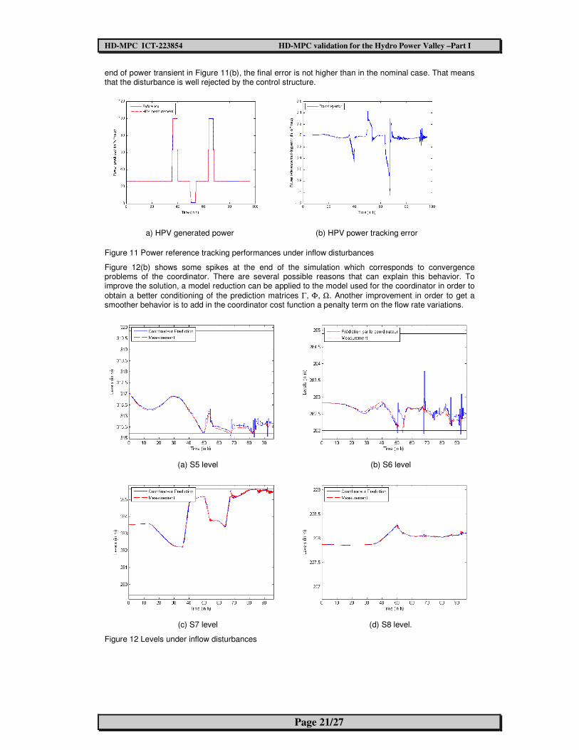
end of power transient in Figure 11(b), the final error is not higher than in the nominal case. That means that the disturbance is well rejected by the control structure.

a) HPV generated power (b) HPV power tracking error

Figure 11 Power reference tracking performances under inflow disturbances

Figure 12(b) shows some spikes at the end of the simulation which corresponds to convergence problems of the coordinator. There are several possible reasons that can explain this behavior. To improve the solution, a model reduction can be applied to the model used for the coordinator in order to

obtain a better conditioning of the prediction matrices Γ, Φ, Ω. Another improvement in order to get a smoother behavior is to add in the coordinator cost function a penalty term on the flow rate variations.

(a) S5 level (b) S6 level

(c) S7 level (d) S8 level.

Figure 12 Levels under inflow disturbances


/27

4.3 Model reliability

The simulation results presented in this section have been obtained on distributed control architecture applied on the non-linear simulation system with a modified Strickler coefficient on the whole river.

Power reference tracking. Figure 13 illustrates control performances in power program tracking. Again, the power reference is well followed. However, there is a more important constant bias than in the two previous cases. That shows that the Strickler coefficient variation for the HPV reaches is not well modeled by the control structure, and above all by the linear model.

(a) HPV generated power (b) HPV power tracking error

Figure 13 : Power reference tracking performances with modified Strickler coefficient

Prediction uncertainties. Figure 14 shows a bias in coordinator levels prediction. This is due to a difference between HPV linearized model and modified non-linear one.



Figure 14 : Impact on reaches’ levels with modified Strickler coefficient


/27

4.4 Validation Test with the Scicos/Mascaret model

The HD-MPC solution has been connected to the platform and the nominal scenario described in Section 4.1 has been simulated. The results are given in Figure 15 and Figure 16. Figure 15 shows that the power tracking is acceptable. Improvement should be made during the step changes, where the error can become significant during one or two sample time (60s). An analysis is under way to understand the cause of this transient error.


Figure 15 : Scicos/Mascaret Simulation results

0 10 20 30 40 50 60 70 80 90 100315

315.5

316

316.5

317

317.5

318

318.5

319

319.5

320

Time (in h)

Leve

ls (in

m)

Coordinateur Prediction

Measurement

0 10 20 30 40 50 60 70 80 90 100

281.5

282

282.5

283

283.5

284

284.5

285

Time (in h)

Leve

ls (in

m)

Prédiction par le coordinateur

Measurement


0 10 20 30 40 50 60 70 80 90 100259

260

261

262

263

264

265

266

Time (in h)

Leve

ls (in

m)


Measurement

0 10 20 30 40 50 60 70 80 90 100227

227.2

227.4

227.6

227.8

228

228.2

228.4

228.6

228.8

229

Time (in h)

Leve

ls (in

m)


Measurement


Figure 16 : Scicos/Mascaret Simulation results

Figure 16 shows that the reach levels are kept within their limits. As the constraints are soft, the levels


/27

can however go over or under these limits. This is the case for the reach of the subsystem S5 where the predicted level goes under the lower limit. The measurement does not follow the reference predicted by the coordinator, because the local controller makes a compromise between the power and level reference given by the coordinator. To improve the level control the weighting of the local problem can be tuned, but it will be at the expense of the power tracking. Another improvement can be obtained using a more accurate model in the coordinator.

4.5 Comparison with centralized MPC

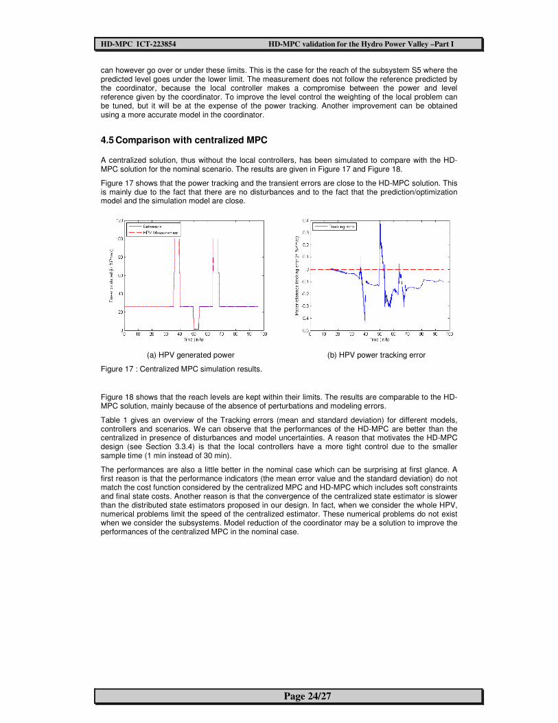
A centralized solution, thus without the local controllers, has been simulated to compare with the HD-MPC solution for the nominal scenario. The results are given in Figure 17 and Figure 18.

Figure 17 shows that the power tracking and the transient errors are close to the HD-MPC solution. This is mainly due to the fact that there are no disturbances and to the fact that the prediction/optimization model and the simulation model are close.


Figure 17 : Centralized MPC simulation results.

Figure 18 shows that the reach levels are kept within their limits. The results are comparable to the HD-MPC solution, mainly because of the absence of perturbations and modeling errors.

Table 1 gives an overview of the Tracking errors (mean and standard deviation) for different models, controllers and scenarios. We can observe that the performances of the HD-MPC are better than the centralized in presence of disturbances and model uncertainties. A reason that motivates the HD-MPC design (see Section 3.3.4) is that the local controllers have a more tight control due to the smaller sample time (1 min instead of 30 min).

The performances are also a little better in the nominal case which can be surprising at first glance. A first reason is that the performance indicators (the mean error value and the standard deviation) do not match the cost function considered by the centralized MPC and HD-MPC which includes soft constraints and final state costs. Another reason is that the convergence of the centralized state estimator is slower than the distributed state estimators proposed in our design. In fact, when we consider the whole HPV, numerical problems limit the speed of the centralized estimator. These numerical problems do not exist when we consider the subsystems. Model reduction of the coordinator may be a solution to improve the performances of the centralized MPC in the nominal case.


/27



Figure 18 : Centralized Simulation results

Mean Tracking Error [%] Centralized MPC HD-MPC

Nominal 0.10 0.08

Disturbance 0.16 0.07

Strickler 1.02 0.20

Nominal (Mascaret*) NA 0.20

Stand. Dev. Tracking Error [%] Centralized MPC HD-MPC

Nominal 0.08 0.07

Disturbance 0.25 0.13

Strickler 0.71 0.09

Nominal (Mascaret*) NA 0.34

* without the extreme errors due to sample time differences.

Table 1 : Comparison centralized MPC vs HD-MPC


/27

5 Conclusions

HPV optimal power reference tracking deals with current electricity production problems. Clean electricity production can be optimized by an optimal use of natural resources. Model predictive control can improve water management by using process evolution prediction models.

During this study, a hierarchical distributed MPC architecture has been developed. First, a non-linear simulation model has been realized within the Matlab/Simulink environment. Then it has been decomposed and linearized for MPC control purposes. The centralized MPC architecture has been modified into a HD-MPC structure combining a long prediction horizon and a fast control algorithm.

The simulation results show that reliable power tracking is possible while respecting operating and environmental constraints. Validation tests have been achieved with the detailed non linear Mascaret/SciCos model, which show a good behavior. Moreover, the benefits of the MPC anticipation have been highlighted on a really difficult power program simulation case.

Future prospects

First of all, many simulation tests can still be done for example to analyze the effect of a communication loss between the coordinator and the local controller or of a turbine loss on the solutions provided by the coordinator. Reliability to such events will be better managed by the distributed architecture than a centralized one.

Some improvements have to be done in order to force the control algorithm to undergo a cautious behavior ensuring HPV future maneuverability for example by forcing the final levels to a reference far enough from the limit.

Some improvements can be done with respect to the Kalman filters and MPC controller tuning. The impact of each tuning parameter must be studied. Moreover, the possibility to add a centralized Kalman filter for the coordinator even in HD-MPC should also be analyzed.

Finally, model simplifications and modifications should be adopted in order to solve some state estimation problems in the coordinator. For example, applying a model reduction to the entire HPV model and adding a downstream level measurement on each plant could improve disturbances and state estimation.

Benefits

This study has laid the foundation of a deeper analysis of the HD-MPC architecture applied to HPV. Results show that it is efficient for power program tracking purposes. It has also shown the importance of the interactions prediction in the algorithm efficiency. Moreover these results have been obtained for an extreme power program, with a few measurements compared to what could be available on operated plants. It is promising for future developments.


/27

6 Bibliography

[1] D. Faille, F. Davelaar, F. Petrone, R. Scattolini, H. Scheu, and C. Savorgnan, Report on the Model and Open-Loop Simulation Results for the Hydro Power Valley, Project report, August 2010.

[2] D. Faille, Control Specification for Hydro Power Valleys, Project report, September 2009.

[3] J. Zarate Florez, J. J. Martinez, G. Besançon, and D. Faille, Explicit coordination for MPC-based distributed control with application to Hydro-Power Valleys, 2011.

[4] S. Hovland, Soft Constraints in Explicit Model Predictive Control, Master’s thesis, Norwegian University of Science and Technology, June 2004.

[5] M. D. Mesarovic, D. Macko, and Y. Takahara, Theory of Hierarchical, Multilevel, Systems, Academic Press, 1970.

[6] Paul Scherrer Institut, http://gabe.web.psi.ch/projects/externe_pol/index.htm, ExternE-Pol project description and results – September 1st 2011.

[7] F. Petrone, Model Predictive Control of a Hydro Power Valley, Master’s thesis, Politecnico di Milano, 2010.

[8] B. Picasso, C. Romani, and R. Scattolini, On the design of hierarchical control systems with MPC.

[9] C. Savorgnan and M. Diehl, Control benchmark of a Hydro Power Plant, Version 1, 2011.

[10] A. Kozma, H. Scheu, Report on new algorithms with guaranteed convergence to an optimum of the global system, at a high rate of convergence, and with intelligent hot-starting, March 1, 2011

[11] R. Scattolini Report on the final assessment of the methods for the definition of the control architecture and preliminary report on extended algorithms coping with structural constraints, changes, and multi-level models, August 31, 2009

[12] F.V. Arroyave, L.D. Baskar, D. De Vito, B. De Schutter, J. Espinosa Oviedo, J.F. Garcia, A. Marquez, B. Picasso, R. Scattolini, A.N. Tarau, Final report on the results regarding multi-level models and architectures for hierarchical and distributed MPC, February 28, 2010

[13] I. Alvarado, D. Limon, D. Munoz de la Pena, J.M. Maestre, R.R. Negenborn, F. Valencia, H. Scheu, M.A. Ridao, B. De Schutter, J. Espinosa, W. Marquardt, A comparative analysis of distributed MPC techniques applied to the HD-MPC four-tank benchmark, 2010

SEVENTH FRAMEWORK PROGRAMME THEME – ICT … · HD-MPC ICT-223854 HD-MPC validation for the Hydro...

Documents

Transcript of SEVENTH FRAMEWORK PROGRAMME THEME – ICT … · HD-MPC ICT-223854 HD-MPC validation for the Hydro...