SETUP AND APPLICATION OF A

DIPLOMARBEIT:

SETUP AND APPLICATION OF A

SCANNING ION CONDUCTANCE M ICROSCOPE

Ausgefuhrt am Institut fur

Verfahrenstechnik, Umwelttechnik und

Techn. Biowissenschaften

der Technischen Universitat Wien

unter der Anleitung von Prof. Dr. Frank Rattay

durch

Stefan Schraml

Schlossgasse 2/1/9

A-1050 Wien

email: [email protected]

Vienna, November 5, 2003

3

Zusammenfassung

Ein Rasterionenleitungsmikroskop (Scanning Ion Conductance Microscope – SICM)

wurde aufgebaut und in Betrieb genommen. Das Rasterionenleitungsmikroskop

wurde aus einer konventionellen Patch-clamp Meßeinrichtung in Zusammenarbeit

mit einem Mikropositionierungssystem konstruiert. Die Patch-clamp Pipette wird

als Sonde verwendet. Die Sonde misst Ionenstrome so dass wahrend des Meßvor-

ganges kein physischer Kontakt mit der Probe stattfindet.

Das Mikroskop visualisiert stark unregelmaßige Oberflachen auf nicht-destruk-

tive und verformungsfreie Art und produziert dreidimensionale Bilder der Probe.

Im Gegensatz zu anderen Mikroskopen bietet das Rasterionenleitungsmikroskop

den Vorteil lebende Zellen in ihrer naturlichen Umgebung abbilden zu konnen ohne

sie beschadigen oder abtoten zu mussen.

In Pisa wurde in Kooperation mit Prof. Dr. Mario Pellegrino (Dipartimento

di Fisiologia e Biochimica, University of Pisa), Prof. Dr. Donatella Petracchi und

Prof. Dr. Cesare Ascoli, (Institute of Biophysics, National Research Council Italy)

ein Prototyp gebaut und getestet. Eine Erweiterte Version wurde amInstitut fur

Verfahrenstechnik, Umwelttechnik und Techn. Biowissenschaftenan derTechnis-

chen Universitat Wieninstalliert. Als Beispielapplikation wurden Aufnahmen von

roten Blutkorperchen gemacht.

4

Abstract

A Scanning Ion Conductance Microscope (SICM) for research and educational

purposes has been constructed and put in operation. The Scanning Ion Conduc-

tance Microscope is constructed from conventional patch clamp devices in con-

junction with a micro-positioning system. The patch clamp pipette is used as a

probe. The probe senses ion currents hence no physical contact to the specimen

takes place during scan.

The microscope visualizes highly irregular surfaces in a non-destructive and

deformation-free way and produces three-dimensional pictures of the specimen.

As opposed to other kinds of technical microscopes the Scanning Ion Conductance

Microscope provides the advantage of the ability to visualize living cells in their

natural environment without the need to damage or kill them.

A prototype has been built and tested in Pisa in cooperation with Prof. Dr.

Mario Pellegrino of theDipartimento di Fisiologia e Biochimica (University of

Pisa)and with Prof. Dr. Donatella Petracchi and Prof. Dr. Cesare Ascoli,Institute

of Biophysics (National Research Council Italy). An advanced version has been

installed at theInstitute of Chemical Engineering (Technical University of Vienna).

As example application pictures of red blood cells have been taken.

5

Acknowledgments

This work was supported by Prof. Dr. Frank Rattay, Dr. Ille Gebeshuber and Prof.

Dr. Helmut Stachelberger at the Technical University of Vienna and by Dr. Do-

natella Petracchi, Dr. Cesare Ascoli and Prof. Dr. Mario Pellegrini at the Diparti-

mento di Fisiologia e Biochimica ”G.Moruzzi” in Pisa.

Statement

I hereby certify that the work presented in this diploma thesis is my own and that

work performed by others is cited.

Ich versichere, diese Arbeit selbststandig verfasst, andere als die angegebenen

Quellen und Hilfsmittel nicht benutzt und mich auch sonst keiner unerlaubten

Hilfsmittel bedient zu haben.

Vienna, November 5, 2003

Stefan Schraml

6

“This equipment came from diverse technological epochs and had been smuggled

into this, the Outer Kingdom, from a variety of sources, but all of it contributed

to the same purpose: It surveyed the microscopic world through X-ray diffraction,

electron microscopy, and direct nanoscale probing, and synthesized all of the re-

sulting information into a single three-dimensional view.

If Hackworth had been doing this at work, he would already be finished, but

Dr. X´s system was a sort of polish democracy requiring full consent of all par-

ticipants, elicited one subsystem at a time. Dr. X and his assistants would gather

around whichever subsystem was believed to be farthest out of line and shout at

each other in a mixture of Shanghainese, Mandarin and technical English for a

while. Therapy included but was not limited to: turning things off, then on again;

picking them up a couple of inches and then dropping them; turning off nonessen-

tial appliances in this and other rooms; removing lids and wiggling circuit boards;

incense-burning; cable-wiggling; putting folded-up pieces of paper beneath table

legs; drinking cappuccino and sulking; invoking unseen powers; — and a similarly

diverse suite of troubleshooting techniques in the realm of software.” [Ste95]

CONTENTS 7

Contents

1 Introduction 10

2 Theory 13

2.1 Scanning probe microscopy. . . . . . . . . . . . . . . . . . . . . 13

2.1.1 Scanning tunnelling microscopy. . . . . . . . . . . . . . 15

2.1.2 Atomic force microscopy. . . . . . . . . . . . . . . . . . 17

2.1.3 Other techniques. . . . . . . . . . . . . . . . . . . . . . 19

2.2 Patch-clamp technique. . . . . . . . . . . . . . . . . . . . . . . 21

2.3 Scanning ion conductance microscopy. . . . . . . . . . . . . . . 24

3 Experimental setup 30

3.1 Optical microscope. . . . . . . . . . . . . . . . . . . . . . . . . 33

3.2 Micro-manipulator . . . . . . . . . . . . . . . . . . . . . . . . . 34

3.3 Piezo-actuator. . . . . . . . . . . . . . . . . . . . . . . . . . . . 34

3.4 Headstage. . . . . . . . . . . . . . . . . . . . . . . . . . . . . . 35

3.5 Pipette holder. . . . . . . . . . . . . . . . . . . . . . . . . . . . 36

3.6 Micropipette. . . . . . . . . . . . . . . . . . . . . . . . . . . . . 36

3.7 Piezo controller. . . . . . . . . . . . . . . . . . . . . . . . . . . 37

3.8 Patch-clamp amplifier. . . . . . . . . . . . . . . . . . . . . . . . 38

CONTENTS 8

3.9 Oscilloscope. . . . . . . . . . . . . . . . . . . . . . . . . . . . . 39

3.10 Function generator. . . . . . . . . . . . . . . . . . . . . . . . . 39

3.11 Vibration damping . . . . . . . . . . . . . . . . . . . . . . . . . 39

3.12 Data acquisition. . . . . . . . . . . . . . . . . . . . . . . . . . . 40

3.13 Faraday Cage. . . . . . . . . . . . . . . . . . . . . . . . . . . . 40

3.14 Pipette Puller. . . . . . . . . . . . . . . . . . . . . . . . . . . . 41

4 Software and mode of operation 42

5 Using the SICM 47

5.1 Preparations. . . . . . . . . . . . . . . . . . . . . . . . . . . . . 47

5.1.1 Pulling micropipettes. . . . . . . . . . . . . . . . . . . . 47

5.1.2 Electrodes. . . . . . . . . . . . . . . . . . . . . . . . . . 49

5.1.3 Preparing a sample. . . . . . . . . . . . . . . . . . . . . 50

5.1.4 Testing the EPC 7. . . . . . . . . . . . . . . . . . . . . . 51

5.1.5 Testing the EDA unit. . . . . . . . . . . . . . . . . . . . 54

5.1.6 Preparing the microscope. . . . . . . . . . . . . . . . . . 54

5.2 Obtaining data. . . . . . . . . . . . . . . . . . . . . . . . . . . . 56

5.2.1 Measuring the pipette resistance. . . . . . . . . . . . . . 57

5.2.2 Approaching the sample. . . . . . . . . . . . . . . . . . 58

5.2.3 Recording an approaching curve. . . . . . . . . . . . . . 59

5.2.4 Starting a scan. . . . . . . . . . . . . . . . . . . . . . . 60

5.2.5 Processing and visualizing the data. . . . . . . . . . . . 61

5.3 Performed tests. . . . . . . . . . . . . . . . . . . . . . . . . . . 62

5.3.1 Approaching curves. . . . . . . . . . . . . . . . . . . . 64

5.3.2 Scans. . . . . . . . . . . . . . . . . . . . . . . . . . . . 66

CONTENTS 9

6 Proposed improvements 69

7 Conclusion 71

List of abbreviations 73

List of figures 74

Bibliography 76

CHAPTER 1. INTRODUCTION 10

Chapter 1

Introduction

The principle of the scanning ion conductance microscope (SICM) was invented

at the University of Santa Barbara by the Hansma Group AFM Lab [Hea89]. It

belongs to the family of scanning probe microscopes and works with specimen in

conductive solution at room temperature and atmospheric pressure.

The SICM uses conventional patch clamp devices for the measurement of ion

currents. The patch-clamp pipette is used as scanning probe. Due to the functional

principle of sensing ion currents no physical contact to the sample is necessary

during the scan. The movement of the scanning probe is accomplished by a piezo

actuator.

The microscope is able to visualize highly irregular surfaces in a non-destructive

and deformation-free way and produces three-dimensional pictures of the speci-

men. As opposed to other kinds of technical microscopes the SICM provides the

advantage of the ability to visualize living cells in their natural environment with-

out the need to damage or kill them. The specimen needs only enough fixation to

prevent them from drifting. Even dynamical processes on the cell surface can be

measured.

Applications of the SICM range from corrosion research, quality control and

examination of technical and biological membranes to specialized medical and

pharmaceutical topics regarding cell and ion-channel behavior.

The SICM is an excellent research tool with an array of promising applica-

tions in the fields of Biology, Micro- and Nanotechnology. At the present time


Figure 1.1: A scan of red blood cells with applied median filter

no commercial SICMs are available. The motivation for this thesis was to show

that a reliable working SICM can be constructed at reasonable cost and that actual

research work can be done with this SICM.

Therefore the scope of this thesis was to construct a working SICM. This device

should be set up with special regard to low cost-components and flexible experi-

mentation. Test scans of various surfaces and in particular of cell membranes have

been taken as proof of concept. An example scan of red blood cells is shown in

Fig.1.1. The image range for this scan is 60×60µm.


The SICM we constructed excels in its working area which is up to 80×80µm

at resolutions down to 20 nm. The resolution depends directly on the opening diam-

eter of the micro-pipette. The control circuit of the piezo micro-positioning system

is working in closed loop mode to compensate hysteresis effects of the piezo ele-

ment. Special precautions have been taken in the scanning sequence to prevent the

micropipette tip from breaking. Instrumentation methods and measurement algo-

rithms have been optimized in order to scan biological surfaces in reasonable time.

In chapter2 the theory and modes of operation of different kinds of scanning

probe microscopes are described. The basics of the patch-clamp technique are

explained and the principles of the SICM is presented.

The experimental setup developed in this thesis is described in chapter3. The

numerous items constituting the SICM are individually explained.

Control of the measuring sequences is carried out by the software. The used

algorithms, functions and controlling structures are described in chapter4.

Often used methods and work steps necessary for measurement with the SICM

are introduced in chapter 5. Detailed instructions for the handling of the SICM and

some obtained pictures can also be found in this chapter.

To take the SICM from its present prototype status to a fully fledged research

tool some enhancements have to be done. These are described in chapter 6.

CHAPTER 2. THEORY 13

Chapter 2

Theory

2.1 Scanning probe microscopy

While scanning probe microscopes (SPMs) vary widely in application and reso-

lution the basic principle is the same: SPMs use a probe which senses a physical

quantity an a very small length scale. According to the type of SPM the measured

quantity changes in a significant way when the probe approaches the samples sur-

face. This quantity is either recorded directly (in so-called constant height mode)

or used to adjust the vertical position of the probe above the sample surface while

scanning [Mea88]. Usually either the sample or the probe is moved by a piezo

actuator.

Since SPMs does not use optics there are no lenses and the resolution of the

SPM is generally dependent from the tip size and the length scale at which the

measured quantity is changing.

Most SPM´s can operate in two modes:constant currentor constant height

mode.

In constant current modethe probe is moved at a specified distance above the

surface thus following the topology of the specimen. The height dependent signal

(current) is kept constant this way. Since the height has to be controlled constant

current scans are slower than constant height scans. In constant current mode the

scanned surface may be somewhat irregular.


In constant height modethe height of the tip over the surface is fixed. The

changes in the signal are recorded and an image of the surface is derived from

them. This means that the irregularities of the scanned surface may not exceed the

constant height. In return constant height scans are very fast as there is nothing to

be controlled.

Depending on the measured quantity and the corresponding requisites to probe

and sample every scanning probe microscope is suitable for more or less special-

ized applications. Since the Scanning Tunnelling Microscope was invented, many

applications and different types of SPMs have been developed. Some of the most

important types of SPMs will be discussed in the following chapter.


A c t u a t o r

S a m p l eC o n d u c t i v e L a y e r

V a c u u m

T u n n e l c u r r e n t

T u n g s t e n t i p

Figure 2.1: Principle of a STM

2.1.1 Scanning tunnelling microscopy

The invention of the Scanning Tunnelling Microscope (STM) in 1982 has intro-

duced new ways of examining surfaces with resolutions down to atomic levels

[Bea82]. For the first time it was possible to reach atomic resolutions without the

physical barriers of diffraction. A detailed review can be found at [BR87].

The STM works according to the following principle: The scanning probe is

a metallic tip (usually made from tungsten wire) biased with a voltage against a

conducting sample surface. The voltage induces a small current (approximately

1nA) between tip and the surface. This current is called Tunnelling current. It

stems from the non-vanishing probability density of electrons in the immediate

vicinity of the sample surface.

To detect this current the whole measurement is usually carried out in ultra

high vacuum (UHV). The vacuum also prevents contamination of the surface. The

current depends on the distance between tip and surface. Non-vacuum STMs exist

but are only utilized for special purposes.


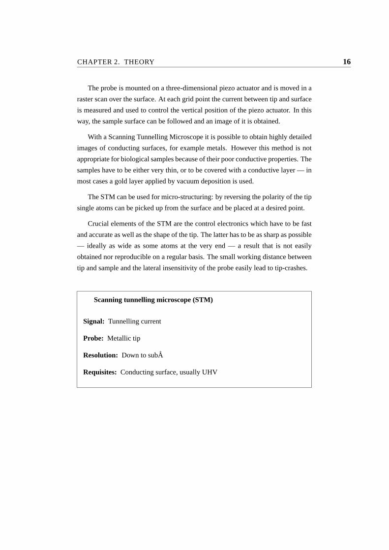
The probe is mounted on a three-dimensional piezo actuator and is moved in a

raster scan over the surface. At each grid point the current between tip and surface

is measured and used to control the vertical position of the piezo actuator. In this

way, the sample surface can be followed and an image of it is obtained.

With a Scanning Tunnelling Microscope it is possible to obtain highly detailed

images of conducting surfaces, for example metals. However this method is not

appropriate for biological samples because of their poor conductive properties. The

samples have to be either very thin, or to be covered with a conductive layer — in

most cases a gold layer applied by vacuum deposition is used.

The STM can be used for micro-structuring: by reversing the polarity of the tip

single atoms can be picked up from the surface and be placed at a desired point.

Crucial elements of the STM are the control electronics which have to be fast

and accurate as well as the shape of the tip. The latter has to be as sharp as possible

— ideally as wide as some atoms at the very end — a result that is not easily

obtained nor reproducible on a regular basis. The small working distance between

tip and sample and the lateral insensitivity of the probe easily lead to tip-crashes.

Scanning tunnelling microscope (STM)

Signal: Tunnelling current

Probe: Metallic tip

Resolution: Down to subA

Requisites: Conducting surface, usually UHV


L i g h t S e n s o r L a s e r

L a s e r b e a m

S a m p l eT i p L e v e r

A c t u a t o r

Figure 2.2: Principle of a AFM

2.1.2 Atomic force microscopy

The Atomic Force Microscope (AFM) operates by measuring attractive or repul-

sive forces between the tip and the sample [BQG86]. In its repulsivecontact mode

a tip at the end of a flexible leaf spring or “cantilever” touches the sample.

As a raster-scan drags the tip over the sample, a detection apparatus measures

the vertical deflection of the cantilever, which indicates the local sample height.

Thus, in contact mode the AFM measures hard-sphere repulsion forces between

the tip and sample. In most cases, the detection apparatus consists of a laser beam

which is reflected at the cantilever. This beam acts as a contact-free pointer and its

deflection is detected by a light-sensor [Aea88].

In so-callednon-contact mode, the AFM derives topographic images from mea-

surements of attractive forces. The lever is exited with vibration at its resonance

frequency. When the tip is now attracted by near atoms (without touching them),

the vibration frequency changes. With this method it is possible to achieve sub-

atomic resolution. This mode does not allow the imaging of samples immersed in

liquid.


Yet another possibility is theAttractive Mode Force Microscope(AMFM).

When the probe tip is brought within a distance of 2 nm to 20 nm of a sample,

the tip is pulled towards the sample by van der Waals forces as well as by the

surface tension created by water molecules that condense between tip and sample.

Monitoring the attractive force produces a topographic map of the samples surface.

Atomic Force Microscopes can achieve a resolution of 10 pm, and unlike elec-

tron microscopes, these devices are able to image samples in air and in liquids

[MDH87] [Dea89].

The cantilever of an AFM has to be very flexible in order to exert lower down-

ward forces on the sample. On the other hand he resonance frequency of a AFM

cantilever should be high to enable fast scans. Both requirements can be fulfilled

by using cantilevers with a very small mass. Commercial vendors manufacture al-

most all AFM cantilevers and tips by microlithography processes similar to those

used to make computer chips.

In principle, AFM resembles the record player as well as the stylus profilome-

ter. However, AFM incorporates a number of refinements that enable it to achieve

atomic- or even sub-atomic scale resolution. For high resolutions the AFM has to

operate in UHV since dust and condensed water would interfere with the measure-

ment. AFMs are highly developed and commercially available.

Atomic force microscope (AFM)

Signal: Deflection of a cantilever

Probe: sharp tip on a flexible cantilever

Resolution: 10 pm

Requisites: Regular surface, UHV for high resolutions


2.1.3 Other techniques

Friction force microscope (FFM): The friction between a thin tip (the probe) and

the specimen surface is measured. The goal is to investigate friction on an

atomic scale. Usually modified AFMs where the torque of the tip is mea-

sured are used for this method.

Magnetic force microscope (MFM): [AP03] The construction is similar to a AFM

but the tip is coated by a magnetic thin film. MFMs are used to investigate

the magnetic domain structure with resolutions from 25–100 nm . The MFM

has been especially useful in studying magnetic recording devices such as

computer hard disks.

A very important problem in MFM is the separation of the magnetic image

and the topography. To solve this problem the magnetic measurements are

executed by means of two-pass method. In the first pass the topography is

determined in contact or semi-contact mode. In the second pass the can-

tilever is lifted to a specified height and scanned using the stored topography

(without the feedback). As a result the tip-sample separation during second

pass is kept constant. During the second pass the short-range van der Waals

force vanishes and the cantilever is affected by long-range magnetic force

only. Both the height-image and the magnetic image are obtained simulta-

neously with this method.

Electrostatic force microscope (EFM): In this microscope the metallic scanning

tip is charged electrically. The electrostatic forces between the charged tip

and electric charges on a surface are measured.

Scanning thermal microscope (SThM): This technique adds a highly miniatur-

ized thermistor to the AFM tip. SthMs are used for the characterization of

thermal gradients with 200 nm spatial resolution and 0.2K temperature

resolution [WW86].

Optical absorption microscope : It can be used to determine the chemical com-

position of a surface by using absorption spectroscopy. Shining a laser on

a sample heats up some atoms more than others and the temperature differ-

ences can be detected by a thermal microscope. Varying the wavelength of

the laser gives an absorption spectrum of the surface which in turn gives its


chemical composition. Resolutions down to 1 nm are possible, making it

possible to record the spectrum of a single molecule.

Scanning acoustic microscope (SAM):A project to develop a scanning acoustic

microscope actually predates the invention of the STM. Stanford researchers

have been imaging samples with sound, using a sonar-like technique. Res-

olutions of 40 nm have been obtained by using sound frequencies of 8 GHz

and cooling the sample to less than 0.5K in liquid helium.

Molecular dip-stick microscope : An application of the Atomic Force Micro-

scope, the molecular dip-stick illustrates the versatility of the new micro-

scopes. To measure the thickness of very thin lubricant films, the tip of an

AFM is lowered into the lubricant like a dip-stick. The tip feels a strong

attractive force from surface tension when it touches the lubricant and then

a repulsive force when it reaches the underlying surface. The molecular dip-

stick can determine the depth of a lubricant to an accuracy of 5A.

Shear force microscope (SHFM): [Kam95] The probe is mounted on a piezo-

electric actuator which drives the probe at a frequency close to one of its

resonant modes. The tip is mounted in such a way that its direction of vi-

bration is parallel to the sample surface. As the probe is moved into close

proximity of the sample, the amplitude of oscillation decreases due to damp-

ing from the van der Waals interactions. Sub-Angstrom changes in the tip

to sample separation can be detected in the feedback signal. This signal is

generated by focusing a laser at the tip and measuring the intensity of the

diffraction image.

Scanning near-Field optical microscope (SNOM) :An optical microscope is not

able to give a resolution better than about 200 nm, or about half the wave-

length of visible light. This limit can be circumvented by using a near-field

technique where either the light source or the detector is smaller than wave-

length the of the light and is brought very close to the specimen. Using this

method resolutions about 40 nm can be achieved.


C e l l M e m b r a n e

M i c r o i p e t t e

I o n C h a n n e l s

Figure 2.3: Patch-clamp

2.2 Patch-clamp technique

Patch-clamping is an electro-physiological method used to monitor the ion current

of single ion-channels in the membranes of living cells [NS92]. These currents

are so small that they cannot be easily detected due to the background noise in the

measurement setup. The dimension of these current pulses is in the pico-ampere

range. To isolate the signal from noise, a glass tube, pulled to a diameter of ap-

proximately 1µm is brought near the cell surface. Detailed information regarding

patch clamp pipettes is given in chapter3.6.

By applying some negative pressure on the pipette it is likely that the cell is

sucked to the pipette opening. Thereby the concealed area (the so-calledpatch)

of the cell membrane is electrically isolated from the surrounding solution. In this

way the influence of electrical background noise is blocked by the pipette (see


a . ) b . )

c . ) d . )

Figure 2.4: Cell configurations:

a.) Cell-attached b.) Inside-out

c.) Whole-Cell d.) Outside-out

Fig.2.3).

This phenomenon is called the forming of a gigaseal (the resistance is usually

greater then 1 GΩ). The electrical properties of the ion channels in the patch can be

investigated. If ion-channel density and pipette opening diameter are appropriate,

it is possible to record the ion current from single channels.

When forming a gigaseal, the cell membrane sticks tightly to the glass pipette

thus providing electrical isolation to the patch. Through various kinds of manipu-

lation different cell-configurations can be achieved without de-attaching the patch.

In this way not only single channels can be measured in the so calledcell-attached

configuration, but it is also possible to break the patch to get access to the cy-

toplasm of the cell. Thiswhole-cell configurationcorresponds to a conventional

intra-cellular recording.

Furthermore it is possible to measure the properties of the patches with the

cytoplasmic side directed to the bath or to the pipette (inside-outor outside-in

configuration). See Fig.2.4for illustrations.


A variant is the loose-patch method: hereby there is no gigaseal formed be-

tween the pipette and the cell. In this case a lot of noise is introduced to the mea-

surement and it gets hard to identify the signal.

The patch-clamp method is widely used in laboratories to examine the behavior

of Ion channels and transmitter-receptors. Today patch-clamping is probably the

most widely used electro-physiological method for the investigation of ion chan-

nels. In 1991 the Nobel price in physiology was granted to Erwin Neher and Bert

Sakman for developing this method.


B a t h s o l u t i o n

M i c r o p i p e t t eE l e c t r o d e

S a m p l eI o n c u r r e n t

B a t h e l e c t r o d e

A c t u a t o r

Figure 2.5: Principle of a SICM

2.3 Scanning ion conductance microscopy

A Scanning Ion Conductance Microscope (SICM) is a Scanning Probe Microscope

which has been developed to image the topography of non-conducting surfaces that

are covered with electrolytes at atmospheric pressure [Hea89].

The scanning tip of a SICM consists of a pulled out glass tube (called micro-

pipette) filled with electrolyte and containing an electrode. Similar pipettes are

used in the patch-clamp technique. A difference to patch clamp pipettes is the

opening diameter of the tip which should be smaller than for patch-clamp applica-

tions. As will be shown below the longitudinal resolution of the SICM corresponds

directly to the opening diameter of the pipette.

The imaging technique of the SICM is based on the measurement of the ion

current between two electrodes. One electrode is placed inside of the pipette, the

other electrode is located in the bath solution (See Fig.2.5). To avoid electrical drift

the bath solution and the solution inside of the pipette should be the same.


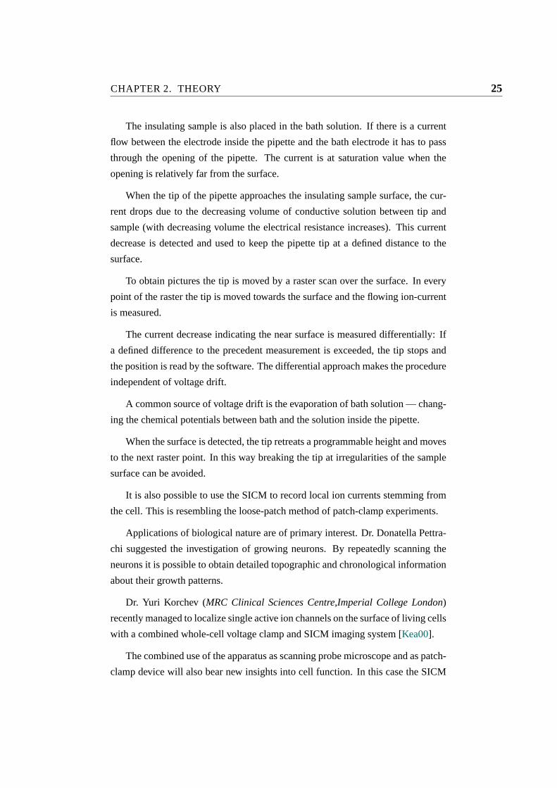
The insulating sample is also placed in the bath solution. If there is a current

flow between the electrode inside the pipette and the bath electrode it has to pass

through the opening of the pipette. The current is at saturation value when the

opening is relatively far from the surface.

When the tip of the pipette approaches the insulating sample surface, the cur-

rent drops due to the decreasing volume of conductive solution between tip and

sample (with decreasing volume the electrical resistance increases). This current

decrease is detected and used to keep the pipette tip at a defined distance to the

surface.

To obtain pictures the tip is moved by a raster scan over the surface. In every

point of the raster the tip is moved towards the surface and the flowing ion-current

is measured.

The current decrease indicating the near surface is measured differentially: If

a defined difference to the precedent measurement is exceeded, the tip stops and

the position is read by the software. The differential approach makes the procedure

independent of voltage drift.

A common source of voltage drift is the evaporation of bath solution — chang-

ing the chemical potentials between bath and the solution inside the pipette.

When the surface is detected, the tip retreats a programmable height and moves

to the next raster point. In this way breaking the tip at irregularities of the sample

surface can be avoided.

It is also possible to use the SICM to record local ion currents stemming from

the cell. This is resembling the loose-patch method of patch-clamp experiments.

Applications of biological nature are of primary interest. Dr. Donatella Pettra-

chi suggested the investigation of growing neurons. By repeatedly scanning the

neurons it is possible to obtain detailed topographic and chronological information

about their growth patterns.

Dr. Yuri Korchev (MRC Clinical Sciences Centre,Imperial College London)

recently managed to localize single active ion channels on the surface of living cells

with a combined whole-cell voltage clamp and SICM imaging system [Kea00].

The combined use of the apparatus as scanning probe microscope and as patch-

clamp device will also bear new insights into cell function. In this case the SICM


is used to localize specific ion channels. The pipette is then moved to these ion

channels and is used to measure their properties with the patch-clamp technique.

In medical terms research on matters like cell signalling and ion transport reg-

ulation will help to understand diseases such as cystic fibrosis, and how cardiomy-

ocytes are preserved during metabolic stresses such as hypoxia and ischaemia.

Other possible application possibilities are in the field of micro-structuring. It

should be possible to use the SICM for galvanic or chemical deposition. This could

be of special interest when trying to interface to cells or as additional method to

established micro-structuring procedures.

Since the occurring currents are in the nano-ampere range we use a patch-clamp

amplifier to detect them. The electrodes have to be of second order to measure ion

currents. To archive that, we put silver wire in chlorine-bleach overnight. On the

next day the silver wire is coated with a layer of AgCl.

The assumption that the lateral resolution of the SICM depends directly on the

opening diameter leads to the question how to calculate the height dependence of

the current as function of the geometrical properties of the pipette. The model from

the diploma thesis of E. Schwab [Sch90] was used to calculate the current when

approaching the sample surface.

In this model, the total resistance of the pipette is composed of a height-dependent

partRH between pipette tip and sample surface and an constant part given by the

ion-conductible liquid inside the frustum of the tip. The remaining resistance of

the bath solution is neglected in this model.

The resistanceR is in general proportional to lengthL and inversely propor-

tional to cross-sectionA and conductivityκ:

R=L

Aκ(2.1)

Thus, applied to the resistances of the frustumRF (with the pipette diameterrp

and the inner diameterr i) and the hollow cylinderRH (with the outer diameterro

and the heighth) :

RF =Lk

rpr iπκ(2.2)


r ir o

r p

L k

h

R F

R H

Figure 2.6: Model of a micro-pipette tip

RH =ln( ro

r i)

2πhκ(2.3)

Giving a total resistanceRT :

RT = RK +RH =UI

(2.4)

And resolved for the currentI :

I =Uκπ

Lkrpr i

+ln( ro

ri)

2h

(2.5)

When the tip is far away from the surface (h→ ∞) the so-called saturation

current (Isat) is flowing:

Isat = limh→∞

UκπLk

rpr i+

ln( rori

)2h

=Uκπ

Lkrpr i

(2.6)


To get a usable quantity the current is normalized to the saturation currentIsat:

IIsat

=1

1+ln( ro

ri)rpr i

2Lkh

(2.7)

The normalized ion current is only dependent on the geometrical properties of

the pipette and the heighth above the surface.

From this theoretical considerations some information about the ideal geometry

of the pipette can be derived. When measuring ion currents it is advantageous when

the current decrease begins at a greater distance above the specimen surface. This

should prevent the tip from crashing into the sample. This means for pipettes used

in the SICM that the electrode has to be near the opening — the frustum has to

be as short as possible. Furthermore the wall thickness of the pipette should be

large. With these premises the influence of the height-dependent resistanceRh is

dominant. See chapter3.6for details on micro-pipettes.

Equation 2.6 also gives us a possibility to estimate the opening diameter from

the measured resistance. WithUIsat

= Rpip = Lkrpr iκπ we obtain to:

r i =Lk

Rpiprpκπ(2.8)

With the knowledge ofRpip, rp andκ we can estimate the frustum lengthLk and

are able to calculate the opening diameter. The step-wideness for scans can only

be set to a good value if we have an estimation for the opening diameter.

A result of this computation is shown in Fig.2.7. A calculated and a measured

approaching curve are displayed. The geometric properties of the pipette have been

estimated and applied to the model calculation. The stated simple model seems to

reproduce the behavior of the approaching tip very well.


Figure 2.7: Calculated and measured approaching curves

(the spike at 2200 nm is a measuring artifact)

Scanning Ion Conductance Microscope (SICM)

Signal: Ion current

Probe: Micro-pipette

Resolution: About 20 nm

Requisites: Non-conducting sample in conductive liquid

Typical Applications: Visualization of living cells

CHAPTER 3. EXPERIMENTAL SETUP 30

Chapter 3

Experimental setup

The most important consideration in the design process was to keep the setup flex-

ible. The SICM therefor consists of two parts.

The SICMscanning head(Fig.3.1) is designed to be easily detachable from

any optical microscope and also works without any optical microscope at all. The

scanning head consists of the micro-manipulator holding the piezo actuator. Elec-

trically, the pre-amplifier is the most sensitive part of the setup. To keep signal

paths short the pre-amplifier is directly holding the pipette and is mounted on the

piezo actuator.

The SICM pre-amplifier could also be exchanged for the probe head of another

type of SPM. By utilizing the head as moving part (as opposed most other working

SICMs) we have plenty of room left on the stage of the optical microscope. This

free space can be used for a perfusion bath or another micro-manipulator – devices

that are necessary when doing complex experiments with cells. The compact build

of the micro-manipulator is important to reduce mechanical vibration.

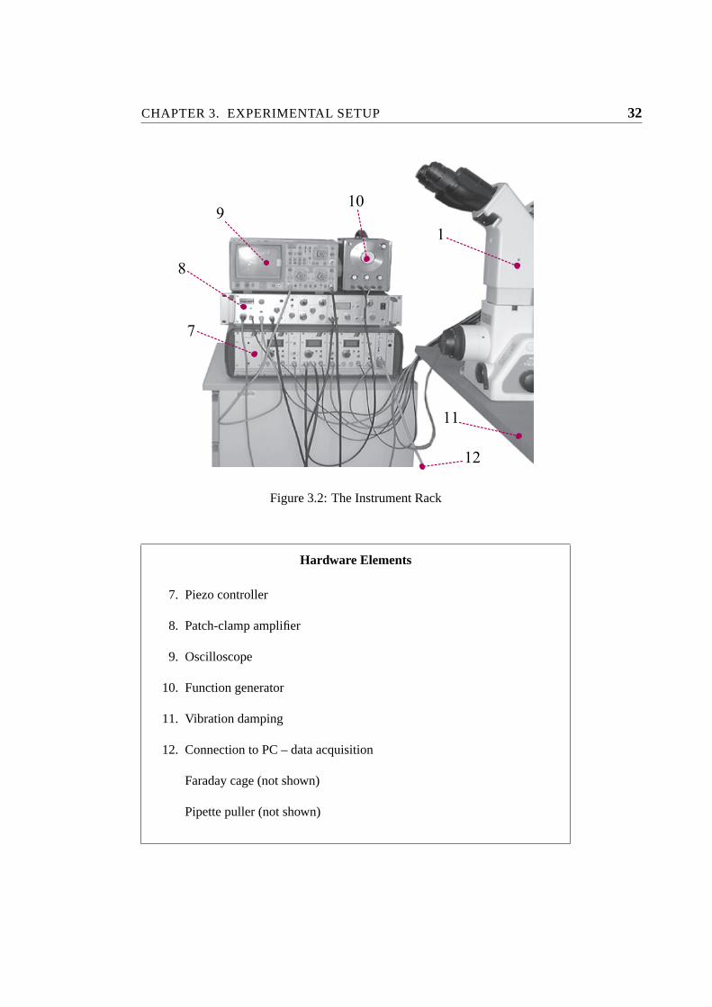
The instrument rack(Fig.3.2) holds the controlling devices. It is mechanically

separated from the optical microscope and the scanning head to prevent vibration.

The only connection consists of various cables, these are fixed to the vibration

damping steel plate. The instrument rack is placed on a trolley for more mobility.

A good working place should be free of mechanical vibration and acoustic

noise (e.g. slamming doors) as well as of electrical noise (especially on the ground–

line).


23

1 a

456 1 b

1 c

Figure 3.1: The Scanning Head of the SICM

Hardware Elements

1. (a) Optical microscope

(b) Object table

(c) Condenser

2. Micro-manipulator

3. Piezo-actuator

4. Headstage

5. Pipette holder

6. Micropipette


7

8

9 1 01

1 1

1 2

Figure 3.2: The Instrument Rack

Hardware Elements

7. Piezo controller

8. Patch-clamp amplifier

9. Oscilloscope

10. Function generator

11. Vibration damping

12. Connection to PC – data acquisition

Faraday cage (not shown)

Pipette puller (not shown)


3.1 Optical microscope

The purpose of the optical microscope is to aim the pipette tip to the target area.

To scan the specimen access from above is required. The optical part of normal

microscopes is therefore in the way so the most important criterium is that the

microscope is an inverted microscope. For the same reason the condenser of the

microscope should have a long working distance. Problems arise when trying to get

good picture quality: It is necessary to use objectives with a high numeric aperture.

This in turn requires a short working distance of the condenser. For these reasons

it is not possible to acquire optimal pictures when the SICM head is mounted on

the microscope.

A Nikon Eclipse TE300 inverted microscope is used for this thesis. This mi-

croscope offers professional optical properties and can be equipped with phase-

contrast or Nomarsky interference contrast devices, which will come handy when

working with cells.

Phase-contrast microscopy is a contrast-enhancing optical technique that can be

utilized to produce high-contrast images of transparent specimens, such as living

cells. Transparent structures may be visualized in phase microscopy by producing

contrast from refractive index inhomogeneities in the sample rather than from light

absorption inhomogeneities. Contrast is obtained by converting phase changes into

amplitude changes. Phase microscopy is well suited to studies of living tissue as

samples do not have to be fixed and stained in order for internal structure to become

visible.

Nomarsky microscopy, also called differential interference contrast (DIC) mi-

croscopy is a modification of phase microscopy. The technique essentially acts as

a high-pass filter that emphasizes edges and lines. Out-of-focus refractive index

changes will be blurred and have a shallow spatial gradient in the focal plane, they

will therefore not contribute much to the contrast of the image.

The condenser stand of the microscope can be tilted backwards which gives

additional room at the cost of good lightning.


3.2 Micro-manipulator

The micro-manipulator is mounted on the stage of the microscope. The manipu-

lator is used for rough positioning of the pipette and to place it near the sample

surface. The models usually used for patch clamping purposes are not useable for

our application since they do not offer the required mechanical stability to mount

the heavy piezo-actuator.

The used model Newport M-461-XYZ is made of steel and shows no drift. Its

travel is 13 mm in every direction and it provides mounting possibilities for the

piezo-actuator. All three axes can be equipped with stepper-motors.

When lowering the scanning head turn the knob anti-clockwise. A turn of14

corresponds to a movement of 60µm.

3.3 Piezo-actuator

The whole raster scan is done by aTritor 3D 100SGpiezo element fromPiezosys-

tem Jena. This actuator is compact and provides excellent mechanical stability. It

offers up to 100µm motion in every direction (80µm in closed loop mode) and it

is equipped with an integrated strain gauge measurement system for overcoming

the effect of hysteresis. Resolution for controlling each axis is 12 bit which corre-

sponds to 20 nm (resolution can be enhanced by the use of a pull down resistor).

Inside the piezo element the actual position is measured by strain gauges which

provide data for a feedback loop that prevents the piezo element from drifting and

nullifies the hysteresis normally observed in piezo movement. This is automatically

done by the piezos controller when switched to closed loop.


3.4 Headstage

The headstage is mounted directly on the piezo actuator. Note that in our setup the

moving part is the micropipette and not the sample. This is unusual but has the

advantage that one can look at the sample through the optical microscope any time

even during scan. The headstage contains the sensitive amplifier that constitutes

the current–to–voltage converter, as well as components for injecting test signals

into that amplifier. The headstage is capable of changing its range according to the

performed experiment. For further information see the manual [HEK].

On one side of the pre-amplifier is a BNC connector which holds an ankle on

which the pipette-holder is mounted. Thus the pipette holder can be slightly tilted

to let light from the optical microscopes condenser pass and to have the shadow of

the tip in the view-field of the optical microscope for observation.

On top of the headstage a pin jack carries a high quality ground signal which is

useful for grounding the bath electrode or nearby shields. As bath electrode also a

AgCl covered silver wire is used. For this reason the bath electrode and the pipette

electrode should be produced in the same process to prevent them from having a

potential difference.

Note that the metal casing of the probe is also connected to the signal, and

thereforemust be insulated from the groundand thus, also from the piezo actu-

ator.

The MC-7 is an accessory to the headstage. it is used as a model circuit for

testing purposes. This circuit simulates an open pipette, a gigaseal or a whole–cell

configuration. When in use it gets plugged to the headstage instead of the pipette

holder.


3.5 Pipette holder

Figure 3.3: The pipette holder and a

pipette

The holder (shown in Fig.3.3) is

provided with the patch clamp am-

plifier. It consist of Teflon and

polycarbonate and has a small

pipe leading out sideways to ap-

ply pressure to the pipette. This

pipe is needed when doing patch

clamp experiments to apply neg-

ative pressure to the tip in order

to establish the gigaseal. In the

SICM Setup it is sometimes used

to apply positive pressure to the

tip when entering the bath solu-

tion to prevent the tip from getting

clogged by debris.

The pipette electrode has to be

welded to the contact centerpiece.

Mounting to the headstage occurs

over a BNC connector. For clean-

ing the pipette holder methanol is

used.

3.6 Micropipette

The pipettes are produced by pulling glass tubes in a device called pipette puller.

The pipette is characterized by its wall thickness, opening diameter and tip length.

See chapter2.3for some calculations.

Pipettes can be pulled of soft glass, borosilicate or aluminiumsilicate glass or

quartz glass. In section5.1.1a description of the actual pulling process will be

given.


Soft glass tubes tend to have huge opening diameters and are sometimes toxic

to cells. Quartz glass has a very high melting point only reachable with expensive

laser pullers but offers superior electrical properties. Laser pullers also allow for

the best process control and can produce the smallest opening diameters (about 30

nm) reproducible. Aluminiumsilicate glass also produces useable tips which are

slightly longer and a bit more fragile but offer a smaller opening diameter. with

the available puller the best results have been obtained by using borosilicate glass

tubes.

For patch clamp experiments it is usual to cover the pipettes with hydrophobic

substances like Sylgard to improve the electrical properties of the tip. It is also not

uncommon to heat-polish the tip in a so called micro-forge. This method leads to

more rounded tips. None of these procedures are necessary when using the tips in

the SICM.

Usually it is best to pull the tip fresh when it is used but it is possible to store

them dust free with a small amount of silica for several months. Still, the danger

of clogged tips leading to tip-crashes is increasing with storage time.

Most experiments for this project have been done with borosilicate tubes (di-

ameter: 1 mm, wall thickness: 0.3 mm) resulting in tips with opening diameters

between 150 nm and 400 nm. The used puller did not produce reproducible results.

With the aid of a good puller it should be possible to obtain opening diameters

down to 15 nm [CGL92].

An interesting approach is the use of micro-fabricated tips as described in

[PH91]. These are etched from silicon and offer an opening diameter of about

250 nm. The advantage is the high mechanical robustness allowing high-speed

scans.

3.7 Piezo controller

The amplifier system corresponding to the piezo actuator was also chosen from

Piezosystem Jenas product range. A modular system containing power amplifiers

and position control modules for all three channels (named ENV) as well as an

interface board (EDA2) is used. The interface board allows control of the piezo by


Figure 3.4: Scanning electron microscope image of a micropipette

a PC via a RS232 serial connection. A programmable microprocessor is also avail-

able in this unit and can be utilized for future enhancements. Detailed information

can be found in the manual [Pie]

It is also possible to apply a modulating control voltage signal directly to each

module. This feature is used to control the vertical movement when scanning a

surface.

3.8 Patch-clamp amplifier

The model used is a Heka EPC 7 [HEK]. This is a classic patch clamp amplifier

with a good signal to noise ratio. It can be used for a variety of experiments. The

device consists of the main amplifier and a pre-amplifier also called theheadstage

or probe.

The main unit contains the power supply, the signal processing electronics and

all of the controls. The EPC 7 offers an extremely wide bandwidth and the inte-


grated transient cancellation and series–compensation functions add to the versa-

tility of the amplifier. Another very useful feature is the SEARCH-mode which

keeps the current signal from drifting off-scale.

The EPC 7 also offers a manually adjustable constant current. When the unit

is switched to VOLTAGE CLAMP mode this feature can be used to generate a

dc signal as stimulus. A constant stimulus has the advantage of reduced artifacts

when the ion current is sampled. This drastically improves the accuracy of the

measurements and thus, the stability of the scanning process.

3.9 Oscilloscope

A two-channel digital oscilloscope is used for various measurements and for signal

visualization. This device is essential when tracking errors.

3.10 Function generator

This instrument is used mainly for testing purposes. It produces a square signal.

For most experiments a direct-voltage offset can be generated by the patch-clamp

amplifier. With adapted software signal-generation can also be done by the Com-

puter via the NI-DAQ data acquisition card (NI-DAQ).

3.11 Vibration damping

Since the tip-sample distance of the SICM is quite small vibration of the apparatus

has to be prevented. All parts of the construction are selected to be robust and

compact leading to high resonance frequencies.

The vibration damping system consists of a steel plate of 45 kg resting on four

tennis balls. The optical microscope holding the scanning head rests on this plate.

This setup is simple yet effective — operation of the microscope runs smoothly

despite the four track heavy traffic street running alongside our institute building.

A similar construction with squash balls has been described in [OR95].


Vibration sensibility test were also made. For these test the tip was held at 1µm

over a glass surface then typical vibration sources (heavy steps, knocking on the

table, slamming doors etc.) were applied. The only thing that caused the tip to

move noticeably was slamming the rooms door.

3.12 Data acquisition

The measured ion current is sampled to a computer running Matlab via a National

Instruments data acquisition card. The computer controls the piezo, detects the

drop in ion current and records the data for successional imaging and analysis.

The analog output of the data acquisition card also provides the voltage slope

that drives the piezo in vertical direction during scan. The piezo controller is con-

nected to the computer via a RS232 cable to the COM2 port of the PC. The lateral

movement of the piezo is controlled using this signal path.

The NI-DAQ data acquisition card provides 8 AD channels (inputs) and 2 DA

converters (analog outputs) as well as 24 Digital I/O lines. The resolution of the

converters 12 bit. Since currently one input for the measured current and one output

channel to drive the piezo is used there are enough resources for future enhance-

ments. In particular timed output of stimulation signal pulses should be done with

this card.

Process control is done with Matlab running on a P133 PC (Matlab uses this

computer to full load). The Systems has 128MB RAM and the installed OS is Win-

dows 98 SE. Windows 98 offers better timing and stability for real-time purposes

than its successors.

3.13 Faraday Cage

Since the measured signal is very small it can easily be distorted or overlayed by

electrical background noise. To optimize the signal-to-noise ratio the working area

is shielded by a removable faraday cage.

The most common noise sources — the 50 Hz hum radiated by the power

lines and high–frequency radiation from computers and monitors are eliminated


Figure 3.5: Narishige Pipette puller

by this shielding. The Faraday cage must be mechanically de-coupled from the

microscope to prevent vibration pick-up.

3.14 Pipette Puller

We used an puller from Narishige, model PD-5. It is a Brown-Flaming type hor-

izontal puller. Pipettes are heated by a platinum filament without current control.

The force is applied in two phases. The first pull is selectable in a range from 0–10

g. When a micro-switch is triggered by the shaft the second pull is initiated with a

adjustable force from 0–100g.

To adapt the PD-5 for the pulling of SICM-pipettes the filament had to be

changed. Still the pulled pipettes were not very reproducible.

The puller used in this thesis was donated by Prof. Dr. Graf (AKH Vienna).

Since it was needed by another research group it has not been available for the

latest months. Information on pipette-pullers in general can be found at section

5.1.1.

CHAPTER 4. SOFTWARE AND MODE OF OPERATION 42

Chapter 4

Software and mode of operation

In the following chapter the software operating the SICM will be discussed. The

functional principles of the SICM will also be outlined. The controlling software

is written in Matlab (V6R12). Matlab is well suited for testing and visualization

purposes.

As starting situation of a scan it is assumed that the pipette tip is placed in the

solution and in a range of max. 40µm above the specimen. When using the SICM

the piezo has to be initialized and then the tip has to be moved manually into an

appropriate position (see5.2). A constant voltage is generated by the EPC 7 as

signal. This voltage should be adjusted to a litte bit below 5 V.

Initialization of the SICM is done by evoking the routinesiniteda and

initdaq . For reset purposes thekill function can be used. After invoking

kill re-initialization is possible.

initeda: Initializes the piezo-controller by switching it to computer control and

moving the piezo to the starting position.

The program creates a global variables which contains the handle for the

serial port. Explanation of commands sent to this port can be found in [Pie].

initdaq: Initializes the data acquisition card. The analog input is now ready to

sample the pipette current. The analog output is controlling also the vertical

axis of the piezo and is also set to its starting position.


Here the global variablesai andao are defined. Those carry the handles for

the analog in- and output. The sample-rate is set to 1KHz for both channels

and a value according to a height of 40µm (the maximum height for the

vertical axis when) is set for the output channel.

This is done by the subfunctionmovez(var) . This function utilizes the

movement of the piezo by sending the according voltage to the analog out-

put. The parametervar is to be given inµm.

kill is a cleanup-routine. If something goes wrong and it is necessary to man-

ually interrupt a scan this program should be called afterwards to clean the

buffers and close all open instruments.

approach(startheight,Istopratio) The recording of anapproaching

curveis done by invoking the program

curve=approach(startheight,Istopratio) . The measured ap-

proaching curve is saved incurve . The parameterstartheight is to be

given inµm and specifies the starting height of the approach.

The piezo is moved down step by step and in every point an average of 20

samples is taken. For this movement the (slower) method of controlling the

piezo via the EDA-controller is used. An advantage is that the full range of

80µm on the vertical axis can be used with this method.

At the beginning of the measurement the saturation current is sampled (as an

average of 5×20 samples). The approach stops at an defined ratio between

actual current and saturation current (the parameterIstopratio ). When

stopped the tip is retreated from the surface and the obtained curve is dis-

played. This method delivers accurate absolute current values.

raster This routine is used for the actual raster scan of the surface. The param-

eters of the scan like x- and y-range, step-width etc. have to be changed in

the code accordingly to the experiments needs. The code for this function

is shown below. To start a scan set the parameters in the code and evoke

the function withmap=raster . The obtained data is saved in the variable

map.


function map=raster;% handle of the analog inputglobal ai

% parameters of the scanIstopratio=0.999;startheight=30;

xstep=0.25;ystep=0.25;xmin=0;xmax=10;ymin=0;ymax=10;tapheight=3;

% initializationline=[];map=[];height=startheight;x=xmin;y=ymin;movez(height)movea(1,x)movea(3,y);

% raster loopwhile y<ymax

while x<xmax and x>xmin% find the surfaceheight=probe(Istopratio);line=[line height];% retreat from surfaceheight=height+tapheight;movez(height);% move to the next stepx=x+xstep;movea(1,x);

end% next line% switch directionxstep=xstep*(-1)x=x+xstep;y=y+ystep;to the next linemovea(1,x);movea(3,y);% append line to mapmap=[map;line];line=[];

end% return to startposmovez(startheight)movea(1,xmin);movea(3,ymin);

%calculate number of elementsx=xmin:xstep:(xmax-xstep);y=ymin:ystep:(ymax-ystep);% show surface mapsurfl(x,y,map,[80 50])colormap(copper)shading interpxlabel(’x (m)’)ylabel(’y (m)’)zlabel(’z (m)’)view(120,30)

When scanning, the vertical piezo position is controlled by a voltage delivered

by the analog output of the NI-DAQ card. This method is much faster than the

step-by-step method used in theapproach function. The controlling voltage is

dropped in a slope, thus the pipette is moved towards the surface. While pipette


moves the output of the patch-clamp amplifier (the actual ion-current) is sampled

at 1 KHz and analyzed in realtime.

An average of 20 samples is taken and compared with the last measurement. If

the difference exceeds a defined ratio, the voltage slope is stopped and the position

of the tip is determined by the functionreadheight .

This method is very fast and sensitive. Since the result is only dependent of the

actual and the previous measurement, slow voltage drifts do no interfere with the

measurement as long as the current signal stays in the input range of the analog-

digital converters of the NI-DAQ data acquisition card.

Further speed enhancements are possible when using a higher sample fre-

quency. With a higher sample frequency it is possible to move the piezo faster

and still detect the current drop in time.

The measured height value is saved in a two-dimensional map. To prevent the

tip from breaking it is now lifted someµm and moved to the next raster point. Lat-

eral movement is carried out with the EDA-unit since it is not time-critical.

The schematic on the following page (Fig.4.1) illustrates the signal paths in the

SICM.


D i g i t a l s i g n a lH i g h - v o l t a g e s i g n a lA n a l o g s i g n a l

E D A 2

H e a d s t a g e

P C

N I - D A Q

R S 2 3 2c o n t r o l o f x , y a x i s M o d u l a t i o n v o l t a g e ´

c o n t r o l o f z - a x i s

P o s i t i o n c o n t r o l

V o l t a g e c o n v e r t e da m p l i f i e d i o n c u r r e n t

A m p l i f i e d i o n c u r r e n t

S t r a i n g a u g e f e e d b a c k

S t i m u l a t i o n s i g n a l

P i e z o a c t u a t o r

E P C 7

XYZ

Figure 4.1: Diagram of the signal paths of the SICM

CHAPTER 5. USING THE SICM 47

Chapter 5

Using the SICM

This chapter has two aims. It should serve as a manual for the laboratory including

step by step tutorials for the various tasks needed to perform microscopy on the

SICM-Setup. For the reader it is used to present the used techniques and routines

and to show how scans are accomplished.

5.1 Preparations

Not all of the preparations below have to be done every time the SICM is used.

Testing the electronic components – the EPC 7 patch-clamp amplifier and the

piezo controller EDA will only be necessary when something seems wrong or after

longer periods of inactivity.

Preparing electrodes and maybe samples will occur more often while pulling

pipettes is daily work. The section5.1.6explains the routine operations that have

to be done before starting to use the SICM.

5.1.1 Pulling micropipettes

The micropipette constitutes the actual probe of the SICM. It senses the ion current

and determines the lateral resolution of the scan. Since it is made from glass it is

also a very fragile part and tends to break. For this reason and for better repro-

ducibility always batches of about 10 pipettes should be pulled.


In principle the required small opening diameters are obtained by heating up a

glass tube until it begins to melt. Then a longitudinal force is applied, pulling the

tube apart until it is tearing. To get reproducible tips so called pullers are used.

In the puller the clamped glass tube is heated up by a platinum filament or by a

laser beam. The force is applied by electromagnets or by gravity. Often the tubes

are pulled with varying forces or in several pulling cycles.

The following types of pullers are commonly used:

Vertical pullers use weights to exert pulling force to the pipette. Usually pipettes

are pulled in two turns. Vertical pullers are very popular for electrophysio-

logical applications like patch-clamping but are not suited well for the use

in the SICM: reachable tip opening diameters are about 300 nm and the

produced tips tend to be long.

Brown-Flaming Type Pullers work with electromagnets. They allow a lot of

control over temperature and applied forces. It is possible to pull pipettes

with diameters about 100nm reliably.

Exact temperature control is always a problem when using filaments. They

tend to change their behavior with air pressure, humidity and operating time.

Laser pullers also allow to pull quartz pipettes. The glass is heated with a laser.

This allows for very high melting points and accurate temperature control.

These units are very expensive but excellent. Diameters down to 30nm are

no problem.

Since the resolution of the SICM is directly dependent of the tip diameter a

laser puller is recommended for serious research.

The puller described in section3.14 was used for this thesis. The produced

tips were not very reproducible. The pulled pipettes should be as short and thin

as possible. The pulled pipette should have a length of about 4.5 cm to match our

setup.


5.1.2 Electrodes

The electrodes are the metallic conductors that connect the pre-amplifier with the

pipette filling and the ground-line with the bath solution. To prevent voltage drifts

the electrodes have to be of second order thus the used silver wire has to be covered

by a layer of silver-chlorate AgCl. We use a silver wire with a diameter of 0.1 mm

— small enough to match into the pipette.

There are three possibilities to chlorinate the wire. In preparation they should

be cleaned with alcohol and sanded with fine sandpaper.

• The easiest way is to put them in bleach overnight (for 12 h).

• You can put the wire in chloride-solution (20 mM to 100 mM) and connect

it to the anode of a DC source. Another wire is connected to the cathode and

also entered in the chloride-solution. With a current 1mA it takes approxi-

mately four minutes. The current should be small to prevent bubbles from

developing. The required time gets longer with small currents but the AgCl

layer gets more durable [ND96][p.63].

• The fastest method is to melt AgCl in a ceramic bowl over a bunsen burner

(melting point is about 600C). Then dip the electrode in the melted AgCl to

chlorinate the wire.

Always prepare the bath electrode and the pipette electrode in the same pro-

cedure to be sure they have the same properties. The chlorinated electrodes have

a dark gray coating and should be replaced or re-chlorinated once a month be-

cause the AgCl coating gets scratched off when the electrode is inserted into the

pipette. Store chlorinated electrodes sheltered from light since the AgCl layer is

light-sensitive.

To match to our pipettes, the pipette electrode should have a length of 4 cm.

The pipette electrode is then soldered into the pipette holder. The bath electrode is

soldered to a small alligator crimp.

Some cells are damaged by silver ions. When working with such cells, the bath

electrode has to be connected to the bath solution over a so-called agar bridge. A

instruction how to built an agar-bridge can be found in [ND96][p. 64].


5.1.3 Preparing a sample

A good testing sample consists of a blood smear on an object holder, fixated with

methylene alcohol. In the optical microscope the single red blood cells are recog-

nizable.

When fixated with methylene alcohol these cells are flat disks about 2µm high

and 7µm in diameter. These dimensions are ideal for testing the SICM. To prepare

the sample the proceeding is the following:

• A small drop of blood is placed on the surface of a clean glass slide near the

end. If blood is taken from the finger, care must be taken to avoid touching

the slide to the skin.

• The slide is held between two fingers and the thumb of the left hand with

the drip of blood on the upper surface towards the right. (Reverse for the left

handed individual). An edge of the spreader slide is placed on the first slide

to the left of the drop of blood and is pulled to the edge of the drop. The

angle between the two slides will vary according to the size of the drop and

the viscosity of the blood. The approximate angle for normal blood is 30 to

40 degrees.

• The drop of blood should be allowed to bank evenly behind the spreader

which is then pushed to the left in a smooth, quick motion. The more rapid

the motion, the shorter and thicker the smear. The smear should cover ap-

proximately half the slide with a gradual transition from thick to thin. No

ridges should be present and the end (called the ”feather edge”) should be

smooth and even. In the feather edge the red blood cells should not be rou-

tinely overlapped.

• Allow slide to dry completely.

• Fixate the slide with Methanol for max. 30s.

We did not stain our samples because the red blood cells are clearly visible but it

is possible to do so. A sample prepared with this method can be used up to two

weeks.


5.1.4 Testing the EPC 7

The EPC 7 – the patch-clamp amplifier – measures the small ion current with a

highly sensitive operational amplifier circuit. The current is also converted to a

voltage and filtered.

Initial checkout

As a first step we check the basic current-measuring circuity of the EPC 7. This

test used to check the operativeness of the EPC 7 main unit.

• Connect the function generator toSTIM. INPUT .

• Connect theCURRENT MONITOR output to the oscilloscope.

• Set theM ODE switch toTEST.

• Set theGAIN selector to10 mV/pA.

Any Signal applied to theSTIM. INPUT connector should be reproduced with

the same amplitude (but inverted) at theCURRENT MONITOR output. A

voltage of about 1 V is appropriate [HEK].


Figure 5.1: The MC-7 model circuit

Testing the headstage

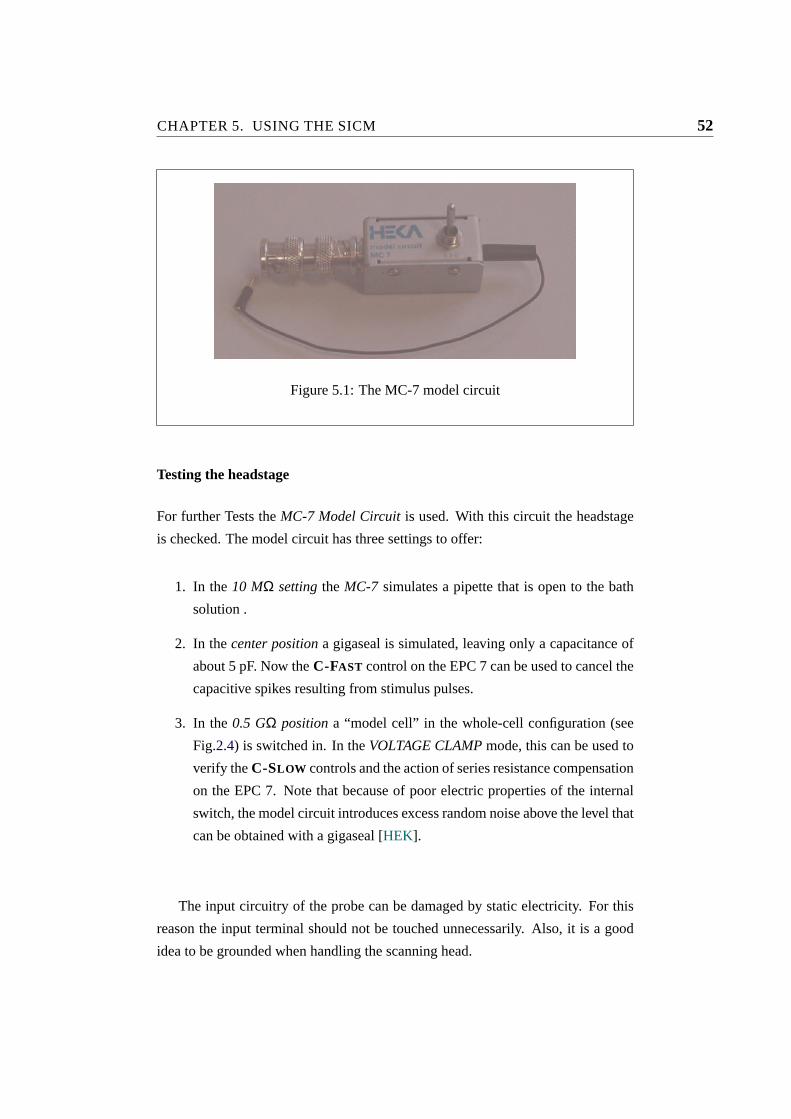
For further Tests theMC-7 Model Circuitis used. With this circuit the headstage

is checked. The model circuit has three settings to offer:

1. In the 10 MΩ settingthe MC-7 simulates a pipette that is open to the bath

solution .

2. In thecenter positiona gigaseal is simulated, leaving only a capacitance of

about 5 pF. Now theC-FAST control on the EPC 7 can be used to cancel the

capacitive spikes resulting from stimulus pulses.

3. In the 0.5 GΩ positiona “model cell” in the whole-cell configuration (see

Fig.2.4) is switched in. In theVOLTAGE CLAMPmode, this can be used to

verify theC-SLOW controls and the action of series resistance compensation

on the EPC 7. Note that because of poor electric properties of the internal

switch, the model circuit introduces excess random noise above the level that

can be obtained with a gigaseal [HEK].

The input circuitry of the probe can be damaged by static electricity. For this

reason the input terminal should not be touched unnecessarily. Also, it is a good

idea to be grounded when handling the scanning head.


We use the model circuit to check the functionality of the headstage.

• Mount theMC-7 to the BNC-connector of the headstage.

• Connect the plug of the MC-7 to theGND connector on top of the headstage.

• Connect the function generator toSTIM. INPUT on the EPC 7.

• Connect theCURRENT MONITOR output of the EPC 7 to the oscillo-

scope.

• Set theMC-7 to 10 MΩ.

• SetM ODE switch toSEARCH.

• SetGAIN selector to10 mV/pA.

• SetSTIM . SCALING EPC to.01.

When applying a square signal from the function generator toSTIM. INPUT

the signal should be reproduced on the oscilloscope. By switching theMC-7 to the

other modes you can watch the behavior of a gigaseal or a whole-cell configuration.

If only drifting noise is measured the isolation between the headstage and the

piezo actuator should be checked before sending the EPC 7 to maintenance. This

has been the most common error in the course of the project.


5.1.5 Testing the EDA unit

To check the functionality of the piezo actuator and its control unit (EDA) we use

theDEMOEDAsoftware provided by the manufacturer.

When switching the EDA unit on or off always take care that theOPEN/CLOSED

LOOP selector is set toopenfor all channels. Be sure that the EDA-unit is turned

on and set all channels to closed loop mode.

• Invoke theDEMOEDAprogram by clicking its icon.

• When the connection is established. The program should show"RS232

aktiv" in the upper left corner.

• Click the TabStandardfunktion .

• Enter an amplitude (Amplitude ) of 70µm for each channel.

• Enter a frequency (Frequenz ) of 50 Hz for each channel.

• Write the data to the EDA by clickingalles schreiben .

• Test each channel by clickingstart . Now you should hear a humming

noise – this is the sound of the vibrating piezo. Stop the channel (stop ) and

proceed with the next one.

The DEMOEDAprogram is also used to configure the EDA-device. See manual

for details [Pie].

5.1.6 Preparing the microscope

The following procedures are necessary to begin any measurement with the SICM.

The thin plastic tube needed to fill the pipette is produced by heating a plastic

needle protection cap over a very small flame. If the flame is too big it will burn the

plastic instead of softening it. When the plastic seems uniformly soft pull it slowly

apart. Cut the produced hollow plastic fiber at the thinnest part.


Filling the pipette

• To fill the pipette with solution dip the pipette tip in filtered solution for some

seconds (tip filling).

• Insert the thin plastic tube of the filling syringe in the back of the pipette and

fill it to a length of 1 cm. There should be no loose drops of solution in the

rest of the pipette (back filling).

• Knock on the side of the pipette with your finger repeatedly to get rid of

small air bubbles.

Mounting and positioning of the pipette

• Put the pipette in the pipette holder in a way that the electrode runs up to the

pipette tip.

• Now place the petri dish containing the sample on the stage of the optical

microscope and plug the pipette holder to the headstage.

• Twist the pipette down until it nearly touches the surface of the solution but

is still slightly tilted. The tilt should be enough to let light pass to the very

tip of the pipette. The headstage EPCHS should be in a high position when

you do this.

• The last step is to mount the bath electrode. Connect it to the small jack on

top of the headstage EPCHS and let the chlorinated silver wire dip into the

bath solution.

After these steps everything is prepared to start measuring: All components are

tested and the pipette is filled and positioned over the sample, ready to enter the

bath solution. By now the desired sample should be centered in the view-field of

the optical microscope.


5.2 Obtaining data

As a start,Matlab should be invoked on the PC. To move the piezo actuator to a

defined upper position, initialize it by executing the functioniniteda in Matlab.

Now the EDA-controller is activated and the position of the pipette is set.

For initialization of the data-acquisition system call the functioninitdaq .

The next step is to insert the pipette into the bath solution.

• Connect the function generator toSTIM. INPUT on the EPC 7.

• Connect the EPC´sCURRENT MONITOR output to the oscilloscope.

• SetM ODE switch toSEARCH.

• SetGAIN selector to10 mV/pA.

• SetSTIM . SCALING selector to0.01.

• Apply a signal from the signal generator toSTIM: INPUT .

• Now, with the pipette not touching the solution, there should be no signal

visible at the oscilloscope. Now is a good time to calibrate the oscilloscope

by switching its input to GND and adjusting the line to zero.

• Move the pipette down with the micromanipulator until it enters the bath. At

this point some pressure can be applied to the pipette if a tube is attached to

the pipette holder. When the bath solution is dirt-free this is not necessary.

In the moment the pipette enters the bath the signal can be seen on the oscil-

loscope. This indicates that the electrical circuit is closed and the pipette is

not clogged.

• Move the pipette tip further down manually. It should now be immersed in

the solution but still some millimeters away from the sample surface. The

signal on the oscilloscope should be stable and not too noisy. If there is much

noise the Faraday cage should be mounted now.


5.2.1 Measuring the pipette resistance

From knowing the applied voltage and the resulting current the pipette resistance

can be calculated and the opening diameter of the tip can be roughly estimated.

• Calculate the applied voltage by multiplying the voltage from the function

generator (the oscilloscope can be used to measure the voltage) with the

value ofSTIM . SCALING .

• Then measure the current answer (reconnect the oscilloscope toCURRENT

MONITOR if necessary). Multiply the voltage displayed on the oscillo-

scope with the value ofGAIN on the EPC 7. The obtained value is the

current flowing through the pipette.

• To calculate the resistance simply use Ohm´s lawI = UR . The resistance

should be some MΩ.

The correlation between resistance and pipette diameter was developed in chap-

ter2.3.


Figure 5.2: The tip near the sample surface viewed under the microscope

5.2.2 Approaching the sample

• Get the pipette tip manually near the target position with the micromanipu-

lator

• Try to bring the tip into the focus of the optical microscope.

• Now move the focus down to your sample and then a little bit up again.

• Move the pipette down with the micromanipulator until the tip is in focus

again.

• Repeat the last steps until the tip is near the sample surface. This may take

some practice — the result should look similar to Fig.5.2. In the shown case

the tip is approximately 20µm above the cells.

• To test if the surface is in reach of the tip call the programprobe(0.998) .

This will give you the distance to the surface. If the resulting height is zero,

lower the tip (14 turn anti-clockwise) and try again.


5.2.3 Recording an approaching curve

Before we start, the pulse generator should be turned off and detached fromSTIM .

I NPUT. Instead of the pulse signal applied before we will now apply a constant

signal. The advantage of a constant signal is the achievement of a smoother curve

and fewer measuring artifacts.

To apply a constant signal we use the Patch-clamp amplifier itself. Turning

VHOLD on the EPC 7 until the answer on the oscilloscope is slightly less than

5V provides a good signal since the analog-to-digital converters of the NI-DAQ

data acquisition card have a range of 0–5 V.

To record an approaching curve, be sure that the tip is in proximity of the

surface. Then enterapproach(val) . Good values are about 0.98 — too low

values will destroy the tip by crashing it into the surface.

Now the tip is moved towards the surface step by step. In every point the

current is measured ,recorded and compared to the initial saturation current. This

takes much longer than the method that will be used to raster the surface but is

more accurate in absolute terms.

Since this program relies on absolute current values, it is prone to drift and

measuring errors.

It is inevitable to experience some broken tips. When the tip breaks the current

jumps to a significantly higher value. After a tip-crash some shards of the destroyed

tip can usually be identified in the optical microscope.


[ IIsat

]

16 18 20 22 24 26 28

0.7

0.75

0.8

0.85

0.9

0.95

1

1.05

[µm]

Figure 5.3: Approaching curve

5.2.4 Starting a scan

When the tip and the specimen are in position, typemap=scan to start the raster

scan. The obtained data is saved in the matrixmapwhich you can use for further

visualization and analysis. You will have to change the values of the program

according to your needs before you start. The Faraday cage should be attached and

any vibration should be prevented during scan.

When viewing through the microscope the scan begins in the upper left corner

of the scanning area – keep this in mind when positioning the tip. Also, the tip

should start its movement over glass and not directly on the specimen.


5.2.5 Processing and visualizing the data

After a scan the obtained data is stored in Matlab´s workspace.

The recorded data will contain unwanted peaks and other failed single measure-

ment points. To remove them and to generally enhance the quality of the picture

you should apply a median filter. A median filter not only removes unwanted peaks

but also sharpens the edges.

With Matlab´s visualization routines a broad range of views can be computed

without any programming.

The entire workspace or selected matrices can be stored and recalled using the

save andload commands in Matlab.

Some Matlab commands:

map2=medfilt2(map) generates a median filtered version ofmapstored

in map2.

map=dlmread(’filename’) reads numeric data from the ASCII delim-

ited file filename into matrixmap

dlmwrite(’filename’,map,delimiter) writes matrixmap into an

ASCII-format file, usingdelimiter to separate matrix elements. A

comma (,) is the default delimiter. Use ’’ to produce tab-delimited files.

plot(map(xcut,:),y) produces a profile of map at the positionxcut

along the y-axis. To get profiles along the x-axis use the form

plot(map(:,ycut),x) . The lists x and y must match the dimen-

sions ofmap.

showmap(map,x,y) computes a lighted surface view ofmap. The lists x

and y must match the dimensions ofmap. An example: if the dimension

of map is 10×10µm with a step-size of 0.5µm the matching lists are

produced by:x=[0.5,0.5,10] ; andy=[0.5,0.5,10] .


5.3 Performed tests

In the beginning we recorded many approaching curves to get the process under

control. A lot of experimentation went into the preparation of the pipettes and

debugging of the first software versions. The first experiments were performed

blind since there was no inverted microscope available. The setup used is shown

in Fig.5.4. In September 2000 the first successful approaches were presented at

the “WE-Heraeus Course – Nanophysics” at the Techical University in Dresden

[Sch00].

In late summer 2001 I received the invitation to Pisa and continued the project

there. Some problems soon got obvious: the initial approach to scan the surface by

step-controlling the tip via the EDA-controller was much to slow.

Therefore we came up with the idea to use an analog output to modulate the

controlling voltage, simultaneously sampling the current to stop the movement

when detecting the surface. This worked out very well. In addition to the higher

scanning speed tip breaks got significantly infrequent due to the dynamic nature of

the process and the increased sensitivity.

With the working prototype we experimented mainly with red blood cells pre-

pared like described in chapter5.1.6.

The microscope was set up in Vienna again, this time in the described config-

uration. Fine tuning of the software was done and the scanning head was installed

on an easily detachable plate for more versatility.


Figure 5.4: An early version of the SICM


5.3.1 Approaching curves

A SICM scan consists of a sequence of approaching curves carried out at every

raster point. To gain quick evidence of the operativeness of the SICM approaching

the surface is the easiest way. With the shape of the approaching curve at hand

estimation of the tip diameter is also possible.

A typical approach curve is presented in Fig.5.5. This curve was recorded

using DC stimulus by the EPC 7 and the functionprobe utilizing differential

measurement. For comparison Fig.5.6 shows a curve that was recorded with a

pulse signal and the use of the functionapproach . The DC stimulated curve is

considerably smoother.

The tilting of the pipette had no noticeable influence on the curves (this would

still be worth investigating again with smaller and in particular more reproducible

pipettes).


500 550 600 650 700 750 800 850 900 950 1000

0.9

0.95

1

1.05

1.1

[samples]

[I/Is

at]

Figure 5.5: Approaching curve, DC stimulus,probe

45 50 55 60 65 70 75

0.8

0.85

0.9

0.95

1

1.05

1.1

[um]

[I/Is

at]

Figure 5.6: Approaching curve, pulse stimulus,approach


Figure 5.7: A Nomarsky phase-contrast picture of red blood cells

5.3.2 Scans

In Fig.5.8 you can see a scan of several red blood cells (erythrocytes) in an area

of 60× 60µm. For comparison Nomarsky phase-contrast pictures are shown in

Fig.5.7. This scan took about 6.5 h and surprisingly the tip was still operable

thereafter. The step-size was 500 nm and the opening diameter of the used tip was

about 400 nm.

The Nomarsky phase-contrast picture was taken after the SICM scan. The fact

that both pictures show the same configuration of cells indicates that the SICM did

not alter the initial cell distribution.


Figure 5.8: A SICM picture of the same cluster

In the SICM picture the resolution is evidently better than in the phase-contrast

picture. Note that the gaps between the cells are clearly recognizable. As opposed

to phase-contrast microscopy or similar methods the whole three-dimensional to-

pography of the specimen is recorded.

The results from another scan are illustrated in Fig.5.9. Here a single blood

cell is pictured. The area of this scan is 15×15 µm and the resolution is 500 nm

again. The pipette used for this scan was slightly smaller with a estimated diameter

of 300 nm.


Figure 5.9: Scan of a single cell

CHAPTER 6. PROPOSED IMPROVEMENTS 69

Chapter 6

Proposed improvements

Reprogramming the software: The pictures taken are of good quality but the

scanning process takes too much time. To reach a higher scanning speed

it will be necessary to re-write the code in C/C++. Matlab is an interpreted

language and therefore the bottleneck of the measurement system.

The reprogrammed SICM will scan approximately 20–100 times faster than

with the present software. The speed will be improved in two ways: exe-

cution speed is dramatically higher and the driver support for the DAQ-card

will be better (the DAQ-Toolbox in Matlab requires the program to pause for

same tenths of a second after each measurement).

In the course of reprogramming the software a user-friendly graphical user

interface should be designed. The Matlab functions will not be obsolete

when new software exists. They still have their use for experiments and

testing purposes.

A faster computer: The usage of a faster computer will speed up the workflow

considerably — especially when working with Matlab. A faster computer

will also influence the the scanning speed to a small extent. A DAQ-card

with higher sampling frequency will also boost the scanning speed.

Acquisition of a puller: The purchase of a good pipette-puller is required. To

get the pulling process under control a lot of research should be invested.

A bubble test or some similar method has to be developed to estimate the

opening diameter of the produced pipettes. A Laser puller is recommended

CHAPTER 6. PROPOSED IMPROVEMENTS 70

for research requiring high resolutions. For less demanding applications a

good Brown-Flaming type puller will in be sufficient.

Use of the Computer as function generator:An analog output of the NI-DAQ

should be used for generation of the stimulation signal. To get good mea-

surements the voltage should only be turned on while approaching the sur-

face. Additionally the sign of the voltage should be reversed in each scan-

ning point when scanning cells to prevent polarization which could damage

the cells.

Construction of a perfusion chamber: To expose the specimen to modified bath

solutions a perfusion chamber should be constructed. This is especially a

must when trying to investigate ion-channels. Some tips about perfusion

systems and different methods to quickly change the bath solution can be

found in [ND96]. The perfusion process could also be controlled by the

NI-DAQ card.

Experiments:

Calibration The absolute accuracy of the SICM has to be increased by calibrating

it with known micro-structures.

Frequency- and step-responsesin dependence of the distance to the specimen

and the used pipette should be investigated.

Localization of ion channels For this experiment a two pass method can be used.

In the first pass ion channels in the cell surface are chemically blocked. The

SICM scans the surface as usual to get a picture of the topography of the

cell.

In the second pass the ion channels are activated and the SICM follows the

previously scanned surface, thus detecting the ion currents and localizing the

channels.

CHAPTER 7. CONCLUSION 71

Chapter 7

Conclusion

The Project to construct a Scanning Ion Conductance Microscope (SICM) from

scratch was initiated in February 2000 by Dr. Ille Gebeshuber. After collecting

theoretical background information and literature studies appropriate hardware was

selected and ordered. A Finnish exchange student named Perttu Niemela (Univer-

sity of Oulu) assisted me in this task. In September 2000 the first results were

presented at the “WE-Heraeus course Nanophysics” in Dresden [Sch00].

In summer 2001 I was invited to Pisa where most of the actual project was

done. A control solution for the time critical approaching process was found and

a working prototype was assembled and tested. The work in Pisa was done in

cooperation with Prof. Dr. Mario Pellegrini, Prof. Dr. Donatella Petracchi and Prof.

Dr. Cesare Ascoli at theDipartimento di Fisiologia e Biochimica.

After being timed out for the duration of my military service the microscope

has been re-installed and further enhanced at theInstitute of Chemical Engineering

(Technical University of Vienna)with the help of Prof. Dr. Helmut Stachelberger.

The SICM is operative and its usefulness has been shown. Pictures of red blood

cells have been taken as proof of concept. The constructed SICM will be utilized

in research projects at the Institute of Chemical Engineering by Prof. Dr. Helmut

Stachelberger.

LIST OF ABBREVIATIONS 73

List of abbreviations

AFM . . . . . . . . . . . . . . . . . . . . . . . . . . . . . . . . . Atomic force microscope

AMFM . . . . . . . . . . . . . . . . . . . . . . . Attractive mode force microscope

DIC . . . . . . . . . . . . . . . . . . . . . . . . . . . . . . . . . Differential phase contrast

EFM . . . . . . . . . . . . . . . . . . . . . . . . . . . . Electrostatic force microscope

FFM . . . . . . . . . . . . . . . . . . . . . . . . . . . . . . . . . Friction force microscope

MFM . . . . . . . . . . . . . . . . . . . . . . . . . . . . . . . Magnetic force microscope

NI-DAQ . . . . . . . . . . . . . . . National instruments data acquisition card

SAM . . . . . . . . . . . . . . . . . . . . . . . . . . . . . Scanning acoustic microscope

SHFM . . . . . . . . . . . . . . . . . . . . . . . . . . . . . . . . . Shear force microscope

SICM . . . . . . . . . . . . . . . . . . . . Scanning ion conductance microscope

SNOM . . . . . . . . . . . . . . . . . . . Scanning near-field optical microscope

SPM . . . . . . . . . . . . . . . . . . . . . . . . . . . . . . . Scanning probe microscope

STM . . . . . . . . . . . . . . . . . . . . . . . . . . . Scanning tunnelling microscope

SThM . . . . . . . . . . . . . . . . . . . . . . . . . . . . Scanning thermal microscope

UHV . . . . . . . . . . . . . . . . . . . . . . . . . . . . . . . . . . . . . . . Ultra high vacuum

LIST OF FIGURES 74

List of Figures

1.1 A scan of red blood cells with applied median filter. . . . . . . . 11

2.1 Principle of a STM . . . . . . . . . . . . . . . . . . . . . . . . . 15

2.2 Principle of a AFM . . . . . . . . . . . . . . . . . . . . . . . . . 17

2.3 Patch-clamp. . . . . . . . . . . . . . . . . . . . . . . . . . . . . 21

2.4 Cell configurations. . . . . . . . . . . . . . . . . . . . . . . . . 22

2.5 Principle of a SICM. . . . . . . . . . . . . . . . . . . . . . . . . 24

2.6 Model of a micro-pipette tip . . . . . . . . . . . . . . . . . . . . 27

2.7 Calculated and measured approaching curves. . . . . . . . . . . 29

3.1 The Scanning Head of the SICM. . . . . . . . . . . . . . . . . . 31

3.2 The Instrument Rack. . . . . . . . . . . . . . . . . . . . . . . . 32

3.3 The pipette holder and a pipette. . . . . . . . . . . . . . . . . . . 36

3.4 Scanning electron microscope image of a micropipette. . . . . . 38

3.5 Narishige Pipette puller. . . . . . . . . . . . . . . . . . . . . . . 41

4.1 Diagram of the signal paths of the SICM. . . . . . . . . . . . . . 46

5.1 The MC-7 model circuit . . . . . . . . . . . . . . . . . . . . . . 52

5.2 The tip near the sample surface viewed under the microscope. . . 58

5.3 Approaching curve. . . . . . . . . . . . . . . . . . . . . . . . . 60

LIST OF FIGURES 75

5.4 An early version of the SICM. . . . . . . . . . . . . . . . . . . . 63

5.5 Approaching curve, DC stimulus,probe . . . . . . . . . . . . . 65

5.6 Approaching curve, pulse stimulus,approach . . . . . . . . . . 65

5.7 A Nomarsky phase-contrast picture of red blood cells. . . . . . . 66

5.8 A SICM picture of the same cluster. . . . . . . . . . . . . . . . 67

5.9 Scan of a single cell. . . . . . . . . . . . . . . . . . . . . . . . . 68

BIBLIOGRAPHY 76

Bibliography

[Aea88] Alexander and Schneir et al. An atomic resolution afm implemented

using an optical lever.Journal of Applied Physics, 65:164–167, 1988.

[AP03] Alexeev and Popkov. Magnetic Force Microscopy. NT-

MDT, State Institute for Physical Problems, Moscow, 2003.

http://www.ntmdt.ru/applicationnotes/MFM/.

[Bea82] Binnig and Rohrer et al. Surface studies by scanning tunneling mi-

croscopy.Physical Review Letters, 49:57–61, 1982.

[BQG86] Binnig, Quate, and Gerber. Atomic force microscopy.Phys. Rev. Lett.,

56:930–933, 1986.

[BR87] Binnig and Rohrer. Scanning tunneling microscopy – from birth to

adolescence.Rev. Mod. Phys., 59:615–625, 1987.

[CGL92] A. Cavalie, R. Grantyn, and H. D. Lux.Practical Electrophysiological

Method, chapter Fabrication of patch clamp pipettes, pages 235–241.

Wiley-Liss, New York, 1992.

[Dea89] Drake and Prater et al. Imaging crystals, polymers, and processes in wa-

ter with the atomic force microscope.Science, 243:1586–1589, March

1989.

[GMS94] Goosens, Mittelbach, and Samarin.The LATEX Companion. Addison-

Wesley, 2 edition, 1994.

[Hea89] Hansma and Drake et al. The scanning ion-conductance microscope.

Science, 24:641–643, February 1989.

BIBLIOGRAPHY 77

[HEK] HEKA elektronik GmbH, Wiesenstraße 71, 67466 Lambrecht, Ger-

many.EPC8/EPC7 Manual. in german language.

[Kam95] Jorg Kamp. Aufbau und Erprobung eines kombinierten

Rasterionenleitungs- und Scherkraftmikroskops. Diploma thesis,

Physikalisches Institut der Westfalischen Wilhelms-Universitat, March

1995. in german language.

[KBM97] Korchev, Bashford, and Milovanovic. Scanning ion conductance mi-

croscopy of living cells. Biophysical Journal, 73:653–658, August

1997.

[Kea00] Korchev and Negulyaev et al. Functional localization of single active

ion channels on the surface of a living cell.Nature Cell Biology, pages

616–619, September 2000.

[KMB97] Korchev, Milovanovic, and Bashford. Specialized ion-conductance mi-

croscope for imaging of living cells.Journal of Microscopy, 188(1):17–

23, October 1997.

[Kop96] Helmut Kopka.LATEX-Einfuhrung (Band 1). Addison-Wesley, 2 edition,

1996.

[Lam94] Leslie Lamport. LATEX – A Document Preparation System. Addison-

Wesley, 2 edition, 1994.

[MDH87] Marti, Drake, and Hansma. Atomic force microscopy of liquid-covered

surfaces: Atomic resolution images.Appl. phys. Lett., 51:484–486,

1987.

[Mea88] Marti and Elings et al. Scanning probe microscopy of biological sam-

ples and other surfaces.Journal of Microscopy, 152:803–809, 1988.

[ND96] Numberger and Draguhn.Patch-Clamp Technik. Spektrum Akademis-

cher Verlag, 1996.

[NS92] Neher and Sakmann. Die Erforschung von Zellsignalen mit der Patch-

Clamp-Technik.Spektrum der Wissenschaft, pages 48–56, May 1992.

in german language.

BIBLIOGRAPHY 78

[OR95] O´Reilly and Richardson. A practical vibration isolation workstation

for electrophysiology.journal of Neuroscientific Methods, 60:175–180,

1995.

[PH91] Prater and Hansma. Improved scanning ion-conductance micro-

scope using microfabricated probes.Review of Scientific Instruments.,

62(11):2634–2637, November 1991.

[Pie] Piezosystem jena GmbH, Prussingstr. 27 D-07745 Jena/Thuringen.Be-

dienungsanleitung EDA2/3. in german language.

[PLH96] Proksch, Lal, and Hansma. Imaging the internal and external pore struc-

ture of membranes in fluid: Tappingmode scanning ion conductance

microscopy.Biophysical Journal, 71:2155–2157, October 1996.

[Sch90] E. Schwab. Aufbau und Erprobung eines kombinierten Rasterionen-

leitungsmikroskops (RILM). Diploma thesis, Wiesbaden, 1990. in ger-

man language.

[Sch00] Stefan Schraml. Setup of a SICM. WE-Heraeus Ferienkurs

Nanophysik, Sept. 2000. poster presentation.

[Ste95] Neil Stephenson.The Diamond Age. Penguin Book Ltd., 1995.

[WW86] Williams and Wickramasinghe. Scanning thermal profiler.Appl. Phys.

Lett., 49:1587–1589, 1986.

SETUP AND APPLICATION OF A

Documents

Transcript of SETUP AND APPLICATION OF A