Journal of the Faculty of Environmental Science and Technology. Okayama UniversityVol.1. No.1. pp.193-198. March 1996

Settlement Prediction Method Using Observed Settlement li?locity

Kiyoshi SHIMADA*, Sin-ichi NISHIMURA* and Hiroaki FUJII*

(Received January 16 . 1996)

Abstract This paper presents a new method for prediction of consolidation

settlements bf soft grounds. The method is based on the theoretical result which shows

that the settlement velocity of soft grounds non-improved or improved with sand drains

decreases exponentially with time. Final settlements can be easily derived from the

regression analysis for the relationship between the elapsed time and the observed

settlement velocity. The method has advantages of its simplicity and capability to give

the satisfactorily good estimate of the consolidation settlements, and also the support of

the theoretical background.

Key Words: consolidation, settlement prediction, soft ground, sand drains, one­

dimensional consolidation

1. INTRODUCTIONWe sometimes fail to obtain the acceptable

estimate of consolidation settlements of soft

grounds even though adopting an elaborate

constitutive equation in finite element method.

The failure is probably due to uncertainty of

soil constants and boundary conditions, etc.

Accordingly, several methods to predict settle­

ments using observed data have been proposed

and widely used. (Yoshikuni et al. 1981)

This paper presents a new method of settle­

ment prediction using observed settlement

velocity. The method is based on the theoretical

result which shows that the settlement velocity

of soft grounds non-improved or improved

with sand drains decreases exponentially with

time. The final settlement can be easily derived

from the regression analysis for the relationship

between the elapsed time and the observed

settlement velocity.

2. RELATIONSHIP BETWEEN TIMEAND SETTLEMENT VELOCITY IN

SOFT GROUND IMPROVED WITHSAND DRAINS

The approximate solution of Barron's

consolidation equation for a sand drain (Barron

1948, Richart 1957, and Yoshikuni 1979) is as

follows:

S(t)=Sj{ 1 - exp[at]} (1)

where t is the time measured from the start of

consolidation, Set) the settlement at the time t,

* Department of Environmental Management Engineering

193

1941. Fac. Environ. Sci. and Tech., Okayama Univ. 1 (1) 1996

Sf the final settlement, and

-8 Cha=-- --

F(n) d 2'

e

where ao =InAo and al =AI-

Since settlement observations are usually

made in a certain interval, we cannot obtain the

derivative ( dS Idt) like a mathematical deriva­

tive of a continuous function. Then we define

the observed settlement velocity (tiS I I1t)

(9)

(8)

(7)

(6)

and also the settlement curve from Eq.(l).

The settlement velocity during embankment

should not be used in the analysis because

Eq.(l) can be held only with such an assump­

tion that all loads are applied simultaneously.

Hence it is necessary to introduce a new coordi­

nate system (t', S') whose origin is located at

(t= to, S= So) on the settlement curve Eq.(l).

We then obtain the following equation.

S'(t')=Si{ 1 - exp[at']}

where S(t) = So + S'(t') and Sf= So+ Sf.

Applying the same procedure to the relation­

ship between the elapsed time (t') and the

observed settlement velocity (11.5'll1t') , we

can obtain the final settlement Sf from the

regression parameters A '0, A'1 on Eq.(7) as

A'S' 0f=-Y'

1

Applying the model to the relationship between

the elapsed time (t) and the observed settle­

ment velocity (I1S1I1t), we can find the regres­

sion parameters a0, a1. Then we can calculate

Ao, Al and the final settlement Sf from Eq.(4)

as

instead of (dS Idt). Fig. 1 shows the calcula­

tion procedure of the observed settlement

velocity. When we obtain observed data at

Point A and B whose time and settlement are

(ta, Sa)' (tb, Sb) respectively, we define the

observed settlement velocity at time t c with the

next equations:

S -SAS / At = b a

tb - ta

(5)

Time, I

--c:CI)

ECI)

i(J)

Eq.(2) can be rewritten as follows:

y =Ao exp[ Al x] (3)

where y = dSldt, x = t, and

Ao=- aSf , Al = a (4)

Transforming the variables as Y = In (y) and X

=x, we obtain the following linear regression

model.

n 2 3n 2 -1 deF(n)= 2 In(n) - 4n2 ' n=-d

n -1 w

where Ch is the coefficient of consolidation, de

is the equivalent effective diameter of a sand

drain, and d w the diameter of a sand drain.

The differentiation of Eq.( 1) with respect to

time (t) gives the settlement velocity (dSldt),

dSdt = - aSf exp[ at] . (2)

Fig. 1 Calculation of observed settlement

velocity (ASIAI)and also the total settlement S as

K. SHIMADA et al. / Settlement Prediction Method Using Observed Settlement Velocity195

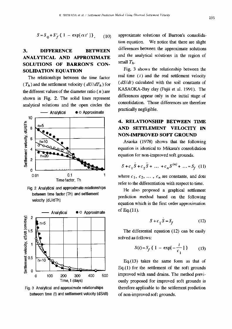
S=So+S.r{ 1 - exp[at' n. (10)

3. DIFFERENCE BETWEEN

ANALYTICAL AND APPROXIMATE

SOLUTIONS OF BARRON'S CON­SOLIDATION EQUATION

The relationships between the time factor

(Th) and the settlement velocity ( dUldTh) for

the different values of the diameter ratio (n ) are

shown in Fig. 2. The solid lines represent

analytical solutions and the open circles the

- Analytical • 0 Approximate

approximate solutions of Barron's consolida­

tion equation. We notice that there are slight

differences between the approximate solutions

and the analytical solutions in the region of

small Th.

Fig. 3 shows the relationship between the

real time (t) and the real settlement velocity

( dSIdt) calculated with the soil constants of

KASAOKA-Bay clay (Fujii et al. 1991). The

differences appear only in the initial stage of

consolidation. Those differences are therefore

practically negligible.

where Ct, cz• ...• en are constants, and dots

refer to the differentiation with respect to time.

He also proposed a graphical settlement

prediction method based on the following

equation which is the first order approximation

of Eq.(l1).

4. RELATIONSHIP BETWEEN TIME

AND SETTLEMENT VELOCITY IN

NON-IMPROVED SOFT GROUND

Asaoka (1978) shows that the following

equation is identical to Mikasa's consolidation

equation for non-improved soft grounds.

... (n)S+c1S+cZS+ ... +cnS + ",=Sf (11)

• 0 Approximate- Analytical

.r:.I-::!:2 8:>'0

>.13 60

~4-l::

CI)

ECI) 2ECI)

C/)

00.01 0.1 1

Time factor, Th

Fig. 2 Analytical and approximate relationshipsbetween time factor (Th) and settlement

velocity (dU/dTh)

10 ....------...--------,

(12)

Eq.(13) takes the same form as that of

Eq.(1) for the settlement of the soft grounds

improved with sand drains. The method previ­

ously proposed for improved soft grounds is

therefore applicable to the settlement prediction

of non-improved soft grounds.

tSet) =Sf { 1 - exp[ - -] } (13)

c1

The differential equation (12) can be easily

solved as follows:

500400100 200 300Time, t (days)

Fig. 3 Analytical and approximate relationshipsbetween time (t) and settlement velocity (dS/dt)

>: 2 w------.---...,......--.------r-----,as

::!:2

5';: 1.5 1-\----+----+--+---+---1::!:2C/)'0

~1o~1i 0.5ECI)

~ 0 L_--l._~~~;;;;;;;;t;g;=d..o()o-J

o

196J. Fac. Environ. Sci. and Tech.. Okayama Univ. I (1) 1996

o

- t'=O to t'=60 days- t'=O to t'=114 days- all data

100 200 300 400 500Time, r (days)

Fig. 5 Relationship between time (t') and settlementvelocity (dS'/dt') of Point H in field NO.7

....~ 1en"'C

~(,)o~ 0.5'EQ)

EQ) 0~ 0 L_..L_--.l_-=~~~~~en

o

-o Observed == Regression line

KASAOKA-Bay reclaimed land, OKAYAMA.

The ground had been improved with packed

sand drains and preloading embankments (Fujii

et al. 1991, Shimada et al. 1992).

Figs. 4 and 5 show the relationships

between time (t') and the settlement velocity (

/i,S'/!i.t') for Point H in the field No.4 and

No.7, respectively. The time of the completion

of embankment is adopted as the origin of (t',

S') coordinate system. The open circles show

the observed settlement velocities, The exponen­

tially decaying lines are the result of the regres­

sion analysis with the least square method. The

- 1'=0 to t'=91 days- t'=Oto t'=190 days- all data

100 200 300 400 500Time, r (days)

Fig. 4 Relationship between time (t') and settlement

velocity (dS'/dt') of Point H in field No.4

-l::Q)

EQ)

~ 0 L...-_--'-__...L--_----L.....u.~~_ __'

eno

~1.5~E~....~en"'C

~'0o~ 0.5 I--~~--+--_+---+--_____j

5. PREDICTED SETTLEMENTS OFSOFf GROUNDS IMPROVED WITHPACKED SAND DRAINS

The proposed method is applied to the

settlement prediction of the soft grounds in

o Observed - Regression line

Atkinson and Bransby (1978) obtained an

approximate solution of Terzaghi's consolida­

tion equation for non-improved soft grounds.

They approximate the isochrones with parabo­

las. The solution has the same form as that of

Eq.(13), and accordingly the settlement veloci­

ty decreases exponentially with time.

t'=O

200all data

o Observed- Predicted

Time (days)o 100 200 300 400 500 600

O~-....----.----r-----r----r----,

200

_ 50E~-l::Q) 100EQ)

~en 150

all data

o Observed- Predicted

_ 50 I--~~-+---+---+--_+-_____j

E~

'E~ 100Q)

EQ)

en 150

Time (days)o 100 200 300 400 500 600

O~.---.,....--...,.---,--....,...----r-----,

Fig. 6 Settlement prediction for Point H in field NO.4 Fig. 7 Settlement prediction for Point H in field NO.7

K. SHIMADA et al. / Settlement Prediction Method Using Observed Settlement Velocity197

thin solid lines are derived from all observed

data. The thick solid lines are derived from the

data observed from t' =0 to t' =91 days, 190

days in Fig. 4, and t'=O to t'=60 days, 114

days in Fig. 5, respectively.

Fig. 6 shows the results of the settlement

prediction for Point H in the field No.4. The

open circles represent observed settlements.

Three solid lines are settlement curves predicted

at t'=91 days, 190 days and predicted with all

observed data, respectively. The prediction is

also applied to the Point H in the field No.7

and results are shown in Fig. 7. Three settle­

ment curves are predicted at t' = 60 days, 144

days and predicted with all observed data,

respectively.

These figures show that the observed settle­

ments can be expressed successfully when all

observed data are used, i.e., the settlement of

soft grounds improved with sand drains can be

calculated with Eq.(1). It is also clear from the

figures that the prediction accuracy becomes

improved more with the longer elapsed time

from the completion of embankment.

The prediction accuracy is presented in Fig.

8 as the relationship between V' and Rs . These

parameters are defined with the following

equations by Yoshikuni et a1. (1981).

V' = Observed settlement at the time of predictionLast observed settlement

R = Predicted settlement for the time of last observation

s Last observed settlement

(14)

where V' refers to the equivalent degree of

consolidation at the time of prediction. Rs

shows the accuracy of prediction. When there

is no error in prediction, Rs becomes unity.

Yoshikuni et a1. (1981) compared the

accuracies of several prediction methods with

their observed data. Their results are summa­

rized in Table 1 which shows V' at some levels

of Rs• The smaller value of V' at the same level

of Rs indicates good prediction.

The result of the proposed method with the

data of KASAOKA-Bay reclaimed land is also

presented in the table. The method gives the

satisfactorily good estimate of settlements.

Table 1 Prediction methods and their accuracies(From Yoshikuni et al.(1981))

Fig. 8 Predicting accuracy in Kasaoka-bay

reclaimed land

_ 4H ~ 6C --[]- 7H

~ 5E --+- 7G1

cr.'" 0.9o~ 0.8'E~ 0.7Q)

~ 0.6

0.50.2 0.4 0.6

U'0.8

R s R s=O.7 R s=O.8 R s=O.9 R s=O.95Methods

Hyperbolic U'=O.4 U'=O.6 U'=O.7 U'=O.8Monden U'=O.6 U'=O.7 U'=O.8 U'=O.9Hoshino U'=O.4 U'=O.5 U'=O.6 U'=O.7Asaoka U'=O.5 U'=O.65 U'=O.8 U'=O.9

Proposed I U'=O.5 I U'=O.55 I U'=O.7 I U'=O.8

6. PREDICTED SETTLEMENTS OFNON-IMPROVED SOFf GROUND

Fig. 9 shows the relationships between time

(t') and the settlement velocity (/lS'/!i.t') for a

non-improved soft ground. The observed data

1981. Fac. Environ. Sci. and Tech.. Okayama Univ. 1 0) 1996

Fig. 9 Relationship between time (t') and settlementvelocity (dS'/dt') of non-improved soft ground

ReferencesAboshi, T. (1969) : Soil Mechanics (Edited by T.

Mogami), Gihodo-shuppan, Tokyo, 464-465 (inJapanese).

Asaoka, A. (1978) : Observational procedure ofsettlement prediction, Soils and Foundations, 18(4),87-101.

Atkinson, J.H. and Bransby, P.L. (1978) : Themechanics of soils, McGraw-Hill, London.

Barron, R.A. (1948) : Consolidation of fine-grainedsoils by drain wells, Trans of ASCE, 113, 718-754.

Fujii, H., Shimada, K., Nishimura, S. and Tajiri, N.(1991) : Determination of soil parameters with

standard consolidation tests and its application toftnite element analysis, Trans. of JSIDRE, 154, 1­16 (in Japanese).

Richart, F.E.Jr. (1957) : A review of the theories forsand drains, Proc. of ASCE, 83(SM3), 1301-1 ­1301-38.

Shimada, K., Fujii, H., Nishimura, S. and Tajiri, N.(1992) : Plane strain ftnite element analysis forconsolidation settlement in soft ground improvedwith packed sand drains, Trans. of JSIDRE, 162, 1-7(in Japanese).

Yoshikuni, H., Inoue, T., Sumioka, N., Hara, H.(1981) : On the characteristics of settlementprediction methods by monitoring, Tsuchi-to-kiso,29(8),7-13 (in Japanese).

Yoshikuni, H. (1979) : Design and perfonnancemanagement for vertical drains, Gihodo-shuppan,Tokyo (in Japanese).

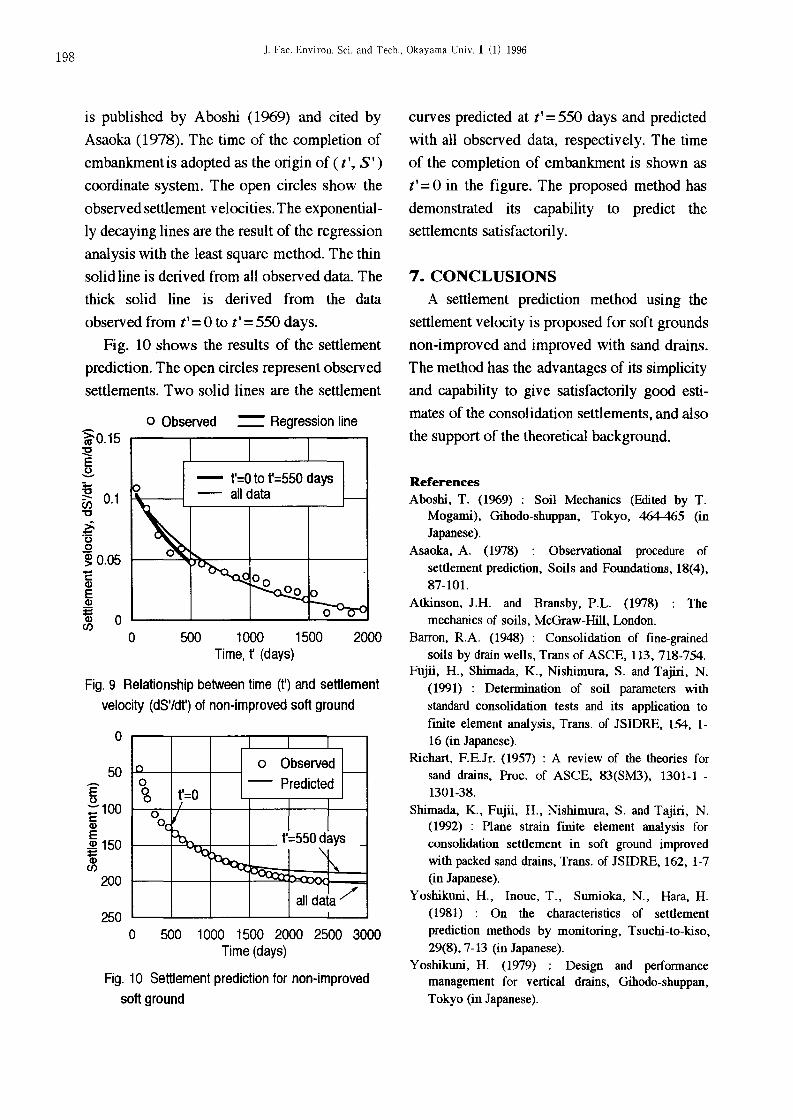
curves predicted at t' = 550 days and predicted

with all observed data, respectively. The time

of the completion of embankment is shown as

t' =0 in the figure. The proposed method has

demonstrated its capability to predict the

settlements satisfactorily.

7. CONCLUSIONS

A settlement prediction method using the

settlement velocity is proposed for soft grounds

non-improved and improved with sand drains.

The method has the advantages of its simplicity

and capability to give satisfactorily good esti­

mates of the consolidation settlements, and also

the support of the theoretical background.

2000

- t'=O to t'=550 days- all data

500 1000 1500Time, f (days)

o Observed ~ Regression line

I I

n 0 Observed -0 - Predicted<t> t'=O

I I0 'I

tL550dlys°c Po.. -

"Q~

\\..

all data/'

oo

Eo::;-100c:(I)

E~ 150i(J)

200

250o 500 1000 1500 2000 2500 3000

Time (days)

Fig. 10 Settlement prediction for non-improvedsoft ground

o

50

is published by Aboshi (1969) and cited by

Asaoka (1978). The time of the completion of

embankment is adopted as the origin of ( t', S')

coordinate system. The open circles show the

observed settlement velocities. The exponential­

ly decaying lines are the result of the regression

analysis with the least square method. The thin

solid line is derived from all observed data. The

thick solid line is derived from the data

observed from t'=O to t'=550 days.

Fig. 10 shows the results of the settlement

prediction. The open circles represent observed

settlements. Two solid lines are the settlement

~0.15:l:2E~

~(J) 0.1"t:l

;i-'0o~0.05EQ)

EQ)

~(J)