j /) r"

/o/ .....LINEAR AND ORDER STATISTICS COMBINERS FOR PATTERN

CLASSIFICATION

Kagan Tumer

NASA Ames Research Center

MS 269-4, Moffett Field, CA, 94035-I000,Q

kaganOptolemy.arc, nasa.gov

Joydeep Ghosh

Department of Electrical and Conlputer Engineering,

University of Texas, Austin, TX 78712-1084

ghosh Opine. ece. u t exas. edu

Abstract

Several researchers have experimentally shown that substantial improvements can be ob-

tained in difficultpattern recognition problems by combining or integratingthe outputs of mul-

tipleclassifiers.This chapter provides an analyticalframework to quantify the improvements in

classificationresultsdue to combining. The r_sultsapply to both linear combiners and order

statisticscombiners. We firstshow that to a firstorder approximation, the error rate obtained

ovor and above the Bayes error rate, L_"7_'g_v pioportTonaI l_0-_Ile variance dF_he aclmar_Ie(us'.on

boundaries around the Bayes optimum boundary. Combining classifiers in output space reduces

this variance, and hence reduces the "added" error. If N unbiased classifiers are combined by

simple averaging, the added error rate can be reduced by a factor of N if the individual errors in

approximating the decision boundaries axe uncorrelated. Expressions are then derived for linear

combin,_rs which are biased or correlated, and the effect of output correlations on ensemble per-

formance is quantified. For order statistics based non-linear combiners, we derive expressions

that indicate how much the median, the maximum and in general the ith order statistic can

improve classifier performance. The analysis presented here facilitates the understanding of

the relationships among error rates, classifier boundary distributions, and combining in output

space. Experimental results on several public domain data sets axe provided to illustrate the

benefits of combining and to support the analytical results.

1 Introduction

Training a parametric classifier involves the use of a training set of data with known labeling to

estimate or "learn" the parameters of the chosen model. A test set, consisting of patterns not

previously seen by the classifier, is then used to determine the classification performance. This

ability to meaningfully respond to novel patterns, or generalize, is an important aspect of a classifier

system and in essence, the true gauge of performance [38, 77]. Given infinite training data, consistent

classifiers approximate the Bayesian decision boundaries to arbitrary precision, therefore providing

similar generalizations [24]. However, often only a limited portion of the pattern space is available or

observable [16, 221 Given a finite and noisy data set. different cla._sifiers typically provide different

generalizations by realizing different decision boundaries [26!. For example, when classification is

performe(l using ;t multilayere(l, feed-forward artificial neural network, different weight, initializations,

https://ntrs.nasa.gov/search.jsp?R=20020024756 2019-01-12T13:04:09+00:00Z

Combiner I

"'-....f md ...

l o.... ",...."" ,,

u'"i [

i • • • [ ClassifierClassifier 1 m

I [

....o..°.°°

Set 1 Set 2

--.°..

"'-.° . .

"--.....

• • • lassifier

o°...°-

Raw Dhta from Observed Phenomenon ]

"'"'I

Feature• • [ Set M

o1_ v°

.°°".°

oO.°°

°°°,..

-Fig(i_-l-) Comb_g g/)"-(_:g;3:7-Tt_U_d lines leading to fma repre._ent tile &Tcision of a specific

classifier, while the dashed lines lead to f_o,,,n the output of the combiner.

• relates the location of the decision boundary to the classifier error.

The rest of this article is organized as follows. Section 2 introduces the overall framework for

estimating error rates and the effects of combining. In Section 3 we analyze linear combiners,

and derive expressions for the error rates for both biased and unbiased classifiers. In Section 4,

we examine order statistics combiners, and analyze the resulting classifier boundaries and error

regions. In Section 5 we study linear combiners that make correlated errors, derive their error

reduction rates, and discuss how to use this information to build better combiners. In Section 6. we

present experimental results based on real world problems, and we conclude with a discussion of the

implications of the work presented in this article.

2 Class Boundary Analysis and Error Regions

Consider a single classifier whose outputs are expected to approximate the corresponding a posteriori

class probabilities if it is reasonably well trained. The decision boundaries obtained by such a

classifier are thus expected to be close to Bayesian decision boundaries. Moreover, these boundaries

will tend to occur in regions where the number of training samples belonging to the two most locally

dominant ck_ses (say. classes i and j) are comparable.

We will focus our analysis on network performance _ound the decision boundaries. Consider the

boun,lary between cla.sses i anti j for a single-dime,lsion_fl input (the extension to multi-dimensional

inputs is discussed m [73]). First, let us express the output response of the ith unit of a one-of-L

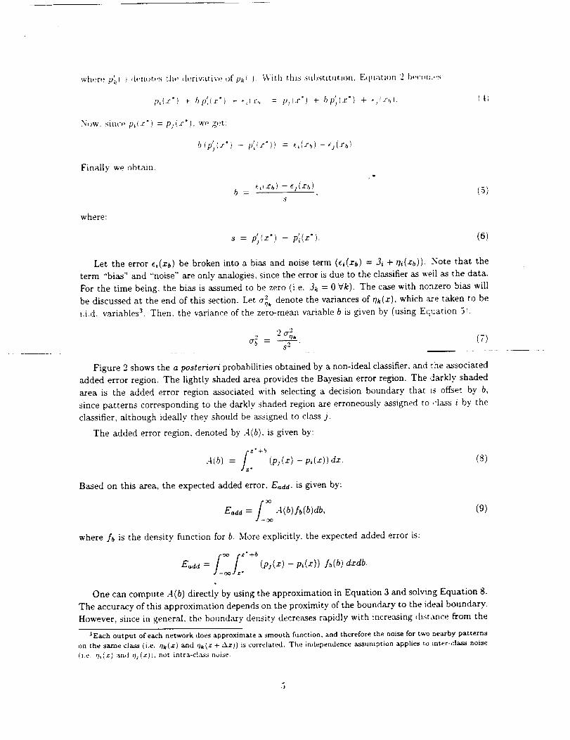
wher_ p' __: ) [enot-s _;he ,[ertv:tt.ive of Pk! I _5/ith tllt:_ subsr.Ltutiou, Equation ') I'J,_,:on.,.._:

l),(.c') 4- bp',I_:'i _- **I;:,,_ = p;i.v'l + bp'l(.g') + ,j:;';,)

Now. since p_ z') = pj(_"), we g_t,:

b (p'2(z') - p',!;'i! = <(r_) - %(.r_t

Finally we obtain:

b (5)

where:

s p'j(x" - '(x'"= p,, ). (6)

Let the error e,(xb) be broken into a bias and noise term (ei(xb) = 3_ + rh(xb)). Note that the

term "'bias" and "'noise" are only analogies, since the error is due to the classifier as well as the data.

For the time being, the bias is assumed to be zero (i.e. 3k = 0 gk). The case with nonzero bias will

be discussed at the end of this section. Let a_ denote the variances of r/k(x), which are taken to be

i.i.d, variables a. Then. the variance of the zero-mean variable b is given by (using Equation 5):

"2

'2%, (7)

Figure 2 shows the a posteriori probabilities obtained by a non-ideal classifier, and ,'he associated

added error region. The lightly shaded area provides the Bayesian error region. The darkly shaded

area is the added error region associated with selecting a decision boundary that is offset by b,

since patterns corresponding to the darkly shaded region are erroneously assigned to ,:lass i by the

classifier, although ideally they should be assigned to class 2.

The added error region, denoted by A(b). is given by:

t* X'_-b

= / (p2(x) - pi(x)) dx. (8),I z

Based on this area, the expected added error. EaUd, is given by:

/5E_dd = A(b)fb(b)db, (9)

where fb is the density function for b. More explicitly, the expected added error is:

,_ f:" +bf

E(,,tct = ] j:: (pj(x) - p,(x)) fb(b) dxdb.J- O0 *

One can compute A(b) directly by using the approximation in Equation 3 and solving Equation 8.

The accuracy of this approximation depends on the proximity of the boundary to the ideal boundary.

However, since in general, the bound_y density decreases rapidly with increasing distance from the

JEach output of each network does approximate a smooth function, and therefore the noise for two nearby pattern_

on the sazne cia_:_ (i.e. Ok(.r) and r_a(x + _-x)) is correlated. The imlependence a..mumption applies to inter-class noise

(i.e. rh(._) and _b(x)}, not intra-cla.ss noise.

3 Linear Combining

3.1 Linear Combining of Unbiased Classifiers

Let us now ,iivert our attention to tile effects of linearly combining multiple classifiers. [n what

follows, the combiner denoted by ave performs an arithmetic average m output space. If N classifiers

are available, the ith output of the ave combiner provides an approximation to p,(x) given by:

.'q

]" m

rn----[

6

(16)

OF:

fy"(z) = p,(z) + 3, + O,(z),

where:

N

1

ra--_ 1

and

,'q

,'m

3, = ._ _ _J, .

If the classifiers are unbiased, 3, = 0. Moreover, if the errors of different classifiers are i.i.d., the

variance of 0i is given by:

N1 1

., _ 0.2

The boundary x _v_ then has an offset b_'_, where:

f?_'e(x" + b ave) = .lye(x" + bare),

and:

q,(xb-.. ) - qj(_b-o.)

The variance of b_, a_ .... can be computed in a manner similar to a_, resulting in:

ag°o. = aTr,+ a;r,$2 '

which, using Equation 17, leads to:

2 +0.20.2a_. = O'Oi _.r

_\"s2

or:

19)

t,,a_lm_r,>:!

E .......I ii z E,,,_,dJI. _2l)

[_(tu;ttion 24 _Luantifies the error r_,_Luuti4m in t'he prrsem'P of netw,,rk bias The impr(w,,n_rnts are

more modest than those of tim previous section, since both the bias ;m,L the varianca of the noise need

m be reduced. If both the variance and the bias contribute to the error, and their contributions are of

similar magnitmte, the ,_ctual reduction is given by mzn(='-, ,V). [f the bi_ can bP kept low (e.g. by

purposefully using a larger network than required), then once again .V b'ecomes the reduction fiu'tor.

These results highlight the basic strengths of combining, which not only provides improved error

races, but is also a method of controlling the bias and variance components of the error separately,

thus providing an interesting solution to the bias/variance problem i2-11.

4 Order Statistics

4.1 Introduction

Approaches to pooling classifiers can be separated into two main categories: simple combiners,

e.g., averaging, and computationally expensive combiners, e.g., stacking. The simple combining

methods are best suited for problems where the individual classifiers perform the same task, and

have comparable success. However, such combiners are susceptible to outliers and to unevenly

perf6rfffffl_-2-Igs_ifi-ergT-l'flq[_ se>_fi-d-e-al_g, Sf_, "recta-learners," i.o.Teith>r sets of combining rules,- ......

or full fledged classifiers acting on the outputs of the individual classifiers, are constructed. This type

of combining is more general, but suffers from all the problems associated with the extra learning

(e.g., overparameterizing, lengthy training time).

Both these methods are in fact ill-suited for problems where most (but not all) classifiers perform

within a well-specified range. In such cases the simplicity of averaging the classifier outputs is

appealing, but the prospect of one poor classifier corrupting the combiner makes this a risky choice.

Although, weighted averaging of classifier outputs appears to provide some flexibility, obtaining the

optimal weights can be computationally expensive. Furthermore, the weights are generally assigned

on a per classifier, rather than per sample or per class basis. If a classifier is accurate only in certain

areas of the inputs space, this scheme fails to take advantage of the _riable accuracy of the classifier

in question. Using a meta learner that would have weights for each classifier on each pattern, would

solve this problem, but at a considerable cost. The robust combiners presented in this section aim

at bridging the gap between simplicity and generality by allowing the flexible selection of classifiers

without the associated cost of training meta classifiers.

4.2 Background

In this section we will briefly discuss some basic concepts and properties of order statistics. Let X

be a random variable with a probability density function fx ('), and cumulative distribution function

FY ('). Let (Xt, X.,,.-., X.v) be a random sample drawn from this distribution. Now, let us arrange

them in non-decreasing order, providing:

,Vi:.v < ,\'_:,v < ' < X._..._,.

,m r.h_'<_th,q' bawl __msl,h,rs the m_st 'rypw:_.l '_ r,'pr_'srntatton ofomh class. For htghly m_isv ,ta.ta..

P,his _',>tnbtn,Pr is [re)r+> <[esh':tble than +,ith+,r t;he m+n or Pn+£+combm,,t+,; -;t[t,:+-Pt,h+, ,l+,cisi<Jn is ttol:

cotnpr<Jntis+,<l ;_ mu,'h bv ,+.stngl+, l+u'g+' +,t'ror

Tit+, analysis <Jr the [;,rc,p+Prties ,)f th<-,se <;olnbitl+'rs does not ,h'p+nd on the t)r+l+,r .%t;lA,istte i'hosen.

Th++ret'ore w,_ will donote all three by' ff'++.r.j an, t derive thr orror reI_t<.)tls, Tile network mttput

provided by f_'*{z! is giwm by:

FO$" , ,f°'(.r) = p,(+} +., _-_ (29)

Let us first investigate the zero-bias case (.Jk = 0 Vk). We get e°kw+.r) = rl_w(x) Vk, since the

variations in the kth output of the classifiers are solely due to noise. Proceeding as before, the

boundary b °_ is shown to be:

b°+ = r7°_(x+) - rl_W(x_') (30)3

Since rl+'s axe i.i.d, and rl_w is the same order statistic for each class, the moments will be identical

for each class. Moreover, taking the order statistic will shift the mean of both y7°w and r/+,°wby. the

same amount, leaving the mean of the difference unaffected. Therefore, b°w will have zero mean. and

variance:

2

9

O'ffo, ---- 82 32

whet> _ is a reduction factor that depends ott the o[,ter statistic and on the-"dTg_bution of b. For .....

most distributions, o_ can be found in tabulated form [3]. For example, Table 1 provides a values

for all three os combiners, up to 15 classifiers, for a Gaussian distribution [3..58].

Returning to the error calculation, we have: .'_[_ = 0, and ),I_' = Cr_o,, providing:

E+aa- 2 - 2 - 2 -aE+aa. (32)

Equation 32 shows that the reduction in the error region is directly" related to the reduction in

the variance of the boundary offset b. Since the means and variances of order statistics for a variety

of distributions are widely available in tabular form, the reductions can be readily quantified.

4.4 Combining Biased Classifiers through OS

In this section, we analyze the error regions in the presence of bias. Let us study b°w in detail when

multiple classifiers axe combined using order statistics. First note that the bias and noise cannot be

separated, since in general (a + b) °w g: a°w + b°w. We will therefore need to specify the mean and

variance of the result of each operation 6. Equation 30 becomes:

bOW= CA++ m(xb)) °_ - (& + _j(_+))ow (aa)

t v j_,,Now, 3_ has me_ Jk, given by ._ _"_m=t , where rn denotes the different classifiers. Since

the noise is zero-mean, jJ,_ + _l,_(.rb), has first monlent j,_ and variance a"_ + o'5_," where _5_" =+'V )'71

,'V -- I.

8Sin<:e the exact distribution parameters of 8 °s art+ m)t known, we use the sample mean xnd the sample variance.

tt

w_' w,r

ET_;],_.._) : ,_ E,,,_,d.3) _- S t,_,r] + -,_._-1 (391

.\mdyzing r.he orror re, hu'tion m the gen_r;d c_-,, requiros knowledge about, the bias intro,luced by

each classifier. How_,ver, .it, is possible to an;dvze the extreme cases. If ea('h classifier has the same

bias for oxample, <;_ is reduced to zero and ,._= J. In this case the error reducti(m can he expressed

a.s:

E,_,_a(3) : 7_(,.,,r_ ÷ 3"),

where only the error contribution due to the variance of b is reduced. In this case it is important to

reduce classifier bias before combining (e.g.b.v using an overparametrized model). If on the other

hand. the biases produce a zero mean variable, i.e. they cancel each other out, we obtain J = 0. In

this case, the added error becomes:

o, , &rid(J) + %- (G5 -- /3"?')E_dd(d) = a

and the error reduction will be significant as long as a 3 < 3.,.

5 Correlated Classifier Combining

5.1 Introdwdd._

The discussion so far focused on finding the types of combiners that improve performance. Yet,

it is important to note that if the classifiers to be combined repeatedly provide the same (either

erroneous or correct) classification decisions, there is little to be gained from combining, regardless

of the chosen scheme. Therefore, the selection and training of the classifiers that will be combined

is as critical an issue as the selection of the combining method. Indeed, classifier/data selection is

directly tied to the amount of correlation among the various classifiers, which in turn affects the

amount of error reduction that can be achieved.

The tie between error correlation and classifier performance was directly or indirectly observed by

many researchers. For regression problems, Perrone and Cooper show that their combining results

are weakened if the networks are not independent [49]. All and Pazzani discuss the relationship

between error correlations and error reductions in the context of decision trees [2]. Meir discusses the

effect of independence on combiner performance [41], and Jacobs reports that N' < N independent

classifiers are worth as much as N dependent classifiers [34]. The influence of the amount of training

on ensemble performance is studied in [64]. For classification problems, the effect of the correlation

among the classifier errors on combiner performance was quantified by the authors [70].

5.2 Combining Unbiased Correlated Classifiers

In this section we derive the explicit relationship between the correlation among classifier errors and

the error reduction due to combining. Let us focus on the linear combination of unbiased classifiers

Without the independence assumption, the variance of O, is given by:

.V N[

<,. - .v: E/=1 rn=l

t:}

This exprpssi(m only considers the error th;tt, occur between c[a.sses t a.m[ j. [n or¢[er to extend dUs

,,xpression to include all the boun(laries, we intro([uce ;m overall correlation r,erm 4 Then. the :ul, ted

orror is computo(t in terms of d The correlation among classitiers is calculated using the following

_'xpression:

L

,J= _ P, d, !42)L= ,[

where P, is the prior probability of class L The correlation contributio_ of each cla.ss to the overall

correlation, is proportional to the prior probability of that class.

Err(ave)/Err

5=1.0 .....

8=0.9 .........

8=0.8 "--"---

8=0.7 "-- -

8=0.6 "-- --

8=0.5 i -

8=0.4

8=0.3

8 = O.2

8=0.1

5=o.o

(_Figure 3: Error reduction E,_,) for different classifier error correlations.

Let us now return to the error region analysis. With this formulation the first and second moments

of b _" yield: M[ _e = 0, and ,l_I_ _" = ¢r2.... The derivation is identical to that of Section 3.1 and

the only change is in the relation between tr_ and a b.... We then get:

= -s°'2(I+5(N-I))2 :V

= E_aa( I+5(N-I))N " (43)

The effect of the correlation between the errors of each classifier is readily apparent from Equa-

tion 43. If the errors are independent, then the second part of the reduction term vanishes and the

combined error is reduced by N. If on the other ban,t, the error of each classifier has correlation

1, then the error of the combiner is equal to the initial errors and there is no inlprovement due to

combining. Figure 3 shows how the variance reduction is affected by N and d (using Equ:ttion 43).

13

E,i,u+,.r,,u 1!) qh,,w-; rh,, ,'rr,,r r,,,l_u'ti,>, t;,r ,c>rr,,Lm+<I. tua_+,,l ,'Ia,,-,_tl-i,.r_. A.'._Ion_ as th. bi,>+,s ¢>t"

izt+Itvi<ht+L[ +'l_t_;L[+i_'['; " ,tt'_' L+l'+lll+'+'ll hv it [;tc'_+'[ + :LIZLtJlLttP, thatt rh,' ,'l_rrlq,t'+'<[ '¢+_.ria+nc_'s. th+' t'_.<Ittction

will }.. _imilar _'.<>th,>sc+,in %,,,'film 52 [-[t)w+,vm-. if P.h. hia+ses ar,. not r,,<l,.'+.<l. _h+' int[)rovPntenP, _&ins

will not b,' a.s signal-lea,It Th+,s+, r_,stt[ts are ,:onceptltally hh,nti<'al to rhos+, obtained m St'orion 3,

but vary in how the blare reductiou : relat+,s ro ,V. [n effect, the requir+_tnents on reducing : are

tower than they were previously, since m tit++ presence of bias. the error r++<htction is less than t

The practical implication of this observation is that, even m the presence of bias, the correlation

,[ependent variance reduction term (given in Equation 43) will often be the limiting factor, and

dictate tit++ error r+_<Juctions. "

5.4 Discussion

[n this section we established the importance of the correlation among _he errors of individual clas-

sifiers in a combiner system. One can exploit this relationship explicitly" by reducing the correlation

among classifiers that will be combined. Several methods have been proposed for this purpose and

many researchers are actively exploring this area [60].

Cross-validation, a statistical method aimed at estimating the "'true" error [21, 6,5, 7,5], can

also be used to control the amount of correlation among classifiers. By only training individual

classifiers on overlapping subsets of the data, the correlation can be reduced. The various boosting

algorithms exploit the relationship between corrlation and error rate by" training subsequent classifiers

on training patterns that have been "'selected" by earlier classifiers [15. ta. 19. ,59] thus reducing the

cgrre.lation among them. Krogh+and Vedelsky discuss how cross-validation can be used to improve

ensemble perfot,_ance [,36]. Bootstrapping, or generating_ ditfereut training sets for each classifier by

resampling the original set [17, 18, 3,5, 75], provides another method for correlation reduction [47].

Breiman also addresses this issue, and discusses methods aimed at reducing the correlation among

estimators [9, 10]. Twomey and Smith discuss combining and resampling in the context of a 1-d

regression problem [74]. The use of principal component regression to h,'mdle multi-collinearity while

combining outputs of multiple regressors, was suggested in [42]. Another approach to reducing the

correlation of classifiers can be found in input decimation, or in purposefully withholding some parts

of each pattern from a given classifier [70]. Modifying the training of individual classifiers in order

to obtain less correlated classifiers was also explored [56], and the selection of individual classifier

through a genetic algorithm is suggested in [46].

In theory, reducing the correlation among classifiers that are combined increases the ensemble

classification rates. In practice however, since each classifier uses a subset of the training data,

individual classifier performance can deteriorate, thus offsetting any potential gains at the ensemble

level [70]. It is therefore crucial to reduce the correlations without increasing the individual classifiers'

error rates.

6 Experimental Combining Results

In order to provide in depth analysis and to demonstrate the result on public domain data sets, we

have divided this section into two parts. First we will provide detailed experimental results on one

di_<:ult data set, outlining all the relevant (tesign steps/paranmters. Then we will summarize results

on several pttblic _h)main data sets taken front the UC[ ,tepository/Proben 1 benchmarks [50].

17

3MLP .5

713

RBF 5

7

3

BOTH 5

7

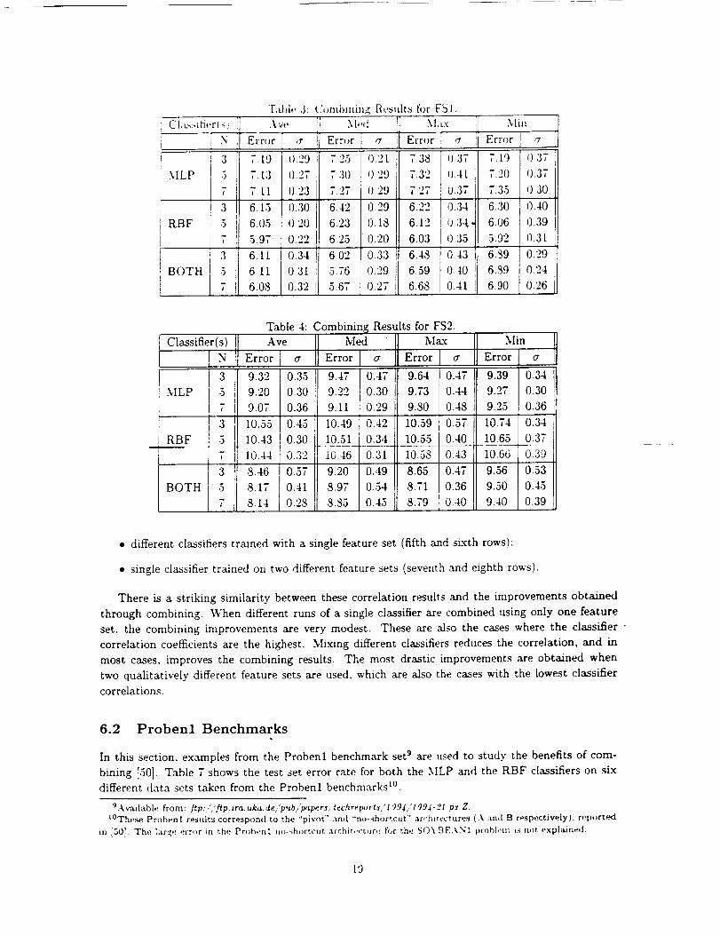
Fabb' 3: Cornbmm_ Results fi)r FSI.

Error I ,7

7.19 I).29

7.13 0.27

7. tl {).23

6.I5 0.30

6.05 0.20

5.97 O.22

6.11 0.34

6.11 0.31

6.08 0.32

,M,,,i

Err,,r i <t

725 0.21

730 029

7.27 029

6.42 0.29

6.23 0.18

6.25 020

6.02 0.33

5.76 0.29

5.67 0.27

7.38 iU.377.32 0.41

7.27 0.37

6.22 0.34

6.12 0.34

6.03 035

6.48 0.43

6.59 0.40

6.68 0.41

Min

Error! ,_i

7.19 [ (1.37

7.20 0.37

7.35 0.30

6.30 0.40

6.06 039

5.92 0.3I

6.,39 O.29

6.89 0.24

6.90 0.26

Table 4: Combining Results for FS2.

f 3 t 047 9.6 0. 7:e00e0:ee 0e0 00.22 ,0 0

I 7 . 9.25 10.36

5i- 76 s 0433 _1 8_-0 _0-49_ 8"65 10"47 9.56 10.53

_- 10"54 [I 8.71 10.36 9.50 10.45_." 0.45 8.7910.40

RBF

• different classifiers trained with a single feature set (fifth and sLxth rows):

• single classifier trained on two different feature sets (seventh and eighth rows).

There is a striking similarity between these correlation results and the improvements obtained

through combining. When different runs of a single classifier are combined using only one feature

set, the combining improvements are very modest. These are also the cases where the classifier "

correlation coefficients are the highest. Mixing different classifiers reduces the correlation, and in

most cases, improves the combining results. The most drastic improvements are obtained when

two qualitatively different feature sets are used, which are also the cases with the lowest classifier

correlations.

6.2 Probenl Benchmarks

In this section, examples from the Probenl benchmark set 9 are used to study the benefits of com-

bining [50]. Table 7 shows the test set error rate for both the MLP and the RBF classifiers on sixdifferent data sets taken from the Probenl benchmarks t°.

9Available from: fip" /,/fip.lra. uka.de/'p,tb/ p_persz techreports:'199$/z199J- 21P_ .Z.

t°These ProhenI results correspond to the "pivot" and "no-_hortcut" ar "hire,'tur_s (.k :rod B respoctively), reported

in [50[. The large error in th(.' Probent u,>-shortcut ,-trchit,,ctur(! for the S()_ BEAN1 prohh!m is not oxplaine(t.

L9

['able 8: C,>mhmmg

Cla._ifierl:) Ave ]

E,,<,rI il] 3 0.60 0.13 I

MLP 5 0.60 0.13 i7 0.60 0.13

3 1.29 0.48

RBF 5 1.26 0.47

7 1.32 /).41

3 0.86 0.39

BOTH 5 0.72 0.25

7 0.86 0.39

[/,,,_,dts _"_JrCANCER[

X[,,<t

Ert'_+t" ,7

0.63 0. I7

0.58 i).LII)

0.58 0.0()

1.1.2 0.5.3

1.12 0.47

1.18 0.43

0.63 0.18

0.72 , 0.25

0.58 I0.00

" X[_!.X Min , !IE"""rI + ' I066

063

0.60

1.90

1.81

l.Sl

1.03

1.38

1.49

02t 0.66 021

Ij.[7 0.63 0.17

0.13 0.60 0. i3

0.52 0.95 Ol2

0.53° 0.98 037

0..53 0.39 0.34

{).53 0.95 0.12

0.43 0.83 0.29

0.39 0.83 ]0.34

Table 9_in Results for CARD1.

Classifier(S_r rlaX_ a Er2lin cr

3]MLP 5

7

3[

RBF 5

7

BOTH 5

13.37 0.45 13.61 0.56 13.43 0.44 13.40 0.47

13.23 0.36 13.40 0.39 13.37 0.4.5 13.31 0.40

13.20 0.26 13.29 0.33 13.26 0.35 13.20 0.32

13.40 0.70 13.58 0.76 !i 14.01 0.66 13.08 1.05

13.11 0.60 13.29. 0.67 13.95 0.66 12.88 0.98I

13.02 0.33 12.99 0.33 1.3.75 0.76 i 12.82 0.67

13.75 0.69 13.69 0.70 13.49 0.62 13.66 0.70

13.78 0.55 13.66 0.67 13.66 0.65 13.75 0.64

13.84 0.51 13.52 0.58 13.66 0.60 13.72 0.70

The CARD 1 data set consists of credit approval decisions [51, 52]. 51 inputs are used to determine

whether or not to approve the credit card application of a customer. There are 690 examples in

this set, and 345 are used for training. The MLP has one hidden layer with 20 units, and the RBF

network has 20 kernels.

The DIABETES1 data set is based on personal data of the Pima Indians obtained from the

National Institute of Diabetes and Digestive and Kidney Diseases [63]. The binary output determines

whether or not the subjects show signs of diabetes according to the World Health Organization.

The input consists of 8 attributes, and there are 768 examples in this set, half of which are used for

training. MLPs with one hidden layer with 10 units, and RBF networks with 10 kernels are selectedfor this data set.

The GENE1 is based on intron/exon boundary detection, or the detection of splice junctions

in DNA sequences [45, 66]. 120 inputs are used to determine whether a DNA section is a donor,

an acceptor or neither. There are 3175 examples, of which 1588 are used for training. The MLP

architecture consists of a single hidden layer network with 20 hidden units. The RBF network has10 kernels.

The GLASS1 data set is based on the chemical analysis of gl_tss splinters. The 9 inputs are used

to classify 6 different types of glass. There are 214 examples in this set, antl 107 of them are used

for training. MLPs with a single hidden laver of 15 milts, and RBF networks with 20 kernels are

'2l

('l_tssiti,.r,_)i N

74

MLP _ 5

J

! 3

RBF ! 5

7

3

BOTH I 5i

[';d,l,, t2: {',,mLmln_ [{,'s_dts

32.07 0.00

32.07 0.011

32.07 0.00

29.81 2.28

29.23 1.84

29.06 1.5t

30.66 2.52

32.36 1.82

32.45 [0.96

32_)7

?,2 [17

32 07

30.76

30 I9

30.1)0

2906

28 30

2793

000

0.00

0.00

2.74

1.69

1.88

2.0'2

1.46

i 1.75

fi,r { ;[..\SSt

_ [;I,X

Err(}r ,y

,) ,1 -.,...I), 0.00

32.07 0.00

32.07 0.00

30.28 2.02

30.85 2.00

31.89 1.78

33.,87 l. 74

33.68 1.82

34. t5 ', t.68

3207 0.00

32.07 000

32.07 0.00

29.43 2.89

- 28.30 2.46

27.5.3 t.83

29.9t ] 2.2529.72 1.78

2991 1.61

SOYBEAN1.

3

MLP 5

7

13r

5

7

3

BOTH 5

_7j

RBF

7.06

7.06

7.06

7.74

7.62

7.68

7.18

7.18

7.18

0.00

0.00

0.00

0.47

0.23

0.23

0.23

0.23

0.24[

7.09

7.06

7.06

7.65

7.68

7.82

7.12

7.12

7.18

0.13

0.00

0.00

0.42

0.30

0.33

0.17

0.17

0.23

7.06 0.00

7.06 0.00

7.06 0.00

7.85 0.47

7.77 0.30

7.68 02-9

7.56 0.28

7.80 0.28

7.50 0.25

7.85 1.42

8.38 1.63

8.88 1.68

7.77 0.44

7.65 0.42

7.85 1.27

8.06 1.22

8.09 1.05

in most cases. If the combined bias is not lowered, the combiner will not outperform the better

classifier. Second. as discussed in section 5.2. the correlation plays a major role in the final reduction

factor. There are no gnarantees that using different types of classifiers will reduce the correlation

factors. Therefore. the combining of different types of classifiers, especially when their respective

performances axe significantly different (the error rate for the RBF network on the CANCER1 data

set is over twice the error rate for MLPs) has to be treated with caution.

Determining which combiner (e.g. ave or reed), or which classifier selection (e.g. multiple MLPs

or MLPs and RBFs) will perform best in a _ven situation is not generally an easy task. However,

some information can be extracted from the experimental results. The linear combiner, for example,

appears more compatible with the MLP classifiers than with the RBF networks. When combining

two types of network, the reed combiner often performs better than other combiners. One reason for

this is that the outputs that will be combined come from different sources, and selecting the largest

or smallest value can favor one type of network over another. These results emphasize the need for

closely coupling the problem at hand with a classifier/combiner. There does not seem to be a single

type of network or combiner that can be labeled "best" under all circumstances.

,)v+'rrt'n.trtm_. bizt not un(h't'tr+tmmg (exv+Ppt in <'asl,s wh+,r,, rh,' _ztt(l(,rtraintn_ is v,.rv tttthl) This

<'()I't',)]}(>r;tP(,`++'+,,il wiPh I+1|), th,,{}r,+tic;d fr;utt+,wt>t'k whi<h sh(}w_+ +'{}tttlJltting t{} be rti+}i'+,t,ff<-,{'ti,¢l, ;It

,;;).ri;)+tx_'+,r,,,l,J,:l+io[t P+h;tn F)i;us t'_'dnt<'tlou.

Tit+' <:[;_sificati(m r:ttos obtaine(I by t.he orcler +t;+tisti('s c(}ntbiners in section 6 /+re in general,

<'+>ntp_r,_ble _o r.hose obtaine_I by averaging. The advantage <)f O$ approa('h+,s sh(mld be tnore _+vi<tettt

m situations where there is substantial variability in the performance of individual classifiers, an<l the

thus robust properties of OS combining can be brought to bear upon. Such variability in individual

perfortnance may be due t,o, for exanlple, the classifiers being geographifally distributed and working

only on h>cally available data of highly varying quality. Current work by the authors mdi<:ate that

this is indeed the case, but the issue needs to be examined in greater detail.

One final note that needs to be considered is the behavior of combiners for a targe number of

classifiers (.V). Clearly, the errors cannot be arbitrarily reduced by increasing N indefinitely. This

observation however, does not contradict the results presented in this analysis. For large N, the

assumption that the errors were i.i.d, breaks down, reducing the improvements due to each extra

classifier. The number of classifiers that yield the best results depends on a number of factors,

including the number of feature sets extracted from the data, their dimensionality, and the selectionof the network architectures.

Acknowledgements: This research was supported in part by AFOSR contract F49620-93-1-0307.

NSF grant ECS 9307632, and ARO contracts DAAH 04-94-G0417 and 04-9.5-10494.

R:effevences .......

[1] K. AI-Ghoneim and B. V. K. Vijaya Kumar. Learning ranks with neural networks (Invited

paper). In Applications and Science of Artificial Neural Networks, Proceedings of the SPIE,

volume 249_'2. pages 446-464, April 1995.

[2] K. M. Aii and M. J. Pazzani. On the link between error correlation and error reduction in

decision tree ensembles. Technical Report 95-38. Department of Information and Computer

Science, University of California, Irvine, 1995.

[3] B.C. Arnold, N. Balakrishnan, and H.N. Nagaraja. A First Course in Order Statistics. Wiley,New York, 1992.

[4] J.A. Barnett. Computational methods for a mathematical theory of evidence. In Proceedings

of the Seventh International Joint Conference on Artificial Intelligence, pages 868-875, August1981.

[5] R. Battiti and A. M. Colla. Democracy in neural nets: _,bting schemes for classification. Neural

Networks, 7(4):691-709, 1994.

[6] W. G. Bazct. Improving the accuracy of an artificial neural network using multiple differently

trained networks. Neural Computation, 4:772-780, 1992.

[71 ,I.A. Benediktsson, J.R. Sveinsson, O.K. Ersoy, and P.H. Swain. Parallel consensual neural

networks with optimally weighted outputs. [n Proceedings of the World Congress on Neural

Networks, pages [II:129-137. INNS Press, 1994.

[,_3]V. Biou, .I.F Gibrat, .I.M. Levin, B. Robson, and .I Garnier. Secondary structure prediction:

combia;_tit)n of thr(.'e different metho(ls. Protew Engineering, 2:185-9l, 1988.

25

126i.I. (;h<J.'-;hart<[K ['Illnt+rStt'_u'turala_laptati<mand._+'neralizai't_mtlt ,+up,.rvl+_++,_tfl,e_lfiwvvar<l

tl_'r, work+..]ott, r+rt+al ,Jr ,,1 rt+.fic+a+ ;V++P/+ra_ +Wettuor_.+, l( l): _+_ i 4._,++ [9+)4.

[27] .l. Ghosh. [(. TItrm'r, b. B+*<'k. a.n,t L. D+,lts+,r. [nt,++_rati_m <>fn,+Ttr;d ,.l,+u.+slfi+prsfor p;u_siv++ 3<Jt,;!.r

signals. In C.T. Leondes. editor. Control and Dynwm+c S,/+tems--Adwmces :n Theor 7 and

Apphcat:on._, volume 77, pages 31)t-338+ Academic Press, 1996.

[2,.'3] C. W .1. Granger. Combining forec,'k_ts--twenty years tater. ]otLrnal of Forecastin 9. 813): 167-173, 1989.

r"

[29] J.B. Hampshire and A.H. Waibe[. The Meta-Pi network: Building distributed representations

for robust multisource pattern recognition. [EEE Transactwns on Pattern ,4nalyszs and Ma-

chine [ntellzgence. 14(7):751-769, 1992.

[30] L. K. Hansen and P. Salamon. Neural network ensembles. [EEE Transactions on Pattern

Analysis and Machine [ntellzgence, 12(10):993-1000, 1990.

[31] S. Hashem and B. Schmeiser. Approximating a function and its derivatives using MSE-optimal

linear combinations of trained feedforward neural networks. In Proceedings of the Joint Con-

ference on Neural Networks, volume 87, pages I:617-620, New Jersey, 1993.

[32] D. Heckerman. Probabilistic interpretation for MYCIN's uncertainty factors. In L.N Kanal

and J.F. Lemmer, editors, Uncertainty in Artificial intelligence+ pages 167-196. North-Holland,1986.

[3-_ TI [(. [t'-o.-.J-..I. WrI_,]], aml S. N. Srihari. De_cigi0n combination in multiple-dlassifier systems.

IEEE Transactions on Pattern Anal_tsis and Machine Intelligence, 16(1):66-76, 1994.

[34] Robert Jacobs. Method for combining experts' probability assessments. Neural Computation,7(5):867-888, 1995.

[35] A. Jain, R. Dubes, and C. Chen. Bootstrap techniques for error estimation. [EEE Transactions

on Pattern Analysis and Machine Intelligence, 9:628-633, 1987.

[36] A. Krogh and J. Vedelsby. Neural network ensembles, cross validation and active learning.

In G. Tesauro, D. S. Touretzky, and T. K. Leen, editors, Advances in Neural Information

Processing Systerna-7, pages 231-238. M.I.T. Press, 1995.

[37] J. Lee, J.-N. Hwang, D.T. Davis, and A.C. Nelson. Integration of neural networks and decision

tree classifiers for automated cytology screening. In Proceedings of the International Joint

Conference on Neural Networks, Seattle, pages I:257-262, July 1991.

[38] E. Levin, N. Tishby, and S. A. Solla. A statistical approach to learning and generalization in

layered neural networks. Proc. IEEE, 78(10):1568-74, Oct 1990.

[39] W.P. Lincoln and J Skrzypek. Synergy of clustering multiple back propagation networks. In

D. Touretzky, editor, Advataces in Neural Information Processing Systems-2, pages 650-657.Morgan Kaufmann, 1990.

[40] O. L. Mangasarian, R. Setiono, and W. H. Wolberg. Pattern recognition via linear programming:

Theory and application to medical diagnosis. In Thomas F. Coleman anti Yuying Li, editors,

Large-SoMe Nt+mer;cal Optun_zatum, pages 22-30. SIAM Publications, 1990.

2.

'.')5i (', [_l_,_jv:L (2't_lllhi[lHlg th,' r,,sutt_ ,)t srv,_r;d n,'ur;d m,t.w_rk c!;Lssifi,,rs. :V_ ual ,Vetwork._.

7_5_:777-7,'_L. it)94.

!56] [1. F_(Js+,n. Eas+_mblr lrarnLng using ,l+!c+Jrr_qate<[ m,ur,'d aet, work:+ Connectwn ,_',:t,+nce. J'p+'cml

[.s.sue on Combining .4rt+fic:al Ne'ur++l Networks. En.semble Appro,+ches, 8! 3 & 4)::373-384, 1996.

i571 D W. Rile:k+ S K. Rogers, M. E. Kabrisky, M. E. Oxley, an,l B W. Surer. The muLtilayer

P-r,'eptron as an approximation to a Bayes +JptitttaL discriminant bmction. [EEE Transactions

on Ne,+ral Networks, 1(4):296-298, 199(16

iS+l A. E. Sarhan and B+ G. Greenberg. Estimation of location and scale parameters by order

+tar, istics front singly and doubly censored samples. Annals of J,[athemat+cal Statzstzcs Science,

27:427-451, 1956.

[591

[6o]

R. Schapire, Y. Freund, P. Bartlett, and Lee W.S. Boosting the margin: A new explanation for

the effectiveness of voting methods. In Proceedings o/the Fourteenth International Conference

on Machine Learning. Morgan Kaufmann 1997.

A..l.J. Sharkey. (editor). Connection Science." Special Issue on Combining Artificial Neural

Networks." Ensemble Approaches, 8(3 & 4), 1996.

S. Shlien. Multiple binary decision tree classifiers. Pattern Recogmtion, 23(7):757-63, 1990.

PA. Shoemaker, M.J. Carlin, R.L. Shimabukuro, and C.E. Priebe. Least squares learning and

approximation of posterior probabilities on classification problems by neural network models.

In Proc. 2nd Workshop on Ne'urul Networks, WNN-AIND91,]t-u[_urTi/pa-ges 187-_9-6_-Fe-bruar_,-1991.

i631

[64]

[65]

[66]

J. W. Smith, J. E. Everhart, W. C. Dickson, W. C. Knowler. and R. S. Johannes. Using

the ADAP learning algorithm to forecast the onset of diabetes mellitus. In Proceedings of

the Symposium on Computer Applications and Medical Care, pages 261-265. IEEE Computer

Society Press, 1988.

P. Sollich and A. Krogh. Learning with ensembles: How overfitting can be useful. In D. S.

Touretzky, M. C. Mozer, and M. E. Hasselmo, editors, Advances m Neural Information Pro-

cessin9 System3-8, pages 190-196. M.I.T. Press, 1996.

M. Stone. Cross-validatory choice and assessment of statistical prediction. Journal of the Royal

Statistical Society, 36:111-147, 1974.

G. G. Towell and J. W. Shavlik. Interpretation of artificial neural networks: Mapping

knowledge-based neural networks into rules. In I.E. Moody, S.J. Hanson, and R.P. Lipl>

mann, editors, Advances in Neural Information Processing Systems-,L pages 977-984. Morgan

Kaufmann, 1992.

[67]

[6_1

[t_91

K. Turner and J. Ghosh. Limits to performance gains in combined neural classifiers. In Pro-

ceedings o[ the Artificial Neural Networks in Engineenng "95, pages 419--424, St. Louis, 1995.

K. Turner and J. Ghosh. Order statistics combiners for neural classifiers. In Proceedings of the

World Congress on :Ve.ural Networks. pages [:31-34, Washington DC.. 1995 INNS Press.

K. Timber amt .I. Ghosh. Analysis of drcision boundaries m linearly c_mlbined neural ,:la.ssifiers.

P,dh;r'n Recognmon, 29(2):3-11-348, Frbruary 1996.

29