Sensitivity of binary liquid thermal convection to confinementPublished in Physics of Fluids (2003), Vol. 15, pp. 2791-2802

E. Millour, G. LabrosseUniversite Paris-Sud,

Laboratoire d’Informatique pour la Mecanique et les Sciences de l’IngenieurLIMSI-CNRS BP 133, 91403 ORSAY CEDEX, FRANCE.

E. TricUniversite Nice Sophia Antipolis,Laboratoire Geosciences AZUR,

250 rue Albert Einstein, 06560 VALBONNE, FRANCE.

Abstract

The stable axisymmetric convective states of a binary liquid enclosed in a verti-cal cylinder heated from below are exhaustively and accurately identified by pseudo-spectral numerical integration. In order to gain some insight on the influence thatnearby boundaries can exert on flow dynamics, three aspect ratios (1/2, 1 and 2), aswell as two types of lateral kinematic boundary conditions (either no-slip or free-slip)are investigated. The ranges over which stable quiescent, oscillatory and steady con-vective states extend and coexist are given. The bifurcations leading to transitionsfrom one branch of solutions to another, as well as those that occur along the oscilla-tory branch, are analyzed. The most significant effect of varying boundary conditionsand aspect ratio involves the route from oscillatory to steady convection. For a givenconfiguration, that route consists of a period doubling cascade followed by chaos, or asubcritical generalized Hopf (or Neimark-Sacker) bifurcation, or a homoclinic bifurca-tion. The dynamics of thermal convection of enclosed binary mixtures is clearly verysensitive to both boundary conditions and aspect ratio.

1 Introduction

Since the initial investigations of Benard and Rayleigh, convection in horizontal fluid lay-ers heated from below is a problem that has been extensively studied in the context ofpattern formation, instabilities and dynamical behavior of nonlinear systems (see, for exam-ple, Cross and Hohenberg [1] an references therein). Convection in cylindrical enclosures ofaspect ratios around unity is a topic that has drawn much attention over the past years.Experimental and numerical studies of the convective flows that arise beyond onset, as wellas their secondary instabilities, are still ongoing, as exemplified by many recent publications(see, e.g., Muller, [2] Touihri et al., [3] Hof et al., [4] Leong,[5] among others). Such workstypically focus on following the evolution of flows with Rayleigh number Ra (which accountsfor the externally imposed thermal stress) in given cases (i.e. given aspect ratio Γ, fluidPrandtl number Pr and thermal boundary conditions). Despite these many contributions,the knowledge of all the solutions and bifurcations that arise in the Γ-Pr-Ra parameterspace is so far incomplete.

Investigations on thermal convection of binary fluids began about 30 years ago (see Plat-ten and Legros [6]). In these mixtures, solute mass fraction and temperature gradients arecoupled by the Soret effect. According to the sign of the Soret coefficient, the solute (whichwe take to be the heaviest of the two components) migrates towards the warmer or colderpart of the container, and an initially homogeneous mixture, once subjected to a thermalgradient, separates in composition. The resulting Soret-driven mass fraction gradient thus

1

induces a solutal buoyancy that works against or with the thermal one. Both sign and ampli-tude of the Soret coupling are accounted for in the dimensionless separation ratio ψ betweensolutal and thermal buoyancies. These compete when ψ is negative, and their interplayyields additional (compared to pure fluids in the same conditions) complex spatiotemporalbehaviors, which can moreover arise as the quiescent state turns unstable. Over the pastdecades an impressive number of 2D studies has been published on this system (see for in-stance Kolodner et al., [7] Barten et al., [8] Lucke et al., [9] and references therein), mainlyfocused on horizontally infinite or very extended layers. All point out the dynamical richnessof this configuration and confirm the extreme sensitivity of thermal flows to the presence ofsolutal distributions, even when mass fraction amplitudes are very small.

Numerical explorations of these systems are harder to carry out than when pure fluid areconsidered. The dimension of the parameter space to investigate is higher (Γ, Pr, Ra, ψ andLewis number Le). Moreover, the occurrence of time-dependent flows rising directly from therest state implies extra numerical requirements. First, their exploration must be performedover significantly large durations in order to reach settled temporal behaviors. Secondly, thenumerical scheme that is used must be consistent with the continuous space-time problemto solve.

Three-dimensional numerical simulation of the first bifurcations in binary liquid thermalconvection cannot therefore be yet considered as feasible, and literature is so far devoid ofany results of this kind. What has been done in 2D focuses on limited regions of parameterspace and mainly on large aspect ratio enclosures. To this day, even the 3D linear stabilityof a quiescent layer in small aspect ratio cylindrical cells has not been fully explored. Suchanalyses have been performed, by Hardin et al. [10] and Mercader et al., [11] but over limitedranges of parameters. The reason for this is that which mode (axisymmetrical or azimuthal)is the most destabilizing depends on all of the system’s parameters (i.e. Γ, Pr, Le and ψ).Note that the (temporal and azimuthal) structure of the destabilizing mode is not necessarilythat of the resulting non linear solution. Since it is known that in the pure fluid case, [4, 5]axisymmetrical and 3D states coexist over specific sub-domains (in Ra), such may also occurfor binary liquids.

Experiments on convection of water-ethanol mixtures in long rectangular cells (of vari-able aspect ratio, length over height of the enclosure ranging from 15 to 21) by Kolodner [12]display a strong sensitivity of flow dynamics to the length of the apparatus. This featurewas also obtained in the 2D numerical simulations of Batiste et al. [13, 14]. The presentwork tackles a specific aspect of the richness of 2D dynamics in thermal convection of abinary liquid. We analyze the non linear states that occur in axisymmetrical enclosures ofsmall aspect ratios (radius over height ratio), namely Γ = 1/2, 1 and 2, and with two typesof boundary conditions for the velocity on the circumference of the cylinder, either no-slipor free-slip. The former simply represents the presence of a rigid wall, whereas the latter isa crude approximation (capillary effects being discarded) of a straight free surface and themodeled system is then related to a liquid bridge (Wanschura et al. [15]).

From the forthcoming results, it will be inferred that thermal convection of a binaryliquid is extremely sensitive to both aspect ratio and boundary conditions.

This paper is organized as follows: the equations ruling binary liquid thermal convectionare given and discussed in Sec. 2. The numerical tool and methods used for the simula-tions are presented in Sec. 3. Results obtained for the six modeled configurations are given

2

and compared in Sec. 4, where the multitude of bifurcations that arise are detailed. Ourconclusions are then summarized in Sec. 5.

2 Physical Model

2.1 Ruling equations

The usual Oberbeck-Boussinesq equations, Soret effect included, are considered. Using theheight h of the layer, the thermal diffusion velocity over h, the imposed temperature differ-ence ∆T (between bottom and top plates) and the Soret-induced mass fraction difference∆C of the quiescent state as reference scales leads to the following set of dimensionlessequations:

∂v

∂t+ (v.∇)v = −∇p+RaPr (θ + ψγ) e

z+ Pr∇2v, (1)

∇.v = 0, (2)

∂θ

∂t+ (v.∇)θ = v.e

z+ ∇2θ, (3)

∂γ

∂t+ (v.∇)γ = v.e

z+ Le (∇2γ −∇2θ), (4)

where v = uer+ we

zis the velocity, e

rand e

zare respectively the radial and upward unit

vectors. p, θ and γ denote departures from pressure, temperature and mass fraction staticprofiles. The four numbers that appear in the governing equations are

Ra =α∆T g h3

νκ, ψ =

β∆C

α∆T, Pr =

ν

κ, Le =

D

κ,

where α and β are the (positive) thermal and solutal expansion coefficients, ν, κ and Dare the momentum, heat and mass diffusivities, g is the gravitational acceleration. The lastthree numbers are constant for a given fluid and here set to Pr = 1, Le = 0.1 and ψ = −0.2(values that roughly are those of a 3He-4He mixture [17, 16]), leaving Ra as the main pa-rameter of this study. Recall that taking ψ to be negative implies that solutal and thermalbuoyancies compete.

All boundaries are impervious to matter. Temperatures are imposed on the horizontalwalls, along with lateral thermal insulation. Top and bottom boundary conditions are:

θ =∂θ

∂z−∂γ

∂z= u = w = 0 for z = ±

1

2.

Denoting the aspect ratio Γ = R/h, where R is the radius of the cylinder, the lateralconditions on the scalar fields are:

∂θ

∂r=∂γ

∂r= 0 for r = Γ.

As previously mentioned, two sets of kinematic lateral boundary conditions are considered:

(a) No-slip: u = w = 0 for r = Γ,

or

(b) Free-slip: u =∂w

∂r= 0 for r = Γ.

In all that follows, these will be referred to as (a) NS and (b) FS configurations.

3

Nz 30 40 50 60 80 100

δE 4.210−7 1.210−8 5.410−11 2.110−12 5.110−13

δθ 2.810−5 4.610−7 5.710−9 1.110−11 4.410−11

γ 1.110−7 3.310−10 1.510−10 5.010−11 9.110−12 5.510−12

d 4.310−4 1.210−4 2.510−5 7.010−6 9.010−6 6.010−6

Table 1: Evolution of global quantities with grid size. These values were obtained for asteady flow at Ra = 3000, in the Γ = 2 NS configuration, with a time step δt of 5 10−4.Grids of (2Nz + 1) × (Nz + 1) nodes in r × z were used. δθ and δE denote the relativedifference to the overall temperature θref = −2.69562701076 10−2 and kinetic energy Eref =1.5660498335843 102 obtained as references with Nz = 100. The last two lines of the tablerefer to the mean mass fraction γ in the enclosure (γ should be zero) and the relative velocitydivergence d (see text).

2.2 Symmetries of the solutions

Since in the following sections the symmetries of both steady and time-dependent convectivestates will be of interest, we mention here that the up-down (or mirror symmetry, denotedM) in the governing equations implies the following:if X1 = (u1, w1, p1, θ1, γ1) satisfies equations (1-4), then so does X2 = (u2, w2, p2, θ2, γ2),provided that

u2(r, z, t) = u1(r,−z, t),

w2(r, z, t) = −w1(r,−z, t),

p2(r, z, t) = p1(r,−z, t),

θ2(r, z, t) = −θ1(r,−z, t),

γ2(r, z, t) = −γ1(r,−z, t).

Solutions therefore either come in pairs that transform into one another under M or areinvariant under such a transformation.

Periodic oscillations (of period τ) may possess a temporal symmetry T relating solutionsseparated by half a period in the following way:

u(r, z, t+τ

2) = u(r,−z, t),

w(r, z, t+τ

2) = −w(r,−z, t),

p(r, z, t+τ

2) = p(r,−z, t),

θ(r, z, t+τ

2) = −θ(r,−z, t),

γ(r, z, t+τ

2) = −γ(r,−z, t).

The role of temporal symmetry and its practical implications have been examined andclarified by Swift and Wiesenfeld. [18] The main result of their study is that in systems suchas the one investigated here, time-symmetric oscillations cannot undergo period doublingbifurcations. These solutions are hence typically [19] found to first bifurcate to asymmetrybefore undergoing period doubling.

4

3 Numerical method

3.1 Spatial and temporal integrations

The set of governing equations is solved by a Chebyshev pseudo-spectral method in spaceand a second-order finite-differences scheme in time.

Gauss-Lobatto nodes are used in the vertical direction ez, located at

zj = −1

2cos

(

πj

Nz

)

with j ∈ [0, Nz] ,

where Nz is the highest degree (cutoff frequency) of the Chebyshev polynomial expansion.Gauss-Radau nodes are used in the radial direction e

r, located at

rj =Γ

2

(

1 + cos

(

2π(Nr − j)

2Nr + 1

))

with j ∈ [0, Nr] .

Note that using a Gauss-Radau grid enables one to avoid the singularity at r = 0 and toimplicitly impose the axisymmetry boundary conditions on the axis, namely u = ∂w

∂r= ∂θ

∂r=

∂γ∂r

= 0.The cutoff frequencies Nr and Nz were chosen such that Nr = ΓNz, which leads to grids

of (ΓNz + 1)(Nz + 1) nodes.

Time integration is achieved by a second-order finite-differences approximation, usinga three-level scheme for time derivatives, diffusion and advection terms respectively beingevaluated implicitly and explicitly. Velocity and pressure fields are uncoupled via a specificprojection-diffusion algorithm [20, 21] which is consistent, [22] in contrast to the well knowntime-splitting schemes, with the continuous uncoupled velocity-pressure problem. Pressureis first obtained by solving a quasi-Poisson operator without having to impose any boundarycondition on this field. Velocity is then obtained by solving a standard unsteady diffusionequation with a divergence-free right hand side. Since the numerical divergence of any ana-lytically known divergence-free field cannot exactly cancel but only asymptotically with nodenumber, this approach yields, by truncation, an asymptotically solenoidal velocity. This hasbeen commented at length by Tric et al., [23] who obtained the expected exponential decreaseof ∇.v with cutoff frequencies in computations of thermally driven pure fluid convection ina cubical cavity.

3.2 Accuracy assessments

3.2.1 Spatial convergence

Using a pseudo-spectral approach leads to expect an exponential improvement of numericalsolutions with increasing cutoff frequencies. This has been checked using the following globalinstantaneous quantities:

E = 2π∫ r=Γ

r=0

∫ z=1/2

z=−1/2

v.v

2rdrdz ,

θ = 2π∫ r=Γ

r=0

∫ z=1/2

z=−1/2θ rdrdz ,

γ = 2π∫ r=Γ

r=0

∫ z=1/2

z=−1/2γ rdrdz , d =

||∇.v||

||(v.v)1/2||,

5

10-12

10-10

10-8

10-6

10-4

10-2

10 20 30 40 50 60 70

δ ω

NZ

Figure 1: Evolution of the relative error δω on the angular frequency of a time-dependentflow with grid size [(2Nz + 1) × (Nz + 1) nodes in r × z]. These values were obtained fora monoperiodic flow at Ra = 2600, in the Γ = 2, NS configuration, with a time step δt of10−3.

where ||. . .|| denotes the infinite norm (i.e: the maximum pointwise absolute value), E is thekinetic energy in the enclosure, θ and γ are the global temperature and concentration of themixture and d is the relative velocity divergence. The evolution of these four quantities withmesh size, for a given steady solution, is given in Table 1. Both γ and d must asymptoticallycancel with increasing Nz, as long as roundoff errors are not taken into account. The reasonfor this, in the case of γ, comes from solute mass conservation requirement, all boundariesbeing impervious to matter. Note that such is not the case for θ since nothing imposesthat incoming and outgoing heat fluxes should be instantaneously equal. Having no a priorivalues for θ and E to compare to, those obtained with the refined grid Nz = 100, for whichd and γ are clearly converged, are used as reference. The results given in Table 1 show theexpected exponential improvement up to at least Nz = 60, followed by saturation due toroundoff effects.

As for the convergence behavior of settled periodic solutions, Fig. 1 displays the relativeerror

δω =

∣

∣

∣

∣

∣

ω(Nz) − ω(Nz = 80)

ω(Nz = 80)

∣

∣

∣

∣

∣

on the angular frequency of a test case. Here as well, the exponential convergence withincreasing cutoff frequencies is obtained.

All forthcoming results were obtained using grids of (101 × 51), (71 × 71), (51 × 101)nodes for the Γ = 2, 1 and 1/2 configurations. Some results were cross-checked on finer gridsof (161 × 81), (111 × 111) and (81 × 161) nodes, respectively. Resulting shifts in thresholdvalues (even in regions where chaotic flows occur) were of less than 0.05%.

6

10-6

10-5

10-4

10-3

10-2

10-5

10-4

10-3

10-2

δ ω

δ t

Γ = 1 / 2Γ = 2

Figure 2: Influence of δt on δω, the relative deviation to our most accurate computations(ω = 7.19525440315 when δt = 3 10−5 for Γ = 1/2, and ω = 7.533299504778 when δt = 10−4

for Γ = 2).

3.2.2 Temporal convergence

Solutions were taken to be stationary when the following criterion was fulfilled,

Max

(

|φn+1 − φn|

|φn|

)

< 10−4δt ,

where φn stands for the value of any of the physical fields at dimensionless time nδt andMax denotes the maximum evaluated over all fields and nodes.

In the case of time-dependent solutions, a first indication of the effective time-dependencycan be extracted from inspection of Poincare section (see Sec. 4.1). When the solutionsseemed to be monoperiodic, they were deemed so when their instantaneous angular frequency(computed from the return times between successive impacts in the Poincare section) satu-rated over its first 8 significant figures.

The time step δt to be used for sufficiently accurate computations of time-dependentsolutions was estimated from several test cases such as those given in Fig. 2. The relativedeviation δω to reference ωref obtained with a “small enough” time step δt is given. Itdepicts the (expected) second-order temporal convergence of the numerical resolution. Thevalues of δt used to obtain all forthcoming results were chosen to be such that δω < 10−4 forthe previously mentioned test cases and are: δt = 3 10−4, 10−3 and 10−3 for the Γ = 1/2, 1and 2 NS configurations and δt = 2 10−4, 10−3 and 5 10−4 for the Γ = 1/2, 1 and 2 FS ones.

4 Results

Results are presented in four steps. The first is dedicated to the analysis of typical tran-sient behaviors and to informations these yield about bifurcation thresholds and types. An

7

-2

-1

0

1

2

0 20 40 60 80 100 120 140

u

t

7.5

8

8.5

9

9.5

10

0 20 40 60 80 100 120 140

ωn

t

0

0.03

0.06

0.09

0.12

0 20 40 60 80 100 120 140

wn

t

-0.015

-0.012

-0.009

-0.006

-0.003

0

0 20 40 60 80 100 120 140

θ n

t

-0.25

-0.2

-0.15

-0.1

-0.05

0

0 20 40 60 80 100 120 140

γ n

t

Figure 3: Upper row: Left plot: Evolution of the radial velocity at node P1 for Ra = 2600in the Γ = 2, NS configuration. At time t = 0 the quiescent state is perturbed by asmall random amplitude and the system evolves towards a stable periodic solution. Rightplot: Corresponding instantaneous angular frequency ωn (evaluated from return times τn inthe Poincare section, see text). Lower row: vertical velocity wn, temperature θn and massfraction γn in the Poincare section.

overview of the branches of solutions with their general characteristics is then given, followedby a presentation of the general features of the oscillatory states. Finally, the oscillatoryflows’ successive bifurcations, up to the transition to steady regimes (also known as SteadyOverturning Convection, SOC) are described.

4.1 Transient behaviors

The temporal evolution of the system is followed by monitoring the values of u, w, θ and γat a pair of z-symmetric nodes P1 and P2, located at rj=2(Nr+1)/3 and zj=(Nz+1)/3, zj=2(Nz+1)/3

respectively.

These time series provide useful information not only about the attractor that is reached(once transients associated with initial conditions die away), but also on the local bifurca-tions that occur in the system.

In the vicinity of local bifurcations, the temporal evolution about solutions is given bywell known and documented (see, e.g., the monographs of Manneville [24] or Ott [25], amongothers) normal forms. Corresponding transient evolutions are then exponentially growing ordecaying with a rate λ linked to both the type of the bifurcation and the distance to thethreshold value Racrit of the control parameter. Thus, in the case of a pitchfork bifurcation,one should have λ ∝ (Ra − Racrit), as well as for a Hopf bifurcation, where the transientwill also display oscillations. For a saddle-node bifurcation, λ2 ∝ (Ra− Racrit).

8

-0.03

-0.025

-0.02

-0.015

-0.01

-0.005

0

0.005

0.01

0.015

2574 2576 2578 2580 2582 2584 2586

λ

Ra

-0.2

-0.1

0

0.1

0.2

0.3

0.4

0.5

0.6

2625 2630 2635 2640 2645

λ2

Ra

Figure 4: Left: Temporal growth rate λ of infinitesimal perturbations of the conductive stateas a function of the Rayleigh number in the vicinity of the Hopf bifurcation of the quiescentstate (Γ = 2, NS configuration). Right: Squared temporal growth rates λ2 of transientrelaxation towards the stationary state close to the saddle-node bifurcation (Γ = 2, NSconfiguration). In both cases, the solid line is obtained using the linear law given by the twopoints that lie closest to vanishing growth rate.

The values of λ (obtained at given values of Ra) can simply be extracted from the timeseries (monitored at P1 and P2) as transients die away and the system settles towards asolution S. This procedure is rather straightforward if S is a steady state. When S is aperiodic solution, the transient evolutions from which the aforementioned behaviors are tobe extracted come from those obtained in a Poincare section. The Poincare section usedthroughout this study is build from the time series recorded at P1. It is defined by thecanceling of u, going from negative to positive values, each impact yielding (discrete) timeseries of w, θ, γ and τ (return time between successive impacts).

An illustration is given in Fig. 3. The time series depicts the evolution of u at P1, in acase where the initial condition of the system is a quiescent state (unstable at the Ra valueset for this run) perturbed (at t = 0) by an O(10−2) random amplitude. Since the quiescentsolution has turned unstable via a Hopf bifurcation, the perturbation triggers the (linear)Hopf mode. As long as amplitudes remain small (t < 70), the transient evolution of thesystem is an exponentially growing oscillation composed of a single frequency, as shown bythe plot of ωn (angular frequency evaluated from the return times between impacts in thePoincare section) in Fig. 3. When amplitudes become large, the contribution of nonlinearterms to the dynamics is no longer negligible and the system settles towards a stable peri-odic solution (t > 100). The exponential dying out of the transient, as the latter solution isreached and from which a value of λ can be extracted, is quite obvious in the plots given inFig. 3.

An example of the feasibility and limitation of following the evolution of λ with Ra inthe vicinity of a local bifurcation in order to pinpoint the threshold value from the obtainedtrends is given in Fig. 4. The expected trend (respectively linear (top) or quadratic (bottom)in the vicinities of Hopf or saddle-node bifurcations) is generally obtained over a small domainin Ra in the vicinity of the bifurcation. Obtaining the λ(Ra) trend not only proves that theinferred bifurcation indeed occurs, but yields a more accurate estimation of the threshold

9

AB CD AB CD AB CDA : 3148.5

1 NS B : 3079.5C : 3271.3D : 3011.5

A : 15167.812

NS B : 14717C : 15797.1D : 14938

A : 2582.32 NS B : 2573.2

C : 2875.7D : 2628.8

A : 8412.712

FS B : 8349C : 8948D : 8116.8A : 2434.0

1 FS B : 2430.5C : 2588.8D : 2326.5A : 2327.1

2 FS B : 2326.5C : 2551.9D : 2215.7

Table 2: Sketches of the three relative positionings of conductive, oscillatory and steadybranches of solutions. Top row: Bifurcation diagrams corresponding to the three observedcases. The horizontal line depicts the rest state, ending at a subcritical Hopf bifurcation(A). The middle curve depicts time-dependent states bounded by a saddle-node bifurcation(B) and the transition to SOC (C). The upper curve depicts steady convective states, thelower boundary of which is a saddle-node (D).

value (by definition the value of Ra for which λ cancels) than (necessarily extremely lengthy,due to critical slowing down as λ→ 0) direct simulations.

4.2 Branches of solutions

It is well known that, for binary liquids enclosed in extended containers, a sequence of allowedstates occurs as Ra is increased, starting from the quiescent state towards steady states afteran intermediate oscillatory regime. Each of these states exists over a given domain, thusleading to hysteresis in transitions from one solution to the other. The branches of stablesolutions of all the configurations investigated in this work are sketched and categorized inTable 2. Four characteristic points, along with corresponding threshold values are given: Afor the end of the rest state branch (subcritical Hopf bifurcation), B (saddle-node) and C(see Sec. 4.4), the extremities of the oscillatory branch and D (saddle-node) the beginning ofthe SOC domain. The relative positions of points A,B and D was used to categorize results:going from the leftmost to the rightmost column, point D moves from the left of B to theright of A. In all cases, taking a quiescent state to values of Ra above RaA triggers theHopf mode and leads to an oscillatory state. We find that aking an oscillatory solution toRa values lower than RaB always sends the system back to a quiescent state, even if steadyconvection is also possible for that value of Ra. This reflects the effective extension of thequiescent state’s basin of attraction. Configurations given in the leftmost column of Table 2

10

0.00 0.25 0.50

0.50

0.00

-0.50

0.00 1.00

0.50

0.00

-0.50

φmin = −0.35, φmax = −0.05 φmin = −0.8, φmax = −0.1

0.00 1.00 2.00

0.50

0.00

-0.50

φmin = −3.0, φmax = 1.0

Figure 5: Streamfunction φ contours of stationary flows for Γ = 1/2 (FS configuration,Ra = 8600), Γ = 1 (NS configuration, Ra = 3300) and Γ = 2 (FS configuration, Ra = 2550).Solid and dashed lines indicate positive and negative values (clockwise and anti-clockwisemotion) of φ. Displayed contour levels are evenly distributed and range from φmin to φmax.Note that the rolls are not even in z and that applying the mirror symmetry M to thestreamfunction is equal to transforming φ(r, z) into −φ(r,−z) .

are such that the steady state branch extends below the oscillatory one (i.e. RaD < RaB).When RaD > RaB (middle and rightmost column of Table 2), taking a steady flow to Ravalues below RaD leads to oscillatory convection. Note that for the Γ = 2, NS configu-ration (rightmost column of Table 2), oscillatory convection is the only stable solution forRaA < Ra < RaD. All FS configurations are found to belong to the same category, whereasthe NS ones span all three, non-monotonically with Γ.

The evolution of the Hopf thresholds of the rest state (point A in Table 2) with aspectratio, as well as that of the corresponding Hopf marginal frequencies (given on the plots inTable 3), agree with linear stability results: [10, 11]

1. the values increase slightly from Γ = 2 to 1 and, obviously, much more dramaticallywhen Γ < 1;

2. they increase as well going from FS to NS conditions.

Moreover, these trends also hold for all the thresholds of both oscillatory and steady flows.

11

Before going into a detailed description of the oscillatory branches, we mention here thatthe steady convective states’ characteristics, in the range of Ra values considered, are verysimilar for a given aspect ratio (1 roll for Γ = 1 and 1/2 and a pair of rolls for Γ = 2) andnot sensitive to the choice of boundary conditions. Figure 5 depicts typical flow structuresfor Γ = 1/2, 1 and 2. All SOC solutions do not possess the M symmetry property andtherefore always come in M-symmetric pairs.

4.3 General features of the oscillatory states

Table 3 depicts the angular frequencies of all the monoperiodic oscillatory states, for all Γand both types of boundary conditions. Going along these curves with increasing Ra valuescorresponds to following the oscillatory branches of Table 2, from point B up to point C inthe NS case or up to the last monoperiodic flow in the FS one.Point C is not given for the FS configurations in Table 3 as the oscillatory states turnaperiodic before the transition to SOC. These will be described in Sec. 4.4.3. Of the sixinvestigated configurations, only two (Γ = 1 and Γ = 1/2, NS) are such that the frequencyof the oscillations goes to zero as the transition to SOC is reached.

All time dependent states which stem from B share the temporal symmetry T . Only inthe Γ = 2, NS configuration is it found to hold over the entire oscillatory domain. In allother configurations, this symmetry breaks down, at point T . This occurs via a supercriticalpitchfork bifurcation at the Ra (= RaT ) values given in Table 4. The emerging pair ofperiodic solutions are M-symmetric. The proportion of the oscillatory domain over which Tholds is found to increase with Γ in both the FS and NS configurations, which could implythat Γ needs to be smaller than a critical value in order to break the T symmetry. Anothereffect, apparently also due to the highly constrained geometry of the enclosure, appears fromthe inspection of the last column of Table 4: the overlap between stable quiescent and os-cillatory branches decreases with respect to the oscillatory domain’s extension as Γ increases.

The next section deals with the description of the specific bifurcations that occur in eachof the six investigated configurations.

4.4 Successive bifurcations of the oscillatory flows

4.4.1 Γ = 2, NS configuration

As mentioned in the previous section, in the Γ = 2, NS configuration, no temporal symmetrybreaking occurs. The branch of oscillatory solutions terminates in this case via a subcriticalgeneralized (or secondary) Hopf bifurcation. As Ra is increased towards the bifurcationvalue, the monoperiodic solutions display transient decaying oscillatory modulations. Anexample of the evolution of resulting impacts in the Poincare section given in Fig. 6 where

an embedding of the values of w at the (n+1)th impact versus the nth is shown. The {w(n+1), w(n)} sets spiral in towards a final value, according to both growth rate λ and angularfrequency of the secondary Hopf mode. The evolution of λ in the vicinity of this bifurcationis given in Fig. 6. At the bifurcation, the secondary Hopf frequency is 0.61, roughly adecade lower than the oscillation’s base frequency. Increasing Ra slightly beyond RaC ,the corresponding monoperiodic solution turns unstable with an initially small modulationarising and growing exponentially. Since the bifurcation is subcritical, the amplitude of themodulation does not saturate (no matter how close to RaC Ra may be) and the system isenventually cast towards the nearby stable SOC solutions.

12

NS FS

0

3

6

9

12

15

18

14800 15000 15200 15400 15600 15800

ω

Ra

ωHopf = 28.84

C

T

6

8

10

12

14

16

18

20

8400 8500 8600 8700 8800 8900

ω

Ra

ωHopf = 24.87

T

0

1

2

3

4

5

6

7

8

3100 3150 3200 3250

ω

Ra

ωHopf = 10.44

C

T

3

4

5

6

7

8

9

2450 2475 2500 2525 2550 2575

ω

Ra

ωHopf = 9.623

T

5

6

7

8

2600 2650 2700 2750 2800 2850

ω

Ra

ωHopf = 9.123

C

3

4

5

6

7

8

9

2325 2375 2425 2475 2525

ω

Ra

ωHopf = 8.794

T

Table 3: Angular frequencies of monoperiodic flows. Top row: Γ = 1/2, middle row: Γ = 1,lower row: Γ = 2. Points T and C, when given, indicate the occurrence of temporal symmetrybreaking and the transition to SOC (see Table 2).

4.4.2 Γ = 1 and 1/2, NS configurations

The Γ = 1 and 1/2 configurations have much in common. As previously mentioned, theseare the only cases for which the frequency of the oscillations is found to go to zero as thetransition to SOC is reached.

As might be guessed from the cluster of points near the end of the oscillatory branchesgiven in Table 3, quite distinctive behaviors occur there. An enlargement of the end ofthe oscillatory branch (Γ = 1/2 case) is given in Fig. 7, showing that there are in fact two

13

Case RaTRaT −RaB

RaC−RaB

RaA−RaB

RaC−RaB

12

(SF) 8900.5 0.921 0.1061 (SF) 2577.9 0.931 0.02212 (SF) 2542.2 0.957 0.0026612

(NS) 15619.7 0.836 0.4171 (NS) 3260.3 0.943 0.3602 (NS) - - 0.0301

Table 4: Rayleigh number values at which temporal symmetry T is broken (second column),proportion of the oscillatory domain over which T holds (third column) and over which bothoscillatory and conductive states are stable (fourth column).

0.68

0.681

0.682

0.683

0.684

0.685

0.686

0.687

0.688

0.689

0.68 0.681 0.682 0.683 0.684 0.685 0.686 0.687 0.688 0.689

w(n

+1)

w(n)

-0.14

-0.12

-0.1

-0.08

-0.06

-0.04

-0.02

0

0.02

0.04

2855 2860 2865 2870 2875 2880

λ

Ra

Figure 6: Left: Embedding of the successive values of the vertical velocity w in the Poincaresection, depicting the transient modulation of the periodic state (here, the Ra = 2875 flow)by the secondary Hopf mode in the Γ = 2, NS configuration. w(n) is the value at the nthimpact. As time (and therefore n) increases, the {w(n+ 1),w(n)} sets spiral in toward theirfinal value, w(n + 1) = w(n) = 0.6841. Right: Temporal growth rates λ of the transientmodulation of the periodic state as a function of the Rayleigh number, close to the generalizedHopf bifurcation (the solid line is obtained using the linear law given by the two points thatlie closest to vanishing growth rate).

branches which overlap over a very narrow range in Ra. Since the upper branch ends ina saddle-node bifurcation and the lower branch begins at one, we conjecture that they aredirectly connected to each other by an unstable part (obviously unaccessible to our timemarching process). Such “bending” of the periodic states branch leading to the coexistenceof two stable oscillatory states has also been numerically observed (in mixtures for whichPr = 10 and Le = 0.01) in extended layers, [9] when Ψ < −0.4.

Another important feature depicted in Fig. 7 is the extremely sharp drop in frequencythat occurs at the end of the lower branch.

Does the frequency go down to zero as the bifurcation is reached? Such is the case, asindicated by Fig. 8, where the period τ = 2π/ω versus the distance Ra − RaC is plotted,with RaC = 15797.0099.

The data match a τ ∝ − ln (RaC − Ra) scaling law which meets one of the behaviorsobtained in horizontally infinite plane layers (see Knobloch, [26] Knobloch and Moore [27]).

14

0

1

2

3

4

5

6

7

15780 15785 15790 15795

ω

Ra

Figure 7: Angular frequencies of periodic solutions at the end of the oscillatory domain, inthe Γ = 1/2, NS configuration.

1.4

1.6

1.8

2

2.2

2.4

2.6

2.8

1e-05 0.0001 0.001 0.01 0.1 1 10

τ

Ra - RaC

Figure 8: Period τ of the oscillations versus the distance (Ra − RaC , where RaC ≃15797.0099 ) to the homoclinic bifurcation of the periodic orbit (Γ = 1/2, NS configura-tion).

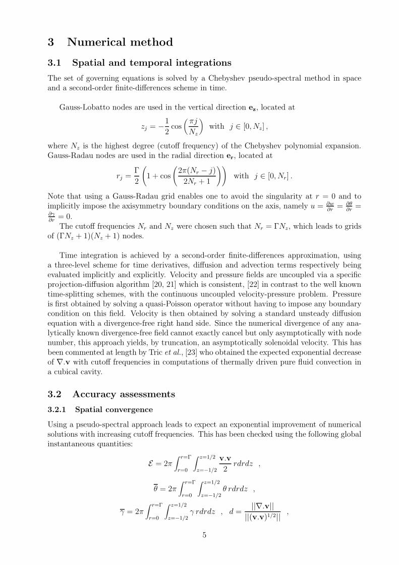
In the latter, the transition corresponds to a standing waves branch vanishing in a heteroclinicbifurcation between the limit cycle and a pair of steady state solutions. In the present case,the limit cycle collides with an unstable SOC fixed point in a homoclinic bifurcation whichleads to the same scaling. An illustration of this global bifurcation is given in Fig. 9 wherephase portraits of the limit cycle prior to the bifurcation and the path followed by the systemafterwards are shown.

In unbounded layers, another possible scenario involves traveling waves (TW), the fre-

15

-0.35

-0.25

-0.15

-0.12 -0.06 0

γ

θ

-2 0 2

-0.35

-0.25

-0.15

-5

0

5

-2 0 2

w

u

-5

0

5

-0.12 -0.06 0

Figure 9: Projections of the phase portrait of the periodic orbit (full line) in the (θ, γ), (u, γ),(u, w) and (θ, w) planes, prior (Ra = 15797.0098) to the homoclinic bifurcation. The arrowsindicate the direction of motion along the orbit. The large dot depicts the initial positionof the system when Ra was increased to Ra = 15797.0099, slightly above RaC . From thatpoint, the system first closely follows the path given by the limit cycle, up to an outset thatsends it off (dashed line) towards the stable SOC fixed point (star).

quency of which also vanishes as SOC is reached, but following a τ ∝ (RaTWC −Ra)−1/2 law.

It corresponds to a collision between a group orbit (of SOC solutions, each being neutrallystable with respect to translation) and isolated TW solutions.

This homoclinic bifurcation of the oscillatory branch also occurs in the Γ = 1 case. Theonly difference between the Γ = 1 and Γ = 1/2, NS configurations is that the branch bendingthat arises in the latter does not occur in the former.

4.4.3 FS configuration

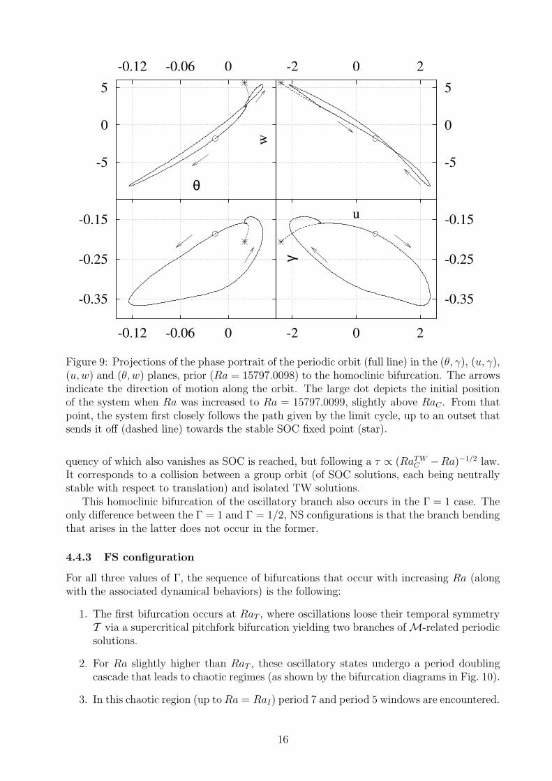
For all three values of Γ, the sequence of bifurcations that occur with increasing Ra (alongwith the associated dynamical behaviors) is the following:

1. The first bifurcation occurs at RaT , where oscillations loose their temporal symmetryT via a supercritical pitchfork bifurcation yielding two branches of M-related periodicsolutions.

2. For Ra slightly higher than RaT , these oscillatory states undergo a period doublingcascade that leads to chaotic regimes (as shown by the bifurcation diagrams in Fig. 10).

3. In this chaotic region (up toRa = RaI) period 7 and period 5 windows are encountered.

16

-0.36

-0.34

-0.32

-0.3

-0.28

2543 2545 2547 2549 2551

RaT I C

-0.34

-0.33

-0.32

-0.31

-0.3

8905 8915 8925 8935 8945

RaT I C

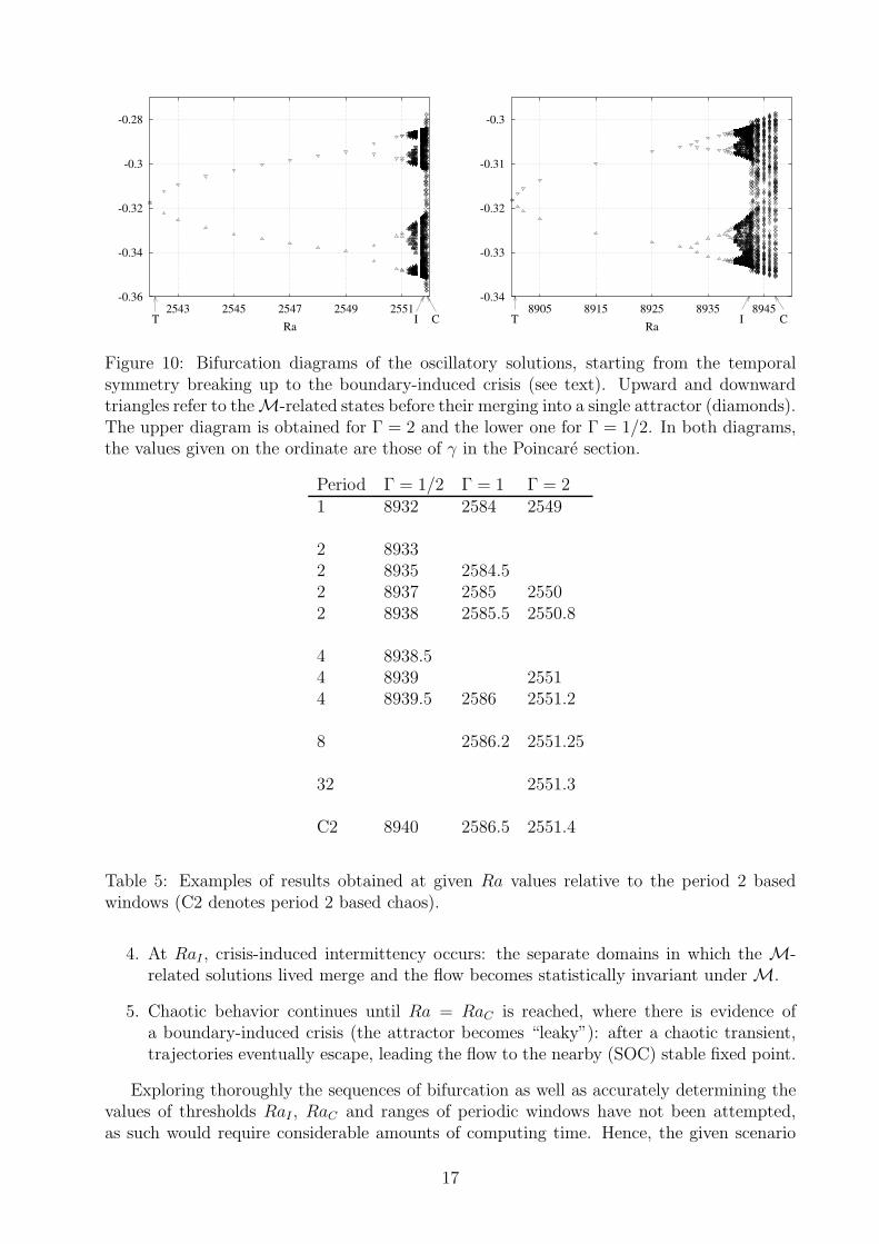
Figure 10: Bifurcation diagrams of the oscillatory solutions, starting from the temporalsymmetry breaking up to the boundary-induced crisis (see text). Upward and downwardtriangles refer to the M-related states before their merging into a single attractor (diamonds).The upper diagram is obtained for Γ = 2 and the lower one for Γ = 1/2. In both diagrams,the values given on the ordinate are those of γ in the Poincare section.

Period Γ = 1/2 Γ = 1 Γ = 21 8932 2584 2549

2 89332 8935 2584.52 8937 2585 25502 8938 2585.5 2550.8

4 8938.54 8939 25514 8939.5 2586 2551.2

8 2586.2 2551.25

32 2551.3

C2 8940 2586.5 2551.4

Table 5: Examples of results obtained at given Ra values relative to the period 2 basedwindows (C2 denotes period 2 based chaos).

4. At RaI , crisis-induced intermittency occurs: the separate domains in which the M-related solutions lived merge and the flow becomes statistically invariant under M.

5. Chaotic behavior continues until Ra = RaC is reached, where there is evidence ofa boundary-induced crisis (the attractor becomes “leaky”): after a chaotic transient,trajectories eventually escape, leading the flow to the nearby (SOC) stable fixed point.

Exploring thoroughly the sequences of bifurcation as well as accurately determining thevalues of thresholds RaI , RaC and ranges of periodic windows have not been attempted,as such would require considerable amounts of computing time. Hence, the given scenario

17

-0.4

-0.39

-0.38

-0.37

-0.4 -0.39 -0.38 -0.37

γ n+

1

γn

-0.4

-0.39

-0.38

-0.37

-0.4 -0.39 -0.38 -0.37

γ n+

1

γn

Figure 11: γn+1 vs γn Poincare section return map (from the Γ = 1, FS configuration),displaying the attracting sets before (upwards and downwards triangles, Ra = 2586.78) andafter (diamonds, Ra = 2587.5) the occurrence of crisis-induced intermittency.

is inferred from obtained results and comparison with typical results detailed in mono-graphs [25, 24] on dynamical systems. For the sake of completeness, we give the followingexamples:

• In all cases period 2 behavior is indeed found to be followed by period 4, but as theperiod doubling cascade continues, it does so in a very narrow range in Ra, and in-termediate doublings were sometimes missed (see Table 5). A closer look at Poincaresection return maps (such as the ones shown in Fig. 11), along with successive embed-dings thereof, shows that, even though the maps are not unimodal, they evolve verymuch as the standard logistic map does (greater differences do arise beyond the period2 window). From that, we conjecture that the period doubling cascade is probablycomplete in all three configurations.

• Similarly, the statement that period 5 and 7 windows occur comes from the combinedexamination of return maps and results such as landing in one (for instance, period 5behavior is found at Ra = 8942 for Γ = 1/2 and period 10 occurs at Ra = 2586.79 forΓ = 1) or witnessing related chaotic behavior (at Ra = 2586.8 for Γ = 1 as well as atRa = 2551.725 for Γ = 2).

It might be worth mentioning here a series of numerical investigations [28, 19, 29] ondoubly diffusive convection (in which the Soret effect is neglected and a vertical mass fractiongradient is externally imposed) in 2D Cartesian enclosures of small lateral extension. Inthese boxes, oscillatory solutions were found to exhibit a rich variety of spatiotemporalbehaviors, such as multiple coexisting branches of “bubble” structure (cascades of perioddoubling bifurcations leading to chaos and followed by reverse sequences which restore simpleperiodicity). These studies, in which temporal symmetry breaking followed by a cascade ofperiod doubling bifurcations leading to chaotic oscillations is observed, were obtained withfree-slip boundary conditions.

5 Conclusions

In this paper, axisymmetric convection of a binary liquid enclosed in a vertical cylinder isinvestigated. In order to clarify the influence of nearby side boundaries on flow dynamics,

18

three aspect ratios (Γ = 2, 1 and 1/2), as well as either no-slip or free-slip boundary condi-tions on the cylinder’s circumference, are considered.

The oscillatory states are found to undergo various and multiple bifurcations, the oc-currences of which strongly depend on the choice of both boundary conditions and aspectratio. The most significant difference between NS and FS configurations lies in the route toSOC: The oscillatory branches of solutions of NS cases terminate via either a homoclinic (forΓ = 1/2, 1) or a subcritical generalized Hopf (or Neimark-Sacker) bifurcation (for Γ = 2),whereas those of the FS cases undergo a period doubling cascade, followed by chaos. It isknown [18] that the latter route can only occur for states not possessing the T symmetry.Moreover, the proportion of the oscillatory domain over which T does not hold is found todecrease with increasing Γ, much faster in NS than in FS configurations (Table 4). It canthus be conjectured that either all FS cases do bifurcate to SOC in the same way (meaningthat the proportion shrinks, but only asymptotically, with Γ), or that there is a criticalaspect ratio beyond which the route to SOC will be different. The NS configuration is anobvious illustration of the existence of such a critical aspect ratio Γcrit (about 1.3 from thedata in Table 4). Below Γcrit, T -symmetry breaking occurs: it does not however lead toperiod doubling but to a (global) homoclinic bifurcation, as the limit cycle collides with anunstable SOC fixed point. Above Γcrit, it is a (local) subcritical Hopf bifurcation of theT -symmetrical monoperiodic solutions that leads to SOC.

The dynamical richness of this system is such that some details (e.g. the very smallRa ranges of hysteretic features) are likely to escape experimental investigations, even ifextremely carefully designed.

The presence of nearby side boundaries clearly induces significant changes in the dynam-ical behavior of binary liquid thermal convection.

acknowledgments

We gratefully acknowledge the Centre de Ressources Informatiques de l’Universite Paris-Sudfor granting us unbounded use of their computer facilities.

References

[1] M. C. Cross and P. C. Hohenberg, “Pattern formation outside of equilibrium,” Rev.Mod. Phys. 65, 851 (1993).

[2] U. Muller, “Convection in cylindrical containers at supercritical Rayleigh numbers,”PHYSICA D 97, 180 (1996).

[3] R. Touihri, H. Ben Hadid, and D. Henry, “On the onset of convective instabilities incylindrical cavities heated from below. I. Pure thermal case,” Phys. Fluids 11, 2078(1999).

[4] B. Hof, P. G. J. Lucas, and T. Mullin, “Flow state multiplicity in convection,” Phys.Fluids 11, 2815 (1999).

[5] S. S. Leong, “Numerical study of Rayleigh-Benard convection in a cylinder,” Numer.Heat Transfer, Part A 41, 673 (2002).

[6] J. K. Platten and J. C. Legros, Convection in Liquids (Springer Verlag, Berlin, 1984).

19

[7] P. Kolodner, S. Slimani, N. Aubry, and R. Lima, “Characterization of dispersive chaosand related states of binary-fluid convection,” PHYSICA D 85, 165 (1995).

[8] W. Barten, M. Lucke, M. Kamps, and R. Schmitz, “Convection in binary fluid mixture.I. Extended traveling-wave and stationary states,” Phys. Rev. E 51, 5636 (1995).

[9] M. Lucke, W. Barten, P. Buchel, C. Futterer, C. Hollinger, and CH. Jung, “Patternformation in binary fluid convection and in systems with throughflow,” in Evolution of

structures in dissipative continuous systems, edited by F. H. Busse and S. C. Muller(Springer, 1998).

[10] G. R. Hardin, R. L. Sani, D. Henry, and B. Roux, “Buoyancy-driven instability in avertical cylinder: binary fluids with Soret effect. Part I: general theory and stationarystability results,” Int. J. Numer. Methods Fluids 10, 79 (1990).

[11] I. Mercader, M. Net, and E. Knobloch, “Binary fluid convection in a cylinder,” Phys.Rev. E 51, 339 (1995).

[12] P. Kolodner, “Repeated transients of weakly nonlinear traveling-wave convection,”Phys. Rev. E 47, 1038 (1993).

[13] O. Batiste, I. Mercader, M. Net, and E. Knobloch, “Onset of oscillatory binary fluidconvection in finite containers,” Phys. Rev. E 59, 6730 (1999).

[14] O. Batiste, M. Net, I. Mercader, and E. Knobloch, “Oscillatory binary fluid convectionin large aspect-ratio containers,” Phys. Rev. Lett. 86, 2309 (2001).

[15] M. Wanschura, H. C. Kuhlmann, and H. J. Rath, “ Three-dimensional instability ofaxisymmetric buoyant convection in cylinders heated from below,” J. Fluid Mech. 326,399 (1996).

[16] R. P. Behringer, “Rayleigh-Benard convection and turbulence in liquid helium,” Rev.Mod. Phys. 57, 657 (1985).

[17] G. W. T. Lee, P. Lucas, and A. Tyler, “Onset of Rayleigh-Benard convection in binaryliquid mixtures of 3He in 4He,” J. Fluid Mech. 135, 235 (1983).

[18] J. W. Swift and K. Wiesenfeld, “Suppression of period doubling in symmetric systems,”Phys. Rev. Lett. 52, 705 (1984).

[19] E. Knobloch, D. R. Moore, J. Toomre, and N. O. Weiss, “Transitions to chaos in two-dimensional double-diffusive convection,” J. Fluid Mech. 166, 409 (1986).

[20] A. Batoul, H. Kallouf, and G. Labrosse, “Une methode de resolution directe (pseu-dospectrale) du probleme de Stokes 2D/3D instationnaire. Application a la cavite en-trainee carree,” C. R. Acad. Sci. Paris 319, 1455 (1994).

[21] G. Labrosse, E. Tric, H. Khallouf, and M. Betrouni, “A direct (pseudo-spectral) solverof the 2D/3D Stokes problem: transition to unsteadiness of natural-convection flow ina differentially heated cubical cavity,” Numer. Heat Transfer, Part B 31, 261 (1997).

[22] E. Leriche and G. Labrosse, “High-order direct Stockes solvers with or without tem-poral splitting: numerical investigations of their comparative properties,” SIAM J. Sci.Comput. 22, 1386 (2000).

20

[23] E. Tric, G. Labrosse, and M. Betrouni, “A first incursion into the 3D structure of nat-ural convection of air in a differentially heated cubical cavity, from accurate numericalsolutions,” Int. J. Heat Mass Transfer 43, 4043 (2000).

[24] P. Manneville, Dissipative Structures and Weak Turbulence (Academic, San Diego,1990).

[25] E. Ott, Chaos in Dynamical Systems (Cambridge University Press,1993).

[26] E. Knobloch, “Oscillatory convection in binary mixtures,” Phys. Rev. A 34, 1538 (1986).

[27] E. Knobloch and D. R. Moore, “Minimal model of binary fluid convection,” Phys. Rev.A 42, 4693 (1990).

[28] H. E. Huppert and D. R. Moore, “Nonlinear double-diffusive convection,” J. Fluid Mech.78, 821 (1976).

[29] D. R. Moore, N. O. Weiss, and J. M. Wilkins, “Asymmetric oscillations in thermosolutalconvection,” J. Fluid Mech. 233, 561 (1991).

21