SEMINAIRE BOURBAKI´ VOLUME 1999/2000 EXPOSES 865-879´
440
AST ´ ERISQUE 276 S ´ EMINAIRE BOURBAKI VOLUME 1999/2000 EXPOS ´ ES 865-879 Soci´ et´ e Math´ ematique de France 2002 Publi´ e avec le concours du Centre National de la Recherche Scientifique
Transcript of SEMINAIRE BOURBAKI´ VOLUME 1999/2000 EXPOSES 865-879´
ASTERISQUE 276
SEMINAIRE BOURBAKIVOLUME 1999/2000EXPOSES 865-879
Societe Mathematique de France 2002Publie avec le concours du Centre National de la Recherche Scientifique

!" #
Mots clefs et classification mathématique par sujets (2000)
! " #$
! % & ' ( )*
) + )
) , , -
K*'. . / . ) *
. !0. 1 ' ) G* 2
3 . 4*5 / $ 6
'. 7*! 1 / 89" ' ) .
, : 2;, 2;< #" #=
-& >*- K*' 5
T ;0;; " #
=' ' &
! *!) - 20 -2
" ' *
# # 2
3 / . /
? ' & 9 28
- 5 ' 9 ) )
2 "
! 4 ) !0. *
2" 22
3 3 ) @ '. )
' > ># >; #=2 21 21
" A' ' ' ' . 22
# 2 2
8. ) A A' . *
0*'. ;9 A
> > >!B* !;;
< . 8
/ $ 0

SEMINAIRE BOURBAKIVOLUME 1999/2000
EXPOSES 865-879
Résumé. — ! $ % &" '() * + " " ( , ,) - , ,% " , (% ., " % " $ ,) ( ) / ' "#
Abstract (Séminaire Bourbaki, volume 1999/2000, exposés 865-879) ( , $ / ( - ( -/ $'
/ + 0 , (' - , ( / , ,' 0 / ( ,' ( ., 0 1 % , (' ' / #
© $ / A!


TABLE DES MATIERES 1
Resumes des exposes . . . . . . . . . . . . . . . . . . . . . . . . . . . . . . . . . . . . . . . . . . . . . . . . . . . . . . . . 3
NOVEMBRE 1999
865 Christian KASSEL — L’ordre de Dehornoy sur les tresses . . . . . . . . . . 7
866 Jean-Francois LE GALL — Exposants critiques pour le mouvementbrownien et les marches aleatoires [d’apres Kenyon, Lawler etWerner ] . . . . . . . . . . . . . . . . . . . . . . . . . . . . . . . . . . . . . . . . . . . . . . . . . . . . . . . . . . 29
867 Miles REID — La correspondance de McKay . . . . . . . . . . . . . . . . . . . . . . . . 53
868 Tristan RIVIERE — Ginzburg-Landau Vortices: the static model . . 73
869 Georges SKANDALIS — Progres recents sur la conjecture de Baum–Connes. Contribution de Vincent Lafforgue . . . . . . . . . . . . . . . . . . . . . . 105
MARS 2000
870 Elisabeth BOUSCAREN — Theorie des modeles et conjecture deManin-Mumford [d’apres Ehud Hrushovski ] . . . . . . . . . . . . . . . . . . . . . . 137
871 Bas EDIXHOVEN — Rational elliptic curves are modular [after Breuil,Conrad, Diamond and Taylor ] . . . . . . . . . . . . . . . . . . . . . . . . . . . . . . . . . . . . 161
872 Viatcheslav KHARLAMOV — Varietes de Fano reelles [d’apresC. Viterbo] . . . . . . . . . . . . . . . . . . . . . . . . . . . . . . . . . . . . . . . . . . . . . . . . . . . . . . . . 189
873 Gerard LAUMON — La correspondance de Langlands sur les corps defonctions [d’apres Laurent Lafforgue] . . . . . . . . . . . . . . . . . . . . . . . . . . . . 207
874 Eduard LOOIJENGA — Motivic measures . . . . . . . . . . . . . . . . . . . . . . . . . . 267
JUIN 2000
875 Edward FRENKEL — Vertex algebras and algebraic curves . . . . . . . . 299
876 Stephen S. KUDLA — Derivatives of Eisenstein series and generatingfunctions for arithmetic cycles . . . . . . . . . . . . . . . . . . . . . . . . . . . . . . . . . . . . 341
877 Teimuraz PIRASHVILI — Polynomial functors over finite fields [afterFranjou, Friedlander, Henn, Lannes, Schwartz, Suslin] . . . . . . . . . . 369
878 Vladimir TURAEV — Faithful linear representations of the braid groups. . . . . . . . . . . . . . . . . . . . . . . . . . . . . . . . . . . . . . . . . . . . . . . . . . . . . . . . . . . . . . . . . . . . 389
879 Pierre VAN MOERBEKE — Random matrices and permutations,matrix integrals and integrable systems . . . . . . . . . . . . . . . . . . . . . . . . . . . . 411
SOCIETE MATHEMATIQUE DE FRANCE 2002

RESUMES DES EXPOSES 3
Christian KASSEL – L’ordre de Dehornoy sur les tressesAu debut des annees 1990 Dehornoy a deduit un ordre total sur le groupe des tresses d’Ar-
tin a partir de l’etude generale des systemes autodistributifs, definis comme des ensemblesmunis d’une loi de composition verifiant l’identite x(yz) = (xy)(xz). Cette etude avait etemotivee par un axiome indemontrable de theorie des ensembles impliquant l’existence d’unsysteme autodistributif remarquable. Dans ce texte on presente les travaux de Dehornoy ainsique leur lien inattendu avec la theorie des ensembles. On expose aussi deux constructionsgeometriques recentes de l’ordre de Dehornoy.
Jean-Francois LE GALL – Exposants critiques pour le mouvement brownien et les marchesaleatoires [d’apres Kenyon, Lawler et Werner ]
Nous discutons certains travaux recents qui etudient les exposants critiques pour le mouve-ment brownien et les marches aleatoires. Dans la premiere partie, nous decrivons les resultatsde Lawler et Werner donnant des informations precises sur les exposants d’intersection brow-niens. Dans la seconde, nous presentons les travaux de Kenyon qui conduisent au calcul exactde l’exposant de croissance pour la marche aleatoire a boucles effacees dans le plan.
Miles REID – La correspondance de McKayLet M be a quasiprojective algebraic manifold with KM = 0 and G a finite automorphism
group of M acting trivially on the canonical class KM ; for example, a subgroup G of SL(n, )acting on
n in the obvious way. We aim to study the quotient variety X = M/G and itsresolutions Y → X (especially under the assumption that Y has KY = 0) in terms of G-equivariant geometry of M . At present we know 4 or 5 quite different methods of doing this,taken from string theory, algebraic geometry, motives, moduli, derived categories, etc.
For G in SL(n, ) with n = 2 or 3, we obtain several methods of cobbling together a basisof the homology of Y consisting of algebraic cycles in one-to-one correspondence with theconjugacy classes or the irreducible representations of G.
Tristan RIVIERE – Ginzburg-Landau Vortices: the static modelWe study the formation of vortices (zero sets having a “topological charge”) for critical
points of the Ginzburg-Landau Functional arising in the physics of supraconductivity andmore generally in abelian gauge theory. We present results regarding the existence or nonexistence of vortices in the fundamental state, their location in space and the eventual for-mation of Abrikosov lattices. We will establish a link between the position of the vorticesand the total space of solutions in the strongly repulsive limit.
Georges SKANDALIS – Progres recents sur la conjecture de Baum–Connes. Contributionde Vincent Lafforgue
Cet expose, a la suite de celui de Pierre Julg en 1998, fait un nouveau point sur laconjecture de Baum-Connes. Une nouvelle barriere vient en effet juste d’etre franchie parV. Lafforgue : celle de la propriete T de Kazhdan. Le but ici est d’exposer les diverses etapesdu travail de Lafforgue.
SOCIETE MATHEMATIQUE DE FRANCE 2002
4 RESUMES DES EXPOSES
Elisabeth BOUSCAREN – Theorie des modeles et conjecture de Manin-Mumford [d’apresEhud Hrushovski ]
Nous presenterons des applications recentes de la theorie des modeles a des questions degeometrie diophantienne sur les corps de nombres. Nous indiquerons en particulier commentE. Hrushovski, en utilisant la theorie des corps algebriquement clos munis d’un automor-phisme, donne une nouvelle demonstration de la conjecture de Manin-Mumford, demonstra-tion qui produit de bonnes bornes effectives.
Bas EDIXHOVEN – Rational elliptic curves are modular [after Breuil, Conrad, Diamondand Taylor ]
In 1994, Wiles and Taylor-Wiles proved that every semistable elliptic curve over Q ismodular, in the sense that it is a quotient of the jacobian of some modular curve. Thisresult has since then been generalized by an increasing sequence of groups of authors,culminating in the proof by Breuil, Conrad, Diamond and Taylor that all elliptic curvesover Q are modular. Their strategy is essentially that of Wiles, but they have to overcomemany technical problems. Especially the deformation theory of local Galois representationsbecomes much harder.
Viatcheslav KHARLAMOV – Varietes de Fano reelles [d’apres C. Viterbo]Les varietes de Fano sont les varietes a fibre anticanonique ample. Elles sont dominees
par des familles de courbes rationnelles. Un cas particulier d’une conjecture de J. Kollaraffirme que la partie reelle d’une variete de Fano definie sur et de dimension superieure atrois n’admet aucune metrique a courbure strictement negative. Utilisant des methodes degeometrie symplectique, C. Viterbo a montre cette conjecture dans le cas particulier ou b2 = 1et la variete est dominee par des courbes rationnelles d’aire minimale : en etudiant le flotde Floer, il montre comment l’existence de courbes rationnelles entraıne celle de geodesiquesfermees d’indice non nul sur la partie reelle.
Gerard LAUMON – La correspondance de Langlands sur les corps de fonctions [d’apresLaurent Lafforgue]
Laurent Lafforgue a etabli la correspondance de Langlands pour GLr sur un corps defonctions. Sa preuve suit la strategie introduite, il y a plus de 25 ans, par V. Drinfeld pourtraiter le cas r = 2. Une des innovations principales est la construction d’une compactifi-cation toroıdale de PGLn+1
r / PGLr pour n arbitraire qui generalise la compactification deC. De Concini et C. Procesi (n = 1).
Dans l’expose oral nous presenterons le theoreme de L. Lafforgue et ses consequences,ainsi que quelques aspects de sa tres longue demonstration (pres de 700 pages).
Eduard LOOIJENGA – Motivic measuresKontsevich proposed a Haar measure on k[[t]], k a field of characteristic zero, with values
in a universal ring that is obtained in a simple manner from the varieties over k: it assignsto the ideal tnk[[t]] the value −n , where stands for the affine line over k. This leads to ameasure with the same value ring for schemes over k[[t]]. Denef & Loeser and Batyrev haveshown that this measure gives rise to invariants with remarkable properties. These are neweven in case the scheme is obtained from a k-variety by base change.
ASTERISQUE 276

RESUMES DES EXPOSES 5
Edward FRENKEL – Vertex algebras and algebraic curvesVertex algebras are algebraic objects that formalize the concepts of vertex operators and
operator product expansion which originated from physics. They were defined by Borcherdsand studied extensively in the last fifteen years. After giving the definition of vertex algebraand describing a few examples, we show how to attach to a vertex algebra a geometric object:a vector bundle on a formal disc equipped with a flat connection and a canonical horizontalsection. We then associate to a vertex algebra and an algebraic curve an invariant called thespace of conformal blocks. These spaces reflect the geometric structure of various modulispaces associated to algebraic curves.
Stephen S. KUDLA – Derivatives of Eisenstein series and generating functions for arithmeticcycles
In their classic work, Hirzebruch and Zagier showed that certain generating functionswhose coefficients are the cohomology classes of curves on Hilbert modular surfaces are theq–expansions of elliptic modular forms of weight 2. In this talk I will describe an analogousfamily of generating functions whose coefficients arise from arithmetical algebraic geometry,e.g., from 0–cycles on the arithmetic surfaces associated to Shimura curves. The identificationof such a function with the derivative of a Siegel–Eisenstein series at its center of symmetryprovides a kind of arithmetic analogue of the Siegel–Weil formula.
Teimuraz PIRASHVILI – Polynomial functors over finite fields [after Franjou, Friedlander,Henn, Lannes, Schwartz, Suslin]
For finite fields there is an essential difference between polynomial maps and polynomials.This yields two different versions of polynomial endofunctors of finite vector spaces. Thefirst one is closely related to unstable modules over Steenrod algebra, while the second one isrelated to representations of algebraic groups. Recent works by Betley, Franjou, Friedlander,Suslin and others lead to a comparaison theorem between associated Ext-groups. Theseresults are a key for the solutions of Betley-Pirashvili conjecture involving the stable K-theory of Waldhausen and for computation of cohomology of the general linear group overfinite fields with twisted coefficients.
Vladimir TURAEV – Faithful linear representations of the braid groupsRecently D. Krammer and S. Bigelow showed that a certain homomorphism of the group
of braids on n strings Bn to a group of real matrices is injective for all n ≥ 1. This answersin the positive the long-standing question of linearity of Bn. We shall discuss these resultsof D. Krammer and S. Bigelow as well as earlier results of J. Moody (1991) and others onthe non-faithfulness of the classical Burau representation of Bn.
Pierre VAN MOERBEKE – Random matrices and permutations, matrix integrals and inte-grable systems
This lecture present a survey of recent developments in the area of random matrices(finite and infinite) and random permutations. These probabilistic problems suggest matrixintegrals (or Fredholm determinants), which arise very naturally as integrals over the tangentspace to symmetric spaces, as integrals over groups and finally as integrals over symmetricspaces. Upon apropriately adding time-parameters, these matrix integrals are natural tau-functions for integrable lattices, like the Toda, Pfaff and Toeplitz lattices, but also forintegrable PDE’s, like the Korteweg-de Vries equation. These matrix integrals or Fredholmdeterminants also satisfy Virasoro constraints, which combined with the integrable equationslead to (partial) differential equations for the original probabilities.
SOCIETE MATHEMATIQUE DE FRANCE 2002


Seminaire BOURBAKI Novembre 199952e annee, 1999-2000, no 865, p. 7 a 28
L’ORDRE DE DEHORNOY SUR LES TRESSES
par Christian KASSEL
Une des decouvertes recentes les plus interessantes et inattendues concernant legroupe des tresses Bn d’Artin est due a Dehornoy qui a demontre fin 1991 que Bn
a un ordre total invariant par multiplication a gauche. Il en resulte notamment quel’anneau du groupe Bn n’a pas de diviseurs de zero. Dehornoy deduit cet ordre del’etude generale des systemes autodistributifs, definis comme des ensembles munisd’une loi de composition verifiant l’identite x(yz) = (xy)(xz). Des travaux sur unaxiome indemontrable de theorie des ensembles avaient mis en evidence un systemeautodistributif remarquable et suggere que l’etude de tels systemes devait donner desresultats non triviaux.
Fenn, Greene, Rolfsen, Rourke et Wiest ont donne en 1997 une construction geo-metrique de l’ordre de Dehornoy. Leurs techniques ont permis egalement de mettredes structures d’ordre sur des groupes de diffeotopies de surfaces. Plus recemment,Thurston a indique comment construire un ordre total sur Bn en utilisant les travauxde Nielsen sur les surfaces.
Le but de cet expose est de presenter ces travaux ainsi que le lien inattendu avecla theorie des ensembles. Au no 1 nous enoncons le resultat principal sur l’ordre destresses et quelques proprietes de cet ordre. Les deux numeros suivants sont consacresa une presentation des techniques de Dehornoy et a sa demonstration du resultatprincipal ; le lien entre tresses et systemes autodistributifs est expose au no 2 tandisqu’au no 3 nous etudions deux systemes autodistributifs particulierement importants.Au no 4 nous indiquons comment l’etude des grands cardinaux en theorie des ensem-bles a ete a l’origine de ces travaux. La construction geometrique de Fenn et al. ainsique l’approche a la Nielsen seront presentees au no 5. Pour plus de details, le lecteurpourra consulter les references citees, et notamment la monographie [D00].
Thomas Delzant m’a aide a comprendre l’idee de Thurston et a mettre le no 5.2 enforme. Je le remercie tres chaleureusement ainsi que Patrick Dehornoy, Dale Rolfsenet Bertold Wiest qui m’ont fait profiter de leurs commentaires.
SOCIETE MATHEMATIQUE DE FRANCE 2002

8 C. KASSEL
1. LES RESULTATS PRINCIPAUX
Dans ce numero nous rappelons la definition des groupes de tresses et celle desgroupes ordonnables avant d’enoncer le theoreme principal de Dehornoy impliquantl’existence d’un ordre sur les tresses.
1.1. Le groupe des tresses d’Artin
Soit n un entier≥ 2. Definissons Bn comme le groupe engendre par n−1 generateursσ1, . . . , σn−1 soumis aux relations
(1.1) σiσj = σjσi
si |i− j| > 1 et
(1.2) σiσjσi = σjσiσj
si |i− j| = 1. On utilisera souvent le mot tresse pour designer un element de Bn.E. Artin a introduit le groupe Bn dans les annees 1920 et a resolu le probleme
des mots(1) pour ce groupe (voir [A26], [A47]). En 1967 Garside [Ga] resout a la foisce probleme et le probleme de conjugaison(1) (voir aussi [Mk]). D’autres solutionsont ete proposees, fondees notamment sur une forme normale due a Adyan [Ad],et redecouverte un peu plus tard par ElRifai et Morton [EM] et par Thurston, cedernier elaborant a cette occasion la theorie des groupes automatiques et etablissantl’automaticite de Bn (les resultats de Thurston sont exposes au chapitre 9 de [E+]).Rappelons aussi que les groupes de tresses jouent un role important dans des branchesdes mathematiques aussi diverses que la theorie des nœuds, la theorie de l’homotopie,la geometrie algebrique, la theorie des groupes, celle des representations, etc. (on trou-vera un reflet de cette diversite dans [B+] et dans [Ca]).
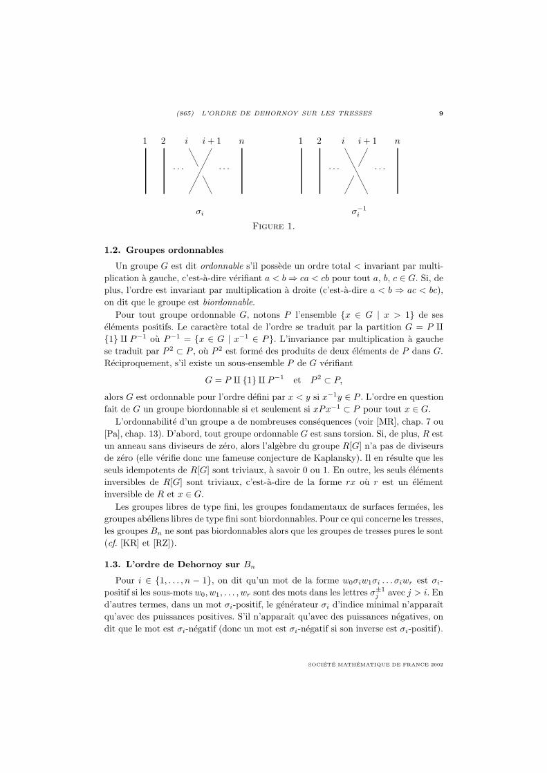
Un mot de tresse w est un mot forme a partir des generateurs σ1, . . . , σn−1 et deleurs inverses. Il est commode de representer w par une configuration plane formeepar n intervalles, appeles les brins de w, plonges de maniere lisse dans une bandeverticale bornee du plan. Une telle configuration s’obtient comme suit.
(a) On represente le generateur σi et son inverse σ−1i par les configurations de la
figure 1. Le croisement de la configuration de σi (resp. de σ−1i ) est dit positif (resp.
negatif).(b) Si D est la configuration associee au mot w et D′ celle du mot w′, alors la
configuration associee a ww′ est obtenue en placant D au-dessus de D′ et en joignantles extremites inferieures des brins de D aux extremites superieures de D′.
(1)Resoudre le probleme des mots (resp. le probleme de conjugaison) dans un groupe, c’est trouver
un algorithme permettant de reconnaıtre ou de decider si deux mots donnes representent ou non le
meme element dans le groupe (resp. la meme classe de conjugaison).
ASTERISQUE 276
(865) L’ORDRE DE DEHORNOY SUR LES TRESSES 9
· · · · · ·
1 2 i i + 1 n
σi
· · · · · ·
1 2 i i + 1 n
σ−1i
Figure 1.
1.2. Groupes ordonnables
Un groupe G est dit ordonnable s’il possede un ordre total < invariant par multi-plication a gauche, c’est-a-dire verifiant a < b⇒ ca < cb pour tout a, b, c ∈ G. Si, deplus, l’ordre est invariant par multiplication a droite (c’est-a-dire a < b ⇒ ac < bc),on dit que le groupe est biordonnable.
Pour tout groupe ordonnable G, notons P l’ensemble x ∈ G | x > 1 de seselements positifs. Le caractere total de l’ordre se traduit par la partition G = P 1 P−1 ou P−1 = x ∈ G | x−1 ∈ P. L’invariance par multiplication a gauchese traduit par P 2 ⊂ P , ou P 2 est forme des produits de deux elements de P dans G.Reciproquement, s’il existe un sous-ensemble P de G verifiant
G = P 1 P−1 et P 2 ⊂ P,
alors G est ordonnable pour l’ordre defini par x < y si x−1y ∈ P . L’ordre en questionfait de G un groupe biordonnable si et seulement si xPx−1 ⊂ P pour tout x ∈ G.
L’ordonnabilite d’un groupe a de nombreuses consequences (voir [MR], chap. 7 ou[Pa], chap. 13). D’abord, tout groupe ordonnable G est sans torsion. Si, de plus, R estun anneau sans diviseurs de zero, alors l’algebre du groupe R[G] n’a pas de diviseursde zero (elle verifie donc une fameuse conjecture de Kaplansky). Il en resulte que lesseuls idempotents de R[G] sont triviaux, a savoir 0 ou 1. En outre, les seuls elementsinversibles de R[G] sont triviaux, c’est-a-dire de la forme rx ou r est un elementinversible de R et x ∈ G.
Les groupes libres de type fini, les groupes fondamentaux de surfaces fermees, lesgroupes abeliens libres de type fini sont biordonnables. Pour ce qui concerne les tresses,les groupes Bn ne sont pas biordonnables alors que les groupes de tresses pures le sont(cf. [KR] et [RZ]).
1.3. L’ordre de Dehornoy sur Bn
Pour i ∈ 1, . . . , n − 1, on dit qu’un mot de la forme w0σiw1σi . . . σiwr est σi-positif si les sous-mots w0, w1, . . . , wr sont des mots dans les lettres σ±1
j avec j > i. End’autres termes, dans un mot σi-positif, le generateur σi d’indice minimal n’apparaıtqu’avec des puissances positives. S’il n’apparaıt qu’avec des puissances negatives, ondit que le mot est σi-negatif (donc un mot est σi-negatif si son inverse est σi-positif).
SOCIETE MATHEMATIQUE DE FRANCE 2002

10 C. KASSEL
Une tresse est dite σi-positive (resp. σi-negative) si elle peut etre representee par unmot σi-positif (resp. σi-negatif). Par exemple, le mot σ1σ2σ
−N1 n’est pas σ1-positif
si N est un entier ≥ 1, mais la tresse qu’il represente l’est (le montrer !).Nous dirons qu’une tresse est σ-positive (resp. σ-negative) s’il existe un entier i
tel qu’elle est σi-positive (resp. σi-negative). On peut alors enoncer le theoreme deDehornoy.
Theoreme 1.1. — Toute tresse differente de 1 est soit σ-positive, soit σ-negative.
La demonstration de ce theoreme occupera les numeros 2 et 3. Celui-ci a pourconsequence les resultats nouveaux suivants non connus anterieurement.
Corollaire. — (a) Pour tout n, le groupe Bn est ordonnable.(b) Pour tout n et tout anneau R sans diviseurs de zero, l’algebre R[Bn] du
groupe Bn n’a pas de diviseurs de zero, ni d’unites ou d’idempotents non triviaux.
Demonstration. — (a) Soit P l’ensemble des tresses σ-positives de Bn. Il est clair queP 2 est inclus dans P . Le theoreme 1.1 implique Bn = P 1 P−1. Il en resulteque Bn est ordonnable.
(b) C’est une consequence de (a) et des remarques faites au no 1.2.
1.4. Proprietes
L’ordre de Dehornoy ainsi defini est l’unique ordre total de Bn invariant par multi-plication a gauche tel que β σ1 β′ > 1 pour tous les elements β, β′ du sous-groupede Bn engendre par σ2, . . . , σn−1. Dans [D97b] Dehornoy a construit un algorithme deresolution du probleme des mots fonde sur l’ordre total des tresses. En pratique, cetalgorithme est beaucoup plus efficace que les algorithmes anterieurs (mais le problemereste ouvert de montrer qu’il est quadratique).
Soit B+n le sous-monoıde de Bn constitue des tresses representees par des pro-
duits des generateurs σ1, . . . , σn−1, mais non de leurs inverses. Laver [L96] a montreque l’ordre de Dehornoy prolonge l’ordre partiel considere par ElRifai et Mortondans [EM] ; il en deduit le resultat remarquable suivant, qui distingue probablementcet ordre parmi les ordres de Bn mentionnes au no 5.2.
Theoreme 1.2. — L’ordre de Dehornoy restreint a B+n est un bon ordre.
Rappelons qu’un ordre total sur un ensemble E est un bon ordre si toute partie de E
a un element minimal. Dans un bon ordre, chaque element a un rang ; par exemple,le generateur σn−1 de B+
n est le plus petit element > 1. Comme tout element de Bn
possede une ecriture canonique comme fraction de deux elements de B+n (voir [E+]),
le theoreme de Laver permet de specifier une tresse a l’aide d’un couple d’ordinaux.Burckel [Bu] a donne une autre preuve du theoreme 1.2 et montre que le type del’ordre de B+
n est ωωn−2, ou ω designe le plus petit ordinal infini. Voir aussi l’article
de Wiest [W] base sur la definition geometrique de l’ordre de Bn presentee au no 5.1.
ASTERISQUE 276
(865) L’ORDRE DE DEHORNOY SUR LES TRESSES 11
2. COLORIAGE DES TRESSES ET SYSTEMESAUTODISTRIBUTIFS
Le but du no 2 est d’indiquer comment Dehornoy demontre le theoreme 1.1.
2.1. Comment colorier les tresses ?
L’idee n’est pas nouvelle ; elle a notamment ete utilisee par Joyce [Joy], Mat-veev [Mt] et Brieskorn [Br] dans les annees 1980. Partons d’un mot de tresse w
representant un element de Bn. Colorions de gauche a droite les extremites supe-rieures des brins de la configuration plane associee a w avec les elements a1, a2, . . . , an
d’un ensemble S. Si nous propageons ces couleurs le long des brins, nous lirons aubas de la configuration une suite de couleurs qui est une permutation de la suitea1, a2, . . . , an de depart : c’est evidemment la permutation sous-jacente a la tresse.
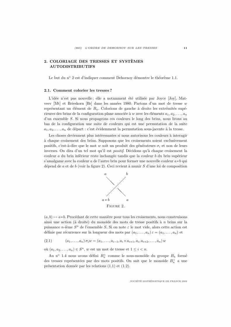
Les choses deviennent plus interessantes si nous autorisons les couleurs a interagira chaque croisement des brins. Supposons que les croisements soient exclusivementpositifs, c’est-a-dire que le mot w soit un produit des generateurs σi et non de leursinverses. On dira d’un tel mot qu’il est positif. Decidons qu’a chaque croisement lacouleur a du brin inferieur reste inchangee tandis que la couleur b du brin superieurs’amalgame avec la couleur a de l’autre brin pour former une nouvelle couleur a∗b quidepend de a et de b (voir la figure 2). Ceci revient a munir S d’une loi de composition
a b
a ∗ b a
Figure 2.
(a, b) → a∗b. Procedant de cette maniere pour tous les croisements, nous construisonsainsi une action (a droite) du monoıde des mots de tresse positifs a n brins sur lapuissance n-ieme Sn de l’ensemble S. Si on note ε le mot vide, alors cette action estdefinie par recurrence sur la longueur des mots par (a1, . . . , an) ε = (a1, . . . , an) et
(2.1) (a1, . . . , an)σiw = (a1, . . . , ai−1, ai ∗ ai+1, ai, ai+2, . . . , an)w
ou (a1, a2, . . . , an) ∈ Sn, w est un mot de tresse et 1 ≤ i < n.
Au no 1.4 nous avons defini B+n comme le sous-monoıde du groupe Bn forme
des tresses representees par des mots positifs. On sait que le monoıde B+n a une
presentation donnee par les relations (1.1) et (1.2).
SOCIETE MATHEMATIQUE DE FRANCE 2002

12 C. KASSEL
Lemme 2.1. — La formule (2.1) definit une action du monoıde B+n sur Sn si et
seulement si, pour tout a, b, c ∈ S, on a
(AD) a ∗ (b ∗ c) = (a ∗ b) ∗ (a ∗ c).
Demonstration. — On se ramene aux calculs suivants ou a, b, c, d designent deselements de l’ensemble S. Le premier calcul reflete la relation (1.1) :
(a, b, c, d)σ1σ3 = (a ∗ b, a, c ∗ d, c) = (a, b, c, d)σ3σ1.
La relation non triviale (1.2) montre la necessite de l’identite (AD) :
(a, b, c)σ1σ2σ1 =((a ∗ b) ∗ (a ∗ c), a ∗ b, a
),
(a, b, c)σ2σ1σ2 =(a ∗ (b ∗ c), a ∗ b, a
).
Definition. — Un systeme autodistributif (ou encore un systeme AD) est un en-semble muni d’une loi de composition verifiant la relation (AD) du lemme 2.1.
Par la suite, on utilisera les notions evidentes de morphisme de systemes AD, desous-systeme AD, de partie generatrice d’un systeme AD.
2.2. Ensembles automorphes
Dans ce numero, nous donnons des exemples de systemes autodistributifs. Il s’agitici de ce que Brieskorn [Br] a appele des ensembles automorphes, a savoir des sys-temes autodistributifs pour lesquels les multiplications a gauche b → a ∗ b sont bijec-tives (ces systemes particuliers ont egalement ete utilises sous d’autres noms, comme« wrack » chez Conway et Wraith, « rack » chez Fenn et Rourke [FR], « crystal » chezKauffman [Kau] ; on trouvera dans [FR] une introduction historique aux ensemblesautomorphes).
Si S est un ensemble automorphe, alors l’action de B+n sur Sn, qui est a valeurs
dans un ensemble de bijections, s’etend en une action du groupe Bn tout entier. Onobtient ainsi une methode systematique de construction de representations de Bn,methode dont les exemples (a) et (b) ci-dessous montrent l’interet.
(a) (Conjugaison) Tout groupe G est muni d’une structure de systeme AD dont laloi de composition ∗ est definie par a ∗ b = aba−1 ou a, b ∈ G.
Si G est le groupe libre Fn sur n generateurs x1, . . . , xn, posons (y1, . . . , yn) =(x1, . . . , xn)β pour tout β ∈ Bn La correspondance (x1, . . . , xn) → (y1, . . . , yn) definitun automorphisme β de Fn. L’application β → β−1 est l’homomorphisme injectif degroupes Bn → Aut(Fn) bien connu (voir par exemple [BZ], chap. 10).
(b) (Barycentre) L’anneau Z[t, t−1] des polynomes de Laurent a coefficients en-tiers a une structure de systeme AD avec a ∗ b = (1 − t)a + tb ou a, b ∈ Z[t, t−1].L’action lineaire de B+
n sur Z[t, t−1]n s’etend en un homomorphisme de groupesBn → GLn(Z[t, t−1]) : c’est la representation de Burau.
Les ensembles automorphes pour lesquels a ∗ a = a pour tout a, comme dans lesexemples (a) et (b), ont ete appeles « quandles » par Joyce [Joy] et « distributive
ASTERISQUE 276

(865) L’ORDRE DE DEHORNOY SUR LES TRESSES 13
groupoids » par Matveev [Mt] (tous deux ont utilise ce type de systemes AD pourclassifier les nœuds dans R3). Voici deux autres exemples d’ensembles automorphes.
(c) (Systemes de racines) Les vecteurs non nuls d’un espace vectoriel euclidienforment un ensemble automorphe : si a et b sont non nuls, on definit a ∗ b commel’image de b par la symetrie orthogonale par rapport a l’hyperplan orthogonal a a. Enparticulier, tout systeme de racines est un ensemble automorphe.
(d) Si l’on note FX le groupe libre engendre par les elements d’un ensemble X , onpeut munir l’ensemble-produit BX = FX ×X d’une loi autodistributive par
(w1, x1) ∗ (w2, x2) = (w1x1w−11 w2, x2)
ou w1, w2 ∈ FX et x1, x2 ∈ X . Le systeme BX est un ensemble automorphe libre ;tout ensemble automorphe S est quotient de BX ou X est une partie generatrice de S.
2.3. Cycles et acyclicite
Si a et b sont des elements d’un systeme autodistributif S, nous dirons que a diviseb (a gauche) s’il existe c ∈ S tel que b = a ∗ c. Un cycle est une suite (a1, . . . , ak)d’elements de S tels que ai divise ai+1 pour tout i < k et ak divise a1. On dit qu’unsysteme AD est acyclique s’il ne possede pas de cycle. Un ensemble automorphe n’estpas acyclique puisque tout element se divise lui-meme.
L’observation suivante montre l’interet des systemes acycliques. Sur un systemeautodistributif S on peut definir une relation binaire ≺ comme suit : a ≺ b s’il existeun entier k ≥ 1 et des elements a1, . . . , ak de S tels que a1 = a, ak = b et ai diviseai+1 pour tout i < k. La relation ≺ est transitive, et c’est une relation d’ordre partielsi S est acyclique. Avant les travaux de theorie des ensembles exposes au no 4, on neconnaissait pas d’exemple de systeme acyclique.
Proposition 2.2. — Il existe des systemes autodistributifs acycliques.
Demonstration. — Il suffit d’exhiber un exemple. Voici celui de Larue [La] qui utilisel’image dans les automomorphismes d’un groupe libre de l’operation sur les tressesque nous decrirons au no 3.3. Soit F∞ le groupe libre sur une infinite denombrablede lettres x1, x2, . . . et Aut(F∞) le groupe de ses automorphismes de groupe. Nousallons munir Aut(F∞) d’une loi autodistributive ∗. Soit α l’automorphisme de F∞determine par
α(xi) =
⎧⎪⎪⎨⎪⎪⎩x1x2x
−11 si i = 1,
x1 si i = 2,
xi si i > 2,
et T0 l’endomorphisme de F∞ donne par T0(xi) = xi+1 pour tout i ≥ 0. Ce dernierpermet de definir l’endomorphisme T de Aut(F∞) par les formules T (ϕ)(x1) = x1 etT (ϕ)(xi) = T0(ϕ(xi−1)) si i > 1 et ϕ ∈ Aut(F∞). Pour ϕ et ψ ∈ Aut(F∞), posons
(2.2) ϕ ∗ ψ = ϕ T (ψ) α T (ϕ−1).
SOCIETE MATHEMATIQUE DE FRANCE 2002

14 C. KASSEL
On verifie par un calcul direct que la loi de composition ∗ est autodistributive.
Nous affirmons que le systeme (Aut(F∞), ∗) est acyclique. En effet, soit E l’en-semble des elements de F∞ dont l’expression reduite en les generateurs x1, x2, . . . etleurs inverses se termine par x−1
1 . On observe d’abord que α, ainsi que tout elementϕ ∈ Aut(F∞) qui est dans l’image du decalage T , preserve le sous-ensemble E. Suppo-sons maintenant que le systeme Aut(F∞) possede un cycle. Cette hypothese se traduitpar une egalite de la forme ϕ = ϕ T (ϕ0) α T (ϕ1) · · · T (ϕk−1) α T (ϕk), ouk ≥ 1 et ϕ, ϕ0, . . . , ϕk−1, ϕk sont des automorphismes de F∞. De maniere equivalente,on a
(2.3) id = T (ϕ0) α T (ϕ1) · · · T (ϕk−1) α T (ϕk)
ou id represente l’automorphisme identite de F∞. Appliquons les deux membresde (2.3) a l’element x1 de F∞. A gauche, on obtient x1 qui n’appartient pas ausous-ensemble E. Par contre, comme (α T (ϕk))(x1) = α(x1) = x1x2x
−11 appartient
a E, il resulte de l’observation ci-dessus que l’element de F∞ obtenu en appliquant lemembre de droite de (2.3) a x1 appartient a E. D’ou une contradiction.
2.4. Retournement des mots
Nous avons vu au no 2.1 comment definir une action du monoıde B+n sur la puis-
sance n-ieme d’un systeme AD S et au no 2.2 que cette action s’etend au groupeBn tout entier si (et seulement si) S est un ensemble automorphe. Or, a la vue desremarques faites au no 2.3 et des travaux dont nous parlerons au no 4, la question sepose d’etendre l’action du monoıde B+
n a Bn lorsque S est acyclique. En developpantune methode specifique, dite de retournement des mots, Dehornoy a reussi a definirune action partielle de Bn sur Sn lorsque S est un systeme AD simplifiable (a gauche),c’est-a-dire un systeme pour lequel les multiplications a gauche sont injectives.
On dit qu’un mot de tresse w se transforme par retournement (a gauche) en lemot w′ si w′ s’obtient en remplacant dans w des facteurs du type σiσ
−1j par le mot
vide si i = j, par σ−1j σi si |i− j| > 1, et par σ−1
j σ−1i σjσi si |i− j| = 1. Par definition
du retournement, w et w′ representent le meme element dans Bn.
Garside [Ga] avait demontre que toute tresse est le quotient de deux tresses repre-sentees par des mots de tresse positifs. Dehornoy reprend les ingredients de l’approchede Garside, mais travaille sur les mots de tresse plutot que sur les tresses, ce qui luipermet d’etablir dans [D97a] le resultat plus fin suivant.
Lemme 2.3. — Tout mot de tresse se transforme par retournement en un mot de laforme u−1v ou u et v sont des mots de tresse positifs.
Remarquons qu’il n’est pas evident a priori que l’algorithme de retournementconverge en un nombre fini d’etapes car la longueur des mots peut augmenter a chaque
ASTERISQUE 276

(865) L’ORDRE DE DEHORNOY SUR LES TRESSES 15
retournement ; on pourra observer ce phenomene sur le mot σ2σ4σ6σ−15 σ−1
3 σ−11 . Signa-
lons que des techniques analogues de retournement des mots permettent la cons-truction de formes normales et de structures automatiques pour d’autres groupesdont les groupes d’Artin de groupe de Coxeter fini (voir [D98], [DP]).
Soit maintenant S un systeme AD simplifiable et n un entier ≥ 2. L’action adroite (a, w) → aw du monoıde B+
n sur le produit Sn, donnee par la formule (2.1),se prolonge a certains elements (a, w) de Sn×Bn de facon que les regles de coloriagerestent verifiees. C’est par exemple le cas de (bu, u−1) avec b ∈ Sn et u ∈ B+
n . Dansce cas, on dira que l’element aw est defini.
Lemme 2.4. — Soit S un systeme AD simplifiable et a ∈ Sn. Si le mot de tresse w
se transforme par retournement en w′ et si aw′ est defini, alors aw est defini.
Les lemmes 2.3 et 2.4 impliquent la proposition suivante selon laquelle on peuttoujours trouver un ensemble de couleurs dans un systeme AD simplifiable pour colo-rier une tresse donnee en suivant la regle enoncee au no 2.1.
Proposition 2.5. — Soit S un systeme AD simplifiable. Pour tout mot de tresse w,il existe a ∈ Sn tel que aw soit defini. Si w et w′ representent la meme tresse et queaw et aw′ soient definis, alors aw = aw′.
Demonstration. — Contentons-nous d’etablir la premiere assertion. D’apres le lem-me 2.3, w se transforme par retournement en w′ = u−1v ou u et v sont des motspositifs. Posons a = bu ou b est n’importe quel element de Sn. Alors aw′ = bv estdefini. On termine en appliquant le lemme 2.4.
Pour etablir la seconde assertion, on utilise une version a droite du retournementdes mots de tresse et l’hypothese que le systeme est simplifiable.
2.5. Demonstration du theoreme 1.1
Supposons que nous disposions d’un systeme autodistributif S acyclique et mono-gene (c’est-a-dire engendre par un seul element) tel que l’ordre ≺ associe (defini auno 2.3) soit total. On verifie que a ≺ b implique c ∗ a ≺ c ∗ b, d’ou l’on deduit que S
est simplifiable.Puisque S possede un ordre total, on peut munir chaque puissance Sn de S de
l’ordre total lexicographique ≺ defini par (a1, . . . , an) ≺ (b1, . . . , bn) s’il existe i ≥ 1tel que aj = bj pour tout j < i et ai ≺ bi. Nous utilisons l’ordre total ≺ sur Sn pourdefinir une partie « positive » P de Bn comme suit. Si w est un mot de tresse, alors,d’apres la proposition 2.5, il existe a ∈ Sn tel que aw soit defini. Nous dirons que latresse representee par w est dans P si a ≺ aw.
Proposition 2.6. — Une tresse est dans P si et seulement si elle est σ-positive. Larelation β < β′ definie sur Bn par β−1β′ ∈ P est une relation d’ordre total invariantpar multiplication a gauche, qui coıncide avec l’ordre de Dehornoy du no 1.3.
SOCIETE MATHEMATIQUE DE FRANCE 2002

16 C. KASSEL
Demonstration. — Montrons que, si un mot de tresse est σ-positif, alors il representeune tresse du sous-ensemble P defini ci-dessus. Un mot σi-positif w est de la formew = w0σiw1σi . . . σiwk ou w0, w1, . . . , wk sont des mots dans les lettres σj et σ−1
j
avec j > i. Soit a = (a1, . . . , an) ∈ Sn tel que aw = (b1, . . . , bn) ∈ Sn soit defini.La formule (2.1) implique que bj = aj pour tout j < i et que bi est de la formebi = (· · · ((a1 ∗ c1)∗ c2)∗ · · · )∗ ck ou c1, c2, . . . , ck ∈ S et k est le nombre d’occurrencesde σi dans w. Par definition de l’ordre≺ de S, il en resulte que ai ≺ bi. Par consequent,a ≺ aw et w ∈ P .
La reciproque, a savoir qu’une tresse dans P est σ-positive, utilise la notion detresse speciale que nous introduirons au no 3.3 et sera demontree au no 3.4.
Une fois l’equivalence precedente etablie, il est clair que la relation < est biendefinie et que c’est l’ordre total du no 1.3, dont l’existence est ainsi demontree.
3. SYSTEME AUTODISTRIBUTIF LIBRE ET TRESSESSPECIALES
Nous etudions maintenant deux systemes autodistributifs particuliers. Le premierest libre et fournit le type de systemes necessaires a la demonstration du theoreme 1.1,telle qu’elle est donnee au no 2.5. Le second est constitue de tresses.
3.1. Le systeme autodistributif libre sur un generateur
Il est caracterise par la propriete universelle suivante.
Proposition 3.1. — Il existe un systeme autodistributif D1 engendre par un single-ton x tel que, pour tout systeme autodistributif S et tout element s de S, il existeun unique morphisme f : D1 → S de systemes AD verifiant f(x) = s. Le systeme D1
est unique a isomorphisme pres.
Demonstration. — L’unicite est claire. Pour l’existence, on considere le magma libreM sur un generateur x (voir [Bo], I, § 7, no 1). Les elements de M sont des parenthe-sages complets de puissances strictement positives de la lettre x. Notons ∗ la loi decomposition du magma. Sur M on considere la relation d’equivalence ≡AD invariantepar composition et engendree par les paires (t1 ∗ (t2 ∗ t3), (t1 ∗ t2)∗ (t1 ∗ t3)). On definitD1 comme l’ensemble des classes d’equivalence M/≡AD. On verifie aisement que D1
est un systeme AD satisfaisant a la propriete universelle ci-dessus.
Rappelons la relation binaire≺ introduite au no 2.3. Le theoreme suivant, etabli parDehornoy dans [D94], fournit l’exemple qui nous manquait au no 2.5 pour construireun ordre total sur les groupes de tresses.
Theoreme 3.2. — Le systeme autodistributif D1 est acyclique et la relation ≺ lemunit d’un ordre total.
ASTERISQUE 276

(865) L’ORDRE DE DEHORNOY SUR LES TRESSES 17
Le systeme libre D1 est un ensemble de classes d’equivalence de parenthesages pourla relation ≡AD definie dans la preuve de la proposition 3.1. Avant de demontrer letheoreme 3.2, etablissons quelques proprietes de ces parenthesages.
Pour tout entier n ≥ 1 definissons les puissances droites x[k] de x par x[1] = x
et x[k] = x ∗ x[k−1] si k > 1. La relation d’equivalence ≡AD verifie la proprietefondamentale d’absorption suivante.
Lemme 3.3. — Pour tout parenthesage t, on a x[k+1] ≡AD t ∗ x[k] pour tout k suffi-samment grand.
Demonstration. — On procede par recurrence sur la longueur de t. Si t = x, alorsx[k+1] = t ∗ x[k] par definition des puissances droites. Si t = t1 ∗ t2, et si x[k+1] ≡AD
t1 ∗ x[k] et x[k+1] ≡AD t2 ∗ x[k] pour tout k suffisamment grand, alors
x[k+2] ≡AD t1 ∗ x[k+1] ≡AD t1 ∗ (t2 ∗ x[k])
≡AD (t1 ∗ t2) ∗ (t1 ∗ x[k]) ≡AD t ∗ x[k+1].
La troisieme equivalence est une consequence de la definition de ≡AD.
Nous dirons qu’un parenthesage t′ est une expansion d’un parenthesage t si on l’obtienten remplacant a partir de t des sous-expressions de la forme t1 ∗ (t2 ∗ t3) par (t1 ∗t2) ∗ (t1 ∗ t3), c’est-a-dire en appliquant l’identite (AD), exclusivement de la gauchevers la droite. Il est clair que t′ ≡AD t si t′ est une expansion de t. On a la reciproquesuivante.
Lemme 3.4. — Si t1 et t2 sont des parenthesages tels que t1 ≡AD t2, alors ils ontune expansion commune.
Definissons maintenant les sous-termes gauches Gk(t) d’un parenthesage t. Si t = x,seul G0(t) = t est defini. En general, posons G0(t) = t et, si t = t1 ∗ t2 et k ≥ 1,posons Gk(t) = Gk−1(t1) si ce dernier est defini. On a G(Gk(t)) = Gk+(t) lorsqueces expressions sont definies. Notons que l’element de D1 represente par un sous-termegauche Gk(t), ou k ≥ 1, est plus petit pour l’ordre ≺ que l’element represente par t.
Lemme 3.5. — Si t′ est une expansion de t, alors, pour tout k tel que Gk(t) soitdefini, il existe un entier k′ ≥ k tel que Gk′(t′) soit une expansion de Gk(t).
3.2. Demonstration du theoreme 3.2
Si le systeme libre D1 n’etait pas acyclique, il en serait de meme de tout sys-teme AD, ce qui contredirait la proposition 2.2. Montrons maintenant que deux ele-ments quelconques de D1 sont comparables pour l’ordre ≺. Plus precisement, soient y
et z deux elements de D1 que nous representons respectivement par des parenthesagest1 et t2. Il s’agit d’etablir que soit y = z, soit y ≺ z, soit z ≺ y. D’apres le lemme 3.3,il existe un entier k ≥ 1 tel que t1 ∗ x[k] ≡AD t2 ∗ x[k]. Le lemme 3.4 nous permetd’affirmer que les parenthesages t1 ∗ x[k] et t2 ∗ x[k] ont une expansion commune t′.
SOCIETE MATHEMATIQUE DE FRANCE 2002

18 C. KASSEL
Le lemme 3.5 implique l’existence d’entiers naturels p et q tels que Gp(t′) soit uneexpansion de G1(t1 ∗ x[k]) = t1 et que Gq(t′) soit une expansion de G1(t2 ∗ x[k]) = t2.Les parenthesages Gp(t′) et Gq(t′) representent respectivement les elements y et z
de D1. Trois cas se presentent a nous :(i) si p = q, alors Gp(t′) = Gq(t′), et donc y = z ;(ii) si p > q, alors Gp(t′) = Gp−q(Gq(t′)), et donc y ≺ z.(iii) si p < q, alors Gq(t′) = Gq−p(Gp(t′)), et donc z ≺ y.
3.3. Une loi autodistributive sur les tresses
Pour achever la demonstration de la proposition 2.6 du no 2.5, nous allons introduirece que Dehornoy appelle des tresses speciales. Dans ce but, considerons la limiteinductive B∞ des groupes de tresses Bn pour les inclusions evidentes ; une presentationdu groupe B∞ est obtenue en prenant une famille infinie de generateurs σi indexee parles entiers ≥ 1 et les relations (1.1) et (1.2). Soit T l’endomorphisme injectif de B∞defini par T (σi) = σi+1 pour tout i ≥ 1. Posons
(3.1) α ∗ β = α T (β)σ1 T (α−1).
Proposition 3.6. — La formule (3.1) munit B∞ d’une structure de systeme ADsimplifiable et acyclique.
Demonstration. — Nous laissons au lecteur le soin de verifier que B∞ est un sys-teme AD simplifiable. Pour etablir son acyclicite, on observe que l’homomorphismede groupes B∞ → Aut(F∞) qui est la limite inductive des homomorphismes Bn →Aut(Fn) mentionnes au no 2.2 (a) transporte la loi (3.1) sur la loi (2.2). Comme lesysteme (Aut(F∞), ∗) est acyclique, il en est de meme de (B∞, ∗).
Dans le systeme autodistributif B∞, considerons le sous-systeme Bsp engendrepar la tresse unite 1. Les elements de Bsp sont appeles tresses speciales. Exemples detresses speciales : 1∗1 = σ1, 1∗(1∗1) = σ2σ1, (1∗1)∗1 = σ2
1σ−12 , 1∗(1∗(1∗1)) = σ3σ2σ1.
Proposition 3.7. — Le systeme autodistributif Bsp est acyclique et la relation ≺ lemunit d’un ordre total.
Demonstration. — Le systeme Bsp herite de l’acyclicite de B∞. La relation≺ est doncune relation d’ordre sur Bsp. Il reste a montrer que deux elements quelconques de Bsp
sont comparables pour ≺. Comme Bsp est engendre par le singleton 1, c’est unquotient du systeme libre D1. Par le theoreme 3.2, deux elements quelconques de D1
sont comparables pour ≺, donc, par projection, il en est de meme dans Bsp.
L’argument precedent montre que, dans tout systeme AD acyclique et monogene,la relation ≺ est une relation d’ordre total. En fait, comme l’a montre Laver [L92],tout systeme AD acyclique monogene est isomorphe a D1. En particulier, Bsp
∼= D1.L’interet des tresses speciales vient de la possibilite d’exprimer toute tresse en
termes de produit de tresses speciales.
ASTERISQUE 276

(865) L’ORDRE DE DEHORNOY SUR LES TRESSES 19
Lemme 3.8. — Pour tout β ∈ Bn, il existe 2n tresses speciales α1, . . ., αn, γ1,. . .,γn telles que
(3.2) β = T n−1(αn)−1 . . . T (α2)−1 α−11 γ1 T (γ2) . . . T n−1(γn).
Demonstration. — Comme Bsp est un systeme AD simplifiable, nous pouvons appli-quer la proposition 2.5, qui fournit une action partielle de Bn sur Bn
sp. En particulier,pour toute tresse β ∈ Bn, il existe des n-uples (α1, . . . , αn) et (γ1, . . . , γn) ∈ Bn
sp telsque (α1, . . . , αn)β = (γ1, . . . , γn). On verifie alors facilement l’egalite des produits
α1 T (α2) . . . T n−1(αn)β = γ1 T (γ2) . . . T n−1(γn)
dans le groupe B∞, d’ou la formule (3.2).
3.4. Fin de la preuve de la proposition 2.6
Supposons que α et γ soient deux tresses speciales. On a ou bien α ≺ γ, ou bienα = γ, ou bien γ ≺ α. Revenant a la definition de la relation ≺ et de la loi (3.1), onvoit que les trois relations precedentes entraınent respectivement que la tresse α−1γ
est σ1-positive, egale a 1, ou σ1-negative. Si maintenant β est une tresse quelconque,on considere une decomposition de type (3.2) de β : si i est le plus petit indice tel queαi = γi, alors β est σi-positive ou σi-negative suivant que αi ≺ γi ou γi ≺ αi, ce quiacheve la preuve de la proposition 2.6.
4. RAPPORT AVEC LA THEORIE DES ENSEMBLES
Dans ce numero nous expliquons comment des developpements en theorie des en-sembles ont mene a la construction d’un ordre total sur les tresses.
4.1. Grands cardinaux et extensions de ZF
On sait depuis le theoreme d’incompletude de Godel que le systeme ZF d’axiomesde Zermelo-Fraenkel est incomplet, c’est-a-dire qu’il existe des enonces qui sont inde-cidables dans ZF. C’est le cas de l’axiome du choix et de l’hypothese du continu. Deslors, le but principal de la theorie des ensembles consiste a etudier, voire classifier,les extensions du systeme ZF dans lesquels les enonces ouverts deviennent decidables.Godel a emis l’idee que ces extensions pourraient etre classifiees a l’aide d’axiomesde grands cardinaux comme celui qui postule l’existence de ℵ1. L’un des premiersaxiomes consideres a ete celui qui affirme l’existence d’un cardinal inaccessible.(2)
Non seulement cet axiome est indemontrable dans ZF, mais encore — a la differencede l’axiome du choix ou de l’hypothese du continu — sa coherence, c’est-a-dire le faitqu’il ne soit pas contradictoire, ne peut y etre etablie.
(2)α est inaccessible si tout ensemble de parties d’un ensemble de cardinalite < α et toute union
d’ensembles de cardinalite < α sont de cardinalite < α.
SOCIETE MATHEMATIQUE DE FRANCE 2002
20 C. KASSEL
Dans les annees 1960 une hierarchie totalement ordonnee d’axiomes de grands car-dinaux est apparue en theorie des ensembles, s’imposant comme les bonnes extensionsde ZF (voir la monographie [Kan]). Nous allons nous interesser au no 4.2 a un axiomeparticulier de cette hierarchie.
4.2. Plongements elementaires
Un ensemble infini se caracterise par l’existence d’une injection non bijective. Unetelle injection ne preserve pas necessairement toutes les structures de l’ensemble consi-dere : ainsi l’application n → n + 1 de l’ensemble des entiers naturels dans lui-memepreserve l’ordre naturel, mais non l’addition. Pour definir des notions d’infini plusfortes, il est naturel de postuler l’existence d’une injection non bijective d’un ensem-ble dans lui-meme, preservant toutes les proprietes definissables par les operationsensemblistes de base. Appelons plongement elementaire une telle injection et autosi-milaire un ensemble pour lequel il existe un plongement elementaire. On demontreassez facilement qu’un ensemble autosimilaire est forcement tres grand : son cardinaldoit etre inaccessible, ce qui entraıne que l’existence d’un tel ensemble ne peut etredemontree dans ZF.
Il est usuel en theorie des ensembles de considerer des ensembles particuliers appelesrangs, qui ont la propriete technique que toute fonction d’un rang R dans lui-meme est(essentiellement) un element de R. Les axiomes affirmant l’existence de plongementselementaires d’un rang dans un autre ou d’un rang dans lui-meme ont ete au cœur de latheorie des ensembles dans les annees 1980. Un des resultats majeurs obtenus a l’aidede tels axiomes a ete la demonstration en 1984 par Martin et Steel de la propriete dedetermination pour les ensembles projectifs de reels, un enonce technique qui, d’unecertaine facon, decrit completement la structure fine de la droite reelle (voir [D89]).L’axiome qui nous interesse est le suivant.
Axiome A. — Il existe un rang autosimilaire.
4.3. Le systeme autodistributif d’un rang autosimilaire
Notons ER l’ensemble des plongements elementaires du rang autosimilaire R dontnous venons de postuler l’existence. L’ensemble ER est trivialement muni d’une struc-ture de monoıde pour la composition des plongements. Mais, en vertu de l’axiome Aet des proprietes specifiques des rangs, il est aussi muni d’une autre operation binairequ’on peut appeler l’application. En effet, nous avons dit qu’une fonction definie surun rang R peut etre vue comme un element de R. Si donc i et j sont des plongementselementaires de R, i s’appliquant par hypothese aux elements de R et j pouvant etrevu comme un tel element, nous pouvons appliquer i a j. On montre que le nouvelobjet i(j) ainsi obtenu, heritant de toutes les proprietes definissables de j, est aussiun plongement elementaire de R. La loi de composition (i, j) → i(j) ainsi definiesur ER est autodistributive. L’argument est le suivant : si y est l’image de x par
ASTERISQUE 276

(865) L’ORDRE DE DEHORNOY SUR LES TRESSES 21
l’application f , alors i(y) est l’image de i(x) par i(f) chaque fois que i est un plon-gement elementaire ; en d’autres termes, on a i(f(x)) = i(f)(i(x)), identite valide, enparticulier, lorsque f et x sont des plongements elementaires.
Laver [L92] a etabli en 1989 le resultat suivant.
Proposition 4.1. — Si j est un plongement elementaire du rang R, alors le sous-systeme autodistributif de ER engendre par j est acyclique.
Avec ce resultat, Laver a construit le premier exemple d’un systeme AD acyclique,mais un exemple dont l’existence depend d’un axiome indemontrable de theorie desensembles. La situation ainsi creee etait etrange : dans des travaux independants,Dehornoy et Laver avaient, a cette epoque, partiellement resolu le probleme des motsde l’identite (AD), en construisant, sous l’hypothese de l’existence d’un systeme ADacyclique, un algorithme permettant de reconnaıtre si deux parenthesages donnessont ou non equivalents modulo ≡AD. La proposition 4.1 prouvait donc la decidabilitedu probleme des mots en question a partir de l’axiome indemontrable A, etablissantun lien paradoxal entre le probleme des mots de (AD), qui ne met en jeu que desmanipulations de mots finis, et un rang autosimilaire, qui est un objet gigantesque.
Une solution a ete proposee vers la fin 1991 par Dehornoy qui, a partir d’une etudefine de l’autodistributivite dont nous donnerons une idee au numero suivant, a montrepar une demonstration directe qu’un systeme AD libre est acyclique, et a deduit deson analyse les liens avec les tresses (voir [D92a], [D92b], [D94]).
4.4. Le groupe de l’autodistributivite
L’etude algebrique des systemes AD libres, en particulier celle du systeme D1 aun generateur, ont fait l’objet de nombreux travaux de Laver et Dehornoy. Nous nedonnerons ici qu’un apercu de l’approche de Dehornoy et de la facon dont elle meneaux tresses.
Pour etudier D1, il est commode de representer les parenthesages par des arbresbinaires avec racine. On represente la variable x par l’arbre reduit a sa racine ; si t1et t2 sont des parenthesages, on represente le parenthesage t1 ∗ t2 par l’arbre obtenuen greffant l’arbre associe a t1 a gauche d’une nouvelle racine, et l’arbre associe a t2a droite. Tout sommet d’un arbre binaire a une adresse qui est une suite finie de 0et de 1 : l’adresse de la racine est la suite vide ∅, et, en s’eloignant de la racine, onpasse de l’adresse d’un sommet a celui de son « successeur » gauche en ajoutant 0, eta celle de son « successeur » droit en ajoutant 1.
Au no 3.1 nous avons defini la notion d’expansion d’un parenthesage. Cette defini-tion se transpose facilement aux arbres binaires. Nous pouvons decrire plus finementla situation en considerant le cas ou l’identite (AD) est appliquee une seule fois, tou-jours de la gauche vers la droite, et en prenant en compte l’adresse ou elle l’est dansl’arbre correspondant. Nous noterons ∇α l’operation consistant a appliquer (AD) a
SOCIETE MATHEMATIQUE DE FRANCE 2002

22 C. KASSEL
l’adresse α (l’operation ∇α n’est pas partout definie sur M). Il est facile de verifierles relations suivantes :
(4.1) ∇α0β ∇α1γ = ∇α1γ ∇α0β ,
(4.2) ∇α0β ∇α = ∇α∇α10β ∇α00β ,
(4.3) ∇α10β ∇α = ∇α∇α01β ,
(4.4) ∇α11β ∇α = ∇α∇α11β ,
(4.5) ∇α1∇α∇α1∇α0 = ∇α∇α1∇α,
ou α, β et γ sont des adresses quelconques.Dans [D94] Dehornoy introduit alors le groupe GAD engendre par les generateurs
∇α (indexes par les adresses α) et les relations (4.1)–(4.5), et montre que ce groupeopere sur le magma libre M de telle sorte que les orbites de l’action sont exacte-ment les classes d’equivalence d’elements de M pour la relation ≡AD. Il etablit que lesysteme D1 est acyclique en etudiant le groupe GAD a l’aide d’une methode de retour-nement des mots semblable a celle decrite au no 2.4 pour les tresses, et en construisantun preordre sur GAD. Une etape essentielle consiste a reprendre la demonstration dulemme d’absorption 3.3, qui se lit, dans le groupe GAD, comme l’existence d’une loibinaire ∗ donnee par la formule
(4.6) a ∗ b = a T (b)∇∅ T (a)−1,
ou T est cette fois-ci l’endomorphisme qui envoie ∇α sur ∇1α pour tout α.Le lien avec les tresses resulte de l’observation suivante : l’application π definie
par π(∇α) = 1 si l’adresse α contient au moins un 0, et π(∇α) = σi+1 si α est unesuite constituee de i fois le chiffre 1, induit un homomorphisme surjectif de groupesde GAD sur le groupe de tresses B∞. En outre, π transporte la loi (4.6) de GAD surla loi autodistributive (3.1) de B∞.
Signalons ici la parente du groupe GAD avec le groupe F de Thompson, qui enest l’exacte contrepartie lorsqu’on remplace l’identite AD par l’associativite. Danscette correspondance, la relation (4.5) est l’analogue de la relation du pentagone deMac Lane–Stasheff. On trouvera un expose de synthese sur le groupe F dans [CPF].
4.5. Systemes autodistributifs finis
En etudiant les quotients finis du systeme AD associe a un plongement elementaire,Laver [L95] a montre que, pour tout entier n ≥ 1, il existe une unique structureautodistributive An sur l’ensemble fini 1, 2, . . . , 2n tel que k ∗ 1 ≡ k + 1 modulo 2n
(on trouvera plus bas les tables de multiplication de A1, A2 et A3). Les ensemblesAn forment un systeme projectif de systemes AD et jouent un role-cle parmi lessystemes autodistributifs. En particulier, Drapal [Dr] a montre que tout systeme AD
ASTERISQUE 276

(865) L’ORDRE DE DEHORNOY SUR LES TRESSES 23
monogene fini se construit simplement a partir de systemes An. Chaque ligne dela table de multiplication de An est la repetition periodique d’une suite croissantede nombres allant jusqu’a 2n. De par l’existence du systeme projectif mentionne ci-dessus, la periode pn de la premiere ligne de la table de An est une suite croissante ausens large. En traduisant une propriete non triviale des ordinaux et des plongementselementaires, Laver [L95] a demontre la proposition suivante, qui implique notammentque le sous-systeme AD engendre par 1 dans la limite projective des An est libre.
A1 1 21 2 22 1 2
A2 1 2 3 41 2 4 2 42 3 4 3 43 4 4 4 44 1 2 3 4
A3 1 2 3 4 5 6 7 81 2 4 6 8 2 4 6 82 3 4 7 8 3 4 7 83 4 8 4 8 4 8 4 84 5 6 7 8 5 6 7 85 6 8 6 8 6 8 6 86 7 8 7 8 7 8 7 87 8 8 8 8 8 8 8 88 1 2 3 4 5 6 7 8
Tables de multiplication de A1, A2 et A3.
Proposition 4.2. — S’il existe un rang autosimilaire, alors la suite (pn)n tend versl’infini.
Pour l’instant aucune tentative pour demontrer ce resultat finitiste sans faire appela la theorie des ensembles n’a abouti. On sait seulement que la premiere valeur den pour laquelle pn depasse 32 est gigantesque [Do], [DJ]. Les systemes An sont desobjets d’une tres grande complexite combinatoire, et restent encore tres mal connus.Une question evidente, mais completement ouverte, est de se demander s’ils sontsusceptibles d’applications topologiques.
5. APPROCHES GEOMETRIQUES
Recemment, deux constructions geometriques de l’ordre de Dehornoy ont ete pro-posees par des topologues.
5.1. La definition de Fenn, Greene, Rolfsen, Rourke et Wiest
Notons Dn le disque unite ferme du corps C des nombres complexes, muni den points marques P1, . . . , Pn interieurs au disque et situes sur le diametre reel Γ =[−1, 1]. Ordonnons les points marques de sorte que le diametre Γ soit la juxtapositiondes n+1 segments [P0, P1], [P1, P2], . . ., [Pn−1, Pn], [Pn, Pn+1] que nous numeroteronsde 1 a n + 1 (pour simplifier, on a pose P0 = −1 et Pn+1 = 1).
SOCIETE MATHEMATIQUE DE FRANCE 2002

24 C. KASSEL
On sait (voir [BZ], chap. 10) que le groupe de tresses Bn est isomorphe au groupedes classes d’isotopie des homeomorphismes de Dn qui fixent le bord du disque pointpar point et permutent les points marques. Considerons l’image de Γ par un tel homeo-morphisme ϕ : la courbe simple ϕ(Γ) separe Dn en deux composantes connexes etest l’union de n + 1 « petites courbes » ϕ([Pi, Pi+1]) dont les extremites sont lespoints P0, P1, . . . , Pn+1. On appelle ϕ(Γ) le diagramme de courbes de ϕ. Suivant unprocede bien connu et utilise par exemple dans [Mo], on rectifie ϕ(Γ) en raccourcissantles petites courbes de maniere a faire coıncider le maximum d’entre elles avec des seg-ments [Pi, Pi+1] et a eliminer les intersections inutiles avec Γ. Il est montre dans [F+]que deux tels homeomorphismes de Dn representent la meme tresse dans Bn si etseulement si leurs diagrammes de courbes rectifies sont isotopes via une isotopie quifixe les petites courbes coıncidant avec des segments [Pi, Pi+1]. Pour i = 1, . . . , n− 1,on peut donc considerer l’ensemble Πi des elements de Bn correspondant aux dia-grammes de courbes rectifies pour lesquels ϕ([Pj−1, Pj ]) = [Pj−1, Pj ] pour tout j < i
et ϕ([Pi−1, Pi]) monte vers le demi-plan superieur de C. On pose Π =⋃n−1
i=1 Πi.Fenn et al. [F+] ont etabli en 1997 que la relation β <Π β′ definie par β−1β′ ∈ Π
est une relation d’ordre total invariant par multiplication a gauche sur le groupe Bn.Ils ont aussi montre qu’une tresse est dans Πi si et seulement si elle est σi-positive, cequi entraıne que l’ordre <Π coıncide avec celui defini au no 1.3. On obtient ainsi unedefinition geometrique de l’ordre de Dehornoy.
Utilisant les memes techniques, Rourke et Wiest [RW] (voir aussi [SW]) ont montreque le groupe des diffeotopies (« mapping class group » en anglais) d’une surfacecompacte (non necessairement orientable) a bord non vide est un groupe ordonnable.Ils ont aussi construit un algorithme qui decide en temps quadratique si un elementdifferent de l’identite est positif ou negatif pour l’ordre construit.
La figure 3 montre les diagrammes de courbes de cinq tresses. On voit, par exemple,sur ces diagrammes que σ1σ2σ
−11 et σ1σ2σ
−21 sont σ1-positifs.
• • •
1
•••
σ1
•••
σ1σ2
•••
σ1σ2σ−11
•••
σ1σ2σ−21
Figure 3.
5.2. L’approche a la Nielsen
En septembre 1998, W. P. Thurston [Th] a explique comment les travaux classiquesde Nielsen sur les surfaces permettaient de construire un ordre invariant sur Bn apartir de la proposition suivante.
Proposition 5.1. — Le groupe Bn opere sur la droite reelle par des homeomor-phismes croissants de sorte que l’action soit libre en au moins un point reel.
ASTERISQUE 276
(865) L’ORDRE DE DEHORNOY SUR LES TRESSES 25
Avant d’etablir la proposition 5.1, montrons comment on en deduit un ordre totalsur Bn. Soit x ∈ R un point pour lequel l’action de la proposition 5.1 est libre (c’est-a-dire un point dont le stabilisateur est trivial). Pour β, β′ ∈ Bn, posons β <x β′ siβ(x) < β′(x) pour l’ordre naturel de R. La liberte de l’action en x implique que larelation <x est un ordre, et c’est alors clairement un ordre total. Comme Bn operepar des homeomorphismes croissants, l’ordre <x est invariant par multiplication agauche.
Short et Wiest [SW] ont classifie les ordres <x a conjugaison pres (il y en a uneinfinite non denombrable) et montre que l’on retrouve ainsi l’ordre de Dehornoy.
5.3. Demonstration de la proposition 5.1
Soit S une surface orientee fermee de genre un marquee en n points P1, . . . , Pn
et C une courbe simple separant S en une surface A de genre un et une surface degenre zero contenant les points marques. Le groupe de tresses Bn s’identifie aussiau groupe des classes d’isotopie de diffeomorphismes de S preservant l’orientation,induisant l’identite sur A et permutant les points marques.
Munissons S − P1, . . . , Pn d’une metrique hyperbolique complete pour laquelleC est une geodesique et les points marques sont des « cusps ». Fixons un point-base x0 sur C et le revetement universel (D, 0) de (S−P1, . . . , Pn, x0). La metriquehyperbolique identifie (D, 0) avec le disque unite de C. Tout diffeomorphisme ϕ de S
qui fixe x0 et permute les points marques se releve en un diffeomorphisme ϕ de D fi-xant 0. Dans [Ni], § 10, Nielsen a montre que ϕ se prolonge en un homeomorphisme ∂ϕ
du bord ∂D de D, c’est-a-dire du cercle unite, que ∂ϕ conserve l’orientation si ϕ laconserve, et que ∂ϕ ne depend que de la classe d’isotopie de ϕ. On obtient ainsi uneaction de Bn sur le cercle, preservant l’orientation. Pour obtenir une action sur R,il suffit de remarquer que l’action precedente fixe un point, par exemple l’une desextremites d’un relevement de C passant par 0.
L’existence d’un point de R pour lequel l’action est libre se deduit egalement d’unresultat de Nielsen qui dit que, si ϕ n’est pas isotope a l’identite, alors l’ensemble despoints fixes de ∂ϕ est un ferme d’interieur vide (voir [Ni], § 14). Comme une uniondenombrable de fermes d’interieur vide est d’interieur vide (theoreme de Baire), ilresulte que l’action de Bn sur R est libre sur une partie Gδ-dense, donc en au moinsun point.
Remarque : La lecture de [Ni] montre que Nielsen avait deja etabli l’existence d’uneaction de Bn sur le cercle, preservant l’ordre cyclique, fixant un point et ayant uneorbite libre.
SOCIETE MATHEMATIQUE DE FRANCE 2002

26 C. KASSEL
REFERENCES
[Ad] S. I. Adyan – Fragments of the word ∆ in a braid group, Mat. Zametki 36(1984), 25–34 (= Math. Notes 36 (1984), 505–510).
[A26] E. Artin – Theorie der Zopfe, Abh. Math. Sem. Univ. Hamburg 4 (1926),47–72.
[A47] E. Artin – Theory of braids, Ann. of Math. 48 (1947), 101–126.[Bo] N. Bourbaki – Algebre, chapitres 1 a 3, Hermann, Paris, 1970.[B+] Braids, Actes Conf. Santa Cruz (1986) publies par Joan S. Birman et Anatoly
Libgober, Contemp. Math. 78, Amer. Math. Soc., Providence, RI, 1988.[Br] E. Brieskorn – Automorphic sets and braids and singularities, publie dans
[B+], 45–115.[Bu] S. Burckel – The wellordering on positive braids, J. Pure Appl. Algebra 120
(1997), 1–17.[BZ] G. Burde, H. Zieschang – Knots, Studies in Math. 5, Walter de Gruyter,
Berlin-New York, 1985.[CFP] J. W. Cannon, W. J. Floyd, W. R. Parry – Introductory notes on Ri-
chard Thompson’s groups, Enseign. Math. (2) 42 (1996), 215–256.[Ca] P. Cartier – Developpements recents sur les groupes de tresses ; applications
a la topologie et a l’algebre, Seminaire Bourbaki, expose 716 (novembre 1989),Asterisque, vol. 189–190, Soc. Math. France, Paris (1991), 17–67.
[D89] P. Dehornoy – La determination projective (d’apres Martin, Steel et Woo-din), Seminaire Bourbaki, expose 710 (juin 1989), Asterisque, vol. 177–178,Soc. Math. France, Paris (1989), 261–276.
[D92a] P. Dehornoy – Preuve de la conjecture d’irreflexivite pour les structuresdistributives libres, C. R. Acad. Sci. Paris Ser. I Math. 314 (1992), 333–336.
[D92b] P. Dehornoy – Deux proprietes des groupes de tresses, C. R. Acad. Sci. ParisSer. I Math. 315 (1992), 633–638.
[D94] P. Dehornoy – Braid groups and left distributive operations, Trans. Amer.Math. Soc. 345 (1994), 115–150.
[D95] P. Dehornoy – From large cardinals to braids via distributive algebra, J. KnotTheory Ramifications 4 (1995), 33–79.
[D96] P. Dehornoy – Une autre application de la theorie des ensembles, Gaz.Math. 69 (1996), 3–20.
[D97a] P. Dehornoy – Groups with a complemented presentation, J. Pure Appl.Algebra 116 (1997), 115–137.
[D97b] P. Dehornoy – A fast method for comparing braids, Adv. Math. 125 (1997),200–235.
[D98] P. Dehornoy – Gaussian groups are torsion free, J. of Algebra 210 (1998),291–297.
ASTERISQUE 276
(865) L’ORDRE DE DEHORNOY SUR LES TRESSES 27
[D00] P. Dehornoy – Braids and self-distributivity, Progress in Math. 192, Bir-khauser, Basel, Boston, Berlin, 2000.
[DP] P. Dehornoy, L.P. Paris – Gaussian groups and Garside groups, two ge-neralizations of Artin groups, Proc. London Math. Soc. 79 (1999), 569–604.
[Do] R. Dougherty – Critical points in an algebra of elementary embeddings,Ann. Pure Appl. Logic 65 (1993), 211–241.
[DJ] R. Dougherty, T. Jech – Finite left-distributive algebras and embeddingalgebras, Adv. Math. 130 (1997), 201–241.
[Dr] A. Drapal – Finite left distributive algebras with one generator, J. Pure Appl.Algebra 121 (1997), 233–251.
[EM] E.A. Elrifai, H.R. Morton – Algorithms for positive braids, Quart.J. Math. Oxford Ser. (2) 45 (1994), 479–497.
[E+] D. B. A. Epstein, J. W. Cannon, D. F. Holt, S. V. F. Levy, M.
S. Paterson, W. P. Thurston – Word processing in groups, Jones andBartlett Publ., Boston, Mass., 1992.
[F+] R. fenn, m. T. greene, d. rolfsen, c. Rourke, B. Wiest – Orderingthe braid groups, Pacific J. Math. 191 (1999), 49–74.
[FR] R. Fenn, C. Rourke – Racks and links in codimension two, J. Knot TheoryRamifications 1 (1992), 343–406.
[Ga] F. A. Garside – The braid group and other groups, Quart. J. Math. Oxford20 (1969), 235–254.
[Joy] D. Joyce – A classifying invariant of knots, the knot quandle, J. Pure Appl.Algebra 23 (1982), 37–65.
[Kan] A. Kanamori – The higher infinite. Large cardinals in set theory from theirbeginnings. Perspectives in Mathematical Logic, Springer-Verlag, Berlin, 1994.
[Kau] L. H. Kauffman – Knots and physics, Series on Knots and Everything, vol. 1,World Scientific Publishing Co., Inc., River Edge, NJ, 1991.
[KR] D. M. kim, D. Rolfsen – Ordering groups of pure braids and hyperplanearrangements, prepublication Univ. British Columbia, 1998.
[La] D. M. Larue – On braid words and irreflexivity, Algebra Universalis 31(1994), 104–112.
[L92] R. Laver – The left distributive law and the freeness of an algebra of elemen-tary embeddings, Adv. Math. 91 (1992), 209–231.
[L95] R. Laver – On the algebra of elementary embeddings of a rank into itself,Adv. Math. 110 (1995), 334–346.
[L96] R. Laver – Braid group actions on left distributive structures, and well or-derings in the braid groups, J. Pure Appl. Algebra 108 (1996), 81–98.
[Mk] G. S. Makanin – The conjugacy problem in the braid group, Dokl. Akad.Nauk SSSR 182 (1968), 495–496 (= Soviet Math. Dokl. 9 (1968), 1156–1157).
SOCIETE MATHEMATIQUE DE FRANCE 2002

28 C. KASSEL
[Mt] S. V. Matveev – Distributive groupoids in knot theory, Mat. Sb. (N.S.) 119(161) (1982), 78–88 (= Math. USSR Sbornik 47 (1984), 73–83).
[Mo] L. Mosher – Mapping class groups are automatic, Ann. of Math. (2) 142(1995), 303–384.
[MR] R. Botto Mura, A. H. Rhemtulla – Orderable groups, Lecture Notesin Pure and Applied Mathematics, vol. 27, Marcel Dekker, Inc., New York,Basel, 1977.
[Ni] J. Nielsen – Untersuchungen zur Topologie der geschlossenen zweiseitigenFlachen, Acta Math. 50 (1927), 189–358 ; traduit en anglais par John Stillwelldans Jakob Nielsen, Collected mathematical papers, Birkhauser, Boston, Basel,Stuttgart, 1986.
[Pa] D. S. Passman – The algebraic structure of group rings, Pure and AppliedMathematics, Wiley-Interscience, New York, London, Sydney, 1977.
[RZ] D. Rolfsen, J. Zhu – Braids, orderings and zero divisors, J. Knot TheoryRamifications 7 (1998), 837–841.
[RW] C. Rourke, B. Wiest – Order automatic mapping class groups, pre-publication University of Warwick 1998, a paraıtre dans Pacific J. Math.
[SW] H. Short, B. Wiest – Orderings of mapping class groups after Thurston,prepublication CMI, Universite de Provence 1999, math.GT/9907104.
[Th] W. P. Thurston – Courrier electronique a Bertold Wiest, 4 septembre 1998.[W] B. Wiest – Dehornoy’s ordering of the braid groups extends the subword
ordering, Pacific J. Math. 191 (1999), 183–188.
Christian KASSEL
Institut de Recherche Mathematique AvanceeUniversite Louis Pasteur - C.N.R.S.7 rue Rene DescartesF-67084 Strasbourg Cedex, FranceE-mail : [email protected]
ASTERISQUE 276

Seminaire BOURBAKI Novembre 199952e annee, 1999-2000, no 866, p. 29 a 51
EXPOSANTS CRITIQUESPOUR LE MOUVEMENT BROWNIEN
ET LES MARCHES ALEATOIRES[d’apres Kenyon, Lawler et Werner]
par Jean-Francois LE GALL
INTRODUCTION
Cet expose presente plusieurs travaux recents qui etudient certains exposantsasymptotiques pour le mouvement brownien ou les marches aleatoires dans le plan.La premiere partie, issue des articles de Lawler et Werner, est consacree aux expo-sants d’intersection, qui donnent l’ordre de grandeur de la probabilite pour deux ouplusieurs trajectoires de mouvements browniens, ou de marches aleatoires, de ne passe rencontrer sur un intervalle de temps long. Si l’existence de ces exposants et parfoisleurs valeurs exactes ont ete predites depuis longtemps par les physiciens theoriciens,leur construction rigoureuse ne date que de quelques annees, et c’est seulement avecles travaux recents de Lawler et Werner que leur etude mathematique a connu desprogres vraiment significatifs. Un pas decisif a ete l’obtention de relations « en cas-cade » entre les differents exposants (Theoreme 1.3). Ces relations permettent ensuitede montrer que la classe importante des exposants dans un demi-espace peut s’ecrireen termes d’une seule fonction reelle U pour laquelle on dispose d’une conjecture tresplausible. La fonction U possede une propriete d’universalite remarquable puisqu’elleapparaıt des que l’on cherche a definir des exposants asymptotiques pour des mesuresdefinies sur une classe de sous-ensembles compacts du plan et verifiant une proprieteconvenable d’invariance conforme (Theoreme 1.7). Apres la soumission de la premiereversion de cet expose, nous avons recu un travail tout recent de Lawler, Schramm etWerner [26] qui resout certaines des conjectures relatives aux exposants d’intersection(une breve discussion de ces derniers resultats est donnee a la fin de la premierepartie).
La deuxieme partie a pour objectif principal de presenter un resultat de Kenyon(Theoreme 2.1) donnant la valeur exacte de l’exposant de croissance de la marchealeatoire a boucles effacees dans le plan. La marche aleatoire a boucles effacees estun chemin aleatoire auto-evitant (i.e. sans auto-intersection) et est a ce titre un objetd’interet pour les physiciens theoriciens qui etudient les modeles de polymeres. Le cal-cul de l’exposant de croissance applique des methodes que Kenyon a developpees pour
SOCIETE MATHEMATIQUE DE FRANCE 2002

30 J.-F. LE GALL
l’etude asymptotique du nombre de pavages par dominos de certains sous-ensemblesdu plan, lorsque le pas du reseau devient petit. Un resultat significatif de Kenyondans cette direction figure aussi a la fin de cet expose (Theoreme 2.7). Ce resultat estsusceptible de plusieurs interpretations, puisque les pavages par dominos des regionsconsiderees sont en bijection avec les arbres couvrants du graphe associe, et qu’onsait depuis Kirchhoff que le nombre d’arbres couvrants est egal au produit des valeurspropres non nulles du Laplacien discret sur le graphe.
Les deux parties sont independantes, et les techniques impliquees sont tres diffe-rentes. Cependant il existe des liens etroits entre les objets etudies : l’article de Law-ler et Werner qui fournit l’essentiel de la matiere de la premiere partie donne aussides conjectures precises sur le comportement asymptotique de la marche aleatoire aboucles effacees. En outre, les proprietes d’invariance conforme, pour les trajectoiresbrowniennes dans la premiere partie ou la fonction de couplage asymptotique dans laseconde, jouent un role fondamental dans tout l’expose.
1. EXPOSANTS D’INTERSECTION DU MOUVEMENTBROWNIEN
1.1. La definition des exposants
Soient des entiers k ≥ 2 et n1, . . . , nk ≥ 1 et soit une famille (Bij ; 1 ≤ i ≤ k, 1 ≤
j ≤ ni) de n1 + · · ·+ nk mouvements browniens plans independants, dont le point dedepart est uniformement distribue sur le cercle unite. Pour tout R > 1, soit
T ij (R) = inft ≥ 0 : |Bi
j(t)| = R
le temps de sortie du mouvement brownien Bij hors du disque de rayon R centre en
l’origine. Pour a ≥ 0 on note Bij [0, a] = Bi
j(t); 0 ≤ t ≤ a l’ensemble des pointsvisites par Bi
j sur l’intervalle de temps [0, a].
Proposition 1.1. — Il existe un reel ζ(n1, . . . , nk) > 0, tel que, pour R →∞,
(1) P[( ni⋃
j=1
Bij [0, T i
j (R)])∩( ni′⋃
j=1
Bi′
j [0, T i′
j (R)])
= ∅, pour tous i = i′]
≈ R−ζ(n1,...,nk).
La notation f(R) ≈ g(R) signifie que log f(R)log g(R) −→ 1 quand R→∞.
Le nombre ζ(n1, . . . , nk) est appele exposant d’intersection pour k paquets derespectivement n1, . . . , nk mouvements browniens plans. La premiere constructionmathematique de ces exposants est due a Burdzy et Lawler [2] (voir aussi [6]).
ASTERISQUE 276

(866) MOUVEMENT BROWNIEN ET EXPOSANTS CRITIQUES 31
Esquissons la preuve de la proposition. Soient zij , 1 ≤ i ≤ k, 1 ≤ j ≤ ni des points
du cercle unite. Ecrivons P (zij) pour la probabilite sous laquelle les processus Bi
j sontdes mouvements browniens plans independants et Bi
j part de zij . Soit AR l’evenement
AR =( ni⋃
j=1
Bij [0, T i
j (R)])∩( ni′⋃
j=1
Bi′
j [0, T i′
j (R)])
= ∅, pour tous i = i′
.
Posonsf(R) = sup
(zij)
P (zij)(AR),
ou le supremum porte sur tous les choix possibles de familles (zij) de points sur le
cercle unite. Une application de la propriete de Markov forte du mouvement brownien,puis de la propriete d’invariance par changement d’echelle, montre que, pour tousR, R′ > 1,
f(RR′) ≤ f(R)f(R′).
Donc log f est fonction sous-additive de log R, et la limite
limR→∞
log f(R)log R
= −ζ(n1, . . . , nk)
existe. Des estimations simples montrent que 0 < ζ(n1, . . . , nk) < ∞ (pour voirque ζ(n1, . . . , nk) est fini, on observe que AR est realise des que les k paquets demouvements browniens sont contenus dans des cones disjoints bases en l’origine).
Il est ensuite facile d’obtenir l’enonce de la proposition. La quantite P (AR) qui fi-gure a gauche dans (1) est evidemment majoree par f(R). Inversement, si on observeque la loi du point d’atteinte par Bi
j du cercle de rayon 2 centre en 0 est majoree parune constante fois la probabilite uniforme sur ce cercle, on obtient aisement l’estima-tion f(2R) ≤ C P (AR), C etant une constante independante de R.
Remarque 1.2. — Modulo un certain travail technique, on peut remplacer les tempsde sortie de grands disques centres en l’origine par des instants deterministes qu’onfait tendre vers l’infini. Par exemple, on peut definir l’exposant ζ(1, 1) en disant que siB et B′ sont deux mouvements browniens plans independants issus de points distincts,on a
P [B[0, t] ∩B′[0, t] = ∅] ≈ t−ζ(1,1)/2
quand t→∞. On peut aussi [2] remplacer les mouvements browniens par des marchesaleatoires : si S et S′ sont deux marches aleatoires simples (i.e. a plus proches voisins)independantes dans Z2, issues de points distincts, on a
P [Sk; 0 ≤ k ≤ n ∩ S′k; 0 ≤ k ≤ n = ∅] ≈ n−ζ(1,1)/2
quand n → ∞. La definition des exposants qui resulte de la Proposition 1.1 estcependant la plus facile a justifier.
SOCIETE MATHEMATIQUE DE FRANCE 2002
32 J.-F. LE GALL
Dans toute la classe des exposants ζ(n1, . . . , nk) un seul a pu etre calcule exac-tement : ζ(2, 1) = 2. Cependant, Lawler et Werner [24] ont montre qu’il existe desrelations remarquables et inattendues entre ces exposants. L’objectif principal des pa-ragraphes qui suivent est d’expliquer la demarche qui conduit a ces relations. Paral-lelement, nous donnerons aussi certains resultats qui justifient l’importance du calculdes exposants.
Un role crucial dans l’approche de [24] est joue par une seconde classe d’exposants,les exposants d’intersection dans un demi-plan. Soit H = z : Imz > 0 le demi-plansuperieur. Des arguments tres semblables a ceux de la preuve precedente montrentque
P [AR ∩ Bij [0, T i
j (R)] ⊂ H pour tous i, j] ≈ R−ξ(n1,...,nk)
avec un exposant ξ(n1, . . . , nk) ≥ ζ(n1, . . . , nk). Remarquons que cela a un sens dedefinir l’exposant ξ lorsque k = 1 (alorsAR n’intervient pas), et des estimations facilesmontrent que ξ(n1) = n1.
Bien qu’il n’y ait jusqu’a present pas de calcul mathematique rigoureux des expo-sants, les physiciens theoriciens ont propose des valeurs exactes pour certains d’entreeux. Sur la base de simulations et de considerations non-rigoureuses de theorie deschamps conforme, Duplantier et Kwon [11] (voir aussi [12]) ont conjecture que
ξ(1⊗k) =k(2k + 1)
3, ζ(1⊗k) =
4k2 − 112
,
ou α⊗k designe le k-uplet dont toutes les composantes sont egales a α. Bien quela valeur donnee ci-dessus pour ζ lorsque k = 1 (ζ(1) = 1
4 ) n’ait a priori pas desens, Duplantier a suggere que cette valeur correspond a l’exposant de disconnexionque nous introduirons plus loin. Apres avoir eu connaissance du travail de Lawler etWerner [24], Duplantier [8],[9] a justifie et etendu les conjectures precedentes dans lecadre (non rigoureux pour les mathematiciens) de la theorie de la gravite quantique.
1.2. L’extension aux valeurs reelles des parametres
Dans ce paragraphe, nous montrons comment on etend la definition des exposantsζ ou ξ au cas ou certains des parametres n1, . . . , nk prennent des valeurs reelles. Parsouci de simplicite, nous definissons d’abord ζ(1, λ) pour tout λ ≥ 0. Nous conside-rons deux mouvements browniens plans B et W partant comme ci-dessus d’un pointuniformement reparti sur le cercle unite, definis respectivement sous les probabilitesP et P ′. Notons TR, resp. SR, pour le temps d’atteinte par B, resp. W , du cercle derayon R. Par definition,
P ⊗ P ′[B[0, TR] ∩W [0, SR] = ∅] ≈ R−ζ(1,1).
En integrant d’abord par rapport a P ′, on peut aussi ecrire
P ⊗ P ′[B[0, TR] ∩W [0, SR] = ∅] = E[ZR(B)]
ASTERISQUE 276

(866) MOUVEMENT BROWNIEN ET EXPOSANTS CRITIQUES 33
ou ZR(B) = P ′[B[0, TR]∩W [0, SR] = ∅] est une fonction du mouvement brownien B
(en fait de l’ensemble aleatoire B[0, TR]). Si W est un autre mouvement brownien plandefini sous P ′ (independant de W et avec la meme loi de depart), le meme argumentmontre aussi que
E[ZR(B)2] = P ⊗ P ′[B[0, TR] ∩(W [0, SR] ∪ W [0, SR]
)= ∅] ≈ R−ζ(1,2)
et plus generalement, pour tout entier n ≥ 1,
E[ZR(B)n] ≈ R−ζ(1,n).
Ceci suggere de definir pour tout reel λ ≥ 0 l’exposant ζ(1, λ) par :
E[ZR(B)λ] ≈ R−ζ(1,λ),
avec la convention inhabituelle que lorsque λ = 0, 00 = 0. Un argument de sous-additivite montre a nouveau qu’il existe un tel exposant ζ(1, λ).
La meme idee permet pour tout entier k ≥ 1, pour tous les entiers n1, . . . , nk ≥ 1et tous les reels λ1, . . . , λk ≥ 0, de definir un exposant ζ(n1, λ1, . . . , nk, λk) qui etendla definition precedente. Remarquons qu’il est (pour l’instant) necessaire d’alternerentre valeurs reelles et entieres des parametres. En effet, on conditionne d’abord parrapport aux k paquets de respectivement n1, . . . , nk mouvements browniens, puis onconsidere k variables Z1
R, . . . , ZkR qui sont (toutes) non nulles seulement sur l’ensemble
ou les k paquets sont d’intersection vide deux a deux, et de plus sont ordonnes dansle sens trigonometrique autour de l’origine. La variable Zi
R est alors la probabiliteconditionnelle qu’un mouvement brownien independant reste « entre le i-ieme et lei + 1-ieme paquet » jusqu’au temps d’atteinte du rayon R. Finalement, l’exposantζ(n1, λ1, . . . , nk, λk) est defini par
E[(Z1R)λ1 · · · (Zk
R)λk ] ≈ R−ζ(n1,λ1,...,nk,λk).
Une extension analogue vaut pour le cas des exposants ξ dans un demi-espace. En faitpour ces exposants il est naturel de definir ξ(λ0, n1, λ1, . . . , nk, λk) pour n1, . . . , nk
entiers (non-nuls) et λ0, λ1, . . . , λk reels positifs. La methode est exactement celledecrite ci-dessus, mais on impose aux paquets de mouvements browniens de resterdans le demi-plan superieur H et en plus de Z1
R, . . . , ZkR, on introduit aussi Z0
R qui estla probabilite pour un mouvement brownien independant de rester (jusqu’au tempsd’atteinte du rayon R) entre la demi-droite reelle positive et le premier paquet de n1
mouvements browniens. Par convention on prend ξ(λ) = λ pour tout λ ≥ 0, ce quiest coherent avec le cas ou λ est entier.
On notera dans la suite ξ(1, λ) = ξ(0, 1, λ).
1.3. Proprietes trajectorielles du mouvement brownien
Avant d’aller plus loin, expliquons pourquoi le calcul des exposants est importanten liaison avec l’etude de la trajectoire brownienne. Remarquons d’abord que les ex-posants ζ(p, 0), pour p entier strictement positif, ont une interpretation remarquable.
SOCIETE MATHEMATIQUE DE FRANCE 2002

34 J.-F. LE GALL
En effet, avec les notations ci-dessus, on a
P [ZR(B) > 0] ≈ R−ζ(1,0).
Or l’evenement BR = ZR(B) > 0 est realise ssi la trajectoire B[0, TR] ne disconnectepas le cercle unite de l’infini. On appelle donc ζ(1, 0) l’exposant de disconnexion pourune trajectoire brownienne. On a une interpretation analogue pour ζ(p, 0), qui estl’exposant de disconnexion pour p trajectoires browniennes independantes. Lawler amontre que ces exposants sont lies a une conjecture fameuse de Mandelbrot [28] surla dimension de Hausdorff du contour de la courbe brownienne. Le contour, note C,de B[0, 1] est par definition la frontiere de la composante connexe non bornee deC\B[0, 1]. La conjecture de Mandelbrot est dim C = 4
3 , et Lawler [22] a montre que
dim C = 2− ζ(2, 0)
(un premier resultat dans cette direction avait ete obtenu dans [3]). L’idee de la preuveest relativement simple : si z = Bt, avec t ∈]0, 1[, est un point de C, la courbe de B
consideree avant et apres l’instant t fournit localement deux trajectoires browniennesindependantes issues de z qui ne disconnectent pas le point z de l’infini.
Un second lien entre exposants d’intersection et proprietes trajectorielles de lacourbe brownienne concerne les points de coupure. Un point z ∈ C est appele pointde coupure de B si z = Bs pour une valeur de s ∈]0, 1[ telle que B[0, s]∩B[s, 1] = Bs.Si D designe l’ensemble des points de coupure, Lawler [21] a montre que
dimD = 2− ζ(1, 1).
Voir encore [4] pour d’autres applications des exposants d’intersection.
1.4. Les relations en cascade
Theoreme 1.3 ([24]). — Soient n1, . . . , nk ≥ 1 des entiers et λ0, λ1, . . . , λk des reelspositifs. Alors, pour tout entier j ∈ 1, . . . , k − 1,
ξ(λ0, n1, λ1, . . . , nk, λk) = ξ(λ0, n1, λ1, . . . , nj, ξ(λj , nj+1, λj+1, . . . , nk, λk))
etζ(n1, λ1, . . . , nk, λk) = ζ(n1, λ1, . . . , nj , ξ(λj , nj+1, λj+1, . . . , nk, λk)).
Remarque 1.4. — La premiere relation ne met en jeu que les exposants ξ, alors quela seconde melange ξ et ζ. D’une certaine maniere, les exposants dans un demi-espacesont plus fondamentaux.
Preuve (esquisse) — Nous allons traiter en detail un cas particulier du theoreme,a savoir la relation ξ(1, 1, 1) = ξ(1, ξ(1, 1)). Les memes arguments montreraient aussibien l’egalite ζ(1, 1, 1) = ζ(1, ξ(1, 1)), et la preuve de la forme generale des relationsen cascade repose sur des idees tres semblables.
Nous considerons trois mouvements browniens plans independants W , B, B′ issusrespectivement de y, z1, z2 avec y = eiγ , z1 = eiθ1 , z2 = eiθ2 , ou 0 < γ < θ1 < θ2 < π.
ASTERISQUE 276

(866) MOUVEMENT BROWNIEN ET EXPOSANTS CRITIQUES 35
Par commodite, nous supposerons que W , B, B′ sont en fait des mouvements brow-niens conditionnes a atteindre le cercle de rayon R avant de penetrer dans le disqueunite ouvert (bien qu’il s’agisse d’un conditionnement par un ensemble de probabilitenulle, on verifie assez facilement que les exposants peuvent etre definis aussi bien entermes de ces processus conditionnes). On a alors, avec des notations evidentes
P[W [0, SR] ∩B[0, TR] = ∅, B[0, TR] ∩B′[0, T ′
R] = ∅,
W [0, SR] ⊂ H, B[0, TR] ⊂ H, B′[0, T ′R] ⊂ H
]≈ R−ξ(1,1,1).
Observer que l’evenement W [0, SR] ∩ B′[0, T ′R] = ∅ est automatiquement realise
sur l’ensemble que nous considerons.
Nous allons maintenant conditionner par rapport a la trajectoire W [0, SR] (ensupposant que W [0, SR] ⊂ H). Notons HR = z ∈ H : 1 < |z| < R et UR lacomposante connexe de HR\W [0, SR] dont la frontiere contient z1 et z2. Alors,
PW [0, SR] ∩ B[0, TR] = , B[0, TR] ∩ B′[0, T ′
R] = ,
W [0, SR] ⊂ H, B[0, TR] ⊂ H, B′[0, T ′R] ⊂ H
= E
1W [0,SR]⊂H P
B[0, TR] ∩ B′[0, TR] = , B[0, TR] ⊂ UR, B′[0, T ′
R] ⊂ UR | W
.
On peut trouver un reel LR > 1 (dependant de UR et donc de W ) et une bijectionconforme ϕ de UR sur HLR , qui se prolonge par continuite a UR, de telle maniereque :
– ϕ envoie ∂1UR := z ∈ ∂UR : |z| = 1 sur ∂1HLR := z ∈ ∂HLR : |z| = 1 ;– ϕ envoie ∂2UR := z ∈ ∂UR : |z| = R sur ∂2HLR := z ∈ ∂HLR : |z| = LR.
Le nombre LR s’interprete en termes de la distance extremale entre ∂1UR et ∂2UR
dans UR, voir [1].
L’invariance conforme du mouvement brownien plan montre alors que la probabiliteconditionnelle
P[B[0, TR] ∩B′[0, TR] = ∅, B[0, TR] ⊂ UR, B′[0, T ′
R] ⊂ UR |W]
est egale a la probabilite que deux mouvements browniens independants issus de∂1HLR ne se rencontrent pas et ne quittent pas HLR avant d’atteindre le cercle derayon LR. Par definition des exposants dans un demi-espace, nous savons que cetteprobabilite se comporte comme L
−ξ(1,1)R .
De meme par invariance conforme, la quantite
P[B[0, TR] ⊂ UR | W
]est egale a la probabilite qu’un mouvement brownien issu de ∂1HLR ne quitte pasHLR avant d’atteindre le cercle de rayon LR. Une estimation facile montre que cetteprobabilite se comporte comme L−1
R .
SOCIETE MATHEMATIQUE DE FRANCE 2002
36 J.-F. LE GALL
En mettant bout a bout les considerations precedentes, on obtient
R−ξ(1,1,1) ≈ E[1W [0,SR]⊂HL
−ξ(1,1)R
]≈ E[1W [0,SR]⊂HP
[B[0, TR] ⊂ UR |W
]ξ(1,1)]≈ R−ξ(1,ξ(1,1))
ou la derniere ligne decoule directement de la definition des exposants ξ(1, λ) =ξ(0, 1, λ) pour λ reel. On obtient la relation ξ(1, 1, 1) = ξ(1, ξ(1, 1)) comme annonce.
En utilisant aussi un argument de symetrie, on deduit assez facilement du Theoreme1.3 des relations de commutation pour les exposants d’intersection. Par exemple, pourtoutes permutations ρ et σ de 1, . . . , k, on a
ζ(n1, λ1, . . . , nk, λk) = ζ(nρ(1), λσ(1), . . . , nρ(k), λσ(k)),
et on a un enonce analogue pour les exposants ξ.
1.5. Le theoreme principal
Les relations en cascade permettent d’etendre la definition des exposants a toutesles valeurs reelles des exposants. Commencons par le cas des exposants dans un demi-espace. On montre que la fonction λ → ξ(1, λ) est strictement croissante et continuede [0,∞[ sur [1,∞[ (la continuite sur ]0,∞[ decoule du fait que cette fonction estconcave). Alors, si α et α′ sont deux reels positifs quelconques, on definit ξ(α, α′)comme etant l’unique reel positif tel que ξ(1, ξ(α, α′)) = ξ(α, 1, α′) (ce choix est forcesi l’on veut conserver les relations de commutation et les relations en cascade decritesci-dessus). Puis on definit simplement par recurrence
ξ(α1, . . . , αk) = ξ(α1, ξ(α2, . . . , αk))
pour tous reels α1, . . . , αk ≥ 0. Il est ensuite possible de verifier que cette defini-tion est coherente avec le cas ou les αj sont entiers, puis que les relations en cascade(ξ(α1, . . . , αk) = ξ(α1, . . . , αj , ξ(αj+1, . . . , αk))) ainsi que les relations de commuta-tion (ξ(α1, . . . , αk) = ξ(ασ(1), . . . , ασ(k))) sont valides.
On procede (presque) de meme pour les exposants ζ. Il y a cependant une difficulte.On ne definit ζ(α1, . . . , αk), pour k ≥ 2 et α1, . . . , αk reels positifs, que si deux aumoins des nombres αi sont superieurs ou egaux a 1. Si αj ≥ 1, on definit βj par larelation αj = ξ(1, βj) puis on pose
ζ(α1, . . . , αk) = ζ(1, ξ(α1, . . . , αj−1, βj , αj+1, . . . , αk)).
La condition que deux des nombres αi sont superieurs ou egaux a 1 intervient pourmontrer que cette definition de ζ(α1, . . . , αk) est bien coherente avec celle introduiteprecedemment. Les relations en cascade
ζ(α1, . . . , αk) = ζ(α1, . . . , αj , ξ(αj+1, . . . , αk))
ASTERISQUE 276

(866) MOUVEMENT BROWNIEN ET EXPOSANTS CRITIQUES 37
et les relations de commutation
ζ(α1, . . . , αk) = ζ(ασ(1), . . . , ασ(k))
restent vraies.
Theoreme 1.5 ([24]). — Il existe une fonction U : [0,∞[−→ [0,∞[ continue etstrictement croissante, avec U(0) = 0, U(∞) = ∞, telle que, pour tous k ≥ 1 etα1, . . . , αk ≥ 0,
ξ(α1, . . . , αk) = U−1(U(α1) + · · ·+ U(αk)
).
De plus, il existe une fonction croissante continue η : [ξ(1, 1),∞[−→ [0,∞[ telle que,pour tout entier k ≥ 2 et tous α1, . . . , αk ≥ 0 avec α1 ≥ 1 et α2 ≥ 1, on a
ζ(α1, . . . , αk) = η(ξ(α1, . . . , αk)).
La fonction U peut etre obtenue par la formule
U2(α) = limN→∞
1N2
ξ(α⊗N ).
La preuve de la premiere partie du theoreme utilise fortement les relations en cascadeentre les exposants. Un autre ingredient important est le comportement asymptotiquede l’exposant d’intersection pour k paquets de mouvements browniens, lorsque lenombre de mouvements browniens a l’interieur de chaque paquet tend vers l’infini[33].
L’expression de ξ en fonction de ζ est une consequence presque directe des relationsen cascade. Rappelons que la fonction κ(λ) = ξ(1, λ) est bijective de [0,∞[ sur [1,∞[et, en supposant α1 ≥ 1 notons β1 = κ−1(α1). Alors, en utilisant d’abord la construc-tion donnee ci-dessus de ζ(α1, . . . , αk), puis en appliquant deux fois les relations encascade, on a
ζ(α1, . . . , αk) = ζ(1, ξ(β1, α2, . . . , αk))
= ζ(1, κ−1(ξ(1, β1, α2, . . . , αk)))
= ζ(1, κ−1(ξ(α1, . . . , αk))) ,
ce qui donne la derniere formule du theoreme avec η(λ) = ζ(1, κ−1(λ))).
Remarque. Du point de vue de la physique theorique [8],[9], les formules du Theoreme1.5 trouvent une interpretation dans le cadre de la theorie (non rigoureuse) de lagravite quantique. A titre d’exemple, la fonction U−1 est la transformation qui faitpasser les exposants du demi-plan « quantique » (ou les exposants ont une structureadditive) vers le demi-plan « standard ».
SOCIETE MATHEMATIQUE DE FRANCE 2002
38 J.-F. LE GALL
1.6. Conjectures
Les predictions de [11] pour les valeurs des exposants ζ(1⊗N ) et ξ(1⊗N ) conduisenta conjecturer les formes explicites suivantes pour les fonctions U et η qui interviennentdans le Theoreme 1.5 :
U(x) =√
24x + 1− 1√24
, η(α) =(√
24α + 1− 1)2 − 448
.
Il est tres plausible que la derniere formule du Theoreme 1.5 reste vraie sous la seulecondition que max(αi) ≥ 1 (qui est necessaire pour definir ζ(α1, . . . , αp)). En par-ticulier on devrait avoir, pour tout entier p ≥ 1, ζ(p, 0) = η(ξ(p, 0)) = η(p), et lafonction η s’interpreterait comme un exposant de disconnexion generalise. La valeurη(1) = 1
4 est bien coherente avec les predictions de Duplantier et Kwon [11]. De memela valeur η(2) = 2
3 est coherente avec la conjecture de Mandelbrot sur la dimensionde Hausdorff du contour C de la courbe brownienne.
Les conjectures pour U et η et le Theoreme 1.5 conduisent aux valeurs suivantespour les exposants ζ et ξ :
ζ(α1, . . . , αk) =(√
24α1 + 1 + · · ·+√
24αk + 1− k)2 − 448
ξ(α1, . . . , αk) =(√
24α1 + 1 + · · ·+√
24αk + 1− (k − 1))2 − 124
.
Il est rassurant de voir qu’on retrouve la seule valeur connue ζ(2, 1) = 2 !
1.7. Prolongements
Tres recemment, Lawler et Werner [25] ont montre une propriete d’universalite re-marquable des exposants ξ, ou de maniere equivalente de la fonction U du Theoreme1.5. Ces exposants interviennent non seulement dans l’etude des trajectoires brow-niennes mais bien plus generalement des que l’on s’interesse a des mesures definiessur une certaine classe de sous-ensembles compacts du disque unite et verifiant unepropriete d’invariance conforme. Dans ce paragraphe, nous donnons une presentationsuccincte d’un resultat majeur de [25].
On note D le disque unite ouvert dans le plan. Un pont est par definition un sous-ensemble compact K simplement connexe de D tel que ∂K ∩ ∂D a exactement deuxcomposantes connexes. Le pont est oriente lorsque l’on a choisi l’une de ces deuxcomposantes connexes, qui sera notee d1 = d1(K), l’autre etant d2 = d2(K). On noteK l’ensemble des ponts orientes. Si A1 et A2 sont deux arcs (fermes) disjoints sur ∂D,on note K(A1, A2) l’ensemble des ponts orientes tels que d1 ⊂ A1 et d2 ⊂ A2. LorsqueA2 = V +
δ := eiθ;−δ ≤ θ ≤ δ et A1 = V −δ := −A2, on note simplement Kδ =
K(V −δ , V +
δ ). Enfin, si D′ ⊂ D et A1 ∪ A2 ⊂ ∂D′, on note K(A1, A2; D′) l’ensembledes ponts orientes de K(A1, A2) qui ont la propriete additionnelle que K ∩D ⊂ D′.
ASTERISQUE 276

(866) MOUVEMENT BROWNIEN ET EXPOSANTS CRITIQUES 39
Definition 1.6. — Une mesure µ sur K est dite completement invariante conforme(CIC) si elle possede les deux proprietes suivantes.
• Il existe un exposant α = α(µ) > 0 tel que, quand δ → 0,
µ(Kδ) ≈ δ2α.
• Soit D′ un sous-ensemble ouvert simplement connexe de D et soient A1, A2 deuxarcs (fermes non vides) disjoints contenus dans ∂D∩∂D′. Il existe une unique valeurδ = δ(A1, A2; D′) et une bijection conforme Φ : D′ −→ D telles que Φ(A1) = V −
δ etΦ(A2) = V +
δ . Alors, si µD′
A1,A2designe la restriction de µ a K(A1, A2; D′), on a
Φ(µD′
A1,A2
)= µD
V −δ ,V +
δ
.
Dans la derniere formule, Φ(µD′
A1,A2
)designe la mesure image de µD′
A1,A2par
l’application Φ, qui agit de maniere evidente sur K(A1, A2; D′).La propriete la plus importante est la deuxieme. L’exposant α(µ) qui intervient
dans la premiere est appele exposant de croisement de µ. Il mesure la difficulte pourun pont distribue selon µ de passer par des « petites » portes d’entree et de sortie. Onverifie aisement qu’une mesure CIC est necessairement de masse totale infinie.
Exemple. — La mesure d’excursion du mouvement brownien plan a l’interieur ducercle unite permet de construire un premier exemple de mesure CIC, que nous note-rons µ0 et qui fait le lien avec les paragraphes precedents. Le compact K est obtenusous µ0 comme complementaire de la composante connexe non bornee du complemen-taire de la trajectoire sous la mesure d’excursion. Dans ce cas, les arcs d1 et d2 sontreduits a des points, et on voit facilement que l’exposant de croisement vaut 1.
Nous allons maintenant definir un exposant d’intersection pour une famille finie demesures CIC. Nous devons auparavant introduire une notation supplementaire. Si K
est un pont oriente, on note D− = D−(K) et D+ = D+(K) les composantes connexesde D\K numerotees de sorte que les arcs d1, ∂D− ∩ ∂D, d2 et ∂D+ ∩ ∂D sont dansl’ordre trigonometrique. Soient alors µ1, . . . , µp des mesures CIC, et supposons queles ponts orientes K1, . . . , Kp sont choisis selon la mesure produit µ1 ⊗ · · · ⊗ µp. Onnote O l’evenement sur lequel les ponts (orientes) K1, . . . , Kp sont ordonnes, au sensou
Kj ∩D ⊂ D−(Kj+1) , j = 1, . . . , p− 1
(de maniere imagee, le pont K1 est situe « en dessous » du pont K2, lequel est lui-meme en-dessous de K3, etc.). L’exposant d’intersection α = α(µ1, . . . , µp) est alorsdefini par
µ1 ⊗ · · · ⊗ µp
((Kδ)p ∩ O
)≈ δ2α
quand δ → 0, lorsqu’un tel exposant α existe.Autrement dit, on evalue la « probabilite » que les ponts « independants »
K1, . . . , Kp aient des arcs d’entree et de sortie proches (puisque contenus dans V −δ ,
respectivement V +δ ) mais neanmoins ne se rencontrent pas (en fait on leur demande
SOCIETE MATHEMATIQUE DE FRANCE 2002
40 J.-F. LE GALL
meme d’etre dans un ordre bien defini, mais cela ne fait pas de difference pour lecomportement logarithmique de la probabilite). Lorsque µ1, . . . , µp sont toutes egalesa la mesure µ0 construite a partir de la mesure d’excursion brownienne, on verifieque α(µ0, . . . , µ0) existe, et
α(µ0, . . . , µ0) = ξ(1, . . . , 1).
Le theoreme qui suit generalise considerablement cette observation.
Theoreme 1.7 ([25]). — Soient µ1, . . . , µp des mesures CIC. Alors l’exposant d’in-tersection α(µ1, . . . , µp) existe, et
α(µ1, . . . , µp) = ξ(α(µ1), . . . , α(µp)).
L’enonce du Theoreme 1.7 ne fait plus intervenir de mouvement brownien, si on ou-blie la maniere dont les exposants ξ ont ete introduits ci-dessus. Cependant la preuvede ce theoreme fait une utilisation intensive de la mesure d’excursion brownienne.L’interet du Theoreme 1.7 est qu’il est susceptible de s’appliquer aux mesures CICautres que la mesure µ0, que l’on s’attend a obtenir par des passages a la limite conve-nables a partir de modeles probabilistes comme les marches aleatoires auto-evitantesou les amas de percolation (tout recemment, Schramm [30] a discute l’existence demodeles continus pour la marche aleatoire a boucles effacees qui sera etudiee dans lapartie suivante). L’article [25] contient une serie de conjectures dans cette direction,dont plusieurs rejoignent les predictions des physiciens theoriciens.
Apres la redaction de la premiere version de cet expose, nous avons eu connaissanced’un travail tout recent de Lawler, Schramm et Werner [26] qui demontre certainesdes conjectures mentionnees dans le paragraphe 1.6 ci-dessus. L’idee est d’utiliser leprocessus de croissance introduit par Schramm [30] pour lequel des calculs explicitesdes exposants sont possibles. Grace aux resultats d’universalite decrits dans le pa-ragraphe 1.7, cela permet aussi de calculer au moins certaines valeurs des exposantsd’intersection browniens, en accord avec les conjectures du paragraphe 1.6. Des resul-tats meme plus complets que ceux de [26], incluant une preuve de la conjecture deMandelbrot dim C = 4
3 , ont ete annonces par Lawler, Schramm et Werner.
2. MARCHES ALEATOIRES A BOUCLES EFFACEES ET PAVAGESPAR DOMINOS
2.1. Marches aleatoires a boucles effacees et arbres couvrants
La marche aleatoire a boucles effacees a ete introduite par Lawler [19] en 1980.Commencons par rappeler sa definition. Soit γ = (γ(0), γ(1), . . . , γ(N)) un chemindeterministe dans Zd ou sur un graphe quelconque. Si ce chemin est auto-evitant, c’est-a-dire si les γ(i) sont distincts, on arrete la la construction. Sinon, on choisit j minimal
ASTERISQUE 276

(866) MOUVEMENT BROWNIEN ET EXPOSANTS CRITIQUES 41
tel qu’il existe i < j avec γ(j) = γ(i), on remplace γ par γ′ = (γ(0), . . . , γ(i), γ(j +1), . . . , γ(N)) et on recommence. La construction s’arrete au bout d’un nombre finid’etapes et donne alors un chemin auto-evitant ayant memes points de depart etd’arrivee que γ.
Si on considere maintenant un chemin infini γ = (γ(0), γ(1), . . . ) ayant la proprietede ne passer qu’un nombre fini de fois en chaque sommet du graphe, la meme methodefournit un chemin infini auto-evitant. Ceci s’applique a une trajectoire de marchealeatoire simple dans Zd pour d ≥ 3 et le chemin aleatoire ainsi obtenu est appelemarche aleatoire a boucles effacees dans Zd. En revanche, dans le graphe Z2 (ou dansN×Z), la construction precedente ne marche pas directement a cause de la recurrencede la marche aleatoire simple. Neanmoins, on peut l’appliquer d’abord a la marchealeatoire issue de 0 arretee au premier temps de sortie d’une grande boıte centree en0, puis faire tendre la taille de la boıte vers l’infini pour obtenir encore la marchealeatoire a boucles effacees dans Z2, ou dans N× Z (voir le dernier chapitre de [20]).L’article recent de Lawler [23] donne un apercu tres complet des problemes ouvertset des conjectures sur les marches aleatoires a boucles effacees.
Le theoreme suivant, du a Kenyon [17], resout l’une des plus importantes de cesconjectures.
Theoreme 2.1. — Pour la marche aleatoire a boucles effacees dans N × Z issuede l’origine, le nombre moyen de points visites qui sont a distance inferieure a N
de l’origine est N54+o(1). Plus precisement, la probabilite qu’un point de la forme
(x, y) = reiθ soit visite se comporte quand r →∞ comme
r−34 (1+o(1)) ((cos θ)
14 + o(1)),
ou le terme o(1) dans l’exposant ne depend pas de θ.
On s’attend a ce qu’un resultat analogue soit vrai pour la marche aleatoire a boucleseffacees dans Z2, meme si cette extension presente probablement des difficultes tech-niques. Le theoreme suggere fortement que la moyenne a l’instant n du carre de lanorme d’une marche aleatoire a boucles effacees dans Z2 se comporte asymptotique-ment comme n
85 . Cette valeur de l’exposant γ = 8
5 a ete predite par les physicienstheoriciens (Majumdar [27], voir aussi [7]). Lawler [20] donne la minoration γ ≥ 3
2 .La formulation du theoreme precedent qui figure dans [17] est differente et utilise la
notion d’arbre couvrant uniforme. Si G est un graphe connexe quelconque, on appellearbre couvrant de G un sous-graphe connexe de G qui est un arbre et qui contientpour chaque sommet de G au moins une arete incidente a ce sommet. Lorsque G
est fini, on definit un arbre couvrant uniforme comme etant un sous-graphe aleatoirede G dont la loi est la probabilite uniforme sur l’ensemble (fini) de tous les arbrescouvrants de G.
Cette definition peut etre etendue a des graphes infinis. Considerons le cas ouG = Zd. Pour tout entier n ≥ 1, notons Dn le cube de cote 2n centre en l’origine dans
SOCIETE MATHEMATIQUE DE FRANCE 2002

42 J.-F. LE GALL
Zd. Soit µn la probabilite uniforme sur l’ensemble des arbres couvrants de Dn, vu icicomme contenu dans l’ensemble des sous-graphes de Zd, qui est muni de la topologie-produit (on identifie un sous-graphe a un element de 0, 1A, si A est l’ensemble desaretes de Zd). On montre alors [29] que µn converge etroitement vers une mesure deprobabilite µ portee par les sous-graphes de Zd. De plus, lorsque d ≤ 4, la mesure µ
est portee par les arbres couvrants de Zd, et on appelle arbre couvrant uniforme surZd un arbre aleatoire dont la loi est µ. La meme construction s’applique au grapheN× Z.
On montre aussi [29], toujours en dimension d ≤ 4, que la mesure µ est portee parles arbres qui ont un seul « bout », c’est-a-dire tels que la suppression d’un sommetdivise l’arbre en deux composantes dont une seule est infinie. Il est alors immediat qu’ilexiste dans l’arbre couvrant uniforme un seul chemin (sans recoupement) joignant 0a ∞.
Proposition 2.2 ([29]). — Pour l’arbre aleatoire couvrant uniforme dans Zd, d ≤ 4ou dans N × Z, l’arc joignant 0 a l’infini a la loi d’une marche aleatoire a boucleseffacees issue de 0.
2.2. Arbres couvrants et pavages par dominos
Grace a la Proposition 2.2, on peut ramener la preuve du Theoreme 2.1 a celle d’unenonce equivalent sur les arbres couvrants. Nous allons voir qu’on peut introduireencore une autre formulation mettant en jeu les pavages par dominos de certainesregions du plan.
Soit T le pavage « en echiquier » de R2 par des carres unite, chaque carre etantcentre en un point du reseau Z2. Nous supposons que le carre centre en l’origine estblanc, et nous notons W0 l’ensemble des carres (blancs) dont les coordonnees du centresont paires, W1 l’ensemble des autres carres blancs. Nous notons aussi B0 l’ensembledes carres noirs dont les coordonnees du centre sont egales a (1, 0) modulo 2, B1
l’ensemble des autres carres noirs.
Un polyomino est une reunion finie de carres de T dont la frontiere est une courbefermee simple (pour simplifier, nous ne considerons ici que des polyominos simplementconnexes). Un polyomino est dit pair si tous les carres de coin, que ce coin soit convexeou concave, sont de type B1. Enfin un polyomino temperlien est obtenu a partird’un polyomino pair en enlevant un (seul) carre noir d adjacent a la frontiere dece dernier (d sera appele le point de base du polyomino). A cause de la definitiond’un polyomino pair, d est forcement de type B1 (dans un polyomino pair les seulscarres noirs adjacents a la frontiere sont de type B1). Remarquons qu’un polyominotemperlien contient le meme nombre de carres blancs et noirs.
ASTERISQUE 276
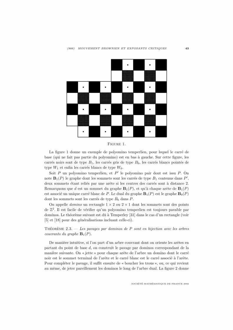
(866) MOUVEMENT BROWNIEN ET EXPOSANTS CRITIQUES 43
Figure 1.
La figure 1 donne un exemple de polyomino temperlien, pour lequel le carre debase (qui ne fait pas partie du polyomino) est en bas a gauche. Sur cette figure, lescarres noirs sont de type B1, les carres gris de type B0, les carres blancs pointes detype W1 et enfin les carres blancs de type W0.
Soit P un polyomino temperlien, et P ′ le polyomino pair dont est issu P . Onnote B1(P ) le graphe dont les sommets sont les carres de type B1 contenus dans P ′,deux sommets etant relies par une arete si les centres des carres sont a distance 2.Remarquons que d est un sommet du graphe B1(P ), et qu’a chaque arete de B1(P )est associe un unique carre blanc de P . Le dual du graphe B1(P ) est le graphe B0(P )dont les sommets sont les carres de type B0 dans P .
On appelle domino un rectangle 1 × 2 ou 2 × 1 dont les sommets sont des pointsde Z2. Il est facile de verifier qu’un polyomino temperlien est toujours pavable pardominos. Le theoreme suivant est du a Temperley [31] dans le cas d’un rectangle (voir[5] et [18] pour des generalisations incluant celle-ci).
Theoreme 2.3. — Les pavages par dominos de P sont en bijection avec les arbrescouvrants du graphe B1(P ).
De maniere intuitive, si l’on part d’un arbre couvrant dont on oriente les aretes enpartant du point de base d, on construit le pavage par dominos correspondant de lamaniere suivante. On « jette » pour chaque arete de l’arbre un domino dont le carrenoir est le sommet terminal de l’arete et le carre blanc est le carre associe a l’arete.Pour completer le pavage, il suffit ensuite de « boucher les trous », ou, ce qui revientau meme, de jeter pareillement les dominos le long de l’arbre dual. La figure 2 donne
SOCIETE MATHEMATIQUE DE FRANCE 2002

44 J.-F. LE GALL
un exemple de pavage par dominos du polyomino de la figure 1 et de l’arbre associedont les sommets sont les points de B1(P ).
Figure 2.
Considerons maintenant, pour un entier pair n, le polyomino temperlien P
rectangulaire defini comme la reunion des carres unite centres aux points de1, 2, . . . , 2n + 1 × −n,−n + 1, . . . , n − 1, n, a l’exception du carre d centre en(1, 0). Soit Q l’ensemble obtenu a partir de P en enlevant un carre noir b adjacenta la frontiere de P (donc de type B1) ainsi qu’un carre blanc w (qu’on peut voircomme une arete de B1(P )).
Lemme 2.4 ([17]). — Les pavages par dominos de Q sont en bijection avec les arbrescouvrants de B1(P ) pour lesquels l’arc de b a d contient l’arete w.
Ce lemme nous permet d’esquisser la methode d’approche du Theoreme 2.1 [17].Nous voulons estimer la probabilite que dans l’arbre couvrant uniforme sur N × Z,l’arc joignant 0 a ∞ contienne l’arete w fixee. Le lemme precedent nous permettrad’estimer la probabilite que pour l’arbre couvrant uniforme dans une boıte rectan-gulaire arbitrairement grande, l’arc joignant le point de base a un autre point de lafrontiere contienne l’arete w. Cette probabilite s’exprimera d’apres le Lemme 2.4 etle Theoreme 2.3 comme le rapport du nombre de pavages par dominos de Q sur lenombre de pavages par dominos de P . Dans les sections suivantes, nous expliquonscomment on estime le nombre de pavages par dominos d’un polyomino temperlien.Ceci ne s’applique pas directement a Q qui n’est pas temperlien, mais la methodepeut etre adaptee.
ASTERISQUE 276
(866) MOUVEMENT BROWNIEN ET EXPOSANTS CRITIQUES 45
2.3. Matrice de Kasteleyn et fonction de couplage
Dans ce paragraphe, nous considerons un polyomino temperlien P et nous notonsM l’ensemble des carres de P . L’ensemble M est muni d’une structure de grapheevidente, ou deux carres sont adjacents ssi ils ont un cote en commun. La matricede Kasteleyn de P est la matrice symetrique K = (K(v, v′), v, v′ ∈ M) telle queK(v, v′) = 0 si v et v′ ne sont pas adjacents et, pour v ∈ M ∩ (W0 ∪W1) et v′ ∈M ,
K(v, v′) =
⎧⎪⎪⎨⎪⎪⎩1 si v′ = v + (1, 0)i si v′ = v + (0, 1)−1 si v′ = v + (−1, 0)−i si v′ = v + (0,−1).
Kasteleyn [14] a montre (avec une definition differente de K) que le nombre depavages par dominos de P est la racine carree du module du determinant de K. Engeneral, sauf dans le cas du rectangle ou une formule explicite existe, il est cependantdifficile d’utiliser ce resultat pour estimer le nombre de pavages par dominos de P .
La fonction de couplage de P est par definition la matrice inverse C = K−1.
Proposition 2.5 ([15]). — Si u, v sont deux carres adjacents de P , la probabilitequ’un pavage aleatoire uniforme de P contienne le domino u, v est egale a |C(u, v)|.
Plus generalement [15], la probabilite qu’un pavage aleatoire uniforme contienneune famille fixee de dominos disjoints s’exprime comme la valeur absolue du determi-nant d’une sous-matrice de C.
Nous verrons dans la partie suivante que si l’on se donne une suite de polyominostemperliens Pε de εZ2 qui approchent une region du plan, il est possible d’obtenir desinformations precises sur le comportement asymptotique des fonctions de couplage Cε
associees. Afin de mieux comprendre l’origine de ces informations, donnons quelquesproprietes simples de la fonction de couplage.
Si on enumere les elements de M en ecrivant successivement les carres de type W0,W1, B0 et enfin B1, la matrice K est de la forme
K =
⎛⎜⎜⎝0 0 K1 iK2
0 0 iK3 K4
Kt1 iKt
3 0 0iKt
2 Kt4 0 0
⎞⎟⎟⎠ou les matrices K1, K2, K3, K4 sont reelles. Il est facile de voir que l’inverse de K doitetre aussi de cette forme. En particulier, C(v, v′) = 0 si v et v′ sont tous les deuxblancs, ou tous les deux noirs, C(v, v′) est reel quand v′ = v + (1, 0) modulo 2 etimaginaire pur quand v′ = v + (0, 1) modulo 2.
Par definition de C, on a KC(v, v′) = δv(v′), ou δv est la fonction indicatrice dusingleton v. Notons K∗ la matrice conjuguee de K. On verifie facilement que la
SOCIETE MATHEMATIQUE DE FRANCE 2002

46 J.-F. LE GALL
matrice K∗K agit sur les fonctions definies sur B0(P ), et que pour une telle fonctionf on a pour tout v ∈ B0(P ),
(2) K∗Kf(v) = 4f(v)− f(v+(2, 0))− f(v+(−2, 0))− f(v+(0, 2))− f(v+(0,−2)).
Cette formule est vraie meme si les quatre voisins (dans B0) de v ne sont pas tousdans B0(P ), auquel cas il faut affecter la valeur 0 a la fonction f aux points exterieursa B0(P ). La formule precedente s’interprete en disant que K∗K = ∆ est (4 fois) leLaplacien discret sur B0(P ), avec conditions de Dirichlet au bord. Ce qui precedereste vrai si on remplace B0(P ) par B1(P ) = B1(P )\d, mais la formule (2) doitetre modifiee si v est adjacent a la frontiere de P . Dans ce cas, le terme de droite de(2) est f(v) multiplie par le nombre de voisins de v dans B1(P ) moins la somme desvaleurs de f en ces voisins (en prenant f(d) = 0).
En appliquant K∗ a l’egalite KC(v, v′) = δv(v′), on trouve pour v ∈W0 ∪W1,
∆C(v, ·) = δv+(1,0) − δv+(−1,0) − iδv+(0,1) + iδv+(0,−1).
Fixons v ∈ W0 ∩ M . La restriction, notee f , de C(v, ·) a B0(P ) est a valeursreelles, et l’egalite precedente montre que cette fonction est harmonique (au sensdiscret) sur B0(P )\v− (1, 0), v + (1, 0), avec conditions frontiere de type Dirichlet.En revanche la restriction, notee ig, de C(v, ·) a B1(P ) est a valeurs imaginaires pureset est harmonique sur B1(P )\v + (0, 1), v + (0,−1). Les conditions frontiere sontmaintenant de type Neumann : la valeur de g en un point frontiere v′ est la moyennede ses valeurs aux voisins de v′ dans B1(P ), en prenant g(d) = 0.
De plus, on peut dire que g est la conjuguee harmonique de f , au sens ou on a lesequations de Cauchy-Riemann discretes
∂xf(v′) = ∂yg(v′) pour v′ ∈ (M ∩W0)\v∂yf(v′) = −∂xg(v′) pour v′ ∈M ∩W1,
avec la notation ∂xf(v) = f(v+(1, 0))−f(v+(−1, 0)), ∂yf(v) = f(v+(0, 1))−f(v+(0,−1)).
On a des resultats analogues pour la fonction C(v, ·) lorsque v ∈ W1.
2.4. Comportement asymptotique de la fonction de couplage
Soit U un polygone rectiligne de R2 (U est un domaine simplement connexe et safrontiere est composee de segments paralleles aux axes), et soit d0 ∈ ∂U . Consideronspour chaque ε > 0 un polyomino temperlien Pε de εZ2, et supposons que ces poly-ominos convergent vers U de la maniere evidente (en particulier, Pε a autant de coinsque U , et chaque coin de Pε converge vers le coin correspondant de U). On supposeaussi que les points de base dε de Pε convergent vers le point d0.
Notons Cε la fonction de couplage de Pε et Mε l’ensemble des carres de Pε.
ASTERISQUE 276

(866) MOUVEMENT BROWNIEN ET EXPOSANTS CRITIQUES 47
Theoreme 2.6 ([16]). — Soient, pour chaque ε > 0, uε, vε, wε, xε des elements deMε appartenant respectivement a W0, W1, B0, B1, et convergeant respectivement versdes points distincts u, v, w, x ∈ U . Alors,
limε→0
1εCε(uε, wε) = ReF0(u, w)
limε→0
1εCε(uε, xε) = i ImF0(u, x)
limε→0
1εCε(vε, wε) = Re F1(v, w)
limε→0
1εCε(vε, xε) = i Im F1(v, x)
ou les fonctions F0 et F1 sont caracterisees par les proprietes suivantes.Pour v ∈ U , la fonction F0(v, ·) est meromorphe sur U , sa partie reelle s’annule
sur ∂U , elle a un zero en z = d0, un pole simple de residu 1π en z = v et pas d’autre
pole sur U .De meme, la fonction F1(v, ·) est meromorphe sur U , sa partie imaginaire s’annule
sur ∂U , elle a un zero en z = d0, un pole simple de residu 1π en z = v et pas d’autre
pole sur U .
Remarque — Un resultat analogue est vrai pour des ouverts U plus generaux : voir[16].
Les proprietes des fonctions F0 et F1, et le fait qu’on obtienne tantot ReF tantotIm F , viennent directement des proprietes des fonctions de couplage decrites dansla partie precedente. Donnons rapidement l’idee de la preuve du theoreme. On noteB′
0(Pε) le graphe obtenu en ajoutant a B0(Pε) tous les carres noirs (de type B0) quisont adjacents a un carre blanc a la frontiere de Pε, et les aretes reliant deux carresnoirs si le carre blanc situe entre eux est dans Pε. Soit alors Gε(w, w′) la fonction deGreen de B′
0(Pε) : pour w ∈ B0(Pε), la fonction Gε(w, ·) verifie ∆Gε(w, ·) = δw surB0(Pε), et Gε(w, w′) = 0 pour w′ ∈ B′
0(Pε)\B0(Pε). Par abus de notation, ecrivonsRe Cε(uε, ·) pour la restriction de Cε(uε, ·) a B0(Pε) (qui est a valeurs reelles) etprolongeons-la a B′
0(Pε) en lui donnant la valeur 0 sur B′0(Pε)\B0(Pε). Nous avons
vu que, sur B0(Pε),∆Re Cε(uε, ·) = δuε+ε − δuε−ε.
Puisque Re Cε(uε, ·) s’annule a la frontiere, il en decoule que
Re Cε(uε, w) = Gε(uε + ε, w)−Gε(uε − ε, w).
On peut alors deduire la premiere convergence du theoreme de resultats sur le com-portement asymptotique des fonctions de Green discretes.
Les fonctions de couplage asymptotiques F0 et F1 possedent des proprietes d’inva-riance conforme qui sont tres importantes pour les applications. Posons FU
+ = F0 +F1
SOCIETE MATHEMATIQUE DE FRANCE 2002

48 J.-F. LE GALL
et FU− = F0 − F1. Alors, FU
+ (v, z) est meromorphe en v et en z, et FU− (v, z) est me-
romorphe en z et anti-meromorphe en v. De plus, si f : V −→ U est une bijectionconforme envoyant le point de base de V sur le point de base de U , on a :
FV+ (v, z) = f ′(v)FU
+ (f(v), f(z)),
FV− (v, z) = f ′(v)FU
− (f(v), f(z)).
2.5. L’asymptotique du nombre de pavages par dominos
Dans ce paragraphe, nous decrivons brievement un resultat important de [17] don-nant l’asymptotique du logarithme du nombre N(Pε) de pavages par dominos dePε (sous les hypotheses de la partie precedente). Ce resultat ne peut pas etre ap-plique directement a la preuve du Theoreme 2.1, qui necessite d’estimer le rapportN(Qε)/N(Pε) ou Qε n’est pas temperlien. Cependant, les techniques impliquees danscette preuve sont proches de celles que nous decrivons tres succinctement ci-dessous.
Nous notons Aε l’aire de Pε, perim(Pε) son perimetre, et V le nombre de sommetsdu polygone V .
Theoreme 2.7 ([17]). — Soit N(Pε) le nombre de pavages par dominos de Pε. Alors,
log N(Pε) =c0Aε
ε2+
c1 perim(Pε)ε
− 12
log1ε− V − 4
36h(ε) + c2(U) + o(1),
ou c0 = Gπ , si G = 1− 1
32 + 152 − . . . est la constante de Catalan, c1 = G
2π + log(√
2−1)4 ,
c2(U) est une constante dependant seulement de U , et la fonction h est independantede U et verifie h(ε) = log 1
ε + o(log 1ε ).
Remarque. — Le premier terme du developpement ci-dessus est essentiellementcontenu dans le travail de Burton et Pemantle [5].
Dans le cas particulier ou U est un rectangle, le developpement du theoreme peutetre obtenu a partir des expressions explicites dues a Kasteleyn [13] et Temperleyet Fischer [32] (voir [10] pour une derivation du developpement dans ce cas). Pourse ramener au cas du rectangle, on utilise une technique de decoupage. Consideronsun segment (vertical ou horizontal) γ′ qui traverse U , touche ∂U seulement en sespoints de depart et d’arrivee, et evite le point de base d0 de U . Pour chaque ε > 0,considerons aussi une bande γε de largeur ε formee de carres de Pε, qui traverse Pε enrestant a une distance O(ε) de γ′. On peut imposer que les carres noirs contenus dansγε soient de type B0, et que si l’une ou l’autre extremite de γ′ est a un coin concavede U , l’extremite correspondante de γε soit au coin correspondant de Pε.
La longueur de γε doit alors etre un multiple impair de ε. Si nous retirons la bandeγε de Pε, il reste deux polyominos disjoints. Celui, note P1, qui contient le carre debase de Pε est temperlien. L’autre, note P2, devient temperlien si on lui enleve unseul carre s de type B1 adjacent a l’un des points terminaux de γε. Remarquons que
ASTERISQUE 276
(866) MOUVEMENT BROWNIEN ET EXPOSANTS CRITIQUES 49
la reunion γε ∪ s a un seul pavage par dominos. Le nombre de pavages par dominosde Pε est egal au produit du nombre de pavages de P1 et du nombre de pavages deP2, divise par la probabilite que le pavage de γε ∪ s apparaisse dans un pavage de Pε
tire au hasard uniformement.
Nous pouvons repeter cette procedure a partir de P1 et P2 de maniere a decouperle polyomino initial en des morceaux de plus en plus simples. Au bout d’un nombrefini d’iterations on arrive a des rectangles temperliens pour lesquels on peut utiliserla formule exacte. Tout le probleme est donc d’estimer la probabilite que dans unpavage aleatoire uniforme de Pε, apparaisse le pavage de γε ∪ s. Notons a1, . . . , aN lesdominos qui forment ce pavage. Les ai sont mis bout a bout (a partir de la frontiere)sauf pour aN qui est perpendiculaire aux autres. La probabilite que tous les ai soientpresents s’ecrit comme le produit
N∏j=1
P (aj | a1, . . . , aj−1)
des probabilites conditionnelles que aj soit present sachant que a1, . . . , aj−1 le sont.Pour j fixe, cette derniere probabilite conditionnelle est la probabilite que aj soitpresent dans un pavage aleatoire de la region P
(j)ε := Pε\a1, . . . , aj−1, qui est elle-
meme un polyomino temperlien. Soit C(j)ε la fonction de couplage de P
(j)ε , et soient
u(j)ε , v
(j)ε les deux carres qui composent le domino aj . Alors, la probabilite que aj
soit present dans un pavage aleatoire de P(j)ε est d’apres la Proposition 2.5 egale a
|C(j)ε (u(j)
ε , v(j)ε )|. Le comportement asymptotique de ces quantites peut etre decrit en
termes des fonctions de couplage asymptotiques F0, F1 de la partie 4, correspondanta la region U privee d’une coupure le long (d’une partie) du segment γ′. A l’aided’une analyse detaillee de ces asymptotiques et d’une utilisation intensive des pro-prietes d’invariance conforme, cela conduit a des estimations suffisamment precisespour etablir le Theoreme 2.7.
REFERENCES
[1] L. V. Ahlfors – Conformal Invariants, Topics in Geometric Function Theory.McGraw-Hill, New York 1973
[2] K. Burdzy, G. F. Lawler – Non-intersection exponents for random walk andBrownian motion. Part I : Existence and an invariance principle. Probab. Th.Rel. Fields 84 (1990), 393-410.
[3] K. Burdzy, G. F. Lawler – Non-intersection exponents for random walk andBrownian motion. Part II : Estimates and applications to a random fractal. Ann.Probab. 18 (1990), 981-1009.
SOCIETE MATHEMATIQUE DE FRANCE 2002

50 J.-F. LE GALL
[4] K. Burdzy, W. Werner – No triple point of planar Brownian motion is ac-cessible. Ann. Probab. 24 (1996), 125-147.
[5] R. Burton, R. Pemantle – Local characteristics, entropy and limit theoremsfor spanning trees and domino tilings via transfer impedances. Ann. Probab. 21(1993), 1329-1371.
[6] M. Cranston, T. Mountford – An extension of a result by Burdzy and Law-ler. Probab. Th. Rel. Fields 89 (1991), 487-502.
[7] B. Duplantier – Loop-erased self-avoiding walks in two dimensions : exactcritical exponents and winding numbers. Physica A 191 (1992), 516-522.
[8] B. Duplantier – Random walks and quantum gravity in two dimensions. Phys.Rev. Lett. 81 (1998), 5489-5492.
[9] B. Duplantier – Two-dimensional copolymers and exact conformal multifrac-tality. Phys. Rev. Lett. 82 (1999), 880-883.
[10] B. Duplantier, F. David – Exact partition functions and correlation functionsof multiple Hamiltonian walks on the Manhattan lattice. J. Stat. Phys. 51 (1988),327-434.
[11] B. Duplantier, K.-H. Kwon – Conformal invariance and intersections ofrandom walks. Phys. Rev. Lett. 61 (1988), 2514-2517.
[12] B. Duplantier, G. F. Lawler, J. F. Le Gall, T. J. Lyons – The geometryof the Brownian curve. Bull. Sci. math. 117 (1993), 91-106.
[13] P. Kasteleyn – The statistics of dimers on a lattice. I. The number of dimerarrangements on a quadratic lattice. Physica 27 (1961), 1209-1225.
[14] P. Kasteleyn – Graph theory and crystal physics. In : Graph Theory and Theo-retical Physics. Academic Press, London 1967
[15] R. Kenyon – Local statistics of lattice dimers. Ann. Inst. Henri Poincare Probab.Stat. 33 (1997), 591-618.
[16] R. Kenyon – Conformal invariance of domino tilings. Preprint.[17] R. Kenyon – The asymptotic determinant of the discrete Laplacian. Preprint.[18] R. Kenyon, J. Propp, D. Wilson – Trees and matchings. Preprint.[19] G. F. Lawler – A self-avoiding random walk. Duke Math. J. 47 (1980), 655-693.[20] G. F. Lawler – Intersections of Random Walks. Birkhauser, Boston 1991[21] G. F. Lawler – Hausdorff dimension of cut points for Brownian motion. Elec-
tron. J. Probab. 1 (1996), no 2.[22] G. F. Lawler – The dimension of the frontier of planar Brownian motion.
Electronic Commm. Probab. 1 (1996), no 5.[23] G. F. Lawler – Loop-erased random walk. In : Perplexing Problems in Proba-
bility. Birkhauser, Boston 1999[24] G. F. Lawler, W. Werner – Intersection exponents for planar Brownian
motion. Preprint.
ASTERISQUE 276

(866) MOUVEMENT BROWNIEN ET EXPOSANTS CRITIQUES 51
[25] G. F. Lawler, W. Werner – Universality for conformally invariant intersec-tion exponents. Preprint.
[26] G. F. Lawler, O. Schramm, W. Werner – Values of Brownian intersectionexponents I : Half-plane exponents. Preprint.
[27] S. N. Majumdar – Exact fractal dimension of the loop-erased self-avoiding walkin two dimensions. Phys. Rev. Lett. 68 (1992), 2329-2331.
[28] B. B. Mandelbrot – The Fractal Geometry of Nature. Freeman 1982.[29] R. Pemantle – Choosing a spanning tree for the integer lattice uniformly. Ann.
Probab. 19 (1991), 1559-1574.[30] O. Schramm – Scaling limits of loop-erased random walks and uniform spanning
trees. Preprint.[31] H. Temperley – Combinatorics : Proceedings of the British Combinatorial
Conference 1973. London Math. Soc. Lecture Notes Series 13 (1974), 202-204.[32] H. Temperley, M. Fisher – The dimer problem in statistical mechanics – an
exact result. Phil. Mag. 6 (1961), 1061-1063.[33] W. Werner – Asymptotic behaviour of disconnection and intersection expo-
nents. Probab. Th. Rel. Fields 108 (1997), 131-152.
Jean-Francois LE GALL
DMA – Ecole normale superieure45, rue d’UlmF-75230 PARIS Cedex 05E-mail : [email protected]
SOCIETE MATHEMATIQUE DE FRANCE 2002


Seminaire BOURBAKI Novembre 199952e annee, 1999-2000, no 867, p. 53 a 72
LA CORRESPONDANCE DE McKAY
by Miles REID
1. COMMENT C’EST
1.1. Model case: the binary dihedral group BD4n
For G ⊂ SL(2, C) a finite group, the quotient variety X = C2/G is called a Kleinquotient singularity. I draw the quotient map π : C2 → X and the minimal resolutionof singularities Y → X together in the diagram:
C2π
Yϕ−→ X
This situation has been well studied, since Klein around 1870 and Coxeter and Du Valin the 1930s: the subgroup G is classified as cyclic, binary dihedral or a binary groupcorresponding to one of the Platonic solids; the quotient singularity is a hypersurfaceX ⊂ C3 with defining equation one of a list of simple functions. The resolution Y isa surface with KY = ϕ∗KX , and the exceptional locus ϕ−1(0) ⊂ Y of the resolutionconsists of a bunch of −2-curves Ei (that is, Ei
∼= P1C and Ei has self-intersection
E2i = −2), and the intersection EiEj is given by one of the Dynkin diagrams An, Dn,
E6, E7, E8. To avoid writing out lists, let us simply discuss the binary dihedral group
G = BD4n = 〈α, β〉 , where α =(
ε 00 ε−1
), β =
(0 1−1 0
)where ε = exp 2πi
2n . If u, v are coordinates on C2, the G-invariant polynomials are
C[x, y, z]/(z2 − yx2 + 4yn+1), where x = u2n + v2n, y = u2v2, z = uv(u2n − v2n);
thus the quotient variety is the singularity X : (z2 = yx2 − 4yn+1) ⊂ C3 of typeDn+2, and the quotient morphism π : (u, v) → (x, y, z). The resolution of singularities
SOCIETE MATHEMATIQUE DE FRANCE 2002

54 M. REID
Y → X has exceptional locus consisting of −2-curves E1, . . . , En+2 forming the Dn+2
configuration:
(1.1) E1
E2
· · ·
En−1
En+1
En+2
The classical McKay correspondence begins in the late 1970s with the observationthat the same graph arises in connection with the representation theory of G. For agroup G and a given representation Q, the McKay graph (or McKay quiver) has anode for each irreducible representation, and an edge V → V ′ whenever V ′ is a directsummand of V ⊗Q. In our case, BD4n has the 2-dimensional representations
Vi∼= C2, with action α =
(εi 00 ε−i
), β =
(0 1
(−1)i 0
)for i = 0, . . . , n.
This is irreducible for 0 < i < n, and splits into 2 eigenlines when i = 0 or n. Theinclusion G ⊂ SL(2, C) provides the given representation Q = V1. It is a simpleexercise [Homework] to write down the action of G on a basis ei ⊗ e′j of Q⊗ Vi toget Vi ⊗ Q = Vi−1 ⊕ Vi+1 for 0 < i < n, so that the McKay graph of BD4n is theextended Dynkin diagram Dn+2:
(1.2) Dn+2
1 ©
©
© © . . . ©
©
©
V1 V2 Vn−1
Here 1 is the trivial 1-dimensional representation.This example, and the other SL(2, C) cases observed by McKay, suggest that there
is a one-to-one correspondence between the components of the exceptional locus ofY → X in (1.1) and the nontrivial irreducible representations of G ⊂ SL(2, C) in(1.2). This talk explains this coincidence in several different ways, and discusseshigher dimensional generalisations.
1.2. General assumption
I use the following diagram throughout:
(1.3)
Mπ
Yϕ−→ X = M/G
ASTERISQUE 276
(867) LA CORRESPONDANCE DE McKAY 55
Here M is a quasiprojective algebraic manifold with KM = 0 and G a finite auto-morphism group of M that acts trivially on a global basis sM ∈ H0(KM ). The objectof study is the quotient variety X = M/G and its resolutions Y → X , sometimesassumed to have KY = 0. An important motivating case is a finite subgroup G ⊂SL(3, C) acting on M = C3.
1.3. Definition–Reassurance
The quotient varieties X = M/G occuring here are singular. The theory of minimalmodels of higher dimensional algebraic varieties (Mori theory) has a whole batteryof definitions that deal systematically with singular varieties; here I only need onesmall item: the orbifolds X here have trivial canonical class KX = 0 (or trivial Serre–Grothendieck dualising sheaf ωX = OX). In concrete terms, this means the following:X is a complex n-fold (algebraic or analytic variety), nonsingular in codimension 1,and its nonsingular locus NonSing X has an everywhere nondegenerate holomorphic n-form sX (deduced from sM ). So sX is a complex volume element at every nonsingularpoint of X , or in other words, it is a global basis of Ωn
NonSing X . A resolution ofsingularities ϕ : Y → X is crepant if KY = ϕ∗KX or ωY = ϕ∗ωX , which simplymeans that Y is a nonsingular n-fold with KY = 0 or ωY = Ωn
Y = OY · sY , wheresY = ϕ∗sX . More generally, an arbitrary proper birational map ϕ : V → X has adiscrepancy divisor ∆ϕ =
∑aiEi defined by KV = ϕ∗KX +
∑aiEi with ai ≥ 0; a
divisor Ei is crepant if ai = 0. The discrepancy ∆ϕ is the divisor of zeros on V of thebasic n-form sX on X , generalising the divisor of zeros of the Jacobian determinant;in Mori theory, it measures how far V is from minimal.
1.4. Summary and slogan
I start with a preview of different approaches to the McKay correspondence, whichare treated in more detail in later sections. Each of these approaches gives a result inthe case of a finite subgroup G ⊂ SL(3, C) acting on M = C3.
(1) Gonzalez-Sprinberg and Verdier sheaves: the first direct link from the repre-sentation theory of G to the geometry of the resolution Y → X was the work ofGonzalez-Sprinberg and Verdier [GSpV]: for a Kleinian subgroup G ⊂ SL(2, C), theyconstructed sheaves Fρ on Y , indexed by the irreducible representations of G, whosefirst Chern classes base the cohomology of Y .
(2) String theory: the first hint of a McKay correspondence in higher dimensionscomes from work of the string theorists Dixon, Harvey, Vafa and Witten [DHVW]around 1985: if G ⊂ SL(3, C) and Y → X = C3/G is a crepant resolution of thequotient C3/G, the Euler number of Y equals the number of conjugacy classes of G
(or the number of its irreducible representations).(3) Explicit methods: the finite subgroups G ⊂ SL(3, C) are classified, and work
in the early 1990s of Roan, Ito, Markushevich and others proved case-by-case the
SOCIETE MATHEMATIQUE DE FRANCE 2002

56 M. REID
existence of crepant resolutions, and the validity of the formula of [DHVW] for theBetti numbers of Y .
(4) Valuation theory: for a finite subgroup G ⊂ SL(n, C), the paper [IR] shows thatG has a grading by age, analogous to the weight grading in Hodge theory, and provesthat the conjugacy classes of junior elements g ∈ G (elements of age 1) correspondone-to-one with the crepant divisors of a resolution (more precisely, their discretevaluations). This result holds for any G ⊂ SL(n, C) and is intrinsic, classification-free; but for n ≥ 4 it only gives a small part of a McKay correspondence (so far).
(5) Nakamura’s G-Hilbert scheme: a resolution of singularities Y → X , even ifit is a Mori minimal model theory, is not at all unique. Moreover, if X = M/G,the construction of a resolution Y need not have much to do with G. In 1995,Nakamura made the revolutionary suggestion that in many interesting cases, the G-Hilbert scheme is a preferred resolution Y of X (see [IN2], [N], [R]). When this holds,Y is a “very good” moduli space over M , and the general yoga of moduli suggeststhat there should be a “tautological” treatment of the geometry of Y (comparable tothe cohomology of Grassmann varieties).
(6) Fourier–Mukai transform: the derived category D(V ) of coherent sheaves on avariety V (considered up to isomorphism of triangulated categories) can be used as ageometric characteristic of V , in place of K theory or cohomology. The Fourier–Mukaitransform is a general method for constructing isomorphisms of derived categories (see[Mu], [O], [BO1], [Br], [BrM]). Bridgeland and others [BKR] have recently used thistechnique to prove that, if Y = G-Hilb M is a crepant resolution, then DG(M) =D(Y ). This implies the corresponding result in K theory.
(7) Motivic integration: the motivic integration of Batyrev, Denef and Loeser, andKontsevich is a rigorous and comparatively simple mathematical trick that mimicssome aspects of the path integrals of QFT. Very roughly, if ϕ : Y → X is a resolutionof singularities, possibly far from minimal, with discrepancy divisor KY − ϕ∗KX =∑
aiEi, the calculation amounts to defining the stringy homology of X by pickingonly 1
ai+1 th of the homology of Ei. Quite remarkably, this is well defined, agrees withthe predictions of [DHVW] mentioned in (2) above, and provides an exact form of thehomological McKay correspondence for finite subgroups G ⊂ SL(n, C).
(8) Explicit methods (bis): for a finite group G ⊂ SL(3, C), the results of (6)(maybe also (7)) imply that Gonzalez-Sprinberg–Verdier sheaves Fρ base the K theoryof the resolution Y → X , so that their Chern classes or Chern characters base thecohomology. Reworking this in explicit terms presents a treasure chest of delightfulcomputational problems – already the Abelian cases lead to lovely pictures (compare[R], [CR], [C2]).
I believe that many other approaches to the McKay correspondence remain to bediscovered, and many interrelations between the different approaches; this problemarea is recommended to afficionados of noncommutative geometry, perverse sheaves,
ASTERISQUE 276

(867) LA CORRESPONDANCE DE McKAY 57
Gromov–Witten invariants, elliptic cohomology, Chow groups, etc. Here is an attemptto describe the subject in a single statement:
Principle 1.1. — Let M be an algebraic manifold, G a group of automorphisms ofM , and Y → X a resolution of singularities of X. Then the answer to any well posedquestion about the geometry of Y is the G-equivariant geometry of M .
I give two illustrationsI. If G ⊂ SL(n, C) acts on Cn and the quotient X = Cn/G has a crepant resolution
Y → X , the homology or K theory of Y is expected (or known) to be independentof Y . In this case, the principle says that the homology or K theory of Y is therepresentation theory of G (equal to the G-equivariant geometry of Cn because Cn iscontractible).
II. Let M be a Calabi–Yau n-fold and G a group of automorphisms of M thatacts trivially on Ωn
M . The stringy homology of X = M/G (see Sections 3 and 4) iswell defined by [DL1]. The principle says that it must agree with the G-equivarianthomology of M . (I expand on what this means in Section 4.)
Viewed as an orbifold or stack, X = M/G contains M and the G action, and youcan of course derive tautological question-and-answer pairs from this (this is oftenpopular as a source of questions after the talk). The content of my slogan is thatthe equivariant geometry of M already knows about the crepant resolution Y → X .Minimal models exist for surfaces by classical work, and for 3-folds by Mori theory (orby explicit methods). Minimal models of orbifolds by finite subgroups G ⊂ SL(3, C)provide infinitely many examples of local models of Calabi–Yau 3-folds; calculatingtheir Betti numbers or K theory in a priori terms is in no sense a tautology. Ifyou prefer to think of the singular X as the fundamental object, and not resolve it(a perfectly sensible alternative), the content is that X has invariants that can bedescribed from the orbifold M/G, but are birationally invariant under appropriateconventions about resolutions.
2. AGE AND DISCREPANCY
Let G ⊂ SL(n, C) be a finite group; any element g ∈ G has finite order r, say. Forany such r, I choose at the outset a primitive rth root of 1, say exp 2πi
r . A choice ofeigenbasis diagonalises the action of g ∈ G on M = Cn, giving
(2.1) g = diag(εa1 , . . . , εan) with 0 ≤ ai < r.
I write g = 1r (a1, . . . , an), possibly depending on the choices made. Now
∑ai ≡ 0
mod r because g ∈ SL(n, C). Following [IR], define the age of g by age g = 1r
∑ai.
As we will see, this is an analog of weight in Hodge theory; Denef and Loeser [DL2]refer to it by the long-winded but not inappropriate term valuation theoretic weight .
SOCIETE MATHEMATIQUE DE FRANCE 2002

58 M. REID
Clearly, age g is an integer in the range [0, . . . , n− 1], and only the identity has age 0.The elements of age 1 are junior.
Junior elements of G give rise to crepant divisors of a resolution V → M/G bythe following toric mechanism (for more details, and a picture, see [IR], 2.6–7). Forg ∈ G (not the identity), consider the ai of (2.1), and suppose (a1, . . . , an) ∈ Zn isprimitive. The coordinate subspace corresponding to the xi with ai = 0 is the fixedlocus Fix g; it splits off as a direct product, and I assume that all ai > 0 to short-cutsome simple arguments. A useful example to bear in mind is when all the ai = 1(compare Example 4.1).
I view the integers (a1, . . . , an) as weights. They define the grading wtxi = ai
on the coordinate ring C[x1, . . . , xn], or equivalently, the action xi → λaixi of C∗ onM = Cn that defines the weighted projective space
P(a1, . . . , an) = (Cn \ 0)/C∗.
We obtain the weighted blowup Bg → M as the closed graph of the quotient mapM P(a1, . . . , an); it has the exceptional divisor Bg ⊃ Eg = P(a1, . . . , an). Obvi-ously g acts on Bg, and fixes Eg pointwise (because g acts on M as ε ∈ C∗). ThereforeBg → Bg/ 〈g〉 is totally ramified along Eg.
Theorem 2.1 ([IR], 2.6–7). — Suppose that V → X is any resolution of singulari-ties of the quotient X = M/G. Then V contains a divisor Fg rationally dominatedby Eg under the rational map Bg → M V . The discrepancy of Fg is given byaFg = age g − 1, and in particular
Fg is crepant ⇐⇒ g is junior.
Every crepant divisor of any resolution V occurs thus.
Discussion of proof. — Write Xg = M/ 〈g〉 for the partial quotient. ThenBg/ 〈g〉 → Xg is a partial resolution, with the single exceptional divisor Eg. An easytoric calculation gives the discrepancy of Eg ⊂ Bg or Eg ⊂ Bg/ 〈g〉 (compare [YPG],4.8): the standard basis of Ωn
M is sM = dx1 ∧ · · · ∧ dxn. For KBg , choose a Laurentmonomial y1 = xm of weight 1 (recall that the ai were coprime). Then y1 is thedefining equation of Eg ⊂ Bg at a general point of Eg (away from all the coordinatehyperplanes), and yr
1 that of Eg ⊂ Bg/ 〈g〉. Choosing Laurent monomials y2, . . . , yn
forming a basis of the lattice of monomials of weight 0, we get that
sBg = dy1 ∧ · · · ∧ dyn ∈ ΩnBg
is the required basis. The discrepancy is the exponent a in sM = (unit) · ya1sBg ,
and is determined by weighty considerations: sM has weight∑
ai and sBg weight1, so a =
∑ai − 1. On the quotient Bg/ 〈g〉 we only have yr
1, so we get the stateddiscrepancy 1
r
(∑ai − 1− (r − 1)
)= age g − 1.
ASTERISQUE 276
(867) LA CORRESPONDANCE DE McKAY 59
The quotient morphism M → X is a Galois cover with group G; a cyclic subgroup〈g〉 corresponds to an intermediate cover M →M/ 〈g〉 = Xg → X . The reduction toa cyclic group is in terms of ramification theory; see [IR], 2.6–7. Roughly, over thegeneral point of any exceptional divisor F of V → X , the Galois extension of functionfields k(X) ⊂ k(M) forms a tower, starting with a cyclic ramified cover. For a crepantexceptional divisor, the cyclic ramification can be chased back up to a conjugacy classof junior elements g ∈ G.
Remark 2.2. — This argument works in all dimensions, but it only identifies the divi-sors of a crepant resolution Y , and thus only gives a basis of H2(Y, Q) or H2n−2(Y, Z)corresponding in McKay style to junior conjugacy classes of G. In 3 dimensions, weused Poincare duality to bootstrap ourselves up to a basis of H∗(Y, Q) in [IR]. His-torically, this was the first intrinsic proof of the conjectured formula of [DHVW] forthe Betti numbers of a crepant resolution.
As Brylinski [B] remarks (following Mumford), if V → X is any resolution, thegroup G can be viewed as the fundamental group of V minus the branch locus, sothat an exceptional divisor F of a resolution V corresponds directly to a conjugacyclass of G as a little anticlockwise loop around F ; for crepant divisors, this is of coursethe same relation as in [IR]. But I don’t know how to use this idea to get a well definedrelation between, say, codimension 2 cycles of Y and age 2 conjugacy classes of G.
3. L’INNOMMABLE
This section is mainly for sociological and historical interest, but some harmless hi-larity may derive from my garrulous display of incompetence and ignorance in physics.
A theoretical prediction of string theory: Fermionic strings propagate in 10-dimensional space-time. Indeed, a universe of any other dimension would haveparticles moving faster than the speed of light. Since this prediction, on the face of it,contradicts the empirically observed 4-dimensions of space-time, string theorists want6 of the dimensions to be filled up with tiny Calabi–Yau 3-folds. (This means (i) a6-dimensional Riemannian manifold with SU(3) holonomy, or (ii) a complex manifoldV with a Ricci flat Kahler metric and H1(V, R) = 0, or (iii) an algebraic manifold V
with KV = 0 and H1(V,OV ) = 0. It seems that the holonomy or Kahler conditionson V , together with some finite volume, are required by the physics, whereas makingV nonsingular, compact, and a constant fibre over macroscopic space-time are justconvenient choices when you try to guess a model.)
The two papers [DHVW] were concerned with trying to calculate string theory onexamples of Calabi–Yau varieties obtained by dividing a 3-dimensional complex torusM by a finite group G preserving a basic holomorphic 3-form, so that the stabilisersubgroup at any point is a subgroup of SL(3, C). A closed string on the quotient may
SOCIETE MATHEMATIQUE DE FRANCE 2002

60 M. REID
lift either to a closed string on the cover, or to a path that goes from x to g · x. Thelatter are called twisted sectors. The physicists need to take care of these in orderto relate
∫X
to G-equivariant∫
M, and they are the key to the form of the McKay
correspondence in Theorem 4.4, (4).Taking limits is a tradition in physics, where the old is frequently the limit of
the new: Newtonian mechanics is the limit of special relativity as c → ∞, classicalmechanics the limit of quantum physics as → 0, groups and their Hopf algebras thelimit of quantum groups as q → 1. In string theory, if the scale (or radius of curvature)of the tiny Calabi–Yau tends to zero, the theory should approximate ordinary Lorentz4-dimensional space-time, whereas letting it tend to macroscopic proportions wouldapproximate flat Lorentz 10-dimensional space-time. In this context, the twistedsector near a point x ∈ MH plays the role of strings that are topologically nontrivial,but are allowed to remain of finite length (and so contribute to path integrals) asthe scale becomes large. To calculate something called the 1-loop partition function,DHVW considered mapping the elliptic curve S1 × S1 (with parameters σ and τ
along the copies of S1) into X , or the σ, τ square into M with equivariant boundaryconditions depending on g, h. Thinking about twisted sectors and limits led DHVW(I confess that their logic eludes me somewhat) to the formula
(3.1) estring(X) = e(M, G) :=1|G|
∑g,h∈G
commuting
e(M 〈g,h〉).
Here e(M, G) on the left-hand side is the G-equivariant Euler number of M ; on theright-hand side, the sum runs over all commuting pairs of elements of G, 〈g, h〉 isthe Abelian group they generate, M 〈g,h〉 its fixed locus in M , and e is the usualEuler number. The formula is a replacement for the Euler number of the singularorbifold X . The papers [DHVW] contain more-or-less explicitly the conjecture thatthis number is the Euler number of a minimal resolution of singularities.
It is not hard (see [HH], [Roan] and [Homework]) to rearrange the sums in (3.1) togive
(3.2) estring(X) = e(M, G) =∑
[H]⊂G
e(XH)× card[h] ∈ H,
where (i) the first sum runs over conjugacy classes of subgroups H ⊂ G; (ii) thestratum XH is the set of x ∈ X such that Stab y is conjugate to H for any pointy ∈ M over x; (iii) the second factor is the number of conjugacy classes in H . Thismeans that XH ⊂ X contributes to e(M, G) with multiplicity the representationtheory of H .
Remark 3.1. — The physicists want to do path integrals, that is, they want to inte-grate some “Action Man functional” over the space of all paths or loops γ : [0, 1]→ Y .This impossibly large integral is one of the major schisms between math and fizz.
ASTERISQUE 276

(867) LA CORRESPONDANCE DE McKAY 61
The physicists learn a number of computations in finite terms that approximate theirpath integrals, and when sufficiently skilled and imaginative, can use these to derivemarvellous consequences; whereas the mathematicians give up on making sense ofthe space of paths, and not infrequently derive satisfaction or a misplaced sense ofsuperiority from pointing out that the physicists’ calculations can equally well be used(or abused!) to prove 0 = 1. Maybe it’s time some of us also evolved some skill andimagination. The motivic integration treated in the next section builds a miniaturemodel of the physicists’ path integral, by restricting first to germs of holomorphicpaths γ : U → Y , where 0 ∈ U ⊂ C is a neighbourhood of 0, then to formal powerseries γ : Spec C[[z]]→ Y .
4. MOTIVIC INTEGRATION
The material in this section is due to Batyrev [Ba1], [Ba2], Denef and Loeser [DL1],[DL2] and Kontsevich [K]. I recommend Craw [C1] as a readable first introduction tothese ideas.
Rather than trying to restrict to crepant resolutions, take an arbitrary normal cross-ing resolution ϕ : Y → X , marked by the discrepancy divisor D = ∆ϕ =
∑i∈I aiDi
(here I is the indexing set of the components Di). The normal crossing divisor D
defines a stratification of Y , with
closed strata DJ =⋂j∈J
Dj , and open strata DJ = DJ \
⋃J′J
DJ′
for J ⊂ I (including, of course, Y = D∅ and Y \D = D∅).
Motivic integration is discussed and defined below, but it is convenient to startfrom the answer: the stringy motive of (Y, D), or of X itself, turns out to be
(4.1) hstring(X) = h(Y, D) =∑J⊂I
[DJ ] ·∏j∈J
L− 1Laj+1 − 1
.
Here L = [A1C] = [C] is the Tate motive, and the formula takes place in a certain ring of
motives with formal power series in L−1 adjoined. We will worry about the coefficientring later, but in lucky cases it will happen that the cyclotomic polynomials in thedenominators cancel out, leaving an integral motive (see Example 4.1 and [Homework]for examples). It follows from Theorem 4.4, (2) and (3) that h(Y, D) is independentof the choice of the normal crossing resolution Y , so depends only on X . In the casewhen D = aE has a single component with discrepancy a, it boils down to
(4.2) [Y − E] +[E]
1 + L + L2 + · · ·+ La= [Y − E] +
[E][Pa]
.
SOCIETE MATHEMATIQUE DE FRANCE 2002

62 M. REID
Example 4.1. — Let n = ab, and consider the n-fold quotient singularity X of type1b (1, . . . , 1), that is, the quotient Cn/(Z/b), with the diagonal action of ε = exp 2πi
b .It is the cone over the bth Veronese embedding of Pn−1, so that its resolution Y → X
has exceptional divisor E = Pn−1 with OE(E) = OPn−1(−b). The discrepancy is a−1,to fit the adjunction formula, with KY = (a−1)E, and KE = OE(aE) = OPn−1(−n).
Now whereas Y is homotopy equivalent to Pn−1, so has n homology classes, onein each dimension 0, 2, . . . , 2(n − 1), the effect of dividing by [Pa−1] in (4.2) is tothrow away most of these, leaving only the b stringy homology classes in dimension0, 2a, 4a, 2a(b− 1). This is exactly what we need for the McKay correspondence: theb elements of Z/b have age 0, a, 2a, . . . , a(b− 1) and correspond to the stringy classesin dimension 2ia.
Example 4.2. — Consider the blowup σ : Y1 → Y of a subvariety C ⊂ Y that inter-sects all the strata of D transversally, and set D1 = σ∗D+(c−1)E, where E = σ−1C
is the exceptional divisor of the blowup and c = codim C. The coefficient is thediscrepancy of E, so that KY1 −D1 = σ∗(KY −D). It is an exercise to see that
h(Y, D) = h(Y1, D1).
(This is rather trivial if C ∩ D = ∅ in view of Grothendieck’s formule clef for themotive of a blowup; see [Homework] for more hints.) This is good evidence for thebirational invariance of h(Y, D).
I now describe briefly the mechanics of motivic integration, following [C1]. Startfrom the Grothendieck ring K0(V) of classes of varieties under the equivalence relation[V ] = [V \W ]+[W ]. Addition and multiplication are quite harmless. The Tate motiveis L = [A1
C] = [C]. We formally adjoin L−1 to K0(V), and make a fairly mild (L−1)-adic completion to give the value ring R = K0(V)[L−1]. This value ring is the reallyclever thing about the whole construction. (Exercise: (La − 1)−1 can be written as aformal power series in L−1, so all the terms on the right-hand side of (4.1) are in R.)
Motivic integration takes place over the infinite jet space J∞Y , which coincideswith the set Y (C[[z]]) of points of Y with values in the formal power series ringC[[z]]. An element γ ∈ Y (C[[z]]) is a point y = γ(0) ∈ Y together with a formal arcγ : Spec C[[z]]→ Y starting at y; if convergent, γ is the Taylor series of a holomorphicgerm γ : (C, 0) → Y . The infinite jet space J∞Y is the profinite limit lim←−k
JkY ofthe finite jet spaces JkY ; recall that J0Y = Y , J1Y is the total space of the tangentbundle TY , and Jk+1 → Jk is a Cn-fibre bundle.
The projection maps πk : J∞Y → Jk of the profinite limit allow us to define acylinder set in J∞Y to be π−1
k (Bk) for a constructible set Bk ⊂ Jk. The measure on
ASTERISQUE 276

(867) LA CORRESPONDANCE DE McKAY 63
J∞Y is initially defined on these, by setting(1)
(4.3) µ(π−1k (Bk)) := [Bk] · L−nk ∈ R.
It is straightforward to see that this is independent of k, and is a “finitely additivemeasure”.
As our measurable functions, consider an effective divisor D on Y , and define afunction FD : J∞Y → Z≥0 by FD(γ) = D · γ (intersection number). In other words,suppose γ(0) = P ∈ Y and let gD be the local defining equation of D at P ; thenFD(γ) is the order of γ∗(gD) ∈ C[[z]]. Since the first s coefficients of γ∗(gD) clearlyonly depend on πs(γ) ∈ Js, it is obvious that F−1
D (s) is a cylinder set.
The grand definition is now: for Y a nonsingular variety and D a normal crossingdivisor, the motivic integral is
(4.4) h(Y, D) =∫
J∞Y
L−FD :=∑
s∈Z≥0
µ(F−1
D (s))· L−s ∈ R.
Remark 4.3. — I omit some tricky details on convergence required to get a genuinemeasure (involving the [L−1]-adic completion). To tell the truth, I don’t know ifthey are at all essential. A basic point for applications is that the measure of F−1
D (s)tends to 0 as s → ∞; this is plausible enough (because arcs γ with γ · D ≥ s havecodimension ≥ s in J∞Y ), and is an intuitive reason behind birational invariance:the arcs in a Zariski closed subset of Y have measure zero.
Theorem 4.4. — h(Y, D) of (4.4) has the following properties:
(1) If D = 0 then h(Y, D) = [Y ].(2) h(Y, D) is calculated by the right-hand side of (4.1).(3) Birational invariance: let Y ′, D′ and Y, D be pairs, and ϕ : Y ′ → Y a birational
morphism such that KY ′ −D′ = ϕ∗(KY −D); then
h(Y ′, D′) = h(Y, D).
(4) If X = M/G is as in Assumption 1.2, Y → X a normal crossing resolution,and D the discrepancy, then
(4.5) hstring(X) = h(Y, D) =∑
[H]⊂G
[XH]·∑
[g]∈H
Lage g,
where the range of summation is as in (3.2), and the second sum is over conjugacyclasses in H.
(1)The papers [DL1] and [C1] have the exponent −n(k+1) . This is just a normalising convention,
giving h(Y, D) = [Y ] · −n in Theorem 4.4, (1), and making the motive of Y 0-dimensional. I prefer
my version.
SOCIETE MATHEMATIQUE DE FRANCE 2002

64 M. REID
Discussion of proof. — I give some indications, leaving most of the proof as ref-erences to [DL1] and [DL2]. Alternatively, do them as exercises (see [Homework] formore hints). The key point of the proof is that, whatever its substance, (4.4) has theformal properties of an integral, and is subject to the same kind of change of variablesformula. In the words of the Master:
“La theorie consiste pour l’essentiel dans des questions de variance”([H], Introduction). Note first that the condition in (3) says that D′−D = div(Jacϕ)is the divisor of zeros of the Jacobian determinant of ϕ (I omit ϕ∗ from now on).Composition defines a map jϕ : J∞Y ′ → J∞Y , and, unless it falls entirely in thelocus of indeterminacy of ϕ−1, an arc in Y has a birational transform as an arc in Y ′;in other words, away from subsets of measure zero, jϕ is a bijection on the infinite jetspaces. For (3), it remains only to stratify the finite jet spaces JkY ′ and JkY so thatthe corresponding morphism jk : JkY ′ → JkY is a Ct-bundle on each stratum withFD′−D(γ) = div(Jacϕ) · γ = t (see [DL1], Lemma 3.4 and [Homework]).
(2) is proved in [DL1], Proposition 6.3.2, [Ba2], Theorem 6.28, and worked out indetail in [C1], Theorem 1.16. The proof of (4) consists of two steps, relating to thetwo morphisms π : M → X and ϕ : Y → X of Assumption 1.2.
Step I. — We translate the twisted sectors of [DHVW] into the language of formalarcs, obtaining the stratification (4.6) below.
Let y ∈ MH be a point with Stab y = H and x = π(y) ∈ XH . As at the startof Section 2, suppose that r is an integer divisible by the order of each g ∈ H , andchoose an rth root ε of 1 and an rth root ζ = z1/r of the parameter used for formalarc, so that a formal arc γ at x ∈ X parametrised by z lifts to a formal arc at y ∈M
parametrised by ζ. Unless γ falls entirely in the branch locus of π : M → X , thereis a unique conjugacy class g ∈ H defined by γ(εζ) = gγ(ζ). Here g is the twistedsector, the conjugacy class of γ in the local fundamental group H (where γ is viewedas a little loop in X minus the branch locus).
This argument shows that, after we delete the subset of arcs falling entirely in thebranch locus (which has infinite codimension, so measure zero) the infinite jet spaceJ∞X is a disjoint union
(4.6) J∞X =∐
[H]⊂G
∐[g]∈H
JH,g∞ Y,
where H, g are as in (3.2), and JH,g∞ Y is the set of arcs with γ(0) ∈ XH in the twisted
sector g.
Step II. — Using change of variables as in the proof of (3), one calculates thatJH,g∞ Y contributes XH · Lg−1
to h(Y, D) ([DL2], Lemma 4.3). The difference inappearance of the formulas here and in [DL2] is explained by two trivial shifts ofnotation: as explained in the footnote on page 63, my measure is Ln times theirs; andthey diagonalise g as εei with 1 ≤ ei ≤ r, defining w(g) = 1
r
∑ei = n− age(g−1).
ASTERISQUE 276
(867) LA CORRESPONDANCE DE McKAY 65
Remark 4.5. — Statement (4) is an exact analogue of the [DHVW] formula (3.2),saying that the stratum XH appears in the stringy homology of Y multiplied by theset of conjugacy classes in H .
As discussed in Definition 1.3, the discrepancy D = div sX is the divisor of zerosof sX , the global basis of Ωn
NonSing X . In the normal course of events, integratingfunctions on Y requires a volume form; here we take sX as a holomorphic volumeform, viewing its zeros on D as scaling down the contribution from neighbourhoodof the discrepant exceptional divisors. This is what produces a birationally invariantanswer.
5. HILBERT SCHEMES OF G-ORBITS
This section explains the definition of the G-orbit Hilbert scheme G-Hilb M , andNakamura’s idea of using it to resolve certain quotient singularities. We know bygeneral results (especially Hironaka’s theorems) that the singularities of a quotientvariety X = M/G can be resolved somehow-or-other, but the construction of anactual resolution is messy, involves lots of choices, and will probably have almostnothing to do with the group action. Around 1995, Ito and Nakamura observed thatin the case of G ⊂ SL(2, C), the Hilbert scheme G-Hilb C2 of G-clusters is a crepantresolution of the quotient C2/G. Nakamura conjectured that this continues to holdfor G ⊂ SL(3, C), and this has since been confirmed and extended to some other casesby work of Bridgeland and others (see [BKR] and Theorem 6.1).
First, a cluster in a variety M (say, quasiprojective and nonsingular) is a 0-dimensional subscheme Z ⊂ M , defined by an ideal IZ ⊂ OM , so that the cokernelOZ = OM/IZ is a finite dimensional C-vector space. The degree of Z is the dimensionof OZ . Like the intersection of two plane curves in Bezout’s theorem, a cluster Z mayconsist of reduced points Z = P1 + · · · + PN , or may have a nonreduced structure;in the latter case, we keep track of the ideal IZ ⊂ OM , as a way of using algebraicequations to keep information about the relative positions when some of the pointsPi come together. For example,
(x2, xy, y2) and (x− ay − by2, y3) for any a, b ∈ C
are clusters of degree 3 supported at 0 ∈ C2.
Lemma 5.1. — All clusters Z ⊂ M of given degree N in M are parametrised by aquasiprojective scheme HilbN M , which is a fine moduli space.
Proof. — The assertion is quite elementary. M is quasiprojective; choose an embed-ding M ⊂ Ps. Every ideal IZ ⊂ OM of codimension N defines and is defined by acodimension N vector subspace
H0(Ps, IZ(N)) ⊂ H0(Ps,OPs(N)),
SOCIETE MATHEMATIQUE DE FRANCE 2002
66 M. REID
the forms of degree N vanishing on Z (same N). Subspaces of given codimension areparametrised by a Grassmann variety, and the condition that a space of forms definesa cluster of degree N in M is a locally closed condition. (It can be written in termsof rank of a matrix = N .)
Remark 5.2. — The map HilbN M → SNM to the symmetric product, defined at thelevel of sets by Z → Supp Z, is a morphism of schemes, the Hilbert–Chow morphism(see [GIT], Chapter 5, §4). For a curve, HilbN C is just the symmetric product SNC,which is itself already nonsingular. For a surface, the symmetric product SNS issingular at the diagonals, and HilbN S → SNS is a crepant resolution, in fact, asymplectic resolution; see [IN2], §6. But HilbN M is singular as soon as dimM ≥ 3and N = deg Z ≥ 4, and usually even has components of excess dimension.
Proposition–Definition 5.3 (Ito and Nakamura). — Let G be a finite group oforder N acting faithfully on an algebraic manifold M ; consider the action of G onHilbN M and its fixed locus (HilbN M)G. This has a unique irreducible componentthat contains a general orbit G ·y of G on M . This component is defined to be the G-Hilbert scheme, and denoted by G-HilbM . The composite G-HilbM → HilbN M →SNM induces a Hilbert–Chow morphism G-Hilb M → M/G which is proper andbirational.
A cluster Z ∈ G-Hilb is G- invariant, and is called a G-cluster; its defining idealIZ is G-invariant, and as a representation of G, the quotient OZ = OM/IZ is theregular representation C[G].
See also [CR], 4.1 for a rival definition and a comparison between the two.
Proof. — The general orbit G ·y consists of N points permuted simply transitively byG, so is a G-invariant cluster in (HilbN M)G. These orbits fill out an irreducible openset in (HilbN M)G, because a small G-invariant deformation of G·y is clearly still a setof N distinct points permuted by G and disjoint from any fixed locus. The closure ofthis component is G-Hilb M by definition. The composite G-Hilb M → HilbN M →SNM is a morphism; by definition, a dense open set of G-Hilb M consists of generalorbits G · y, and these maps to orbits in SNM , that is, to M/G.
Finally, the quotient sheaves OZ for Z ∈ G-Hilb M fit together as a locally freesheaf OZ over G-Hilb M , with a G-action that makes it the regular representationon a dense open set. Its isotypical decomposition under the idempotents of C[G]is a direct sum, so each component must also vary as a locally free sheaf, thereforeOZ
∼= C[G] for every Z ∈ G-Hilb M (since G-Hilb M is defined to be irreducible).
The G-Hilbert scheme is a crepant resolution for finite groups G ⊂ SL(3, C). Thegeneral case of this is proved by Bridgeland and others [BKR] using derived categorymethods and a homological characterisation of regularity. For a diagonal Abeliangroup, A-Hilb C3 is a completely explicit construction of Nakamura (see [N] and [CR]):
ASTERISQUE 276

(867) LA CORRESPONDANCE DE McKAY 67
the monomial xyz is A-invariant, and every G-cluster Z is defined by 7 (possiblyredundant) equations of the form
xa+1 = λydzg
yb+1 = µzexh
zc+1 = νxfyi
yd+1zg+1 = αxa
ze+1xh+1 = βyb
xf+1yi+1 = γzc
and xyz = ξ
for appropriate exponents a, . . . , i and coefficients α, . . . , ξ satisfying αλ = βµ = γν =ξ. The monomial basis of OZ forms a tripod shaped Newton polygon in the planelattice Z2 of Laurent monomials modulo xyz; this lattice is naturally the universalcover of the McKay quiver and the tripod is a choice of fundamental domain for thecovering group (see [N] and [R] for pictures). The explicit calculations remain aninteresting challenge in the non-Abelian cases, e.g., in the trihedral case.
Example 5.4. — These results are known to fail for finite G ⊂ SL(4, C). In the firstplace, most quotient singularities X = C4/G do not have any crepant resolution. Forexample, the series of cyclic quotient singularities C4/(Z/r) of type 1
r (1, r− 1, i, r− i)have no junior elements, so are terminal; compare Example 4.1. These examplesmotivated the initial exploration of stringy homology in [BD].
Next, even when a crepant resolution exists, the G-Hilbert scheme may be singularor discrepant or both. A simple example is the quotient singularity C4/G by themaximal diagonal subgroup (Z/2)⊕3 ⊂ SL(4, C) of exponent 2. The junior simplex∆ has all the midpoints of the edges 1
2 (1, 1, 0, 0) etc., as lattice points. This hasseveral subdivisions into basic simplexes, giving crepant resolutions, but none that issymmetric under permuting the coordinates – the only symmetric thing you can dois chop off the 4 basic simplexes at the corners, leaving a terminal simplex of volume2. On the other hand, G-Hilb C4 is obviously symmetric.
6. COHERENT DERIVED CATEGORY
Grothendieck and Verdier introduced the derived category D(X) of coherentsheaves on a variety X in the 1960s as a technical convenience in homologicalalgebra; it has enjoyed an unfortunate reputation for technicality and abstractionever since then. Recently, however, it has been increasingly used as a geometriccharacteristic of X similar to K theory: whereas K theory works with the group ofbundles or sheaves modulo the relation F = F ′ + F ′′ for every short exact sequence0→ F ′ → F → F ′′ → 0, the derived category D(X) consists of complexes F • modulothe relation of quasi-isomorphism (defined at the start of the theory, and thank-fully never referred to again). Following Mukai’s pioneering work [Mu] for Abelianvarieties, Orlov and Bondal [O], [BO1] have advocated the idea of considering thederived category D(X) (up to isomorphism of triangulated categories) as a geometric
SOCIETE MATHEMATIQUE DE FRANCE 2002

68 M. REID
characteristic of X . From this point of view, D(X) behaves like an enriched versionof K theory.
A variety X with ±KX ample can be reconstructed from its derived categoryD(X) (as a triangulated category) [BO1], but if KX = 0 (notably for an Abelianvariety or a K3 surface), the same triangulated category may occur as D(X) fordifferent X , or there may be infinitely many symmetries of D(X) not arising fromautomorphisms of X . Isomorphisms D(X) ∼= D(Y ) arise as Fourier–Mukai transformsΦF
X→Y corresponding to a sheaf F on X×Y , defined as the composite of the functorsp∗X , ⊗F and qY ∗ (more precisely, their derived functors); for an up-to-date treatment,see [Br] and the references given there. In practice, Y is most frequently a modulispace of coherent sheaves on X and F the universal sheaf over X × Y , so that Y
parametrises sheaves Fy on X ; in very good cases, the apparatus of moduli functors,stable bundles, and deformation theory gives essentially for free that the Fy haveorthonormality properties under Ext functors (formally analogous to those of trigfunctions in the theory of Fourier transform).
Let M be a nonsingular quasiprojective n-fold with KM = 0, and G a finite groupacting on M , with trivial action on KM . Set Y = G-Hilb M . Since Y is a fine modulispace for G-clusters Z ⊂ M , there is a universal G-cluster Z ⊂ Y ×M , fitting in adiagram
(6.1)Z q−→ M
p π
Yϕ−→ X
Bridgeland and others [BKR] prove the following theorem.
Theorem 6.1. — Suppose that the inverse image of the diagonal (ϕ × ϕ)−1(∆X)has dimension ≤ n + 1 (automatic for n = 3). Then Y is a crepant resolution of X
and the Fourier–Mukai functor Φ = Rq∗ p∗ : D(Y ) → DG(M) is an equivalence ofcategories.
Once we know that Y is a crepant resolution, ωM is trivial as a G-sheaf and ωY
is trivial, so that both the derived categories DG(M) and D(Y ) have Serre dualityfunctors; the remainder of the proof is then standard Fourier–Mukai technology. How-ever, the surprising thing here is Bridgeland’s derivation of the nonsingularity of Y
from the famous theorem of commutative algebra known for a long time as Serre’s“Intersection conjecture”.
7. FIN DE PARTIE
Samuel Beckett’s play of the same title has the wonderful line:“Personne au monde n’a jamais pense aussi tordu que nous.”
ASTERISQUE 276

(867) LA CORRESPONDANCE DE McKAY 69
This seems to reflect a truth about math research: progress beyond the obvious takesreally twisted thinking. In this spirit, let me raise all the open questions I can thinkof.
There are two basic flavours of McKay correspondence:(1) conjugacy classes of G ↔ homology of Y (or stringy homology); and(2) representations of G ↔ derived category D(Y ) or K theory of Y .
Is there a “bivariant”version of the correspondence containing both (1) and (2) at thesame time? For example, in some contexts, D-modules or perverse sheaves manageto accommodate both coherent and topological cohomology. Note that (1) and (2)achieve a well posed question in completely different ways: (1) takes accounts ofdiscrepancy systematically, whereas (2) currently only works under the very strictcondition that Y = G-Hilb is a crepant resolution.
The representation theory of finite groups has two ingredients, conjugacy classesand irreducible representations, and a character table, which is a nonsingular matrixmaking them “dual” (I apologise to group theorists for this gratuitous vulgarity).Although in substance very different, the homology and K theory of a variety Y couldbe described in similar terms. In cases when McKay holds, is there any direct relation?
All the different approaches to McKay described here have one thing in common:none of them seems to say anything very useful about multiplicative structures. Thefollowing questions seem most likely to be approachable: can tensor product of G-modules and tensor product in K theory of Y be related? Can you reconstruct theMcKay quiver in D(Y ) or K0Y ?
Motivic integration takes a fraction of the homology of a discrepant exceptionaldivisor, say, half the homology of the exceptional P3 for the quotient singularityC4/(Z/2) (the cone on the second Veronese embedding v2(P3)). In contrast, halfof a derived category is something no-one has ever seen. In the case of v2(P3), theGonzalez-Sprinberg–Verdier sheaves corresponding to the characters ±1 are OY andOY (1). Breaking up the derived category D(Y ) into two bits, one of which willcorrespond to the representations of Z/2, doesn’t seem to make any sense. On theother hand, in this case we can extend the action of Z/2 to the action 1
4 (1, 1, 1, 1) ofZ/4, whose quotient does have a crepant resolution.
Another general problem area: resolutions of Gorenstein quotient singularities givea collection of examples of Calabi–Yau 3-folds with very nice properties: the homologyof the resolution is well defined (independent of the choice of resolution), and thehomology and K theory are closely related by something like a duality. Do theseproperties hold for Calabi–Yau 3-folds more generally? It seems very likely thatbirational Calabi–Yau 3-folds have isomorphic derived categories, but so far this onlyseems to be established when they are related by classic flops [BO2].
Part of motivic integration is the simple idea of using ϕ∗sX as the volume form, eventhough it vanishes along the discrepancy divisor D (compare Remark 4.5). Maybe this
SOCIETE MATHEMATIQUE DE FRANCE 2002

70 M. REID
idea can be used with differentials on X itself (not passing to J∞X) to get birationallyinvariant de Rham and Hodge cohomology?
Elliptic cohomology is another area of geometry with an alleged stringy interpre-tation – as the index of the Dirac operator on the space of loops. Could part ofthis theory have a rigorous treatment in terms of spaces of formal arcs, like motivicintegration in Section 4? If we believe that the elliptic cohomology of M/G has a welldefined answer (see Totaro [T] for some evidence) then Principle 1.1 predicts whatthe answer must look like in a whole pile of substantial cases.
Which Gorenstein quotient singularities admit crepant resolutions? Since 4-foldsingularities usually do not have crepant resolutions, those that do are of particularinterest; see [DHZ] for examples. How does this relate to complex symplectic geome-try? The papers of Verbitsky [Vb] and Kaledin [Ka1], [Ka2] study crepant resolutionsand related issues for symplectic quotient singularities. When crepant resolutionsexist they are symplectic [Vb], therefore “semismall”, giving a complete and elegantsolution to the homological form (1) of the McKay correspondence [Ka2]. Is it possiblethat there is a“special”geometry in 3 complex dimensions (such as complexified imag-inary quaternions), like symplectic or hyper-Kahler geometry for complex surfaces or4-folds, that explain why crepant resolutions exist for 3-folds?
How should we interpret Nakamura’s results and conjectures on G-Hilb? If acrepant resolution exists, it would be exceedingly convenient to be able to describe itas a fine moduli space of something; G- clusters have no especially privileged role, butthe requirement that the space be birational to M/G seems to impose some relationwith the moduli space of group orbits. Nakamura and Nakajima have raised thequestion of whether the other crepant resolutions (after a flop) can also be interpretedas moduli, for example as Quot schemes; a single convincing example of this wouldadd weight to their suggestion. Do the crepant resolutions in Example 5.4 haveinterpretations as moduli?
REFERENCES
[Ba1] V. Batyrev, Birational Calabi–Yau n-folds have equal Betti numbers,in New trends in algebraic geometry, Klaus Hulek and others (eds.),CUP, 1999, pp. 1–11.
[Ba2] V. Batyrev, Stringy Hodge numbers of varieties with Gorensteincanonical singularities, in Integrable systems and algebraic geometry(Kobe/Kyoto, 1997), 1–32, World Sci. Publishing, River Edge, NJ, 1998.
[Ba3] V. Batyrev, Non-Archimedean integrals and stringy Euler numbers oflog-terminal pairs, J. Eur. Math. Soc. 1 (1999), 5–33.
[BD] V. Batyrev and D. Dais, Strong McKay correspondence, string-theoretic Hodge numbers and mirror symmetry, Topology 35 (1996),901–929.
ASTERISQUE 276
(867) LA CORRESPONDANCE DE McKAY 71
[BO1] A. Bondal and D. Orlov, Reconstruction of a variety from the de-rived category and groups of autoequivalences, Max Planck Inst. Bonnpreprint MPI-97-36, math.AG/9712029, 20 pp.
[BO2] A. Bondal and D. Orlov, Semi-orthogonal decomposition for alge-braic varieties, preprint alg-geom/9506012.
[Br] T. Bridgeland, Equivalences of triangulated categories and Fourier–Mukai transforms, Bull. London Math. Soc. 31 (1999), 25–34.
[BrM] T. Bridgeland and A. Maciocia, Fourier–Mukai transforms for K3fibrations, preprint math/9908022, 18 pp.
[B] J.-L. Brylinski, A correspondence dual to McKay’s, preprintalg-geom/9612003.
[BKR] T. Bridgeland, A. King and M. Reid, Mukai implies McKay, preprintmath/9908027, 17 pp.
[C1] A. Craw, An introduction to motivic integration, preliminary draftavailable from www.maths.warwick.ac.uk/~craw, 23 pp.
[C2] A. Craw, A-Hilb C3 and McKay correspondence, work in progress.[CR] A. Craw and M. Reid, How to calculate A-Hilb C3, preprint math/
9909085, 29 pp.[DHVW] L. Dixon, J. Harvey, C. Vafa and E. Witten, Strings on orbifolds.
I, Nuclear Phys. B 261 (1985), 678–686. II, same J. 274 (1986), 285–314.[DHZ] D. I. Dais, M. Henk and G. M. Ziegler, All Abelian quotient c.i. sin-
gularities admit crepant resolutions, preprint alg-geom/9704007, 35 pp.[DL1] J. Denef and F. Loeser, Germs of arcs on singular algebraic varieties
and motivic integration, Invent. Math. 135 (1999), 201–232.[DL2] J. Denef and F. Loeser, Motivic integration, quotient singularities
and the McKay correspondence, preprint math/9903187, 20 pp., to ap-pear in Compositio Math.
[GSpV] G. Gonzalez-Sprinberg and J.-L. Verdier, Construction geome-trique de la correspondance de McKay, Ann. Sci. Ecole Norm. Sup. (4)16 (1983), 409–449.
[H] R. Hartshorne, Residues and duality, L.N.M. 20 Springer, 1966.[HH] F. Hirzebruch and T. Hofer, On the Euler number of an orbifold,
Math. Ann. 286 (1990), 255–260.[IN] Y. Ito and H. Nakajima, McKay correspondence and Hilbert schemes
in dimension three, preprint math.AG/9803120, 35 pp., to appear inTopology.
[IN1] Y. Ito and I. Nakamura, McKay correspondence and Hilbert schemes,Proc. Japan Acad. Ser. A Math. Sci. 72 (1996), 135–138.
[IN2] Y. Ito and I. Nakamura, Hilbert schemes and simple singularities, inNew trends in algebraic geometry, Hulek and others (eds.), CUP 1999,pp. 155–233.
[IR] Y. Ito and M. Reid, The McKay correspondence for finite subgroups ofSL(3, C), in Higher-dimensional complex varieties (Trento, 1994), 221–240, de Gruyter, Berlin, 1996.
SOCIETE MATHEMATIQUE DE FRANCE 2002

72 M. REID
[K] M. Kontsevich, Motivic integration, Legendary lecture at Orsay, Thu7th Dec 1995.
[Ka1] D. Kaledin, McKay correspondence for symplectic quotient singulari-ties, preprint math/9907087, 28 pp.
[Ka2] D. Kaledin, Dynkin diagrams and crepant resolutions of quotient sin-gularities, preprint math/9903157, 30 pp.
[Kr] P. B. Kronheimer, The construction of ALE spaces as hyper-Kahlerquotients, J. Diff. Geom. 29 (1989), 665–683.
[GIT] D. Mumford, J. Fogarty and F. Kirwan, Geometric invariant theory(3rd edn.), Springer, 1994.
[Mu] S. Mukai, Duality between D(X) and D(X) with its application toPicard sheaves, Nagoya Math. J. 81 (1981), 153–175.
[N] I. Nakamura, Hilbert schemes of Abelian group orbits, to appear in J.Alg. Geom.
[O] D.O. Orlov, Equivalences of derived categories and K3 surfaces, Al-gebraic geometry, 7 J. Math. Sci. (New York) 84 (1997), 1361–1381,preprint alg-geom/9606006, 28 pp.
[YPG] M. Reid, Young person’s guide to canonical singularities, in AlgebraicGeometry, Bowdoin 1985, ed. S. Bloch, Proc. of Symposia in Pure Math.46, A.M.S. (1987), vol. 1, 345–414.
[R] M. Reid, McKay correspondence, in Proc. of algebraic geometry sym-posium (Kinosaki, Nov 1996), T. Katsura (ed.), 14–41, preprint alg-geom/9702016, 30 pp.
[Homework] Homework sheets will be on my website www.maths.warwick.ac.uk/~miles, including examples, exercises, more hints, and errata to thislecture.
[Roan] S.-S. Roan, Orbifold Euler characteristic, in Mirror symmetry, II, AMS1997, pp. 129–140.
[T] B. Totaro, Chern numbers for singular varieties and elliptic homology,Ann. of Math. 151 (2000), no. 2, 757–791. Preprint available from www.dpmms.cam.ac.uk/~bt219.
[V] C. Vafa, String vacua and orbifoldized LG models, Modern Phys. Lett.A 4 (1989), 1169–1185.
[Vb] M. Verbitsky, Holomorphic symplectic geometry and orbifold singu-larities, preprint math.AG/9903175, 17 pp.
[Z] E. Zaslow, Topological orbifold models and quantum cohomologyrings, Comm. Math. Phys. 156 (1993), 301–331.
Miles REID
Mathematical InstituteUniversity of WarwickGB-Coventry CV4 7ALE-mail : [email protected]
ASTERISQUE 276
Seminaire BOURBAKI Novembre 199952e annee, 1999-2000, no 868, p. 73 a 103
GINZBURG-LANDAU VORTICES:THE STATIC MODEL
by Tristan RIVIERE
1. INTRODUCTION
1.1. Physical origin of the problem
One of the first explanatory models for superconductivity (which refers to the ex-istence of permanent currents in certain substances, with no energy dissipation) hasbeen proposed during the fifties by V. Ginzburg and L. Landau, from the Landautheory of phase transitions. Following this model, the degree of superconductivity ofa body occupying a domain Ω of R3, is characterized by a “wave function” Ω → Creferred to as the order parameter. In the quantum theory of J. Bardeen, L.N. Cooperand J. Schrieffer (BCS theory), which came in 1957 to justify the Ginzburg-Landauphenomenological model, the square of the modulus of this order parameter |u|2 rep-resents the local electron pair (Cooper pairs) density, responsible for the supercon-ductivity. For |u| = 1 this density is maximum and minimum for |u| = 0.
The energy functional for a superconductor proposed by Ginzburg and Landau is
J (u, A) =∫
Ω
|κ−1du− iAu|2 +12|1− |u|2|2 + |dA|2 − 2
∫Ω
dA.he
where A is the 1-form vector potential associated to the induced field dA in thesuperconductor (du − iAu is thus a 1-form taking its values in C). he is the 2-form representing the external field applied to the superconductor. This is one ofthe parameters of the problem together with the constant κ, known as the couplingconstant, which depends on the sample considered, and which plays an essential partin the theory, as we shall see in the following. As a ratio of two lengths, κ = λ
ξ , whereλ is the penetration depth of the external field he in the sample (see the following) andξ is the characteristic size of a vortex (see section 2), is a dimensional constant. Notethat this functional is also the Yang-Mills-Higgs action in the abelian gauge theorymodeling the interaction between a classical magnetic field and a Higgs particle.
SOCIETE MATHEMATIQUE DE FRANCE 2002

74 T. RIVIERE
Schematically, the observed phenomena are as follows. When the applied field iszero, the superconductor is said to be in the pure state:
|u| = 1 in ΩdA = 0 in Ω.
The density of Cooper pairs is maximum and the induced field is zero. When the ap-plied field is sufficiently strong (sample dependent) the superconductivity disappears:
|u| = 0 in ΩdA = he in Ω.
The density of Cooper pairs is then minimal and the induced field coincides with theapplied field. The superconductor is in the normal state.
The nature of the transition from the pure state to the normal state depends onthe composite one and in particular on the value of κ. One observes that for κ <
1/√
2 (type I superconductor), this transition is sharp and happens for a certainstrength of the applied field which is independent of κ. Instead, for κ > 1/
√2 (type
II superconductor), as the external field increases, to go from the pure state to thenormal state, we pass through a different phase known as a mixed state, where moreand more regions of normal state contained in tubes (vorticity filaments) aroundwhich the phase of u makes one or several circular turns, appears. When the sampleis homogeneous and the external field uniform, these tubes line up in the directionof the field, to form periodic Abrikosov lattices, named after the physician who firstshowed their existence. It is observed that this lattice is triangular in the fundamentalstate. We pass from the pure state to the mixed state, for an applied field known asthe “first critical field” Hc1 O
(log κ
κ
), and we leave the mixed state to go into the
normal state for an applied field known as the “second critical field”Hc2 O(κ). Thephase diagram (figure 1) summarizes the observations mentioned above. For a morecomplete account of the physics of superconductors the reader can refer to: [dG],[SST], [Ti]...
1.2. The mathematical questions underlying superconductivity
There are numerous difficulties that arise when one wants to give a mathematicallyrigorous sense to the previous observations, starting from the Ginzburg-Landau model.A first reduction is to consider a 1 or 2-dimensional version of the model (Ω ⊂ R3
and he then have the symmetries corresponding to those reductions: space comprisedbetween two parallel planes or infinite cylinder, in uniform magnetic fields...). In thistalk, we shall not consider the studies in 1-dimension which are however extensive andwhich enable very often a more refined analysis of the phase diagram ([BH1], [BH2],[Af]... for a complete presentation of these results, see [AT]). We shall consider hereonly the 2-dimensional case, which is the minimal dimension to observe vortices (di-mension 3 and higher dimensions are treated in [Ri2], [LR], [LR2] and also in [BBM]).
ASTERISQUE 276
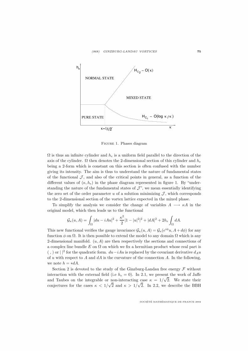
(868) GINZBURG-LANDAU VORTICES 75
PURE STATE
NORMAL STATE
MIXED STATE
H
H
heC
C
2
1∼
∼ O( κ)
O(log κ / κ )
κκ=1 / 2
Figure 1. Phases diagram
Ω is thus an infinite cylinder and he is a uniform field parallel to the direction of theaxis of the cylinder. Ω then denotes the 2-dimensional section of this cylinder and he
being a 2-form which is constant on this section is often confused with the numbergiving its intensity. The aim is thus to understand the nature of fundamental statesof the functional J , and also of the critical points in general, as a function of thedifferent values of (κ, he) in the phase diagram represented in figure 1. By “under-standing the nature of the fundamental states of J ”, we mean essentially identifyingthe zero set of the order parameter u of a solution minimizing J , which correspondsto the 2-dimensional section of the vortex lattice expected in the mixed phase.
To simplify the analysis we consider the change of variables A −→ κA in theoriginal model, which then leads us to the functional
Gκ(u, A) =∫
Ω
|du− iAu|2 +κ2
2|1− |u|2|2 + |dA|2 + 2he
∫Ω
dA.
This new functional verifies the gauge invariance Gκ(u, A) = Gκ(eiφu, A+ dφ) for anyfunction φ on Ω. It is then possible to extend the model to any domain Ω which is any2-dimensional manifold. (u, A) are then respectively the sections and connections ofa complex line bundle E on Ω on which we fix a hermitian product whose real part is( , ) or | |2 for the quadratic form. du−iAu is replaced by the covariant derivative dAu
of u with respect to A and dA is the curvature of the connection A. In the following,we note h = ∗dA.
Section 2 is devoted to the study of the Ginzburg-Landau free energy F withoutinteraction with the external field (i.e he = 0). In 2.1, we present the work of Jaffeand Taubes on the integrable or non-interacting case κ = 1/
√2. We state their
conjectures for the cases κ < 1/√
2 and κ > 1/√
2. In 2.2, we describe the BBH
SOCIETE MATHEMATIQUE DE FRANCE 2002

76 T. RIVIERE
asymptotic analysis (F. Bethuel, H. Brezis and F. Helein [BBH]) in the London limit:κ → +∞ which corresponds to the strongly repulsive case. In this limit, to which weshall restrict in the following, the vorticity phenomena appear more clearly; this caseis also close to many of the type II superconductors we have in practice, for whichthe a-dimensional parameter κ is very large. In section 2.3, we revisit the part playedby the renormalized energy W coming from the BBH asymptotic analysis used todescribe the critical points of F . Finally, we give answers to the conjectures of Jaffeand Taubes in the London limit and we extend them to more general cases. The thirdpart is devoted to the complete study of the functional G comprising the interactionterm with the external field. The vorticity is then no longer a fixed parameter asin the previous section but becomes a variable of the problem. The contents of thissection covers part of S. Serfaty’s PhD thesis, and the work she did in collaborationwith E. Sandier.
2. STUDY OF THE FREE ENERGY FUNCTIONAL F
2.1. The integrable or non-interacting case κ = 1/√
2
In [JT], A. Jaffe and C. Taubes study the critical points on R2 of the free energyfunctional
Fκ(u, A) =∫
R2|dAu|2 +
κ2
2|1− |u|2|2 + |dA|2
and which are solutions to the Euler equations
(1)
⎧⎪⎨⎪⎩d∗AdAu = κ2u(1− |u|2)
d∗dA = (iu, dAu)
where d∗A is the operator acting on the 1-forms η such as d∗Aη = d∗η+iA∧η. Supposingthat the intrinsic quantities |dAu|, |1− |u|| and dA are decreasing (polynomially), therenormalized magnetic field is an integer N
N =12π
∫R2
dA
which corresponds to the degree of u/|u| on circles of sufficiently large radii. This isknown as the homotopy class of the couple (u, A). For a given N , say N ≥ 0, it hasbeen observed by E.B. Bogomol’nyi [Bog] that, for the particular value κ = 1/
√2,
the functional F can be rewritten under the following form
Fκ(u, A)∫
R2|!(dA1u)−"(dA2u)|2 + |!(dA2u)−"(dA1u)|2
+| ∗ dA + 12 (|u|2 − 1)|2 + 2πN
ASTERISQUE 276
(868) GINZBURG-LANDAU VORTICES 77
(! denotes the real part and " the imaginary part of a complex number). One of theprincipal results of [JT] is then the following:
Theorem 2.1 ([JT]). — Any critical point (u, A) of F1/√
2 of finite energy has adefined homotopy class N and verifies
(2) F1/√
2(u, A) = 2π |N |.
In particular, it minimizes F1/√
2 in its homotopy class.
The proof of this result can be understood as follows. Consider a critical point(u, A) of Fk. From the Euler equations (1), we can deduce the following ellipticequations verified by the intrinsic quantities 1− |u|2 and h = ∗dA
(3)
⎧⎪⎨⎪⎩−∆
(1− |u|2)2
+ 2κ2|u|2 (1− |u|2)2
= |dAu|2
−∆h + |u|2h = (dAu; i ∗ dAu)
where −∆ = d∗d and
(dAu; i ∗ dAu) = −<!(dAu),"(∗dAu)> + <"(dAu),!(∗dAu)>
(< , > is the scalar product on the 1-forms). Using (3) we get from the maximumprinciple, on the one hand that |u| < 1 (unless |u| ≡ 1 on R2), and on the otherhand that the intrinsic quantities |h|, |dAu| and |1−|u|| decrease exponentially fast toinfinity, so that one has in particular a well defined homotopy class for (u, A). Theseexponential decreases have an important physical interpretation linked to the mass ofthe Higgs particle.
Another important ingredient to prove theorem 2.1 is the conservation law of theenergy-momentum tensor, which we shall use extensively throughout this talk. Theenergy-momentum tensor (Tij)i,j∈1,2 is given by
(4) Ti,j = 2δij |dA|2 + 2(dAiu, dAju)− δijfκ(u, A),
where fk(u, A) is the free energy density fκ(u, A) = |dAu|2 + κ2
2 |1 − |u|2|2 + |dA|2.The conservation law of this tensor results from the fact that (u, A) is on the onehand a critical point of Fk, and on the other hand C∞, which can be deduced fromthe Euler equations (1); it is thus also a critical point for variations of the domain.Using Noether theorem, the translational invariance of the domain then gives rise todivergence free quantities, which constitute this conservation law
(5) ∀j = 1, 2∂
∂xiTij = 0.
From this law, we can deduce the following Pohozaev identity, which is a consequenceof the fact that (u, A) is a critical point of the infinitesimal action of dilations r ∂
∂r (i.e
SOCIETE MATHEMATIQUE DE FRANCE 2002

78 T. RIVIERE
we multiply (5) by xj , sum on j and integrate over R2)
(6)∫
R2
κ2
2|1− |u|2|2 =
∫R2|dA|2.
Let us restrict ourselves to the case κ = 1/√
2. One can easily see that for thatparticular value of the parameter, by summing or subtracting the two equations of(3), the maximum principle leads to
(7) |dA| = |h| ≤ |1− |u|2|2
.
Moreover, for κ = 1/√
2, the Pohozaev identity becomes
(8)∫
R2
(1− |u|2
2− ∗dA
)(1− |u|2
2+ ∗dA
)= 0.
Excluding the simple case where |u| ≡ 1 (N = 0) and thus dA ≡ 0 from (6), wehave |u| < 1 and combining (7) and (8) gives either ∗dA = 1−|u|2
2 (for N > 0),
or ∗dA = − 1−|u|22 (for N < 0). Bootstrapping for example ∗dA = 1−|u|2
2 in theequations, one easily obtains that !(dA1u) = "(dA2u) and that !(dA2u) = "(dA1u),which together with the observation of Bogomol’nyi proves the theorem.
Theorem 1 tells us that solving the solutions of the second order equations, comesup in the case κ = 1/
√2 and for the class of configurations (u, A) of finite energy, to
the study of the solutions of the first order equations (for N > 0)
(9) ∗dA =1− |u|2
2
(10) !(dA2u) = "(dA1u)
(11) !(dA1u) = "(dA2u),
which justifies the fact that this case is called integrable. The qualitative study of thesolutions to these equations gives quite easily that the set of zeros of |u| is constitutedof a finite number of points where the index of u is strictly positive. We can thusrepresent it by exactly N points, not necessarily distinct from one another, x1...xNeach of multiplicity 1. We can then verify that v = log |u|2 is a solution of
(12) −∆v + ev − 1 = −4π
N∑k=1
δxkin D′(R2).
A convexity argument shows that the solution v to equation (12) is unique for anyconfiguration of points x1...xN. We easily bootstrap this uniqueness of |u| in equa-tions (9), (10) and (11) to deduce the uniqueness (up to the gauge action) of theconfiguration (u, A). We can then go the other way round, and taking N arbitrarypoints in the plane, exhibit a solution to (9)...(11). We have then proven the theoremenunciated below.
ASTERISQUE 276
(868) GINZBURG-LANDAU VORTICES 79
Theorem 2.2 ([JT]). — The space of the solutions of finite energy of the abelianYang-Mills-Higgs (1) in the plane, in the integrable case κ = 1/
√2, is nothing but (up
to the action of the gauge group) the space of configurations of points in the plane,having integer multiplicities, all of the same sign.
One of the striking points of the integrable case κ = 1/√
2, is that not only can thevortices (zeros of u) be anywhere in the plane, but that the energy of the solutionsis independent of the relative positions of the vortices, and is equal to 2π timesthe number of vortices. This is why the integrable case is also known as the non-interacting case. By handwaving arguments, A. Jaffe and C. Taubes conjecture thatκ = 1/
√2 is the limiting case between two opposite behaviors of vortices amongst
themselves; for κ < 1/√
2, whatever be their signs, the vortices have a tendency toattract one another, which justifies in some way the absence of a mixed phase, whilein the case κ > 1/
√2 the vortices with same signs should repel one another, but since
their presence is imposed by the energy input due to the external field (see section 3),this leads to the possibility of a mixed state (see figure 1). Precisely the conjectureof Jaffe and Taubes for the repulsive case (κ > 1/
√2) is as follows.
Conjecture 2.3 ([JT]). — For κ > 1/√
2, there exist stable solutions of YMH (1)on all R2 if and only if |N | = 1, 0; moreover they have an axial symmetry (up to thegauge action).
In both of the next sub-sections, we shall rigorously account for these expectedbehaviors of the vortices amongst themselves in the strongly repulsive case (κ → +∞)and give a partial answer to the conjecture 2.3 (see theorem 2.10).
2.2. The strongly repulsive case or “London limit” κ → +∞: the BBHasymptotic analysis
From now on, we shall study the behavior of the vortices in the strongly repulsivecase (κ → +∞). To prevent the vortices from separating from one another to infinity,we study F on a compact 2-dimensional manifold M without boundary, in order notto have to take artificial boundary conditions. For clarity, we shall restrict ourselves tothe case where M is a flat torus. In fact the metric on M , as well as its topology, doesnot modify the qualitative aspects of the results. We also take a hermitian complex linebundle on M whose Euler class e(E) verifies
∫M e(E) = N > 0, which implies that any
section u intersecting transversely the zero section, does it algebraically N times. Wethus fix the total vorticity of the problem, which becomes a parameter of the problem.In section 3 of this talk, we shall take into account the influence of the external field,so that the total vorticity will be once again a variable of the problem as in the originalmodel. The existence of a couple section-connection (uk, Ak) minimizing Fk in theSobolev spaces W 1,2 of sections and connections (the expression in a trivialization ofthe bundle of (u, A) gives the functions and 1-forms W 1,2) is now a classical problem
SOCIETE MATHEMATIQUE DE FRANCE 2002

80 T. RIVIERE
which requires the use of Coulomb gauges in order to render the functional coercitive(see [Uh]). We thus propose to study the behavior of such minimizing couples (uk, Ak)when κ tends to infinity. The difficulty of such an analysis comes from the fact thatwe do not dispose of estimates a priori sufficient, independent of κ, in any functionalspace, to prove any weak convergence towards something. In particular, we can verifythat Fκ(uk, Aκ)→ +∞ and more precisely we have
(13) Fκ(uκ, Aκ) 2πN log κ.
F. Bethuel, H. Brezis and F. Helein give a complete description of this asymptotic in[BBH] for the case A = 0 on a domain of R2 (this is completed in [St], adapted tothe gauge invariant model in [BR1] and later in [Qin], and followed the study of thesymmetric case on R2 in [BC]). They then establish the following result:
Theorem 2.4 ([BBH]). — Given a sequence of configurations (uκ, Aκ) minimizingFκ for a sequence of κ tending towards infinity, there exist a sub-sequence (u′
κ, A′κ)
and N distinct points p1...pN of M such that
(14) (uκ′ , Aκ′) −→ (u, A) in Ckloc(M)
where M = M \ p1...pN, (u, A) is a couple unitary section-connection of E overM , which is a critical point of the functional
(15) F(u, A) =∫
M
|dAu|2 + |dA|2.
Moreover the index of the singular A-harmonic section u at each pj is +1, whichgives in particular that the limiting curvature h = ∗dA verifies the“London equation”
(16) d∗dh + h = 2π
N∑k=1
δpkin D′(M).
Remark 1. — The positions of the limiting vortices p1...pN determine uniquely thecouple (u, A) (up to the gauge invariance).
We sketch the main points of the proof below—we omit the index κ.Again, the maximum principle applied to the first equation of (3) gives |u| ≤ 1.
Combining this L∞ bounding of |u| and the bounding of the configuration energy(u, A) given by (13), by means of classical elliptic estimates (in the spirit of inter-polation inequalities of the Gagliardo-Nirenberg type [BBH0]), we get the followingcontrol over the L∞ norm of the covariant derivative of u (which is actually optimal)
(17) ‖d|u|‖L∞(M) ≤ ‖dAu‖L∞(M) = O(κ).
The general strategy will consist in identifying and covering in the best possible waythe zero set of |u|, which coincides with the region of loss of compactness of the se-quence of configurations (u, A) in W 1,2. This region is called“bad set”; more precisely,
ASTERISQUE 276
(868) GINZBURG-LANDAU VORTICES 81
it refers to the following set:
(18) M = x ∈M such that |u|(x) < 1/2
(the constant 1/2 is in fact chosen arbitrarily between 0 and 1). We then have thefollowing “quantization” result.
There exists δ > 0 independent of κ such that, for all x0 in M ,
(19) κ2
∫Bκ−1 (x0)
|1− |u|2|2 ≤ δ =⇒ x0 /∈M.
This result is an immediate consequence of (17). It implies that a point of M con-tributes, on a ball of radius κ−1, to a “finite”part of the Higgs energy κ2
∫Bκ−1 (x0)
|1−|u|2|2 (i.e larger than a value δ > 0 independent of κ).
The joint use of the upper bounding of the energy and the conservation law of theenergy-momentum tensor (5), from which we deduce the Pohozaev identity on anygeodesic ball, gives in particular (cf [BR1])
(20) ∀0 < α < 1 ∀x ∈ M κ2
∫Bκ−α (x0)
|1− |u|2|2 ≤ Cα,
where Cα is independent of κ. The use of the intermediate scales κ−α in [BR1]between the natural scales of the problem (1 and κ−1) enables us to get rid of themagnetic field in the Pohozaev identities and to obtain (20). These scales (which arenot really necessary in the case A = 0 in dimension 2 [BBH]) are extensively used inthe gauge invariant model ([BR1], [Ri1], [Ri2]...). Combining (19) and (20), we getthe following covering of M on a whole ball of radius κ−α.
(21) ∀x ∈ M M∩Bκ−α(x) ⊂ ∪Nα
j=1Bκ−1(xj) and Nα = O(1)
where (xj)j∈1...Nα is a family of points in Bκ−α(x) et Nα and Nα is bounded inde-pendently of κ.
Once again, the use of the stress-energy tensor (5) enables us to prove the quanti-zation result below:
Lemma 2.5 (eta-compactness). — There exists η > 0 independent of κ such that forany radius 1 ≥ ρ ≥ κ−1 and any x in M , one has
(22)
∫Bρ(x)
fκ(u, A) ≤ η log(ρκ)
=⇒ Bρ/2(x) ∩M = ∅
where fκ(u, A) is the free energy density f(u, A) = |dAu|2 + κ2
2 |1− |u|2|2 + |dA|2.
This lemma tells us that the contribution of the bad set to the total energy ona ball of radius ρ is at least greater than η log(ρκ). The proof in 2 dimensions isquite straightforward (see [Ri1]), while in larger dimensions, it becomes much moretechnical (see [Ri2] [LR2]).
SOCIETE MATHEMATIQUE DE FRANCE 2002
82 T. RIVIERE
The combination of the bounding of the energy (13), (21) and the lemma of eta-compactness enables us to conclude easily that the set M is contained in a uniformnumber of bounded balls of radius κ−1:
(23) M⊂ ∪nj=1Bκ−1(xj) n = O(1).
We can then extract a sub-sequence of the original sequence κ → +∞ such that thefamily (xj)j=1..n converges in M .
Outside M, h = ∗dA verifies the following elliptic equation deduced from thesecond Ginzburg-Landau equation (1)
(24) d∗[
1|u|2 dh
]+ h = 0 in M \ ∪n
j=1Bκ−1(xj).
What prevents this equation from being verified on all M is the index of u aroundthe zero set. Then if dj =deg( u
|u| ; ∂Bκ−1(xj)), one verifies that
(25)∫
∂Bκ−1 (xj)
dh
|u|2 +∫
Bκ−1 (xj)
h = 2πdj .
From (24) and (25), we then have that h is a κ−1-approximation of the followinglinear problem
(26) d∗dk + k = 2π
n∑j=1
δxj .
From (17), we can deduce that the dj are uniformly bounded and thus that theW 1,p norms (p < 2) of k are bounded independently of κ. These boundings can betransmitted easily to h = ∗dA and by bootstrapping then in the Ginzburg-Landauequations (1), we prove theorem 2.4 (moreover to show that n = N , we have used theminimality of the solution).
As opposed to the non-interacting case κ = 1/√
2, the vortices xj and their limits(p1...pN ) cannot be anywhere in the domain M , the configuration (p1...pN ) minimizesa certain energy W of MN \∆ in R, known as the renormalized energy (∆ denotesthe diagonal of MN ).
Theorem 2.6 ([BBH]). — The configuration of limiting vortices (p1...pN ) given bytheorem 2.4 is a fundamental state of the following function defined on MN \∆
(27)W (z1...zN ) = 2
∑i=j
∫M
dGi · dGj + 2N∑
j=1
∫M
dR · dGj
+∫
M
|dR|2 +∫
M
|k|2.
The fact that the vortices strongly repel one another can be clearly seen in W .Indeed, we can verify that if two vortices zi and zj come close to each other, theothers remaining fix, then we have W 2π log |zi − zj|.
ASTERISQUE 276

(868) GINZBURG-LANDAU VORTICES 83
The proof of theorem 2.6 relies on the following decomposition. We take someδ > 0 independent of κ. We divide M into two disjoint parts M = ∪N
k=1Bδ(pk)∪Mδ.We decompose the total energy as a sum of the energies on each ball Bδ(pk) andon Mδ. According to theorem 2.4, |u| converges uniformly towards 1 while ∗dA
converges uniformly towards h which is solution of (16) on Mδ. Using then thesecond Ginzburg-Landau equation, we get
(28) limκ→+∞
∫Mδ
fκ(u, A) =∫
Mδ
|dh|2 + |h|2.
Moreover, an explicit calculation enables us to verify that
(29) limδ→0
∫Mδ
|dh|2 + |h|2 − 2πN log1δ
= W (p1...pN ) + C,
where C is independent of the positions of the vortices. Using a covering of M by afinite number of balls of radii κ−1, we can show by means of the convergence givenby theorem 2.4 that the principal part of the energy around a limiting vortex isindependent of its position and of the existence of the other vortices
(30)∫
Bδ(pk)
fκ(u, A) = 2π log(δκ) + C0 + oδ(1),
where C0 is a universal constant. By combining (28), (29) and (30) we can easilyverify that to optimize Fκ, we have to optimize the configuration of vortices (p1...pN)with respect to W . This proves theorem 4.
Moreover, we have shown that Fκ(uκ, Aκ) has the following asymptotic expansion.
(31) Fκ(uκ, Aκ) = 2πN log κ + W (p1...pN ) + C0N + o(1).
This asymptotic expansion can be interpreted as follows: each vortex interacts withitself with an energy with principal part 2π log κ, W is the interaction energy amongstvortices, and finally C0 is the renormalized energy of an isolated particle.
If we now follow a sequence (uκ, Aκ) of Ginzburg-Landau solutions (1) in the“London limit” (κ → +∞), which is now not necessarily a sequence of minima, weprove results corresponding to theorems 2.4 and 2.6, the condition being to remainin “reasonable” energy levels Fκ(uκ, Aκ) = O(log κ). The number of limiting vorticesp1...pQ is now not necessarily N . To each vortex is associated an integer multiplicitydj which is the index of the limiting singular section u around pj . The equationverified by the limiting field h becomes
(32) d∗dh + h = 2π
Q∑j=1
djδpj in D′(M)
while the positions of the pj is a critical point of the function W given by (27) whereGj is replaced by djGj .
SOCIETE MATHEMATIQUE DE FRANCE 2002

84 T. RIVIERE
2.3. The space of solutions in the “London limit”
Study of the zero set in the London limit. — We saw that in the London limit (κ →+∞), the zero set of the minimizing section uk is forced to converge towards a veryprecise locus of points of the domain: p1...pN which is a critical point of the functionW . We now want to have a more complete description of this zero set, and eventually,to see in which limit the property obtained in the non-interactive case, saying that twosolutions having the same zeros are gauge equivalent, remains valid in the stronglyrepulsive case. This would then bring the study of the space of solutions to that of theeventual zero set and would justify the tendency in physics to call Ginzburg-Landauvortices the solutions to the Ginzburg-Landau equations themselves.
Consider a sequence of minima (uκ, Aκ) of Fk converging as in theorem 2.2 towardsa couple section-singular connections (u, A). We first look for the zero set of |uκ|—we shall omit the index κ except where necessary. The limiting section being of index1 to p1, the sum of the indices of u on the bad balls Bκ−1(xi) converging towards p1
is also +1. We can always suppose that |u|(xj) < 1/2.
If ever the centers xl and xk of two bad balls separate faster that O(κ−1), we obtaina contradiction for the following reason. Suppose that this actually occurs, then upto the extraction of a sub-sequence, we can suppose that
(33) κ|xk − xl| −→ +∞.
Consider then the dilation of the section around the point xk given by (in a localCoulomb gauge): uκ(z) = u(κ−1z + xk). The convergence of the field dA establishedin the proof of theorem 2.4 as well as in the L∞ bound of the covariant derivative(17) enable to conclude that, up to an extraction of a sub-sequence, uκ converges inC1
loc(R2) towards a solution of
(34)
⎧⎪⎪⎪⎪⎪⎪⎪⎨⎪⎪⎪⎪⎪⎪⎪⎩
∆u + u(1− |u|2) = 0 on R2
|u|(0) < 1∫R2|1− |u|2|2 < +∞.
It is shown in [BMR] that the Higgs energy of the solutions of (34) is quantized:
(35)∫
R2|1− |u|2|2 ∈ 2πN∗.
Thus, if we go back to the original scale, for a sufficiently large radius R, independentof κ, with κ sufficiently large, then at the limit the contribution of the ball Bκ−1R(xk)to the Higgs energy is at least 2π. This also holds for xl and thus, since both pointsseparate faster than O(κ), from (33) we can deduce that for all δ > 0 independent of
ASTERISQUE 276
(868) GINZBURG-LANDAU VORTICES 85
κ
(36) lim infκ→+∞
κ2
∫Bδ(p1)
|1− |uκ|2|2 ≥ 4π.
Moreover, the Pohozaev identity on the ball Bδ(p1) deduced from the energy-momentum conservation law, combined with the convergences of theorem 2.4, easilygives
(37) limκ→+∞
κ2
∫Bδ(p1)
|1 − |uκ|2|2 = 2π + oδ(1).
(36) and (37) are then in contradiction, and so (33) cannot occur even for a sub-sequence. Thus, there exists λ > 0 independent of κ such that the part of the badset M converging towards p1 can be covered by exactly one ball of radius λκ−1.So let x1 be the center of this ball and more generally xi be the center of the ballconverging towards pi and containing M in the vicinity of pi. We can always supposethat u(xi) = 0 since the limiting index of u is non-zero at pi, but equal to 1, and thatu must become 0 somewhere in the part of M which converges towards pi which iscontained in Bλκ−1(xi). The dilation argument previously applied from x1 then saysthat, in a local Coulomb gauge, uκ(z) = uκ(κz + x1) converges in C1
loc(R2) up to the
extraction of a sub-sequence towards a solution u of the following problem.
(38)
⎧⎪⎪⎪⎪⎪⎪⎪⎪⎪⎪⎨⎪⎪⎪⎪⎪⎪⎪⎪⎪⎪⎩
∆u + u(1− |u|2) = 0 in R2
|u(0)| = 0∫R2|1− |u|2|2 < +∞
ind(u, +∞) = +1.
(It is shown in [BMR] that from the first three lines of (38), one can show that|u| converges uniformly towards 1 at infinity and thus that the index u, ind(u, +∞)is well-defined.) Equation (38) is known as the “profile” equation of the Ginzburg-Landau vortices. The problem of the multiplicity of the solutions of (38) is not astandard problem in non-linear elliptic equations; indeed u does take real but complexvalues and the classical approaches using the maximum principle to show an eventualsymmetry of the solution cannot apply here.
P. Mironescu in [Mi] gave the following proof of the uniqueness (up to rotations)of the “profile”.
It is quite standard to verify that there exists a unique solution of (38) of the formρ(r)eiθ ((r, θ) being the polar co-ordinates on R2). Let us divide u, which is anysolution of (38), by this axially symmetric solution. The ratio w = u/ρ(r)eiθ is a
SOCIETE MATHEMATIQUE DE FRANCE 2002
86 T. RIVIERE
critical point on R2 \ 0 of the functional
E(w) =∫
ρ2|∇w|2 + 2ρ2
r
(iw,
∂w
∂θ
)+ ρ4|1− |w|2|2.
w is the critical point for the infinitesimal action of dilations r ∂∂r on R2 \ 0. This
then gives the Pohozaev identity
(39) 0 =∫
R2rρ′
ρ
∣∣∣∣∂w
∂r
∣∣∣∣2 +rρρ′ + ρ2
2|1− |w|2|2
(the index 1 being used at infinity to get rid of the boundary terms). A simple studyof the modulus of the radial solution ρ enables to conclude that ρ′ > 0. The identity(39) then tells us that |w| = 1, ∂w
∂r = 0 and thus u = ρ(r)ei(θ+α) where α is a constant.This proves the uniqueness of the profile up to rotations.
Since uκ converges (up to the extraction of a sub-sequence) in C1loc(R
2) towardsthis profile (unique up to rotations), also since u becomes zero exactly at 0 and since∇2u(0) has rank 2, one can then verify that on Bλ(0) u−1
k (0) = 0. Thus on theball Bδ(p1), u is equal to zero at a unique point.
We have up to now used the fact that the couple (uκ, Aκ) is minimal in orderto get the convergence of theorem 2.4 and the index 1 of u at each pj . From theextension of the results 2.4 and 2.6 to any of the critical configurations (uκ, A,κ )under the energy levels O(log(κ)) described at the end of section 2.2, we have shownthe following proposition.
Proposition 2.7. — Let (uκ, Ak) be a sequence of configurations (κ → +∞),solutions of the Ginzburg-Landau equation (1), verifying the energy boundingFκ(uκ, Aκ) = O(log κ) and converging towards a couple section-connection (u, A)singular at p1...pQ. If the index of u at pj is ±1 for all j, then there exists κ0 suchthat for κ > κ0, we have
|uκ|−1(0) = x1...xQ and xj − pj → 0 for all j.
The role of the renormalized energy W . — Let us again place ourselves in the hy-potheses of proposition 2.7. The section uκ for κ sufficiently large thus intersectsexactly Q times the zero section with each time an intersection index ±1. Each ofthose zero points of |uk| converges towards a limiting vortex p1...pQ. Considering howimportant the part played by the position of the zero is in P. Mironescu’s uniquenessargument, a natural question is whether, more generally, two solutions of (1) hav-ing the same zero sets in the London limit, are equal (up to the gauge invariance).This proposition would generalize to the strongly repulsive case the same propositionproved above by Jaffe and Taubes for the non-interacting case. The answer to thisquestion is yes under the same hypotheses as in proposition 2.7.
ASTERISQUE 276

(868) GINZBURG-LANDAU VORTICES 87
Proposition 2.8 ([PR]). — Let (uκ, Aκ) and (vκ, Bκ) be two sequences of solutionsof the Ginzburg-Landau equations (1) in the London limit (κ → +∞) verifying thecommon energy bounding Fκ(uκ, Ak) = O(log κ) , Fκ(vk, Bk) = O(log κ), and bothconverging towards the same singular configuration (u, A). We suppose that theindex of u at each singularity is ±1. Then there exists κ0 such that for κ > κ0
|uκ|−1(0) = |vκ|−1(0) =⇒ (uκ, Aκ) (vκ, Bκ),
where denotes the gauge equivalence.
The proof of the preceding proposition relies amongst other things on the followinggeneralization of P. Mironesu’s argument. In a Coulomb gauge in the vicinity of anylimiting vortex pk, we reconsider under the hypotheses of the proposition, the ratio ofthe two solutions w = u
v . Instead of making dilations with respect to the conformalfield X = r ∂
∂r centered at the common zero of u and v, which do not give any resultsin that case, we dilate with respect to the following field, constructed from the secondsolution of v,
Y = |v|2 (iv, ∗dv)|(iv, ∗dv)|2
where we identify the field with the dual 1-form given by the scalar product. We canobserve that Y coincides with the usual conformal dilation field X = r ∂
∂r in the casewhere v has a radial symmetry. The action of this field on the functional for which(w, A) is a critical point gives a Pohozaev identity in the vicinity of pk, which all puttogether enable us to conclude that for sufficiently large κ (uκ, Aκ) (vκ, Bκ).
The use of Y rather that the usual field X = r ∂∂r is a posteriori natural in view of
the functional for which (w, A) is a critical point and of the property of |v|-conformalityof Y (see [PR]).
The proposition 2.8 is the first step to describe the space of solutions below theO(log κ) energy levels in the London limit. The second step consists in constructinga sequence (vκ, Bκ) converging towards a (u, A) whose configuration of associatedvortices p1...pQ is any critical point of W (non-degenerate up to the actions of isome-tries of M) and whose multiplicities dj are ±1. Such a construction has been done in[LL] for dj = +1 by means of variational arguments, by establishing a link betweenthe level sets of the function W and the functional Fκ. In [PR] this construction isdone for dj = ±1 by means of the local inversion theorem which also has the advan-tage to bring the local uniqueness. The argument of linearization around a solution isrendered complex by the existence of a“kernel at infinity”: the inverse of the linearizedoperator of (1) around an accumulation of vortices which converges towards (u, A),blows-up in the standard norms W 2,2−L2 when κ tends to infinity. This is due to theaction of the invariance group of the limiting profile equation (38) (here the isometriesof the plane). We are thus led to develop the Lyapunov-Schmidt reduction argumentwhich first consists in working in a direction perpendicular to this kernel at infinity,which we reintroduce in the final non-linear argument. This technique applied to the
SOCIETE MATHEMATIQUE DE FRANCE 2002

88 T. RIVIERE
elliptic P.D.E. has often been used in a number of constructive problems of differentialgeometry like the existence of minimal surfaces, the existence of surfaces of constantmean curvature, the Yamabe problem, the Yang-Mills monopoles... by N. Kapouleas,R. Mazzeo, F. Pacard, R. Schoen, K. Uhlenbeck, S.T. Yau... with each time newdifficulties. (vκ, Bκ) being thus constructed benefits from a local uniqueness in anadapted functional space. If (uκ, Aκ) is another solution of (1), converging towardsthe same limiting configuration whose singularities are p1...pQ, we know (proposi-tion 2.7) that the zeros of |uκ| converge towards those singularities and are thus closeto those of |vκ|. The argument of the proof of proposition 2.8 is then converted inorder to obtain, no longer directly that (uκ, Aκ) (vκ, Bκ), a sufficiently small boundof the “separation” of (uκ, Aκ) and (vκ, Bκ) which, by means of the local uniquenessestablished previously, enables to conclude that (uκ, Aκ) (vκ, Bκ). We thus havethe following theorem.
Theorem 2.9 ([PR]). — Let (p1...pQ) be a critical point of the renormalized energyW for the multiplicities (d1...dQ) in −1, +1. Suppose that this critical point isnon-degenerate up to the action of isometries of M . Let (u, A) be the singularcouple section-connection associated to (pj , dj). Then let (uκ, Aκ) and (vκ, Bκ) be twosequences of Ginzburg-Landau equations (1) verifying the common energy boundingFκ(uκ, Aκ) = O(log κ) and Fκ(vκ, Bκ) = O(log κ), if their singular closure set is theconfiguration (u, A), then for sufficiently large κ
(uκ, Aκ) (vκ, Bκ)
up to the action of isometries of M ( is the gauge equivalence).
Comments. — Theorem 2.9 tells us that under certain hypotheses, the study ofthe critical points of the functional Fκ in the London limit—infinite dimensionalproblem—can be brought to that of the critical points of the function W—finite di-mensional problem. The limits of our description of solutions to the Ginzburg-Landauequations in the strongly repulsive case are the following. First, in order to be in thecontext of the BBH asymptotic, we have restricted the critical points to energies belowC log κ. How about other eventual solutions to (1)? In the case A = 0 on a star-shaped domain, it has been shown that all the Ginzburg-Landau solutions are under acertain energy level C log κ. The second restriction in the hypotheses of theorem 2.9 isthe constraint on the limiting multiplicities dj who have to belong to +1,−1. Howabout the branches of solutions linking a critical point of W where some of |dj |’s aregreater than 1? This question is completely open. Neither the variational methods,in the spirit of [LL], or [AB1], [AB2], nor critical points methods, seen above, haveenabled up to now the construction of solutions (other than the axially symmetricsolutions) converging towards a critical point of W with multiplicities dj = ±1. Wedo not even have a precise idea of the aspect of such solutions near the vortices.The understanding of the possible limiting “profiles” is also lacking in that case (see
ASTERISQUE 276

(868) GINZBURG-LANDAU VORTICES 89
conjectures on that theme in [OS]). Nevertheless, it seems that the case dj = ±1 is“generic” in the following sense: for a “generic” perturbation of the metric, a criticalpoint of W having multiplicity indices greater than 1 should be transformed into acritical point whose indices are ±1.
To end up the study of the free energy, we should mention that the techniquespresented above help to bring a partial answer to the Jaffe and Taubes conjectureson all R2 in the strongly repulsive case.
Theorem 2.10 ([Ri3]). — The conjecture 2.3 is true in the London limit (sufficientlylarge κ) if we replace “stable critical point” by “minimum in the homotopy class”.
3. INTERACTION WITH AN EXTERNAL MAGNETIC FIELD;TOWARDS THE ABRIKOSOV LATTICES
3.1. Introduction
Up to now, we have studied the Ginzburg-Landau free energy Fκ without theinteraction term with the magnetic field 2he
∫dA. Moreover, we have placed ourselves
on a plane torus in order to ignore in a first approach, the border effects which arehowever very important in phenomenological studies, and about which it would bevery interesting to recover the conclusions by the mathematical study itself. Finally, inthe absence of external magnetic field, in order not to work with a trivial fundamentalstate, we have imposed a global vorticity through the choice of a certain bundle onour torus of non zero Euler class. The analysis of our model problem has enabled usto isolate and understand the mechanism
vorticity =⇒ vortex formation
and to bring the study of the space of solutions to that of the positions of the vortices,governed by the renormalized energy.
In her PhD thesis [Se1], then in her works in collaboration with E. Sandier [SS1][SS2], S. Serfaty considers the complete functional Gκ including the interaction termwith the external magnetic field, on Ω a simply connected bounded domain of R2.The vorticity is thus free and should spontaneously appear by increasing the externalmagnetic field and thus the total free energy of the system as it has been observedfor type II superconductors (κ > 1/
√2).
We still place ourselves in the London limit (κ −→ +∞) and the magnetic field he
is assumed to be uniform (we will confuse the 2-form and the corresponding constant).
SOCIETE MATHEMATIQUE DE FRANCE 2002
90 T. RIVIERE
3.2. The Meissner solution
When the applied field he = 0, the fundamental state of Gκ is clearly reached by thepure state solution h = ∗dA = 0. When we increase the field he, the superconductingcharacter of the sample changes a little without however forming any vortex (|uκ| ≥1/2 for sufficiently large κ). We expect this configuration which is vortex-free, stable,and absolute minimum for not too strong external fields, to be unique. This is whatS. Serfaty shows by combining energy estimates and convexity arguments.
Theorem 3.1 ([Se3]). — In the London limit (κ sufficiently large), there exists aunique stable, vortex free (|uκ| ≥ 1/2) critical point of Gκ which minimizes Gκ amongstthe vortex-free critical points, with the condition he = O(κα) where α is a positiveconstant. This solution known as the “Meissner solution” verifies in particular
(40)
⎧⎪⎨⎪⎩−div(∇h
|u|2
)+ h = 0 in Ω
h = he on ∂Ω.
The constant 1/2 is of course a constant chosen at random between 0 and 1. Infact the Meissner solution remains stable up to a critical value of the applied fieldhe = Hsh Cκ known as the “super-heating field”, and above which it is no longerstable. This separation has been studied in detail by H. Berestycki, A. Bonnet andJ. Chapman in [BBC]. Moreover, the uniqueness of the Meissner solution in thevicinity of the field Hsh is proven by A. Bonnet, J. Chapman and R. Monneau in[BCM].
What is then natural to ask oneself is for which value Hc1 of the external field he,the Meissner solution ceases to be a minimum of Gκ. The calculations of Abrikosov onall R2 predict Hc1 log κ
2 . As we shall see, the work of S. Serfaty has enabled to show,that following a conjecture in [BR2], Hc1 is in fact larger on a bounded domain. Thisis a consequence of border effects and is more precisely as follows: in the principalterm of Hc1 , the factor 1/2 in front of log κ has to be replaced by k1 = 1/2 max |ξ0|where ξ0 is the solution of
(41)
⎧⎪⎨⎪⎩∆ξ0 = ξ0 + 1 in Ω
ξ0 = 0 on ∂Ω.
ξ0 is also solution of −∆2ξ0 + ∆ξ0 = 0. We can easily verify using the maximumprinciple that ∆ξ0 > 1 and ξ0 < 0 inside Ω and thus that |ξ0| < 1. E. Sandier andS. Serfaty then show the following result.
Theorem 3.2 ([SS1]). — There exists a constant C1 > 0 such that if
he ≤ k1 log κ− C1 log log κ
ASTERISQUE 276

(868) GINZBURG-LANDAU VORTICES 91
the Meissner solution is an absolute solution of Gκ and there exists C2 such that if
he ≥ k1 log κ + C2
the Meissner solution is no longer an absolute minimum of Gκ.
It is then tempting to place oneself in the vicinity of k1 log κ and to try to observethe vortices appearing one after the other as the external field is increased. Technically,this implies that we should work with the absolute minimum of Gκ for which we wouldtry to cover precisely the “bad set”M, in the spirit of the BBH asymptotic, by meansof uniformly bounded number of balls of radii κ−1 of which we would then studythe minimal value (eventually 0) and the energetically most advantageous respectivepositions.
With the above scheme, we unfortunately come across a major difficulty which hasnot yet been solved and which is exposed in the next section. The BBH analysis wasbuilt on the initial estimate of the free energy Fκ(uκ, Ak) = O(log κ) which can beexpressed by a bound of the number of vortices a priori independent of κ (knowingthat the cost for one “isolated” vortex is about 2π log κ). In the case we are actuallyconsidering, where the total vorticity is moreover not under control and has becomea variable of the problem, the bound of the energy is a priori
(42) |Gk(uκ, Aκ)| = O(log2 κ).
From that we cannot deduce a better estimate than Fκ(uκ, Aκ) = O(log2 κ) for thefree energy part. This thus tells us that the number of vortices that have to beconsidered a priori is O(log κ) (which must be true for a field he = 2k1 log κ, butnot for he = k1 log κ + O(1) where we expect rather a uniformly bounded numberof vortices). The difficulty of working with an a priori so large number of vorticesis responsible for the fact that we have to get out the BBH asymptotic scheme andthat the lack of precision is larger as can be seen between k1 log κ − C log log κ andk1 log κ + C2 in theorem 3.2 which is yet a very nice achievement.
The proof of theorem 3.2 has its roots in the asymptotic arguments of the previoussection. The point is to realize the best possible lower bound of the total energy ofa critical configuration with vortices and to show that for a sufficiently low externalfield, the Meissner solution is energetically preferable. In order to obtain such a lowerbound, we begin by renormalizing the induced field by “extracting” the external fielddescribed following [BR2]. Let ξ be the solution ∆ξ = h on Ω, which is equal to 0 on∂Ω (A = ∗dξ is the Coulomb gauge of h on Ω), we note ζ the difference ζ = ξ − heξ0
(where ξ0 is given by (41)). ∗dζ is the Coulomb connection on all Ω, from which wehave removed the influence of the external field. We show without much difficulty
SOCIETE MATHEMATIQUE DE FRANCE 2002
92 T. RIVIERE
that the energy of the minimal configuration (uκ, Aκ) can be decomposed as follows:
(43)
Gκ(u, A) = Gκ(1, he ∗ dξ0) + Fκ(u, ∗dζ) +∫
Ω
|∆ζ|2
−2he
∫Ω
(iu, du) ∧ dξ0 + o(1).
We suppose then that he = O(log κ) and we proceed to a decomposition of the domain,in the same spirit as that used to prove theorem 2.6, but more complex in the presentcase where the “bad set” is a priori far much bigger. We shall have Ω = Ωs∪Ωv whereΩs and Ωv are disjoint and Ωv will be a union of disjoint balls Bri(ai)i∈I coveringM, the “bad set”, and containing as much self energy as possible, without taking intoaccount the interaction energy of the vortices amongst themselves as in the proof oftheorem 2.6. Precisely, by means of a technique introduced by R. Jerrard [J], we show(see [SS1]) the existence of a family of balls B = Bri(ai)i∈I such that
– M⊂ ∪i∈IBri(ai)
–∫
Bri(ai)
fκ(u, ∗dζ) ≥ 2π|di| (log κ−O(log log κ)) where di =deg(
u|u| ; ∂Bri(ai)
)– ri = O(log−6 κ)– Card I = O(log2 κ).
We then choose Ωv = ∪i∈IBri(ai). The O(log−6 κ) radii replace the radii δ = O(1) ofthe proof of theorem 2.6 since the number of vortices tends towards infinity a priorias O(log κ). The role of the ai is a bit like intermediate vortices of degree di and thischoice of covering gives in particular
(44)∫
Ω
(iu, du) ∧ dξ0 = 2π∑i∈I
diξ0(ai) + o(1).
Combining (43), the choice of Ωv, (44) and the minimizing character of (u, A) for Gκ,we have
(45) 0 ≥ 2π∑i∈I
|di|(log κ + O(log log κ))− 4π he max |ξ0|(∑
i∈I
|di|)
and so if∑
i∈I |di| = 0, we must get he ≥ k1 log κ + O(log log κ), which establishesthe first part of theorem 3.2. The second part will be a consequence of theorem 3.3.
This technique of extracting the external magnetic field and then decomposing thedomain in order to optimize the lower bound of the energy is a recurrent theme inthe work of E. Sandier and S. Serfaty and appears through different forms to provethe theorems below.
3.3. Family of stable solutions having 1, 2, 3...vortices; the blooming of thelattice
For a while, let us give up the idea of considering the absolute minimum of Gκ, butyet keeping an external field in the vicinity of k1 log κ.
ASTERISQUE 276
(868) GINZBURG-LANDAU VORTICES 93
In her first work [Se1], S. Serfaty constructs a family of stable solutions whichhave a finite number of vortices for the fields 1 % he % κα (α being positive nonexplicit constant). To counteract the difficulty of showing evidence of a finite num-ber of vortices for the fundamental states themselves, S. Serfaty makes an ansatzwhich consists in considering, instead of the absolute minimum (uκ, Aκ) of Gκ in allW 1,2(Ω, C)×W 1,2(Ω, R2), the (uκ, Aκ) contained in the following set.
Dn =u ∈W 1,2(Ω, C) such that 2πn log κ + B ≤ Fκ(uT ) ≤ (2πn + 1) log κ
where
Fκ(uT ) =∫
Ω
|duT |2 +κ2
2|1− |uT |2|2.
uT is the projection of the function u on the unitary disc (uT = u if |u| ≤ 1 anduT = u/|u| otherwise) and B is a negative constant which remains fixed throughoutthe proof. The idea is that, in the Coulomb gauge on Ω, the cost for a vortex is(Fκ(uT ) 2π log κ). Thus, restraining to Dn, we a priori constrain the configuration(u, A) not to have more than n vortices so that we can get back to the BBH asymptoticin order to establish a complete description of (u, A). The main difficulty of thisapproach comes from the fact that it is not at all evident that a minimum of Gκ inDn, once we have established its existence, should be in the interior of Dn and thusbe a solution of the Ginzburg-Landau equation (1). Suppose that we have proven theexistence of a minimum (uκ, Aκ) of Gκ in Dn. We are tempted to use once more thearguments of section 2 to cover the “bad set”M... in order to establish an asymptoticexpansion of Fκ(uκ, Aκ) as in (31) and verify that (uκ, Ak) is well in the interior ofDn (i.e. 2πn log κ + B < F (uT ) < (2πn + 1) logκ) and thus solution of (1). Thedifficulty of this approach resides in the fact that as long as we do not know that(u, A) is solution of (1), we do not have an estimate of the form ‖d|u|‖L∞ = O(κ),no longer dispose of the quantization result (19) and the set M can be very diffuse,etc. We also no longer have any control of its size, which was given in section 2 byPohozaev identities. The idea is then, not to work any longer with (u, A) itself, butwith its parabolic regularization v which minimizes
minv∈H1(Ω,C)
∫Ω
|∇v|2 +κ2
2|1− |v|2|2 + κ2γ
∫Ω
|uκ − v|2
for some γ > 0. The advantage of replacing u by its parabolic regularisation v is that(v, A) will both be energetically very close to (u, A) and benefit from the propertiesof the minimum of Fκ in section 2 (such as |v| ≤ 1, |d|v|| = O(κ)...) which comefrom the elliptic equation verified by v. This idea of the parabolic regularization hasbeen introduced in the context of Ginzburg-Landau equations by L. Almeida andF. Bethuel in [AB2], in order to define an approximated configuration of vortices forany function u in the energy zone F (u) = O(log κ). We then establish an asymptoticexpansion for v in the spirit of section 2.2, which enables to deduce that (v, A) (andthus (u, A) too) which is energetically close to it, is in the interior ofDn. The existence
SOCIETE MATHEMATIQUE DE FRANCE 2002
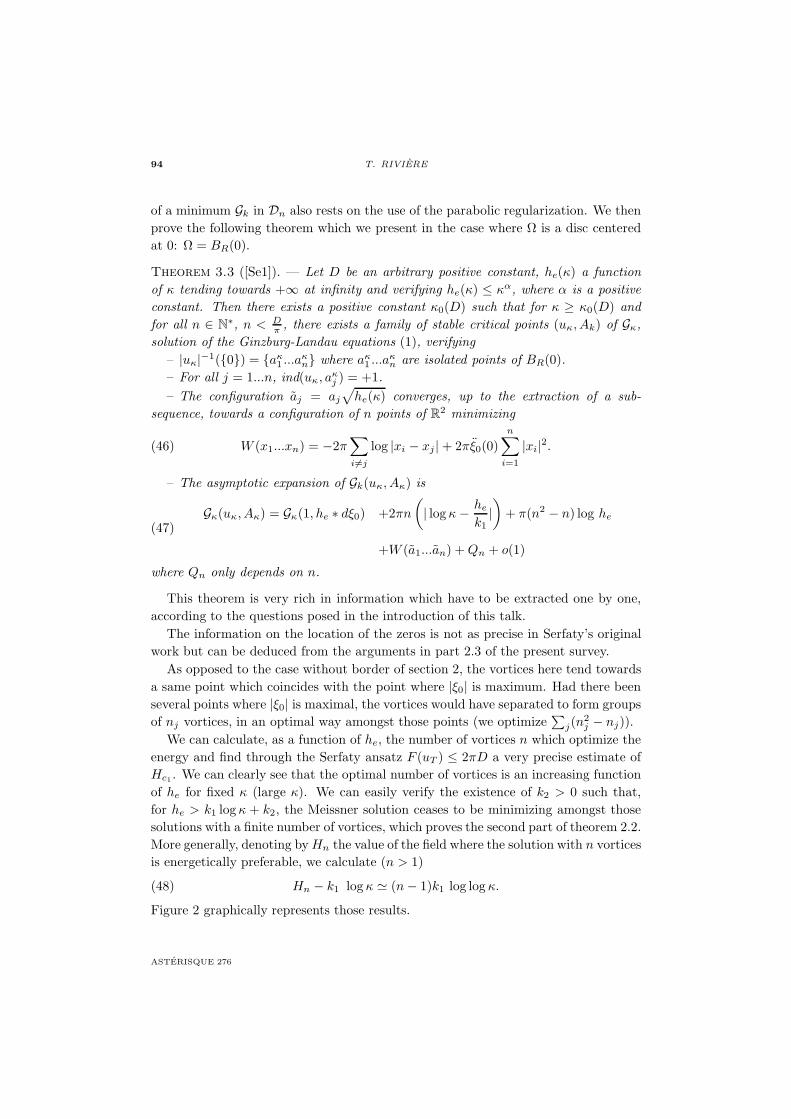
94 T. RIVIERE
of a minimum Gk in Dn also rests on the use of the parabolic regularization. We thenprove the following theorem which we present in the case where Ω is a disc centeredat 0: Ω = BR(0).
Theorem 3.3 ([Se1]). — Let D be an arbitrary positive constant, he(κ) a functionof κ tending towards +∞ at infinity and verifying he(κ) ≤ κα, where α is a positiveconstant. Then there exists a positive constant κ0(D) such that for κ ≥ κ0(D) andfor all n ∈ N∗, n < D
π , there exists a family of stable critical points (uκ, Ak) of Gκ,solution of the Ginzburg-Landau equations (1), verifying
– |uκ|−1(0) = aκ1 ...aκ
n where aκ1 ...aκ
n are isolated points of BR(0).– For all j = 1...n, ind(uκ, aκ
j ) = +1.– The configuration aj = aj
√he(κ) converges, up to the extraction of a sub-
sequence, towards a configuration of n points of R2 minimizing
(46) W (x1...xn) = −2π∑i=j
log |xi − xj |+ 2πξ0(0)n∑
i=1
|xi|2.
– The asymptotic expansion of Gk(uκ, Aκ) is
(47)Gκ(uκ, Aκ) = Gκ(1, he ∗ dξ0) +2πn
(| log κ− he
k1|)
+ π(n2 − n) log he
+W (a1...an) + Qn + o(1)
where Qn only depends on n.
This theorem is very rich in information which have to be extracted one by one,according to the questions posed in the introduction of this talk.
The information on the location of the zeros is not as precise in Serfaty’s originalwork but can be deduced from the arguments in part 2.3 of the present survey.
As opposed to the case without border of section 2, the vortices here tend towardsa same point which coincides with the point where |ξ0| is maximum. Had there beenseveral points where |ξ0| is maximal, the vortices would have separated to form groupsof nj vortices, in an optimal way amongst those points (we optimize
∑j(n
2j − nj)).
We can calculate, as a function of he, the number of vortices n which optimize theenergy and find through the Serfaty ansatz F (uT ) ≤ 2πD a very precise estimate ofHc1 . We can clearly see that the optimal number of vortices is an increasing functionof he for fixed κ (large κ). We can easily verify the existence of k2 > 0 such that,for he > k1 log κ + k2, the Meissner solution ceases to be minimizing amongst thosesolutions with a finite number of vortices, which proves the second part of theorem 2.2.More generally, denoting by Hn the value of the field where the solution with n vorticesis energetically preferable, we calculate (n > 1)
(48) Hn − k1 log κ (n− 1)k1 log log κ.
Figure 2 graphically represents those results.
ASTERISQUE 276

(868) GINZBURG-LANDAU VORTICES 95
H H H2 3c1he
Meissner sol.
1-vortex sol.
2-vortex sol.
3-vortex sol
Gκ
Figure 2. Solutions with 1,2,3... vortex
To know if the solution with n vortices for Hn ≤ he ≤ Hn+1 is a fundamentalstate on the whole space is an open seemingly difficult problem discussed in the nextsubsection. An important point is also the stable character of these solutions provenfor 1 % he % κα and which we have seen above for the Meissner solution and the“super-heating”field. This stability is responsible for hysteric phenomena observed inexperiments. The stable character of the solutions having a finite number of vorticesfor fields smaller than Hc1 has been observed by Q. Du and F.H. Lin in [DL].
Although the expression for the renormalized energy W is relatively simple, theeventual symmetries of its fundamental states, which constitute the bloomings of theAbrikosov lattices, are still to be completely explored. In [GS], S. Gueron et I. Shafrirhave done stability analyses of the symmetric configurations as well as numericalstudies. They have made the following observations on the probable fundamentalstates (see figure 3)
– n ≤ 3: these are regular polygons centered in 0– 7 ≤ n ≤ 10: these are regular, star-shaped (regular polygon + origin)– 4 ≤ n ≤ 6: the two previous types of configurations are locally minimizing and
are observed– n ≥ 11: these are clusters of regular concentric polygons which “converge” to-
wards a triangular lattice centered in 0 when n becomes large.
3.4. An interesting open problem: remove S. Serfaty’s Ansatz
It would be nice to really characterize the phase change at Hc1 through a rigorousproof of the spontaneous creation of vorticity for absolute minimizers. In other wordsan interesting question would be to remove S. Serfaty ansatz and to replace the
SOCIETE MATHEMATIQUE DE FRANCE 2002

96 T. RIVIERE
Figure 3. Blooming of Abrikosov Lattices.
constrained minimization of Gκ inside Dn by the minimization of Gκ inside the wholespace W 1,2(Ω, C)×W 1,2(Ω, R2). The hope is to prove that the solutions obtained intheorem 3.3 are the absolute minimizers of Gκ for the various ranges of external fieldsgiven by (48).
There is an interesting discrete model derived from the original one in the largeκ−limit. Assume each vortex has zero size and |u| ≡ 1 out of the vortices located atx1...xN with vorticity d1...dN . Following [BR2] one can extract the main terms in theenergy (43):
(49) H(xi, di) = −∑i=j
didj log |xi − xj |+∑
i
d2i log κ− 2he
∑i
di ξ0(xi).
One of the major step in understanding fully the creation of vortices and the phasetransition at Hc1 would be to show that a minimizing configuration (xi, di)i=1...N ofH for an external field of the order he = Hc1 + O(log log κ) = k1 log κ + O(log log κ)verifies
(50) N = Oκ(1) as κ → +∞
or at least
(51)N∑
i=1
di = O(1).
This question is the main issue in describing the formation of vortices. If one assumesthat all the di’s have the same sign, answering to this question seems reasonably easy.The difficulty here comes from possible mixing of + and − creating negative clusterswhich are not a-priori energetically less favorable.
ASTERISQUE 276

(868) GINZBURG-LANDAU VORTICES 97
3.5. The second renormalization: the free boundary problem
In this last section, come back on the study of the fundamental states of Gκ butfor much more intense fields that Hc1 , inside the mixed phase (see figure 1) andstill in the London limit (κ → +∞). In that case, the number of vortices will apriori tend towards infinity with κ. One must then develop adapted methods toaccount for the limiting set occupied by the vortices in Ω. The first renormalizationmethod consists in subtracting the interaction of each vortex on itself (2πlogκ), thatis 2πN log κ, to the minimal energy. For reasons seen above, because the a prioriestimate (42) is insufficient, the precision on N to order O(1) is very difficult to reachfor the fundamental state for fields larger than k1 log κ + O(log log κ). The secondrenormalization proposed by E. Sandier and S. Serfaty in [SS2] consists in dividingGκ by h2
e and in studying the Γ-limit of the ratio, for at least the fundamental states.The result is then as follows.
Theorem 3.4 ([SS2]). — Let he(κ) be a positive function so that λ = limκ→+∞log κhe
exists. If λ = 0, we suppose he(κ) = o(κ2). Let k be a solution of the followingproblem
min
⎧⎪⎪⎪⎪⎪⎪⎨⎪⎪⎪⎪⎪⎪⎩
E(k) = λ|µ|(Ω) +∫
Ω
|∇k|2 + |k − 1|2
k ∈W 1,2(Ω) k = 1 on ∂Ω
µ = −∆k + k is a Radon measure
⎫⎪⎪⎪⎪⎪⎪⎬⎪⎪⎪⎪⎪⎪⎭Then k is unique, µ = −∆h + h is positive and coincides with the characteristicfunction 1ω of the locus of points ω where k is minimal and equal to 1− λ
2
(52) µ =(
1− λ
2
)1ω
and
(53)h
he k weakly in W 1,2(Ω).
Moreover, the lack of strong convergence is exactly given by the measure of the fol-lowing defect
(54) λµ = limκ→+∞
|∇(h/he)|2 − |∇k|2.
Finally we have the following expansion of the renormalized fundamental energy
(55) limκ→+∞
Gκ(uκ, Aκ)h2
e
= E(k)
where (uκ, Aκ) is a minimal configuration.
Remark 2. — When λ is equal to 0, (i.e. he & log κ) µ is the characteristic functionof all Ω and h/he converges strongly towards 1.
SOCIETE MATHEMATIQUE DE FRANCE 2002
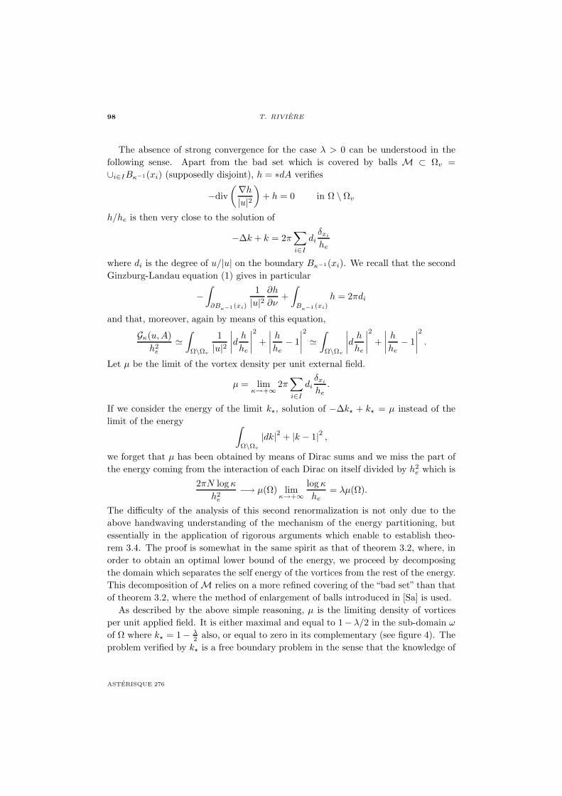
98 T. RIVIERE
The absence of strong convergence for the case λ > 0 can be understood in thefollowing sense. Apart from the bad set which is covered by balls M ⊂ Ωv =∪i∈IBκ−1(xi) (supposedly disjoint), h = ∗dA verifies
−div(∇h
|u|2
)+ h = 0 in Ω \ Ωv
h/he is then very close to the solution of
−∆k + k = 2π∑i∈I
diδxi
he
where di is the degree of u/|u| on the boundary Bκ−1(xi). We recall that the secondGinzburg-Landau equation (1) gives in particular
−∫
∂Bκ−1 (xi)
1|u|2
∂h
∂ν+∫
Bκ−1 (xi)
h = 2πdi
and that, moreover, again by means of this equation,
Gκ(u, A)h2
e
∫
Ω\Ωv
1|u|2
∣∣∣∣d h
he
∣∣∣∣2 +∣∣∣∣ hhe
− 1∣∣∣∣2 ∫
Ω\Ωv
∣∣∣∣d h
he
∣∣∣∣2 +∣∣∣∣ hhe
− 1∣∣∣∣2 .
Let µ be the limit of the vortex density per unit external field.
µ = limκ→+∞
2π∑i∈I
diδxi
he.
If we consider the energy of the limit k, solution of −∆k + k = µ instead of thelimit of the energy ∫
Ω\Ωv
|dk|2 + |k − 1|2 ,
we forget that µ has been obtained by means of Dirac sums and we miss the part ofthe energy coming from the interaction of each Dirac on itself divided by h2
e which is2πN log κ
h2e
−→ µ(Ω) limκ→+∞
log κ
he= λµ(Ω).
The difficulty of the analysis of this second renormalization is not only due to theabove handwaving understanding of the mechanism of the energy partitioning, butessentially in the application of rigorous arguments which enable to establish theo-rem 3.4. The proof is somewhat in the same spirit as that of theorem 3.2, where, inorder to obtain an optimal lower bound of the energy, we proceed by decomposingthe domain which separates the self energy of the vortices from the rest of the energy.This decomposition of M relies on a more refined covering of the “bad set” than thatof theorem 3.2, where the method of enlargement of balls introduced in [Sa] is used.
As described by the above simple reasoning, µ is the limiting density of vorticesper unit applied field. It is either maximal and equal to 1− λ/2 in the sub-domain ω
of Ω where k = 1− λ2 also, or equal to zero in its complementary (see figure 4). The
problem verified by k is a free boundary problem in the sense that the knowledge of
ASTERISQUE 276

(868) GINZBURG-LANDAU VORTICES 99
Ω
ω = supp µ
Figure 4. Free-boundary problem
ω determines k in a unique way. This is an obstacle-problem, now quite classical,considered in particular in [R]. It has been shown by A. Bonnet and R. Monneau in[BM] that ∂ω is regular for almost all the values of λ and that, whenever it is thecase, ω is determined by the existence of the solution (...) of the following problem.
(56)
⎧⎪⎪⎪⎪⎪⎪⎪⎪⎪⎪⎪⎨⎪⎪⎪⎪⎪⎪⎪⎪⎪⎪⎪⎩
−∆k + k = 0 in Ω \ ω
k = 1− λ
2in ω
∂k
∂ν= 0 on ∂ω
k = 1 on ∂Ω.
3.6. Conclusion
What about the Abrikosov lattices? It would be interesting, in the previous ap-proach, to place oneself at a scale 1/
√he -the minimal mean relative distance between
two vortices- and to try then to understand the limit κ → +∞. We can hope in thisasymptotic, to show the existence of an infinite renormalized energy on countable con-figurations of points of R2, which govern the set up of the vortices amongst themselvesand try to understand the fundamental states of this energy by restraining ourselves,in a first approach, to periodic lattices. The first difficulty of this analysis is to un-derstand the terms of lower order in the expansion of the energy (55). The first termonly gives the mean density of vortices and does not see their relative positions toO(1/
√he).
SOCIETE MATHEMATIQUE DE FRANCE 2002
100 T. RIVIERE
In his PhD thesis, M. Dutour [D] adopts a different approach which we shall notdevelop more extensively here since that would lead us beyond the scope of this talk.One places oneself on any flat torus T , which can be seen as a unit cell of a latticeof R2, and whose size and geometry are variables of the problem. On that cell T
which is considered occupied by only one vortex (one fixes a complex line bundle E
on T of Euler class equal to 1), one studies the minima of Gκ the Ginzburg-Landaufunctional under the action of an external uniform field he. When the external fieldincreases, the increase in the vortex density, in that model, gives rise to a decrease inthe size of the cell T , etc. M. Dutour thus gives a very complete description of thephase diagram (figure 1) namely in the vicinity of Hc2 , where he manages to showthe existence of exactly two solutions; the first with vortices (close to one another by κ−1) and the second in the normal state dA = he. He establishes whether eachof these solutions is minimizing or not with respect to he, and accounts for the largeprecision of the Abrikosov bifurcation from the critical value 1/2. The optimality ofsuch or such lattice is only partially discussed, but this approach seems to open a newdirection towards a rigorous understanding of the relative positions of the vortices inthe fundamental state (very far from the boundary which has disappeared from thismodel) and eventually of the energetically favorable nature of the Abrikosov triangularlattices.
REFERENCES
[Ab] A. Abrikosov – On the magnetic properties of superconductors of the secondtype, Soviet Phys. JETP 5, 1174-1182 (1957).
[Af] A. Aftalion – On the minimizers of the Ginzburg-Landau energy for highkappa: the one-dimensional case, European J. Appl. Math. 8, 331-345 (1997).
[AT] A. Aftalion and C. Troy – On the solutions of the one dimensionalGinzburg-Landau Equations, Preprint LMENS (1998).
[AB1] L. Almeida and F. Bethuel – Multiplicity results for the Ginzburg-Landauequation in presence of symmetries, Houston J. Math. 23, 733-764 (1997).
[AB2] L. Almeida and F. Bethuel – Topological methods for the Ginzburg-Landauequations, J. Math. Pures Appl. 77, 1-49 (1998).
[BBC] H. Berestycki, A. Bonnet and J. Chapman – A semi-elliptic systemarising in the theory of type-II superconductivity, Comm. Appl. Non-linearAnal. 1, 1-21 (1994).
[BC] M. S. Berger and Y. Y. Chen – Symmetric vortices for the Ginzburg-Landau equations of superconductivity and the nonlinear desingularizationphenomenon, Journal of Funct. Anal. 82, 259-295 (1989).
ASTERISQUE 276
(868) GINZBURG-LANDAU VORTICES 101
[BBH0] F. Bethuel, H. Brezis, and F. Helein – Asymptotics for the minimizationof a Ginzburg-Landau functional, Calc. Var. Partial Differ. Equ. 1, 2, 123-148(1993).
[BBH] F. Bethuel, H. Brezis and F. Helein – Ginzburg-Landau vortices,Birkhauser (1994).
[BR1] F. Bethuel and T. Riviere – Vortices for a variational problem relatedto supraconductivity, Ann. Inst. Henri Poincare, Anal. Non Lineaire 12, 3,243-303 (1995).
[BR2] F. Bethuel and T. Riviere – Vorticite dans les modeles de Ginzburg-Landau pour la supraconductivite, Seminaire EDP de l’Ecole Polytechnique,expose XVI (1994).
[Bog] B. Bogomol’nyi – Soviet J. Nucl. Phys. 24, 449 (1976).[BH1] C. Bolley and B. Helffer – Rigorous results on Ginzburg-Landau models
in a film submitted to an exterior parallel magnetic field I and II, Non LinearStud. 3, 1-29 and 121-152 (1996).
[BH2] C. Bolley and B. Helffer – The ginzburg-Landau equations in a semi-infinite superconducting film in the large κ limit, European J. Appl. Math. 8,347-367 (1997).
[BCM] A. Bonnet, J. Chapman and R. Monneau – Convergence of Meissnerminimizers of the Ginzburg-Landau energy of superconductivity as κ → +∞,preprint (1999).
[BM] A. Bonnet and R. Monneau – Existence of a smooth free-boundary in a su-perconductor with a Nash-Moser inverse function theorem argument, preprint(1999).
[BBM] J. Bourgain, H. Brezis and P. Mironescu – Lifting properties of Sobolevmaps, in preparation.
[BMR] H. Brezis, F. Merle and T. Riviere – Quantization effects for −∆u =u(1− |u|2) in R2, Arch. Rat. Mech. Analysis. 126, 123-145 (1994).
[DL] Q. Du and H. Lin – Ginzburg-Landau vortices: dynamics, pinning and hys-teresis, Siam J. Math. Anal. 28, 1265-1293 (1997).
[D] M. Dutour – Bifurcation vers l’etat d’Abrikosov et diagramme de phase,these de l’Universite Paris-Sud, Orsay (1999).
[dG] G. De Gennes – Superconductivity of Metal and Alloys, Benjamin, New-York and Amsterdam (1966).
[GS] S. Gueron and I. Shafrir – On a discrete variational problem involvinginteracting particles, to appear in SIAM J. Appl. Math. (1999).
[JT] A. Jaffe and C. Taubes – Vortices and Monopoles, Birkhauser (1980).[J] R. Jerrard – Lower bounds for generalized Ginzburg-Landau functionals,
SIAM J. Math. Anal. 30, 721-746 (1999).
SOCIETE MATHEMATIQUE DE FRANCE 2002

102 T. RIVIERE
[LL] H. Lin and C. Lin – Minimax solutions of the Ginzburg-Landau equations,Selecta Mathematica, New Series 3, 99-113 (1997).
[LR] H. Lin and T. Riviere – Complex Ginzburg-Landau equations and codi-mension 2 minimal surfaces, J.E.M.S. 1, 3 (1999).
[LR2] H. Lin and T. Riviere – A quantization property for static Ginzburg-Landau vortices, Comm. Pure and App. Math. (2000).
[Mi] P. Mironescu – Les minimiseurs locaux pour l’equation de Ginzburg-Landausont a symetrie radiale, C.R. Acad. Sci. Paris, Ser. 1, 323, 593-598 (1996).
[OS] N. Ovchinnikov and M. Sigal – The Ginzburg-Landau equation I. Staticvortices, Partial differential equations and their applications (Toronto, ON,1995), 199-220, CRM Proc. Lecture Notes 12, Amer. Math. Soc., Providence,RI (1997).
[PR] F. Pacard and T. Riviere – Linear and non-linear aspects of vortices,Birkhauser (2000).
[Qin] J. Qing – Renormalized energy for Ginzburg-Landau vortices on closed sur-faces, Math. Z. 225, 1-34 (1997).
[Ri1] T. Riviere – Asymptotic analysis for the Ginzburg-Landau equations, ETH-Zurich course, January 1997, Boll U.M.I. (1999).
[Ri2] T. Riviere – Line vortices in the U(1)−Higgs Model, COCV 1, 77-167(1995).
[Ri3] T. Riviere – Some progress towards Jaffe and Taubes Conjectures, preprint(1999).
[R] F. Rodrigues – Obstacle problems in mathematical physics, MathematicalStudies, North Holland (1987).
[SST] D. Saint-James, G. Sarma and J. Thomas – Type-II Superconductivity,Pergamon Press (1969).
[Sa] E. Sandier – Lower bounds for the energy of unit vector fields and applica-tions, J. Funct. Anal. 152, 379-403 (1998).
[SS1] E. Sandier and S. Serfaty – Global minimizers for the Ginzburg-Landaufunctional below the first critical magnetic field, to appear in Annales del’Inst. Henri Poincare, Analyse non-lineaire (1999).
[SS2] E. Sandier and S. Serfaty – A rigourous derivation of a free-boundaryproblem arising in superconductivity, Ann. Sci. Ec. Norm. Sup. 33 (2000),561-592.
[Se1] S. Serfaty – Etude mathematique de l’equation de Ginzburg-Landau de lasupraconductivite, These de l’Universite Paris-Sud, Orsay (1999).
[Se2] S. Serfaty – Local minimizers for the Ginzburg-Landau energy near criticalmagnetic field I and II, Comm. Contemporary Mathematics 1, n 2 et 3,213-254 (1999).
ASTERISQUE 276
(868) GINZBURG-LANDAU VORTICES 103
[Se3] S. Serfaty – Stable configurations in superconductivity: uniqueness, multi-plicity and vortex-nucleation, to appear in : Arch. Rat. Mech. Anal. (1999).
[St] M. Struwe – On the asymptotic behavior of minimizers of the Ginzburg-Landau model in 2 dimensions, J. Diff. Int. Equations 7 (1994), 1613-1624and Erratum in J. Diff. Int.
[Ti] M. Tinkham – Introduction to Superconductivity, 2nd edition, McGraw-Hill(1996).
[Uh] K. Uhlenbeck – Connections with Lp bounds on curvature, Comm. Math.Phys. 83, 31-42 (1982).
Tristan RIVIERE
Centre de MathematiquesEcole polytechniqueF-91128 Palaiseau CedexE-mail : [email protected]
SOCIETE MATHEMATIQUE DE FRANCE 2002


Seminaire BOURBAKI Novembre 199952e annee, 1999-2000, no 869, p. 105 a 135
PROGRES RECENTSSUR LA CONJECTURE DE BAUM–CONNES.CONTRIBUTION DE VINCENT LAFFORGUE
par Georges SKANDALIS
Cet expose fait de nouveau le point sur la conjecture de Baum-Connes apres celui dePierre Julg ([25]) qui rendait compte d’une avancee spectaculaire obtenue par Higsonet Kasparov ([19]). Une nouvelle barriere vient juste d’etre franchie par V. Lafforgue :celle de la propriete T de Kazhdan. Le but ici est d’exposer les diverses etapes dutravail de Lafforgue. En fin d’expose, nous donnerons quelques autres resultats enrelation avec la conjecture de Baum-Connes et celle de Novikov obtenus recemmentpar G. Yu ([51]), N. Higson ([18]) et quelques autres.
La conjecture de Baum-Connes predit la K-theorie de la C∗-algebre (reduite) d’ungroupe discret G et, plus generalement, d’un groupe localement compact, et memed’un groupoıde localement compact (par exemple de la C∗-algebre associee a unfeuilletage) etc. Cette conjecture a plusieurs consequences : l’injectivite du morphismede Baum-Connes a des implications geometriques importantes — la plus fameuse etantla conjecture de Novikov sur les « hautes signatures » ; sa surjectivite a des applica-tions fondamentales dans la theorie des C∗-algebres (e.g. une conjecture de Kadison,deja ancienne, sur les idempotents).
Malgre les efforts de plusieurs mathematiciens, une barriere subsistait pour lapreuve de cette conjecture : la propriete T de Kazhdan (cf. [32], [12]), qui empechecertaines idees de demonstration d’aboutir et rend fausses certaines generalisations :en effet, cette conjecture est alors fausse si la C∗-algebre pleine remplace la reduite(cf. [24], voir aussi [10]) ; la generalisation de cette conjecture au bifoncteur de Kas-parov (qui generalise la K-theorie) peut elle-meme etre fausse (cf. [44]). Au-dela decette barriere, les seuls cas connus avant le travail de Lafforgue etaient les groupesde Lie reels reductifs (A. Wassermann [50]) ou p-adiques (Baum-Higson-Plymen [6])utilisant la description complete de la C∗-algebre de ces groupes, mais aucun groupediscret infini possedant la propriete T n’avait pu etre obtenu.
Lafforgue etablit la conjecture de Baum-Connes pour beaucoup de groupes locale-ment compacts ayant la propriete T : tout groupe de Lie semi-simple reel ou reductifp-adique ET les sous-groupes discrets cocompacts des groupes de Lie de rang reel 1ou de SL3 d’un corps local.
SOCIETE MATHEMATIQUE DE FRANCE 2002
106 G. SKANDALIS
Dans tous ces cas, l’injectivite du morphisme de Baum-Connes etait connue (tra-vaux de Miscenko, Solovjev, Kasparov...). En fait, il y a un element note γ par Kas-parov dans l’anneau de representations (defini par Kasparov) KKG(C,C) dont ladifference avec 1, mesure la non surjectivite du morphisme de Baum-Connes. On doitmontrer que γ = 1 en tant qu’endomorphisme de la K-theorie de la C∗-algebre reduiteC∗
r (G) de G. Remarquons que, par la propriete T , γ lui-meme n’est pas egal a 1 dansl’anneau KKG(C,C) et meme dans l’anneau KK(C∗
r (G), C∗r (G)) (du moins si G est
un sous-groupe discret cocompact de Sp(n, 1) — cf. [44]).La demonstration de Lafforgue a trois etapes. La premiere est sa principale contri-
bution conceptuelle ; la seconde est — de loin — la plus difficile techniquement ; dansla troisieme, il utilise des travaux de Jolissaint dans le cas Sp(n, 1) et de Ramagge-Robertson-Steger dans le cas de SL3 d’un corps local non archimedien ; enfin, il adaptela methode de Ramagge-Robertson-Steger pour obtenir aussi le cas des sous-groupesdiscrets cocompacts de SL3(R) et SL3(C).
Plus explicitement :
1. Dans la premiere etape, Lafforgue construit un bifoncteur KKban(A, B) pourdes algebres de Banach, en remplacement de la theorie bivariante de Kasparov. Ils’agit la d’une construction nouvelle et tres interessante. Elle suit d’assez pres cellede Kasparov. Cependant, les C∗-modules hilbertiens qui sont a la base du travail deKasparov sont ici remplaces par des paires de modules banachiques en dualite (lesmodules hilbertiens des C∗-algebres sont en ce sens autoduaux). Malheureusement, leproduit de Kasparov ne se generalise pas directement a ce cadre. Cependant, Lafforgueparvient a etendre plusieurs constructions de Kasparov dans cette « KK-theorie ba-nachique » : il demontre qu’elle opere sur la K- theorie, construit une KK-theoriebanachique equivariante par un groupe localement compact, ainsi qu’un analogue del’homomorphisme de descente jG : KKG(A, B) → KK(A G, B G) de Kasparov.
2. Dans la deuxieme etape il etablit l’egalite γ = 1 dans sa KK-theorie banachiqueequivariante pour tout groupe localement compact agissant de facon continue, propreet isometrique sur :
– une variete riemannienne complete, connexe, simplement connexe a courburesectionnelle negative ou nulle (cette classe contient tous les groupes de Lie reels ettous leurs sous-groupes fermes) ;
– sur un immeuble affine (cette classe contient tous les groupes de Lie p-adiques ettous leurs sous-groupes fermes).C’est la partie la plus technique. Il construit une homotopie qui utilise :
– dans le cas reel des espaces de Sobolev de formes Lp sur des varietes de courburesectionnelle negative ;
– dans le cas p-adique une combinatoire assez elaboree (ainsi que des espaces p).A l’aide des parties 1 et 2, Lafforgue etablit la conjecture de Baum-Connes a valeurs
dans la sous-algebre L1(G) de C∗r (G) (ce qui prouve une conjecture de Bost), ainsi que
ASTERISQUE 276

(869) LA CONJECTURE DE BAUM-CONNES 107
toutes les completions de Cc(G) pour des « normes inconditionnelles » (dans le langagede Lafforgue) i.e. une norme d’algebre N satisfaisant N(f) ≤ N(g) si f, g ∈ Cc(G)satisfont, pour tout x ∈ G, |f(x)| ≤ |g(x)| (notons cependant que la norme de C∗
r
n’est malheureusement pas « inconditionnelle »).
3. Pour prouver la conjecture de Baum-Connes, il suffit de construire une « comple-tion inconditionnelle » de Cc(G), qui soit une sous-algebre A de C∗
r (G) avec la memeK-theorie que C∗
r (G). Pour cela, il suffit que A soit stable par calcul fonctionnelholomorphe dans C∗
r (G). Une telle sous-algebre A existe :
– si G est un groupe de Lie semi-simple, Lafforgue montre qu’une variante del’algebre de Harish-Chandra convient (cf. [36]) ;
– si G est un groupe hyperbolique e.g. un sous-groupe discret cocompact dansSp(n, 1) (travaux de Haagerup pour les groupes libres, de Jolissaint pour les sous-groupes cocompacts des groupes de Lie de rang 1, et de de la Harpe pour un groupehyperbolique quelconque [17]) ;
– si G est discret cocompact dans SL3 d’un corps local non archimedien (ce resultatest du a Ramagge, Robertson et Steger [41]) ;
– si G est discret cocompact dans SL3(R) ou SL3(C) : ce resultat est du a Laf-forgue [34].
Dans ces trois derniers cas, l’algebre A est donnee par des conditions de decroissancerapide au sens 2.
Nous commencerons cet expose par quelques rappels, notamment sur lesC∗-algebres de groupes et la theorie de Kasparov. Ensuite, nous rappellerons laconjecture de Baum-Connes et ses generalisations. Nous renvoyons a ce sujet al’excellent expose de Pierre Julg [25]. Les trois paragraphes suivants seront consacresaux trois etapes du travail de Lafforgue citees ci-dessus. Dans le dernier paragraphe,nous decrivons de tres recents resultats de Yu ([51]) et Higson ([18]) relies a laconjecture de Baum-Connes.
Ajout (mars 2000). — Depuis que cet expose a ete ecrit, des contre-exemples a laconjecture de Baum-Connes pour les feuilletages, ainsi que ses analogues pour les« structures a l’infini » ont ete donnes (cf. [20]). Ceux-ci sont bases sur des idees deM. Gromov (cf. [15]).
Je tiens a remercier Vincent Lafforgue pour de nombreuses explications sur sestravaux. Je le remercie aussi, ainsi que Saad Baaj, Jean Renault et Alain Valette,pour une lecture attentive de ce manuscrit. Un grand merci enfin a Alberto Arabiapour son aide amicale.
SOCIETE MATHEMATIQUE DE FRANCE 2002

108 G. SKANDALIS
1. RAPPELS ET NOTATIONS : C∗-ALGEBRES DE GROUPES,THEORIE DE KASPAROV
1.1. Algebres de Banach ; C∗-algebres
Toutes les algebres de Banach que nous considerons dans cet expose sont complexes.Si A est une algebre de Banach, on supposera toujours que sa norme verifie ‖ab‖ ≤‖a‖‖b‖, pour tout a, b ∈ A. On ne suppose pas en general que nos algebres de Banachpossedent un element unite. Si A est une algebre de Banach, on note A l’algebre deBanach unifere construite de la facon suivante : en tant qu’espace vectoriel A estisomorphe au produit A × C ; sa norme est donnee par ‖(a, λ)‖ = ‖a‖ + |λ| (poura ∈ A et λ ∈ C) et son produit est donne par (a, λ)(b, µ) = (ab + λb + µa, λµ) (poura, b ∈ A et λ, µ ∈ C). On identifie A avec son image dans A par l’homomorphismea → (a, 0) ; l’element (0, 1) est l’unite de A.
Un A-module banachique a droite (resp. a gauche) est un espace de Banach E munid’une action a droite (resp. a gauche) de A telle que, pour tout x ∈ E et tout a ∈ A,on ait ‖xa‖ ≤ ‖x‖‖a‖ (resp. ‖ax‖ ≤ ‖a‖‖x‖). Un A-module banachique a droite (resp.a gauche) est un A-module banachique a droite (resp. a gauche) : il suffit de poserx(a, λ) = xa + λx (resp. (a, λ)x = ax + λx) pour a ∈ A, x ∈ E, et λ ∈ C.
Rappelons qu’une inolution sur une algebre de Banach est une application anti-lineaire, antimultiplicative, involutive et isometrique notee x → x∗. Une algebre deBanach involutive est une algebre de Banach munie d’une involution.
Une C∗-algebre est une algebre de Banach involutive A telle que, pour tout x ∈ A,on ait ‖x∗x‖ = ‖x‖2. Si A est une C∗-algebre, l’algebre de Banach obtenue a partir deA en adjoignant une unite est involutive (on pose (a, λ)∗ = (a∗, λ)) ; ce n’est cependantpas une C∗-algebre. Il existe neanmoins une (unique) norme de C∗-algebre sur A.
1.2. C∗-algebres de groupes
Soit G un groupe localement compact. Notons dx une mesure de Haar a gauchesur G et Cc(G) l’algebre de convolution des fonctions continues a support compactsur G. Rappelons que la convolee f g de f, g ∈ Cc(G) est donnee par la formule
f g(x) =∫
G
f(y)g(y−1x) dy
pour tout x ∈ G.Par ailleurs, on definit une involution f → f∗ sur Cc(G) en posant f∗(x) =
∆(x−1)f(x−1) ou ∆ designe la fonction module sur G (telle que, pour tout f ∈ Cc(G),on ait∫
f(x−1) dx =∫
f(x)∆(x) dx ).Il y a plusieurs facons de completer Cc(G) en une algebre de Banach, c’est-a-dire
des normes sur Cc(G) telles que, pour tout f, g ∈ Cc(G) on ait ‖f g‖ ≤ ‖f‖‖g‖.Nous en utiliserons (au moins) 3 :
ASTERISQUE 276
(869) LA CONJECTURE DE BAUM-CONNES 109
1. La plus simple est de prendre la norme ‖ ‖1. On obtient l’algebre de BanachL1(G).
2. Une autre facon est de considerer Cc(G) comme operant sur L2(G) par convo-lution : pour f ∈ Cc(G), on note λ(f) l’application de L2(G) dans lui-meme donneepar g → λ(f)(g) = f g. On note ‖f‖r la norme d’operateur de λ(f) (dans L2(G)).Le complete de Cc(G) pour cette norme est une C∗-algebre appelee la C∗-algebrereduite de G et notee C∗
r (G). De facon equivalente, C∗r (G) s’identifie avec l’adherence
normique de λ(Cc(G)) dans l’algebre des operateurs de l’espace hilbertien L2(G). Onpeut remarquer que :
– pour f ∈ Cc(G), on a ‖λ(f)‖ ≤ ‖f‖1, donc la representation λ s’etend a L1(G),et que
– la representation λ est involutive : pour tout f ∈ Cc(G), on a λ(f∗) = λ(f)∗ ou,pour un operateur T d’un espace hilbertien, T ∗ designe l’adjoint de T .
3. Considerons toutes les representations involutives σ de Cc(G) dans un espacehilbertien Hσ telles que, pour tout f ∈ Cc(G) , on ait ‖σ(f)‖ ≤ ‖f‖1. Posons ‖f‖p =supσ ‖σ(f)‖. On obtient encore une norme ; le complete de Cc(G) pour cette normeest une C∗-algebre notee C∗(G) et appelee la C∗-algebre de G ou la C∗-algebre pleinede G. L’identite de Cc(G) se prolonge evidemment en un morphisme C∗(G) → C∗
r (G).Ce morphisme est toujours surjectif. Il est injectif si et seulement si le groupe G estmoyennable.
1.3. Produits croises
Soient G un groupe localement compact et A une algebre de Banach. Une actionde G dans A est un homomorphisme α de G dans le groupe des automorphismesisometriques de A, tel que, pour tout a ∈ A, l’application x → (α(x))(a) soit continue.Le plus souvent, pour x ∈ G et a ∈ A l’element (α(x))(a) ∈ A s’ecrira juste x.a.
Soit α une action d’un groupe G dans une algebre de Banach A. L’espace de BanachL1(G; A) est muni du produit de convolution donne par la formule
f g(x) =∫
G
f(y) y.(g(y−1x)) dy
pour tout f, g ∈ Cc(G; A) ⊂ L1(G; A) et x ∈ G.
Si A est une C∗-algebre et α respecte l’involution (x.(a∗) = (x.a)∗ pour tout a ∈ A
et tout x ∈ G), alors l’algebre de Banach L1(G; A) est naturellement munie d’uneinvolution par la formule (f∗)(x) = ∆(x−1)x.(f(x−1))∗. Generalisant la constructionde C∗
r (G) et C∗(G), on obtient par completion de L1(G; A) deux C∗-algebres A r G
et A G appelees respectivement produit croise reduit et plein de A par G.
SOCIETE MATHEMATIQUE DE FRANCE 2002
110 G. SKANDALIS
1.4. Theorie de Kasparov
Nous rappelons ici, tres sommairement, certaines constructions et proprietes dubifoncteur de Kasparov (cf. [28], [29] ; voir aussi les exposes de T. Fack [13] et P. Julg[25]).
1.4.a. Modules hilbertiens
Les A-modules hilbertiens sont les espaces hilbertiens avec les scalaires remplacespar A.
Rappelons qu’un element a d’une C∗-algebre A est appele positif s’il est de la formex∗x (x ∈ A). L’ensemble A+ des elements positifs joue le role de R+ dans C.
On appelle A-module prehilbertien sur A un A-module a droite E muni d’un « pro-duit scalaire » i.e. d’une application sesquilineaire E × E ' (x, y) → 〈x, y〉 ∈ A, telleque, pour tout x ∈ E, l’application y → 〈x, y〉 est A-lineaire (a droite), satisfaisant〈x, y〉∗ = 〈y, x〉 et 〈x, x〉 ∈ A+ pour tout x ∈ E.
Si E est un A-module prehilbertien, l’application x →√‖〈x, x〉‖ est une semi-
norme sur E. Si E est separe et complet pour cette norme on dit que c’est un A-modulehilbertien.
1.4.b. Operateurs ; operateurs compacts
Soient E, F des A-modules hilbertiens. L’ensemble des operateurs de E dans F
que nous considerons sont les operateurs T : E → F possedant un adjoint, i.e. uneapplication T ∗ : F → E satisfaisant 〈T (x), y〉 = 〈x, T ∗(y)〉 pour tout x ∈ E et y ∈ F .Un tel operateur est automatiquement lineaire, A- lineaire et continu. L’ensemble desoperateurs de E dans F est note L(E, F ). L’ensemble L(E) = L(E, E), muni de lanorme des applications lineaires continues, est une C∗-algebre.
En particulier, pour tout x ∈ E et y ∈ F , posons θy,x : z → y〈x, z〉. C’est unelement de L(E, F ) et θ∗y,x = θx,y. On note K(E, F ) le sous-espace vectoriel fermede L(E, F ) engendre par les θy,x. L’ensemble K(E) = K(E, E) est un ideal bilatereferme dans L(E).
Il sera utile de considerer les modules hilbertiens Z/2Z-gradues, c’est-a-dire lesmodules hilbertiens E = E(0) ⊕ E(1), ou E(0) et E(1) sont orthogonaux pour 〈 , 〉.Pour i ∈ Z/2Z, on note L(E)(i) l’ensemble des T ∈ L(E) tels que T (x) ∈ E(i+j) pourtout j ∈ Z/2Z et tout x ∈ E(j).
1.4.c. Cycles en KK-theorie
Soient A et B des C∗-algebres. Le groupe de Kasparov KK(A, B) est donne par descycles et une relation d’equivalence sur ces cycles. Un cycle est un triplet (E, π, F ) ouE est un B-module hilbertien Z/2Z-gradue, π : A→ L(E)(0) est un homomorphismeinvolutif (tel que π(a∗) = π(a)∗) et F ∈ L(E)(1) est tel que F = F ∗ et, pour touta ∈ A, les operateurs Fπ(a)− π(a)F et (F 2 − 1)π(a) sont dans K(E).
La somme des cycles (E, π, F ) et (E′, π′, F ′) est, avec des notations evidentes,(E ⊕ E′, π ⊕ π′, F ⊕ F ′).
ASTERISQUE 276
(869) LA CONJECTURE DE BAUM-CONNES 111
1.4.d. Homotopie
Notons B[0, 1] la C∗-algebre des applications continues de l’intervalle [0, 1] dans B.Un cycle pour KK(A, B[0, 1]) est une famille (Et, πt, Ft) de cycles pour KK(A, B) :c’est par definition une homotopie entre (E0, π0, F0) et (E1, π1, F1).
Le groupe de Kasparov KK(A, B) est l’ensemble des classes d’homotopie de cycles.Ce groupe est fonctoriel en A et en B : pour tout A on a un foncteur covariantB → KK(A, B) et pour tout B on a un foncteur contravariant A → KK(A, B).
1.4.e. Produit de Kasparov
Kasparov a defini un produit KK(A, B) × KK(B, C) → KK(A, C) (ou A, B, C
sont des C∗-algebres) qui est bilineaire, naturel et associatif. Le fait que ce produitsoit hautement non trivial donne toute sa force a la theorie. Muni de ce produit,KK(A, A) est un anneau. Son element unite note 1A est represente par (A, π, 0) ouA est gradue par A(0) = A et π(a)b = ab.
1.4.f. Action sur la K-theorie
Le groupe KK(C, A) a ete identifie par Kasparov avec le groupe de K-theorieK0(A). Le produit de Kasparov donne en particulier un morphisme de groupesKK(A, B)→ Hom(K0(A), K0(B)).
1.4.g. Le cas equivariant
On suppose a present qu’un groupe localement compact G opere sur les C∗-algebresA et B. On definit un groupe KKG(A, B) en demandant que G opere aussi surles cycles : un cycle pour KKG(A, B) est encore donne par un triple (E, π, F ), quiest un cycle pour KK(A, B), tel que G opere dans E de facon continue (i.e. pourtout x ∈ E l’application g → g.x est continue) ; on suppose de plus que, pour toutx, y ∈ E , a ∈ A , b ∈ B et g ∈ G, on a
g.(xb) = (g.x)(g.b) , 〈g.x, g.y〉 = g.(〈x, y〉) , g.(π(a)(x)) = π(g.a)(g.x) ;
enfin, pour tout a ∈ A et tout g ∈ G on a π(a)(g.F − F ) ∈ K(E) et g → π(a)(g.F )est continue en norme — ou g.F est donne par (g.F )(x) = g.(F (g−1.x)). Le groupeKKG(A, B) est l’ensemble des classes d’homotopie de cycles. Toutes les proprietes segeneralisent au cas equivariant ; en particulier, le produit de Kasparov se generalise ace cadre.
Remarque. — Soient G un groupe discret et (H, π, F ) un cycle pour KKG(A,C).L’action de G dans H et la representation π de A donnent une representation duproduit croise A G dans H . On en deduit que KKG(A,C) = KK(A G,C). Plusgeneralement si l’action de G dans B est triviale KKG(A, B) = KK(A G, B).
SOCIETE MATHEMATIQUE DE FRANCE 2002

112 G. SKANDALIS
1.4.h. Le morphisme jG
Si (E, π, F ) est un cycle pour KKG(A, B), on peut former le produit croise E r G
qui est un B r G-module hilbertien. On obtient aussi une representation naturelleπ : A r G → L(E r G) ; de plus, on associe a F un operateur F ∈ L(E r G).Le triplet (E r G, π, F ) est un cycle pour KK(A r G, B r G). On obtient ainsiun homomorphisme jr
G : KKG(A, B) → KK(A r G, B r G), compatible avec lesproduits de Kasparov.
On construit de meme un homomorphisme pour les produits croises pleins jG :KKG(A, B) → KK(A G, B G).
2. LA CONJECTURE DE BAUM-CONNES
La conjecture de Baum-Connes (cf. [5]) predit la K-theorie de C∗r (G).
Si G est un groupe de Lie connexe semisimple, elle predit que l’induction de Diracest un isomorphisme de la K-theorie de C∗(K), i.e. l’anneau des representations deK (1) — ou K est un sous-groupe compact maximal de G, sur celle de C∗
r (G).Si G est un groupe discret sans torsion, la conjecture predit que la K-theorie de
C∗r (G) est decrite par les G-indices sur des revetements M de groupe G d’une variete
compacte M (au sens de [3]).Pour l’enoncer correctement dans le cas general, nous aurons besoin de revenir sur
la notion d’espace classifiant pour un groupe.
2.1. Espaces classifiants
Soit G un groupe discret. L’espace classifiant BG est un espace muni d’un fibreprincipal ξ0 de fibre G. De plus, pour tout espace topologique X (2) et tout fibreprincipal ξ de fibre G, il existe une application continue f : X → BG, unique ahomotopie pres, telle que ξ soit isomorphe a f∗(ξ0). Ces proprietes determinent BG
a equivalence d’homotopie pres.Le groupe G opere sur l’espace total du fibre ξ0 — traditionnellement note EG
et BG est le quotient EG/G par l’action de G. L’espace EG et l’espace BG sont engeneral construits comme complexes cellulaires infinis. On peut cependant les supposerlocalement compacts (a l’aide d’une construction de telescope infini).
L’action de G sur EG est libre et propre(3). De plus, supposons que G opere li-brement et proprement sur un espace localement compact X . En considerant le fi-bre principal sur X/G, on deduit qu’il existe une application continue G-equivariante
(1)a des problemes mineurs de « K-orientation » pres.(2)On suppose X suffisamment regulier e.g. localement compact σ-compact, ou un complexe cellu-
laire.(3)Autrement dit, l’application (x, g) → (x, gx) est injective et propre de X × G dans X × X.
ASTERISQUE 276

(869) LA CONJECTURE DE BAUM-CONNES 113
g : X → EG, unique a homotopie G-equivariante pres. En ce sens, EG est un G-espacelibre et propre final dans cette categorie.
La conjecture de Baum-Connes utilise un G-espace propre final dans la categoriedes G-espaces propres. Un tel espace existe et est unique a G-homotopie pres (cf. [5],[31]). On le note EG. La construction de cet espace est en fait plus simple que cellede EG :
– un modele pour EG est l’ensemble des mesures de probabilite sur G ;– un modele localement compact pour EG est l’ensemble des mesures positives sur
G de masse totale dans ] 12 , 1], muni de la topologie de dualite avec l’algebre C0(G)des fonctions continues nulles a l’infini sur G ;
– si G est compact, on peut prendre pour EG un espace a un point !– si G est un groupe de Lie reel connexe, on peut prendre EG = G/K ou K est
un sous-groupe compact maximal ;– si G est un groupe de Lie reductif p-adique, on prendra pour EG la realisation
geometrique de l’immeuble affine associe ;– si G est discret, une presentation de EG via un complexe simplicial localement
fini rend possible l’utilisation d’arguments de type Mayer-Vietoris.
2.2. Le groupe de K-theorie topologique de Baum-Connes
Le groupe de K-theorie topologique K0,top(G), defini d’abord dans certains casparticuliers (groupes discrets, groupes de Lie, feuilletages... - cf. [4]), n’a ete biencompris en general que recemment (cf. [5], [47]) :
Soit G un groupe localement compact. Le groupe de K-theorie topologique est
K0,top(G) = lim→
KKG(C0(Y ),C) ,
ou la limite inductive est prise sur les parties fermees G-invariantes Y de EG tellesque Y/G soit compact(4).
Remarque. — Supposons que le groupe G soit discret. Dans ce cas, K0,top(G) =lim→
KK(C0(Y ) G,C) (voir remarque en 1.4.g).
Si de plus G est sans torsion, toute action propre de G est libre. Alors, la C∗-algebreC0(Y )G est equivalente au sens de Morita a C(Y/G) (en fait si G est infini, C0(Y )G est isomorphe a C(Y/G) ⊗ K, ou K designe l’algebre des operateurs compactssur un espace hilbertien). Comme la KK-theorie est invariante par equivalence deMorita, on en deduit que K0,top(G) = lim
→KK(C(X),C) la limite inductive etant
prise sur les parties compactes X de BG ; en d’autres termes, K0,top(G) est K0,c(BG),la K- homologie a support compact de BG.
(4)A une action continue a gauche de G sur un espace localement compact Y , correspond une action
de G sur la C∗-algebre C0(Y ) par la formule (g.f)(y) = f(g−1y), pour g ∈ G, f ∈ C0(Y ), y ∈ Y .
SOCIETE MATHEMATIQUE DE FRANCE 2002
114 G. SKANDALIS
2.3. L’homomorphisme de Baum-Connes
Soit Y un espace topologique localement compact muni d’une action propre de G ;on suppose de plus que Y/G est compact.
Si l’action de G est de plus libre, l’equivalence de Morita entre C0(Y ) G etC(Y/G) est donnee par un C0(Y ) G-module hilbertien canonique E, tel que K(E)soit isomorphe a C(Y/G) et qui est plein, c’est-a-dire que le sous-espace vectoriel fermede C0(Y ) G engendre par les produits scalaires 〈x, y〉 , x, y ∈ E est C0(Y ) G.
Si l’action est propre sans etre libre, on fait exactement la meme construction. Laseule chose qui change est que le C0(Y )G-module hilbertien canonique E n’est plusplein. Cependant, K(E) est encore egal a C(Y/G) ; en particulier, comme K(E) estunifere, (E, π, 0) definit un element ΛY de KK(C, C0(Y ) G).
Une facon equivalente plus elementaire de definir ΛY est la suivante : comme l’ac-tion de G dans Y est propre a quotient compact, il existe une fonction continue,positive, a support compact c : Y → R telle que, pour tout y ∈ Y ,
∫G c(gy) dg =
1. On note p ∈ Cc(Y × G) ⊂ Cc(G; C0(Y )) ⊂ C0(Y ) G la fonction (y, g) →∆(g)−1/2c(y)1/2c(g−1y)1/2. C’est un projecteur dans C0(Y ) G (i.e. p = p2 = p∗) ; ildefinit donc un element de K0(C0(Y ) G) = KK(C, C0(Y ) G).
La classe de p ne depend pas de la fonction c. En fait, le module p(C0(Y ) G) estisomorphe a E, ce qui fait le lien avec l’autre definition.
Soit maintenant x ∈ K0,top(G) ; il est represente par une partie Y ⊂ EG fermeeG-invariante telle que Y/G soit compact et un y ∈ KKG(C0(Y ),C). L’element µG(x)est le produit de Kasparov de ΛY ∈ KK(C, C0(Y ) G) et de jG(y) ∈ KK(C0(Y ) G, C∗(G)).
On verifie que cette construction passe a la limite inductive et qu’on obtient ainsiun homomorphisme µG : K0,top(G) → K0(C∗(G)). L’homomorphisme de Baum-Connes, ou homomorphisme d’assemblage en K-theorie est l’homomorphisme µG,r :K0,top(G) → K0(C∗
r (G)) obtenu par composition de µG avec l’homomorphisme deK-theorie associe a l’homorphisme de C∗-algebres λ : C∗(G) → C∗
r (G).
Conjecture de Baum-Connes. — L’homomorphisme µG,r est un isomorphisme.
2.4. Lien avec la conjecture de Novikov
Soit M une variete lisse compacte orientee. Notons Γ son groupe fondamental, M
son revetement universel. L’operateur de signature de M peut etre considere commeun operateur Γ-invariant sur M ; il definit ainsi un element de K-homologie equiva-riante KKΓ(C0(M),C), donc de K0,top(Γ) (comme l’action de Γ sur M est propre).
La conjecture de Novikov peut s’enoncer de la facon suivante : l’element deK0,top(Γ) associe a l’operateur de signature de M est rationnellement invariant parhomotopie. Autrement dit, si f : M → N est une equivalence d’homotopie entrevarietes lisses compactes orientees, la difference entre les elements de K0,top(Γ)associes aux operateurs de signature de M et de N est de torsion.
ASTERISQUE 276
(869) LA CONJECTURE DE BAUM-CONNES 115
Miscenko a demontre que l’image par la fleche de Baum-Connes µΓ de cet elementest invariant par homotopie (cf. [39]). Donc l’injectivite rationnelle de l’homomor-phisme de Baum-Connes implique la conjecture de Novikov.
Pour plus de details sur ce sujet, on peut voir aussi les exposes [13], [45].
2.5. Generalisations et variantes
Conjecture de Baum-Connes a coefficients
Soient G un groupe localement compact et A une C∗-algebre munie d’une ac-tion de G. On construit de meme un groupe de K-theorie topologique a coeffi-cients K0,top(G; A) = lim
→KKG(C0(Y ), A) et des homomorphismes de Baum-Connes
µAG : K0,top(G; A) → K0(A G) et µA
G,r : K0,top(G; A) → K0(A r G). On conjecturealors que µA
G,r est un isomorphisme.
Conjecture de Baum-Connes pour les groupoıdes
Soit G un groupoıde localement compact. On peut encore (cf. [42]) lui associer uneC∗-algebre et une C∗-algebre reduite (c’est de cette maniere que Connes construit laC∗-algebre d’un feuilletage — cf. [9]). A l’aide d’une generalisation aux groupoıdes dela K-theorie equivariante due a Le Gall (cf. [38]), on peut encore definir la K-theorietopologique et construire l’homomorphisme de Baum-Connes (cf. [4], [47]). On peut deplus definir un homomorphisme de Baum-Connes pour un groupoıde G a coefficientsdans une G-algebre.
Conjecture de Baum-Connes a valeurs dans L1 (due a J.-B. Bost).
En regardant d’un peu plus pres la construction de l’homomorphisme de Baum-Connes, on se rend compte que l’on peut construire en fait un homomorphisme µG,L1 :K0,top(G) → K0(L1(G)) et tel que µG est la composee de µG,L1 avec l’homomorphismede K-theorie associe a l’homomorphisme L1(G) → C∗(G). C’est en fait V. Lafforguequi, grace a sa KK-theorie banachique, a defini proprement l’homomorphisme µG,L1 .
2.6. Le point sur la conjecture
– La conjecture de Baum-Connes a coefficients dans n’importe quelle C∗-algebreest connue pour tous les groupes (ou groupoıdes) localement compacts moyennableset, plus generalement, ceux operant proprement par isometries affines sur un espacehilbertien ([19] — cf. [48] pour le cas des groupoıdes — voir a ce sujet l’expose de P.Julg [25]).
Par ailleurs, Oyono ([40]) et Chabert ([8]) ont demontre des resultats de stabilitede la conjecture a coefficients par certaines operations sur les groupes.
SOCIETE MATHEMATIQUE DE FRANCE 2002

116 G. SKANDALIS
– L’injectivite de l’homomorphisme de Baum-Connes (a coefficients) est de plusconnue
a) pour un groupe operant proprement par isometries sur une variete riemanniennecomplete a courbure sectionnelle negative ou nulle ([29]), et en particulier pour unsous-groupe ferme d’un groupe de Lie reel ;
b) pour un groupe operant proprement par isometries sur un immeuble affine et enparticulier pour un sous-groupe ferme d’un groupe de Lie p-adique ([30]) ;
c) pour un groupe operant proprement par isometries sur un espace metrique discretayant un « bon » comportement a l’infini (faiblement geodesique, a geometrie borneeet « bolique »— [31]) ;
d) pour un groupe admettant une action moyennable sur un espace compact ([18]).
– Lafforgue demontre la conjecture de Baum-Connes :e) pour tout groupe de Lie semi-simple reel ou p-adique. Ce resultat etait connu
dans le cas des groupes de Lie reels lineaires connexes reductifs (cf. [50]) et les groupesGLn p-adiques (cf. [6]) ;
f) pour les sous-groupes discrets cocompacts des groupes de Lie de rang reel 1 ou deSL3(K) — avec K = R, C, Qp. Dans ce cas on peut aussi admettre des coefficientsdans une algebre C(X), ou X est une variete riemannienne compacte munie d’uneaction isometrique de G. Dans le cas de rang 1, on n’a pas besoin de supposer quel’action de G dans X est isometrique.
C’est le resultat f) le plus spectaculaire de son travail, car il franchit la barriere dela propriete T pour un groupe discret, pour lequel il n’y a donc aucune descriptionpossible de C∗
r (G).
2.7. L’element γ de Kasparov
Dans tous les cas cites ci-dessus ou l’on connaıt l’injectivite de l’homomorphismeµG, on a en fait construit un homomorphsime inverse. Dans les cas a), b) et c) ci-dessus on sait decrire l’image de µG : on construit (cf. [29] dans le cas a), [26] dansle cas b), [31] dans le cas c)) un element γ ∈ KKG(C,C), qui est idempotent pour leproduit de Kasparov et satisfait :L’image de µG,r coıncide avec celle de l’endomorphisme idempotent de K0(C∗
r (G))associe a jr
G(γ) ∈ KK(C∗r (G), C∗
r (G)).En d’autres termes, la conjecture de Baum-Connes se ramene a la formulation
suivante : l’endomorphisme de K0(C∗r (G)) associe a jr
G(γ) est l’identite.
2.8. L’obstruction de la propriete T de Kazhdan
Rappelons (cf. [12]) qu’un groupe localement compact G possede la propriete T sila representation triviale est isolee dans son dual. Du point de vue des C∗-algebres,cela signifie qu’il existe un projecteur p ∈ C∗(G) tel que, pour toute representation π
de C∗(G) dans un espace hilbertien, π(p) soit le projecteur orthogonal sur les vecteursinvariants par G.
ASTERISQUE 276

(869) LA CONJECTURE DE BAUM-CONNES 117
Soit G un groupe localement compact non compact possedant la propriete T . No-tons λ : C∗(G) → C∗
r (G) l’homomorphisme canonique. Comme la representationreguliere de G ne possede pas de vecteurs G-invariants (car G n’est pas compact), ona λ(p) = 0. Or la classe de p est un element non trivial de la K-theorie de C∗(G),puisque son image par la representation triviale ε : C∗(G) → C n’est pas nulle dansK0(C) = Z. Il s’ensuit que λ n’induit pas un isomorphisme en K-theorie, donc que µG
et µG,r ne sont pas tous deux bijectifs. Une demonstration eventuelle de la conjecturede Baum-Connes doit donc necessairement distinguer entre C∗(G) et C∗
r (G).Supposons de plus que G est un groupe comme dans a), b) ou c) ci-dessus. En par-
ticulier, il possede un element γ. Par ce qui precede, l’endomorphisme de K0(C∗(G))associe a jG(γ) s’annule sur la classe de p ; il en resulte que γ = 1.
Par ailleurs, l’element γ est represente par un couple (H, F ) ou la representationde G dans l’espace hilbertien H est un sous-multiple de la reguliere ; comme la repre-sentation triviale est isolee, il est de toute facon impossible d’esperer une homotopieentre γ et 1.
3. KK -THEORIE BANACHIQUE
On a vu qu’en presence de la propriete T , il n’est pas possible de faire une homotopiede γ a 1 dans KKG(C,C).
Cependant, la representation triviale est isolee parmi les representations unitairesde G, c’est-a-dire des representations dans des espaces hilbertiens ; elle ne l’est pas dansles representations banachiques. Par exemple la famille des representations naturellesde G dans Lp(G) contient faiblement, quand p tend vers +∞, la representation triviale.
Il est donc possible d’esperer construire une homotopie entre γ et 1 si on s’autorisedes representations banachiques.
Lafforgue est ainsi amene a construire une KK-theorie, ou les espaces hilbertienssont remplaces par des espaces de Banach - et donc les C∗-algebres par des algebresde Banach. C’est la KK-theorie banachique.
3.1. B-paires
Contrairement aux espaces hilbertiens, les espaces de Banach ne sont pas auto-duaux. Pour cette raison, Lafforgue remplace les modules hilbertiens par des pairesde modules banachiques en dualite.
Soit B une algebre de Banach. Une B-paire est un couple de modules banachiquesen dualite. Autrement dit, une B-paire (E<, E>) est la donnee d’un B-module bana-chique a gauche (resp. a droite) E< (resp. E>) et d’une application 〈 , 〉 : E<×E> →B satisfaisant : ∀x ∈ E>, ξ ∈ E<, l’application η → 〈η, x〉 (resp. y → 〈ξ, y〉) estC-lineaire, B-lineaire a gauche (resp. a droite) et ‖〈ξ, x〉‖ ≤ ‖ξ‖‖x‖.
SOCIETE MATHEMATIQUE DE FRANCE 2002

118 G. SKANDALIS
Soient E = (E<, E>) et F = (F<, F>) des B-paires. Un morphisme de B-pairesde E dans F est un couple f = (f<, f>) ou f< : F< → E< (resp. f> : E> →F>) est une application C-lineaire, B- lineaire a gauche (resp. a droite), continueet satisfait : ∀x ∈ E>, η ∈ F<, on a 〈η, f>(x)〉 = 〈f<(η), x〉. On note L(E, F )l’espace de Banach des morphismes de B-paires de E dans F (muni de la norme(f<, f>) → sup(‖f<‖, ‖f>‖)).
Si E, F, G sont des B-paires, f ∈ L(E, F ) et g ∈ L(F, G) on definit gf ∈ L(E, F ) enposant (gf)> = g> f> et (gf)< = f<g<. Munie de ces operations L(E) = L(E, E)est une algebre de Banach.
Soient y ∈ F> et ξ ∈ E<. On note θy,ξ ∈ L(E, F ) (ou |y〉〈ξ|) le morphisme donnepar le couple d’applications F< ' η → 〈η, y〉ξ ∈ E< et E> ' x → y〈ξ, x〉 ∈ F>. Onnote K(E, F ) le sous-espace vectoriel ferme de L(E, F ) engendre par les morphismesθy,ξ.
3.2. Definition de la KK -theorie banachique
Soient A et B des algebres de Banach. Un cycle pour KKban(A, B) est encoreun triplet (E, π, f) ou E est une B-paire Z/2Z-graduee, π : A → L(E)(0) est unhomomorphisme et f ∈ L(E)(1) est tel que, pour tout a ∈ A, les morphismes fπ(a)−π(a)f et (f2 − 1)π(a) sont dans K(E).
La somme des cycles et l’homotopie sont definies comme dans le cas des moduleshilbertiens. Il est facile de voir que l’ensemble des classes d’homotopie de cycles (munide l’addition des cycles) est un groupe abelien.
Le groupe KKban(A, B) est l’ensemble des classes d’homotopie de cycles.La fonctorialite en A ne pose pas de probleme. Soit ϕ : B1 → B2 un homomor-
phisme d’algebres de Banach. Notons encore ϕ : B1 → B2 son extension unitale.Soit E1 une B1-paire. Considerons-la comme une B1 paire. On definit une B2-paireE2 = ϕ∗(E1) qui est le quotient du produit tensoriel E1⊗π B2 par le sous-espace fermeengendre par xb1 ⊗ b2 − x ⊗ ϕ(b1)b2 avec x ∈ E1, b1 ∈ B1 et b2 ∈ B2. On construitde plus un homomorphisme ϕ∗ : f → (f ⊗ 1) de L(E1) dans L(E2) qui envoie K(E1)dans K(E2). On en deduit un homomorphisme ϕ∗ : KKban(A, B1)→ KKban(A, B2).
3.3. Le cas equivariant
On suppose a present qu’un groupe localement compact G opere sur les algebres A
et B. On definit le groupe KKbanG (A, B) exactement de la meme facon que le groupe
de Kasparov correspondant.Si A et B sont des C∗-algebres, on a evidemment un homomorphisme naturel
KKG(A, B) → KKbanG (A, B).
Dans le paragraphe suivant, on esquissera le principal resultat technique de Laf-forgue montrant (presque) que l’image de γ est egale a celle de 1 dans KKban
G (C,C).
ASTERISQUE 276

(869) LA CONJECTURE DE BAUM-CONNES 119
Pour en deduire la conjecture de Baum-Connes, il reste a construire les equivalentsen KK-theorie banachique
– du morphisme jG : KKG(C,C) → KK(C∗r (G), C∗
r (G)),– de l’action de la KK-theorie sur la K-theorie, autrement dit un homomorphisme
KKban(A, B) → Hom(K0(A), K0(B)).
3.4. Action sur la K -theorie
Rappelons que si A est une algebre de Banach unifere, le groupe K0(A) est le groupede Grothendieck du monoıde des classes d’isomorphisme de A-modules projectifs detype fini. Un tel module est isomorphe a un pAn ou p ∈Mn(A) est un idempotent.
Remarquons que KKban(Mn(A), B) est isomorphe a KKban(A, B). Par ailleurs,tout idempotent p ∈ A determine un homomorphisme ip : λ → λp de C → A.De ces faits, on deduit une application bilineaire ϕ : (p, x) → (ip)∗(x) de K0(A) ×KKban(A, B) dans KKban(C, B).
Cet homomorphisme subsiste si A n’est plus supposee unifere.Lafforgue demontre de plus que, comme dans le cas de la theorie de Kasparov, l’ap-
plication naturelle (x → ϕ(x, 1A)) de K0(A) dans KKban(C, A) est un isomorphisme.On en deduit donc que la KK-theorie banachique opere encore sur la K-theorie.
3.5. Completions « inconditionnelles » et le morphisme jG
La construction de l’homomorphisme jrG : KKG(A, B) → KK(A r G, B r G)
n’est malheureusement pas possible telle quelle : pour cela, il faudrait un analoguedu produit croise pour les algebres de Banach, qui pour une C∗-algebre donnerait leproduit croise reduit.
Cependant, on peut construire dans le cadre des algebres de Banach le produitcroise L1(G; A). On en deduit un homomorphisme
jL1
G : KKbanG (A, B) → KKban(L1(G; A), L1(G; B)).
A l’aide de cet homomorphisme jL1
G , l’egalite γ = 1 dans KKbanG (C,C) implique
la conjecture de Baum-Connes dans L1(G). Pour conclure, il faudrait savoir que l’in-clusion L1(G) → C∗
r (G) induit un isomorphisme en K-theorie (la surjectivite suffit).Cependant, on n’a pas encore d’outil permettant de demontrer cet isomorphisme (cf.la discussion dans [7] ou cet isomorphisme est etabli dans quelques cas).
Ici intervient une tres jolie et simple idee de Lafforgue : celle de « completioninconditionnelle » : on remarque que pour certaines normes d’algebre sur Cc(G), engeneral plus petites que la norme L1, on peut quand meme former le produit croisebanachique :
Definition 1. — Une norme N d’algebre sur Cc(G) sera dite une norme incondi-tionnelle si, pour tout f, g ∈ Cc(G), on a |f(x)| ≤ |g(x)|, ∀x ∈ G ⇒ N(f) ≤ N(g).
SOCIETE MATHEMATIQUE DE FRANCE 2002
120 G. SKANDALIS
On peut construire des produits croises relatifs a toute norme inconditionnelle.Soient en effet G un groupe localement compact, N une norme inconditionnelle surCc(G) et A une algebre de Banach munie d’une action isometrique de G. MunissonsCc(G; A) du produit de convolution tordu par l’action de G dans A (voir 1.3).
Notons pN : Cc(G; A) → R+ l’application qui a f associe N(ϕ) ou ϕ est l’applica-tion x → ‖f(x)‖ de G→ R. L’application pN est une norme d’algebre sur Cc(G; A).
Notons A N G le complete de Cc(G; A) pour la norme pN . Si E est un espace deBanach muni d’une action isometrique de G, on peut de meme construire l’espace deBanach E N G. Si (E<, E>) est une B-paire, alors (E< N G, E> N G) est uneB N G-paire.
On obtient un homomorphisme jNG : KKban
G (A, B) → KKban(A N G, B N G).
Soit G un groupe dans les cas a), b) ou c) de 2.6. Pour montrer la conjecture deBaum-Connes pour G, il suffit donc de
1. Demontrer que γ = 1 dans KKbanG (C,C).
2. Construire une completion inconditionnelle de Cc(G) qui a la meme K-theorieque C∗
r (G).
3.6. Representations non isometriques de G
En fait, l’homotopie entre γ et 1 n’aura pas lieu dans le groupe KKbanG (C,C), mais
dans une generalisation.
Soit une fonction longueur sur G, c’est-a-dire une application continue G → R+
telle que (1) = 0 et (xy) ≤ (x) + (y) pour tout x, y ∈ G (la plupart des fonctionslongueur rencontrees, verifient de plus (x−1) = (x)).
On definit un groupe KKbanG, (A, B) (5) exactement comme KKban
G (A, B) sauf qu’icion suppose que l’action de G dans les B-paires n’est plus isometrique mais elle estcontrolee par c’est-a-dire qu’elle est continue et que la norme de l’action de x ∈ G
est ≤ exp((x)).
Soient une fonction longueur sur G, N une norme inconditionnelle sur Cc(G) etA une G-algebre de Banach. Notons N ′ la norme inconditionnelle f → N(ef). Il estfacile de construire une application jN,
G : KKbanG, (A, B) → KKban(AN ′ G, BN G).
De plus soit une fonction longueur positive. Pour s ∈ R∗+, notons Ns la norme
inconditionnelle f → N(esf). Pour toute G-algebre de Banach A, la sous-algebre⋃s∈R∗
+
A Ns G de A N G a la meme K-theorie que A N G.
Pour demontrer que γ agit comme l’identite dans K0(AN G), il suffit de demontrerl’egalite γ = 1 dans chacun des groupes KKban
G,s(C,C).
(5)Lafforgue note ce groupe KKbanG,e(A, B)
ASTERISQUE 276

(869) LA CONJECTURE DE BAUM-CONNES 121
4. HOMOTOPIE DE γ A 1
Il y a en fait ici deux cas :– le cas « geometrique » (groupe operant proprement et isometriquement sur une
variete riemannienne complete de courbure sectionnelle negative ou nulle) ; ce cascontient les groupes de Lie semi-simples reels et leurs sous-groupes fermes.
– le cas « combinatoire » (groupe operant proprement et isometriquement sur unespace metrique « fortement bolique ») ; ce cas contient les groupes de Lie reductifsp-adiques et leurs sous-groupes fermes ainsi que les sous-groupes discrets cocompactsdes groupes de Lie semi-simples reels (et leurs sous-groupes).
Nous nous contenterons ici de donner la construction dans un cas combinatoire :uniquement dans le cas des immeubles de type A2.
4.1. Le cas des immeubles de type A2
Soient X un immeuble de type A2 (e.g. l’immeuble associe a SL3(Qp)) et G ungroupe localement compact operant par isometries sur X . Dans ce cas l’element γ aete construit par P. Julg et A. Valette ([26]).
4.1.a. L’element γ de Julg-Valette
On note X(i) (i = 0, 1, 2) l’ensemble des faces de dimension i de X . Notons(ex)x∈X(0) la base hilbertienne canonique de 2(X(0)). L’element γ est represente parun couple (H, F ) :
– L’espace hilbertien H =2⊕
i=0
Hi ou H0 = 2(X(0)) et H1 (resp. H2) est le sous-
espace de la deuxieme (resp. troisieme) puissance exterieure de 2(X(0)) engendre parles ex ∧ ey (resp. ex ∧ ey ∧ ez) ou x, y ∈ X(1) (resp. x, y, z ∈ X(2)). Il est graduesur Z/2Z par H(0) = H0 ⊕H2 et H(1) = H1.
– L’operateur F s’ecrit F1 +F ∗1 , ou F1 est defini de la maniere suivante : on choisit
une origine x0 ∈ X(0). Soit σ = x, y, z une chambre et A un appartement contenantx0 et A. On ecrit x0 dans l’espace affine A a l’aide des coordonnees barycentriquesx0 = λx + µy + νz, (λ, µ, ν ∈ R de somme 1). Quitte a permuter x, y, z, on peutsupposer que λ ≥ µ ≥ ν.
– Si λ > 0 > µ ≥ ν, on prendra F1(ey ∧ ez) = ex ∧ ey ∧ ez.
SOCIETE MATHEMATIQUE DE FRANCE 2002

122 G. SKANDALIS
– Supposons µ ≥ 0 ≥ ν ; soit (λ′, µ′) dans l’espace euclidien R2, positivementproportionnel a (λ, µ) et de norme 1. On pose v = λ′ex + µ′ey F1(ez) = v ∧ ez,F1(ey∧ez) = v∧(ey∧ez) = λ′(ex∧ey∧ez) et F1(ex∧ez) = λ′ex+µ′ey∧(ex∧ez) =−µ′(ex ∧ ey ∧ ez).
On verifie sans peine que F1 est ainsi bien defini, qu’on a F = F ∗, que 1−F 2 est leprojecteur orthogonal sur ex0 . L’action de G ne fait que changer l’origine x0. Mais six0 et y0 sont deux points de X(0), la difference entre les coordonnees barycentriquesde x0 et de y0 sont bornees sur tout l’immeuble. On en deduit que Fx0 − Fy0 estcompact, donc que (H, F ) est un element de KKG(C,C).
Il resulte de [30] que sa classe est l’element γ au sens de 2.7.
4.1.b. L’homotopie
Dans la construction qui suit, nous ne considerons pas des C-paires mais des espacesde Banach. Cependant, a un espace de Banach E correspond une C-paire (E∗, E).
Notons ϕ : X → R+ la fonction qui a une face f associe la distance a x0 de sonpoint le plus eloigne et : G → R+ la fonction g → ϕ(g(x0)). C’est une fonctionlongueur puisque (gh) = d(gh(x0), x0) ≤ d(gh(x0), g(x0)) + d(g(x0), x0) ; or, commel’action de G est isometrique, d(gh(x0), g(x0)) = d(h(x0), x0).
Le principal resultat technique de Lafforgue se lit dans notre cas :
Theoreme 1. — Pour tout s > 0, les classes de γ et de 1 coıncident dansKKban
G,s(C,C).
Pour p ∈ [1, +∞] notons Ep l’espace de Banach, gradue par 0, 1, 2 dont la com-posante de degre i est p(X(i)) (vu comme partie de la puissance exterieure i eme dep(X(0))).
Considerons l’operateur ∂ : Ep → Ep donne par ∂(ex) = 0, ∂(ex ∧ ey) = ey − ex et∂(ex ∧ ey ∧ ez) = (ey ∧ ez)− (ex ∧ ez) + (ex ∧ ey) (pour tout (x, y, z) ∈ X(2)).
Soit enfin t ∈ R+ ; notons At l’operateur non borne de multiplication par etϕ etposons ∂t = At ∂ A−1
t . C’est encore un operateur borne. De plus, pour tout g ∈ G,∂t − g.∂t est compact dans tout Ep. En effet, g.∂t est construit comme ∂t, mais avecl’origine x0 remplacee par gx0. Mais dans une chambre situee loin de x0, les fonctionsdistance a x0 et a gx0 different d’une constante additive.
Le resultat crucial est le suivant :
ASTERISQUE 276
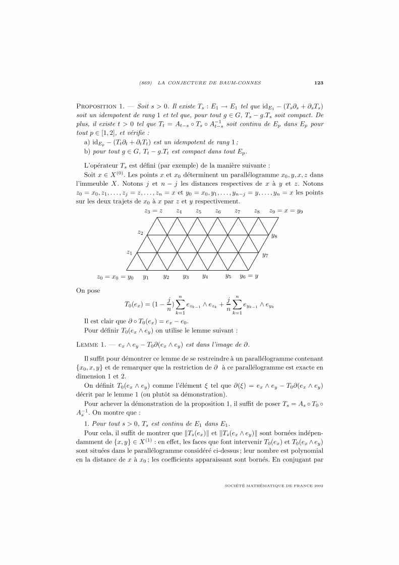
(869) LA CONJECTURE DE BAUM-CONNES 123
Proposition 1. — Soit s > 0. Il existe Ts : E1 → E1 tel que idE1 − (Ts∂s + ∂sTs)soit un idempotent de rang 1 et tel que, pour tout g ∈ G, Ts − g.Ts soit compact. Deplus, il existe t > 0 tel que Tt = At−s Ts A−1
t−s soit continu de Ep dans Ep pourtout p ∈ [1, 2], et verifie :
a) idEp − (Tt∂t + ∂tTt) est un idempotent de rang 1 ;b) pour tout g ∈ G, Tt − g.Tt est compact dans tout Ep.
L’operateur Ts est defini (par exemple) de la maniere suivante :Soit x ∈ X(0). Les points x et x0 determinent un parallelogramme x0, y, x, z dans
l’immeuble X . Notons j et n − j les distances respectives de x a y et z. Notonsz0 = x0, z1, . . . , zj = z, . . . , zn = x et y0 = x0, y1, . . . , yn−j = y, . . . , yn = x les pointssur les deux trajets de x0 a x par z et y respectivement.
On pose
T0(ex) = (1 − j
n)
n∑k=1
ezk−1 ∧ ezk+
j
n
n∑k=1
eyk−1 ∧ eyk
Il est clair que ∂ T0(ex) = ex − e0.Pour definir T0(ex ∧ ey) on utilise le lemme suivant :
Lemme 1. — ex ∧ ey − T0∂(ex ∧ ey) est dans l’image de ∂.
Il suffit pour demontrer ce lemme de se restreindre a un parallelogramme contenantx0, x, y et de remarquer que la restriction de ∂ a ce parallelogramme est exacte endimension 1 et 2.
On definit T0(ex ∧ ey) comme l’element ξ tel que ∂(ξ) = ex ∧ ey − T0∂(ex ∧ ey)decrit par le lemme 1 (ou plutot sa demonstration).
Pour achever la demonstration de la proposition 1, il suffit de poser Ts = As T0 A−1
s . On montre que :
1. Pour tout s > 0, Ts est continu de E1 dans E1.Pour cela, il suffit de montrer que ‖Ts(ex)‖ et ‖Ts(ex ∧ ey)‖ sont bornees indepen-
damment de x, y ∈ X(1) : en effet, les faces que font intervenir T0(ex) et T0(ex∧ ey)sont situees dans le parallelogramme considere ci-dessus ; leur nombre est polynomialen la distance de x a x0 ; les coefficients apparaissant sont bornes. En conjugant par
SOCIETE MATHEMATIQUE DE FRANCE 2002

124 G. SKANDALIS
As, on multiplie ces coefficients par un terme qui decroıt exponentiellement, d’ou leresultat.
2. Pour tout s > 0 et tout g ∈ G, Ts − g.Ts ∈ K(E1).Il suffit pour cela de verifier que, quand x, y tend vers l’infini, ‖(Ts − g.Ts)(ex)‖
et ‖(Ts− g.Ts)(ex ∧ ey)‖ tendent vers 0. Pour cela, remarquons que g.T0 est construitcomme T0 mais avec l’origine x0 remplacee par gx0. Si x est loin de x0, les trajetsde x a x0 et de x a g.x0 utilises dans la construction de T0 coıncident pres de x. Parailleurs, ce sont les points pres de x qui « comptent » a cause de la conjugaison parAs.
3. Il existe t > 0 tel que, pour tout p ∈ [1, 2], Tt soit continu de Ep dans Ep et,pour tout g ∈ G, Tt − g.Tt ∈ K(Ep).
La difficulte ici vient de ce que T ∗t (ex ∧ ey) fait intervenir tous les points z tels que
x, y soit sur le trajet de z a x0. Le coefficient apparaissant decroıt en exp(−tϕ(z)) ;le nombre de tels z croıt exponentiellement. Cependant, en prenant t suffisammentgrand, on peut controler la norme 1 de T ∗
t (ex ∧ ey) et celle de T ∗t (ex ∧ ey ∧ ez). Il en
resulte que T ∗t est continu de E1 dans E1, donc que Tt est continu de E∞ dans E∞.
Comme il est continu de E1 dans E1, il est continu de Ep dans Ep pour tout p (parinterpolation). Un raisonnement analogue montre que Tt − g.Tt ∈ K(Ep) pour toutg ∈ G.
En faisant varier u ∈ [s, t] puis p ∈ [1, 2] on dispose a present d’une homotopieentre (E1, ∂s + Ts) et (E2, ∂t + Tt).
Maintenant, pour achever la demonstration du theoreme, on va utiliser les deuxfaits suivants : pour s tendant vers 0, ∂s devient de plus en plus G-invariant « donc »(E1, ∂s + Ts) tend vers 1 ; pour t tendant vers +∞, (E2, ∂t + Tt) ressemble de plus enplus a γ.
Pour mettre en œuvre cette idee, Lafforgue procede de la maniere suivante :On peut construire une homotopie entre (E1, ∂s + Ts) et (Es
1 , ∂ + T0) ou Es1 est
l’espace de Banach, gradue par 0, 1, 2 dont la composante de degre i est l’espace 1
de X(i) a poids esϕ. Notons que l’action de G dans Es1 n’est plus isometrique ; c’est
pour cela qu’on doit ici quitter KKbanG (C,C) et le remplacer par KKban
G,s(C,C).
ASTERISQUE 276
(869) LA CONJECTURE DE BAUM-CONNES 125
Pour montrer que la classe de (Es1 , ∂ + T0) est 1 et celle de (E2, ∂t + Tt) est γ, on
utilise quelques lemmes generaux de KK-theorie banachique.Soient G un groupe localement compact muni d’une fonction longueur , A, B des
algebres de Banach, E une B paire Z/2Z-graduee munie d’actions de A et de G
« controlees par » (au sens de 3.6). Notons D l’ensemble des morphismes S de E
tels que [S, a] (pour tout a ∈ A) et g.S − S (pour tout g ∈ G) soient dans K(E) etg → g.S soit normiquement continu. Remarquons que tout F ∈ D de degre 1 tel queidE − F 2 ∈ K(E) definit un element de KKban
G, (A, B).
Lemme 2. — Soit S ∈ D de degre 1 tel que S2 ∈ K(E).a) Supposons qu’il existe un morphisme T ∈ D de degre 1 tel que idE − (TS + ST )
soit compact. Alors, il existe un tel T avec en plus T 2 compact. Dans ce cas (E, S+T )est un element de KKban
G, (A, B).b) Dans ce cas, la classe de (E, S + T ) dans KKban
G, (A, B) ne depend pas de T .
En effet, dans a) il suffit de remplacer T par TST , en remarquant que, moduloK(E), ST = (idE − TS), donc TS et ST commutent, donc STTS ∈ K(E) ; on endeduit aussi que ST − STST qui est egal, modulo K(E) a STTS est dans K(E) ; dememe TS − TSTS ∈ K(E).
Pour montrer b), il suffit de remarquer que l’ensemble des T ∈ D tels que ST +TS − idE ∈ K(E) est un sous-espace affine de D.
Lemme 3. — Soient S, S′ ∈ D de degre 1 tels que S2 ∈ K(E) et (S′)2 ∈ K(E).Supposons que le spectre dans l’algebre de Banach quotient D/K(E) de SS′ + S′S nerencontre pas R− . Alors :
a) Il existe T, T ′ ∈ D tels que T 2, (T ′)2, idE−(ST+TS), idE−(S′T ′+T ′S′) ∈ K(E).b) Les classes de (E, S + T ) et (E, S′ + T ′) dans KKban
G, (A, B) coıncident.
Raisonnons dans l’algebre de Banach quotient D/K(E). On a (SS′ + S′S)S =SS′S = S(SS′+S′S) ; de meme, S′(SS′+S′S) = (SS′+S′S)S′. Donc (SS′+S′S)−1
commute avec S et S′. On pose T = S′(SS′+S′S)−1 et T ′ = S(SS′+S′S)−1. De plus,comme le spectre de SS′ + S′S ne rencontre pas R−, on peut definir un logarithmede SS′ + S′S. On obtient une homotopie S(SS′ + S′S)−t + S′(SS′ + S′S)t−1 entreS + T et S′ + T ′.
Lemme 4. — Soient S, T ∈ D de degre 1. On suppose T 2 ∈ K(E), que S commuteexactement a A et a G, que S2 = 0 et , ST +TS = idE. Alors la classe de (E, S +T )dans KKban
G, (A, B) est nulle.
On peut remplacer T par TST . Dans ce cas on a T 2 = 0. Comme S commute avecles elements de A et de G, le sous-espace S(E) de E est invariant par ces elements.Dans la decomposition E = S(E)⊕ T (E), la matrice de ces elements est de la forme(
c1,1 c1,2
0 c2,2
). Notons que c1,2 est dans K(E) car T ∈ D. Il suffit de changer ces actions
SOCIETE MATHEMATIQUE DE FRANCE 2002
126 G. SKANDALIS
en(
c1,1 00 c2,2
)a travers une homotopie
(c1,1 tc1,2
0 c2,2
)(t ∈ [0, 1]). Au bout de cette
homotopie, S + T commute exactement avec A et G et (S + T )2 = idE . Le lemme enresulte facilement.
Pour finir la demonstration du theoreme, notons u la classe dans KKbanG,s(C,C)
de (Es1 , ∂ + T0) ; posons F = Es
1 ⊕C ou C est muni de l’action triviale de G et estde degre 1 pour la graduation. Prolongeons ∂ de F dans F en posant ∂(ex) = 1 ∈ Cpour tout x ∈ X(0) et posons T0(1) = ex0 . Il est facile de voir que la classe de cetelement est u− 1 (ou plutot u — l’image de 1). Par le lemme 4 applique a S = ∂, ontrouve donc que u et l’image de 1 dans KKban
G,s(C,C) coıncident.
Pour montrer que la classe de (E2, ∂t + Tt) est l’image de γ, on commence d’abordpar modifier tres legerement F1 en un operateur F2 : le vecteur λ′ey + µ′ez par lequelon prend le produit exterieur est normalise en norme 1 au lieu de l’etre en norme 2.Il suffit alors, par le lemme 3, de demontrer que le spectre de ∂tF2 + F2∂t est disjointde R−. Pour cela, on remarque que l’image par (∂tF2 + F2∂t)− idE2 d’une face f estportee par des faces voisines, plus proches de x0 que f . Donc, pour t assez grand, lerayon spectral de (∂tF2 + F2∂t)− idE2 est < 1.
4.2. Les autres cas
4.2.a. Le cas « combinatoire »
Dans ce cas, la construction est exactement la meme. La seule chose qui devientreellement plus difficile ici est la demonstration du fait que le complexe ∂ est acyclique.
4.2.b. Le cas « geometrique »
Soient M une variete riemannienne complete, connexe, simplement connexe, decourbure sectionnelle negative ou nulle (bornee inferieurement) et G un groupe loca-lement compact agissant sur M par isometries.
Soit x0 un point de M et notons ϕ : M → R l’application donnee par ϕ(x) =exp(√
d(x, x0)2 + 1).
Dans ce cas, on remplace le bord de la cohomologie simpliciale par la cohomologiede de Rham. On est amene a travailler avec des espaces W (p, k, s− k, ϕt) : espace deSobolev Lp, des k formes s− k fois differentiables a poids ϕt (s est, par exemple, ladimension de l’espace M).
Une difficulte qui apparaıt ici est que le calcul pseudodiffereniel ne marche bien quepour p ∈]0, +∞[. Cependant, t > 0 etant choisi, le complexe de de Rham (W (p, k, s−k, ϕt), d) est acyclique pour p assez proche de +∞.
Le reste de la construction est essentiellement le meme que dans le cas « combina-toire ».
ASTERISQUE 276

(869) LA CONJECTURE DE BAUM-CONNES 127
Je dois cependant dire que, bien que je sois absolument convaincu que la construc-tion marche aussi bien que dans le cas combinatoire, je n’ai pas encore verifie tous lesdetails du cas geometrique.
5. FIN DE LA DEMONSTRATION
Soit G un groupe localement compact operant proprement et isometriquement surune variete riemannienne complete de courbure sectionnelle negative ou nulle ou surun immeuble affine. D’apres ce qui precede, G possede un element γ et γ = 1 dans laKK-theorie banachique. Donc, pour etablir la conjecture de Baum-Connes, il suffitde construire une completion inconditionnelle A de Cc(G) telle que le morphismeA→ C∗
r (G) induise une surjection au niveau des groupes K0.
5.1. Cas des groupes de Lie
Si G est un groupe de Lie semi-simple, reel ou p-adique, Lafforgue ([36]) montreque certaines variantes de l’espace de Schwarz (ou algebre de Harish-Chandra) de G
fournissent des completions inconditionnelles de Cc(G) qui permettent de terminer lademonstration. On obtient ainsi une preuve plus directe de resultats de Wassermanndans le cas reel ([50]) et une generalisation de Baum, Higson et Plymen dans le casp-adique ([6]).
5.2. Propriete (RD) de Haagerup-Jolissaint
Soient G un groupe discret, une fonction longueur sur G (i.e. une applicationG → R+ telle que (e) = 0, (xy) ≤ (x) + (y) pour tout x, y ∈ G). NotonsH∞(G, ) l’espace vectoriel des fonctions f : G → C telles que, pour tout p ∈ R+,∑x∈G
(x)p|f(x)|2 <∞. Si G est finiment engendre, on note H∞(G) l’espace H∞(G, )
ou est la fonction longueur associee a un systeme fini de generateurs (l’espace H∞(G)n’en depend pas).
Dans [16], Haagerup a demontre :
Proposition 1. — Si G est un groupe libre a un nombre fini de generateurs,H∞(G) ⊂ C∗
r (G).
En effet :Pour p ∈ N, notons χp la fonction caracteristique des mots de longueur p (pour un
systeme libre de generateurs). Soient f, g : G→ C des fonctions. On utilise le lemmesuivant :
Lemme 1. — Pour tout p, q, n ∈ N, on a ‖((fχp) (gχq))χn‖2 ≤ ‖fχp‖2‖gχq‖2. Deplus si ((fχp) (gχq))χn = 0, alors n est compris entre |p− q| et p + q et a la memeparite que p + q.
SOCIETE MATHEMATIQUE DE FRANCE 2002

128 G. SKANDALIS
On peut evidemment supposer que f = fχp et g = gχq.La contrainte sur n est claire. Ecrivons p = p1 + r, q = q1 + r et n = p1 + q1.
Notons Ck l’ensemble des mots de longueur k.Soient x, y, z ∈ G de longueur respective p, q, n tels que xy = z. Ecrivons x =
x1x2 ou x1 ∈ Cp1 et x2 ∈ Cr et y = y2y1 ou y1 ∈ Cq1 et y2 ∈ Cr (ces elementssont uniquement determines par x et y). Comme xy est de longueur n on voit quenecessairement z = x1y1 et y2 = x−1
2 . Notons que x1 et y1 sont entierement determinespar z.
Il s’ensuit que
|f g(z)| =∣∣∣ ∑u∈Cr
f(x1u)g(u−1y1)∣∣∣ ≤ (∑
u∈Cr
|f(x1u)|2)1/2(∑
u∈Cr
|g(uy1)|2)1/2
par l’inegalite de Cauchy-Schwarz.On a alors
‖(f g)χn‖22 =∑
x1∈Cp1 , y1∈Cq1 , x1y1∈Cn
|f g(x1y1)|2
≤∑
x1∈Cp1 , y1∈Cq1 , x1y1∈Cn
(∑u∈Cr
|f(x1u)|2)(∑
u∈Cr
|g(uy1)|2)
≤∑
x1∈Cp1 , y1∈Cq1
(∑u∈Cr
|f(x1u)|2)(∑
u∈Cr
|g(uy1)|2)
= ‖f‖22‖g‖22 .
La proposition 1 se deduit tres facilement du lemme 1 :On ecrit 2(G) comme somme hilbertienne de 2(Cr).Soient f ∈ Cc(G) et p ∈ N. L’operateur de convolution a gauche par (fχp) peut etre
vu dans la decomposition ci-dessus comme une matrice Tr,s ou Tr,s : 2(Cs)→ 2(Cr)est un operateur de norme ≤ ‖(fχp)‖2, nul si |r − s| ≥ p, ou si r − s n’est pas dela meme parite que p. On peut ecrire T comme somme des p + 1 operateurs Sk ouSk est l’operateur de matrice Tr,s avec r − s = −p + 2k (0 ≤ k ≤ p). Il est clair que‖λ(fχp)‖ ≤
∑k ‖Sk‖ ≤ (p + 1)‖(fχp)‖2. Il vient
‖λ(f)‖ ≤∑
(p + 1)‖fχp‖2 ≤ (∑
(p + 1)−2)1/2∑
p
((p + 1)4‖fχp‖22)1/2
par l’inegalite de Cauchy-Schwartz, d’ou la proposition.On peut en fait, a partir du lemme 1, demontrer :
Proposition 2. — Si G est un groupe libre a un nombre fini de generateurs, H∞(G)est une sous-algebre de C∗
r (G) stable par calcul fonctionnel holomorphe. En particulier,l’inclusion H∞(G) → C∗
r (G) induit un isomorphisme au niveau de la K-theorie.
Cette idee est reprise par Jolissaint ([22]). Il donne la definition suivante :
ASTERISQUE 276

(869) LA CONJECTURE DE BAUM-CONNES 129
Definition 2. — On dit qu’un groupe finiment engendre G possede la propriete(RD) si H∞(G) ⊂ C∗
r (G).
Il demontre que si G a la propriete (RD), alors H∞(G) est une sous-algebre deC∗
r (G) stable par calcul fonctionnel. En fait (cf. [23]), il existe r ∈ N tel que l’ensembleAr = f ∈ CG,
∑x∈G
(x)r|f(x)|2 < ∞ est une sous-algebre de C∗r (G) stable par calcul
fonctionnel holomorphe.
Remarquons que Ar est une algebre de Banach et une completion inconditionnelle.
5.3. Groupes possedant la propriete (RD)
Jolissaint ([22]) etend le travail de Haagerup en demontrant que plusieurs groupesse comportant comme les groupes libres, en particulier les sous-groupes cocompactsdes groupes de Lie reels simples de rang 1, ont la propriete (RD).
Ce resultat est lui-meme etendu par de la Harpe ([17]) aux groupes hyperboliquesde Gromov.
Tres recemment, Ramagge, Robertson et Steger ([41]) ont etabli la propriete (RD)pour des groupes discrets operant proprement avec quotient compact sur un immeubleA2. Leur resultat contient en particulier les reseaux cocompacts de SL3(F) ou F estun corps local non archimedien.
Comme dans la demonstration de Haagerup, on doit analyser les couples x, y ayantun produit donne. On est amene a etudier les triangles dans l’immeuble. La cle de lademonstration est que tout triangle se contracte uniquement sur un triangle equilateraldans un appartement.
Lafforgue enfin, en remplacant certaines egalites par des estimations, a adapte lademonstration de Ramagge, Robertson et Steger au cas des sous-groupes cocompactsde SL3(R) et SL3(C) (cf. [34]).
5.4. Limite de la methode
D’apres une conjecture de Valette ([49]), tout sous-groupe cocompact d’un groupede Lie simple devrait posseder la propriete (RD).
Cependant, la methode a ses limites : plusieurs sous-groupes discrets (non cocom-pacts) de groupes de Lie ne possedent pas la propriete (RD) du fait de l’existenced’elements paraboliques. Par exemple, les seuls groupes moyennables possedant lapropriete (RD) sont les groupes a croissance polynomiale (cf. [22]). De plus cettemethode marche tres mal pour les produits croises — et ne permet de demontrer laconjecture de Baum-Connes a coefficients que dans des cas tres particuliers (cf. [37]).
SOCIETE MATHEMATIQUE DE FRANCE 2002

130 G. SKANDALIS
6. QUELQUES AUTRES AVANCEES RECENTES
En plus du resultat de Lafforgue que nous venons de discuter, il y a eu recemmentquelques autres avancees significatives sur la conjecture de Baum-Connes et des sujetsconnexes.
6.1. Actions moyennables ([18])
N. Higson vient de faire une remarque tres simple et astucieuse qui permet d’etablirl’injectivite de l’homomorphisme de Baum-Connes (a coefficients) pour les groupesdiscrets possedant une action moyennable sur un espace compact.
La moyennabilite d’un groupe est une notion degagee depuis plusieurs decennies.On dispose a present de plusieurs proprietes equivalentes. De plus, cette notion a eteetendue aux actions de groupes et aux groupoıdes. Nous renvoyons a l’excellente mo-nographie [2] pour une discussion tres actuelle sur toutes les notions de moyennabilite.
Du point de vue des C∗-algebres, un groupe localement compact G est moyennablesi C∗(G) = C∗
r (G). Une action de G sur un espace compact X est moyennable siC(X) G = C(X) r G.
Rappelons que Higson et Kasparov ont demontre la conjecture de Baum-Connespour tout groupe moyennable, et que Tu a etendu ce resultat au cas des groupoıdesmoyennables.
Toute action d’un groupe moyennable est moyennable. Cependant, plusieursgroupes, bien que non moyennables, possedent des actions moyennables sur desespaces compacts. Par exemple, G = SLn(R) n’est pas moyennable pour n ≥ 2, maisson action dans l’espace compact des drapeaux G/P est moyennable ou P designe lesous-groupe de SLn(R) forme des matrices triangulaires superieures (a coefficientsdiagonaux positifs).
La demonstration de Higson est (un peu schematiquement) la suivante :Si l’action de G dans un espace compact X est moyennable, son action dans l’espace
M des mesures de probabilite sur X , muni de la topologie de la convergence vagueest moyennable.
Soit A une C∗-algebre munie d’une action de G. Notons B la C∗-algebre C(M ; A)des fonctions continues de M dans A. L’homomorphisme A→ B qui a a ∈ A associela fonction constante egale a a etant equivariant, on obtient un homomorphisme Ar
G → B r G, d’ou un homomorphisme de groupes de K-theorie. De meme, on a unhomomorphisme K0,top(G; A) → K0,top(G; B). On obtient un diagramme commutatif
K0,top(G; A)µA
G−→ A r G
↓ ↓
K0,top(G; B)µB
G−→ B r G
ASTERISQUE 276

(869) LA CONJECTURE DE BAUM-CONNES 131
Or, l’action de G dans M etant moyennable, par la generalisation par Tu ([48]) dutheoreme de Higson-Kasparov, l’homomorphisme de Baum-Connes µB
G est un isomor-phisme. De plus, comme M est contractile, l’application A → B est une equivalenced’homotopie, d’ou l’on deduit que l’homomorphisme K0,top(G; A) → K0,top(G; B) estaussi un isomorphisme. En fait pour avoir l’isomorphisme ici, Higson doit supposerque le groupe G est discret, il utilise un modele simplicial pour EG et une suite exactede Mayer-Vietoris. Il s’ensuit que l’homomorphisme µA
G est injectif (et scinde).
On peut facilement obtenir un resultat legerement plus fort que celui de Higsonen remplacant la condition de moyennabilite de l’action de G par l’existence d’unplongement uniforme de G dans un espace hilbertien (au sens ci-dessous, cf. [46]).
6.2. Conjecture de Baum-Connes et geometrie « a l’infini » ([43], [51])
Le resultat de [18] cite ci-dessus (ainsi que sa generalisation [46]) avait d’abordete demontre par Yu dans [51] sous l’hypothese que G etait sans torsion et BG uncomplexe cellulaire fini(6).
Le demonstration de Yu est tout a fait differente de celle de Higson : elle utilise lelangage de la geometrie « grossiere » (coarse), je dirais plutot geometrie a l’infini.
Il s’agit la de tout un monde — et il n’est pas possible de citer ici toutes les contri-butions importantes dans le sujet. Nous renvoyons a [43] et [51] pour une discussiondetaillee de toutes ces notions.
Il est apparu (cf. [14]) que la conjecture de Novikov pour un groupe discret G esten fait assez peu dependante de la structure de groupe. La seule chose qui compte estla structure a l’infini de G.
Soit (X, d) un espace metrique. De meme que pour une structure uniforme, unestructure a l’infini de X est basee sur les ensembles de la forme ∆r = (x, y) ∈X ×X, d(x, y) < r (pour r ∈ R+). Cependant on s’interesse a r grand.
On dit qu’une partie U ⊂ X ×X est un entourage pour la structure a l’infini s’ilest contenu dans un ensemble ∆r.
Le role des applications uniformement continues est joue ici par les applicationsf : X → Y telles que l’image directe de tout entourage soit un entourage (autrementdit ∀r ∈ R+, ∃R ∈ R+, d(x, x′) ≤ r ⇒ d(f(x), f(x′)) ≤ R).
Une application f : X → Y est un plongement uniforme si, pour toute partie U deX ×X , U est un entourage si et seulement si f(U) est un entourage.
A un espace metrique, on associe une C∗-algebre construite de la maniere suivante :on fixe un espace hilbertien H et une representation π : C0(X) → L(H) telle queπ−1(K(H)) = 0 et π(C0(X))H = H . Le support d’un element T ∈ L(H) est le pluspetit ferme F de X × X tel que si f, g ∈ C0(X) sont telles que (x, y) → f(x)g(y)est nulle sur F , alors π(f)Tπ(g). La C∗-algebre de X est l’adherence de l’ensemble
(6)C’est Higson et Roe dans [21] qui ont reformule le theoreme de [51] en termes de moyennabilite.
SOCIETE MATHEMATIQUE DE FRANCE 2002

132 G. SKANDALIS
des operateurs T ∈ L(H) dont le support est un entourage et tels que, pour toutf ∈ C0(X), Tπ(f) et π(f)T sont compacts.
Il y a aussi une conjecture de Baum-Connes qui predit la K-theorie de cetteC∗-algebre (cf. [43]), du moins si X est a geometrie a l’infini bornee. Rappelonsqu’un espace metrique X est dit a geometrie a l’infini bornee si, pour tout r ∈ R+,il existe N ∈ N tel que le nombre d’elements de toute partie de X de diametre ≤ r
est borne par N .Le lien avec la conjecture de Baum-Connes est le suivant : soit G un groupe finiment
engendre. Munissons-le de la distance invariante a gauche associee a la longueur demots (par rapport a un systeme fini de generateurs). Si G n’a pas de torsion et BG
est un complexe cellulaire fini, la conjecture de Baum-Connes a l’infini pour l’espacemetrique G implique l’injectivite de µG,r.
En utilisant une variante de la methode de Higson-Kasparov, Yu ([51], voir aussi[46] pour une autre demonstration de ce resultat) montre :
Theoreme 1. — Tout espace metrique a geometrie a l’infini bornee qui admet unplongement uniforme dans un espace hilbertien satisfait la « conjecture de Baum-Connes a l’infini ».
REFERENCES
[1] C. Anantharaman-Delaroche – Classification des C∗-algebres purement in-finies nucleaires (d’apres E. Kirchberg), Sem. Bourbaki 1995/96, exp. no 805,Asterisque 241 (1997), 7-27.
[2] C. Anantharaman-Delaroche et J. Renault Amenable groupoids (preprint1999), a paraıtre a Ens. Math.
[3] M.F. Atiyah – Elliptic operators discrete groups and von Neumann algebras,Asterisque 32-33 (1976), 43-72.
[4] P. Baum and A. Connes – K-theory for Lie groups and foliations (preprint1982), a paraıtre a Ens. Math.
[5] P. Baum, A. Connes and N. Higson – Classifying space for proper actions andK-theory of group C∗-algebras, Contemporary Math. 167 (1994), 241-291.
[6] P. Baum, N. Higson and R. P Lymen – A proof of the Baum-Connes conjecturefor p-adic GL(n), C. R. Acad. Sci. Paris, Ser. I Math. 325, no 2 (1997), 171-176.
[7] J.-B. Bost – Principe d’Oka, K-theorie et systemes dynamiques non commuta-tifs, Inv. Math. 101 (1990), 261-333.
[8] J. Chabert – Stabilite de la conjecture de Baum-Connes pour certains produitssemi-directs de groupes, C. R. Acad. Sci. Paris, Ser. I Math. 328, no 12 (1999),1129–1132.
ASTERISQUE 276

(869) LA CONJECTURE DE BAUM-CONNES 133
[9] A. Connes – Sur la theorie non commutative de l’integration, Lect. Notes inMath. 725 (1979), 19-143.
[10] J. Cuntz – K-theoretic amenability for discrete groups, J. Reine ang. Math. 344(1983), 180-195.
[11] J. Cuntz – Bivariante K-theorie fur lokalconvexe Algebren und der Chern-Connes Character, Doc. Math. 2 (1997), 139-182.
[12] C. Delaroche et A.A. Kirillov – Sur les relations entre l’espace dual d’ungroupe et la structure de ses sous-groupes fermes (d’apres D. A. Kazhdan), Sem.Bourbaki 1967/68, exp. n 343, Soc. Math. France 10 (1995), 507-528.
[13] T. Fack – K-theorie bivariante de Kasparov, Sem. Bourbaki 1982/83, Asterisque105-106, (1983), 149-166.
[14] M. Gromov – Geometric reflections on the Novikov conjecture, Novikov conjec-tures, index theorems and rigidity, Vol. 1 (Oberwolfach, 1993), London Math.Soc. Lecture Note Ser. 226 Cambridge Univ. Press (1995), 164–173.
[15] M. Gromov – Spaces and questions (1999).[16] U. Haagerup – An example of a nonnuclear C∗-algebra which has the metric
approximation property, Inv. Math. 50 (1979), 279-293.[17] P. de la Harpe – Groupes hyperboliques, algebres d’operateurs et un theoreme
de Jolissaint, C. R. Acad. Sci. Paris, Ser. I Math. 307 (1988), 771-774.[18] N. Higson – Bivariant K-theory and the Novikov conjecture (1999).[19] N. Higson and G. Kasparov – Operator K-theory for groups which act properly
and isometrically on Hilbert space, Electronic Research Anouncements, AMS 3(1997), 131-141.
[20] N. Higson, V. Lafforgue and G. Skandalis – Counterexamples to the Baum-Connes Conjectures, en preparation.
[21] N. Higson and J. Roe – Amenable group actions and the Novikov conjecture(1999).
[22] P. Jolissaint – Rapidly decreasing functions in reduced C∗-algebras of groups,Trans. Amer. Math. Soc. 317 (1990), 167-196.
[23] P. Jolissaint – K-theory of reduced C∗-algebras and rapidly decreasing functionson groups, K- theory 2 (1989), 723-735.
[24] P. Julg – Remarks on the Baum-Connes conjecture and Kaszdan’s property T ,Fields Inst. Comm. 13 (1997), 145-153.
[25] P. Julg – Travaux de N. Higson et G. Kasparov sur la conjecture de Baum-Connes, Sem. Bourbaki, vol. 1997/98, exp. n 841, Asterisque 252 (1998), 151-183.
[26] P. Julg et A. Valette – Fredholm modules associated to Bruhat-Tits Buildings,Proc. of the Center for Math. Analysis, Australian National University 16 (1988),143-155.
SOCIETE MATHEMATIQUE DE FRANCE 2002

134 G. SKANDALIS
[27] G.G. Kasparov – Hilbert C∗-modules : theorems of Stinespring and Voiculescu,J. Operator Theory 4 (1980), 133-150.
[28] G.G. Kasparov – The operator K-functor and extensions of C∗-algebras, Math.USSR Izv. 16 (1981), n 3, 513-572. Translated from : Izv. Akad. Nauk. S.S.S.R.Ser. Mat. 44 (1980), 571-636.
[29] G.G. Kasparov – Equivariant KK-theory and the Novikov conjecture, Inv.Math. 91 (1988), 147-201.
[30] G.G. Kasparov and G. Skandalis – Groups acting on buidings, OperatorK-theory and Novikov’s conjecture, K-theory 4 (1991), 303-337.
[31] G.G. Kasparov and G. Skandalis – Groupes « boliques » et conjecture de No-vikov, Note C.R.A.S. 319, Ser. I (1994), 815-820.
[32] D. Kazhdan – Connection of the dual space of a group with the structure of itsclosed subgroups, Funct. Anal. and its Appl. 1 (1967), 63-65.
[33] V. Lafforgue – Une demonstration de la conjecture de Baum-Connes pour lesgroupes reductifs sur un corps p-adique et pour certains groupes discrets possedantla propriete (T), C. R. Acad. Sci. Paris, Ser. I Math. 327, no 5 (1998), 439-444.
[34] V. Lafforgue – A proof of property (RD) for discrete cocompact subgroups ofSL3(R) (preprint 1998), a paraıtre a Journal of Lie theory.
[35] V. Lafforgue – K-theorie bivariante pour les algebres de Banach et conjecturede Baum-Connes (preprint 1998).
[36] V. Lafforgue – Espaces de Schwartz (preprint 1998).
[37] V. Lafforgue – K-theorie bivariante pour les algebres de Banach, groupoıdeset conjecture de Baum-Connes (preprint en preparation 1999).
[38] P.-Y. Le Gall – Theorie de Kasparov equivariante et groupoıdes, C. R. Acad.Sci. Paris, Ser. I Math. 324, n 6 (1997), 695-698.
[39] A.S. Miscenko – Homotopy invariance of non simply connected manifolds, I :Rational invariance, Math. USSR Izv. 4 (1970), 509-519, transl from Izv. Akad.Nauk. SSSR Ser. Math. 34, (1970), 501-514.
[40] H. Oyono-Oyono – La conjecture de Baum-Connes pour les groupes agissantsur les arbres, C. R. Acad. Sci. Paris, Ser. I Math. 326, no 7 (1998), 799-904.
[41] J. Ramagge, G. Robertson and T. Steger – A Haagerup inequality for A1×A1 and A2 buildings, Geometric and Funct. Anal. 8, n 4 (1998), 702-731.
[42] J.N. Renault – A groupoid approach to C∗-algebras, Lecture Notes in Math.793, Springer-Verlag, New York (1980).
[43] J. Roe – Index Theory, Coarse Geometry, and Topology of Manifolds, CBMSRegional Conf. Series in Math. 90, AMS (1996).
[44] G. Skandalis – Une notion de nuclearite en K-theorie (d’apres J.Cuntz),K-theory 1 (1988), 549-573.
ASTERISQUE 276

(869) LA CONJECTURE DE BAUM-CONNES 135
[45] G. Skandalis – Approche de la conjecture de Novikov par la cohomologie cy-clique. D’apres Connes-Gromov-Moscovici, Sem. Bourbaki, vol. 1990/91, exposeno 739, Asterisque 201-202-203 (1992), 299-316.
[46] G. Skandalis, J.L. Tu and G. Yu – Coarse Baum-Connes conjecture and Grou-poids (preprint 1999).
[47] J.L. Tu – La conjecture de Novikov pour les feuilletages hyperboliques, K-theory16, n 2 (1999), 129-184.
[48] J.L. Tu – La conjecture de Novikov pour les feuilletages moyennables, K-theory17, n 3 (1999), 215-264.
[49] A. Valette – Questions, Novikov conjectures, index theorems and rigidity, Vol. 1(Oberwolfach, 1993), London Math. Soc. Lecture Note Ser. 226, Cambridge Univ.Press (1995), p. 74.
[50] A. Wassermann – Une demonstration de la conjecture de Connes-Kasparov pourles groupes de Lie lineaires connexes reductifs, C. R. Acad. Sci. Paris, Ser. I Math.304 (1987), 559-562.
[51] G. Yu – The coarse Baum-Connes conjecture for spaces which admit uniformembeddings into Hilbert space (preprint 1999), a paraıtre a Inv. Math.
Georges SKANDALIS
UMR 7586 du C.N.R.S.Universite de Paris VIICase Postale 70122, place JussieuF-75251 PARIS Cedex 05E-mail : [email protected]
SOCIETE MATHEMATIQUE DE FRANCE 2002

Seminaire BOURBAKI Mars 200052e annee, 1999-2000, no 870, p. 137 a 159
THEORIE DES MODELESET CONJECTURE DE MANIN-MUMFORD
[d’apres Ehud Hrushovski]
par Elisabeth BOUSCAREN
1. INTRODUCTION
Je vais presenter ici l’une des applications recentes de la theorie des modeles a lageometrie diophantienne, la nouvelle demonstration, due a E. Hrushovski ([Hr2]), de laconjecture de Manin-Mumford (generalisee) qui est basee sur l’etude, du point de vuede la theorie des modeles, des corps algebriquement clos munis d’un automorphisme.
Theoreme 1.1 (Conjecture de Manin-Mumford). — Soit G un groupe algebriquecommutatif connexe defini sur un corps de nombres k et X une sous-variete de G.Alors il y a un nombre fini de points de torsion de G, a1, . . . , aM , et de sous-groupesalgebriques de G, G1, . . . , GM tels que pour chaque i, ai + Gi est contenu dans X et
X(kalg) ∩ Tor(G) =M⋃i=1
ai + Tor(Gi).
De plus on peut borner de facon effective le nombre M de translates : il existe c, e
deux constantes ne dependant que d’invariants lies a G (et non a X) et du choix dedeux premiers de bonne reduction pour G, tels que M ≤ c deg(X)e.
En utilisant des methodes de calcul assez grossieres, on obtient que les constantesc et e sont doublement exponentielles.
La demonstration de Hrushovski passe par une premiere etape ou il prend unpremier de bonne reduction pour G, de caracteristique residuelle p, et montre leresultat pour la torsion premiere a p, c’est-a-dire pour le sous-groupe Torp′(G) deselements de torsion de G dont l’ordre n’est pas divisible par p. On obtient dans ce casque
X(kalg) ∩ Torp′(G) =N⋃
i=1
ai + Torp′(Gi),
SOCIETE MATHEMATIQUE DE FRANCE 2002

138 E. BOUSCAREN
ou il est facile de montrer directement que N ≤ a deg(X)b, avec a doublementexponentiel (en la dimension de A, le degre de l’addition dans A et la cardinalite ducorps residuel) et b exponentiel en la dimension de A.
Le but de cet expose, en presentant la demonstration de Hrushovski, est d’essayerd’expliquer pourquoi la theorie des modeles a quelque chose a dire sur ce type dequestions et aussi de donner une idee des resultats qu’on montre et des outils qu’ondeveloppe en theorie des modeles.
Nous passerons donc rapidement sur les parties purement « geometrie algebrique »de la demonstration.
De meme, la tres breve presentation historique et bibliographique qui suit n’a, celasera visible tout de suite, aucune pretention d’exhaustivite.
1.1. Petit historique et conjecture de Lang
La conjecture de Manin-Mumford originelle porte sur l’intersection d’une courbeavec les points de torsion d’une variete abelienne. Elle a ete tout d’abord demontreepar M. Raynaud ([Ra1]), puis R. Coleman ([Col]) en a donne une autre demonstrationpar des methodes tres differentes ; Raynaud a ensuite ([Ra2]) demontre le resultatpour une sous-variete quelconque, puis M. Hindry ([Hi1]), en s’inspirant d’une ideede S. Lang ([La1]) pour le cas des courbes, a demontre le resultat general pour ungroupe algebrique commutatif.
On trouve une autre approche de ces questions dans les travaux sur la conjecturede Bogomolov, on se contentera ici de renvoyer a l’expose de A. Abbes sur le sujetdans le cadre de ce seminaire ([Ab]) et aux travaux recents de S. David et P. Philippon([DaPh]).
En revanche, nous allons dire quelques mots de la conjecture de Lang (dite aussiconjecture de Mordell-Lang), enoncee par Lang dans [La1] et qui regroupe dans uncadre general la conjecture de Manin-Mumford et la conjecture de Mordell (voir aussipar exemple [La2]).
Nous l’enoncons ici pour la caracteristique zero :
Conjecture de Lang (absolue). — Soient K un corps algebriquement clos de ca-racteristique zero, A une variete abelienne definie sur K, X une sous-variete de A
definie sur K et Γ un sous-groupe de A(K) de rang fini. Alors il existe γ1, . . . , γn ∈ Γet B1, . . . , Bn sous-varietes abeliennes de A tels que γi + Bi ⊂ X et
X(K) ∩ Γ = ∪ni=1γi + (Bi(K) ∩ Γ).
Cette conjecture a finalement ete demontree par G. Faltings ([Fa]) apres de nom-breux travaux entre autres de Manin, Vojta, Laurent, Hindry et Faltings lui-meme.On peut trouver des bibliographies recentes, commentees et completes, dans [Hi2]ou [Maz]. L’extension au cas des varietes semi-abeliennes est due a Vojta([Voj]) etMcQuillan ([McQ]).
ASTERISQUE 276

(870) THEORIE DES MODELES ET CONJECTURE DE MANIN-MUMFORD 139
Si on veut etendre cette conjecture au cas de caracteristique non nulle, il fautse contenter d’une version relative, dite aussi conjecture de Lang pour les corps defonctions. En voici un enonce un peu simplifie :
Conjecture de Lang pour les corps de fonctions. — Soient K0 < K deuxcorps algebriquement clos, A une variete abelienne definie sur K de K/K0-trace zero,et X une sous-variete de A definie sur K. Soit Γ un sous-groupe de rang fini deA(K). Alors il existe γ1, . . . , γn ∈ Γ et B1, . . . , Bn sous-varietes abeliennes de A telsque γi + Bi ⊆ X et
X(K) ∩ Γ = ∪ni=1γi + (Bi(K) ∩ Γ).
On rappelle que Γ est de rang fini si il existe un groupe Γ0 finiment engendretel que, pour chaque γ ∈ Γ, il y a un entier n ≥ 1 tel que nγ ∈ Γ0. Si on est encaracteristique p > 0, on demande que l’entier n ne soit pas divisible par p. Direque A est de K/K0-trace zero est equivalent a dire que A n’a aucune sous-varieteabelienne homomorphe a une variete abelienne definie sur K0.
Dans [Hr1], Hrushovski a donne une demonstration modele-theorique de la conjec-ture de Lang pour les corps de fonctions en toute caracteristique (on peut trouverune presentation de ces resultats dans l’expose [Go] de ce seminaire, ou dans [Pi3],et une exposition plus detaillee dans le livre [Bo]). Pour la caracteristique p > 0, ils’agissait de la premiere demonstration du cas general, les resultats precedents (voir[AbrVo]) necessitant des hypotheses supplementaires. Un peu auparavant, A. Buium([Bu]) avait donne une nouvelle demonstration du cas de caracteristique zero, dontl’idee de depart etait de passer a un corps differentiellement clos et de remplacer legroupe Γ par un groupe ∆-ferme (ou differentiellement algebrique) de dimension finie.C’est cette idee qui est l’inspiration des demonstrations de Hrushovski, pour les deuxresultats, Lang pour les corps de fonctions et Manin-Mumford.
1.2. Le rapport avec la theorie des modeles
L’idee qui est a la base de ces deux demonstrations est donc la suivante : on veutremplacer le sous-groupe Γ (Tor(G) dans notre cas) par un sous-groupe « ferme » ou« algebrique », pour lequel on montrera le resultat. On ne peut pas le faire sans, d’unemaniere ou d’une autre, rajouter des « fermes » supplementaires (c’est-a-dire de lastructure supplementaire), puisque, quand G par exemple est une variete abelienne,la torsion est dense dans G. C’est exactement ce que fait Buium dans [Bu], quandil passe dans un corps differentiellement clos, remplace le groupe Γ par un groupe∆-ferme de dimension finie et utilise ensuite l’arsenal des outils developpes dans cecadre. Or c’est la une methode qui rentre tout a fait dans la problematique develop-pee en theorie des modeles et pour laquelle nous disposons d’un cadre systematique,d’outils et de resultats deja existants. En effet, puisant son inspiration dans la geome-trie algebrique et les geometries combinatoires, la theorie des modeles developpe dansun cadre abstrait des notions d’independance, de dimension et de geometrie. Cela a
SOCIETE MATHEMATIQUE DE FRANCE 2002

140 E. BOUSCAREN
permis d’isoler une notion qui va se retrouver au centre de toutes ces applicationsrecentes : la notion de modularite qui caracterise, a partir du comportement de larelation d’independance, les groupes dans lesquels les seuls sous-ensembles qu’on peutdefinir sont les (combinaisons booleennes finies de) translates de sous-groupes. Mon-trer que le groupe Tor(G) satisfait l’enonce de Manin-Mumford, c’est exactement,une fois qu’on s’est place dans le bon cadre, montrer que c’est un groupe modulaire,nous le verrons dans les sections 2.2 et 2.3 ; et l’on a des outils pour cela.
1.3. Le cadre dans lequel on travaille
On a donc un groupe algebrique, G, defini sur un corps de nombres k. On vaconsiderer un automorphisme σ dans Gal(kalg/k), judicieusement choisi, de manierea ce que la torsion soit contenue dans le sous-groupe Sσ des solutions, dans G(kalg),d’une equation faisant intervenir σ (ce qu’on appelle traditionnellement une equationde difference) qu’on peut explicitement calculer. On plonge alors (kalg, σ) dans ungros corps K sur lequel σ se prolonge et qui est clos en ce sens qu’il contient dejades solutions pour toute equation de difference qui a une solution dans une extension.C’est ce qu’on appellera un corps de difference generique. Et, de meme qu’on a latopologie de Zariski sur un corps algebriquement clos ou la ∆-topologie sur un corpsdifferentiellement clos, on definit une σ-topologie sur K. La theorie des modeles permetd’analyser la structure de K avec ces nouveaux ensembles geometriques. Cette analysea ete faite par Z. Chatzidakis et E. Hrushovski dans [ChHr] qui montrent qu’onpeut y definir une bonne notion d’independance et de dimension. En particulier, ilsdemontrent en caracteristique zero un theoreme de dichotomie, qui dit a peu presque les seuls ensembles de dimension finie qui ne sont pas « modulaires » se trouventdans le corps fixe par σ. A partir de cette analyse et de ce theoreme de dichotomie,Hrushovski trouve un critere « effectif » pour distinguer, parmi les sous-groupes deG(K) definis par des equations de difference, ceux qui sont modulaires. Il ne resteplus qu’a verifier que le sous-groupe Sσ judicieusement choisi plus haut est du bontype, puis a borner le nombre de translates qui vont intervenir par des calculs simplesa partir de l’equation qui definit Sσ.
C’est exactement comme cela que cela se passe dans le cas de la torsion premiere ap. Pour la torsion totale, c’est un peu plus complique, car, s’il est facile, en travaillanta partir de deux premiers de bonne reduction distincts, de montrer qu’il existe uneσ-equation qui s’annule sur la torsion toute entiere et est du bon type, on ne saitpas le faire de maniere effective. Donc, si on veut garder des bornes sur le nombre detranslates, il faut travailler un peu plus, en gardant deux equations distinctes, l’unepour la torsion premiere a p, l’autre pour la p-torsion puis combiner les deux.
Dans une premiere partie, nous allons presenter le cadre modele theorique, c’est-a-dire les corps de difference generiques et les groupes que l’on peut y definir avecdes equations de difference (section 2). Ensuite nous expliquerons comment utiliserles resultats ainsi obtenus pour demontrer la conjecture de Manin-Mumford (section
ASTERISQUE 276

(870) THEORIE DES MODELES ET CONJECTURE DE MANIN-MUMFORD 141
3). En fait, nous traiterons le cas de la torsion premiere a p et ne dirons que quelquesmots sur le passage a la torsion totale. Enfin nous terminerons en mentionnant d’autresapplications de la meme methode (section 4).
Merci a celles et ceux qui ont bien voulu relire tout ou partie de ce texte, ou re-pondre aux nombreuses questions auxquelles je ne pouvais manquer d’etre confrontee,puisqu’il me faut parler ici non seulement de theorie des modeles mais aussi de geome-trie algebrique, domaine qui n’est pas le mien. En particulier, merci a Z. Chatzidakis,F. Delon, D. Bertrand, M. Hindry et aussi a E. Hrushovski. Je suis evidemment seuleresponsable des erreurs qui se seraient ici glissees dans un enonce de theoreme ou dansune esquisse de preuve, a la suite d’une tentative indue de simplification.
2. LES CORPS DE DIFFERENCE GENERIQUES
2.1. Definition et existence
Nous appellerons corps de difference un corps K muni d’un automorphisme distin-gue σ. On peut par exemple considerer K = kalg, la cloture algebrique d’un corps k,muni d’un automorphisme σ ∈ Gal(kalg/k) ou encore, si K est un corps parfait decaracteristique p > 0 et n ≥ 1, K muni de l’automorphisme de Frobenius x → xpn
.Les corps de difference ont ete a l’origine etudies par Ritt dans les annees 30 ; on
peut trouver tous les resultats algebriques de base dans le livre de R. Cohn [Coh](dans ce livre, un corps de difference est un corps avec un monomorphisme distingue ;quand il s’agit d’un automorphisme, le corps est appele corps de difference inversif).
Il etait naturel pour des theoriciens des modeles de s’interesser a la classe des corpsde difference existentiellement clos c’est-a-dire tels que tout systeme fini d’equationsde difference ayant une solution dans une extension du corps en a deja une dans lecorps. C’est l’analogue, pour les corps de difference, des corps algebriquement clos pourles corps, des corps differentiellement clos pour les corps differentiels, ou bien encoredes corps reels clos pour les corps ordonnes. Les premieres proprietes (axiomatisation,decidabilite etc) ont ete etudiees par A. Macintyre, L. van den Dries et C. Wood (voir[Ma1]). Ensuite, une etude plus complete de la structure de ces corps du point devue de la theorie des modeles a ete faite par Z. Chatzidakis et E. Hrushovski dansun premier temps ([ChHr]), puis par les memes avec un troisieme auteur, K. Peterzil([ChHrPe]). C’est dans le premier de ces deux articles que se trouvent les resultatsqui sont utilises pour la demonstration de Manin-Mumford, notamment le resultatde dichotomie en caracteristique zero qui est crucial. Enfin, dans l’article ou il donnesa demonstration de la conjecture de Manin-Mumford ([Hr2]), Hrushovski commencepar pousser plus loin l’etude des groupes commutatifs definissables dans ces corps dedifference. Des la prochaine section, pour simplifier les enonces, nous nous limiteronsa la caracteristique zero et aux resultats ayant un rapport direct avec les applications
SOCIETE MATHEMATIQUE DE FRANCE 2002

142 E. BOUSCAREN
dont nous voulons parler. Pour en savoir plus sans se plonger dans les articles eux-memes, on pourra consulter [Ch2].
Commencons par decrire ces corps, que nous appellerons ici pour simplifier corps dedifference generiques (au depart, dans [ChHr], ils apparaissent comme modeles d’unetheorie appelee ACFA, « algebraically closed fields with an automorphism » ; on lesappelle aussi souvent corps algebriquement clos avec un automorphisme generique).
Convention et notation. — Nous utiliserons le terme de variete uniquement dans lecas irreductible. Si X est une variete affine definie sur K, Xσ est la variete affinedefinie en appliquant σ aux coefficients des equations qui definissent X .
Definition 2.1. — Soit (K, σ) un corps de difference. On dit que (K, σ) est un corpsde difference generique si K est un corps algebriquement clos verifiant la propriete :
(*) Soient X une variete affine definie sur K et Y une sous-variete de X × Xσ
definie sur K, dont les projections sur les facteurs X et Xσ sont denses. Alors ilexiste a ∈ X(K) tel que (a, σ(a)) ∈ Y (K).
Les corps algebriquement clos satisfaisant (*) sont bien exactement les corps dedifference existentiellement clos et tout corps de difference se plonge dans un corps dedifference generique.
Ces corps, comme on va le voir dans la suite, sont munis d’une structure plus richeque celle induite uniquement par la topologie de Zariski mais que l’on sait quandmeme analyser !
Commencons par quelques proprietes elementaires :
Premieres proprietes. — Soit (K, σ) un corps de difference generique. Le corps K
est de degre de transcendance infini sur le corps premier. Le corps fixe par σ dansK, Fix(σ), est un corps pseudo-fini. Le seul invariant necessaire pour obtenir lescompletions (au sens de la theorie des modeles) de la theorie des corps algebriquementclos est la caracteristique ; pour les corps de difference generiques, il faut preciser enplus la classe de conjugaison de σ dans le groupe des automorphismes de la cloturealgebrique du corps premier.
Enfin, mentionnons un resultat frappant qui vient confirmer l’importance de cetteclasse de corps. Cela faisait plusieurs annees que se posait la question de ce que pouvaitbien etre la theorie d’un « Frobenius non-standard », par exemple la limite des corpsde difference (Falg
p , x → xp), pour p tendant vers l’infini. Il s’agit de l’analogue, pourles automorphismes de Frobenius, de la question resolue par Ax quand il a montre quela theorie elementaire des corps finis etait exactement la theorie des corps pseudo-finis[Ax]. La question precise ici etait de savoir s’il s’agissait des corps de difference ge-neriques. Une reponse positive a ete independamment donnee par Hrushovski ([Hr3])et Macintyre ([Ma2]) : la theorie des corps de difference generiques est exactement latheorie de tous les ultraproduits non principaux de (Fq
alg, x → xq), quand q varie surl’ensemble des puissances de nombre premiers.
ASTERISQUE 276

(870) THEORIE DES MODELES ET CONJECTURE DE MANIN-MUMFORD 143
2.2. Ensembles definissables, independance
A partir de maintenant, (K, σ) sera un corps de difference generique de caracte-ristique zero. Les resultats des sections 2.2 et 2.3 ont ete demontres dans [ChHr].
Comme d’habitude en Theorie des modeles (voir par exemple le chapitre d’intro-duction de [Bo]), on considere un corps de difference generique (K, σ) comme unestructure du premier ordre. Cela veut dire que l’on etudie les ensembles que l’on peutdefinir a partir des operations et des fonctions de base, dans ce cas +,−, ·, 0, 1, σ,en prenant la cloture par intersection et reunion finies, par complementaire et parprojection.
Dans un « pur » corps algebriquement clos K, il est naturel de commencer parconsiderer les sous-ensembles de Kn definis par des equations polynomiales, les fer-mes de Zariski. Ici il est naturel de considerer les σ- polynomes : K[X1, . . . , Xn]σ,l’anneau des polynomes de difference (ou σ- polynomes) est l’anneau des polynomessur K en une infinite de variables, X1, . . . , Xn, σ(X1), . . . , σ(Xn), σ2(X1), . . . , σ2(Xn),. . . Un σ-ferme de Kn est l’ensemble des zeros d’un nombre fini de σ- polynomes deK[X1, . . . , Xn]σ. Un σ-ideal I de K[X1, . . . , Xn]σ est un ideal clos par σ et on ditque I est parfait si chaque fois que ajσi(a) ∈ I, i, j ∈ N, alors a appartient a I. Lesσ-fermes correspondent exactement aux σ-ideaux parfaits et comme on a la condi-tion de chaıne ascendante sur les σ-ideaux parfaits (voir [Coh]), on definit ainsi unetopologie noetherienne contenant strictement la topologie de Zariski.
On peut alors considerer les σ-constructibles, les combinaisons booleennes finies deσ-fermes. Mais la, contrairement a ce qui se passe avec la topologie de Zariski sur uncorps algebriquement clos ou bien avec la ∆-topologie sur un corps differentiellementclos, la classe des σ-constructibles n’est pas close par projection. On clot donc aussipar projection et on obtient ce qu’on appelle la classe des ensembles σ- definissables.Si V est une variete affine definie sur K, l’ensemble V (K) des points K-rationnels deV est un σ-ferme dans un produit Kn. Pour une variete V definie sur K et donneepar un recouvrement fini de cartes affines, V (K) est un ensemble σ-definissable. Lecorps Fix(σ) (defini par l’equation σ(x) = x) est un exemple de σ-ferme qui n’est pasde la forme V (K). Nous dirons qu’une application est σ-definissable si son graphe estσ-definissable.
Bien que cela ne soit pas evident a priori, la classe des σ-definissables est egalementclose, a bijection σ- definissable pres, par quotient. Cela veut dire precisement quesi F ⊆ Kn est σ-definissable et que R ⊆ Kn × Kn est une relation d’equivalenceσ-definissable sur Kn, alors il existe une bijection σ-definissable entre l’ensemble quo-tient F/R et un sous-ensemble σ-definissable de Km pour un certain m. On dit desstructures qui ont cette propriete qu’elles eliminent les imaginaires.
On sera amene a s’interesser a la structure induite par (K, σ) sur les sous-ensemblesσ- definissables : si D ⊂ Kn est σ-definissable, la structure induite sur D est D, muni,
SOCIETE MATHEMATIQUE DE FRANCE 2002
144 E. BOUSCAREN
pour tout m > 0, de la trace sur Dm de tous les sous-ensembles σ-definissables deKnm.
On montre que la structure induite sur le corps Fix(σ) se reduit (une fois qu’on afixe un certain nombre de constantes dans Fix(σ)) a la pure structure de corps : si D
est un sous-ensemble σ-definissable de Kn, alors D ∩ Fix(σ)n est un sous-ensemblede Fix(σ)n definissable dans le pur langage des corps (c’est-a-dire constructible ausens habituel du terme, combinaison booleenne de fermes de Zariski).
Il est classique maintenant en theorie des modeles de regarder s’il est possible dedefinir une bonne notion d’independance dans les structures qu’on etudie, du type del’independance algebrique dans les corps algebriquement clos. C’est bien le cas ici :
Definition 2.2. — 1. Si A est un sous-ensemble de K, la σ-cloture algebrique deA, aclσ(A), est egale a la cloture algebrique (au sens habituel des corps) du sous-corps de difference de (K, σ) engendre par A, c’est-a-dire a la cloture algebrique deQ(σi(a); a ∈ A, i ∈ Z).
2. Si A, B, C ⊂ K, on dit que A et B sont independants au-dessus de C siaclσ(AC) et aclσ(BC) sont lineairement disjoints au-dessus de aclσ(C).
3. Si E est un sous-corps de difference de K et si a est une suite finie d’elementsde K, on definit le σ-degre de a au-dessus de E, dσ(a/E) comme etant le degre detranscendance de E(a)σ, le corps de difference engendre par E(a), au-dessus de E. SiD ⊂ Kn est un sous-ensemble σ-definissable, on definit le σ-degre de D comme etantle maximum des degres des elements de D.
Le corps Fix(σ) est de σ-degre egal a un ; en revanche si V est une variete (dedimension positive) definie sur K, V (K) est de σ-degre infini. Quand il est fini, leσ-degre est une bonne notion de dimension, en particulier il est clair que si E =aclσ(E) et si dσ(a/E) est fini, alors a et b sont σ-independants au-dessus de E si etseulement si dσ(a/E) = dσ(a/aclσ(E(b)). Il est possible (et indispensable) de definird’autres notions de dimension ou de rang dans (K, σ) pouvant prendre des valeursordinales non finies, mais nous n’en parlerons pas ici. Ce qui est important pour nous,c’est que pour un a donne, ces differentes dimensions sont simultanement finies.
2.3. Modularite, le theoreme de dichotomie
Comme nous l’avons dit dans l’introduction, cela fait plusieurs annees que la per-tinence de la notion abstraite d’ensemble « modulaire » (cette notion apparaıt helasdans la litterature sous plusieurs noms : localement modulaire, un-base (one-based)etc.) s’est imposee a travers les conclusions tres precises que l’on peut deduire sur lesproprietes algebriques des structures modulaires.
Nous allons donner les definitions et les resultats sous une forme adaptee a notrecontexte precis. Mais il s’agit de cas particuliers ou d’adaptations de resultats valablesdans un contexte beaucoup plus general.
ASTERISQUE 276

(870) THEORIE DES MODELES ET CONJECTURE DE MANIN-MUMFORD 145
Si E = aclσ(E) ⊂ K et si a, a′ sont deux elements de Kn, on dit que a et a′
ont meme type (d’isomorphisme) au-dessus de E si il existe un isomorphisme φ :aclσ(E, a)) → aclσ(E, a′) qui fixe E, envoie a sur a′ et commute avec σ.
Definition 2.3. — Un sous-ensemble σ-definissable D de Kn est
– stable si, pour tout E = aclσ(E) ⊂ K, pour toutes suites finies a, a′ d’elementsde D ayant meme type au-dessus de E, pour tout F = aclσ(F ), E ⊂ F ⊂ K, si a etF sont independants au-dessus de E et si a′ et F sont independants au-dessus de E,alors a et a′ ont aussi meme type au-dessus de F ;
– modulaire si pour tout E = aclσ(E) ⊂ K, pour toutes suites finies a, b d’elementsde D, aclσ(Ea) et aclσ(Eb) sont independants au-dessus de aclσ(Ea) ∩ aclσ(Eb).
La stabilite veut donc dire que, si E ⊂ K est σ-algebriquement clos, et si a, b ∈ K
alors il n’y a (a isomorphisme pres) qu’une seule facon pour a et b d’etre independantsau-dessus de E.
Il y a des corps stables : les (purs) corps algebriquement clos, les corps separa-blement clos ou encore les corps differentiellement clos. Mais les corps pseudo-finis([Du]), donc en particulier Fix(σ), ne sont pas stables. On le voit ici facilement : onpeut trouver E = aclσ(E) ⊂ K et a, b, c ∈ Fix(σ) \E, tels que a et c d’une part, b etc d’autre part sont independants au-dessus de E, mais tels que
√a− c ∈ Fix(σ) et√
b− c /∈ Fix(σ).
Le corps Fix(σ) n’est pas modulaire : on prend trois elements de Fix(σ), a, b, c
transcendants sur Q et algebriquement independants. Alors aclσ(a, b) = Q(a, b)alg etaclσ(c, ac + b) = Q(c, ac + b)alg s’intersectent en Qalg, et pourtant ils ne sont pasalgebriquement independants au-dessus de Qalg. En fait, la non-modularite est latraduction « abstraite », dans le cas d’un ensemble de dimension un, de l’existenced’une famille de courbes planes (ici la famille des courbes y = ax + b) de dimensiondeux. En particulier, si un ensemble D est modulaire, alors cela entraıne que dans lastructure induite par (K, σ) sur D, on ne peut pas definir de corps infini. On va voirun peu plus loin (2.6) qu’avec l’hypothese de stabilite, cela entraıne beaucoup plus.
Mais ce qui est particulierement interessant dans le cas des corps de differencegeneriques, c’est que toute la non-modularite et la non-stabilite sont concentrees dansle corps fixe. C’est ce que nous dit le theoreme de dichotomie en caracteristique zero.
On dit que deux ensembles σ-definissables D et F de (K, σ) sont orthogonaux sipour toute suite finie d d’elements de D, pour toute suite finie b d’elements de F ,pour tout sous-corps E = aclσ(E) de K, d et b sont independantes au-dessus de E.
Theoreme 2.4. — Theoreme de dichotomie : Soit D ⊆ Kn un sous-ensembleσ-definissable de σ-degre fini, alors D est stable et modulaire si et seulement si D etle corps fixe Fix(σ) sont orthogonaux.
SOCIETE MATHEMATIQUE DE FRANCE 2002
146 E. BOUSCAREN
La demonstration de ce theoreme passe par une analyse des ensembles de dimensionfinie en termes de sous-ensembles de dimension un. Le meme type de resultat avaitete montre precedemment pour les corps differentiellement clos (avec le sous-corpsdes constantes, [HrSo]) et pour les corps separablement clos de caracteristique p > 0(avec le sous-corps des elements infiniment p-divisibles, [Hr1]) mais par des methodesdifferentes. Dans ces deux autre cas, la preuve utilise la theorie des geometries deZariski, version abstraite de la topologie de Zariski introduite par Hrushovski et Zil’ber([HrZi], voir aussi [Mr]).
De facon generale, la dichotomie modulaire/non-modulaire est particulierementutile dans le cas des groupes. En effet la modularite caracterise les structures degroupes stables de maniere tres precise. A nouveau nous enoncons dans 2.6 un resultatqui est vrai dans un contexte beaucoup plus general.
Definition 2.5. — Soit G ⊆ Kn un groupe σ-definissable. On dit que G est detype abelien si pour tout m et pour tout sous-ensemble σ-definissable X de Knm,X ∩ Gm est une combinaison booleenne finie de translates de sous-groupes connexes(σ-definissables) de Gm.
Il s’ensuit que le groupe G a un sous-groupe (σ-definissable) abelien d’indice finiet donc en fait que la structure induite par (K, σ) sur G se reduit a une structure detype « module generalise ».
Proposition 2.6 ([HrPi1]). — Soit G ⊂ Kn un groupe σ-definissable stable. AlorsG est modulaire si et seulement si G est de type abelien
On voit maintenant le rapport entre la modularite et les questions de type conjec-ture de Manin-Mumford ou plus generalement conjecture de Lang. On a d’ailleurs bienune equivalence formelle de la conjecture de Manin-Mumford avec l’enonce de theoriedes modeles suivant : pour tout groupe algebrique commutatif connexe G defini surQalg, la structure (Qalg, T or(G)), dans le langage des anneaux avec un predicat pourle groupe Tor(G), est stable et le groupe Tor(G) (qui est maintenant definissable danscette structure) est modulaire (voir [Pi1]). Mais savoir cela ne nous donne pas pourautant une methode pour montrer que cela est vrai. L’interet de passer par les corpsde difference generiques c’est que la, on a un vrai critere utilisable pour reconnaıtrequand un groupe est modulaire grace a la dichotomie.
2.4. Les sous-groupes σ-definissables des varietes abeliennes
Nous resumons ici les consequences de l’etude des groupes commutatifs σ-definis-sables et en particulier des sous-groupes σ-definissables des points K-rationnels desvarietes abeliennes faite par Hrushovski dans [Hr2]. On peut aussi en trouver uneexposition detaillee dans [Ch1].
L’une des etapes essentielles de cette etude est l’analyse de l’anneau des endomor-phismes σ-definissables de A(K) pour A une variete abelienne definie sur K.
ASTERISQUE 276

(870) THEORIE DES MODELES ET CONJECTURE DE MANIN-MUMFORD 147
Definition 2.7. — Soit G un groupe algebrique defini sur K. Un endomorphismeσ-definissable de G(K) est une application σ-definissable de G(K) dans G(K) qui estun homomorphisme du groupe G(K).
Les endomorphismes du groupe algebrique G qui sont definis sur K induisent desendomorphismes de G(K) au sens de la definition ci-dessus. Il y en a en generalbeaucoup d’autres mais Hrushovski montre par exemple :
Proposition 2.8. — Soient A une variete abelienne simple definie sur K,Endσ(A(K)) l’anneau des endomorphismes σ-definissables de A(K) et Endalg(A(K))le sous-anneau des endomorphismes qui sont induits par les endomorphismes (alge-briques) de la variete abelienne A.
(1) Si A n’est pas isogene a Aσn
, alors
Q⊗ Endσ(A(K)) = Q⊗ Endalg(A(K)).
(2) Sinon, Q ⊗ Endσ(A(K)) est isomorphe a un anneau de polynomes tordu au-dessus de Q⊗Endalg(A(K)) (que nous ne decrirons pas ici precisement). Il s’ensuiten particulier que Endσ(A(K)) est denombrable, comme Endalg(A(K)).
(3) Pour chaque sous-groupe σ-definissable G de A(K), il existe f ∈ Endσ(A(K))tel que G est un sous-groupe d’indice fini de Ker(f). Il s’ensuit qu’il n’y a qu’unnombre denombrable de sous-groupes σ-definissables de A(K).
Des resultats similaires sont montres pour A = Gm, le groupe multiplicatif. On aalors Q⊗ Endσ(Gm(K)) Q[σ, σ−1].
Soit A une variete semi-abelienne definie sur Fix(σ) et F [T ] ∈ Z[T ] unpolynome a coefficients entiers. Alors F (σ) induit naturellement un endomor-phisme (σ-definissable) de A(K) : si F [T ] =
∑ri=0 miT
i, alors F (σ)(a) =m0a + m1σ(a) + · · · + mrσ
r(a), ou + est l’addition dans A et ma = [m]a lamultiplication par l’entier m dans A.
Definition 2.9. — Les groupes B et C sont commensurables si B ∩ C est d’indicefini dans B et dans C. Un groupe σ-definissable B est c-minimal si tout sous-groupeσ-definissable infini de B est d’indice fini dans B.
Proposition 2.10. — Supposons que A est une variete abelienne simple definiesur Fix(σ) ou bien que A est le groupe multiplicatif Gm. Soit B un sous-groupeσ-definissable de A(K) de σ-degre fini et c-minimal. Alors B n’est pas de type abeliensi et seulement si il existe n tel que B ⊆ Ker(σn − 1).
SOCIETE MATHEMATIQUE DE FRANCE 2002
148 E. BOUSCAREN
Esquisse de demonstration de 2.10. — C’est bien sur le Theoreme de dichotomie(2.4) et l’equivalence (2.6) entre groupe stable modulaire et groupe de type abelienque nous allons utiliser.
Si B est inclus dans Ker(σn − 1), c’est-a-dire B ⊆ A(Fix(σn)), alors commeFix(σn) est une extension finie de Fix(σ), il existe une application σ-definissable afibres finies de Fix(σ)n sur B, qui n’est donc pas orthogonal a Fix(σ) et n’est doncpas de type abelien.
Reciproquement, supposons que B n’est pas de type abelien. Par 2.6 et 2.4, B etFix(σ) ne sont pas orthogonaux.
Fait 2.11. — Soit B un sous-groupe σ-definissable de σ-degre fini de H(K), ou H
est un groupe algebrique defini sur K. Si B n’est pas orthogonal a Fix(σ), alors ilexiste un sous-groupe normal D σ- definissable d’indice infini dans B, un entier m ≥ 1et une surjection σ-definissable (du produit cartesien) (Fix(σ))m sur B/D.
Dans notre cas, la c-minimalite de B entraıne que D est fini. On en deduit l’exis-tence d’une application injective σ-definissable h de B/D dans un produit de Fix(σ).On transporte la loi de groupe de B/D par h sur C = h(B/D). Le groupe C estalors σ-definissable, mais on sait que tout sous-ensemble σ-definissable dans Fix(σ)est definissable dans le pur langage des corps. On peut donc utiliser des resultatsanterieurs sur les groupes definissables dans les corps pseudo-finis ([HrPi2]) qui per-mettent de conclure qu’il existe un homomorphisme σ-definissable, de noyau fini, deC sur un sous-groupe d’indice fini de G(Fix(σ)), pour G un groupe algebrique definisur Fix(σ). On en deduit l’existence d’un homomorphisme σ-definissable g de B surun sous-groupe d’indice fini de G(Fix(σ)), g de noyau fini contenant D. On peutsupposer (en remplacant B par un sous-groupe d’indice fini) que G est connexe, queg(B) = G(Fix(σ)) et donc que G est un groupe algebrique commutatif simple. Legraphe de g, qui est un sous-groupe σ-definissable de (H ×G)(K) est commensurableavec le noyau d’un endomorphisme σ-definissable (par 2.8). Il n’y a qu’un nombredenombrable de tels endomorphismes, et il suit que g est defini sur une extension finiek1 de Fix(σ). On peut donc bien trouver un n tel que σn fixe B point par point.
On peut maintenant en deduire le corollaire qui va etre au centre de la demons-tration de la conjecture de Manin-Mumford, en utilisant les lemmes suivants quipermettent en particulier de se ramener au cas d’une variete abelienne simple ou dugroupe multiplicatif :
Lemme 2.12. — a) Si on a une suite exacte d’homomorphismes de groupeσ-definissables
0→ A1 → A2 → A3 → 0,
ou A1, A2, A3 sont des groupes σ-definissables, alors A2 est stable modulaire si etseulement si A1 et A2 sont stables modulaires.
ASTERISQUE 276

(870) THEORIE DES MODELES ET CONJECTURE DE MANIN-MUMFORD 149
b) Si A est une variete abelienne simple definie sur K et si H est un sous-groupe σ-definissable de A(K), alors H est c-minimal si et seulement si il existef ∈ EndσA(K), f irreductible dans Q⊗ EndσA(K), tel que H et Ker(f) sont com-mensurables.
c) Si B est un sous-groupe σ-definissable de A(K), pour A une variete abeliennedefinie sur K, et si B est commensurable avec Ker(f1 · · · fm) pour f1, . . . , fm ∈Endσ(A(K)), alors B est stable modulaire si et seulement si tous les Ker(fi) sontstables modulaires.
Si F [T ] ∈ Z[T ] est un polynome dont aucune racine n’est racine de l’unite, nousdirons que F (T ) est un polynome sans facteur cyclotomique.
Corollaire 2.13. — Soit A une variete semi-abelienne definie sur Fix(σ) etF (T ) ∈ Z[T ]. Soit Hσ = Ker(F (σ)) = a ∈ A(K);
∑ri=0 miσ
i(a) = 0. Alors legroupe Hσ est de type abelien si et seulement si F (T ) est sans facteur cyclotomique.
Esquisse de demonstration de 2.13. — Tout d’abord Hσ est bien de σ-degre fini.Ensuite, en utilisant 2.12, on peut se ramener aux deux cas ou A est une varieteabelienne simple ou bien ou A = Gm, le groupe multiplicatif.
Si pour un N > 0 (T N − 1) et F (T ) ont un facteur commun P (T ), alors B =Ker(P (σ)) ⊆ Ker(σN − 1) n’est pas modulaire. Mais B ⊆ Hσ qui n’est donc pasmodulaire non plus.
Supposons maintenant que Hσ n’est pas de type abelien et, pour simplifier (enfait il faut utiliser b) et c) du Lemme 2.12), qu’il est c-minimal et que F (σ) = f
est un element irreductible de Q ⊗ Endσ(A). Par 2.10 a nouveau, il existe un N telque Ker(f) ⊆ C = Ker(σN − 1). Mais en choisissant N suffisamment grand on peutsupposer que f agit sur C et F (T ) etant sans facteur cyclotomique, f devrait etreinversible sur C.
3. APPLICATION A LA CONJECTURE DE MANIN-MUMFORD
Nous sommes maintenant en mesure d’ expliquer comment appliquer le theoremede dichotomie et son corollaire sur les groupes definis a partir d’un polynome sansfacteur cyclotomique (2.13) pour obtenir une nouvelle demonstration de la conjec-ture de Manin-Mumford. En fait, comme nous l’avons deja dit dans l’introduction,nous n’allons vraiment traiter precisement que le cas de la torsion premiere a p, casdans lequel l’application de 2.13 donne immediatement le resultat et qui permet decomprendre pourquoi ce type de preuve fournit naturellement des bornes.
SOCIETE MATHEMATIQUE DE FRANCE 2002
150 E. BOUSCAREN
3.1. Preliminaires sans theorie des modeles
Comme on l’a deja explique, la theorie des modeles va nous permettre de montrerque les ensembles qui nous interessent sont des combinaisons booleennes finies detranslates de sous-groupes et l’on voudra en conclure qu’en fait ce sont des reunionsfinies de translates. Remarquons donc tout de suite une fois pour toutes l’equivalencedes differentes versions que nous pourrons rencontrer :
Lemme 3.1. — Soit G un groupe algebrique commutatif connexe defini sur un corpsalgebriquement clos L, X une sous-variete de G egalement definie sur L et Γ unsous-groupe de G(L). Les enonces suivants sont equivalents :
(i) X ∩ Γ est une combinaison booleenne finie de translates de sous-groupes de Γ,(ii) la cloture de Zariski de X∩Γ est une reunion finie de translates de sous-groupes
algebriques connexes de G,(iii) X ∩ Γ est contenu dans une reunion finie de translates C1, . . . , Cn de sous-
groupes algebriques connexes de G, chaque Ci etant contenu dans X,(iv) X ∩ Γ est une reunion finie de translates de sous-groupes de Γ.
Maintenant voici le principal fait « algebrique » que l’on va utiliser et sur lesquelsnous ne nous etendrons pas ici.
Soit A une variete abelienne de dimension d definie sur un corps de nombresk et p un premier de l’anneau R des entiers de k, de corps residuel kp de cardi-nalite q et de caracteristique p. On suppose que p est un premier de bonne re-duction pour A. On a donc que Ap, la reduction de A modulo p, est une varieteabelienne (definie sur kp) de meme dimension que A. On rappelle que Torp′(A) =a ∈ Tor(A); p ne divise pas l’ordre de a et que Torp(A) = a ∈ Tor(A); pna =0 pour un n ≥ 1.
Fait 3.2. — Il existe un automorphisme σ ∈ Gal(Qalg/k) et un polynome a coeffi-cients entiers, F [T ] ∈ Z[T ], sans facteur cyclotomique, tel que l’endomorphisme F (σ)de A(Qalg) s’annule sur Torp′(A). De plus le degre de F (T ) est inferieur ou egal a2d et la somme des valeurs absolues de ses coefficients est bornee par (1 + q1/2)2d.
Des resultats classiques de Weil (voir [We]) sur les endomorphismes des varietesabeliennes definies sur les corps finis et le polynome caracteristique de l’automor-phisme de Frobenius entraınent l’existence d’un tel polynome F [T ] ∈ Z[T ] tel queF (Φq) s’annule sur Ap(kalg), ou Φq est l’automorphisme de Frobenius Φq : x → xq.
On peut alors relever cette equation fonctionnelle de la facon suivante : on prendpour σ un relevement de Φq et, p etant un premier de bonne reduction, on deduit dulemme de Hensel que la reduction modulo p induit un isomorphisme de Torp′(A) surTorp′(Ap) et donc que F (σ) s’annule sur Torp′(A).
ASTERISQUE 276

(870) THEORIE DES MODELES ET CONJECTURE DE MANIN-MUMFORD 151
Remarque. — Il est possible de faire un peu mieux en travaillant a partir des facteurssimples de A et en ne comptant qu’une seule fois les facteurs isogenes. On peutainsi borner le degre du polynome F [T ] et la valeur absolue de ses coefficients enremplacant d, la dimension de A, par un invariant de A, dr(A) qui est inferieur ouegal a la dimension de A et tel que, pour tout n ≥ 1, dr(A) = dr(An).
3.2. La torsion premiere a p
Nous allons donner la demonstration dans le cas des varietes abeliennes. Le cas desvarietes semi-abeliennes est identique, il suffit de verifier qu’on peut generaliser sanspeine l’existence du polynome adequat sans facteur cyclotomique (3.2). En revanche,il faut encore travailler et utiliser de la theorie des modeles pour passer au cas d’ungroupe commutatif arbitraire, nous l’expliquerons dans la section 3.2.2.
3.2.1. Les varietes abeliennes. — Soient A une variete abelienne de dimension d
definie sur un corps de nombres k et X une sous-variete de A. On fixe un plongementde A dans un espace projectif Pn et on peut ainsi considerer le degre de A et de sessous-ensembles algebriques.
On fixe un premier p de bonne reduction pour A dont le corps residuel est decardinalite q et de caracteristique p.
Proposition 3.3. — Alors
X ∩ Torp′(A) =M⋃i=1
ai + Torp′(Bi),
ou chaque Bi est une sous-variete abelienne de A et
M ≤ c (deg(X)(2d+1)(2d dim(X)))
ou la constante c ne depend que d’invariants lies a A (et non a X et a son corps dedefinition) et de q, et est deux fois exponentielle en d.
Demonstration. —
1. Pour obtenir la reunion finie. — On considere l’automorphisme σ de Gal(Qalg/k)et le polynome F (T ) ∈ Z[T ], F (T ) =
∑2di=0 ciT
i, donnes par 3.2. Soit (K, σ) un corpsde difference generique extension du corps de difference (Qalg, σ). Alors
Hσ := Ker(F (σ) A(K)) = a ∈ A(K);2d∑
i=0
ciσi(a) = 0
est un sous-groupe de A(K) defini par une σ-equation.Puisque le polynome F (T ) est sans facteur cyclotomique, 2.13 nous assure que Hσ
est un sous-groupe de type abelien et donc que tous ses sous-ensembles σ-definissablessont des combinaisons booleennes finies de translates de sous-groupes σ-definissables.C’est donc le cas en particulier pour X ∩ Hσ qui lui-meme contient X ∩ Torp′(A).
SOCIETE MATHEMATIQUE DE FRANCE 2002
152 E. BOUSCAREN
Comme nous l’avons remarque plus haut, cela entraıne que la cloture de Zariski deX ∩ Hσ, que nous appellerons Z, est reunion finie de translatees de sous-varietesabeliennes de A, chacune contenue dans X , Z =
⋃Mi=1 bi + Bi.
On en deduit que X ∩ Torp′(A) est reunion d’au plus M translates de la formea + Torp′(B) avec B sous-variete abelienne de A.
2. Pour borner le nombre M de translatees. — On va en fait borner le nombrede composantes irreductibles de Z, la cloture de Zariski de X ∩ Hσ, en utilisant ladefinition explicite de Hσ a partir du polynome F [T ].
On considere
S = (a0, . . . , a2d) ∈ A2d+1;2d∑
i=0
ciai = 0.
Donc Hσ = a ∈ A(K); (a, σ(a), . . . , σ2d(a)) ∈ S. Soit U = S∩(X×Xσ×· · ·×Xσ2d
)(chaque Xσi
est une sous-variete de Aσi
= A), alors
X ∩Hσ = a ∈ A(L); (a, σ(a), . . . , σ2d(a)) ∈ U.
Pour faire le calcul, on va utiliser une definition un peu modifiee du degre pour lessous-varietes de (Pn)m, pour m > 1, voir [Fu], exemple 8.4.4. On definit aussi le degred’un ferme non irreductible comme la somme des degres de (toutes) ses composantesirreductibles. Ce qui est important pour nous ici, c’est que le degre borne bien lenombre de composantes irreductibles.
Les proprietes du degre entraınent que
deg(U) ≤ deg(S)(deg(X)2d+1) ≤ deg(S)(deg(A)2d+1)
et on a que dim(U) ≤ mindim(S), (2d + 1) dim(X) ≤ d(2d + 1).
En utilisant le fait que le corps (K, σ) est un corps de difference generique, et doncsatisfait la condition (*) de 2.1, on montre que :
Lemme 3.4. — Soit r > 0, E un sous-ensemble algebrique de Pr+1n ,
Eσ := a ∈ Pn(K); (a, σ(a), . . . , σr(a)) ∈ E
et V la cloture de Zariski de Eσ. Alors deg(V ) ≤ (deg(E))2dim(E)
.
Dans notre cas on obtient donc que M ≤ deg(Z) ≤ deg(U)2dim(U)
, ce qui donnebien une borne du type annonce, une fois qu’on a calcule le degre de S.
ASTERISQUE 276

(870) THEORIE DES MODELES ET CONJECTURE DE MANIN-MUMFORD 153
3.2.2. Groupes algebriques commutatifs. — Il n’est pas tres difficile de generalisera tous les groupes algebriques commutatifs le Fait 3.2 et donc l’existence du poly-nome F (T ) sans facteur cyclotomique et de l’automorphisme σ de Qalg adequats. Onconsidere comme plus haut un corps de difference generique (K, σ) etendant (Qalg, σ).
La generalisation de la Proposition 3.3 aux varietes semi-abeliennes est alors im-mediate puisque le corollaire central de la dichotomie (2.13) est vrai pour les varietessemi-abeliennes.
Mais dans le cas d’un groupe commutatif arbitraire 2.13 n’est plus vrai. En effet,si V est un sous-groupe vectoriel du groupe algebrique G, alors KerF (σ) ∩ V (K) nepeut pas etre de type abelien : tout sous-groupe σ-definissable de degre fini de V (K)est un espace vectoriel σ-definissable de dimension finie sur le corps Fix(σ) et ne luiest donc pas orthogonal.
Mais on peut separer la partie de type abelien et la partie espace vectoriel surFix(σ) et cette derniere n’intervient pas dans le cas de la torsion. Plus precisement :
Definition 3.5. — Soient G un groupe algebrique commutatif connexe defini surFix(σ) et V le sous-groupe vectoriel maximal de G. Un sous-ensemble σ-definissableD de G(K) est special s’il est de la forme D = C + W , avec C un translate d’unsous-groupe σ-definissable de G(K) et W un sous-ensemble σ-definissable de V (K).
Proposition 3.6. — Soient G un groupe algebrique commutatif connexe defini surFix(σ) et Hσ = g ∈ G(K); F (σ)(g) = 0 pour un polynome sans facteur cycloto-mique F (T ) ∈ Z[T ]. Alors tout sous-ensemble σ-definissable de Hσ est une combinai-son booleenne finie de sous-ensembles speciaux de G(K).
Les ingredients de la demonstration de 3.6. — On considere la suite exacte 0 → V →G→ B → 0, ou V est le sous-groupe vectoriel maximal de G et B est donc une varietesemi-abelienne. Maintenant par 2.13, HB := Hσ/V (K)∩Hσ est de type abelien maisHV := V (K)∩Hσ est, lui, un espace vectoriel sur Fix(σ). Le theoreme de dichotomie(2.4) entraıne que, dans la structure (K, σ), un groupe de type abelien de σ-degrefini et un groupe vectoriel σ- definissable ne peuvent qu’etre orthogonaux. Il n’y adonc aucune relation possible entre elements de HB et de HV . On peut alors montrerque tout sous-ensemble σ-definissable de HB ×HV est une reunion finie de rectanglesBi × Vi avec Bi ⊆ HB et Vi ⊆ HV et dans notre situation particuliere, en deduireque tout sous-ensemble σ-definissable de Hσ est une combinaison booleenne finie desous-ensembles σ-definissables speciaux de la forme : B + W , ou B est un translated’un sous-groupe σ-definissable de G(K) et W est un sous-ensemble σ-definissable deV (K).
Corollaire 3.7. — Soient G un groupe algebrique commutatif connexe defini surFix(σ) et X une sous-variete de G. Alors la cloture de Zariski de X ∩Tp′(G) est unereunion finie de translates de sous-groupes algebriques de G.
SOCIETE MATHEMATIQUE DE FRANCE 2002
154 E. BOUSCAREN
Demonstration de 3.7. — On considere Hσ = g ∈ G(K); F (σ)(g) = 0 pour le po-lynome F (T ) ∈ Z[T ] donne par 3.2 (generalise aux groupes commutatifs arbitraires).Par 3.6 X ∩Hσ est combinaison booleenne de sous-ensembles speciaux. Par passage ala cloture de Zariski, on obtient une reunion finie de sous-varietes speciales de G, c’est-a-dire de sous-varietes de la forme B + W ou B est un translate d’un sous-groupealgebrique connexe de G et W est une sous-variete de V , le sous-groupe vectorielmaximal de G. Il suffit maintenant de montrer que, si C = B + W est une sous-variete speciale de G d’intersection non vide avec Torp′(G), alors la cloture de Zariskide Torp′(G) ∩ C est un translate d’un sous-groupe algebrique de G. Par hypothese,B = g + E ou E est un sous-groupe algebrique connexe de G. On peut se ramener aucas ou E ∩ V = 0 et on verifie alors que Torp′(G) ∩C est un translate de Torp′(E).
3.3. La torsion totale
3.3.1. Le cas des varietes semi-abeliennes. — On a vu dans la section precedentecomment, pour une variete semi-abelienne, utiliser un premier de bonne reductionp et puis un corps de difference generique (Lp, σp) pour « enfermer » le groupe deselements de torsion premiere a p dans un groupe de type abelien en obtenant desbornes raisonnables. Puisque Tor(A) = Torp′(A) ⊕ Torp(A), l’idee est d’utiliser unsecond premier de bonne reduction t, de caracteristique residuelle t differente de p,pour « enfermer » la torsion premiere a t et donc en particulier la p-torsion. C’esteffectivement ce que fait Hrushovski, mais le probleme va etre de garder des borneseffectives. Si on cherche seulement le resultat qualitatif, il y a plusieurs preuves rapidesutilisant cette methode que l’on peut trouver par exemple dans [Pi2], [Ch2] ou [Hr2].Nous allons en indiquer une dans la section suivante ou l’on se trouve confronte a laquestion du calcul de [L : k] ou L = k(Torp′(A)) ∩ k(Torp(A)).
Pour maıtriser les bornes, Hrushovski met en evidence des familles algebriques decomposantes irreductibles, pour lesquelles il faut montrer une version uniforme de3.4. Nous n’allons pas le faire ici. On peut trouver des enonces et des calculs precisdans [Hr2] bien sur mais aussi dans [Ch2]. On peut egalement en trouver une version« uniforme mais sans les calculs de bornes » dans [Pi2].
Il est important de signaler que, meme si c’est moins frappant dans ce cas que dansle cas de la torsion premiere a p, l’existence de ces bornes effectives decoule encorenaturellement de la nature meme de la demonstration. L’ordre de grandeur indiqueest ici aussi obtenu en effectuant les calculs avec des methodes assez grossieres.
3.3.2. Le cas des groupes commutatifs. — Pour ce qui est du passage a un groupecommutatif arbitraire, on commence par remarquer que, une fois le resultat « quali-tatif » connu, pour ce qui concerne le calcul des bornes, le cas general se reduit aucas des varietes semi-abeliennes : soient G un groupe algebrique commutatif defini surun corps de nombres k et X une sous-variete de G. Soient V le sous-groupe vectorielmaximal de V , A := G/V la variete semi-abelienne correspondante et Y l’image de
ASTERISQUE 276

(870) THEORIE DES MODELES ET CONJECTURE DE MANIN-MUMFORD 155
X dans A. Alors le nombre de composantes irreductibles de la cloture de Zariski deX ∩ Tor(G) est borne par le nombre de composantes irreductibles de la cloture deZariski de Y ∩ Tor(A). En effet, la projection de Y sur A est injective sur la torsionde G et induit donc une bijection entre les composantes irreductibles de la cloture deZariski de X ∩ Tor(G) (dont on sait que ce sont des translates de sous-groupes) etcelles de Y ∩ Tor(A), (dont on sait aussi que ce sont des translates de sous-groupes).
Il suffit donc de montrer, sans avoir a se preoccuper des bornes, que pour un groupecommutatif arbitraire il est bien vrai que l’intersection de X avec la torsion est reunionfinie de translates de sous-groupes algebriques. Comme nous l’avons dit plus haut, ily a plusieurs demonstrations possibles utilisant deux premiers de bonne reductiondistincts.
Nous allons en donner une ici qui, en admettant un resultat de Jean-Pierre Serre surl’independance des groupes de Galois l-adiques des varietes semi-abeliennes, permetde conclure tres rapidement (voir [Se], pages 33-34 et 56-59 pour le cas des varietesabeliennes, merci a Jean-Pierre Serre de m’avoir confirme la generalisation au cas desvarietes semi-abeliennes). On a donc un groupe algebrique connexe commutatif definisur un corps de nombres k et X une sous-variete de G. On se donne deux premiers debonne reduction p et t, de caracteristiques residuelles distinctes p et t, les polynomesFp(T ) et Ft(T ) et les automorphismes σp, σt ∈ Gal(Qalg/k) correspondants donnespar 3.2. Le resultat de Serre entraıne que L = k(Torp′(G)) ∩ k(Torp(G)) est uneextension galoisienne finie de k, au-dessus de laquelle k(Torp′(G)) et k(Torp(G)) sontlineairement disjoints. Donc si m = [L : k], il existe τ ∈ Gal(Qalg/L) qui etend σm
p surla torsion premiere a p et qui etend σm
t sur la p-torsion. Si f1, . . . , f2d sont les racines deFp(T ) et g1, . . . , g2d sont les racines de Ft(T ), on pose J(T ) =
∏2di=1(T −fm
i )(T −gmi ).
Alors J(τ) s’annule sur la torsion de G. On se place dans un corps de differencegenerique (K, τ) qui etend (Qalg, τ) ; par 3.6, X ∩ Ker(J(τ)) est une combinaisonbooleenne finie de sous-ensembles speciaux de G(K). La meme demonstration quepour 3.7 montre qu’alors la cloture de Zariski de X ∩ Tor(G) est bien une reunionfinie de translates de sous-groupes algebriques de G. Mais, pour ce qui concerne lecalcul du nombre de translates, la definition explicite de J(T ) en fonction des deuxpolynomes Fp et Ft depend de [L : k].
4. AUTRES APPLICATIONS
Nous terminons en mentionnant deux autres applications des criteres de modula-rite dans les corps de difference generiques. La premiere est due a Hrushovski pourun premier cas, puis a T. Scanlon, et la seconde, qui elle utilise des resultats encaracteristique p demontres dans [ChHrPe], a T. Scanlon.
SOCIETE MATHEMATIQUE DE FRANCE 2002

156 E. BOUSCAREN
4.1. La conjecture de Tate-Voloch
J. Tate et J.F. Voloch ont conjecture l’existence d’une borne pour la distance despoints de torsion d’une variete semi-abelienne a une sous-variete ([TaVo]) :
Conjecture 4.1. — Soit A une variete semi-abelienne definie sur Cp et soit X unesous-variete de A. Il existe une constante c telle que si a ∈ Tor(G), et que la distancep-adique de a a X est inferieure a c, alors a ∈ X(Cp).
Cp est la completion de Qalgp pour la norme p-adique, qu’on note | − |p. Si X est
une sous-variete de l’espace affine An definie sur Cp, on choisit un systeme generateurf1, . . . , fn de l’ideal de definition de X et on definit alors la distance p-adique d’unpoint a de An(Cp) a X , dp(a, X) comme etant le maximum des |fi(a)|p.
Dans [TaVo] la conjecture est montree dans le cas des tores.E. Hrushovski, dans un premier temps, a utilise la meme methode que pour Manin-
Mumford pour etablir le resultat pour A definie sur Qalgp et pour la torsion premiere
a p, avec l’hypothese que p est de bonne reduction pour A (communication a Voloch).Cela a ensuite ete generalise par T. Scanlon, toujours par les memes methodes, quimontre la conjecture pour toutes les varietes semi-abeliennes definies sur Qalg
p dans[Sc1] et [Sc2].
Nous allons indiquer ici brievement comment on peut deduire du corollaire 2.13 leresultat dans le cas d’une variete semi-abelienne A definie sur Qp, avec la conditionque p est de bonne reduction pour A.
Par 3.2 on a un automorphisme σ tel que la torsion premiere a p, Torp′(A) estcontenu dans a ∈ A(Qalg
p ); F (σ(a)) = 0, pour F [T ] ∈ Z[T ] sans facteur cycloto-mique.
Considerons une suite (ai)i∈N d’elements de Torp′(A) tels que dp(ai, X) tend verszero. On va montrer que, pour presque tout i, ai ∈ X .
Sinon il existe un ultrafiltre (non principal) U sur N tel que i ∈ N; ai ∈ X /∈ U.Soit R l’anneau des suites de norme p-adique bornee dans Cp, et l’ideal I de R definicomme l’intersection des In, ou In = r ∈ R; i ∈ N; |r(i)|p ≤ p−n ∈ U. Alorson peut montrer que D = R/I est un corps, on a un plongement (diagonal) naturelj : Cp → D et σ induit un automorphisme de D qu’on appellera aussi σ. Soit a∗ l’imagede la suite (a0, . . . , am, . . . ) dans D ; on voit que a∗ ∈ A(D), que F (σ))(a∗) = 0 etque a∗ ∈ X(D).
On passe dans un gros corps de difference generique (L, σ) etendant (D, σ). Lecorollaire 2.13 et le lemme 3.1 nous disent que X(L)∩Ker(F (σ)) est contenu dans unereunion finie de translatees de sous-varietes semi-abeliennes de A, chaque translateeetant incluse dans X . En particulier a∗ ∈ c + B ⊂ X , B sous-variete semi-abeliennede A. Soit π : A → A/B. Alors la suite des π(ai) doit se rapprocher de π(a∗). On adonc que, pour presque tout i, les π(ai) ont meme image dans le corps residuel. Parhypothese de bonne reduction (appliquee a A/B), on a que la reduction est injective
ASTERISQUE 276

(870) THEORIE DES MODELES ET CONJECTURE DE MANIN-MUMFORD 157
sur la p′-torsion de A/B. Donc la suite des π(ai) devient constante et egale a π(a∗).Cela veut dire que pour presque tout i, ai ∈ c + B, c’est-a-dire que pour presque touti, ai ∈ X .
4.2. Modules de Drinfeld
Enfin, plus recemment, T. Scanlon, en utilisant l’analyse modele-theorique descorps de difference generiques de caracteristique p et le theoreme de dichotomie (dutype de 2.4) qui est montre dans [ChHrPe], a demontre l’equivalent de la conjecturede Manin-Mumford pour les modules de Drinfeld ([Sc3]).
REFERENCES
[Ab] A. Abbes – Hauteurs et discretude [d’apres L. Szpiro, E. Ullmo etS. Zhang], Sem. Bourbaki, vol. 1996/97, exp. no 825, Asterisque 245 (1997),141-166.
[AbrVo] D. Abramovich and F. Voloch – Towards a proof of the Mordell-Langconjecture in characteristic p, Intern. Math. Research Notices (IMRN) No.2(1992), 103-115.
[Ax] J. Ax – The elementary theory of finite fields, Annals of Math. 88 (1968),239-271.
[Bo] E. Bouscaren ed. – Model Theory and Algebraic Geometry, Lecture Notesin Mathematics 1696, Springer 1998.
[Bu] A. Buium – Intersections in jet spaces and a conjecture of Serge Lang,Annals of Math. 136 (1992), 583-593.
[Ch1] Z. Chatzidakis – Groups definable in ACFA, in Algebraic Model Theory,B. Hart, A. Lachlan and M. Valeriote eds., NATO ASI Series, Kluwer Aca-demic Publishers 1997.
[Ch2] Z. Chatzidakis – A survey on the model theory of difference fields, inModel Theory, Algebra and Geometry, D. Haskell and C. Steinhorn ed.,MSRI Publications 2000, 65-96.
[ChHr] Z. Chatzidakis and E. Hrushovski – The model theory of differencefields, Transactions of the A.M.S, Vol. 351 (1999), 2997-3071.
[ChHrPe] Z. Chatzidakis, E. Hrushovski and Y. Peterzil – The model theoryof difference fields II, preprint 1999.
[Coh] R.M. Cohn – Difference algebra, Tracts in Mathematics 17, IntersciencePub. 1965.
[Col] R. Coleman – p-adic integrals and torsion points on curves, Annals ofMath. 121 (1985), 111-168.
[DaPh] S. David et P. Philippon – Minorations des hauteurs normalisees dessous-varietes de varietes abeliennes, in International Conference On Dis-crete Mathematics and Number Theory (Tiruchiparelli, 1996), K. Murtyand M. Waldschmidt eds., Contemp. Math., 1998, 3-17.
SOCIETE MATHEMATIQUE DE FRANCE 2002
158 E. BOUSCAREN
[Du] J.L. Duret – Les corps faiblement algebriquement clos non separablementclos ont la propriete d’independance, in Model Theory of Algebra and Arith-metic, L. Pacholski et al. ed., Lecture Notes in mathematics 834, Springer1980, 135-157.
[Fa] G. Faltings – The general case of Lang’s conjecture, in Symposium inAlgebraic Geometry, V. Christante and W. Messing eds., Perspectives inMath. 15, Academic Press , 1994, 175-182.
[Fu] W. Fulton – Intersection Theory, Ergebnisse 2, Springer 1984.[Go] J.B. Goode – H.L.M. (Hrushovski-Lang-Mordell), Sem. Bourbaki,
vol. 1995/96, exp. no 811, Asterisque 241 (1997), 179-194.[Hi1] M. Hindry – Autour d’une conjecture de Serge Lang, Invent. Math. 94
(1988), 575-603.[Hi2] M. Hindry – Introduction to abelian varieties and the Mordell-Lang conjec-
ture, in Model Theory and Algebraic Geometry, E. Bouscaren ed., LectureNotes in Mathematics 1696, Springer 1998.
[Hr1] E. Hrushovski – The Mordell-Lang conjecture for function fields, Journalof the AMS 9 (1996), 667-690.
[Hr2] E. Hrushovski – The Manin-Mumford conjecture and the model theory ofdifference fields, preprint 1995, a paraıtre dans Annals of Pure and AppliedLogic.
[Hr3] E. Hrushovski – The first-order theory of the Frobenius, preprint 1995.[HrPi1] E. Hrushovski and A. Pillay – Weakly normal groups, in Logic Collo-
quium ’85, North Holland 1987, 233-244.[HrPi2] E. Hrushovski and A. Pillay – Groups definable in local fields and
pseudo-finite fields, Israel J. Math. 85 (1994), 203-262.[HrSo] E. Hrushovski and Z. Sokolovic – Minimal subsets of differentially
closed fields, a paraıtre dans les Transactions of the AMS.[HrZi] E. Hrushovski and B. Zil’ber – Zariski Geometries, Journal of the
A.M.S. 9 (1996), 1-56.[La1] S. Lang – Division points on curves, Ann. Mat. Pura Appl. (4) 70 (1965),
229-234.[La2] S. Lang – Number Theory III, Diophantine Geometry, volume 60, Ency-
clopaedia of Mathematical Sciences, Springer 1991.[Ma1] A. Macintyre – Generic automorphisms of fields, Annals of Pure and
Applied Logic 88, vol.2-3 (1997), 165-180.[Ma2] A. Macintyre – Non-standard Frobenius, en preparation.[Maz] B. Mazur – Abelian varieties and the Mordell-Lang Conjecture, in Model
Theory, Algebra and Geometry, D. Haskell and C. Steinhorn ed., MSRIPublications 2000.
[McQ] M. McQuillan – Division points on semi-abelian varieties, Invent. Math.120 (1995), 143-159.
[Mr] D. Marker – Zariski geometries, in Model Theory and Algebraic Geome-try, E. Bouscaren ed., Lecture Notes in Mathematics 1696, Springer 1998.
ASTERISQUE 276

(870) THEORIE DES MODELES ET CONJECTURE DE MANIN-MUMFORD 159
[Mu] D. Mumford – Abelian varieties, Oxford University Press, Oxford 1985.[Pi1] A. Pillay – The model-theoretic content of Lang’s conjecture in Model
Theory and Algebraic Geometry, E. Bouscaren ed., Lecture Notes in Ma-thematics 1696, Springer 1998.
[Pi2] A. Pillay – ACFA and the Manin-Mumford conjecture, in Algebraic ModelTheory, B. Hart, A. Lachlan and M. Valeriote eds., NATO ASI Series,Kluwer Academic Publishers 1997.
[Pi3] A. Pillay – Model Theory and diophantine geometry, Bull. Am. Math.Soc. 34 (1997), 405-422.
[Ra1] M. Raynaud – Courbes sur une variete abelienne et points de torsion,Invent. Math. 71 (1983), 207-233.
[Ra2] M. Raynaud – Sous-varietes d’une variete abelienne et points de torsion,in Arithmetic and Geometry, vol.I, M. Artin and J. Tate eds., Birkhauser1983, 327-352.
[Sc1] T. Scanlon – p-adic distance from torsion points of semi-abelian varieties,Journal fur dir Reine und Angewandte Mathematik 499 (1998), 225-236.
[Sc2] T. Scanlon – The conjecture of Tate and Voloch on p-adic proximity totorsion, Intern. Math. Research Notices (IMRN) No. 17 (1999), 909-914.
[Sc3] T. Scanlon – Diophantine geometry of the torsion of a Drinfeld module,preprint 1999.
[Se] J.-P. Serre – Oeuvres, Collected papers, Volume IV, 1985-1998, Springer2000.
[TaVo] J. Tate and J.F. Voloch – Linear forms in p-adic roots of unity, Inter-national Mathematics Research Notices (IMRN) No.12 (1996), 589-601.
[Voj] P. Vojta – Integral points on subvarieties of semi-abelian varieties, Invent.Math. 126 (1996), 133-181.
[We] A. Weil – Courbes algebriques et varietes abeliennes, Hermann 1971.
Elisabeth BOUSCAREN
Universite Denis-Diderot Paris 7Equipe de Logique MathematiqueUFR de Mathematiques (case 7012)2 place JussieuF-75251 Paris Cedex 05E-mail : [email protected]
SOCIETE MATHEMATIQUE DE FRANCE 2002


Seminaire BOURBAKI Mars 200052e annee, 1999-2000, no 871, p. 161 a 188
RATIONAL ELLIPTIC CURVES ARE MODULAR[after Breuil, Conrad, Diamond and Taylor]
by Bas EDIXHOVEN
1. INTRODUCTION
In 1994, Wiles and Taylor-Wiles proved that every semistable elliptic curve over Qis modular, in the sense that it is a quotient of the jacobian of some modular curve(see [64], [60]). This work has been reported upon in this seminar in [50] and [41];see especially [50, §1.2] for a historical account. As a consequence, Fermat’s LastTheorem, known to be a consequence of this modularity result since work of Ribetbased on a conjecture of Serre (see [40]), was finally proved. For a more detailedaccount of all this, see the book [15], and also [17]. Since 1994, this modularity resulthas been generalized by an increasing sequence of groups of authors: [24], [14], and [4].
Theorem 1.1 (Diamond). — Every elliptic curve over Q that is semistable at 3 and5 is modular.
Theorem 1.2 (Conrad, Diamond, Taylor). — Every elliptic curve over Q that ac-quires semistable reduction over a tame extension of Q3 is modular.
Theorem 1.3 (Breuil, Conrad, Diamond, Taylor). — Every elliptic curve over Q ismodular.
The method of the proofs is basically that of Wiles, i.e., for a given elliptic curve E
over Q one tries to prove that the mod Galois representation ρE, on E(Q)[] is mod-ular for some prime number , and then that all lifts of ρE, to -adic representations ofa suitable type are modular. The second step involves studying deformations of Galoisrepresentations, the systematic theory of which was initiated by Mazur, triggered bywork of Hida. The key result for the first step is the celebrated theorem of Langlands[36] and Tunnell [61] that says that ρE,3 is modular, as GL2(F3) is solvable and has
Author partially supported by the Institut Universitaire de France, and by the European TMR
Network Contract ERB FMRX 960006 “arithmetic algebraic geometry”.
SOCIETE MATHEMATIQUE DE FRANCE 2002

162 B. EDIXHOVEN
a faithful two-dimensional complex representation. The complications that arise inthe proofs of the theorems above simply come from having to prove results as inWiles and Taylor–Wiles, but with fewer hypotheses. In particular, choosing the rightdeformations of the restriction of ρE, to G := Gal(Q/Q) becomes much morecomplicated if E does not have semistable reduction at .
The aim of this report is to give a reasonable sketch of the proofs of the theoremsabove, to describe the relation to some conjectures by Fontaine and Mazur andby Langlands, and to mention some related results. For some applications of themodularity results above, we refer to [16]. The author of this report does not claim tohave checked the computations in [4], but he has studied [4] quite seriously and has notencountered any real problem. Let us also state the following theorem (Theorem Bof [4]), whose proof is intricately linked to that of Theorem 1.3 above.
Theorem 1.4 (Breuil, Conrad, Diamond, Taylor). — Every irreducible continuousrepresentation ρ : GQ → GL2(F5) with cyclotomic determinant is modular.
2. RELATION WITH CONJECTURES BY LANGLANDS,FONTAINE AND MAZUR
The Langlands program predicts, among many other things, that all L-functionscoming from algebraic geometry are in fact automorphic, i.e., arise from automorphicrepresentations. More precisely, every absolutely irreducible motive of rank n overa number field F and with coefficients in a subfield E of Q should correspond to acuspidal algebraic automorphic representation of GLn(AF ) with coefficients in E: see[10, Question 4.16], and the paragraph after that.
In that paragraph, Clozel explains how this conjecture relates to the conjecture ofHasse–Weil type that says that the L-function of such a motive extends meromorphi-cally to all of C and satisfies a certain functional equation. He finishes by remarkingthat the only cases for which the Hasse–Weil conjecture has been proved are caseswhere one actually proves the stronger conjecture, i.e., the existence of an automorphicrepresentation; this remains true after the work of Wiles and its generalizations.
Of course, if E is an elliptic curve over Q, the Langlands program predicts thatE is modular. Hence the modularity theorem for elliptic curves over Q is just a tinypart of the Langlands program.
Fontaine and Mazur stated the following conjecture (Conjecture 1 of [32]).
Conjecture 2.1. — Let be prime, n ≥ 0, and let ρ : Gal(Q/Q)→ GLn(Q) be anirreducible continuous representation. Then ρ is isomorphic to a subquotient of someetale cohomology group Hi(XQ, Q(r)) with X a smooth projective variety over Q, ifand only if ρ satisfies the following two conditions:
(1) ρ is ramified at only finitely many primes;
ASTERISQUE 276

(871) RATIONAL ELLIPTIC CURVES ARE MODULAR 163
(2) the restriction ρ|Gto a decomposition group at is potentially semistable (see
[31] for this notion).
In one direction, this conjecture has been proved: the Hi(XQ, Q(r)) are known tobe unramified at almost all primes, and the restriction to G is known to be potentiallysemistable by work of Tsuji and de Jong (see [1, §6.3.3]). It is the other directionthat is even more spectacular: it is amazing that just these two conditions shouldimply, for example, that the Frobenius elements at almost all primes have eigenvaluesthat are algebraic numbers, and even Weil numbers, and that ρ should be part of acompatible system of -adic representations. The evidence that one has today for thisdirection of the conjecture consists of the potentially abelian cases (treated in [32,§6]; ρ occurs in the tensor category generated by representations with finite imageand representations which arise from potentially CM abelian varieties), and the casestreated by Wiles’ method. However, see [39] for a representation that does satisfy thetwo conditions above, but for which one does not know if it satisfies Conjecture 2.1.
Combined with the Langlands program, Conjecture 2.1 implies (Conjecture 3c of[32]) that every 2-dimensional ρ satisfying the two conditions, up to Tate twist, eitherhas a finite image, or arises from a modular form of weight at least two.
Since the space of modular forms of a given weight and level is finite dimensional,one also expects certain finiteness results concerning ρ as in Conjecture 2.1, whichbecome semistable over a given extension of Q, and are of fixed Hodge-Tate type:see [32, §3]. Most of [32] is in fact concerned with a deformation theoretic study ofthese finiteness conjectures.
Suppose now that > 2.For a given absolutely irreducible continuous ρ : GQ → GL2(F) one considers all
lifts ρ : GQ → GL2(Z) that are unramified outside a fixed set of primes. The -adic variety (over Q) of such lifts is conjecturally three dimensional. Now supposemoreover that ρ|G
is absolutely irreducible. Then the variety of lifts of ρ|Gis smooth
and of dimension five by [42, Thm 4.1]. Since one expects the locus of global liftsthat are potentially semistable and of a given type (i.e., Hodge-Tate type at , andsemistable over a fixed extension of Q) to be zero dimensional, one expects that thelocus of such local lifts is of codimension three in the five dimensional variety. Indeed,in the crystalline case with Hodge-Tate weights in the interval [0, − 1], this wasproved in [42] (moreover, the two-dimensional space is smooth). We note that, by [3],“potentially Barsotti-Tate” is equivalent to “potentially crystalline with Hodge-Tateweights in [0, 1]” (we recall that > 2).
Of course, the computations done by Ramakrishna and by Fontaine and Mazurare not directly in terms of representations of G. Ramakrishna uses the results ofFontaine and Laffaille, and Fontaine and Mazur work with filtered (φ, N)-modules.We note that by recent work of Colmez and Fontaine, [11], one actually has an equiva-lence of tensor categories between semistable -adic representations of G and weakly
SOCIETE MATHEMATIQUE DE FRANCE 2002

164 B. EDIXHOVEN
admissible filtered (φ, N)-modules, which makes it possible to translate problems onthe Galois side into problems in linear algebra, even more than before the equivalencebetween “weakly admissible” and “admissible” was known. On the other hand, whatis still not available in this generality is a theory that works for Z-lattices instead ofQ-vector spaces.
3. REVIEW OF WILES’ METHOD
Before turning to the work of Breuil, Conrad, Diamond and Taylor, let us reviewWiles’ method. Good references for this part are [17], [15], [50], [41], and of course[64] (the introduction of which gives the story of the proof) and [60]. For simplicity,we only discuss this method in a case that suffices for modularity of semistable ellipticcurves.
Let E be a semistable elliptic curve over Q. The first observation is that there aremany elliptic curves E′ over Q such that E[5] and E′[5] are symplectically isomorphic;this is due to the fact that the modular curve that parameterizes such E′ (over Q-schemes) is a non-empty open part of P1
Q. One proves that there is such an E′,semistable, and such that the representation ρE′,3 : GQ → Aut(E′[3](Q)) ∼= GL2(F3)is surjective (see [50, §3]). By Langlands and Tunnell, the representation ρE′,3 ismodular. The aim is now to show that ρE′,3 : GQ → Aut(E′(Q)[3∞]) ∼= GL2(Z3)is modular, by showing that all 3-adic lifts of ρE′,3 with reasonable properties aremodular, and hence so is E′. Before we discuss how that works, let us see how onethen establishes the modularity of E itself.
Of course, if ρE,3 is surjective, then we could have taken E′ = E, so let us assumethat ρE,3 is not surjective. Then E[3] is in fact reducible (this uses the semistabilityat all primes; see [50, Proposition 1]). But then ρE,5 is irreducible, or EQ is isogeneousto the elliptic curve E1 over Q that has j-invariant −5·293/25, as one sees by lookingat the modular curve X0(15), which has genus one and exactly eight rational points,four of which are cusps (see [46, §2.1]). The elliptic curve E1 has a model over Q withconductor 50, which can be checked to be modular. Since modularity is invariantunder isogeny and twisting, we may now assume that ρE,5 is irreducible, and hencesurjective ([50, Proposition 1]). In this case, we already know that ρE,5 is modular,because E′ is, and one proves the same type of result for modularity of 5-adic liftingsas in the 3-adic case.
Let us now give a precise statement of these lifting results. We need some termi-nology and notation, adapted to the type of representations that we are interested in,i.e., those coming from modular forms of weight two. For each prime p, we choose anembedding Q → Qp, and we let Gp and Ip denote the corresponding decompositionand inertia subgroups of GQ. We let ε : GQ → Z∗
denote the -cyclotomic character,given by the action on the elements of -power order in Q
∗.
ASTERISQUE 276

(871) RATIONAL ELLIPTIC CURVES ARE MODULAR 165
Definition 3.1. — Let be a prime number, and k a finite field of characteristic .Let R be a complete local noetherian ring with residue field k, and let M be a freeR-module of rank 2 with a continuous action by GQ; a choice of basis then gives acontinuous representation ρ : GQ → GL2(R). For p prime and different from , M iscalled semistable at p if, with respect to a suitable basis, ρ|Ip is of the form ( 1 ∗
0 1 ). Therepresentation M is called Barsotti-Tate (at ) if for each finite quotient M of M thereexists a finite group scheme M over Z such that M and M(Q) are isomorphic asZ[G]-modules. The representation M is called semistable at if it is Barsotti-Tateor if, with respect to a suitable basis, ρ|Ip is of the form ( ε ∗
0 1 ).
Theorem 3.2 (Wiles, Taylor-Wiles). — Let = 2 be a prime number. Let K
be a finite extension of Q, O its ring of integers, and k its residue field. Letρ : GQ → GL2(O) be an odd continuous representation such that:
(1) its reduction ρ : GQ → GL2(k) is modular and its restriction to the quadraticsubfield of Q(µ) is absolutely irreducible;
(2) ρ|Gis semistable;
(3) ρ is ramified at only finitely many primes;(4) det(ρ) = ε;(5) for every p ≡ −1 mod such that ρ|Ip is reducible, ρ|Gp is reducible too.
Then ρ is modular.
In view of what has been said above, this result implies that all semistable ellipticcurves over Q are modular. Wiles’ strategy to prove Theorem 3.2 is to comparesystematically all deformations of ρ with certain properties when restricted to decom-position groups to those coming from modular forms of a given level. For simplicity,we will now assume that ρ is semistable at all primes, and follow the exposition in[41], with some modifications, anticipating our discussion of [24], [14] and [4].
So suppose that ρ is as in Theorem 3.2, and moreover that ρ is semistable at allprimes. We will now forget about ρ, for the moment, but keep ρ. So ρ is a continuousrepresentation of GQ on a 2-dimensional k-vector space, with k a finite extension of F
with = 2, and has the following properties: it is modular, absolutely irreducible afterrestriction to the quadratic subfield of Q(µ), semistable at all primes, and det(ρ) = ε.As nothing about these hypotheses changes if we replace k by a finite extension ofit, we may suppose, for example, that the characteristic polynomials of the ρ(σ), σ
in GQ, are all split. Let O be the ring of integers in a finite extension K of Q, withresidue field k. (Later in the proof, we need a modular form of “minimal level” givingrise to ρ, and with coefficients in O.) For any finite set Σ of primes we define twoO-algebras RO,Σ and TO,Σ, as follows.
Definition 3.3. — Let R be a complete local noetherian O-algebra with residuefield k. A deformation of ρ to R is a free R-module M of rank two, with a continuous
SOCIETE MATHEMATIQUE DE FRANCE 2002
166 B. EDIXHOVEN
GQ action, such that k ⊗R M is isomorphic to ρ. A deformation ρ is said to be oftype Σ if det(ρ) = ε, and ρ is semistable at and “minimally ramified” outside Σ:
(1) if ∈ Σ and ρ is Barsotti-Tate, then ρ is Barsotti-Tate;(2) if p ∈ Σ ∪ and ρ is unramified at p, then ρ is unramified at p;(3) if p ∈ Σ∪ and ρ is ramified at p (and hence semistable, with our hypotheses),
then ρ is semistable at p.
With these definitions, there is, for each Σ, a universal deformation ring RO,Σ thatrepresents the functor that sends R to the set of isomorphism classes of deformationsof type Σ over R. A very good reference for this is [20]. If K → K ′ is a finiteextension, then RO′,Σ = O′ ⊗O RO,Σ.
Let us now turn to the definition of TO,Σ. The reader is referred to Appendix Afor certain properties of the Galois representation ρf associated to a modular formf of weight two with coefficients in Q. We define NΣ to be the set of weight twonewforms f with coefficients in Q such that ρf : GQ → GL2(Of ) is of type Σ, whereOf is the sub-O-algebra of Q generated by the coefficients of f . The results inAppendix A imply that there is an integer NΣ, such that for each f in NΣ, the levelof f divides NΣ. This implies that NΣ is a finite set. One can take NΣ as follows:
NΣ := δ ·∏
p|N(ρ)
p ·∏
p∈Σ−p2,
where δ is 0 if ρ is Barsotti-Tate and not in Σ, and δ is 1 otherwise, and where N(ρ)is the level associated to ρ by Serre in [49] (i.e., N(ρ) is given by the usual formulafor the Artin conductor of a representation, in terms of the ramification subgroups atall p = ). The reason that such a NΣ suffices is that the wild parts of the conductorsof ρf and ρf are equal. For simplicity, we will now only consider Σ that do notcontain primes dividing N(ρ) (this suffices for the application to semistable lifts of ρ).For each f in NΣ, we have a morphism RO,Σ → Of , and we define TO,Σ to be theimage of RO,Σ in the product of the Of . Since RΣ is generated, as O-algebra, by thetraces of elements in the universal representation, TO,Σ is generated by the elementsap : f → ap(f) for p not dividing NΣ.
The method of Wiles is now to show that the surjections RO,Σ → TO,Σ areisomorphisms, by studying how they change as Σ varies. The first step in thisis to use what has been proved about Serre’s conjectures on modularity of mod
representations in [49]: N∅ is not empty (see [45] and [22]). This implies that wecan suppose (and we will) that we have a section π = π∅ : T∅ → O. We let PΣ
denote the corresponding O-valued points of Spec(TO,Σ) and Spec(RO,Σ), for each Σ.Wiles introduced the following O-modules associated to each Σ: on the one hand thecotangent spaces at the PΣ, i.e., P ∗
ΣΩ1RO,Σ/O and P ∗
ΣΩ1TO,Σ/O, and on the other hand
the “module of congruences” P ∗ΣOZΣ , defined as follows. Since TO,Σ is finite free as
O-module, Spec(Q ⊗ TO,Σ) is the disjoint union of two open and closed subschemesPΣ,K and ZΣ,K , with PΣ,K consisting of the point PΣ(Spec(K)). We let ZΣ be the
ASTERISQUE 276
(871) RATIONAL ELLIPTIC CURVES ARE MODULAR 167
scheme theoretic closure of ZΣ,K in Spec(TO,Σ) (note that the TO,Σ are reduced byconstruction). These modules, that will intervene only via their lengths, are usuallyintroduced as ker(P ∗
Σ)/ ker(P ∗Σ)2 and P ∗
ΣAnnTO,Σ(ker(P ∗Σ)). (This last module has
finite length if and only if Spec(Q⊗ TO,Σ) is reduced at PΣ,K .)The fact that RO,Σ represents the functor of isomorphism classes of deformations
of type Σ implies the following Galois cohomological description of P ∗Ω1RO,Σ/O:
HomO(P ∗Ω1RO,Σ/O, K/O) = H1
Σ(GQ, ad0(ρ)⊗K/O),
where ρ is the representation corresponding to P = PΣ, where ad0(ρ) is the represen-tation of GQ on the sub-O-module of trace zero elements of EndO(Mρ), and whereH1
Σ(GQ, ad0(ρ)⊗K/O) denotes the subgroup of H1(GQ, ad0(ρ)⊗K/O) of classes thatmap, at all p, to the subgroups LΣ,p of the H1(Gp, ad0(ρ) ⊗ K/O) that reflect theconditions for deformations to be of type Σ. To be explicit, these LΣ,p are:
– LΣ,p = H1(Gp/Ip, (ad0(ρ)⊗K/O)Ip) if p ∈ Σ ∪ ;– LΣ,p = H1(Gp, ad0(ρ)⊗K/O) if p ∈ Σ and p = ;– LΣ, is the subspace of H1(G, ad0(ρ)⊗K/O) that corresponds to deformations
that are Barsotti-Tate, if ∈ Σ;– LΣ, is the subspace of H1(G, ad0(ρ)⊗K/O) that corresponds to deformations
that are semistable at , if ∈ Σ.The results of Poitou-Tate on local duality and global Euler characteristic show that,for M a finite discrete GQ-module, with a Selmer datum Lv ⊂ H1(Gv, M) at all placesv of Q, one has:
#H1L(GQ, M)
#H1L⊥(GQ, M∗)
=#H0(GQ, M)#H0(GQ, M∗)
·∏v
#Lv
#H0(Gv, M),
where M∗ is the Cartier dual Hom(M, Q∗) of M , and where, for each v, L⊥
v is theorthogonal of Lv. Moreover, if L ⊂ L′ are two Selmer data for M , then one has anexact sequence:
0→ H1L(GQ, M)→ H1
L′(GQ, M)→∏v
L′v/Lv
→ H1L⊥(GQ, M∗)∨ → H1
L′⊥(GQ, M∗)∨ → 0.
Having established this, Wiles first proves that RO,∅ → TO,∅ is an isomorphism,and then that this remains so if one enlarges Σ. The argument for the first step isreally amazing, he somehow manages to “patch”, for a suitable sequence of Σn, theRO,Σn and the TO,Σn into power series rings, with the same number of generators, anddeduce from that that RO,∅ → TO,∅ is an isomorphism. (This patching argument wasintroduced in [60], and used to show that TO,∅ is a complete intersection, but Faltingspointed out that one could also use the argument directly in proving RO,∅ → TO,∅ tobe an isomorphism.) We will now take a closer look at this argument, in order to see
SOCIETE MATHEMATIQUE DE FRANCE 2002

168 B. EDIXHOVEN
which conditions have to be satisfied by the type of deformations that one considersfor it to work.
So suppose that one wants to do this argument for RO,Σ. The primes p thatone wants to add to Σ are congruent to 1 modulo a high power of , and such thatρ is unramified at p with distinct Frobenius eigenvalues in k∗. For such a p, andfor Σ′ containing p, ρuniv
O,Σ′ |Gp is a direct sum of two characters, whose restrictionsto Ip factor through the -part ∆p of Gal(Qunr
p (µp)/Qunrp ) = (Z/pZ)∗. Choosing
one of the two Frobenius eigenvalues gives RO,Σ′ the structure of an O[∆p]-algebra.The Σ′ that one wants to consider are of the form Σ′ = Σ ∪ Q, with Q a set of r
elements, for some fixed r, and such that RO,Σ′ can also be topologically generatedby r elements. (Note that RO,Σ′ is an algebra over O[∆Q] with ∆Q =
∏p∈Q ∆p,
and that O[∆Q] looks more and more as a power series ring in r variables, as theprimes p are closer to 1, -adically.) Let L and L′ be the Selmer data correspondingto Σ and Σ′. Then dimk
∏v L′
v/Lv = r, so one finds, by the exact sequence above,that dimk H1
L⊥(GQ, ad0(ρ)∗) ≥ dimk(H1L(GQ, ad0(ρ))). But in the displayed formula
above, one has dimk Lp ≥ dimk H1(Gp/Ip, ad0(ρ)Ip) = dimk(H0(Gp, ad0(ρ)), for allp = , whereas dimk L∞ = 0 and dim H0(G∞, ad0(ρ)) = 1. Moreover, in that formulaone has #H0(GQ, M) = 1 (since ρ is absolutely irreducible), and #H0(GQ, M∗) = 1(since the restriction of ρ to the quadratic subfield of Q(µ) is absolutely irreducible).It follows that this setup can only work if Lp = H1(Gp/Ip, ad0(ρ)Ip) for all p = , anddimk(L) ≤ 1 + dimk ad0(ρ)G . This means that Σ must be ∅, and that L must beof dimension 1, unless ρ|I
∼= ε⊕ 1. This last condition puts a very strong restrictionon the type of local deformations at that one can use.
In order to prove that RO,∅ → TO,∅ is an isomorphism, Taylor and Wiles use that,in their situation, the localization at ρ of H1(X0(N∅)(C), O) is a free TO,∅-module,and similarly for the Σ’s that they choose. Such results are quite delicate to prove. Inthe next section we will discuss how Diamond and Fujiwara have gotten around this,and actually obtain such freeness results as a consequence of the method. In [17], thefreeness assumption is not used, but the given proof still relies on q-expansions (see[17, Remark 4.15]).
Let us now briefly discuss how Wiles proved that the RO,Σ → TO,Σ are isomor-phisms. This is done by induction on the number of elements of Σ, but, in orderto carry out this induction, one actually proves more, namely, that these O-algebrasare complete intersections. Indeed, Wiles found a criterion for doing the induction,in terms of the changes of the lengths of P ∗Ω1
RO,Σ/O and P ∗OZΣ when comparingbetween Σ and Σ′ := Σ ∪ p. On the Galois side, the exact sequence above gives anupper bound for the length of P ∗Ω1
RO,Σ′/O. On the Hecke side, [17, §4.4] gives a newproof of the lower bound for the length of P ∗OZ′
Σthat was proved by Wiles. This
proof does not use freeness, and it nicely relates this change of length to the residue at2 of the L-function of the symmetric square of the system of representations associated
ASTERISQUE 276

(871) RATIONAL ELLIPTIC CURVES ARE MODULAR 169
to P , giving a relation to the Bloch-Kato conjectures. Wiles’ argument, which is tocompute the composite J0(NΣ)→ J0(NΣ′) → J0(NΣ), is also sketched in [17, §4.4].
4. IMPROVEMENTS OF THE COMMUTATIVE ALGEBRA PART
The results in commutative algebra that are used in [14] and [4] are improvementsof those in [64] and [60]. These improvements were found independently by Diamond[25] and Fujiwara [33], motivated by Fujiwara’s work on modularity over totally realnumber fields. We also note that Lenstra, de Smit, Rubin, and Schoof have establishedisomorphism and complete intersection criteria as in Wiles, without the Gorensteinhypothesis, and without the limiting process, see [21]. Let us now state the criteriaas in [25, Theorems 2.1 and 2.4].
Theorem 4.1. — Let k be a finite field, and r ≥ 0 an integer.Let A := k[[S1, . . . , Sr]], B := k[[X1, . . . , Xr]], let R be a k-algebra, and let H be
a non-zero R-module that has finite k-dimension. Suppose that for every n ≥ 1 onehas a commutative diagram:
Aφn−−−−→ B ψn
k −−−−→ Rand a B-module Hn with a morphism πn : Hn → H such that as an A-module, Hn
is free over A/mnA, and such that the morphism k ⊗A Hn → H induced by πn is
an isomorphism. Then H is free over R, and R is a (zero dimensional) completeintersection.
In the application of this result, k is as above, A is a projective limit of k-algebrasof the form k[∆Q], with Q a set of r distinct primes p ≡ 1 mod n and ∆Q the productof the (Z/pZ)∗ , B is a projective limit of k⊗O RO,Q’s, R = k⊗O RO,∅, and H and Hn
come from (co)homology groups of modular curves. The freeness of Hn over A/mnA
basically comes from standard facts about cohomology of locally constant sheaves andunramified covers of affine Riemann surfaces. The Hecke algebra k ⊗O TO,∅ is theimage T of R in Endk(M), so the conclusion that H is free over R implies that R = T .The freeness version of Wiles’ numerical criterion is as follows.
Theorem 4.2. — Let O be a complete discrete valuation ring with finite residue fieldk, and let R be a complete noetherian local O-algebra. Let H be an R-module, finitefree over O, let φ : R → T be the quotient by AnnR(H), and suppose that T has a sec-tion πT : T → O. Put πR := φπT . Define Ω := H/(H [ker(πT )] + H [AnnT (ker(πT ))]).Let d be the O-rank of H [ker(πR)]. If Ω has finite length over O, then the followingare equivalent:
SOCIETE MATHEMATIQUE DE FRANCE 2002

170 B. EDIXHOVEN
(1) rankOH ≤ d·rankOT and lengthOΩ ≥ d·lengthO(ker(πR)/ ker(πR)2);(2) rankOH = d·rankOT and Ω ∼= (O/FittO(ker(πR)/ ker(πR)2))d;(3) R is a complete intersection and H is free (of rank d) over R.
5. THE WORK OF BREUIL, CONRAD, DIAMOND, AND TAYLOR
We are now ready to discuss the work of the four authors mentioned above in [24],[14], and [4]. Before getting into any details, let us see what problems were solved ineach of these three articles. In [24, Theorem 5.3], Diamond gets rid of condition (5)in Theorem 3.2. To be precise, let us state his result.
Theorem 5.1 (Diamond). — Let > 2 be prime, K a finite extension of Q, O
its ring of integers, k its residue field, and ρ : GQ → GL2(O) an odd continuousrepresentation such that:
(1) its reduction ρ : GQ → GL2(k) is modular, and its restriction to the quadraticsubfield of Q(µ) is absolutely irreducible;
(2) ρ|Gis Barsotti-Tate and det(ρ)|I
= ε|I, or, with respect to a suitable basis,
ρ|Gis of the form ( φ ∗
0 ψ ), with ψ unramified, ψ = φ, and φ|I= χεk−1|I
for someinteger k ≥ 2 and χ of finite order;
(3) ρ is ramified at only finitely many primes.Then ρ is modular.
We should note here that Theorem 3.2 is weaker than the result that was provedby Wiles. What is proved in [64] is the theorem above, with the extra condition (5) ofTheorem 3.2. Let us now explain what the problem is in a case that does not satisfythis condition (5).
So suppose that ρ satisfies the conditions of Theorem 5.1, that p = , that ρp = ρ|Gp
is irreducible, but ρ|Ip is reducible. Then ρp is of the form IndQp
Qp2ψ, with Qp2 the
unramified extension of degree two of Qp, and ψ : GQp2 → k∗ a continuous charactersuch that ψσ = ψ. (To prove this, note that ρ(Ip) must have exactly two fixed pointson P1(Fp), that are interchanged by Frobp, since otherwise ρp would be reducible.)But then, if divides p + 1, there are nontrivial deformations of ρp of the formρp = IndQp
Qp2(ψµ) from Gp to GL2(O′), with O′ a finite extension of O, ψ : Gp → O′∗
the Teichmuller lift of ψ : Gp → k∗, and with µ : GQp2 → O′∗ of order . One checksthat det(ρ)|Ip is the Teichmuller lift of det(ρ)|Ip (use that Frobp acts on the tameinertia group Itame
p = Z(p)(1) by multiplication by p). The whole problem arises fromthe fact that, on the one hand, ρp and ρp have the same Artin conductor, namely, thesquare of the conductor of ψ, but that, on the other hand, ρp admits different liftswith this conductor. This means that if we consider lifts of ρ to be minimally ramifiedat p if they have Artin conductor cond(ψ)2 at p, then we get an Lp ⊂ H1(Gp, ad0(ρ)),
ASTERISQUE 276

(871) RATIONAL ELLIPTIC CURVES ARE MODULAR 171
in the notation of Section 3, that is nonzero, making already Wiles’ method at theminimal level impossible.
The conclusion is that, on the automorphic side, levels of newforms are not fineenough invariants to work with; one should impose finer conditions on the restrictionsto the Gp (at the Galois side), and corresponding conditions on the irreducibleadmissible representations on the other side. Wiles already notes this in the secondremark following Conjecture 2.16 in [64].
The finer conditions that will be imposed are in terms of what are called“types”and“extended types” in the articles that we discuss here. An extended type, at a prime p
(p = is allowed) is simply an isomorphism class of two-dimensional representationsover Q of the Weil-Deligne group W ′
p of Qp (see Appendix A), and then types areisomorphism classes of restrictions to Ip of extended types. The local Langlandscorrespondence makes extended types correspond to isomorphism classes of infinitedimensional irreducible admissible representations of GL2(Qp), over Q. We will notdiscuss the proof of Theorem 5.1 here, as it is repeated in [14] and [4], with somechanges, however. Diamond used, in order to simplify the representation theory at theautomorphic side, the Jacquet-Langlands correspondence to work with a quaternionalgebra over Qp instead of the matrix algebra. In the two subsequent articles, oneworks directly with modular curves. We recommend [23] for an overview of [24], thatdoes not become too technical. But, as the reader can already guess, the rest of thissection will get more technical, especially on the automorphic side, because of thesefiner restrictions.
With Theorem 5.1 above, it is not hard to prove that all elliptic curves over Qthat are semistable at 3 and 5 are modular; we refer to [24, §5] for details. So theonly remaining problem to get modularity for all elliptic curves over Q is to get rid ofthe semistability conditions at 3 and 5. Since modularity is invariant under twisting,Diamond’s result actually implies that the only elliptic curves E that remain to bedealt with are those that have potentially good reduction at 3 and 5, but that donot have a twist with good reduction at 3 and 5. Since one knows that the twoj-invariants that correspond to E with more than two automorphisms are modular,the only twists to consider are quadratic twists.
The first step in the direction of relaxing the conditions at 3 and 5 was made in[14], where it is proved that E is modular if it acquires good reduction over a tameextension of Q3. The main new ingredient of this paper, compared to [24], is a newtype of deformation problem, for a mod representation of G. Roughly speaking,one considers deformations ρ over R of ρ over k such that the restriction of ρ to GF ,or a twist of it by a fixed quadratic character, is Barsotti-Tate, for F a fixed finiteextension of Q with ramification index e ≤ − 1. We have seen, in Section 3, that itis crucial that the tangent space over k of the universal deformation ring of the typeof deformations of ρ|G
that one considers be of dimension at most one. This crucial
SOCIETE MATHEMATIQUE DE FRANCE 2002

172 B. EDIXHOVEN
result for [14] was proved by Conrad in [13], using his description of finite free groupschemes over the rings of integers of such F obtained in [12], generalizing earlier workof Fontaine in [30]. Using Conrad’s result, it was then proved ([14, Theorem 7.1.2])that any elliptic curve E over Q that acquires good reduction over a tame extensionof Q3 is modular.
The final step in relaxing the conditions at 3 is done in [4]. It is the work of Breuil[3], summarized in [2], that gives a workable enough description of certain finite freegroup schemes over rings of integers of arbitrary finite extensions F of Q, that makesthis possible. With this tool available, it is then proved that the remaining E, i.e.,those that acquire good reduction only after a wild extension of Q3, are modular. Thearticle [4] consists for about 70% (of 77 pages) of the proof that, in the cases that areneeded, the local deformation space at has dimension at most one.
In order to keep this section of reasonable length, we postpone the discussion ofthese results at to the next one, and in this one we focus more on the global aspectsof the proof, and on Conjecture 1.3.1 of [4], which says for which ρ : GQ → GL2(O)one hopes to be able to prove modularity.
We will now follow [4, §1], in order to introduce the necessary terminology, and tostate the conjecture just mentioned. We suppose > 2. An extended -type is definedas an isomorphism class of two-dimensional representations of W ′
over Q (with openkernel), and -types are isomorphism classes of restrictions to I of extended -types.
Suppose that τ ′ is an extended -type, with restriction τ to I.
Definition 5.2. — A continuous representation ρ : G → GL2(O) (with O the ringof integers in a finite extension K of Q) is said to be of extended type τ ′ (resp. oftype τ) if:
(1) ρ is potentially Barsotti-Tate;(2) WD(ρ) (as in Appendix B) is in τ ′ ( resp. WD(ρ)|I
is in τ);(3) the character ε−1 det(ρ) has finite order prime to .
Now fix a finite extension K of Q, let O be its ring of integers and k be its residuefield. Let ρ be a two-dimensional continuous representation of G over k, say on avector space V , such that EndG
(V ) = k (i.e., either ρ is absolutely irreducible, or it isa non-split extension of a character by another character). Under this last hypothesis,we have a universal deformation ring Rl
O representing the functor of deformations ofρ to complete noetherian local O-algebras with residue field k. (The superscript is there to indicate that we are considering representations of G.) We remarkthat extended types will only be considered if their restriction to I is irreducible.Now consider Spec(Rl
O). In it, we have a minimal closed subset that contains alldeformations of ρ to finite extensions O′ of O that are of type τ , and similarly forextended type τ ′. These minimal closed subsets correspond to (reduced) quotientsRl
O,τ and RlO,τ ′ . A deformation ρ over R of ρ is said to be weakly of type τ (resp.
ASTERISQUE 276

(871) RATIONAL ELLIPTIC CURVES ARE MODULAR 173
weakly of extended type τ ′), if the corresponding morphism RlO → R factors through
RlO,τ (resp. through Rl
O,τ ′).
Definition 5.3. — A type τ (resp. an extended type τ ′) is weakly acceptable for ρ
if there exists a surjection of O-algebras O[[X ]] → RlO,τ (resp. O[[X ]] → Rl
O,τ ′). Atype τ (resp. an extended type τ ′) is acceptable for ρ if moreover Rl
O,τ = 0 (resp.Rl
O,τ ′ = 0), i.e., if there exists at least one -adic deformation of type τ (resp. ofextended type τ ′). We will also speak of ρ accepting τ (resp. τ ′).
Of course, with these definitions, it is very hard to check whether a given ρ acceptsa given τ or τ ′. It is precisely this kind of verifications that occupy the most of[4], and it is there that crucial use is made of Conrad’s and Breuil’s results on finitegroup schemes. We note that [4] conjectures that an -adic lift of ρ is of type τ (resp.extended type τ ′) if and only if it is weakly of that kind (Conjecture 1.1.1 of [4]), butthis has no importance for what follows. What is much more important, is that [4,Conjecture 1.3.1] tries to predict acceptability purely in computable, representationtheoretic terms. In order to state this conjecture, [4] needs about 4 pages of prepara-tion, consisting mostly of definitions. Instead of trying to state all these definitions,we will try to see where they come from.
The question one should ask oneself is: if f is a newform over Q, then whatcan one say about ρf, : G → GL2(F) in terms of πf,, assuming ρf irreducible?In particular, for a given ρ, what are the irreducible admissible representations thatoccur as πf,, for f with ρf,
∼= ρ?An answer to this question will then say for which τ and τ ′ there does exist an
-adic lift of ρ of that type. Moreover, from the mechanism that is used to find this,one may guess under what conditions one expects Rl
O,τ or RlO,τ ′ to be topologically
generated by one element.To find the answer to the question (and for other reasons as well), [4] constructs
certain -adic sheaves on certain modular curves, that pick out a non-zero part ofexactly those πf such that πf, has a prescribed type (or extended type). For each τ
and for each τ ′,with τ ′|Iirreducible, one defines open subgroups Uτ of GL2(Z) and
Uτ ′ of GL2(Q), and irreducible representations στ and στ ′ on finite dimensional Q-vector spaces, with open kernel. The choice of these subgroups and representationsis justified by [4, Lemma 1.2.1]: for every irreducible admissible representation π ofGL2(Q) over Q one has
– HomUτ (στ , π) = Q if WD(π)|I∼= τ , and HomUτ (στ , π) = 0 if WD(π)|I
∼= τ ;– HomUτ′ (στ ′ , π) = Q if WD(π) ∼= τ ′, and HomUτ′ (στ ′ , π) = 0 if WD(π) ∼= τ ′.
The fact that such subgroups and representations exist is not particular to our sit-uation. There is a general theory, called (no surprise) type theory, whose goal it isto describe smooth representations of p-adic groups in terms of their restrictions tocompact open subgroups; see [6]. Before we go on, let us mention that Khare has alsoasked and answered the question above, at least in the case of types, in [34].
SOCIETE MATHEMATIQUE DE FRANCE 2002

174 B. EDIXHOVEN
With these (Uτ , στ ) and (Uτ ′ , στ ′) one constructs sheaves on modular curves asfollows. One defines U to be Uτ if one considers a type, and Uτ ′ ∩ GL2(Z) if oneconsiders an extended type. In each case, one has a representation σ of U, namely, στ
and the restriction of στ ′ . Let U () be a sufficiently small open subgroup of GL2(Z()),and let σ be the representation of U := UU
() given by σ. Then the modular curveand the sheaf are:
YU := GL2(Q)\GL2(A)/UC∗, Fσ := GL2(Q)\ (GL2(A)×M∨σ ) /UC∗,
with Mσ the Q[U ]-module given by σ. In the case where one considers an extendedtype, one also gets an automorphism w of the pair (YU ,Fσ). By construction, theduals of the two-dimensional Galois representations ρ that occur in H1
! (YU ,Fσ) ifone considers a type (resp. in H1
! (YU ,Fσ)w=1 if one considers an extended type)for some U () are precisely those that correspond to newforms f such that πf, areof the prescribed kind that is described by τ or τ ′. Let U ′ := GL2(Z)U (), andconsider the morphism π : YU → YU ′ . Then one has H1
! (YU ,Fσ) = H1! (YU ′ , π∗Fσ).
In order to get information on the corresponding ρ’s, one now reduces the sheafmodulo , i.e, one chooses a Z-lattice for σ, and one reduces modulo the maximalideal. By construction, the Jordan-Holder constituents of this reduction are of theform Fn,m := Symn(F) ⊗ det(F)⊗m, with 0 ≤ n < and m in Z/( − 1)Z, andwith F the locally constant sheaf of two-dimensional F-vector spaces given by thestandard representation of GL2(F), or, if one wishes, by the dual of the -torsion ofthe universal elliptic curve. Moreover, the (n, m) that occur, and their multiplicities,can be computed by representation theory (Brauer characters). But now one can usethe results of Deligne and Fontaine stated in [29, Theorems 2.5 and 2.6] that describethe ρf, for newforms of prime to level, and weight between 2 and + 1, in order tosee which ρ occur in the H1
! (YU ′ ,Fn,0). Since det(F) is simply F(ε), H1! (YU ′ ,Fn,m)
is just H1! (YU ′ ,Fn,0)(ε−m). Let us note that in the case of an extended type, one also
has to deal with the automorphism w; this is done in [4, §1.4]. The role played bythe Fn,m explains that the dependence upon ρ of “τ (resp. τ ′) admits ρ” is via itsproperties that determine the weight that Serre has attached to ρ|I
(see [29, Sections2–4]).
Having seen this, we can understand what goes on behind the definition of thenotion of “τ (resp. τ ′) admits ρ” in [4, §1.3]: this means that there exist newforms f ofthat type such that ρf is a lift of ρ of the required type. What is harder to understand,is what is behind the corresponding two notions “simply admits”, because [4] definesthis by simply listing all elements of this relation. A reasonable guess seems that thiscondition means that π∗Fσ has exactly one Jordan-Holder constituent that can giverise to ρ∨. (In fact, the freeness results in Theorems 4.1 and 4.2 and the definition ofthe Hecke modules that are used imply that in the situations where these theoremscan be applied, π∗Fσ has exactly one Jordan-Holder constituent that can give riseto ρ∨.) It would be interesting to know how much of the relation between πf, and ρf,
ASTERISQUE 276

(871) RATIONAL ELLIPTIC CURVES ARE MODULAR 175
can be computed using Fontaine’s functors. Let us now state this Conjecture 1.3.1,and the two main theorems (1.4.1 and 1.4.2) of [4].
Conjecture 5.4. — Let k be a finite subfield of F, ρ : G → GL2(k) a continuousrepresentation, τ an -type and τ ′ an extended -type with irreducible restriction to I.Suppose that the centraliser of the image of ρ is k and that the image of τ is notcontained in the center of GL2(Q).
(1) τ (resp. τ ′) admits ρ if and only if RlO,τ = 0 (resp. Rl
O,τ ′ = 0), i.e., ifand only if there is a finite extension K ′ of Q in Q and a continuous representationρ : G → GL2(OK′) which reduces to ρ and has type τ (resp. has extended type τ ′).
(2) τ (resp. τ ′) simply admits ρ if and only if τ (resp. τ ′) is acceptable for ρ.
Theorem 5.5. — Let > 2 be prime, K a finite extension of Q in Q and k itsresidue field. Let ρ : GQ → GL2(K) be an odd continuous representation, ramified atonly finitely many primes. Assume that its reduction ρ : GQ → GL2(k) is absolutelyirreducible after restriction to the quadratic subfield of Q(µ), and is modular. Further,suppose that:
– ρ|Ghas centraliser k;
– ρ|Gis potentially Barsotti-Tate with -type τ (resp. with extended -type τ ′);
– τ (resp. τ ′) admits ρ;– τ (resp. τ ′) is weakly acceptable for ρ.
Then ρ is modular.
The proof of this theorem is very parallel to the proof of [14, Theorem 7.1.1], andis just written in terms of the changes to make. The strategy is of course the sameas Wiles’, especially in the way that we have described it, but now one imposes, atall primes where this is required (i.e., and the so-called vexing primes of [23]), thesefiner restrictions to define the right notion of minimally ramified deformations. Thecommutative algebra that is used consists of the results that we have described inSection 4. The required Hecke modules are constructed as cohomology groups ofsheaves on modular curves just as the Fσ above, with the difference that one will alsohave types τp at some primes p = .
Of course, in order to apply this theorem, one has to prove that the last conditionholds, i.e., that there exists a surjection O[[X ]] → Rl
O,ρ. This condition has indeedbeen proved in sufficiently many cases in order to prove Theorem 1.4, by Conrad in[13] for tamely ramified types with small image, and in [4] for some more types, usingBreuil’s work. We will come back to this question of proving weak acceptability inthe next section.
Let us now see what is still required in order to prove the theorem that all ellipticcurves E over Q are modular. The proof of this is divided into three cases:
(1) ρE,5|Gal(Q/Q(√
5)) is irreducible;(2) ρE,5|Gal(Q/Q(
√5)) is reducible, but ρE,3|Gal(Q/Q(
√−3)) is absolutely irreducible;
SOCIETE MATHEMATIQUE DE FRANCE 2002
176 B. EDIXHOVEN
(3) the remaining cases.First of all, the last case corresponds to rational points on a few modular curves ofsmall level. It is proved in [14, Lemma 7.2.3], with help of Elkies, that the set ofall such elliptic curves has, up to isogeny and twist, just three elements, which areknown to be modular by calculations. Let us consider the second case. Then E
acquires semistable reduction over a tame extension of Q3 because ρE,5(I3) has orderdividing (5 − 1)25. If a quadratic twist E′ of E is semistable at 3, one switches toE′, and one is in the situation considered in [24]. If not, then any ramified quadratictwist of EK with K a ramified quadratic extension of Q3 has good reduction, so thatone can use [13, Theorem 4.2.1]. Let us finally consider the first case. In this case,Theorem 1.4 says that ρE,5 is modular. Moreover, since 5 > 3, E acquires semi-stablereduction over a tame extension of Q5 of degree dividing 4 or dividing 6; in the firstcase, where E is potentially ordinary at 5, Theorem 5.3 of [24] applies, in the secondcase, there is a ramified extension K of Q5 of degree 3, such that a ramified quadratictwist of EK has good, supersingular reduction, and [13, Theorem 4.2.1] applies.
So it remains to explain how Theorem 1.4 is proved. Let ρ be as in that theorem.One first twists ρ by a suitable quadratic character, such that ρ|G3 falls into one ofthe 6 cases of [4], page 3, whose Artin conductors at 3 are 3i, 0 ≤ i ≤ 5. Then oneconsiders elliptic curves E over Q such that ρE,5 is isomorphic to ρ. The moduli spaceof these is the union of two non-empty open subschemes of P1
Q, hence there are plentyof such E. Using Hilbert irreducibility, and some computations by Manoharmayum[37], one can show that there exists such an E such that ρE,3 is surjective on GL2(F3),and such that, in the cases of conductor 3i with i ≥ 3, ρE,3 is such that Theorem 5.5above can be applied to it, i.e., such that the type, or extended type, can be provedto be weakly acceptable for ρE,3. These results are proved in [4, §2.1]. The use of anextended type is required only in the case of conductor 35.
6. DEFORMATION PROBLEMS AT
Let us now discuss the results concerning weak acceptability, obtained in [13], [14],and in Sections 4–9 of [4]. We recall what this means. Let > 2 be prime, K a finiteextension of Q, with ring of integers O and residue field k. Let ρ be a two-dimensionalrepresentation of G over k, with centraliser k. Let τ be an -type, and τ ′ an extended-type with irreducible restriction to I. Then the quotients Rl
O,τ and RlO,τ ′ of the
universal deformation ring RlO of ρ have been defined in the previous section, by
taking the Zariski closures in Spec(RlO) of the sets of -adic lifts of type τ (resp.
extended type τ ′). Weak admissibility of τ (resp. τ ′) just means that there exists asurjection O[[X ]] → Rl
O,τ (resp. O[[X ]] → RlO,τ ′). So what one wants to compute is
the dimension over k of the space of deformations over k[t]/(t2) of ρ that are weakly oftype τ (or extended type τ ′). But the way that these kind of deformations have been
ASTERISQUE 276

(871) RATIONAL ELLIPTIC CURVES ARE MODULAR 177
defined makes this impossible. So, in order to deal with this problem, one definesother deformation problems, whose universal deformation rings surject to the onesabove, and for which one then proves that they admit a surjection from O[[X ]]. Theaim of this section is just to describe these new deformation problems, and to sketchthe tools that are used in their study. Let us mention that there seems to be somehope that one can deal directly with the rings Rl
O,τ and RlO,τ ′ (see the beginning of
[4, §4]). In what follows, we drop the superscript from the notation, as we are onlyconsidering representations of G.
We follow [4, §4]. We first discuss some generalities, and then what happpens inthe worst case, i.e., the conductor 35 case. Let F be a finite Galois extension of Q,with group Γ. We let R be the ring of integers in F , and k its residue field (if we needto refer to the residue field of O, we will call it kO). For G a finite free group schemeover R, of -power order, we let D(G) denote the contravariant Dieudonne module ofGk; it is a W (k)-module, equipped with operators F and V, such that FV = VF =
and, for all x in W (k): Fx = Frob(x)F. A descent datum for a finite free groupscheme G over R is a right action of Γ on G, compatible with its action on Spec(R),i.e., for each γ in Γ, one has a commutative diagram:
G [γ]−−−−→∼
G Spec(R) ∼−−−−−→
Spec(γ)Spec(R)
such that [γ1γ2] = [γ2][γ1] for all γ1 and γ2 in Γ. Note that, since Z → R may beramified, this is not what one should call a descent datum; however, it is a descentdatum after restriction to F . In particular, we can associate in this way, to a pair(G, [·]), a group scheme over Q. A descent datum as above gives an action of Γ onD(G), compatible with the action of Γ on W (k), and commuting with F and V, i.e., itbecomes a module over the ring W (k)[F,V][Γ] (with suitable commutation relations).The idea is now that to τ and τ ′, one can associate ideals I and I ′ of this ring, thatwill impose the right conditions on -adic lifts of ρ to be of type τ or of extendedtype τ ′.
Let us now describe the kind of deformation problems that are considered. Theextension F of Q should be taken such that the type τ (or the extended typeτ ′) becomes unramified over it. Then one fixes a model over R for ρ, i.e., a pair(G0, [·]) as above, giving ρ as the module of its Q-points, and such that I (or I ′)annihilates D(G0). Once a model is chosen, one can consider all deformations ρ ofρ, say to artinian rings, that admit a model (G, [·]) with D(G) killed by I (or by I ′),with a filtration in which each successive quotient is isomorphic to (G0, [·]). A nicecondition to impose is then that such models are unique, and indeed, this can be
SOCIETE MATHEMATIQUE DE FRANCE 2002

178 B. EDIXHOVEN
realized in the situations that are needed (this is what [4, §4.2] is about). Let usdenote by RO,I and RO,I′ the universal deformation rings thus obtained.
This is where the generalities end, and where one considers each of the 3 cases(conductor 33, 34 and 35) separately. Let us just describe what happens in the worstcase: conductor 35. In that case, Conjecture 1.3.1 of [4] suggests 3 extended types τ ′
i ,i ∈ Z/3Z. One can take O = Z3. The restrictions of the τ ′
i to WQ3(√−3) are given by
a morphism
Q3(√−3)∗ −→ Q3(ζ)∗,
⎧⎪⎪⎪⎪⎪⎨⎪⎪⎪⎪⎪⎩
√−3 → ζ − ζ−1
−1 → −14 → 1
1 + 3√−3 → ζ
1 +√−3 → ζi
with ζ of order 3. This defines abelian extensions Fi of Q3(√−3) of degree 12, that
are Galois over Q3. The ideals Ii that one uses are all three generated by: F + V,[γ2
4 ]+1, and ([γ3]− [γ−13 ])[γ2]−F, with γ2, γ3 and γ4 certain elements of Gal(Fi/Q3).
In particular, γ2 is not in the inertia subgroup of Gal(Fi/Q3), hence the last generatorof the Ii reflects that one works with an extended type. Without this condition, oreven with a similar condition coming from other possible extended types, one wouldn’texpect the tangent space of the deformation problem to be of dimension one.
Theorem 4.6.1 of [4] says that, for each i, there exist four models of ρ with theproperty that models for deformations as above are unique, and, moreover, that eachdeformation of ρ as above has a filtration with all successive quotients isomorphic toone of these four. Theorem 4.6.2 of [4] then says that all four have the property thatthe universal deformation ring is topologically generated by one element, but three ofthem have universal deformation ring F3[[X ]] ([4, Theorem 4.6.3]). Using this, it isfinally proved that every 3-adic lift of ρ that is of extended type τ ′
i , say over a finiteextension O of Z3, comes from a morphism RO → RO,τ ′
ithat factors through the
universal deformation ring RO,I′i
associated to this last model. Hence, finally, thisproves that each of the τ ′
i weakly accepts ρ.
To finish this section, let us point out that proving the theorems in the precedingparagraph takes about 45 pages in [4], with about 30 of them filled with computationswith Breuil’s φ1-modules. It is my hope that these notes will encourage readers totake a look at those pages, and understand what is going on. In order to say at leastsomething about these modules, let us give the definition of the -torsion φ1-modulesover R, the category of which is anti-equivalent to that of finite free group schemesover R that are killed by .
Let R etc. be as in the second paragraph of this section. Let π be a uniformizer ofR, and Eπ(u) = ue− lGπ(u) its minimal polynomial over W (k). Let φ denote the -thpower map on k[u]/(uel). An -torsion φ1-module is then a triple (M, M1, φ1) with M
ASTERISQUE 276
(871) RATIONAL ELLIPTIC CURVES ARE MODULAR 179
a finite free k[u]/(uel)-module, with M1 a k[u]/(uel)-submodule containing ueM , andwith φ1 : M1 →M φ-semilinear, such that φ1(M1) generates M as k[u]/(uel)-module.
We note that the category just described does not depend on the choice of theuniformizer π, but that the functors giving the anti-equivalence mentioned above dodepend on that choice. This fact causes a lot of trouble in [4], as one has to study theaction of Gal(F/Q) on models G over Spec(R), and, of course, Gal(F/Q) will not fixthe choice of π.
7. TWO RELATED RESULTS
The aim of this section is to briefly state two modularity results on two-dimensionalGalois representations that are obtained by others than those mentioned in the title.They can be found in [51] and [7].
Theorem 7.1 (Skinner, Wiles). — Let > 2 be prime, and let ρ : GQ → GL2(Q)be an odd continuous representation, ramified at only finitely many primes, withdet(ρ) = ψεk−1 with ψ of finite order, ε : GQ → Z∗
the cyclotomic character andk ≥ 2 an integer. Suppose that ρ|G
is the extension of a character ψ2 by a characterψ1 with ψ2|I
of finite order and such that ψ1|G= ψ2|G
. If ρ : GQ → GL2(F) isirreducible, then suppose that ρ is modular. Then ρ is modular.
In fact, they even prove a stronger result, with Q replaced by an arbitrary totallyreal field. This generality is actually even necessary for the theorem above, since theproof involves changing the field Q. Let us note that the representations ρ consideredby Skinner and Wiles are very different from those considered by Breuil, Conrad,Diamond, and Taylor, which mostly have irreducible restrictions to any open subgroupof G.
Theorem 7.2 (Buzzard, Dickinson, Shepherd-Barron, Taylor)Let ρ be a continuous, irreducible, odd representation from GQ to GL2(C) with
unsolvable image. Suppose that ρ is unramified at 2 and at 5, and that the image ofρ(Frob2) in PGL2(C) has order 3. Then ρ is modular.
Let us note that all continuous representations ρ : GF → GL2(C) with solvableimage and with F a number field are known to be associated to automorphic repre-sentations, by Hecke (in the dihedral case) and Langlands and Tunnell ([36], [61]).The strategy of the proof is explained in [57], and carried out in [8], [54], and [28]. Thepaper [7] mainly pulls everything together, and provides slight technical but neededimprovements of previously obtained results.
In a nutshell, the strategy consists in realizing a suitable twist of ρ over a numberfield in C, such that it has a reduction ρ mod 2 with values in GL2(F4). Then one
SOCIETE MATHEMATIQUE DE FRANCE 2002

180 B. EDIXHOVEN
shows that ρ is modular, that ρ arises from an overconvergent 2-adic modular form,and finally that ρ arises from a weight one form.
8. LATEST NEWS
This section has been added at the time the final version of this text was written(June 2000). Its aim is just to direct the reader to some developments that took placeafter the lecture (March).
Taylor has released two preprints [58] and [59]. In the first one, he proves, usingwork of Skinner and Wiles ([51], [52], [53]), and of many other people, the followingresult.
Theorem 8.1 (Taylor). — Let be an odd prime, and ρ : GQ → GL2(Q) a contin-uous irreducible representation such that:
(1) ρ is unramified at all but finitely many primes;(2) ρ is odd (i.e., det ρ(c) = −1);(3) ρ|G
is an extension of χ2 by εnχ1, with χ1|Iand χ2|I
of finite order and n
a non-zero positive integer, such that εnχ1χ−12 (I) is not pro-.
Then there is a totally real number field E, a regular algebraic cuspidal automorphicrepresentation π of GL2(AE) and a place λ of the field of coefficients of π above
such that ρπ,λ (the λ-adic representation associated to π) is equivalent to ρ|GE .
As a consequence, such a ρ has an L-function, and this L-function is meromorphicand satisfies the expected functional equation. Also, under some mild hypothesis,it follows that ρ occurs in some Hi(XQ, Q(r)), as in Conjecture 2.1. The idea thatallows one to use the results of Skinner and Wiles, and others, concerning ρ such thatρ has a soluble image, is to use abelian varieties with real multiplications such thatthe ρ of the Theorem above is related to the -torsion, and such that the p-torsion(for some other prime p) gives a suitable soluble image. The existence of such abelianvarieties is proved by applying Skolem type results to Hilbert-Blumenthal modularvarieties (see for example [38]).
Ramakrishna proved in [43] that, under mild hypotheses, a continuous mod
representation ρ : GQ → GL2(k) (not supposed to be modular) can be lifted to arepresentation ρ : GQ → GL2(W (k)) over the Witt vectors of k, with ρ unramified atalmost all primes. More recently, in [44], he has proved that one can even obtain thatρ is semi-stable or crystalline at . His main innovation is to consider deformationproblems that lead to a universal deformation ring W (k). He requires ρ|Gp to beof the form ( ε ∗
0 1 ) for suitable p. Note that this is stronger than a condition on ρ|Ip
(until now, only conditions on ρ|Ip were imposed), which makes it reasonable that thedeformation ring will be small. One finds a slight generalization of Ramakrishna’sresults in [59], where they are used to prove some more cases of the Artin conjecture.
ASTERISQUE 276

(871) RATIONAL ELLIPTIC CURVES ARE MODULAR 181
Combined with Theorem 8.1, one obtains that ρ as above becomes modular afterrestriction to GE with E a suitable totally real extension of Q (see [58]). This can beseen as a “potential” version of Serre’s conjecture.
Khare has used Ramakrishna’s work ([35]) to give another proof of certain“R = T ”theorems. Assuming ρ to be modular, one gets an“R = T ”theorem for Ramakrishna’sdeformation problem (the main result of [27] implies that Ramakrishna’s lift ρ is mod-ular). Starting with this result, Khare proves that for large enough Σ, RO,Σ → TO,Σ
is an isomorphism; his proof avoids the special arguments of Wiles and Taylor-Wilesin the minimal case. Of course, this last result suffices for proving modularity results.(It seems that from this one also easily obtains the result for all Σ.)
Breuil and Mezard have released a preprint ([5]) in which they give a conjecturaldescription of the Samuel multiplicity of local deformation rings Rl
O,τ in automorphicterms. They also prove this conjecture in many cases.
APPENDIX A
GALOIS REPRESENTATIONS ASSOCIATED TO MODULARFORMS
The aim of this section is to recall what we need about the Galois representationsassociated to modular forms. For simplicity, we only discuss the case of forms ofweight two, so that we only need to deal with the cohomology of the constant sheafon modular curves. We use the now standard point of view that was initiated byDeligne in [18]. As a general reference for this section, we recommend [26].
The object from which everything originates here is the Shimura datum (GL2, H±),with GL2(R) acting on H± = P1(C) − P1(R) in the usual way. Let A denotethe ring of adeles of Q, and Af its subring of the finite adeles. For every com-pact open subgroup U of GL2(Af), let X0
U (C) denote the complex analytic varietyGL2(Q)\(H± × GL2(Af )/U); it can be compactified, by adding a finite number ofpoints, to a smooth compact Riemann surface (usually not connected) XU (C). Wedenote the associated complex algebraic curve by XU,C. The interpretation of thesecurves as moduli spaces of elliptic curves with level structures give models XU,Q
over Q. The inverse limit XQ of the XU,Q has an action, from the right, by GL2(Af ).For prime, the Q-vector space:
H := limU
H1(XU,Q,et, Q)
has an action by GQ ×GL2(Af). In order to understand the decomposition of H asa representation of GL2(Af), one uses the Hodge decomposition:
H1(XU (C), C) = Ω1(XU (C))⊕ Ω1(XU (C)).
SOCIETE MATHEMATIQUE DE FRANCE 2002

182 B. EDIXHOVEN
On Ω1(XU (C)) one no longer has an action of GL2(Af), but it still is a module over theHecke algebra associated to U : the convolution algebra of compactly supported bi-U -invariant functions on GL2(Af) (say that GL2(Z) has measure one). The q-expansionprinciple and some theory of smooth irreducible representations of the GL2(Qp) showthat Ω1(X(C)) decomposes into a direct sum of irreducible ones, each one occurringonly once:
Ω1(X(C)) = limU
Ω1(XU (C)) =⊕
f
πf ,
where f runs through the set of newforms of weight two with coefficients in C.We recall that for all p we have a chosen embedding Q → Qp. It follows that H
decomposes as a direct sum:H∼=⊕
f
ρ∨f ⊗ πf ,
with f running through the set of weight two newforms with coefficients in Q, andwith ρf : GQ → GL2(Q) a continuous representation. We note that ρf is realized overany finite extension over which πf is defined. The representation πf is a restrictedtensor product ⊗′
pπf,p over all primes, with each πp an infinite dimensional irreducibleadmissible representation of GL2(Qp). On the Galois side, we define, for each primep, ρf,p := ρf |Gp . With these definitions, one knows that, for p = , πf,p andρf,p determine each other via a suitably normalized local Langlands correspondence.(This was first proved at the unramified places by Eichler and Shimura, then for πf,p
principal series or special by Langlands, then for p = 2 by Deligne, and finally forall p by Carayol, and simplified by Nyssen.) The representation ρf, is usually notdetermined by πf, (just think of the case where f corresponds to an elliptic curve withsplit multiplicative reduction at , where ρf, almost determines the elliptic curve),but Saito has shown in [47] that the (φ, N, G)-module obtained by forgetting thefiltration of the filtered (φ, N, G)-module corresponding to ρf, via Fontaine’s functor([32, §10]) corresponds to πf,. (Actually, in the weight two case that we consider thisis in fact easily deduced from the results for p = ; see [14, Appendix B].)
In order to fix notation, let us give a precise description of this local correspondence,so that there is no ambiguity about the normalization. To do this, we first recallthat the best way to formulate the local Langlands correspondence is in terms ofthe Weil-Deligne group (see [56, §4] and [19]). For p prime, the Weil group Wp
of Qp is the subgroup of Gp consisting of elements whose image in GFp is in FrobZp
(Frobp : x → xp is the arithmetic Frobenius). The Weil-Deligne group is an object W ′p
that is defined so that a representation of W ′p on a finite dimensional E-vector space
(E ⊃ Q) is a pair (V, N) with V a continuous representation of Wp (with the discretetopology on V ), and a nilpotent endomorphism N of V such that wNw−1v = pNv
for all v in V and w in Wp mapping to Frobp. Such a pair is called F -semisimpleif V is semisimple as a representation of Wp. With these definitions, there arecanonical bijections between the set of (isomorphism classes of) infinite dimensional
ASTERISQUE 276

(871) RATIONAL ELLIPTIC CURVES ARE MODULAR 183
irreducible admissible representations of GL2(Qp) over Q, and the set of 2-dimensionalF -semisimple representations of W ′
p over Q. These bijections are such, that local L
and ε-factors on both sides (suitably normalized) correspond, and they are compatiblewith the action of GQ on both sides. For p = 2, this is easy, since one can easily writedown the elements on both sides (on the Galois side, one uses that the wild inertiaacts reducibly). For p = 2, this is harder; the general case was worked out by Kutzko.If V is a finite dimensional K-vector space, with K a finite extension of Q, and p = ,there is an equivalence between representations of W ′
p on V as above, and continuousrepresentations of Wp on V .
Following [14], we normalize the local Langlands correspondence WD in sucha way that ρf,p|Wp , viewed as a representation of W ′
p over Q, is isomorphic toQ ⊗Q WD(πf,p), for each newform f with coefficients in Q. If σ(πf,p) is as in [9],then we have WD(πf,p) = σ(πf,p)⊗χ, where χ is the unramified character that sendsFrobp to p. If πf,p is unramified, i.e., if p does not divide the level of f , then ρf,p isunramified and ρf,p(Frobp) is semisimple (remember that we are in weight two) andhas characteristic polynomial X2−tpX +psp, where tp and sp are the eigenvalues of f
for the Hecke and diamond operators Tp and Sp that are defined by the double cosetsU( p 0
0 1 )U and U( p 00 p )U , with U = GL2(Zp). The determinant of ρf,p is εχπf,p
, whereχπf,p
is the central character of πf,p, viewed as a character of W abp via the isomorphism
of class field theory under which the image of p in Q∗p/Z∗
p corresponds to Frobp. If χ
is a continuous character Q∗p → Q
∗, then WD(πf,p ⊗ (χ det)) ∼= WD(πf,p)⊗ χ.
To finish this section, let us recall some facts about the classification of the two-dimensional semisimple representations of Wp, over C, say. Let ρ be such a represen-tation, on a C-vector space V , say. If ρ is reducible, it is a sum of two characters.Suppose ρ irreducible. Since the wild inertia subgroup Iwild
p of Ip acts on V via afinite p-group, it acts via two characters (possibly equal), unless p = 2 (recall that thedimension of an irreducible complex representation of a finite group divides the orderof the group). Suppose that ρ|Iwild
p splits as a sum of two distinct characters. ThenWp acts on the set of the two corresponding lines in V , and non-trivially because ρ
is irreducible. It follows that ρ becomes reducible over a quadratic extension of Qp.Suppose now that Iwild
p acts via scalars on V . Then, considering the action of Wp/Ip
(which is the semi-direct product of Z by Itamep ) on P(V ), one sees that, again, ρ
becomes reducible over a quadratic extension of Qp. So the conclusion is this: thetwo-dimensional complex semisimple representations of Wp are sums of two characters,or induced from a character of WK with K quadratic over Qp, or such that p = 2and Iwild
p acts irreducibly (these latter ones were first classified by Weil [63], in his“exercices dyadiques”; clearly, the title of [4] is inspired by this).
SOCIETE MATHEMATIQUE DE FRANCE 2002

184 B. EDIXHOVEN
APPENDIX B
TYPES ASSOCIATED TO -ADIC REPRESENTATIONS AND TOELLIPTIC CURVES
Let be any prime. We recall that an extended -type (over Q) is an isomorphismclass of two-dimensional representations over Q of the Weil-Deligne group W ′
ofQ (see Appendix A), and that types are isomorphism classes of restrictions to I
of extended -types. We want to describe how one attaches an extended type toa continuous representation ρ : G → GL2(O), with O the ring of integers of a finiteextension K of Q contained in Q, under the assumption that ρ is potentially Barsotti-Tate. So let ρ be such a representation, and let F be a finite extension of Q overwhich ρ becomes Barsotti-Tate, i.e., such that ρ|GF is isomorphic to G(Q) for some-divisible group with O-action over the ring of integers OF of F . Of course, onesolution to this is simply to apply Fontaine’s Dst,F functor as in [32, §10(b)], butin this simple case of p-divisible group schemes one can be more explicit. Anotherreason for doing this more explicitly is that one wants to do computations in the caseof elliptic curves. For more details we refer to [14, Appendix B].
The representation ρ we have corresponds to an -divisible group GQover Q, with
O-action. Let F be a finite Galois extension of Q such that GF extends (uniquely,by [55, Theorem 4]) to an -divisible group GOF over OF , with O-action. Let Γdenote Gal(F/Q). For every σ in Γ, we have commutative diagrams:
GOF
[σ]−−−−→∼
GOF Spec(OF ) ∼−−−−−→
Spec(σ)Spec(OF )
GkF
[σ]−−−−→∼
GkF Spec(kF ) ∼−−−−−→
Spec(σ)Spec(kF )
with kF the residue field of OF . The last diagram gives a right action of G on GkF /kF .Let d : W → Z be the morphism such that σ in W induces the d(σ)th power of theabsolute Frobenius on F. Then we get a morphism from W to (Q ⊗ EndkF (GkF ))∗
by sending σ to [σ]−1Frobd(σ)abs . Now let D denote the contravariant Dieudonne module
functor. Then Q ⊗ D(GkF )∨, with ∨ denoting W (kF )-dual, is a free K ⊗ZW (kF )-
module of rank two, with a left action by W. The extended -type WD(ρ) associ-ated to ρ is then the two-dimensional Q vector space obtained by base change viaK ⊗Z
W (kF ) → Q (note that both K and F are subfields of Q); the monodromyoperator is defined to be zero, as we have good reduction.
We can repeat the construction above, with GQreplaced by an elliptic curve E
over Q, with good reduction EOF over OF . Then one gets morphisms:
W −→ (Z[1/]⊗ EndkF (EkF ))∗ −→ (Q⊗ EndkF (EkF ))∗ ∼= GL2(Q).
ASTERISQUE 276

(871) RATIONAL ELLIPTIC CURVES ARE MODULAR 185
More generally, one can start with a newform f with coefficients in Q, and then onehas:
WD(ρf,) = Q ⊗Q WD(πf,),
by the results of Appendix A.In [62] one can find a complete description of all ρ that arise from elliptic curves
over Q, in terms of their associated filtered (φ, N, G)-modules.
Acknowledgements
I would like to thank Christophe Breuil, Fred Diamond, Reinie Erne, Eyal Goren,Chandrashekhar Khare, Rutger Noot and Richard Taylor for their comments on anearlier version of this text, and Michel Gros for the reference to [6]. Attending theconference “Modularity of Elliptic Curves and Beyond” at the MSRI in Berkeley,December 6–10, 1999, was very useful, as well as the series of talks given by BrianConrad on this subject in Rome, July 1999.
REFERENCES
[1] P. Berthelot – Alterations de varietes algebriques. Seminaire Bourbaki, 1995–96, expose 815, Asterisque 241, S.M.F. (1997), 273–311.
[2] C. Breuil – Schemas en groupes et modules filtres. C. R. Acad. Sci. Paris 328(1999), 93–97.
[3] C. Breuil – Groupes p-divisibles, groupes finis et modules filtres. Ann. of Math.(2) 152 (2000), no. 2, 489–549. Mathematics.
[4] C. Breuil, B. Conrad, F. Diamond, R. Taylor – On the modularity ofelliptic curves over Q: wild 3-adic exercises. J. Amer. Math. Soc. 14 (2001),no. 4, 843–939.
[5] C. Breuil, A. Mezard – Multiplicites modulaires et representations deGL2(Zp) et de Gal(Qp/Qp) en = p. Preprint, June 2000, Orsay.
[6] C.J. Bushnell – Smooth representations of p-adic groups: the role of compactopen subgroups. Proceedings of the international congress of mathematicians,Vol. 1, 2 (Zurich, 1994), 770–779, Birkhauser, Basel, 1995.
[7] K. Buzzard, M. Dickinson, N. Shepherd-Barron, R. Taylor – Onicosahedral Artin representations. Duke Math. J. 109 (2001), no. 2, 283–318.
[8] K. Buzzard, R. Taylor – Companion forms and weight one forms. Ann. ofMath. (2) 149 (1999), no. 3, 905–91
[9] H. Carayol – Sur les representations -adiques associees aux formes modulairesde Hilbert. Ann. Sci. Ec. Norm. Sup. 19 (1986), 409–468.
[10] L. Clozel – Motifs et formes automorphes. Automorphic forms, Shimuravarieties, and L-functions, Vol. I, edited by L. Clozel and J.S. Milne, Perspectivesin Mathematics 10, Academic Press (1990), 77–159.
SOCIETE MATHEMATIQUE DE FRANCE 2002

186 B. EDIXHOVEN
[11] P. Colmez, J.-M. Fontaine – Construction des representations p-adiquessemi-stables. Invent. Math. 140 (2000), no. 1, 1–43.
[12] B. Conrad – Finite group schemes over bases with low ramification. CompositioMath. 119 (1999), 239–320.
[13] B. Conrad – Ramified deformation problems. Duke Math. J. 97 (1999), 439–513.[14] B. Conrad, F. Diamond, R. Taylor – Modularity of certain potentially
Barsotti-Tate Galois representations. J.A.M.S. 12 (1999), 521–567.[15] G. Cornell, J. Silverman, G. Stevens, Editors – Modular Forms and
Fermat’s Last Theorem Springer-Verlag, 1997.[16] H. Darmon – A proof of the full Shimura-Taniyama-Weil conjecture is
announced. Notices of the A.M.S., December 1999.[17] H. Darmon, F. Diamond, R. Taylor – Fermat’s Last Theorem. Elliptic
curves, modular forms and Fermat’s last theorem (Hong Kong, 1993). Secondedition. International Press, Cambridge, MA, 1997, 2–140.
[18] P. Deligne – Formes modulaires et representations -adiques. SeminaireBourbaki, 1968–69, expose 355, Lecture Notes in Mathematics 179,Springer (1969), 139–172.
[19] P. Deligne – Formes modulaires et representations de GL(2). Antwerp II,Lecture Notes in Math. 349, Springer (1973), 55–106.
[20] B. De Smit, H. Lenstra – Explicit construction of universal deformation rings.In [15], 313–326.
[21] B. De Smit, K. Rubin, R. Schoof – Criteria for complete intersections. In[15], 343–355.
[22] F. Diamond – The refined conjecture of Serre. In Elliptic curves, modular formsand Fermat’s last theorem (Hong Kong, 1993). International Press, 1995, 22–37.
[23] F. Diamond – An extension of Wiles’ results. In [15], 475–498.[24] F. Diamond – On deformation rings and Hecke rings. Ann. Math. 144 (1996),
137–166.[25] F. Diamond – The Taylor–Wiles construction and multiplicity one. Invent.
math. 128 (1997), 379–391.[26] F. Diamond, J. Im – Modular forms and modular curves. In “Seminar on
Fermat’s last theorem”, Canadian Mathematical Society Conference Proceedings17, 1995 (V. Kumar Murty, editor).
[27] F. Diamond, R. Taylor – Lifting modular mod representations. Duke Math.J. 74 (1994), no. 2, 253–269.
[28] M. Dickinson – On the modularity of certain 2-adic Galois representations.Duke Math. J. 109 (2001), no. 2, 319–382
[29] S.J. Edixhoven – The weight in Serre’s conjectures on modular forms. Invent.math. 109 (1992), 563–594.
[30] J.-M. Fontaine – Groupes p-divisibles sur les corps locaux. Asterique 47–48,S.M.F., 1977.
[31] J.-M. Fontaine – Representations p-adiques semi-stables. In “Periodes p-adiques,” Asterisque 223, S.M.F., 1994, p. 113–184.
ASTERISQUE 276
(871) RATIONAL ELLIPTIC CURVES ARE MODULAR 187
[32] J.-M. Fontaine, B. Mazur – Geometric Galois representations. In “Ellipticcurves, modular forms and Fermat’s Last Theorem” (Hong Kong, 1993),International Press, 1995, pp. 41–78.
[33] K. Fujiwara – Deformation rings and Hecke rings in the totally real case.Preprint.
[34] C. Khare – A local analysis of congruences in the (p, p)-case. II. Invent. Math.143 (2001), no. 1, 129–155.
[35] C. Khare – On isomorphisms between deformation and Hecke rings. Work inprogress.
[36] R.P. Langlands – Base change for GL(2). Ann. of Math. Studies 96, PrincetonUniversity Press, Princeton, 1980.
[37] J. Manoharmayum – Pairs of mod 3 and mod 5 representations arising fromelliptic curves. Thesis, Cambridge University, 1998.
[38] L. Moret-Bailly – Groupes de Picard et problemes de Skolem II. Ann. Sci.ENS 22 (1989), 181–194.
[39] R. Noot – Abelian varieties with -adic Galois representation of Mumford’s typeJ. Reine Angew. Math. 519 (2000), 155–169
[40] J. Oesterle – Nouvelles approches du “theoreme” de Fermat. SeminaireBourbaki, 1987–88, expose 694, Asterisque 161–162, S.M.F. (1988), 175–186.
[41] J. Oesterle – Travaux de Wiles (et Taylor,. . . ), partie II. Seminaire Bourbaki,1994–95, expose 804, Asterisque 237, S.M.F. (1996), 333–355.
[42] R. Ramakrishna – On a variation of Mazur’s deformation functor. CompositioMath. 87 (1993), 269–286.
[43] R. Ramakrishna – Lifting Galois representations. Invent. math. 138 (1999),537–562.
[44] R. Ramakrishna – Deforming Galois representations and the conjectures ofSerre and Fontaine-Mazur. Preprint.
[45] K.A. Ribet, – On modular representations of Gal(Q/Q) arising from modularforms. Invent. math. 100 (1990), 431–476.
[46] K. Rubin – Modularity of mod 5 representations. In [15], 463–474.[47] T. Saito – Modular forms and p-adic Hodge theory. Invent. math. 129 (1997),
607–620.[48] J-P. Serre – Representations -adiques. Kyoto Int. Symposium on Algebraic
Number Theory, Japan Soc. for the Promotion of Science (1977), pp. 177–193,(Oeuvres, t. III, pp. 384–400).
[49] J-P. Serre – Sur les representations modulaires de degre 2 de Gal(Q/Q). DukeMath. J. 54 (1987), 179–230.
[50] J-P. Serre – Travaux de Wiles (et Taylor,. . . ), partie I. Seminaire Bourbaki,1994–95, expose 803, Asterisque 237, S.M.F. (1996), 319–332.
[51] C. Skinner, A. Wiles – Residually reducible representations and modularforms. Pub. Math. IHES. 89 (1999), 5–126.
[52] C. Skinner, A. Wiles – Base change and a problem of Serre. Duke Math. J.107 (2001), no. 1, 15–25.
SOCIETE MATHEMATIQUE DE FRANCE 2002
188 B. EDIXHOVEN
[53] C. Skinner, A. Wiles – Nearly ordinary deformations of irreducible residualrepresentations. Preprint.
[54] N. Shepherd-Barron, R. Taylor – Mod 2 and mod 5 icosahedralrepresentations. J. Amer. Math. Soc. 10 (1997), 281–332.
[55] J. Tate – p-divisible groups. Proceedings of a conference on local fields(Driebergen, 1966), Springer, 1967, 158–183.
[56] J. Tate – Number theoretic background. Proceedings of Symposia in PureMathematics 33 (1979), part 2, 3–26.
[57] R. Taylor – Icosahedral Galois representations. Pacific J. Math.: Special issue:Olga Taussky-Todd: in memoriam (1997), 337–347.
[58] R. Taylor – Remarks on a conjecture of Fontaine and Mazur.Preprint, http://www.math.harvard.edu/
[59] R. Taylor – On icosahedral Artin representations II.Preprint, http://www.math.harvard.edu/
[60] R. Taylor, A. Wiles – Ring-theoretic properties of certain Hecke algebras.Ann. Math. 141 (1995), 553–572.
[61] J. Tunnell – Artin’s conjecture for representations of octahedral type.Bull. A.M.S. 5 (1981), 173–175.
[62] M. Volkov – Les representations -adiques associees aux courbes elliptiquessur Qp. J. Reine Angew. Math. 535 (2001), 65–101.
[63] A. Weil – Exercices dyadiques. Invent. math. 27 (1974), 1–22.[64] A. Wiles – Modular elliptic curves and Fermat’s Last Theorem. Ann. Math. 141
(1995), 443–551.
Bas EDIXHOVEN
I.R.M.A.R.U.M.R. 6625 du CNRSUniversite de Rennes ICampus de BeaulieuF-35042 RENNES CedexE-mail : [email protected]
ASTERISQUE 276

Seminaire BOURBAKI Mars 200052e annee, 1999-2000, no 872, p. 189 a 206
VARIETES DE FANO REELLES[d’apres C. Viterbo]
par Viatcheslav KHARLAMOV
1. INTRODUCTION
1.1. Structures algebriques sur une variete differentiable
Toute variete compacte differentiable est diffeomorphe a la partie reelle d’une va-riete algebrique reelle sans singularites. Ce theoreme est l’aboutissement des travauxde H. Seifert, J. Nash, R. Thom, A. Wallace, A. Tognoli, H. King et d’autres. Ici, unevariete algebrique reelle non singuliere est un ensemble defini dans un espace reel, af-fine ou projectif au choix, par un systeme d’equations polynomiales reelles sans aucunpoint singulier reel (voir [20] et [5] pour les details et les problemes encore ouverts ;notons aussi que les demonstrations se font par approximation).
Pour nous, une variete (algebrique) reelle est une variete (algebrique) complexecompacte lisse M(C) munie d’une involution antiholomorphe, appelee structure reelleou conjugaison complexe. L’ensemble des points fixes de cette involution est une sous-variete analytique reelle, appelee partie reelle de M(C) et notee M(R). Nous souhai-tons etudier les relations entre les proprietes topologiques et geometriques de M(C)et M(R). Sur ce sujet, de nombreux resultats sont connus grace a l’etude du 16-iemeprobleme de Hilbert qui pose la question des restrictions sur la topologie de M(R)imposees par le degre des equations le definissant ; citons en particulier les travauxd’Arnol’d, Rokhlin et leurs successeurs, voir les surveys [41], [37] et [14].
Apres resolution des singularites, le theoreme de Nash-Tognoli-King montre que,pour toute variete differentiable L, il existe une variete algebrique projective nonsinguliere M(C) stable par la conjugaison complexe et dont L est l’ensemble despoints reels.
Quelques remarques concernant ce resultat s’imposent. Ici, la variete L consi-deree peut avoir un nombre fini quelconque de composantes connexes, alors queM(C) peut toujours etre choisie connexe (voir par exemple [36]). Notons aussi quesi M(C) est une variete projective munie d’une structure reelle, elle peut etre dotee
SOCIETE MATHEMATIQUE DE FRANCE 2002

190 V. KHARLAMOV
d’un plongement projectif M(C) → Pn(C) qui conserve la structure reelle : par-tant d’un plongement quelconque dans Pn(C), on restreint le plongement de SegrePn(C) × Pn(C) → Pn2+2n(C) au graphe de la structure reelle de M vu comme sous-variete de M(C)×M(C). (Notez que la structure reelle sur Pn2+2n(C) qui commuteavec le plongement de Segre est equivalente a la structure reelle usuelle).
Fixons dans la suite une variete algebrique reelle dont on note M l’ensemble despoints complexes, et L une composante connexe de la partie reelle. Il est necessaired’avoir choisi dans C une racine carree de −1, notee i, ce qui equipe M de l’orientationcomplexe.
Un voisinage tubulaire de L dans M ne depend que de L, a diffeomorphisme pres.En effet, la multiplication par i induit un isomorphisme entre le fibre tangent T (L)de L et son fibre normal N(L) dans M . De plus, les nombres d’Euler de ces fibressatisfont la formule d’adjonction
e(N(L)) = (−1)12 n(n−1)e(T (L)),(1)
ce qui provient du choix de l’orientation complexe sur M et de la relation e1 ∧ · · · ∧en ∧ ie1 ∧ · · · ∧ ien = (−1)be1 ∧ ie1 ∧ · · · ∧ en ∧ ien, ou b = 1
2n(n− 1). Notons que desque l’on a choisi une metrique sur L, le fibre cotangent T ∗(L) s’identifie a T (L) puisau voisinage tubulaire de L. L’orientation complexe de M restreinte a T ∗(L) donnel’orientation canonique (symplectique) de T ∗(L).
Du point de vue analytique complexe, le germe de M le long de L est determine parla structure analytique reelle de L. On peut noter que les voisinages tubulaires de L
contiennent des tubes reels de Grauert [18]. Ce sont des varietes de Stein diffeomorphesa T ∗(L) ; voir l’article de D. Burns [7] qui traite des structures reelles sur les tubes deGrauert.
1.2. Une curieuse conjecture de Nash
Il est naturel de chercher a realiser les varietes differentiables comme varietes reellesen imposant des restrictions sur le complexifie. C’est suivant cette logique que J. Nash[29] (1952) demanda, tout en emettant des reserves, s’il est possible de realiser toutevariete differentiable compacte comme un ensemble algebrique reel sans singularitesayant un complexifie rationnel (ici, rationnel signifie birationnellement isomorphe, surR, a l’espace projectif ; notez qu’une variete algebrique reelle peut etre rationnelle surC sans l’etre sur R). En fait cette conjecture avait ete refutee, avant meme d’avoirete formulee, par le theoreme de Comessatti [9] (1914) de classification des modelesminimaux des surfaces reelles et rationnelles sur C. Il en decoule en effet que toutecomposante orientable de la partie reelle d’une surface reelle rationnelle sur C est unesphere ou un tore.
On peut en donner une demonstration rapide (c’est la meme demarche qui meneaux inegalites d’Arnold [21]). Elle est basee sur (1). Soient M une surface reelle etrationnelle sur C, f ∈ H2(M(C); R) la classe d’homologie realisee par une composante
ASTERISQUE 276

(872) VARIETES DE FANO REELLES 191
reelle L orientable et orientee, et h la classe d’homologie de la section hyperplane.La forme d’intersection est negative sur l’orthogonal de h, parce que la surface estrationnelle (H2 = H1,1). De plus fh = 0 puisque f et h appartiennent a deux espacespropres differents de l’action induite par la conjugaison complexe, et (1) montre quef2 = −χ(L). Donc, χ(L) ≥ 0 et g(L) ≤ 1.
En dimension trois, la conjecture est encore fausse. C’est une consequence de laclassification des modeles minimaux des varietes reelles rationnelles de dimension 3,donnee par J. Kollar [23]. Plus precisement, J. Kollar montre que parmi des compo-santes connexes des parties reelles de toutes les telles varietes, il n’y a au plus qu’unnombre fini de varietes a courbure sectionnelle strictement negative (voir [23] pourdes resultats encore plus precis ; signalons seulement que les composantes orientablessont des sommes connexes X #aP3(R)#b(S1×S2) ou X est soit une somme connexedes espaces lenticulaires, soit une fibration de Seifert, soit un S1 × S1-fibre au-dessusde S1, soit son Z/2-quotient non ramifie). En dimension superieure, la conjecture esttoujours ouverte.
Notons deux resultats positifs : toute variete compacte de dimension trois est ho-meomorphe a la partie reelle d’une variete algebrique projective reelle et rationnellesur R, mais singuliere ; et toute telle variete est aussi diffeomorphe a la partie reelled’une variete algebrique sans singularite reelle, rationnelle sur R, mais non projective(le premier est du a R. Benedetti et A. Marin [4] ; le second a J. Kollar [24]). Signa-lons aussi la solution d’une version purement topologique de la conjecture de Nash endimension trois par S. Akbulut et H. King [1], ainsi que par R. Benedetti et A. Marin[4], puis en toutes dimensions par G. Mikhalkin [28].
1.3. Varietes fortement de Fano
Les techniques employees par C. Viterbo sont celles de la geometrie symplectique.Par consequent, dans ce qui suit, nous preferons le langage de la geometrie symplec-tique a celui de la geometrie algebrique, qui n’interviendra a nouveau qu’a la fin dela demonstration.
Ainsi, une variete de Fano est une variete compacte complexe lisse kahlerienne M
dont la classe de Kahler ω est egale a celle de Chern : ω = c1(M) (variete symplectiquemonotone ou, en d’autres termes, a fibre anticanonique ample ; pour demontrer l’equi-valence on peut faire appel au critere de Nakai-Moishezon). Toute variete de Fano M
est unireglee, c’est-a-dire qu’il existe deux varietes compactes complexes F et N avecune application reguliere N → F a fibre generique P1(C), ainsi qu’une applicationreguliere de degre fini N → M . D’autre part, toute variete de Fano est simplementconnexe et satisfait Pic(M) = H2(M) (voir le rapport de O. Debarre [11] ; ceux quipreferent une demonsration moins algebrique de π1 = 1 peuvent utiliser la metriquede Calabi-Yau et le theoreme de Myers [27]).
Comme exemples de varietes de Fano, on peut citer les hypersurfaces lisses de degre≤ n dans Pn, et plus generalement les intersections completes lisses de multidegre
SOCIETE MATHEMATIQUE DE FRANCE 2002

192 V. KHARLAMOV
(d1, . . . , dk) dans Pn avec n ≥ d1+· · ·+dk. Dans ces exemples,−K = (n+1−∑
di)h ouK est le diviseur canonique et h le diviseur de la section hyperplane. Par consequent, sila partie reelle n’est pas vide, la structure reelle se releve dans le fibre associe a h, et seprolonge donc en une structure reelle sur Pn ayant des points reels. Or toute structurereelle sur Pn ayant des points reels est conjuguee a la structure usuelle, donc finalementles seules structures reelles sur les varietes ci-dessus sont les structures induites parcelle de Pn (rappelons que lorsque n est impair, il y a des structures reelles sur Pn
sans points reels : pour n = 1, un exemple est fourni par la conique x2 + y2 + 1 = 0).Notons aussi que, si un tube de Grauert est une partie affine d’une variete projective
lisse, cette variete projective est de Fano.Le theoreme de Viterbo ne s’applique qu’aux varietes de Fano satisfaisant deux
hypotheses supplementaires. Une variete est dite minimalement unireglee, si elle estunireglee par des courbes rationnelles dont l’aire est minimale parmi celles des courbesholomorphes de M . Une variete est fortement de Fano, si elle est minimalement uni-reglee et s’il existe un diviseur ample H de M dont l’intersection avec une courberationnelle uniregulatrice est egale a 1.
Ces deux hypotheses sont verifiees pour les intersections completes dans Pn demultidegre (d1, . . . , dk) si d1 + · · ·+ dk < n (qui sont unireglees par des droites), maiselles excluent le cas d1 + · · ·+ dk = n. En dimension trois, le premier cas non couvertest celui des quartiques dans P4.
Si M est une variete munie d’une structure reelle conj et d’une metrique de Kahlerg, quitte a remplacer g par 1
2 (g + gconj), on peut se ramener au cas ou la forme deKahler Ω est anti-invariante par l’action de conj∗. Pour cette structure, M(R) estlagrangienne.
Dans tout ce qui suit, les metriques de Kahler seront ainsi choisies.
1.4. Theoreme de Viterbo et conjecture de Kollar
Theoreme 1.1. — Aucune composante connexe du lieu reel d’une variete reelle for-temement de Fano n’admet de metrique a courbure sectionnelle strictement negative.
Ce resultat de C. Viterbo [39] confirme la conjecture, toujours ouverte, de J. Kollard’apres laquelle aucune variete reelle unireglee de dimension ≥ 3 n’a de composantesreelles a courbure sectionnelle strictement negative. (En dimension deux, deja leseclates de P2(R) en au moins deux points portent une metrique hyperbolique.)
D’apres J. Kollar [23], la conjecture est vraie en dimension trois sauf pour unnombre fini de classes de varietes a deformation sur C pres. Il pose aussi la question :l’existence d’une metrique hyperbolique implique-t-elle que la variete soit de typegeneral ?
Notons deux resultats intermediaires, d’interet independant, obtenus au cours dela demonstration du theoreme 1.1 :
ASTERISQUE 276

(872) VARIETES DE FANO REELLES 193
Proposition 1.2. — Si une composante connexe L de la partie reelle d’une varietefortement de Fano reelle admet une metrique sans geodesique contractile, il existeparmi les courbes d’aire minimale et d’intersection 1 avec H (voir 1.3) une courbereelle (lisse) dont la partie reelle est non vide et contenue dans L.
Proposition 1.3. — Soit M une variete fortement de Fano dont les courbes uniregu-latrices sont d’aire α. Toute sous-variete lagrangienne L admet une membrane holo-morphe a bord dans L et d’aire inferieure a α. Si de plus, L n’a pas de metrique acourbure sectionnelle strictement negative, la membrane peut etre choisie d’aire infe-rieure a 1
2α.
La courbe reelle de la proposition 1.2 est une courbe rationnelle regulatrice si H
est tres ample, comme il l’est, par exemple, dans le cas d’intersections completes.Par ailleurs, si une telle courbe reelle regulatrice existe, L contient un ferme semi-algebrique d’interieur non vide couvert par les parties reelles des courbes regulatricesreelles.
Notons aussi que parmi les courbes algebriquement equivalentes a deux fois unecourbe regulatrice, il y a toujours, sans aucune hypothese sur L et pour toute varietede Fano, suffisamment de courbes reelles lisses pour couvrir un ouvert dense de lapartie reelle de M (voir [25]).
Si on avait pu etendre 1.1 et 1.2 a toutes les varietes de Fano et toutes les famillesregulatrices, ces resultats auraient entraıne les deux corollaires suivants : Le tubede Grauert (voir 1.1) d’une variete possedant une metrique a courbure sectionnellestrictement negative n’est jamais la partie affine d’une variete projective lisse. Unevariete fortement de Fano reelle a au plus une composante connexe reelle admettantune metrique sans geodesique contractile.
Dans cet expose nous expliquerons les grandes lignes de la demonstration sanspretendre entrer dans les details, en particulier lorsqu’il s’agit des arguments de miseen position generale.
1.5. Classification des surfaces de Fano reelles
Le cas des surfaces est extremement simple (et tres probablement assez differentdu cas des varietes de dimensions superieures). Comme toutes les varietes de Fanode dimension donnee, les surfaces de Fano reelles (plus traditionnellement appeleessufaces de Del Pezzo), forment un nombre fini de classes a deformation (reelle) pres.Leur classification a deformation pres decoule de celle de Comessatti des surfacesrationnelles, a l’aide des modeles anti(-bi)canoniques des surfaces. Pour les details dela demonstration, voir [13] (et pour des informations supplementaires, voir [34]).
Suivant la terminologie traditionnelle, nous appelons degre d’une surface de DelPezzo le nombre d = c2
1. Une simplification de Morse est une operation topologiquequi consiste a enlever soit une composante spherique, soit une anse d’une composante.Notons Vq la somme connexe de q copies de P2(R).
SOCIETE MATHEMATIQUE DE FRANCE 2002

194 V. KHARLAMOV
Proposition 1.4. — A une exception pres, chaque surface de Del Pezzo reelle(M, conj) de degre d ≥ 1 est determinee a deformation pres par la topologie de M(R).Dans le cas exceptionnel, d = 8 et M(R) est vide, le nombre de classes de deformationest deux, et dans l’une M/ conj est Spin, alors que dans l’autre non.
En chaque degre, les types topologiques de M(R) sont les suivants et ceux obtenuspar des suites de simplifications de Morse a partir d’eux : M(R) = V1 en degre9 ; M(R) = V2 et S1 × S1 en degre 8 ; M(R) = V3 en degre 7 ; M(R) = V4 etS1 × S1 en degre 6 ; M(R) = V5 en degre 5 ; M(R) = V6, S
1 × S1 et 2S2 en degre 4 ;M(R) = V7 et V1 + S2 en degre 3 ; M(R) = V8, 2V1, V2 + S2, S1 × S1 et 4S2 en degre2 ; M(R) = V9, V2 +V1, V3 +S2 et V1 + 4S2 en degre 1. (Ici, + est la reunion disjointeet nS2 est la reunion disjointe de n spheres de dimension 2.)
Parmi les surfaces de Del Pezzo, les seules varietes fortement de Fano sont le planprojectif (d = 9) et les surfaces geometriquement reglees (d = 8). Les deux structuresexceptionnelles du theoreme precedent sont les deux structures reelles sur P1(C) ×P1(C) sans point reel.
1.6. Remerciements
Je voudrais remercier V. Blanlœil, O. Debarre, T. Delzant, M. Paun et J. Y. Wel-schinger qui m’ont aide a decortiquer la demarche de C. Viterbo et m’ont apporteune aide precieuse au cours de la redaction de ces notes. Je remercie aussi C. Viterboqui a patiemment repondu a mes multiples questions, et Y. Eliashberg qui m’a faitdecouvrir une autre approche aux problemes traites dans ce rapport.
2. SYSTEMES HAMILTONIENS ASSOCIES
Soit M une variete complexe compacte lisse kahlerienne (c’est-a-dire, une varietemunie d’une forme symplectique Ω et d’une structure complexe J telle que Ω( · , J( · ))est une metrique riemannienne). Notons n la dimension complexe de M . Consideronsune sous-variete lagrangienne L de M (une sous-variete differentiable reelle de dimen-sion reelle n dont les espaces tangents sont isotropes pour Ω ; l’exemple essentiel pournous est donne par la partie reelle d’une variete kahlerienne munie d’une structurereelle, voir 1.3). D’apres le theoreme de Darboux-Weinstein, il existe un voisinage U
de L dans M symplectomorphe a un voisinage de la section nulle dans T ∗(L) (avecsa structure symplectique canonique dp ∧ dq, comparer 1.1). A partir de maintenant,nous les identifierons et considererons U comme situe simultanement dans M et dansT ∗(L).
Fixons une metrique g sur L (sans aucun rapport avec la metrique kahleriennede M). Il est bien connu que les geodesiques γ de (L, g) sont les points critiques de
ASTERISQUE 276

(872) VARIETES DE FANO REELLES 195
l’energie
E(γ) =∫ π
0
|γ′(t)|2dt
et que les graphes des geodesiques (trajectoires geodesiques) dans T ∗(L) sont lespoints critiques de l’action hamiltonnienne
A(γ) =∫
(pdq −Hdt), ou H =12
∑gijpipj et pdq =
∑pidqi.
En associant a H le champ XH defini par Ω(ξ, XH) = dH(ξ) (ce qui est equivalent aXH = J∇H), on retrouve le flot geodesique sur le bord ∂T ∗
r des tubes T ∗r = (q, p) ∈
T ∗(L)|∑
gijpipj ≤ r2 de rayon r.L’objectif est d’etendre ce tableau a M en melangeant le flot geodesique sur le bord
d’un voisinage tubulaire de L avec la geometrie de l’operateur de Cauchy-Riemannloin de ce bord. Plus precisement, on considere l’espace
Λ0 = (γ, u)|u ∈ C∞(D2, M), γ = ∂u
et on introduit sur cet espace une famille d’actions dependant d’un parametre λ ≥ 0,λ ∈ R,
Aλ(γ, u) =∫
D2u∗Ω− λ
∫∂D2
Hε,ρ γ dt, ou dt =dz
2πi.
La fonction Hε,ρ : M → R ne depend que de la distance a L, elle est choisie egale a 1au-dehors de U = T ∗
r et egale a hε,ρ(|p|), |p|2 =∑
gijpipj , dans U . La fonction hε,ρ
est de classe C∞, identiquement nulle sur [0, ε], croissante et strictement convexe sur[ε, 1
2 (ε + ρ)], croissante et strictement concave sur [ 12 (ε + ρ), ρ] et egale a 1 sur [ρ,∞[(bien entendu, 0 < ε < ρ < r). On suppose que 1
2 (ε + ρ) n’est pas parmi les longueursdes geodesiques fermees de L.
Pour un couple (γ, u) tel que γ soit un lacet reduit a un point y, on a
Aλ(γ, u) =∫
α
Ω− λHε,ρ(y)
ou α est la classe d’homologie realisee par u : S2 = D2/S1 →M .Le calcul direct de la premiere variation de Aλ donne
dAλ(δγ) = −∫
∂D2〈δγ, Jγ′ + λ∇Hε,ρ〉dt
ou δγ est un champ de vecteurs tangents a M le long de γ. Comme conse-quence, les points critiques de A0 sont les couples (γ, u) tels que γ soit un lacetconstant, et u : S2 = D2/S1 → M une sphere holomorphe ; et la valeur cri-tique de A0 correspondante a (γ, u) est
∫α Ω ou α est la classe d’homologie de
u. Pour λ > 0, il y a trois types de points critiques suivant les trois typesde γ : les lacets constants dans M \ T ∗
<ρ, les lacets constants dans T ∗ε , et les
trajectoires geodesiques periodiques dans T ∗<ρ \ T ∗
ε . Les valeurs critiques corres-pondantes aux deux premiers types de points critiques sont respectivement :
SOCIETE MATHEMATIQUE DE FRANCE 2002

196 V. KHARLAMOV
∫α
Ω− λ si λ > 0 et le lacet est au-dehors de T ∗ρ , et∫
αΩ si λ > 0 et le lacet est dans
T ∗ε .Toutes les trajectoires critiques γ sont des trajectoires periodiques de periode 1
du flot XH . Ce flot sur ∂T ∗τ , ε < τ < ρ, est le flot (co)geodesique reparametre. Les
projections des trajectoires periodiques de periode 1 contenues dans ∂T ∗τ sont les
geodesiques de longueur h′(τ).
3. TRAJECTOIRES DE FLOER ET COURBES HOLOMORPHES
Les trajectoires de Floer sont les analogues des separatrices (trajectoires du flotdu gradient reliant les points critiques) dans la theorie des fonctions de Morse sur lesvarietes de dimension finie. Etant guide par cette analogie et le calcul de la premierevariation de Aλ, on definit une trajectoire de Floer reliant deux points critiques, l’uncorrespondant a un lacet constant sur L et l’autre a un lacet constant au-dehors deU , comme une solution u : R× S1 →M de l’equation
∂u
∂s+ J
∂u
∂t+ λ∇Hε,ρ(u) = 0(2)
telle quelim
s→+∞u(s, t) = y ∈ M \ U et lim
s→−∞u(s, t) = x ∈ L.
Une ecriture equivalente de (2) est ∂u = −λ∇Hε,ρ(u). En particulier, pour λ = 0 cestrajectoires de Floer sont les courbes rationnelles holomorphes S2 → M qui passentpar un point x de L et un point y de M \U . De plus, les courbes rationnelles minimalesrepresentent les trajectoires de Floer qui relient deux valeurs critiques consecutivesde A0.
Le groupe C∗ agit de facon usuelle sur les solutions de l’equation (2). Dans le casdes varietes minimalement reglees, cette action est libre sur l’ensemble des solutionsavec [u] = α, α etant la classe des courbes regulatrices.
L’action est souvent reduite a S1 en normalisant u comme suit :∫
s≤0 u∗Ω = 12
∫α Ω.
A partir de maintenant, nous identifions la sphere S2 et le compactifie de R× S1 pardeux points ±∞. Ainsi, sur S2 il y aura toujours deux points marques.
3.1. Selection des courbes holomorphes
Considerons une variete fortement de Fano M minimalement reglee par des courbesrationnelles u : S2 →M de classe α = [u] ∈ H2(M ; Z) = π2(M). Posons
Morα = u : S2 →M |∂u = 0, [u] = αet notons ev±∞ le morphismes d’evaluation Morα →M , u → u(±∞).
L’affirmation suivante est une consequence du lemme de cassage de Mori et dutheoreme de compacite de Bishop.
ASTERISQUE 276
(872) VARIETES DE FANO REELLES 197
Proposition 3.1. — Morα /C∗ est une variete projective, et pour tout couple depoints x = y de M , il n’existe a reparametrisation pres qu’un nombre fini (eventuel-lement nul) de courbes rationnelles u : S2 →M avec u(−∞) = x et u(+∞) = y.
Notons M(x) la sous-variete de M des points qui peuvent etre joints a x par u ∈Morα (c’est-a-dire, y ∈M(x) si et seulement s’il existe u ∈Morα tel que u(−∞) = x
et u(+∞) = y). Par des arguments standard de position generale, on deduit de 3.1 leresultat suivant (rappelons que H est le diviseur ample tel que H α = 1, voir 1.3).
Corollaire 3.2. — Il existe un entier k > 0 tel que pour tout point generique x
de M et toute intersection complete generique A d’hypersurfaces H1, . . . , Hk avecHi ∈ |diH | l’intersection de ev−1
−∞(x) et ev−1+∞(A) est non vide, finie et transverse.
(On peut completer 3.1 et 3.2 et demontrer que dimC Morα /C∗ = c1(M)∩α+n−1et k = dimC M(x) = c1(M) ∩ α− 1 > 0.)
Notons le nombre de points d’intersection de ev−1−∞(x) et ev−1
+∞(A) par ν(x, A).En fait, A peut etre remplacee par une variete differentiable dans la meme classed’homologie, et le nombre de points d’intersection est alors remplace par le nombrealgebrique.
Si L est une sous-variete lagrangienne de M , le point generique x peut etre choisidans L, et la variete A dans le complementaire d’un voisinage tubulaire U de L (aucunesous-variete complexe de M ne contient L ; et si d est pair et suffisamment grand, ilexiste une hypersurface H ′ ∈ |dH | qui ne rencontre pas L).
Dans ce qui suit on fixe x ∈ L et A ⊂ (M \ U) ainsi choisis.
4. CASSAGE DES COURBES HOLOMORPHES
Le theoreme suivant produit une geodesique fermee munie d’une membranepartiellement holomorphe et dont on controle l’indice iCZ dit de Conley-Zehnder-Duistermaat. C’est ce resultat qui permettra a la fin soit de construire une courbereelle, soit de refuter l’existence d’une metrique hyperbolique.
Theoreme 4.1. — Si L admet une metrique sans geodesique contractile, il existeλ > 0, une trajectoire periodique γ de periode λ du flot Hamiltonien Xε,ρ, et un disqueu : D2 → M tels que γ = ∂u, u(0) = x, 0 < Aλ(γ, u) <
∫α
Ω et enfin, si la metriqueest de plus a courbure sectionnelle strictement negative, tels que iCZ(γ, u) ≥ n.
Idee de la demonstration. Supposons que le point x ∈ L et la variete A sont fixescomme dans 3.1. Considerons l’espace Mλ(α, x, A) des trajectoires de Floer de classeα reliant x a A et introduisons le diagramme de bifurcation :
∆ = (λ, m)|λ ≥ 0, m ∈Mλ(α, x, A)/C∗.
SOCIETE MATHEMATIQUE DE FRANCE 2002

198 V. KHARLAMOV
Notons que λ ≤∫
αΩ pour tout (λ, m) ∈ ∆ parce que
∫α
Ω − λ est la valeur critiquede Aλ au-dessus de 0 sur la trajectoire de Floer m.
Lemme 4.2. — Si ∆ n’est pas compact, il existe une suite finie de trajectoires perio-diques γi, 1 ≤ i ≤ k, et une suite de trajectoires de Floer (γi−1, ui, γi), 1 ≤ i ≤ k + 1,reliant γi−1 et γi, telles que γ0 soit la trajectoire constante x ∈ L, γk+1 soit une trajec-toire constante y ∈ A, les autres trajectoires soient dans T ∗
ρ \T ∗ε , et [u1# . . .#uk+1] =
α.
Pour la demonstration de 4.2, qui necessite de fines renormalisations et perturba-tions, on renvoie a [39].
Des qu’une telle suite de trajectoires de Floer est obtenue, on prend u = u1.L’inegalite Aλ(γ, u) > 0 est due a la croissance de Aλ le long des trajectoires deFloer, et Aλ <
∫α
Ω decoule de k ≥ 1 et∑k+1
i=1 Aλ(γi−1, ui, γi) =∫
αΩ− λ (rappelons
que Hε,ρ(x) = 0 et Hε,ρ(M \ T ∗r ) = 1).
Si la metrique est a courbure sectionnelle strictement negative, la trajectoire γ estnon degeneree. On peut alors perturber Hε,ρ en Hε,ρ generique et de Morse sur L, etobtenir, de la meme facon que dans la demonstration de 4.2, une trajectoire de Floer(γ, u) avec iCZ(γ, u) = iCZ(γ, u) et u qui relie γ a un point qui realise le minimumde Hε,ρ sur L. On obtient donc l’inegalite iCZ(γ) ≥ n− ind Hess Hε,ρ|L = n (voir [39]pour les details techniques de cette perturbation).
Pour montrer que ∆ n’est pas compact, notons que pour x et A suffisammentgeneriques, la structure complexe de M est reguliere en chaque trajectoire de Floer(0, m) ∈ ∆ (le fibre normal des courbes uniregulatrices generiques est ample). Doncla projection ∆ → R+, (λ, m) → λ est propre au-dessus d’un voisinage de λ = 0, etla partie de ∆ pour laquelle λ est voisin de 0 est une variete lisse de dimension 1 dontle bord est constitue des ν(x, A) points satisfaisant λ = 0. Cette variete est orienteepres de ces points et ils sont tous positifs. Si ∆ etait compact, la perturbation decritedans [19] aurait donne une variete compacte orientee (l’orientation provenant de [17])a bord oriente positif.
Si les geodesiques de L ne sont pas contractiles (cas des metriques a courbure nega-tive), le disque D construit dans la demonstration du theoreme 4.1 ainsi que les autrestrajectoires de Floer (γi−1, ui, γi) (un disque supplementaire plus, eventuellement, descylindres) sortent tous de T ∗
ρ . Donc, chacun contient une partie Ciε,ρ non vide a bord
sur laquelle u : Ciε,ρ →M est une courbe holomorphe propre de M \T ∗
ρ . Il conviendrad’attribuer l’indice i = 1 au disque du theoreme 4.1 et de poser C(u) = Cε,ρ =
⋃Ci
ε,ρ.
Proposition 4.3. — L’aire des courbes Ckε,ρ est uniformement separee de 0 et ∞ :
il existe δ > 0 tel que δ < aireCkε,ρ < aireC(u) <
∫α
Ω pour tout ε, ρ.
ASTERISQUE 276

(872) VARIETES DE FANO REELLES 199
Demonstration. — On a Aλ(γ, u) <∫
αΩ et
Aλ(γ, u) =12
∑i
∫(γi−1,u,γi)
|∂sy|2 + |J∂tu + XH(us)|2
≥∫
C(u)
12(|∂su|2 + |J∂tu|2) =
∫C(u)
Ω = aireC(u),
d’ou la borne superieure. Comme les geodesiques fermees differentes ne sont ja-mais homologues, chaque courbe Ck
ε,ρ sort de U . En particulier, chacune coupe ∂T ∗23 ρ
et on obtient une minoration uniforme en appliquant l’inegalite de Bishop-Lelong-Wirtinger.
5. COMPARAISON DES INDICES
Il s’agit de l’indice iM ∈ Z+ de Morse des geodesiques, de la classe de Maslovµ(L) ∈ H2(M, L) = H2(M, Tρ) des sous-varietes lagrangiennes L, et de l’indice iCZ ∈Z+ de Conley-Zehnder-Duistermaat des orbites periodiques non degenerees d’un flotHamiltonien. Pour que ce dernier indice soit bien defini, il suffit que l’orbite periodiqueγ soit equipee d’une membrane, c’est-a-dire d’une surface orientee u : S → M (pasforcement un disque) qui a l’orbite pour bord et dont l’orientation du bord coıncideavec la direction du flot. Une telle membrane definit alors, a homotopie pres, uneunique trivialisation symplectique du fibre u∗T∗M et par definition iCZ vaut « l’indicespectral » du flot hamiltonien linearise le long γ, voir [10] et [15]. Finalement, iCZ nedepend que de la classe de u dans H2(M, γ). A l’aide de la meme trivialisation deu∗T∗M , on peut definir la classe de Maslov comme l’obstruction a une extension suru de la trivialisation symplectique sur ∂u ⊂ L. Rappelons que l’image de µ(L) dansH2(M) coıncide avec 2c1(M).
Signalons quelques specificites de ce choix de normalisation de l’indice de Conley-Zehnder-Duistermaat (la normalisation change d’un auteur a l’autre). Pour le grapheγ ⊂ T ∗(L) d’une geodesique fermee non degeneree contractile et u dans T ∗(L), on aiCZ(γ, u) = iM ; pour γ et u constants et places en un point critique non degenere deH , on a iCZ = n− ind(Hess H) si le hessien de H est suffisamment petit.
Theoreme 5.1. — Soit γ une trajectoire periodique du flot de Xε,ρ associee a unegeodesique fermee γ de L. Si u est une surface dans M dont le bord est γ,
iCZ(γ, u) = iM (γ) + 〈µ(L), u〉 ou iCZ(γ, u) = iM (γ) + 〈µ(L), u〉 − 1.
Les trajectoires γ traitees dans ce theoreme sont contenues dans ∂T ∗x avec
ε < x < ρ, x = 12 (ε + ρ). La premiere formule, sans −1, a lieu si x < 1
2 (ε + ρ), et ladeuxieme pour x > 1
2 (ε + ρ).Dans le cas de M = Cn, les formules du theoreme 5.1 sont etablies dans [38]. La
demonstration dans le cas general s’effectue de la meme facon.
SOCIETE MATHEMATIQUE DE FRANCE 2002

200 V. KHARLAMOV
6. MEMBRANES HOLOMORPHES
Supposons que M = M(C) est une variete fortement de Fano reelle et L est unecomposante de M(R) qui admet une metrique a courbure sectionnelle strictementnegative. (Les resultats de cette section se generalisent aux sous-varietes lagrangiennesL reelles analytiques dans une variete M fortement de Fano, sous la meme hypothesesur la metrique.)
Proposition 6.1. — Il existe une courbe holomorphe compacte C′ dont le bord s’ap-puie sur L et qui verifie
〈µ(L), C′〉 ≥ n et aire(C′) =12
∫α
Ω.(3)
La demonstration s’appuie sur le phenomene remarquable de prolongement descourbes holomorphes a travers les varietes analytiques totalement reelles maximales(par exemple les varietes lagrangiennes analytiques reelles, ce qui inclut les partiesreelles des varietes algebriques). Ce resultat est specifique a cette classe de sous-varietes et il est purement local (etrangement, la preuve s’appuie a nouveau sur l’etude,cette fois-ci locale, des familles de courbes rationnelles).
Theoreme 6.2. — Soient W un ouvert de Cn et A un sous-ensemble analytiquecomplexe de W \ Rn de dimension 1 en tout point (une courbe holomorphe propredans W \Rn). Si A est invariant par la conjugaison complexe, son adherence A ∩W
est un sous-ensemble analytique complexe de W .
Pour les courbes d’aire bornee ce resultat est du a B. Shiffman [33], et sans cettehypothese, a H. Alexander [2].
Demonstration de 6.1. D’apres le theoreme 6.2, si L est la partie reelle L = M(R)d’une variete compacte complexe M = M(C) munie d’une structure reelle, il noussuffit de construire dans M \ L une courbe complexe analytique C propre verifiant(3). (Si L n’est qu’une variete lagrangienne analytique reelle, la conjugaison complexepeut etre introduite pres de L et le theoreme s’applique de nouveau.) Une telle courbeC s’obtient a partir des courbes Ci
ε,ρ′ ⊂M \T ∗ρ , avec ρ′ ≤ ρ et ρ′, ρ → 0, par le procede
diagonal, en utilisant l’inegalite de Bishop-Lelong-Wirtinger et le theoreme de Bishopde compacite appliques aux courbes Ci
ε,ρ′ ∩ (M \ T ∗ρ ). Ce procede peut etre applique
au moins deux fois, a i = 1 et a i = k + 1 (voir 4.2). Ainsi nous obtenons dans M \L
deux courbes holomorphes propres C′ et C′′ telles que, d’apres 4.3,
n, δ < aire(C′), δ < aire(C′′), aire(C′) + aire(C′′) ≤∫
α
Ω.(4)
(En particulier, C′ et C′′ sont non vides.) Dans le cas de varietes reelles, on double C′
a l’aide de la conjugaison complexe. L’adherence C1 de la courbe doublee C′ ∪ conj C′
est une courbe holomorphe compacte (eventuellement singuliere). Evidemment,
ASTERISQUE 276
(872) VARIETES DE FANO REELLES 201
aire(C1) = 2 aire(C′). Grace a (4), on a l’inegalite aire(C1) < 2∫α
Ω − 2δ, et parl’hypothese de minimalite de α
aire(C1) =∫
α
Ω.
De plus, le meme raisonnement s’applique a C2 = C′′∪conj C′′ et aire(C1)+aire(C2) ≤2∫α
Ω. Ceci montre que la trajectoire de Floer ne s’est cassee qu’en deux et que C′∪C′′
en est la limite au sens des courants (pas de multiplicites dans les limites). Par suite,[C′, ∂C′] = u∗[D, ∂D] ∈ H2(M, U), et par consequent 〈µ(L), C′〉 = 〈µ(L), u〉. D’apres5.1 et 4.1, et comme l’indice de Morse des geodesiques est nul dans le cas des metriqueshyperboliques,
〈µ(L), u〉 = iCZ(γ)− iM (γ) = iCZ(γ) ≥ n.
Fin de la demonstration de 1.1. Par la naturalite de la classe de Maslov-Chern,conj∗ µ = −µ, et on deduit de (3) que
c1(M) ∩ Ci ≥ n, pour i = 1, 2.(5)
Maintenant, il ne reste qu’a combiner quelques resultats connus de la theorie desvarietes de Fano.
Supposons que M est de dimension ≥ 3 (en dimension 2 le resultat est trivial mo-dulo la classification des surfaces de Del Pezzo). D’abord, on deduit de (5) l’inegalitec1(M) ∩ α ≥ n. D’apres la minimalite de α, on obtient c1(M) ∩ C ≥ n pour toutecourbe rationnelle C (de meme que pour toute courbe holomomorphe). Le theoremede Wisnevski [40] nous dit que dans ce cas Pic(M) = Z. Puisque H ∩ α = 1, on endeduit que c1(M) = mH avec m ≥ n. Finalement, on est dans le cadre du theo-reme de Kobayashi-Ochiai [22] qui dit que M est soit Pn(C), soit une quadrique dansPn+1(C). Sur ces varietes, les seules structures reelles ayant des points reels sont lesstructures usuelles (voir 1.3), donc L est ou bien Pn(R), ou bien un produit croisede deux spheres. Dans tous les cas le revetement universel de L n’est pas contractileet, d’apres le theoreme de Cartan-Hadamard, L n’admet pas de metrique a courburesectionelle negative.
7. REMARQUES
7.1. Theoremes de finitude
On peut deduire des theoremes de finitude sur C (voir le rapport [11]), que lesvarietes de Fano reelles de dimension donnee ne forment qu’un nombre fini de classesa deformation reelle pres.
Si on considere une classe quelconque de varietes a deformation sur C pres, lesvarietes reelles de cette classe, considerees a deformation reelle pres, sont-elles en
SOCIETE MATHEMATIQUE DE FRANCE 2002

202 V. KHARLAMOV
nombre fini ? Cette question est a notre connaissance ouverte. La reponse est positivepour les courbes, les varietes de type general, les varietes abeliennes et toutes lessurfaces sauf peut-etre les surfaces rationnelles.
Une question etroitement liee est la question de finitude des structures reelles surune variete donnee a conjugaison pres. Comme ci-dessus, la reponse est positive pourles courbes, les varietes de type general, les varietes abeliennes et toutes les surfacessauf peut-etre les surfaces rationnelles.
Pour les courbes, ces resultats sont tres classiques. Pour les varietes abeliennes, ilssont dus a A. Borel et J.-P. Serre [6]. Pour les surfaces, nous les avons demontresavec I. Itenberg, apres des discussions avec C. Viterbo, en nous appuyant sur laclassification des surfaces et les connaissances de leurs groupes d’automorphismes.
7.2. Espaces lineaires contenus dans des intersections completes reelles
Si la proposition 1.2 garantit l’existence de droites reelles sur des intersectionscompletes sous une hypothese geometrique, il existe un tout autre critere qui utiliseune forte hypothese d’imparite de degre, mais en revanche qui se generalise aux espaceslineaires de dimensions quelconques.
La variete des r-plans contenus dans une sous-variete V de Pn(C) definie par desequations de multidegre d = (d1, . . . , dk) est le lieu des zeros d’une section d’un fibrevectoriel sur la grassmannienne G(r, Pn). La decomposition en classes de Schubert dela classe de Chern de degre maximal de ce fibre est donnee dans [12].
Grace au theoreme de Bezout (et le fait que les cycles de Schubert sont reels), pourmontrer l’existence d’espaces lineaires reels contenus dans des intersections completesreelles, il suffit de montrer qu’un des coefficients dans la decomposition de la classede Chern est impair. C’est ainsi que O. Debarre et L. Manivel demontrent (sansaucune hypothese d’hyperbolicite) que si chaque composante de d est impaire, ettoute intersection complete de multidegre d contient des r-espaces lineaires complexes(condition qu’on peut exprimer en terme d’une simple inegalite sur n, r et d), alorsles intersections reelles contiennent des r-espaces reels.
Comme consequence, la partie reelle des intersections completes fortement de Fanode degre impair (sans aucune hypothese d’hyperbolicite) contient un ferme semi-algebrique d’interieur non vide couvert par des droites reelles. Le cas le plus simpleest celui d’hypersurfaces cubiques dans P 4.
7.3. Classe de Maslov, orientabilite et les formes de Rokhlin-Guillou-Marinet de Viro
La classe de Maslov-Chern apparaissait deja en geometrie algebrique reelle, partiel-lement grace a ses rapports avec l’orientabilite du lieu reel. Rappelons quelques-unesde ces apparitions.
Soient M = M(C) une variete compacte complexe munie d’une structure reelle, etL = M(R) sa partie reelle. Le critere d’orientabilite de L le plus simple, et le plus
ASTERISQUE 276

(872) VARIETES DE FANO REELLES 203
typique, est le suivant (decouvert et redecouvert par differents auteurs, voir en parti-culier [35], [16], [26]) : L est orientable si c1(M) est divisible par 2 et H1(M ; Z/2) = 0.
Cette observation est etroitement liee a la construction de l’indice de Maslov. Eneffet, la classe de Maslov est une classe de cohomologie relative µ ∈ H2(M, L; Z),et si H1(M ; Z/2) = 0, elle se releve en une unique classe appartenant a H1(L; Z/2)laquelle n’est autre que la classe de Stiefel-Whitney. Ainsi, L est orientable si c1 =0 ∈ H2(M ; Z/2) et H1(M ; Z/2) = 0. Meme mieux, sous ces hypotheses la classede Maslov µ ∈ H2(M, L) et sa moitie µ ∈ H2(M, L) (la derniere etant definie al’aide des lagrangiens orientes) se relevent (apres reduction mod 4) en respectivementµ4 ∈ H1(L; Z/4) et µ2 ∈ H1(L; Z/2), avec µ4 = 2µ2.
En dimension deux, comme c’etait remarque par N. Netsvetaev [30], µ2 est ladifference entre les formes quadratiques de Rokhlin [32] et de Viro [37]. Supposonspour simplifier que H1(M ; Z/2) = 0. Si [L] = 0 ∈ H2(M ; Z/2), la forme de ViroqV : H1(L; Z/2)→ Z/2 est definie comme suit : prenons une courbe lisse simple γ deL, multiplions son champ de vecteurs tangents par
√−1 et deplacons γ le long de ce
champ dans M \ L, le nombre qV [γ] est alors egal a 1 plus le nombre d’enlacemententre γ deplace et L. La forme de Rokhlin qR : H1(L; Z/2)→ Z/2 est definie si L estorientable et [L] = w2(M). Si de plus w2(M) = 0, elle differe de qV par χ(F ) + ν(F ),ou F est une surface plongee dans M dont le bord est reduit a γ et qui est normalea L le long de γ. D’ou qV = qR + µ2 si [L] = w2(M) = 0.
Si [L] = w2(M) = 0 (et L n’est pas forcement orientable), la forme de Rokhlin peutetre remplacee par celle de Guillou-Marin qRGM : H1(L; Z/2) → Z/4. En presenced’une courbe reelle C avec [C] = [L] = w2(M), la forme de Viro se generalise enqV : H1(L; Z/2)→ Z/4 et on obtient aisement l’identite qV = qRGM + µ4.
Si H1(M) = 0 et c1(M) = 0, on definit de la meme facon la classe de Maslovresiduelle µ0 ∈ H1(L). Dans le cas des varietes de Calabi-Yau, a cause de l’existencede n-formes holomorphes reelles, cette classe residuelle est nulle.
Des que le lieu reel est orientable on s’interesse a des orientations privilegiees.Dans le cas des courbes, lorsque C(R) decompose C(C), deux orientations opposeescanoniques, dites orientations complexes, apparaissent sur C(R). Ces orientations,introduites par V. Rokhlin dans les annees 70, jouent depuis un role extremementimportant dans l’etude des courbes algebriques sur les surfaces, en particulier, dansl’etude des courbes planes. L’outil principal est la formule d’orientations complexesde Rokhlin (voir [14] pour des references, un survey bref du cas des courbes sur lessurfaces, une formule complementaire decouverte recemment par S. Orevkov [31] etsa generalisation due a J. Y. Welschinger [42]).
7.4. Approche d’Eliashberg
Alors que nous etions en train d’achever la preparation de ce rapport, Y. Eliash-berg a propose une autre approche au theoreme de Viterbo, utilisant des techniquesrecemment developpees avec A. Givental et H. Hofer (voir l’expose de Y. Eliashberg
SOCIETE MATHEMATIQUE DE FRANCE 2002

204 V. KHARLAMOV
au congres de Berlin). Il nous est difficile, voire impossible, d’entrer dans les detailsde ce projet.
Y. Eliashberg identifie un voisinage tubulaire de L avec un tube T ∗r du cotangent
T ∗L, puis T ∗L \ L avec la symplectification (R × V, d(eτα)) de V = ∂T ∗r , ou α est
la structure de contact de ∂T ∗r . Ensuite il deforme la structure symplectique Ω et
la structure presque complexe J . Les varietes deformees (M t, J t, Ωt), ou Ωt n’estdefinie qu’a un facteur constant pres, peuvent etre vues soit comme le resultat durecollement de (T ∗
r , Ω), ([0, t] × V, d(eτα)) et (M \ T ∗<r, e
tΩ), soit comme celui de(T ∗
r , e−tΩ), ([−t, 0] × V, d(eτα)) et (M \ T ∗<r, Ω). La structure presque complexe sur
T ∗r et M \ T ∗
<r reste la meme et est choisie invariante par translation sur [0, t] × V
(respectivement [−t, 0] × V ). Lorsque t → +∞, a la limite, la variete M se dechireen T ∗L et M \ L, les bouts de ces varietes etant equipes de la forme symplectiquehomogene d(eτα) (τ → +∞ dans T ∗L, tandis que dans M , τ → −∞). Il s’agit alorsde comprendre ce que deviennent les courbes holomorphes dans la variete dechiree,c’est-a-dire d’obtenir une version appropriee du theoreme de compacite de Gromov.N’utilisant pas de structure reelle globale, l’avantage de cet argument serait de donnerdes resultats sur toutes les sous-varietes lagrangiennes. L’inconvenient est que cettemethode ne semble pas permettre de construire des courbes reelles en presence d’unestructure reelle.
REFERENCES
[1] S. Akbulut, H. King – Rational structures on 3-manifolds. Pacific J. Math.,vol. 151, 1991, p. 201–204.
[2] H. Alexander – Continuing 1-dimensional analytic sets. Math. Ann., vol. 191,1971, p. 143–144.
[3] V. I. Arnol’d – On the arrangements of the ovals of real plane curves, involu-tions of 4-dimensional manifolds, and the arithmetic of integral quadratic forms.Functional Anal. Appl., vol. 5, 1971, p. 169–176.
[4] R. Benedetti, A. Marin – Dechirures de varietes de dimension 3. Comm.Math. Helv., vol. 67, 1992, p. 514–545.
[5] J. Bochnak, M. Coste, M.-F. Roy – Geometrie algebrique reelle. Ergebnisseder Mathematik und ihrer Grenzgebiete, 12 ; Springer - Verlag, 1987.
[6] A. Borel, J.-P. Serre – Theoremes de finitude en cohomologie galoisienne.Comm. Math. Helv., vol. 39, 1964, p. 111–164.
[7] D. Burns – On the uniqueness and characterization of Grauert tubes. In Complexanalysis and geometry (Trento, 1993) Lecture Notes in Pure and Appl. Math.,vol. 173, p. 119–133.
[8] F. Campana – Remarques sur le revetement universel des varietes kahleriennescompactes. Bull. Soc. Math. France, vol. 122, 1994, n. 2, p. 255–284.
ASTERISQUE 276
(872) VARIETES DE FANO REELLES 205
[9] A. Comessatti – Sulla connessione delle superfizie razionali reali. Annali diMath., vol. 23, 1914, p. 215–283.
[10] C. Conley, E. Zehnder – Morse type index theory for flows and periodicsolutions for Hamiltonian equations. Comm. Pure Appl. Math., vol. 37, 1984,p. 207–253.
[11] O. Debarre – Varietes de Fano. Sem. Bourbaki, exp. no 827, Asterisque 245(1997), p. 197–221.
[12] O. Debarre, L. Manivel – Sur la variete des espaces lineaires contenus dansune intersection complete. Math. Ann., vol. 312, 1998, n. 3, p. 549–574.
[13] A. Degtyarev, I. Itenberg, V. Kharlamov – Real Enriques surfaces. Sub-mitted to Lecture Notes Math.
[14] A. Degtyarev, V. Kharlamov – Topological properties of real algebraic va-rieties : du cote de chez Rokhlin. A paraıtre dans Uspekhi Mat. Nauk.
[15] J. J. Duistermaat – On the Morse index in variational calculus. Adv. Math.,vol. 21, 1976, 173–195.
[16] A. L. Edmonds – Orientability of fixed point sets. Proc. Amer. Math. Soc.,vol. 82, 1981, n. 1, p. 120–124.
[17] A. Floer, H. Hofer, – Coherent orientations for periodic orbit problems insymplectic geometry. Math. Z., vol 212, 1993, n. 1, p. 13–38.
[18] H. Grauert – On Levi’s problem and the imbedding of real-analytic manifolds.Annals of Math., vol. 68, 1958, n. 3, p. 460–472.
[19] H. Hofer, C. Viterbo – The Weinstein Conjecture in the Presence of Holo-morphic Spheres. Commun. Pure Appl. Math., vol 45, 1992, p. 582–622.
[20] N. V. Ivanov – Approximation of smooth manifolds by real algebraic sets. Us-pekhi Mat. Nauk, vol. 37, 1982, n. 1, p. 3–52.
[21] V. M. Kharlamov – Topological types of nonsingular surfaces of degree 4 inRP 3. Funkcional. Anal. i Prilozen., vol. 10, 1976, n. 4, p. 55–68.
[22] S. Kobayashi, T. Ochiai – On complex manifolds with positive tangent bundles.J. Math. Soc. Japan, vol. 22, 1970, p. 499–525.
[23] J. Kollar – Real algebraic threefolds. II. Minimal Model Program. J. Amer.Math. Soc., vol. 12, 1999, p. 33–83.
[24] J. Kollar – Non-projective Nash conjecture. expose a Paris XI, juin 1999.[25] J. Kollar – Rationally connected varieties over local fields. Ann. of Math.,
vol. 150, 1999, p. 357–367.[26] V. A. Krasnov – Characteristic classes of vector bundles on a real algebraic
variety. Izv. Akad. Nauk SSSR Ser. Mat., vol. 55, 1991, n. 4, p. 716–746.[27] S. B. Myers – Riemannian manifolds with positive mean curvature. Duke Math.
J., vol. 8, 1941, p. 401–404.[28] G. Mikhalkin – Blowup equivalence of smooth closed manifolds. Topology,
vol. 36, 1997, p. 287–299.
SOCIETE MATHEMATIQUE DE FRANCE 2002

206 V. KHARLAMOV
[29] J. Nash – Real algebraic manifolds. Annals of Math., vol. 56, 1952, n. 3, p. 405–421.
[30] N. Yu. Netsvetaev – An analogue of the Maslov index. Journal of Math. Sci.,vol. 81, 1996, n. 2, p. 2535–2537.
[31] S. Yu. Orevkov – Link theory and oval arrangements of real algebraic curves.Topology, vol. 38, 1999, n. 4, p. 779–810.
[32] V. A. Rokhlin – Proof of the Gudkov conjecture. Funkts. Anal. i Prilozhen.,vol. 6, 1972, n. 2, p. 62–64.
[33] B. Shiffman – On the Continuation of Analytic Sets. Math. Ann., vol. 185,1970, p. 1–12.
[34] R. Silhol – Real algebraic surfaces. Lect. Notes Math., vol. 1392, 1989.[35] A. J. Sommese – Real algebraic spaces. Ann. Scuola Norm. Sup. Pisa, vol. 4,
1977, n. 4, p. 599–612.[36] A. Tognoli – Quelques exemples en geometrie algebrique reelle. in Seminaire
sur la geometrie algebrique reelle, Publ. Math. Univ. Paris VII, vol. 24, 1986,p. 29–34.
[37] O. Ya. Viro – Achievements in the topology of real algebraic varieties in the last6 years. Uspekhi Mat. Nauk, vol. 41, 1986, n. 3, p. 45–67.
[38] C. Viterbo – A new obstruction to embedding Lagrangian tori. Invent. Math.,vol. 100, 1990, n. 2, p. 301–320.
[39] C. Viterbo – Symplectic real algrebraic geometry. A paraıtre.[40] J. A. Wisniewski – On a conjecture of Mukai. Manuscripta Math., vol. 68,
1990, p. 135–141.[41] G. Wilson – Hilbert’s sixteenth problem. Topology, vol. 17, 1978, n. 1, p. 53–73.[42] J. Y. Welschinger – J-courbes reelles a nids profonds sur les surfaces reglees.
Prepublication d’IRMA-ULP, a paraıtre dans les œuvres du colloque de Rokhlin,1999, St. Petersbourg.
Viatcheslav KHARLAMOV
Universite Louis Pasteur et CNRSI.R.M.A.7, rue Rene DescartesF-67084 STRASBOURG CedexE-mail : [email protected]
ASTERISQUE 276

Seminaire BOURBAKI Mars 200052e annee, 1999-2000, no 873, p. 207 a 265
LA CORRESPONDANCE DE LANGLANDSSUR LES CORPS DE FONCTIONS
[d’apres Laurent Lafforgue]
par Gerard LAUMON
Lafforgue a recemment etabli la correspondance de Langlands pour GLr sur uncorps de fonctions. Sa preuve suit la strategie introduite, il y a plus de 25 ans, parDrinfeld pour traiter le cas r = 2.
Apres avoir enonce le theoreme principal et ses consequences, nous presenteronsles grandes lignes de la demonstration, en renvoyant pour les details aux publicationsde Lafforgue ([La 1] a [La 9]). Les sections 4 (Compactification de l’isogenie de Langpour PGLr) et 7 (Une variante d’un theoreme de Pink) sont de nature generale etpeuvent etre lues independamment du reste du texte.
Je remercie chaleureusement L. Lafforgue pour son aide dans la preparation de cetexpose.
1. ENONCE DU THEOREME PRINCIPAL
On fixe dans tout cet expose une courbe X projective, lisse et geometriquementconnexe sur un corps fini Fq a q elements. On note |X | l’ensemble des points fermesde X .
Soit F le corps des fonctions de X . On identifie les places de F aux elements de |X |.Pour chaque x ∈ |X | on peut former le complete Fx de F en la place x. C’est un corpsde valuation discrete complet. On notera encore x : F×
x → Z sa valuation. L’anneaudes entiers de Fx est l’anneau de valuation discrete Ox = ax ∈ F×
x | x(ax) ≥ 0∪0,px = ax ∈ F×
x | x(ax) > 0∪0 est l’unique ideal maximal de Ox et le corps residuelκ(x) = Ox/px est une extension finie de Fq dont on notera deg(x) le degre.
L’anneau (topologique) des adeles de F est le produit restreint
A = a = (ax)x∈|X| | ax ∈ Ox pour presque tout x ⊂∏
x∈|X|Fx
SOCIETE MATHEMATIQUE DE FRANCE 2002

208 G. LAUMON
ou l’expression « pour presque tout x » signifie « pour tous les x sauf un nombrefini ». Le corps F se plonge diagonalement dans A et l’anneau topologique compactO :=∏
x∈|X|Ox est un sous-anneau de A.
On dispose d’un homomorphisme de groupes deg : A× → Z defini par
deg(a) =∑
x∈|X|deg(x)x(ax).
Cet homomorphisme est surjectif et est identiquement nul sur F× et aussi sur O×.Son noyau est compact modulo F× : en d’autres termes, pour tout a ∈ A× de degrenon nul, le groupe quotient F×\A×/O×aZ est fini.
1.1. Representations automorphes cuspidales
Soit r un entier ≥ 1. On considere le groupe adelique GLr(A) des matrices inver-sibles de taille r × r et a coefficients dans l’anneau A, et ses sous-groupes GLr(F )et
K =∏
x∈|X|Kx = GLr(O) =
∏x∈|X|
GLr(Ox).
On fixe une fois pour toutes une mesure de Haar dg sur GLr(A), et une decompositiondg =∏
x∈|X| dgx de cette mesure en produit de mesures de Haar locales. Il est com-mode de normaliser dg et les dgx par les conditions vol(K, dg) = 1 et vol(Kx, dgx) = 1.
Une forme automorphe cuspidale (pour GLr sur F ) est une fonction ϕ : GLr(A) →C ayant les proprietes suivantes :
1) ϕ(γg) = ϕ(g), ∀γ ∈ GLr(F ), ∀g ∈ GLr(A),2) il existe un sous-groupe Kϕ ⊂ K d’indice fini tel que ϕ(gk) = ϕ(g), ∀g ∈
GLr(A), ∀k ∈ Kϕ,3) il existe a ∈ A× tel que deg(a) = 0 et ϕ(ga) = ϕ(g), ∀g ∈ GLr(A),4) pour toute decomposition non triviale r = r1+· · ·+rs de r en entiers strictement
positifs, qui definit un sous-groupe parabolique standard P = MU GLr de radicalunipotent U et de composante de Levi M ∼= GLr1 × · · · ×GLrs , le terme constant
GLr(A) → C, g →∫
U(F )\U(A)
ϕ(ug)du,
est identiquement nul (ici du est n’importe quelle mesure de Haar sur le quotientcompact U(F )\U(A)).
Si l’on fixe un element a0 de degre non nul dans A×, on a
Lcusp =⋃n≥1
Lcusp(an0 )
ou, pour tout a ∈ A× de degre non nul, Lcusp(a) ⊂ Lcusp est le sous-espace defini enimposant ce a particulier dans la propriete 3).
ASTERISQUE 276

(873) LA CORRESPONDANCE DE LANGLANDS 209
Toujours pour a ∈ A× de degre non nul, on montre que toute fonction ϕ ∈ Lcusp(a)est a support compact sur GLr(F )\GLr(A)/aZ, et on peut donc munir Lcusp(a) duproduit scalaire hermitien defini positif
(ϕ1, ϕ2) :=∫
GLr(F )\GLr(A)/aZ
ϕ1(g)ϕ2(g)dg.
Le groupe GLr(A) agit par translation a droite sur l’espace vectoriel complexe
Lcusp = Lcusp(GLr(F )\GLr(A))
des formes automorphes cuspidales. Cette representation est lisse (le fixateur de toutvecteur dans Lcusp est un sous-groupe ouvert de GLr(A)). Comme on a fixe unemesure de Haar dg sur GLr(A), la donnee de cette representation equivaut a celled’une structure de H-module sur Lcusp, ou l’algebre de Hecke
H = C∞c (GLr(A))
est l’algebre de convolution des fonctions complexes, localement constantes et a sup-port compact, sur GLr(A).
Pour chaque a ∈ A× de degre non nul, l’action de GLr(A) respecte le sous-espaceLcusp(a). La representation induite sur ce sous-espace est admissible (pour tout sous-groupe K ′ ⊂ K d’indice fini, l’espace vectoriel des invariants sous K ′ dans Lcusp(a)est de dimension finie). Elle est de plus unitaire pour le produit scalaire defini ci-dessus. La representation de GLr(A) sur Lcusp est donc semi-simple : elle admet unedecomposition isotypique
Lcusp∼=⊕
π
V ⊕m(π)π
ou π parcourt un systeme de representants des classes d’isomorphie de representationscomplexes irreductibles admissibles de GLr(A), ou Vπ est l’espace de π (en general dedimension infinie) et ou les multiplicites m(π) sont des entiers ≥ 0.
Definition. — Une representation automorphe cuspidale irreductible (pour GLr surF ) est une representation complexe admissible irreductible de GLr(A) qui est iso-morphe a un facteur direct de Lcusp.
On notera Ar un systeme de representants des classes d’isomorphie de ces repre-sentations automorphes cuspidales irreductibles. Chaque π ∈ Ar admet un caracterecentral ωπ : F×\A× → C× qui est d’ordre fini puisque ωπ(a) = 1 pour au moins una ∈ A× de degre non nul.
Theoreme (Theoreme de multiplicite un, [PS 2], [Sh]). — On a
Lcusp∼=⊕
π∈Ar
Vπ .
SOCIETE MATHEMATIQUE DE FRANCE 2002
210 G. LAUMON
En d’autres termes, les multiplicites dans la decomposition isotypique de la represen-tation Lcusp de GLr(A) sont donnees par m(π) = 1 si π est automorphe cuspidale etm(π) = 0 sinon.
Pour tout x ∈ |X |, on definit aussi l’algebre de Hecke locale
Hx = C∞c (GLr(Fx)).
C’est l’algebre de convolution pour la mesure de Haar dgx sur GLr(Fx). L’espacede toute representation lisse de GLr(Fx) est naturellement muni d’une structure deHx-module.
On notera eKx ∈ Hx la fonction caracteristique de Kx = GLr(Ox) dans GLr(Fx)et on appellera algebre de Hecke locale non ramifiee la sous-algebre
Hx(Kx) = eKx ∗ Hx ∗ eKx ⊂ Hx.
C’est une algebre commutative unitaire munie d’un isomorphisme, construit par Sa-take,
Hx(Kx) ∼= C[z1, z−11 , . . . , zr, z
−1r ]Sr ,
ou le groupe symetrique Sr agit par permutation des indeterminees z1, . . . , zr. Enparticulier, si (πx, Vπx) est une representation admissible irreductible de GLr(Fx) nonramifiee, c’est-a-dire telle que V Kx
πx= (0), on a en fait
dim(V Kxπx
) = 1
et le Hx(Kx)-module V Kxπx
de rang 1 et aussi la representation (πx, Vπx) sont (a iso-morphisme pres) uniquement determines par la donnee d’un r-uplet non ordonne
(z1(πx), . . . , zr(πx))
de nombres complexes non nuls, appeles les valeurs propres de Hecke de πx.
L’algebre de Hecke globale H est le produit tensoriel restreint
H = lim−→S
(⊗x∈S
Hx
)⊗(⊗
x/∈S
eKx
)
des algebres de Hecke locales, ou S parcourt l’ensemble des parties finies de |X |. Unerepresentation admissible irreductible (π, Vπ) de GLr(A) admet donc, pour chaque x ∈|X |, une composante locale (πx, Vπx) qui est une representation irreductible admissiblede GLr(Fx) bien definie a isomorphisme pres. Pour presque tout x, π est non ramifieeen x, c’est-a-dire admet une composante locale non ramifiee en x, et π est le produittensoriel restreint
π ∼=⊗
x∈|X|
′ πx
ASTERISQUE 276

(873) LA CORRESPONDANCE DE LANGLANDS 211
de ses composantes locales. (Une fois que l’on a fixe une base vx de V Kxπx
pour chaqueplace x non ramifiee pour π, l’espace de la representation du membre de droite estpar definition la limite inductive
lim−→S
(⊗x∈S
Vπx
)⊗(⊗
x/∈S
vx
)pour S parcourant l’ensemble des parties finies de |X | qui contiennent toutes les placesramifiees pour π.)
On definit la fonction L partielle de π comme le produit eulerien formel
LSπ(π, T ) =∏
x/∈Sπ
L(πx, T ) =∏
x/∈Sπ
1∏ri=1(1− zi(πx)T deg(x))
∈ C[[T ]]
ou Sπ ⊂ |X | est l’ensemble fini des places ramifiees de π. Godement et Jacquet ([G-J]) ont demontre que le produit eulerien LSπ(π, q−s) converge absolument dans undemi-plan Re(s) > σ pour un nombre reel σ assez grand, et que la serie formelle enT definie par LSπ(π, T ) est en fait le developpement d’une fraction rationnelle dansC(T ), et meme d’un polynome dans C[T ] si r ≥ 2.
1.2. Representations du groupe de Galois
On fixe une cloture separable F de F et on note ΓF le groupe de Galois de F surF . Pour chaque x ∈ |X | on choisit arbitrairement un sous-groupe de decompositionDx ⊂ ΓF en x. Ce groupe de decomposition est le groupe de Galois ΓFx d’une certainecloture separable F x de Fx. On note Ix ⊂ Dx le sous-groupe d’inertie de ce groupe dedecomposition. Le groupe quotient Dx/Ix est isomorphe au groupe de Galois Γκ(x) deκ(x) sur κ(x) pour une certaine cloture algebrique κ(x) de κ(x) et est donc isomorphe aFrob
Zx ou Frobx ∈ Γκ(x) est l’element de Frobenius geometrique (l’inverse de l’elevation
a la puissance |κ(x)| = qdeg(x)).Muni de la topologie de Krull, ΓF est un groupe topologique pro-fini, dont les re-
presentations complexes continues et de dimension finie se factorisent necessairementpar un quotient fini. Suivant Serre et Grothendieck, on obtient une categorie plusvaste de representations de ΓF en remplacant le corps des coefficients C par un corps-adique. Fixons donc un nombre premier auxiliaire , distinct de la caracteristiquede Fq, et fixons une cloture algebrique Q de Q.
Une representation -adique σ de ΓF est un Q-espace vectoriel Vσ de dimensionfinie, muni d’un homomorphisme de groupes σ : ΓF → AutQ
(Vσ), ayant les proprietessuivantes :
1) il existe une base de Vσ identifiant AutQ(Vσ) a GLr(Q), ou r est la dimension de
Vσ, et une extension finie Eλ de Q contenue dans Q telles que σ(ΓF ) ⊂ GLr(Eλ) ⊂GLr(Q),
2) σ : ΓF → GLr(Eλ) est continu pour la topologie de Krull sur ΓF et la topologie-adique sur GLr(Eλ),
SOCIETE MATHEMATIQUE DE FRANCE 2002

212 G. LAUMON
3) pour presque tout x ∈ |X |, σ est non ramifiee en x, c’est-a-dire que la restrictionσx de σ au sous-groupe de decomposition Dx ⊂ ΓF est triviale sur le sous-grouped’inertie Ix ⊂ Dx.
Ces representations forment une categorie abelienne ou tout objet est de longueurfinie.
Soit Gr un systeme de representants des classes d’isomorphie de representations-adiques irreductibles de rang r de ΓF dont le determinant (la puissance exterieuremaximale) est d’ordre fini. Pour chaque σ ∈ Gr, on note Sσ l’ensemble fini des placesde F ou σ est ramifiee. Pour chaque x /∈ Sσ, on dispose de l’automorphisme σx(Frobx)de Vσ , et on note
(z1(σx), . . . , zr(σx))
les valeurs propres de Frobenius de σ en x, c’est-a-dire le r-uplet non ordonne d’ele-ments non nuls de Q forme des valeurs propres de σx(Frobx). La fonction L partiellede σ est par definition le produit eulerien formel
LSσ(σ, T ) =∏
x∈|X|−Sσ
L(σx, T ) =∏
x∈|X|−Sσ
1∏ri=1(1− zi(σx)T deg(x))
∈ Q[[T ]].
Il resulte de la formule des points fixes de Grothendieck-Lefschetz ([Gr]) que cetteserie formelle est le developpement d’une fraction rationnelle dans Q(T ), et memed’un polynome dans Q[T ] si r ≥ 2.
1.3. La correspondance de Langlands et ses consequences
On fixe un isomorphisme de corps ι : Q∼−→ C (il en existe d’apres l’axiome du
choix). On notera encore ι les isomorphismes de Q(T ) (resp. Q[[T ]]) sur C(T ) (resp.C[[T ]]) induits par ι.
Theoreme Principal. — (i) (Correspondance de Langlands) Il existe une uniquebijection
Ar∼−→ Gr, π → σ(π),
telle que, pour tout π ∈ Ar on ait l’egalite de facteurs L locaux
ι(L(σ(π)x, T )) = L(πx, T ),
pour presque tout x /∈ Sσ(π) ∪ Sπ.(ii) (Conjecture de Ramanujan-Petersson) Pour tout π ∈ Ar et toute place x /∈ Sπ
on a|zi(πx)| = 1, ∀i = 1, . . . , r.
Le cas r = 1 de ce theoreme est une reformulation de la theorie du corps de classesabelien pour les corps de fonctions. Le cas r = 2 a ete demontre par Drinfeld ([Dr 6],[Dr 7]). Le cas general est du a Lafforgue ([La 9]).
Les consequences de ce theoreme qui sont formulees ci-dessous etaient attendues,et leur deduction du theoreme principal est bien connue.
ASTERISQUE 276
(873) LA CORRESPONDANCE DE LANGLANDS 213
Theoreme (Compatibilite avec la correspondance de Langlands locale)Pour tout π ∈ Ar et tout x ∈ |X |, la representation de Galois locale σ(π)x de
Dx = ΓFx est l’image σx(πx) de la representation locale πx de GLr(Fx) par la corres-pondance de Langlands locale (cf. [L-R-S]). En particulier, π et σ(π) ont les memesfacteurs L locaux en toutes les places de F .
Theoreme (Conjecture par Deligne, [De] (1.2.10)). — Soit σ ∈ Gr.(i) Le sous-corps E = E(σ) de Q engendre sur Q par les coefficients des polynomes∏r
i=1(1− zi(σx)T ) pour tous les x ∈ Sσ est un corps de nombres (une extension finiede Q).
(ii) Pour tout nombre premier ′ distinct de la caracteristique de Fq, fixons unecloture algebrique Q′ de Q′ et notons Gr,′ l’ensemble Gr correspondant.
Il existe alors une unique famille de representations σ′,λ′ ∈ Gr,′ , indexee par lescouples (′, λ′) formes d’un nombre premier ′ distinct de la caracteristique de Fq etd’un plongement λ′ : E → Q′ , et ayant les proprietes suivantes :
– σ = σ,λ ou λ est l’inclusion de E dans Q,– chaque σ′,λ′ a le meme ensemble de places ramifiees que σ et pour tout
x /∈ Sσ on a l’egaliter∏
i=1
(1− zi(σ′,λ′,x)T ) = λ′
(r∏
i=1
(1− zi(σx)T )
)∈ Q′ [T ].
Theoreme (Conjecture par Deligne, [De] (1.2.10)). — Soient Y un schema normalde type fini sur le corps fini Fq et L un systeme local -adique de rang r sur Y . Onsuppose que L est irreductible et que sa puissance exterieure maximale det(L) estd’ordre fini (det(L)⊗N est isomorphe au faisceau -adique constant de valeur Q surY pour tout entier N ≥ 1 assez divisible). Alors L est pur de poids 0.
Une consequence plus indirecte du theoreme principal est l’enonce dit « de des-cente » dans la premiere construction de Drinfeld (cf. [Dr 12], [F-G-K-V], [Lau 5],[Lau 6]) des faisceaux automorphes partout non ramifies pour GLr sur une courbelisse, projective et geometriquement connexe sur un corps arbitraire (eventuellementde caracteristique nulle).
1.4. Historique
L’outil principal, invente par Drinfeld et utilise par Drinfeld et Lafforgue pourdemontrer le theoreme principal, est le champ modulaire des chtoucas. Avant dedecouvrir ce champ, Drinfeld avait introduit des varietes modulaires sur les corps defonctions tres semblables aux varietes de Shimura sur les corps de nombres : les varietesde modules elliptiques (ou de faisceaux elliptiques). L’utilisation de ces varietes avaitpermis de construire σ(π) sous certaines conditions sur la representation locale π∞en une place donnee ∞ ∈ |X |. Ainsi, Drinfeld ([Dr 9] et [Dr 10]) avait construit σ(π)quand r = 2 et π∞ est dans la serie discrete, et Flicker et Kazhdan, puis moi-meme,
SOCIETE MATHEMATIQUE DE FRANCE 2002

214 G. LAUMON
avions generalise cette construction de Drinfeld, pour r arbitraire, dans les cas ou π∞est soit supercuspidale ([F-K]), soit la representation de Steinberg ([Lau 1], [Lau 2]).
L’assertion d’unicite du theoreme principal etait connue depuis longtemps : elle esten effet une consequence immediate du theoreme de densite de Cebotarev ([Se]). Il enetait de meme de l’injectivite de l’application π → σ(π) qui est automatique d’apresle theoreme de multiplicite un fort de Piatetski-Shapiro ([PS 2]).
Deligne avait remarque un principe de recurrence permettant de deduire la sur-jectivite de l’application π → σ(π) de son existence. Plus precisement, si pour toutr′ = 1, . . . , r − 1, on a construit une application π′ → σ′(π′) de Ar′ → Gr′ telle que,quel que soit π′ ∈ Ar′ , on ait l’egalite de facteurs L locaux
ι(L(σ′(π′)x, T )) = L(π′x, T )
pour presque tout x /∈ Sσ′(π′) ∪ Sπ′ , alors l’equation fonctionnelle de Grothendieck([Gr]), la formule du produit pour la constante de cette equation fonctionnelle ([Lau 7])et le theoreme inverse de Hecke, Weil et Piatetski-Shapiro ([PS 1], [C-PS]) permettentde definir une application
Gr → Ar, σ → π(σ),
telle que, quel que soit σ ∈ Gr , on ait l’egalite de facteurs L locaux
ι(L(π(σ)x, T )) = L(σx, T )
pour presque tout x /∈ Sσ ∪ Sπ(σ).Lafforgue avait obtenu auparavant un enonce tres proche de la conjecture de
Ramanujan-Petersson ([La 1]) comme une consequence de la description adelique deDrinfeld des chtoucas sur les corps finis ([Dr 6]), de la formule des traces d’Arthur-Selberg ([Ar]), de la formule des points fixes de Grothendieck-Lefschetz ([Gr]), dutheoreme de purete de Deligne ([De]) et des estimees de Jacquet-Shalika pour lesvaleurs propres de Hecke des representations automorphes cuspidales irreductibles([J-S 1]).
1.5. La strategie
La strategie utilisee par Drinfeld et Lafforgue pour definir l’application π → σ(π)de Ar dans Gr est inspiree des travaux de Shimura, Ihara, Deligne, Langlands, ... Soussa forme la plus naıve elle peut se decrire comme suit :
On construit un schema V sur F muni d’une action de l’algebre de Hecke H detelle sorte que la cohomologie -adique a supports compacts
H∗c (F ⊗F V, Q)
soit une representation du produit de GLr(A) et du groupe de Galois ΓF .Puis on calcule la trace de cette representation par la formule des points fixes de
Grothendieck-Lefschetz.
ASTERISQUE 276

(873) LA CORRESPONDANCE DE LANGLANDS 215
Enfin on compare cette formule des points fixes avec la formule des traces d’Arthur-Selberg pour prouver que la representation⊕
π∈Ar
π ⊗ σ(π)
de GLr(A)× ΓF que l’on cherche est exactement la partie « cuspidale » de H∗c (F ⊗F
V, Q).En fait, comme la cohomologie -adique ci-dessus est automatiquement definie sur
Q, il y a une obstruction (de rationalite) a mener a bien un tel programme (cf. [Ka])et la strategie doit etre legerement modifiee. Comme l’a propose Drinfeld, c’est plutotla representation ⊕
π∈Ar
π ⊗ σ(π)∨ ⊗ σ(π)
du produit GLr(A)×ΓF ×ΓF , ou σ(π)∨ est la representation contragrediente de σ(π),que l’on peut esperer obtenir comme la partie cuspidale de la cohomologie -adique asupports compacts d’un schema sur F ⊗ F .
2. CHTOUCAS DE DRINFELD
2.1. Le champ des chtoucas
Tous les schemas (ou champs) consideres seront sur Fq ; on dira donc schema (ouchamp) au lieu de Fq-schema (ou Fq-champ) et on notera simplement U×T le produitU ×Fq T de deux tels schemas (ou champs). Pour tout schema (ou champ) U , onnotera FrobU : U → U son endomorphisme de Frobenius relativement a Fq : siU est un schema, FrobU est donc l’identite sur l’espace topologique sous-jacent aU et l’elevation a la puissance q-ieme sur le faisceau structural OU . Si M est unOU×X -Module, on notera τM le OU×X -Module (FrobU × IdX)∗M.
Definition (Drinfeld). — Un chtouca a droite (resp. a gauche) E de rang r ≥ 1 surun schema U est un diagramme dans la categorie abelienne des OU×X-Modules
E j−−→E ′ t←−− τE (resp. E t←−− E ′ j
−−→ τE )
ou :– E et E ′ sont localement libres de rang r,– j et t sont injectifs,– les conoyaux de j et t sont supportes par les graphes Γ∞ ⊂ U ×X et Γo ⊂ U×X
de deux morphismes ∞ : U → X et o : U → X, et sont localement libres de rang 1sur leurs supports.
Les morphismes ∞ et o sont appeles respectivement le pole et le zero du chtouca.
SOCIETE MATHEMATIQUE DE FRANCE 2002

216 G. LAUMON
En d’autres termes, un chtouca a droite de rang r est la donnee d’un fibre vectorielE de rang r, d’une modification elementaire superieure j : E → E ′ de E , d’une modifi-cation elementaire inferieure j′ : E ′′ → E ′ de E ′ et d’un isomorphisme u : τE ∼−→ E ′′.On a bien sur une description similaire pour les chtoucas a gauche.
En faisant varier U , on definit de maniere evidente le champ Chtr des chtoucasa droite de rang r, un morphisme (∞, o) : Chtr → X × X et un chtouca a droitede rang r universel sur Chtr ×X de pole et de zero les deux composantes de cemorphisme. De meme, on a le champ rCht des chtoucas a gauche de rang r, unmorphisme (∞, o) : rCht→ X ×X et un chtouca a gauche de rang r universel.
On a des morphismes de Frobenius partiels
Frob∞ : rCht→ Chtr et Frobo : Chtr → rCht
au-dessus de (∞, o) → (∞, FrobX(o)) et (∞, o) → (FrobX(∞), o), qui envoient E sur(E ′ j
−−→ τEτt←−− τE ′) et (E ′ t←−− τE
τj−−→ τE ′) respectivement.
Dans la suite et sauf mention explicite du contraire, les chtoucas seront tous adroite, et on dira simplement « chtouca » pour « chtouca a droite ». Les resultatsdemontres pour les chtoucas a droite ont bien entendu des analogues pour les chtoucasa gauche.
Proposition (Drinfeld). — Le champ Chtr est algebrique au sens de Deligne-Mumford. Le morphisme (∞, o) : Chtr → X × X est lisse, purement de dimensionrelative 2r − 2.
Le champ Chtr s’ecrit comme reunion disjointe
Chtr =∐d∈Z
Chtr,d
ou Chtr,d classifie les chtoucas de degre
d = deg E = deg E ′ − 1.
Exemple. — Pour tout entier d, Cht1,d peut etre defini comme le produit fibre
Cht1,d −−−→ Fib1,d L
X ×X −−−→J
Fib1,0
ou Fib1,d est le champ algebrique des fibres en droites de degre d sur X , J est l’applica-tion d’Abel-Jacobi qui envoie (∞, o) ∈ (X×X)(U) sur le fibre en droitesOU×X(∞−o),et L est l’isogenie de Lang qui envoie un fibre en droites L sur U ×X sur le fibre endroites L−1 ⊗OU×X
τL.En particulier, Cht1,d est de type fini et admet un espace grossier qui est un reve-
tement fini etale galoisien de X ×X .
ASTERISQUE 276

(873) LA CORRESPONDANCE DE LANGLANDS 217
Mais, mis a part le cas r = 1, aucun des champs Chtr,d n’est de type fini.
2.2. Troncatures
Soient k un corps algebriquement clos contenant Fq et E un chtouca sur (le spectrede) k. On appelle sous-objet de E , et on note simplement
F ⊂ E ,
la donnee de deux sous-Ok⊗X-Modules F ⊂ E et F ′ ⊂ E ′ tels que E/F et E ′/F ′ soientlocalement libres de meme rang et que j(F) ⊂ F ′ et t(τF) ⊂ F ′ ; a un tel sous-objeton peut associer son rang
rg F = rgF = rgF ′
et, pour chaque nombre reel α, son degre (d’indice α)
degα F = (1− α) degF + α degF ′.
Si 0 = F0 F1 · · · Fs = E est une filtration de E par des sous-objets commeci-dessus, on peut lui associer son polygone (d’indice α) qui est la fonction affine parmorceaux
p : [0, r]→ R
avec p(0) = p(r) = 0, dont les seules ruptures de pentes interviennent en les entiersrg Fσ, σ = 1, . . . , s− 1, et qui prend en ces entiers-la la valeur
p(rg Fσ) = degα Fσ −rg Fσ
rdegα E .
Proposition. — Fixons un nombre reel α ∈ [0, 1]. Alors, parmi tous les polygonesattaches aux filtrations de E comme ci-dessus, il en existe un plus grand que tous lesautres, et parmi toutes les filtrations qui definissent ce polygone maximal il en existeune moins fine que tous les autres.
Le polygone et la filtration dont la proposition ci-dessus assurent l’existence sontappeles respectivement le polygone de Harder-Narasimhan et la filtration de Harder-Narasimhan d’indice α du chtouca E .
Nous appellerons parametre de troncature toute fonction continue, convexe, affinepar morceaux p : [0, r] → R≥0 avec p(0) = p(r) = 0 dont les points de ruptures depente ont des abscisses entieres.
Proposition. — Etant donnes α ∈ [0, 1] et un parametre de troncature p, il existe ununique ouvert Chtr;≤αp du champ Chtr tel qu’un chtouca sur un corps algebriquementclos est dans cet ouvert si et seulement si son polygone de Harder-Narasimhan d’indiceα est majore par p.
De plus, pour chaque entier d, l’ouvert
Chtr,d;≤αp := Chtr;≤αp ∩Chtr,d
du champ Chtr,d est de type fini.
SOCIETE MATHEMATIQUE DE FRANCE 2002

218 G. LAUMON
On voit donc que, pour chaque entier d, le champ algebrique localement de typefini Chtr,d est reunion filtrante des ouverts de type fini Chtr,d;≤p
α .
2.3. Structures de niveau sur les chtoucas
Comme les courbes elliptiques, les chtoucas admettent des structures de niveau.Un niveau est ici un sous-schema ferme fini
N = Spec(ON ) ⊂ X.
Si E est un fibre vectoriel sur U × X pour un schema (ou un champ) U , on noterasimplement EN la restriction de E au ferme U×N ⊂ U×X . SiM est unOU×N -Moduleon notera encore τM le OU×N -Module (FrobU × IdN )∗M. Pour tout fibre vectorielE sur U ×X on a evidemment τ (EN ) ∼= (τE)N .
On considere le champ algebrique
TrrN
qui associe au schema U la categorie des couples (F , u) formes d’un fibre vectoriel derang r sur U ×N et d’un isomorphisme de fibres vectoriels u : τF ∼−→ F . Si l’on noteGLN
r = ResN/ Spec(Fq) GLr le schema en groupes sur Fq restriction a la Weil du schemaen groupes lineaire GLr sur N et par h → τ(h) = FrobGLr (h) son endomorphisme deFrobenius (relatif a Fq), ce champ n’est autre que le quotient
TrrN = [GLN
r /τAd(GLNr )]
de GLNr par l’action de GLN
r sur lui-meme par la conjugaison tordueτAd(h)(g) = τ(h)−1gh.
Comme l’isogenie de Lang
L : GLNr → GLN
r , h → L(h) = τ(h)−1h,
est un torseur sous le groupe fini GLr(ON ) = GLNr (Fq) (pour son action par trans-
lation a droite sur GLNr ), Trr
N est canoniquement isomorphe au champ classifiant[Spec(Fq)/ GLr(ON )].
On ne munira ici de structures de niveau que les chtoucas dont le pole et le zerone rencontrent pas N . Si
E = (E j−−−→E ′ t←−−− τE)
est un tel chtouca sur U on remarque que les restrictions
jN : EN → E ′N et tN : τ (EN ) ∼= (τE)N → E ′Ndes fleches j et t sont des isomorphismes de OU×N -Modules. On a donc un morphismede champs algebriques
Chtr ×X2(X −N)2−−−→ TrrN , E → (EN , j−1
N tN ).
ASTERISQUE 276
(873) LA CORRESPONDANCE DE LANGLANDS 219
Definition (Drinfeld). — Soit E un chtouca de rang r sur un schema U dont lepole et le zero se factorisent par l’immersion ouverte X − N → X. Une structure(principale) de niveau N sur ce chtouca est la donnee d’un isomorphisme
ι : OrU×N
∼−→ EN
tel queι = (j−1
N tN ) τ ι : OrU×N
∼−→ EN .
On definit de maniere evidente le champ ChtrN des chtoucas de rang r, dont le
pole et le zero ne rencontrent pas N , et avec structures de niveau N . On a un carrecartesien
ChtrN −−−−−−−−→ Trr,τ
N
Chtr ×X2(X −N)2 −−−→ TrrN
ou la fleche horizontale du bas est la fleche de restriction a N definie ci-dessus, ou Trr,τN
est le champ qui associe au schema U la categorie des triplets (F , u, ι) formes d’unobjet (F , u) de Trr
N (U) et d’un isomorphisme de OU×N -Modules ι : OrU×N
∼−→ F telque ι = u τ ι, et ou la fleche verticale de droite est l’oubli de la composante ι. Onremarquera que la composante ι de (F , u, ι) determine uniquement la composante u
et donc que Trr,τN est canoniquement isomorphe au champ [GLN
r / GLNr ] quotient de
GLNr par l’action de GLN
r sur lui-meme par translation a droite, c’est-a-dire au schemareduit a un point Spec(Fq). Par consequent, la fleche verticale de droite du carre ci-dessus se decrit encore, soit comme la fleche [GLN
r / GLNr ] → [GLN
r /τAd(GLNr )] in-
duite par l’isogenie de Lang L, soit comme le GLr(ON )-torseur canonique Spec(Fq) →[Spec(Fq)/ GLr(ON )].
La fleche verticale de gauche est donc un GLr(ON )-torseur et ChtrN est un champ
algebrique, lisse purement de dimension 2r − 2 sur (X −N)2.
3. HOMOMORPHISMES COMPLETS ET CHTOUCAS ITERES
3.1. Homomorphismes complets
Soient k un corps et V et W deux k-espaces vectoriels de dimension r. On noteraH(V, W ) le schema des uplets
(u1, . . . , ur; λ1, . . . , λr−1)
ou, pour ρ = 1, . . . , r, uρ est une application lineaire non nulle de ∧ρV dans ∧ρW etou λ1, . . . , λr−1 sont des scalaires. Les conditions
– u1 est un isomorphisme,– λ1, . . . , λr−1 sont inversibles,– ∧ρu1 = λρ−1
1 λρ−22 · · ·λρ−1uρ pour ρ = 2, . . . , r,
SOCIETE MATHEMATIQUE DE FRANCE 2002

220 G. LAUMON
definissent un sous-schema localement ferme Ω(V, W ) de ce schema affine et la pro-jection (u1; λ1, . . . , λr−1) identifie Ω(V, W ) au schema Isom(V, W ) ×k Gr−1
m,k . Nousnoterons
Ω(V, W ) ⊂ H(V, W )
l’adherence schematique de Ω(V, W ) dans H(V, W ).Le schema Ar−1
k est naturellement muni d’un diviseur a croisements normaux,reunion de r− 1 diviseurs lisses, a savoir les diviseurs λρ = 0 pour ρ = 1, . . . , r− 1.Ce diviseur a croisement normaux definit de la maniere habituelle une stratificationlocalement fermee de Ar−1
k , indexee par les parties R de [r− 1] = 1, . . . , r− 1 et deR-ieme strate
Ar−1k,R = (λ1, . . . , λr−1) | λρ = 0 ⇔ ρ ∈ R ∼= G[r−1]−R
m,k .
Par construction, on dispose d’un morphisme
(λ1, . . . , λr−1) : Ω(V, W ) → Ar−1k .
et on peut relever a Ω(V, W ) le diviseur et la stratification de Ar−1k que l’on vient
d’introduire. En particulier, pour tout sous-ensemble R ⊂ [r − 1], on notera
ΩR(V, W ) ⊂ Ω(V, W )
l’image reciproque par ce morphisme de la strate localement fermee Ar−1k,R ⊂ Ar−1
k . Onverifie que Ω∅(V, W ) = Ω(V, W ).
Proposition. — Pour chaque R = r1, r2, . . . , rs−1 ⊂ [r − 1] ou 0 = r0 < r1 <
r2 < · · · < rs−1 < rs = r, ΩR(V, W ) est isomorphe au schema des uplets
(V •, W•, (vσ)σ=1,...,s−1; (λρ)ρ∈[r−1]−R)
ou :– les λρ sont des scalaires inversibles ;– V • = (V = V 0 V 1 · · · V s = (0)) est une filtration decroissante par des
sous-espaces vectoriels de codimensions 0 = r0, r1,. . ., rs = r ;– W• = ((0) = W0 W1 · · · Ws = W ) est une filtration croissante par des
sous-espaces vectoriels de dimensions 0 = r0, r1,. . ., rs = r ;– vσ : V σ−1/V σ ∼−→Wσ/Wσ−1 est un isomorphisme d’espaces vectoriels.A fortiori, le morphisme (λρ)ρ∈[r−1]−R : ΩR(V, W ) → G[r−1]−R
m,k est lisse de dimen-sion relative r2.
Remarque. — L’ecriture R = r1, r2, . . . , rs−1 ou 0 = r0 < r1 < r2 < · · · < rs−1 <
rs = r identifie les parties de [r − 1] aux decompositions r = (r1 − r0) + (r2 − r1) +· · ·+ (rs − rs−1) de r en entiers strictement positifs.
Corollaire. — Le morphisme (λ1, . . . , λr−1) est lisse purement de dimension rela-tive r2 et Ω(V, W ) ⊂ Ω(V, W ) est l’ouvert complementaire d’un diviseur a croise-ments normaux, reunion des r − 1 diviseurs lisses λρ = 0 pour ρ = 1, . . . , r − 1.
ASTERISQUE 276

(873) LA CORRESPONDANCE DE LANGLANDS 221
Le tore Gr−1m,k = (µ1, . . . , µr−1) agit librement sur Ω(V, W ) par
u1 → u1, u2 → µ−11 u2, u3 → µ−2
1 µ2u3, . . . , ur → µ1−r1 µ2−r
2 · · ·µr−1ur,
etλ1 → µ1λ1, λ2 → µ2λ2, . . . , λr−1 → µr−1λr−1,
et le quotientHom(V, W ) := Ω(V, W )/Gr−1
m,k
est un schema quasi-projectif et lisse, qui contient comme ouvert dense Isom(V, W )avec pour ferme complementaire une reunion de r − 1 diviseurs lisses a croisementsnormaux. C’est par definition le schema des homomorphismes complets de V dans W .Par construction, on a un morphisme representable, lisse et purement de dimensionrelative r2, de champs algebriques
Hom(V, W )→ [Ar−1k /Gr−1
m,k ],
et le diviseur a croisements normaux ci-dessus est l’image reciproque par ce morphismedu diviseur a croisements normaux evident sur le champ algebrique [Ar−1
k /Gr−1m,k ].
Si V = W = kr on notera encore glr,k le k-schema Hom(kr, kr) des endomorphismescomplets de kr. La strate ouverte de glr,k est bien entendu GLr,k.
Remarque. — (i) Le morphisme
u1 : Hom(V, W ) → Hom(V, W )− 0peut aussi etre obtenu comme le compose
Hom(V, W ) = Hr−1 → · · · → H1 → H0 = Hom(V, W )− 0ou H1 → H0 est l’eclatement de H0 le long du ferme des homomorphismes de rang 1 etou, pour ρ = 2, . . . , r− 1, Hρ → Hρ−1 est l’eclatement de Hρ−1 le long du transformestrict du ferme de H0 forme des homomorphismes de rang ≤ ρ.
(ii) Le groupe multiplicatif agit par homothetie sur les homomorphismes complets.Le quotient glr,k /Gm,k est un schema projectif, isomorphe a la compactification deDe Concini et Procesi de PGLr,k.
Pour tout k-schema U , la categorie [Ar−1k /Gr−1
m,k ](U) a pour objets les uplets
((L1, λ1), . . . , (Lr−1, λr−1))
ou L1, . . . ,Lr−1 sont des OU -Modules inversibles et ou λ1, . . . , λr−1 sont des sectionsglobales de ces fibres en droites. On peut donc voir un U -homomorphisme complet deV dans W , c’est-a-dire un U -point de Hom(V, W ), comme un uplet
u = (u1, . . . , ur; (L1, λ1), . . . , (Lr−1, λr−1))
ou ((L1, λ1), . . . , (Lr−1, λr−1)) ∈ ob [Ar−1k /Gr−1
m,k ](U) et ou
uρ :ρ∧
V ⊗k L⊗(ρ−1)1 ⊗ L⊗(ρ−2)
2 ⊗ · · · ⊗ Lρ−1 →ρ∧
W
SOCIETE MATHEMATIQUE DE FRANCE 2002

222 G. LAUMON
est un homomorphisme partout non nul de OU -Modules pour ρ = 1, . . . , r. Un homo-morphisme complet u est donc bien un homomorphisme u1 complete par des donneessupplementaires et peut etre note commodement u : V ⇒W .
Soient maintenant S un k-schema et V , W deux OS-modules localement libres derang constant r. Si U est un S-schema, on peut considerer plus generalement les uplets
u = (u1, . . . , ur; (L1, λ1), . . . , (Lr−1, λr−1))
ou ((L1, λ1), . . . , (Lr−1, λr−1)) ∈ ob [Ar−1k /Gr−1
m,k ](U) et ou
uρ :ρ∧VU ⊗ L⊗(ρ−1)
1 ⊗ L⊗(ρ−2)2 ⊗ · · · ⊗ Lρ−1 →
ρ∧WU ,
est un homomorphisme partout non nul de OU -Modules pour ρ = 1, . . . , r. (On anote VU et WU les restrictions de V et W a U .) On dira alors qu’un tel uplet est unU -homomorphisme complet de V dans W , et on utilisera la notation u : V ⇒ W , si,pour toutes trivialisations locales V ∼= V ⊗k OS et W ∼= W ⊗k OS , ce uplet est unU -homomorphisme complet de V dans W .
On definit ainsi un S-schema Hom(V ,W), muni d’un morphisme representable,lisse et purement de dimension relative r2, de champs algebriques
Hom(V ,W)→ S ×k [Ar−1k /Gr−1
m,k ]
Le S-schema quasi-projectif Hom(V ,W) contient le S-schema Isom(V ,W) comme unouvert dense, et le ferme complementaire est un diviseur a croisement normaux relatifssur S, reunion de r − 1 diviseurs lisses.
3.2. Chtoucas iteres
Definition. — Un pre-chtouca itere de rang r sur un schema U est la donnee :
– d’un diagramme
E j−−→E ′ j′←−− E ′′
et de deux morphismes ∞ : U → X et o : U → X, ou E est un fibre vectoriel de rangr sur U ×X, j est une modification elementaire superieure de E le long du graphe de∞ et j′ est une modification elementaire inferieure de E ′ le long du graphe de o,
– de OU -Modules inversibles L1, . . . ,Lr−1 munis de sections globales λ1, . . . , λr−1,– pour chaque entier ρ = 1, . . . , r, d’un homomorphisme de OU×X -Modules
uρ : ∧ρ(τE)⊗ L⊗(q−1)(ρ−1)1 ⊗ L⊗(q−1)(ρ−2)
2 ⊗ · · · ⊗ L⊗(q−1)ρ−1 → ∧ρE ′′,
de telle sorte que le uplet
u = (u1, . . . , ur; (L⊗(q−1)1 , λq−1
1 ), . . . , (L⊗(q−1)r−1 , λq−1
r−1)) : τE ⇒ E ′′
soit un homomorphisme complet.
ASTERISQUE 276

(873) LA CORRESPONDANCE DE LANGLANDS 223
En faisant varier U , on definit de maniere evidente le champ Cr des pre-chtoucasiteres de rang r. Il n’est pas difficile de verifier que c’est un champ algebrique (au sensd’Artin), localement de type fini, muni d’un morphisme de champs
((∞, o), ((L1, λ1), . . . , (Lr−1, λr−1))) : Cr → X ×X × [Ar−1/Gr−1m ].
En particulier, pour tout R ⊂ [r−1], on dispose de la strate localement fermee CrR ⊂ Cr
image reciproque de la strate [Ar−1R /Gr−1
m ] ⊂ [Ar−1/Gr−1m ].
D’apres la proposition du paragraphe 3.1, si R = r1, . . . , rs−1 ou 0 = r0 <
r1 < · · · < rs−1 < rs = r, la donnee d’un U -point de CrR au-dessus d’un U -point
((L1, λ1), . . . , (Lr−1, λr−1)) de [Ar−1R /Gr−1
m ] equivaut aux donnees suivantes :– un diagramme
E j−−→E ′ j′←−− E ′′
et deux morphismes ∞ : U → X et o : U → X , ou E est un fibre vectoriel de rang r
sur U ×X , j est une modification elementaire superieure de E le long du graphe de∞ et j′ est une modification elementaire inferieure de E ′ le long du graphe de o ;
– une filtration decroissante
τE = F0 F1 · · · Fs−1 Fs = (0)
de τE par des sous-OU×X-Modules localement facteurs directs, de corangs 0 = r0,r1,. . ., rs−1, rs = r ;
– une filtration croissante
(0) = E ′′0 E ′′1 · · · E ′′s−1 E ′′s = E ′′
de E ′′ par des sous-OU×X -Modules localement facteurs directs, de rangs 0 = r0, r1,. . .,rs−1, rs = r ;
– une famille d’isomorphismes de OU×X -Modules
vσ : (Fσ−1/Fσ)⊗(
σ−1⊗σ′=1
τLrσ′
)∼−→ (E ′′σ/E ′′σ−1)⊗
(σ−1⊗σ′=0
Lrσ′
), σ = 1, . . . , s.
Pour un tel U -point notons
E ′σ = j′(E ′′σ ) ⊂ E ′, Eσ = j−1(E ′σ) ⊂ E , ∀σ = 0, 1, . . . , s− 1, et E ′s = E ′, Es = E ,
G1 = E1, G′1 = E ′1 et Gσ = Eσ/Eσ−1, G′
σ = Fσ−1 ∩ τEσ, ∀σ = 2, . . . , s.
On dispose de l’homomorphisme G1 → G′1 induit par j et du compose
τG1 → τE τE/F1 ∼−→ E ′′1j′−−→G′
1,
et, pour chaque σ = 2, . . . , r, on dispose du compose
G′σ ⊗(
σ−1⊗σ′=0
τLrσ′
)→ Fσ−1 ⊗
(σ−1⊗σ′=0
τLrσ′
) (Fσ−1/Fσ)⊗
(σ−1⊗σ′=0
τLrσ′
)
SOCIETE MATHEMATIQUE DE FRANCE 2002
224 G. LAUMON
∼−→ (E ′′σ/E ′′σ−1)⊗(
σ−1⊗σ′=0
Lrσ′
)j′−−→ (E ′σ/E ′σ−1)⊗
(σ−1⊗σ′=0
Lrσ′
)
ou j′est induite par j′, de l’homomorphisme
j : Gσ ⊗(
σ−1⊗σ′=0
Lrσ′
)→ (E ′σ/E ′σ−1)⊗
(σ−1⊗σ′=0
Lrσ′
)induit par j, et du compose
G′σ → τEσ τEσ/τEσ−1 = τGσ.
On a donc des diagrammes
G1 = (G1 → G′1 ← τG1)
et
Gσ =
⎛⎜⎜⎜⎜⎜⎜⎜⎜⎜⎝
Gσ ⊗(
σ−1⊗σ′=0
Lrσ′
)
(E ′σ/E ′σ−1)⊗(
σ−1⊗σ′=0
Lrσ′
)← G′
σ ⊗(
σ−1⊗σ′=0
τLrσ′
)→ τGσ ⊗
(σ−1⊗σ′=0
τLrσ′
)
⎞⎟⎟⎟⎟⎟⎟⎟⎟⎟⎠pour σ = 2, . . . , s.
Lemme. — Pour tout ρ = 1, . . . , r, notons uρ la restriction de uρ a l’ouvert de U×X
complementaire des graphes des morphismes ∞ et o, et identifions les restrictionsde E et E ′′ a cet ouvert a l’aide de j′
−1 j. Avec ces notations les deux conditionsci-dessous sont equivalentes :
(a) il n’existe aucun point geometrique de U tel que la fibre en ce point d’un desu
ρ soit nilpotente.(a′) pour tout σ = 1, . . . , s− 1, on a (τj)(Fσ) ∩ τE ′σ = (0) dans τE ′.
De plus, si ces conditions equivalentes sont verifiees, le plus grand ouvert de U ×X
ou toutes les fleches des diagrammes Gσ ci-dessus sont des isomorphismes rencontrechaque fibre de la projection canonique U ×X → U suivant un ouvert dense.
La condition (a) a ete introduite par Drinfeld en rang r = 2.
Suivant Lafforgue considerons les conditions supplementaires suivantes :(b) E ′/E ′σ est un OU×S-Module localement libre pour σ = 0, 1, . . . , s− 1,(c) pour tout σ = 1, . . . , s, l’homomorphisme compose E ′′σ
j′
−−→E ′ E ′/j(E) estsurjectif,
(d) pour tout σ = 1, . . . , s− 1, on a Fσ−1 + τEσ = τE ,
ASTERISQUE 276
(873) LA CORRESPONDANCE DE LANGLANDS 225
La condition (c) assure en particulier que
j : Gσ ⊗(
σ−1⊗σ′=0
Lrσ′
)→ (E ′σ/E ′σ−1)⊗
(σ−1⊗σ′=0
Lrσ′
)
est un isomorphisme. On peut donc recrire les diagrammes Gσ, σ = 2, . . . , s, sous laforme
Gσ =
(Gσ ⊗(
σ−1⊗σ′=0
Lrσ′
)← G′
σ ⊗(
σ−1⊗σ′=0
τLrσ′
)→ τGσ ⊗
(σ−1⊗σ′=0
τLrσ′
)).
Lemme. — (i) Sous les conditions (a), (b), (c) et (d) le diagramme G1 est un chtoucaa droite de rang r1 et de pole∞, les diagrammes G2, . . . , Gs sont des chtoucas a gauche,le zero de Gσ est le pole de Gσ+1 pour σ = 1, . . . , s− 1 et le zero de Gs est o.
(ii) Il existe un unique sous-champ ouvert Chtr ⊂ Cr tel que pour chaque R =
r1, . . . , rs−1 comme ci-dessus la trace de cet ouvert sur CrR soit definie par les condi-
tions (a), (b), (c) et (d).
Le champ Chtr
est par definition le champ des chtoucas iteres de rang r. Il contientcomme ouvert dense le champ des chtoucas Cht r. Tout comme un chtouca ordinaire,un chtouca itere admet un degre, a savoir le degre du fibre vectoriel sous-jacent E , eton a un decoupage de Cht
ren composantes
Chtr
=∐d∈Z
Chtr,d
indexees par ce degre. Bien sur, pour chaque entier d, Cht r,d est un ouvert dense deCht
r,d.
Pour chaque R = r1, . . . , rs−1 ⊂ [r − 1] on notera Chtr
R l’intersection de Chtr
avec la strate CrR. C’est un sous-champ localement ferme de Cht
r, qui n’est autre que
l’ouvert Chtr pour R = ∅, et Chtr
est la reunion disjointes des Chtr
R.
Il resulte du dernier lemme que l’on a un morphisme fini, surjectif et radiciel dechamps
Chtr
R → Chtr1 ×Xr2−r1Cht · · · ×X
rs−rs−1Cht .
De plus on a un morphisme de Frobenius partiel (au-dessus de l’endomorphismeIdX ×FrobX de X ×X)
Chtr1 ×Xr2−r1Cht · · · ×X
rs−rs−1Cht
→ ChtR := Chtr1 ×X Chtr2−r1 ×X,FrobX · · · ×X,FrobX Chtrs−rs−1
qui envoie (G1, G2, . . . , Gs) sur
(G1, Frobo(G2), . . . , Frobo(Gs))
SOCIETE MATHEMATIQUE DE FRANCE 2002

226 G. LAUMON
qui est lui aussi fini, surjectif et radiciel. Par composition on a donc un morphismefini, surjectif et radiciel de champs
Chtr
R → ChtR .
Le but de ce dernier morphisme est un champ de Deligne-Mumford separe et lissepurement de dimension relative
(2r1 − 2) + (2(r2 − r1)− 2) + · · ·+ (2(rs − rs−1)− 2) = 2r − 2s
au-dessus de X ×Xs−1 ×X par le morphisme (∞ = ∞1,∞2, . . . ,∞s, os = o). Il sedecompose en
ChtR =∐
d•∈Zs
ChtR,d•
ou
ChtR,d• := Chtr1,d1 ×X Chtr2−r1,d2 ×X,FrobX · · · ×X,FrobX Chtrs−rs−1,ds .
On noteraCht
r
R =∐
d•∈Zs
Chtr,d•R
la decomposition correspondante de la source. On verifie que
Chtr,d
R := Chtr
R ∩Chtr,d
=∐
d•∈Zs
d1+···ds=d−s+1
Chtr,d•R
(le decalage −s + 1 provient des Frobenius partiels).
3.3. Chtoucas iteres et troncature
Soient d un entier et p : [0, r] → R un parametre de troncature. Pour chaqueρ = 0, 1, . . . , r, notons p(ρ) l’unique entier appartenant a l’intervalle de longueur 1
]p(ρ) +ρ
rd− 1, p(ρ) +
ρ
rd].
On definit alors des entiers d1, . . . , ds par
d1 = p(r1) et dσ = p(rσ)− p(rσ−1)− 1, ∀σ = 2, . . . , s,
et des parametres de troncature p1 : [0, r1] → R, . . . , ps : [0, rs − rs−1] → R enimposant que
p1(ρ1) = p(ρ1)−ρ1
r1d1, ∀ρ1 = 1, . . . , r1 − 1,
et
pσ(ρσ) = p(rσ−1 + ρσ)− p(rσ−1)− 1− ρσ
rσ − rσ−1dσ, ∀ρσ = 1, . . . , rσ − rσ−1.
A decalage et normalisation pres, les pσ sont essentiellement les restrictions de p auxintervalles [rσ−1, rσ] comme dans la figure ci-dessous :
ASTERISQUE 276

(873) LA CORRESPONDANCE DE LANGLANDS 227
0
p
r1 r2 r3 ρ
On note
ChtR,d;≤p = Chtr1,d1;≤p1 ×X Chtr2−r1,d2;≤p2 ×X,FrobX · · ·· · · ×X,FrobX Chtrs−rs−1,ds;≤p2 ⊂ ChtR .
Definition. — Un parametre de troncature p : [0, r] → R est dit µ-convexe pour unnombre reel µ ≥ 0 si l’on a
(p(ρ)− p(ρ− 1))− (p(ρ + 1)− p(ρ)) ≥ µ, ∀1 ≤ ρ ≤ r − 1.
Une propriete est dite vraie « pour tout parametre de troncature assez convexe »s’il existe un nombre reel µ ≥ 0 tel que la propriete soit vraie pour tout parametre detroncature qui est µ-convexe.
On remarquera que les parametres de troncature pσ definis ci-dessus sont automa-tiquement (µ− 2)-convexes des que p est µ-convexe.
Theoreme. — Pour tout entier d et tout parametre de troncature p : [0, r] → R quiest 2-convexe, il existe un ouvert
Chtr,d;≤p ⊂ Cht
r,d
de la composante d-ieme du champ des chtoucas iteres ayant les proprietes suivantes :– pour tout R ⊂ [r−1], Cht
r,d;≤p
R := Chtr,d
R ∩Chtr,d;≤p
est l’image reciproque parle morphisme fini, surjectif et radiciel Cht
r
R → ChtR de l’ouvert ChtR,d;≤p ;– le morphisme de champs (∞, o) : Cht
r,d;≤p= Cht
r;≤p ∩Chtr,d → X × X est
propre (et donc separe et de type fini) ;– si l’on suppose de plus que p est assez convexe relativement au genre de la courbe
X, le morphisme de champs (∞, o) ci-dessus est lisse purement de dimension relative2r − 2 et le ferme complementaire dans Cht
r,d;≤pde la strate ouverte Chtr,d;≤p =
Chtr,d;≤p
∅ est un diviseur a croisements normaux relatif sur X ×X, qui est reunion
de r − 1 diviseurs lisses et dont la stratification canonique est celle par les Chtr,d;≤p
R
pour R parcourant les parties non vides de [r − 1].
SOCIETE MATHEMATIQUE DE FRANCE 2002

228 G. LAUMON
On posera
Chtr;≤p
=∐d∈Z
Chtr,d;≤p ⊂ Cht
r
et
Chtr;≤p
R =∐d∈Z
Chtr,d;≤p
R ⊂ Chtr;≤p
.
3.4. Structures de niveau « sans facteur carre » sur les chtoucas iteres
Soit
E j−→E ′ j′←−E ′′ u⇐= τE ,
un chtouca itere sur un schema U ;
u = (u1, . . . , ur; (L⊗(q−1)1 , λq−1
1 ), . . . , (L⊗(q−1)r−1 , λq−1
r−1))
est donc un homomorphisme complet de τE dans E ′′. Si le pole et le zero de ce chtoucaitere ne rencontrent pas N , les restrictions
jN : EN → E ′N et j′N : E ′′N → E ′N
des fleches j et j′ sont des isomorphismes de OU×N -Modules localement libres de rangr et la restriction
uN = (u1,N , . . . , ur,N ; (L⊗(q−1)1 , λq−1
1 ), . . . , (L⊗(q−1)r−1 , λq−1
r−1)) : τEN =⇒ EN
est un homomorphisme complet. Le morphisme de restriction a N
Chtr ×X2(X −N)2 → TrrN
se prolonge donc en un morphisme
Chtr×X2(X −N)2 → Tr
r
N
ou Trr
N est le champ qui associe au schema U la categorie des uplets
(F , u1, . . . , ur; (L1, λ1), . . . , (Lr−1, λr−1))
formes d’un fibre F de rang r sur U × N , de fibres en droites L1, . . . ,Lr−1 sur U
munis de sections globales λ1, . . . , λr−1 et d’un homomorphisme complet
u = (u1, . . . , ur; (L⊗(q−1)1 , λq−1
1 ), . . . , (L⊗(q−1)r−1 , λq−1
r−1)) : τF =⇒ F .
L’ouvert TrrN de Tr
r
N est l’image reciproque par le morphisme
((L1, λ1), . . . , (Lr−1, λr−1)) : Trr
N → [Ar−1/Gr−1m ]
de la strate ouverte Spec(Fq) = [Gr−1m /Gr−1
m ] ⊂ [Ar−1/Gr−1m ].
ASTERISQUE 276

(873) LA CORRESPONDANCE DE LANGLANDS 229
Theoreme. — Considerons le morphisme de champs algebriques
Chtr ×X2(X −N)2 → Tr
r
N ×(X −N)2
de composante le morphisme precedant et la seconde projection canonique.Pour tout entier d et tout parametre de troncature p : [0, r] → R assez convexe par
rapport a X et N , la restriction
Chtr,d;≤p×X2(X −N)2 → Tr
r
N ×(X −N)2
de ce morphisme a l’ouvert Chtr,d;≤p ⊂ Cht
rest lisse purement de dimension relative
2r − 2.
Supposons maintenant que N soit « sans facteur carre », c’est-a-dire reduit. Le casessentiel est alors celui d’un niveau N reduit a un seul point ferme de X que l’onsupposera ici rationnel sur le corps fini de base Fq pour alleger les notations. Dans cecas, on a simplement GLN
r = GLr et le champ Trr
N est le produit fibre
Trr
N = [glr /τAd(GLr)]×[Ar−1/Gr−1m ],〈q−1〉 [Ar−1/Gr−1
m ]
ou glr est le schema des endomorphismes complets du Fq-espace vectoriel Frq, ou le
morphisme [glr /τAd(GLr)] → [Ar−1/Gr−1m ] est induit par le morphisme canonique
glr → [Ar−1/Gr−1m ] et ou 〈q − 1〉 est l’endomorphisme de [Ar−1/Gr−1
m ] induit parl’elevation a la puissance q − 1 des coordonnees.
Lafforgue definit alors le champ Chtr,d;≤p
N de chtoucas iteres avec structure deniveau N (sans facteur carre) par le carre cartesien
Chtr,d;≤p
N −−−−−−−−→ Trr,τ
N
Chtr,d;≤p×X2(X −N)2 −−−→ Tr
r
N
ou la fleche verticale de droite
Trr,τ
N := [glτ
r / GLr]×[Ar−1/Gr−1m ],〈q−1〉 [Ar−1/Gr−1
m ]
→ [glr /τAd(GLr)]×[Ar−1/Gr−1m ],〈q−1〉 [Ar−1/Gr−1
m ] = Trr
N
est induite par un morphisme projectif equivariant L : glτ
r → glr qui prolonge l’isogeniede Lang L : GLr → GLr.
Par construction, le schema glτ
r est muni d’un morphisme lisse vers un « champtorique » (voir la sous-section suivante) T r,τ , qui releve le morphisme glr →[Ar−1/Gr−1
m ]. On a donc un morphisme lisse de champs
Trr,τ
N → T r,τ ×[Ar−1/Gr−1m ],〈q−1〉 [Ar−1/Gr−1
m ]
et il resulte du theoreme ci-dessus que Chtr,d;≤p
N est lisse sur le champ(T r,τ ×[Ar−1/Gr−1
m ],〈q−1〉 [Ar−1/Gr−1m ])× (X −N)2.
SOCIETE MATHEMATIQUE DE FRANCE 2002

230 G. LAUMON
En particulier, comme on sait resoudre les singularites d’un champ torique en raffinantl’eventail qui le definit, on sait aussi resoudre les singularites du champ Cht
r,d;≤p
N .
La section suivante est consacree a la construction de glτ
r .
4. COMPACTIFICATION DE L’ISOGENIE DE LANG POUR PGLr
4.1. Champ des pavages
Pour prolonger l’isogenie de Lang pour GLr au-dessus du schema des endomor-phismes complets, Lafforgue est amene a construire une famille de champs toriques(T r,n)n≥0 qu’il appelle les champs des pavages.
Une variete torique est un triplet forme d’un tore T , d’une immersion ouverteT → T d’image dense de T dans un schema de type fini normal T , et d’une action de T
sur T qui prolonge l’action de T sur lui-meme par translation. Une telle variete toriqueest associee a un eventail. Rappelons tout d’abord rapidement cette construction.
Soient Y un Z-module libre de rang fini et YR = R⊗Z Y . Un cone convexe polyedralrationnel est une partie localement fermee σ de Y de la forme
σ = R>0 y1 + · · ·+ R>0 yn ⊂ YR
pour des vecteurs y1, . . . , yn ∈ Y ⊂ YR. L’adherence σ de σ est le cone convexe ferme
σ = R≥0 y1 + · · ·+ R≥0 yn ⊂ YR.
On definit les faces de σ comme les cones convexes polyedraux rationnels τ de la formeτ = H ∩ σ pour un hyperplan H de YR ne rencontrant pas σ. Un eventail est unefamille finie E de cones convexes polyedraux rationnels deux a deux disjoints, appelesles cellules de E et ayant les proprietes suivantes :
– toute face d’une cellule de E est encore une cellule de E,– tout couple (σ1, σ2) de cellules de E admet une face commune τ ∈ E telle que
σ1 ∩ σ2 = τ .– le cone convexe polyedral rationnel 0 est une cellule de E.Si σ = R>0 y1 + · · · + R>0 yn ⊂ YR est un cone convexe polyedral rationnel ne
contenant aucune droite vectorielle de YR, la collection formee de σ et de toutes sesfaces est un eventail. On associe a cet eventail particulier la variete torique affine
T = Y ⊗Z Gm = Spec(Fq[Y ∨]) → T (σ) = Spec(Fq[Y ∨ ∩ σ∨])
ou Y ∨ := HomZ(Y, Z) et
σ∨ = y∨ : YR → R | y∨(y1), . . . , y∨(yn) ≥ 0 ⊂ Y ∨R
est le cone ferme dual de σ. On verifie que Y ∨ ∩ σ∨ est un monoıde a engendrementfini, sature et contenant un systeme de generateurs du groupe Y ∨. L’exemple type est
ASTERISQUE 276

(873) LA CORRESPONDANCE DE LANGLANDS 231
bien entendu le plongement torique affine standard Gr−1m → Ar−1 qui est obtenu par
la construction ci-dessus pour Y = Zr−1 et σ = (R>0)r−1 ⊂ Rr−1 = YR.Si τ est une face de σ, on a σ∨ ⊂ τ∨ et l’immersion ouverte T → T (σ) se factorise
par l’immersion ouverte T → T (τ) en
T → T (τ) → T (σ).
En particulier, si σ1 et σ2 sont deux cellules de E et si τ = σ1 ∩ σ2, on a une donneede recollement
T (σ1)← T (τ) → T (σ2)
pour les varietes toriques affines T → T (σ1) et T → T (σ2).La variete torique T → T associee a l’eventail E est obtenue en recollant les varietes
toriques affines T → T (σ) pour σ ∈ E a l’aide des donnees de recollements ci-dessus.Les orbites pour l’action de T sur T sont en nombre fini et forment une stratification
en parties localement fermees de T . On peut indexer ces orbites par les cellules de E :l’orbite Tσ est contenue dans la carte affine T (σ) et est en fait l’unique orbite fermeepour l’action de T sur cette variete torique affine. L’orbite Tσ est dans l’adherence del’orbite T τ si et seulement si τ est une face de σ. En particulier, T 0 = T est l’uniqueorbite ouverte dans T . Chaque orbite Tσ a par construction un point marque tσ.
Le champ torique associe a l’eventail E est le champ algebrique quotient
T = [T/T ].
Ce champ algebrique, qui est normal, de type fini et de dimension 0, n’a qu’un nombrefini de points, a savoir les points definis par les tσ ∈ T . La gerbe residuelle d’un telpoint est le classifiant du fixateur de tσ dans T .
Soient maintenant k un corps et n un entier ≥ 0. Considerons l’espace affine Rr,n =x = (x0, . . . , xn) ∈ Rn+1 | x0 + x1 + · · · + xn = r et son reseau Zr,n = x =(x0, . . . , xn) ∈ Zn+1 | x0 + x1 + · · ·+ xn = r. On a le simplexe
Sr,nR = x = (x0, . . . , xn) ∈ (R≥0)n+1 | x0 + x1 + · · ·+ xn = r ⊂ Rr,n
et l’ensemble de ses points entiers
Sr,n = Zr,n ∩ Sr,nR .
On appelle pave entier toute partie P de Sr,nR d’interieur P non vide et de la forme
P = x ∈ Rr,n |∑j∈J
xj ≥ dJ , ∀J
pour (dJ ) une famille d’entiers indexes par les parties J de 0, 1, . . . , n qui est convexeau sens ou
d∅ = 0, d0,1,...,n = r et dJ′ + dJ′′ ≤ dJ′∪J′′ + dJ′∩J′′ , ∀J ′, J ′′.
SOCIETE MATHEMATIQUE DE FRANCE 2002

232 G. LAUMON
On appelle pavage entier de Sr,nR toute famille P de paves entiers telle que
Sr,nR =⋃
P∈P
P
et que P 1 ∩ P
2 = ∅ pour tous P1 = P2 dans P.Une application Sr,n → R est dite affine si elle est la restriction d’une application
affine Rr,n → R. Soient Y r,nR le R-espace vectoriel quotient de RSr,n
= Sr,n → Rpar le sous-espace des applications affines, et Y r,n l’image dans ce quotient du reseauZSr,n ⊂ RSr,n
.Pour tout pavage entier P de Sr,n
R , notons σP ⊂ YR l’ensemble des classes y defonctions Sr,n → R qui, pour chaque pave P ∈ P, admettent un representant yP :Sr,n → R a valeurs positives tel que
P = x ∈ Sr,nR | yP (x) = 0.
Le pavage entier P est dit admissible si σP est non vide.
Lemme (Lafforgue). — Pour chaque pavage entier admissible P de Sr,nR , σP est un
cone convexe polyedral rationnel dans YR. De plus, σQ est une face de σP si et seule-ment si le pavage entier admissible Q est plus grossier que P.
La famille des σP, pour P parcourant l’ensemble des pavages entiers admissiblesde Sr,n
R , est un eventail.
On appellera champ des pavages le k-champ torique
T r,n = [Tr,n
/T r,n]
associe a cet eventail. On verifie que l’on a une suite exacte
1 → Gm,k → Gn+1m,k ×Gm,k → GSr,n
m,k → T r,n → 1
ou la deuxieme fleche envoie z sur (z, . . . , z; zr) et la troisieme est donnee par
(u0, u1, . . . , un; z) → (ui00 ui1
1 · · ·uinn z−1)i∈Sr,n .
Par construction, le k-schema Tr,n
est normal de type fini et l’action de T r,n surT
r,nn’a qu’un nombre fini d’orbites. Ces orbites sont indexees par les pavages entiers
admissibles de Sr,n et chacune a un point marque tP. Le champ des pavages T r,n
est donc algebrique normal de type fini et n’a qu’un nombre fini de points definis parles points tP. Le point defini par tP est dans l’adherence du point defini par tQ sile pavage entier admissible P raffine le pavage entier admissible Q. Le point ouvertcorrespond au pavage le plus grossier, c’est-a-dire au pavage trivial (un seul pave).
Exemple. — (i) Pour n = 0, Sr,nR = Sr,n = 0 et le champ des pavages est simplement
Spec(k). Pour n = 1 on peut identifier Sr,nR a l’intervalle [0, r] ⊂ R et les paves entiers
ASTERISQUE 276

(873) LA CORRESPONDANCE DE LANGLANDS 233
sont precisement les intervalles [i, j] ou i < j sont des entiers compris entre 0 et r. Unpavage entier est donc une decomposition
[0, r] = [0, r1] ∪ [r1, r1 + r2] ∪ · · · ∪ [r1 + · · ·+ rs−1, r1 + · · ·+ rs−1 + rs]
de l’intervalle [0, r] ou r1 + · · · + rs = r est une decomposition de r en entiers stric-tement positifs. Le champ des pavages n’est autre dans ce cas que le champ torique[Ar−1
k /Gr−1m,k ].
(ii) Pour n = 2 on peut identifier Sr,nR a un triangle equilateral dans R2 dont les
trois cotes sont de longueur r. On numerote les sommets s0 = s3, s1, s2 de ce triangleet, pour i = 0, 1, 2, on designe par xi la distance au sommet si d’un point du cotesisi+1. Par tout point de Sr,n
R passent trois droites D12, D20 et D01 paralleles auxcotes du triangle s1s2, s2s0 et s0s1, et on peut reperer un tel point par les coordonneesx0, x1 et x2 des intersections D12 ∩ s0s1, D20 ∩ s1s2 et D01 ∩ s2s0. Par definition,Sr,n ⊂ Sr,n
R est forme des points a coordonnees (x0, x1, x2) entieres.
Appelons droite entiere toute droite qui est parallele a l’un des trois cotes dutriangle Sr,n
R et qui passe par un point de Sr,n ; appelons segment entier tout segmentd’une droite entiere dont les deux extremites sont des points de Sr,n.
Si l’on trace toutes les droites entieres, on obtient un pavage constitue de petitstriangles equilateraux de cotes de longueur 1 qui est entier admissible. Il est plus finque tout autre pavage entier : tout pave entier est une reunion d’une famille de cespetits triangles equilateraux et est un hexagone, eventuellement degenere, dont lescotes sont des segments entiers. La variete torique T r,n → T
r,nest donc affine (Cette
derniere propriete n’est plus satisfaite des que n ≥ 3).
Des deux pavages entiers ci-dessous, seul celui de gauche (qui joue un role dans lacompactification de l’isogenie de Lang) est admissible.
s0 s1
s2
s0 s1
s2
(iii) Si r = 2, le champ torique T r,n est lisse, mais ce n’est plus le cas des que n ≥ 2et r ≥ 3.
SOCIETE MATHEMATIQUE DE FRANCE 2002

234 G. LAUMON
Pour chaque entier 0 ≤ m < n et chaque application injective 0, 1, . . . , m →0, 1, . . . , n, on a une identification induite de Sr,m
R a une face de Sr,nR et tout pavage
entier admissible de Sr,nR induit par restriction un pavage entier admissible de Sr,m
R .Dualement, on en deduit des projections T r,n → T r,m, T
r,n → Tr,m
et T r,n → T r,m.
4.2. Compactifications toroıdales des PGLn+1r / PGLr pour n ≤ 2
Considerons un espace vectoriel V de dimension r sur un corps k, que l’on verraaussi comme un k-schema affine isomorphe a Ar
k, et notons G = GL(V ) le k-schemades automorphismes lineaires de V . Pour tout entier n ≥ 0, le k-schema en groupesGn+1 agit de maniere evidente sur V n+1 et donc sur
∧rV n+1.
On peut decomposer la representation∧r
V n+1 de Gn+1 en la somme directe derepresentations irreductibles
r∧V n+1 =
⊕i∈Sr,n
i0∧V ⊗
i1∧V ⊗ · · · ⊗
in∧V
ou Sr,n est l’ensemble des points entiers du simplexe introduit dans la sous-sectionprecedente. Le tore GSr,n
m,k agit sur∧r
V n+1 par
(t = (ti)i∈Sr,n , x = ⊕i∈Sr,nxi) → ⊕i∈Sr,ntixi,
et cette action commute a celle de Gn+1. On en deduit une action du k-schemaen groupes produit Gn+1 × GSr,n
m,k sur l’espace projectif P(∧r V n+1) des droites de∧r
V n+1.On envoie le produit G× Gn+1
m,k ×Gm,k dans Gn+1 ×GSr,n
m,k par
(g; u0, u1, . . . , un; z) → (u−10 g, u−1
1 g, . . . , u−1n g; (ui0
0 ui11 · · ·uin
n z−1)i∈Sr,n).
L’homomorphisme ainsi defini n’est pas injectif (il admet pour noyau Gm,k plonge parz → (z IdV ; z, . . . , z, zr)), mais on notera quand meme (Gn+1 ×GSr,n
m,k )/(G× Gn+1m,k ×
Gm,k) le quotient de Gn+1 ×GSr,n
m,k par l’image de cet homomorphisme.Le plongement diagonal V → V n+1 induit un plongement
r∧V →
r∧V n+1
et definit un point ω ∈ P(∧r
V n+1) dont le fixateur est precisement l’image de G ×Gn+1
m,k × Gm,k dans Gn+1 × GSr,n
m,k . On a donc un plongement localement ferme dek-schemas
(Gn+1 ×GSr,n
m,k )/(G×Gn+1m,k ×Gm,k) → P
(r∧
V n+1
), (g, t) → (g, t) · ω.
Par construction l’image de ce plongement est contenue dans l’ouvert[ ∏i∈Sr,n
((i0∧
V ⊗i1∧
V ⊗ · · · ⊗in∧
V
)− 0)]/
Gm,k ⊂ P
(r∧
V n+1
).
ASTERISQUE 276

(873) LA CORRESPONDANCE DE LANGLANDS 235
des droites de∧r V n+1 dont la projection sur chaque facteur direct
∧i0 V ⊗∧i1 V ⊗
· · · ⊗∧in V n’est pas nulle.
Considerons alors le morphisme
(Gn+1 ×GSr,n
m,k )/(G×Gn+1m,k ×Gm,k)
→ Tr,n ×k
[ ∏i∈Sr,n
((i0∧
V ⊗i1∧
V ⊗ · · · ⊗in∧
V
)− 0)]/
Gm,k
dont les composantes sont le compose de la projection
(Gn+1 ×k GSr,n
m,k )/(G×Gn+1m,k × Gm,k) GSr,n
m,k /(Gn+1m,k ×Gm,k) = T r,n
et de l’immersion ouverteT r,n → T
r,n,
et l’immersion localement fermee ci-dessus. Ce morphisme est une immersion locale-ment fermee. Notons
Ωn(V ) ⊂([ ∏
i∈Sr,n
((i0∧
V ⊗i1∧
V ⊗ · · · ⊗in∧
V
)− 0)]/
Gm,k
)×k T
r,n
l’adherence schematique de son image. et
Ωn(V )→
∏i∈Sr,n
P
(i0∧
V ⊗i1∧
V ⊗ · · · ⊗in∧
V
)le quotient de Ωn(V ) par l’action libre du tore GSr,n
m,k /Gm,k (ou Gm,k est plonge dia-gonalement dans GSr,n
m,k ).
Theoreme. — La premiere projection
Ωn(V ) →[ ∏
i∈Sr,n
((i0∧
V ⊗i1∧
V ⊗ · · · ⊗in∧
V
)− 0)]/
Gm,k
et son quotient par les actions libres du tore GSr,n
m,k /Gm,k
Ωn(V )→
∏i∈Sr,n
P
(i0∧
V ⊗i1∧
V ⊗ · · · ⊗in∧
V
)sont projectives. Le k-schema Ω
n(V ) est donc une compactification projective de
Gn+1
/G, ou on a note G = PGL(V ).
La seconde projectionΩn(V )→ T
r,n
est equivariante relativement au morphisme de tores GSr,n
m,k /Gm,k T r,n et induit parpassage au quotient un morphisme de k-champs algebriques
Ωn(V ) = Ωn(V )/(GSr,n
m,k /Gm,k)→ [Tr,n
/T r,n] = T r,n.
SOCIETE MATHEMATIQUE DE FRANCE 2002

236 G. LAUMON
Plus generalement, pour tout entier 0 ≤ m < n et toute application injective0, 1, . . . , m → 0, 1, . . . , n, l’inclusion Sr,m → Sr,n et la projection Gn+1 Gm+1
correspondantes induisent un epimorphisme de tores T r,n T r,m, un prolongementtorique T
r,n → Tr,m
de cet epimorphisme, un morphisme de champs toriques
T r,n = [Tr,n
/T r,n]→ [Tr,m
/T r,m] = T r,m
et des morphismes de k-schemas Ωn(V ) → Ωm(V ) et Ωn(V ) → Ω
m(V ), dits de face,
au-dessus de Tr,n → T
r,met T r,n → T r,m respectivement.
En particulier, les Ωn(V ) et les morphismes de face Ω
n(V ) → Ω
m(V ) sont sous-
jacents a un k-schema simplicial Ω•(V ) qui contient comme ouvert dense le k-schema
simplicial classifiant G•+1
/G.
Theoreme. — Pour n = 0, 1, 2, la seconde projection
Ωn(V )→ Tr,n
est lisse, purement de dimension relative nr2, et le morphisme de champs qu’on endeduit par passage au quotient
Ωn(V )→ T r,n
est lisse, purement de dimension relative n(r2 − 1).Plus generalement, pour tous entiers 0 ≤ m < n ≤ 2 et toute application injective
0, 1, . . . , m → 0, 1, . . . , n, les morphismes « de face »
Ωn(V )→ Ωm(V )×Tr,m T
r,net Ω
n(V ) → Ω
m(V )×T r,m T r,n
sont lisses, purement de dimensions relatives (n −m)r2 et (n −m)(r2 − 1) respecti-vement.
Remarques. — (o) Dans [La 8], Lafforgue a cru avoir demontre ce dernier theoremequel que soit l’entier n ≥ 0, mais la preuve de l’assertion (i) du lemme 3 de loc. cit.contient un erreur. En fait la projection Ωn(V ) → T
r,nn’est pas lisse en general (le
plus « petit » contre-exemple intervient pour n = 3 et r = 4).(i) Pour n = 0, Ωn(V ) n’est autre que Spec(k). Pour n = 1, le carre commutatif
(GL(V )2 ×k Gr+1m,k )/(GL(V )×k G2
m,k ×k Gm,k) ∼−−−→ GL(V )×k Gr−1m,k +
Gr+1
m,k/(G2m,k ×k Gm,k) ∼−−−−−−−−−−−−−−−−−→ Gr−1
m,k
ou les deux fleches horizontales
(g0, g1, (µρ)ρ=0,...,r) →(
µ1
µ0g0g
−11 ,
µ0µ2
µ21
, . . . ,µr−2µr
µ2r−1
)et
(µρ)ρ=0,1,...,r →(
µ0µ2
µ21
, . . . ,µr−2µr
µ2r−1
)
ASTERISQUE 276

(873) LA CORRESPONDANCE DE LANGLANDS 237
sont des isomorphismes, se prolonge en un carre commutatif
Ω1(V ) ∼−−−→ Ω(V, V ) +
Tr,1 ∼−−−−−→ Ar−1
k
ou, de nouveau, les deux fleches horizontales sont des isomorphismes. (La premierefleche verticale est celle du theoreme ci-dessus et la seconde Ω(V, V ) → Ar−1
k a eteconstruite dans la section 3.) En particulier, on peut identifier le k-schema End(V )des endomorphismes complets de V a un quotient de Ω1(V ) par un tore Gr
m,k et, endivisant en plus par les homotheties, on en deduit un isomorphisme
Ω1(V ) ∼−→ End(V )/Gm,k
qui echange les projections
Ω1(V )→ T r,n et End(V )/Gm,k → [Ar−1
k /Gr−1m,k ].
Le k-schema projectif Ω1(V ) est donc la compactification de De Concini et Procesi
de PGL(V ).(ii) Le morphisme Ω
n(V ) → (Ω
1(V ))n+1 produit des morphismes induits par les
applications injectives 0, 1 → 0, 1, . . . , n donnees par 0, 1 → 0, 1, 0, 1 →1, 2, . . . , 0, 1 → n, 0, envoie G
n+1/G sur le ferme d’equation g0g1 · · · gn = 1
dans (G2/G)n+1 ∼= G
n+1. Ainsi, Ω
n(V ) realise une « compactification » du morphisme
de multiplication de n elements dans G.
Rappelons que le k-schema Tr,n
est stratifie par les orbites de T r,n et que ces orbitessont indexees par les pavages entiers admissibles P de Sr,n
R et possedent chacune unpoint marque tP ∈ T
r,n. L’image reciproque par la projection Ωn(V ) → T
r,nde cette
stratification est evidemment une stratification de Ωn(V ) par des parties localementfermees Ωn
P(V ), indexees elles aussi par les pavages entiers admissibles P de Sr,nR .
L’inclusion dans la strate ΩnP(V ) de la fibre Ωn(V )tP de Ωn(V ) → T
r,nen tP induit
un isomorphisme de schemas
(Ωn(V )tP ×k GSr,n
m,k )/(GSr,n
m,k )tP
∼−→ ΩnP(V )
ou (GSr,n
m,k )tP est le stabilisateur de tP dans GSr,n
m,k .
En particulier, si P est le pavage trivial, Ωn(V )tP= Gn+1/G et Ωn
P est l’ouvert(Gn+1 ×GSr,n
m,k )/(G×Gn+1m,k ×Gm,k) de Ωn(V ).
Lafforgue appelle k-schema des graphes recolles dans V n+1 associe a un pavage en-tier admissible P de Sr,n
R , et note GrnP(V ), le schema de modules des familles (WP )P∈P
de sous-espaces de dimension r dans V n+1 indexes par les paves P de P telles que :
SOCIETE MATHEMATIQUE DE FRANCE 2002
238 G. LAUMON
– pour tout pave P ∈ P et tout J ⊂ 0, 1, . . . , n, on a
dim(WP ∩ V J ) = mini∈P∩Sr,n
⎧⎨⎩∑j∈J
ij
⎫⎬⎭ ,
– pour tous paves P ′, P ′′ ∈ P ayant en commun un bord d’equation∑
j∈J xj = dJ
pour un certain J ⊂ 0, 1, . . . , n et
dJ = mini′∈P ′∩Sr,n
⎧⎨⎩∑j∈J
i′j
⎫⎬⎭ = maxi′′∈P ′′∩Sr,n
⎧⎨⎩∑j∈J
i′′j
⎫⎬⎭ ,
on ai−1J (WP ′) = prJ(WP ′′ ) et prJc(WP ′ ) = i−1
Jc (WP ′′ )
– ou Jc est le complementaire de J dans 0, 1, . . . , n et iJ : V J → V n+1, iJc :V Jc
→ V n+1 et prJ : V n+1 V J , prJc : V n+1 V Jcsont les inclusions et
projections canoniques.
Theoreme. — Pour n = 0, 1, 2 et pour chaque pavage entier admissible P de Sr,nR , les
coordonnees de Plucker induisent un isomorphisme du k-schema des graphes recollesGrn
P(V ) sur la fibre Ωn(V )tP.
4.3. Compactification de l’isogenie de Lang
Le corps de base est de nouveau Fq. On notera encore simplement τ l’endomor-phisme de Frobenius d’un schema.
Rappelons que l’on a defini un eventail (σP)P dans l’espace vectoriel reel Y r,2R
quotient de RSr,2= Sr,2 → R par le sous-espace des applications affines et que l’on
a note T r,2 → Tr,2
la variete torique correspondante.Considerons maintenant le sous-espace de RSr,2
forme des applications
y : Sr,2 = (i0, i1, i2) ∈ N3 | i0 + i1 + i2 = r → R
telles quey(0, i1, i2) = qy(i1, 0, i2), ∀(0, i1, i2) ∈ Sr,2,
et son image Y r,τR dans Y r,2
R . On remarquera que la donnee d’une telle application y
equivaut a la donnee de sa restriction a
Sr,τ = (i0, i1, i2) ∈ N3 | i0 + i1 + i2 = r et i0 = 0 ⊂ Sr,2
Appelons pavage entier q-admissible tout pavage P de Sr,2R tel que le cone convexe
polyedral rationnel σP ⊂ Y r,2R rencontre le sous-espace Y r,τ
R . La famille des intersec-tions στ
P := σP∩Y r,τR pour P parcourant l’ensemble des pavages entiers q-admissibles
est un eventail dans Y r,τR et definit donc une variete torique normale
T r,τ → Tr,τ
.
ASTERISQUE 276

(873) LA CORRESPONDANCE DE LANGLANDS 239
De la meme facon que l’on a une suite exacte
1→ (G3m ×Gm)/Gm → GSr,2
m → T r,2 → 1
on a une suite exacte1 → Gm → GSr,τ
m → T r,τ → 1
ou la deuxieme fleche envoie u sur (ui0+qi1)i∈Sr,τ . On verifie que le plongement
GSr,τ
m → GSr,2
m
qui envoie (ti)i∈Sr,τ sur (ti)i∈Sr,2 , ou t(0,i1,i2) = tq(i1,0,i2)si i1 = 0 et t(0,0,r) = 1, induit
un plongement T r,τ → T r,2 qui se prolonge en une immersion fermee
Tr,τ
→ Tr,2
.
On identifiera dans la suite Tr,τ
a l’image de cette immersion fermee.On a vu que les trois applications strictement croissantes 0, 1 → 0, 1, 2,
(0, 1) → (1, 2), (0, 2), (0, 1), induisent trois morphismes toriques p0, p1, p2 : Tr,2 → T
r,1
et trois morphismes de face π0, π1, π2 : Ωr,2 → Ωr,1 au-dessus de ceux-ci. Par construc-tion, la relation
p0 = τ p1
est verifiee sur le ferme Tr,τ
de Tr,2
.Soit alors
Ωr,τ ⊂ Ωr,2 ×T
r,2 Tr,τ
le sous-schema ferme defini par l’equation π0 = τ π1 dans Ωr,1. L’action evidentedu sous-tore GSr,τ
m ⊂ GSr,2sur Ωr,2×
Tr,2 T
r,τstabilise ce ferme. On notera πτ
1 , πτ2 les
restrictions des morphismes π1, π2 a Ωr,τ . Elles relevent les restrictions pτ1 , pτ
2 : Tr,τ →
Tr,1
de p1, p2 et sont GSr,τ
m -equivariantes.
Theoreme. — La seconde projection Ωr,τ → Tr,τ
est GSr,τ
m -equivariante et lisse pu-rement de dimension relative r2.
La stratification par les T r,τ -orbites de Tr,τ
induit par image reciproque une strati-fication de Ωr,τ dont les strates Ωr,τ
P sont indexees par les pavages entiers q-admissibles.Un tel pavage P induit des pavages entiers convexes admissibles Q0 = Q1 et Q2 surles cotes x0 = 0, x1 = 0 et x2 = 0 de Sr,2
R identifies a Sr,1R et on a des mor-
phismes de face pi : Ωr,τP → Ωr,1
Qipour i = 0, 1, 2. Ces strates et ces morphismes de
face admettent des descriptions en termes des schemas de graphes recolles Grr,2P et
Grr,1Q .En particulier, pour le pavage trivial, on verifie que la strate ouverte Ωr,τ
P estisomorphe au ferme
((g0, g1, g2) | g1g−12 = τ(g0g
−12 ) ×GSr,τ
m )/(GLr ×Gm) ⊂ (GL3r ×GSr,τ
m )/(GLr ×Gm)
SOCIETE MATHEMATIQUE DE FRANCE 2002

240 G. LAUMON
ou le quotient est pris pour le plongement (g, u) → ((u−1g, u−qg, g), (ui0+qi1)i∈Sr,τ ).On peut identifier ce ferme au schema
GLr×(GSr,τ
m /Gm)
par le morphisme ((g0, g1, g2), t) → (g2g−10 , t). Si l’on identifie Ωr,1 a GLr×(GSr,1
m /Gm)par le morphisme ((g0, g1), t) → (g1g
−10 , t), les projections p1, p2 : Ωr,τ
P → Ωr,1Q , ou Q =
Q0 = Q1 = Q2 est le pavage trivial de Sr,1R , sont induites par les morphismes GLr →
GLr qui envoient g sur g et sur τ(g)−1g respectivement et les morphismes GSr,τ
m →GSr,1
m qui envoient t sur (t(i0,0,i1))i∈Sr,1 (avec t(0,0,r) = 1) et sur (t(i0,i1,0))i∈Sr,1 (avect(0,r,0) = tqr,0,0) respectivement.
Soit Sr,τ, = Sr,τ − (1, 0, r − 1). L’inclusion GSr,τ,
m ⊂ GSr,τ
m est une section del’epimorphisme GSr,τ
m T r,τ .
Theoreme. — Le quotient glτ
r de Ωr,τ par l’action libre du tore GSr,τ,
m contient GLr
comme un ouvert dense. Il est lisse sur le champ torique T r,τ = [Tr,τ
/T r,τ ] et il estmuni de deux morphismes projectifs sur le schema des homomorphismes complets glrqui s’inserent dans les deux carres commutatifs
GLr −−−→ glτ
r
Id
+
GLr −−−→ glr
etGLr −−−→ gl
τ
r
L
+
GLr −−−→ glr
ou L : g → τ(g)−1g est l’isogenie de Lang.
Remarque. — En passant au quotient par l’action libre du tore Gr,τm tout entier, on
obtient un schema projectif Ωr,τ
, muni d’un morphisme vers la compactification deDe Concini et Procesi de PGLr qui prolonge l’isogenie de Lang g → τ(g)−1g de ceschema en groupes.
5. ALLURE DES NOMBRES DE LEFSCHETZ
On fixe dans toute cette section un niveau arbitraire N = Spec(ON ) → X .
5.1. Correspondances de Hecke et endomorphismes de Frobenius partiels
Tout element g ∈ GLr(A) definit une correspondance dite de Hecke
c = (c1, c2) : ChtrN (g)→ Chtr
N ×(X−N)2 ChtrN
ou ChtrN (g) est un champ de Deligne-Mumford et c1, c2 sont des morphismes repre-
sentables etales. Cette correspondance ne depend que de la double classe KNgKN ouKN est le sous-groupe d’indice fini Ker(GLr(O) GLr(ON )) de K = GLr(O). Si Sg
est la reunion du support |N | ⊂ |X | de N et de l’ensemble fini des places x de X telles
ASTERISQUE 276

(873) LA CORRESPONDANCE DE LANGLANDS 241
que gx /∈ F×x KN,x ⊂ GLr(Fx), c1 et c2 sont finies au-dessus de l’ouvert (X − Sg)2 de
(X −N)2.Si a ∈ A×, la double classe F×a Ker(O× O×
N ) dans F×\A×/ Ker(O× O×N )
est la classe d’isomorphie d’un OX -Module inversible L muni d’une trivialisation desa restriction a N . Si g ∈ aKN ⊂ GLr(A), on a Chtr
N (g) = ChtrN , c1 est l’identite
et c2 est l’automorphisme de ChtrN qui envoie un chtouca E muni d’une structure de
niveau N sur le produit tensoriel L ⊗ E muni de la structure de niveau N evidente.On notera simplement a cet automorphisme.
Soit ΛX le schema intersection de tous les ouverts de X × X complementairesdes images reciproques de la diagonale par les endomorphismes Frobn
X × IdX etIdX ×Frobn
X de X × X pour tous les entiers n ≥ 0. Au-dessus de ΛX , il n’y a plusde difference entre chtoucas a gauche et chtoucas a droite : un chtouca a droiteE j
−−→E ′ t←−− τE dont le couple pole-zero (∞, o) se factorise par ΛX ⊂ X × X de-finit un chtouca a gauche E t′←−− E ′′ j′
−−→ τE de pole ∞′ = ∞ et de zero o′ = o, ouE ′′ = E ×j,E′,t
τE et t′, j′ sont les deux projections, et vice versa. Au-dessus de ΛX ,les morphismes de Frobenius partiels introduits en 2.1 peuvent donc etre vus commedes endomorphismes, dits encore de Frobenius partiels,
Frob∞ et Frobo : ΛX ×X2 ChtrN → ΛX ×X2 Chtr
N
au-dessus de FrobX × IdX et IdX ×FrobX respectivement.On fixe dans la suite un element a ∈ A× de degre deg(a) > 0 et on considere le
quotient
ChtrN /aZ ∼=
r deg(a)∐d=1
Chtr,dN .
Les correspondances de Hecke et les endomorphismes de Frobenius partiels que nousvenons d’introduire passent au quotient par aZ.
Pour tout parametre de troncature p : [0, r] → R et tout α ∈ [0, 1], aZ stabilisel’ouvert Chtr;≤αp
N de ChtrN et l’ouvert quotient
Chtr;≤αpN /aZ ⊂ Chtr
N /aZ
est de type fini. Par contre, cet ouvert n’est stabilise ni par les endomorphismes deFrobenius partiels Frob∞, Frobo, ni par les correspondances de Hecke (sauf cellesqui sont associees a des g ∈ A×K). C’est la difficulte majeure qu’a du surmonterLafforgue.
5.2. Nombres de Lefschetz
Si ∞ et o sont deux points fermes de X le sous-schema fini ∞ × o ⊂ X × X aexactement δ(∞, o) points fermes, ou δ(∞, o) est le plus grand commun diviseur dedeg(∞) et deg(o). Le corps residuel κ(ξ) de chaque ξ ∈ ∞ × o est une extension
SOCIETE MATHEMATIQUE DE FRANCE 2002

242 G. LAUMON
composee de κ(∞) et κ(o), et son degre deg(ξ) sur Fq est le plus petit communmultiple
µ(∞, o) =deg(∞) deg(o)
δ(∞, o)de deg(∞) et deg(o). Pour chaque ξ ∈ ∞× o, les suites de points fermes de X ×X ,
n → (FrobnX × IdX)(ξ) et n → (IdX ×Frobn
X)(ξ)
sont en fait a valeurs dans ∞× o et sont periodiques de periodes deg(∞) et deg(o)respectivement.
Fixons g ∈ GLr(A), deux points fermes distincts ∞ et o de X − Sg, un entier t,deux entiers n∞, no ≥ 1 tels que deg(o)no − deg(∞)n∞ = t, un point ferme ξ de∞× o, un parametre de troncature p : [0, r] → R et un nombre reel α ∈ [0, 1].
On note ChtrN,ξ /aZ la fibre en ξ de la projection canonique Chtr
N /aZ → (X−N)2.C’est un champ algebrique de Deligne-Mumford lisse purement de dimension relative2r − 2 sur le corps fini κ(ξ). On note
cξ = (c1,ξ, c2,ξ) : ChtrN,ξ(g)/aZ → Chtr
N,ξ /aZ ×κ(ξ) ChtrN,ξ /aZ
la fibre en ξ de la correspondance de Hecke definie par g. Les deux composantes c1,ξ
et c2,ξ sont representables finies etales.Puisque ∞ et o sont distincts, le point ferme ξ est dans ΛX ⊂ X2. Les puissances
Frobdeg(∞)∞ et Frobdeg(o)
o des endomorphismes de Frobenius partiels sont donc definiessur la fibre Chtr
N,ξ /aZ et elles la stabilisent.
Definition. — Le nombre de Lefschetz
Lefξ(g × Frobdeg(∞)n∞∞ ×Frobdeg(o)no
o , Chtr;≤αpN /aZ)
est la somme ∑y
1|Aut(y)|
ou y parcourt l’ensemble des classes d’isomorphie de points dans ChtrN,ξ(g)/aZ munis
d’un isomorphisme
c1,ξ(y) ∼= (Frobdeg(∞)n∞∞ Frobdeg(o)no
o )(c2,ξ(y))
∼= (Frobdeg(o)noo Frobdeg(∞)n∞
∞ )(c2,ξ(y))(1)
et tels quec1,ξ(y) ∈ Chtr;≤αp
N,ξ /aZ ⊂ ChtrN,ξ /aZ,
et ou Aut(y) est le groupe fini des automorphismes du point fixe y.
En utilisant
– la description adelique de Drinfeld des points de ChtrN,ξ ([Dr 5], [La 1]),
– le cas particulier du « Lemme Fondamental » prouve par Drinfeld ([Lau 1]),
ASTERISQUE 276
(873) LA CORRESPONDANCE DE LANGLANDS 243
– la decomposition spectrale de Langlands ([Lan 2], [Mo-Wa]) et la formule destraces d’Arthur-Selberg ([Ar], [La 1]),
– la formule de Cauchy pour calculer les integrales qui apparaissent dans la formuledes traces,
Lafforgue demontre alors :
Theoreme. — Si deg(∞) et deg(o) sont assez grands en fonction de la double classeKNgKN et de l’entier t et si p est assez convexe en fonction du niveau N et de ladouble classe KNgKN , la moyenne de chacune des deux suites periodiques
k → Lef(FrobkX × IdX)(ξ)(g × Frobdeg(∞)n∞
∞ ×Frobdeg(o)noo , Chtr;≤αp
N /aZ)
et
k → Lef(IdX ×FrobkX )(ξ)(g × Frobdeg(∞)n∞
∞ ×Frobdeg(o)noo , Chtr;≤αp
N /aZ),
de periode le p.g.c.d. de deg(o), deg(∞) et r!, est egale a l’expression spectrale suivante∑π∈Ar(KN )
ωπ(a)=1
Trπ(1KN gKN )q(deg(∞)n∞+deg(o)no) r−12 S(−n∞)
∞ (π)S(no)o (π)
+∑
1≤r′<r1≤r′′<r
∑π′∈Ar′ (KN )π′′∈Ar′′ (KN )
Tr≤αpπ′,π′′(1KN gKN , deg(∞)n∞)S(−n∞)
∞ (π′)S(no)o (π′′)(2)
ou
– Ar(KN ) ⊂ Ar est un systeme de representants des classes d’isomorphie de repre-sentations automorphes cuspidales irreductibles de GLr(A) qui admettent au moinsun vecteur non nul fixe sous KN ,
– 1KNgKN est la fonction caracteristique de KNgKN ⊂ GLr(A) et Trπ(1KN gKN )est la trace de l’operateur π(1KN gKN ),
– pour x = ∞, o et ν un entier positif, S(ν)x (π) = z1(πx)ν + · · · + zr(πx)ν est la
somme des ν-iemes puissances des valeurs propres de Hecke de la composante localenon ramifiee πx de π,
– ν → Tr≤αpπ′,π′′(1KN gKN , ν) est une fonction complexe de l’entier ν, qui ne depend
pas des places o,∞ ∈ |X | − Sg, qui est de la forme∑z∈C×
Pz(ν)zν
pour une famille a support fini de polynomes Pz(u) ∈ C[u], z ∈ C×, et qui est identi-quement nulle sauf pour un nombre fini de couples (π′, π′′).
SOCIETE MATHEMATIQUE DE FRANCE 2002
244 G. LAUMON
6. REPRESENTATIONS GALOISIENNES
6.1. Representations de Galois r-negligeables
Rappelons que F est le corps des fonctions rationnelles sur la courbe X et que l’ona fixe une cloture separable F de F . On designera par Fq la cloture algebrique deFq dans F . On identifiera le groupe de Galois ΓFq := Gal(Fq/Fq) a Z en choisissantpour generateur topologique de ΓFq l’element de Frobenius geometrique (l’inverse del’elevation a la puissance q-ieme dans Fq).
Notons E le corps des fractions de F ⊗F , c’est-a-dire le corps des fonctions ration-nelles sur la surface X×X , et fixons une cloture algebrique E de E et un plongementF ⊗Fq
F → E au-dessus du plongement F ⊗ F → E. On a donc defini un point geo-metrique δ : Spec(E) → X ×X localise en le point generique δ = Spec(E) de X ×X
et tel que ses images par les deux projections canoniques de X ×X se factorisent parle point geometrique η : Spec(F )→ X localise au point generique η de X .
Pour tout ouvert non vide U de X , le groupe fondamental de Grothendieck π1(U, η)est le quotient de ΓF = Gal(F/F ) qui classifie les extensions finies de F dans F quisont non ramifiees en toutes les places x ∈ |U |. Il admet comme quotient le groupede Galois ΓFq = Z. De meme, pour tout ouvert non vide V de X × X , le groupefondamental de Grothendieck π1(V, δ) est un quotient du groupe de Galois Gal(E/E)et admet Z comme quotient.
Soit V un ouvert non vide de X×X de la forme U1×U2 pour des ouverts U1 et U2
de X . Cet ouvert est stable par les endomorphismes FrobX × IdX et IdX ×FrobX deX ×X et les foncteurs « images reciproques » par ces endomorphismes sont des equi-valences, quasi-inverses l’une de l’autre, de la categorie des revetements finis etalesde V sur elle-meme (le foncteur image reciproque par FrobV = FrobU1 ×FrobU2 estcanoniquement isomorphe a l’identite). On peut donc considerer la categorie des reve-tements finis etales V ′ de V munis d’un isomorphisme (FrobU1 × IdU2)∗V ′ ∼−→ V ′ ou,ce qui revient au meme, d’un isomorphisme (IdU1 ×FrobU2)∗V ′ ∼−→ V ′. Le foncteurfibre en δ identifie cette categorie a la categorie des ensembles finis munis de l’actiond’un groupe pro-fini π1(U1 × U2, δ) qui s’insere dans un diagramme commutatif
1 −→ π1(U1 × U2, δ) −→ π1(U1 × U2, δ) −→ Z −→ 0 ∣∣∣∣0 −−−−−−→ Z −−−−−−−−−−→ Z2 −−−−−−→ Z → 0
a lignes exactes et a fleches verticales surjectives. Tout revetement fini etale V ′ deV = U1 × U2 de la forme V ′ = U ′
1 × U ′2 ou chaque U ′
i est un revetement fini etalede Ui, est canoniquement muni d’un isomorphisme (FrobU1 × IdU2)∗V ′ ∼−→ V ′. On adonc un homomorphisme de π1(U1 × U2, δ) dans π1(U1, η) × π1(U2, η) qui prolongel’homomorphisme π1(U1×U2, δ) → π1(U1, η)×π1(U2, η) defini par les deux projections
ASTERISQUE 276

(873) LA CORRESPONDANCE DE LANGLANDS 245
canoniques de U1 × U2, et qui induit l’identite entre les quotients Z2 de sa source etde son but.
Proposition (Drinfeld). — L’homomorphisme defini ci-dessus
π1(U1 × U2, δ)→ π1(U1, η)× π1(U2, η),
est un isomorphisme.
On a fixe dans la section 1 un nombre premier distinct de la caracteristique deFq et une cloture algebrique Q de Q.
Rappelons que, pour tout ouvert non vide U de X (resp. V de X×X), le foncteurfibre en η (resp. δ) est une equivalence de la categorie des systemes locaux -adiques(c’est-a-dire des Q-faisceaux lisses) sur U (resp. V ) sur la categorie des represen-tations -adiques de π1(U, η) (resp. π1(V, δ)). Pour tout systeme local -adique L
sur U (resp. M sur V ) et tout point ferme x de U (resp. y de V ), la classe deconjugaison dans π1(U, η) (resp. π1(V, δ)) des elements de Frobenius geometriques enx (resp. y) definit donc une classe de conjugaison d’endomorphismes de Lη (resp.Mδ). On note Tr(Frobx, L) (resp. Tr(Froby, M)) sa trace et det(1−T Frobx, L) (resp.det(1− T Froby, M)) son polynome caracteristique.
Soient U un ouvert non vide de X et M un systeme local -adique irreductible surU × U . On considere les proprietes suivantes :
– M est de la forme L1 L2 pour des systemes locaux -adiques (irreductibles) L1
sur L2 sur U et, en particulier, il existe des fonctions ∆1, ∆2 : |U × U | → 1 + TQ[T ]telles que
det(1− T Frobξ, M) = ∆1(∞) ∗∆2(o)
pour tout ξ ∈ |U × U | de projections ∞, o ∈ |U |, ou l’operation ∗ est definie parr1∏
i1=1
(1− α1,i1T ) ∗r2∏
i2=1
(1− α2,i2T ) =∏i1,i2
(1− α1,i1α2,i2T ).
– Il existe un isomorphisme (FrobU × IdU )∗M ∼−→M et, en particulier, la fonctionξ → det(1−T Frobξ, M) est constante sur |∞×o| pour chaque couple (∞, o) de pointsfermes de U .
La propriete (i) implique evidemment la propriete (ii) et il devrait resulter de laproposition de Drinfeld que les proprietes (i) et (ii) sont en fait equivalentes.
Lafforgue demontre un resultat partiel dans cette direction.
Proposition. — On suppose de plus que M est ponctuellement pur au sens de [De]et qu’il existe des fonctions ∆1, ∆2 : |U × U | → 1 + TQ[T ] telles que
det(1− T Frobξ, M) = ∆1(∞) ∗∆2(o)
pour tout ξ ∈ |U × U | dont les projections ∞, o ∈ |U | sont distinctes.Alors, la propriete (ii) implique la propriete (i).
SOCIETE MATHEMATIQUE DE FRANCE 2002

246 G. LAUMON
Definition. — Si U est un ouvert de X, un systeme local -adique sur U × U estdit r-negligeable si tous ses sous-quotients irreductibles sont des facteurs directs desystemes locaux de la forme L1 L2 ou L1 et L2 sont des systemes locaux -adiquesirreductibles de rangs ≤ r − 1 sur U .
Si λ est une unite -adique, on notera par Q(λ)
le Q-faisceau sur Spec(Fq) definipar le caractere Z → Q
× , 1 → λ, du groupe de Galois ΓFq . Si F est un faisceau
-adique sur un (Fq-)schema S, on notera suivant Deligne F (λ) le produit tensoriel
de F par l’image reciproque sur S de Q(λ)
. En particulier, F (q−1) n’est autre que latorsion a la Tate F (1) de F . Rappelons que tout systeme local -adique L sur unschema S normal de type fini peut s’ecrire sous la forme L = M (λ) ou λ est uneunite -adique et M est un systeme local -adique dont le determinant (c’est-a-dire lapuissance exterieure maximale) est d’ordre fini.
Remarque. — Comme π1(X × X, δ) differe du produit π1(X, η) × π1(X, η) par unecopie de Z, il arrive que, pour deux systemes locaux -adiques irreductibles L1 et L2
sur X , le systeme local L1 L2 sur X × X ne soit pas irreductible. C’est le cas sion a L1
∼= L(λ)1 et L2
∼= L(λ−1)2 pour une racine de l’unite λ = 1 d’ordre divisant
a la fois le rang de L1 et celui de L2. Cependant un tel systeme local L1 L2 esttoujours semi-simple et ses facteurs irreductibles sont images les uns des autres parles puissances de FrobX × IdX .
6.2. La recurrence
Soient N ⊂ X un niveau « sans facteur carre », p : [0, r] → R un parametre detroncature assez convexe par rapport au genre de la courbe X et a N , et d un entier.On a vu dans la section 3 comment Lafforgue construit un morphisme de champsalgebriques
Chtr,d;≤p
N → Trr,τ
N ×(X −N)2
lisse purement de dimension relative 2r − 2, dont le compose avec la projection sur(X −N)2 est propre, et dont la restriction au-dessus de l’ouvert Spec(Fq) = Trr,τ
N ⊂Tr
r,τ
N est le morphisme pole-zero Chtr,d;≤pN → (X −N)2.
Par construction (cf. 3.4), le champ Trr,τ
N est lisse sur T r,τ ×[Ar−1/Gr−1m ],〈q−1〉
[Ar−1/Gr−1m ] ou T r,τ est un champ torique. On sait donc construire des resolutions
des singularites Trr,τ
N → Trr,τ
N . Fixons-en une et notons
Chtr,d;≤p
N = Chtr,d;≤p
N ×Trr,τN
Trr,τ
N .
Le morphisme de champs
Chtr,d;≤p
N → (X −N)2
prolonge le morphisme pole-zero Chtr,d;≤pN → (X−N)2 et est encore propre. Il est de
plus lisse purement de dimension relative 2r−2, et le ferme complementaire de l’ouvert
ASTERISQUE 276
(873) LA CORRESPONDANCE DE LANGLANDS 247
Chtr,d;≤pN ⊂ Cht
r,d;≤p
N est un diviseur a croisements normaux relatif sur (X − N)2
qui est reunion de diviseurs lisses sur (X −N)2.
En prenant la reunion disjointe sur les entiers d des champs Chtr,d;≤p
N et en divisantpar l’action de aZ, on obtient un morphisme de champs
Chtr;≤p
N /aZ → (X −N)2
qui prolonge le morphisme pole-zero Chtr;≤pN /aZ → (X −N)2, qui est propre et lisse
purement de dimension relative 2r − 2, et pour lequel le ferme complementaire de
l’ouvert Chtr;≤pN /aZ ⊂ Cht
r;≤p
N /aZ est un diviseur a croisements normaux relatif sur(X −N)2 qui est reunion de diviseurs lisses sur (X −N)2.
Le theoreme suivant est une description partielle de la cohomologie -adique desvarietes de chtoucas compactifiees.
Theoreme. — Pour tout niveau « sans facteur carre » N et tout parametre de tron-cature p assez convexe par rapport au genre de la courbe X et a N , les imagesdirectes superieures du faisceau constant de valeur Q par le morphisme canonique
Chtr;≤p
N /aZ → (X−N)2 sont toutes des systemes locaux -adiques (r+1)-negligeables.
Lafforgue prouve le theoreme principal de la section 1 et le theoreme ci-dessus(convenablement generalise a des niveaux N arbitraires) par une recurrence simultaneesur r. Plus precisement, pour tout entier r′ ≥ 1, il considere les proprietes suivantes :
– P1(r′) Quel que soit π′ ∈ Ar′ , il existe σ(π′) ∈ Gr′ tel que l’on ait l’egalite defacteurs L locaux
ι(L(σ(π′)x, T )) = L(π′x, T )
pour presque toute place x /∈ Sσ(π′) ∪ Sπ′ .
– P2(r′) Quel que soit σ′ ∈ Gr′ , il existe π(σ′) ∈ Ar′ tel que l’on ait l’egalite defacteurs L locaux
L(π(σ′)x, T ) = ι(L(σ′x, T ))
pour presque toute place x /∈ Sπ(σ′) ∪ Sσ′ .
– P3(r′) Quels que soient π′ ∈ Ar′ et x ∈ |X | − Sπ′ , les valeurs propres de Heckez1(π′), . . . , zr′(π′) sont toutes de valeur absolue 1.
– P4(r′) Le theoreme ci-dessus (convenablement generalise a des niveaux N arbi-traires) est demontre en rang r′.
Et il prouve :
Theoreme. — Fixons un entier r ≥ 1. Alors les proprietes P1(r′), P3(r′) et P4(r′)pour r′ = 1, . . . , r − 1 impliquent ces memes proprietes pour r′ = r.
SOCIETE MATHEMATIQUE DE FRANCE 2002

248 G. LAUMON
Comme on l’a deja signale en 1.4, les proprietes P1(1), . . . , P1(r−1) impliquent lesproprietes P2(1), . . . , P2(r−1), P2(r), et en particulier la correspondance de Langlandsen tout rang r′ < r. Le theoreme ci-dessus implique donc bien le theoreme principalde 1.3. Ces memes proprietes impliquent aussi des proprietes renforcees ou l’on imposeque Sσ(π′) = Sπ′ et les egalites de facteurs L locaux pour toutes les places x /∈ Sπ′ .
Nous terminerons cet expose en esquissant la preuve du theoreme ci-dessus. Nousnous restreindrons aux niveaux N « sans facteur carre » et aux representations auto-morphes π ∈ Ar(KN ) ⊂ Ar. Dans la suite de cette section nous nous concentreronssur les aspects galoisiens.
6.3. Les strates du bord sont r-negligeables
On fixe pour toute la suite de la section 6 un niveau N « sans facteur carre ».Pour tout parametre de troncature p : [0, r] → R assez convexe en fonction du
genre de la courbe X et de N et pour tout entier ν, on note
Hr;≤p, νN , H r;≤p, ν
N et H r;≤p, νN,∂
les ν-iemes images directes superieures a supports compacts du faisceau constant Q
par les morphismes de champs
Chtr;≤pN /aZ → (X −N)2, Cht
r;≤p
N /aZ → (X −N)2
et (Cht
r;≤p
N −Chtr;≤pN
)/aZ → (X −N)2.
Ce sont des systemes locaux -adiques sur (X −N)2 nuls pour ν /∈ 0, 1, . . . , 4r − 4(et meme pour ν /∈ 0, 1, . . . , 4r−6 dans le cas de H r;≤p, ν
N,∂ ), et on a une suite exactelongue
· · · → Hr;≤p,νN → H r;≤p, ν
N → H r;≤p, νN,∂ → Hr;≤p, ν+1
N → · · · .
Le diviseur a croisements normaux relatif(Cht
r;≤p
N −Chtr;≤pN
)/aZ sur (X −N)2
est reunion d’une famille finie de diviseurs lisses. Il est donc muni d’une stratificationcanonique. Une strate fermee du bord est une intersection d’une sous-famille non videde cette famille. La relation d’inclusion definit une relation d’ordre sur les stratesfermees du bord. Une strate ouverte du bord est le complementaire dans une stratefermee du bord de la reunion des strates fermees du bord strictement plus petite.Par exemple, pour N = ∅, les strates ouvertes du bord sont les Cht
r;≤p
R /aZ pour∅ = R = r1, . . . , rs−1 ⊂ [r − 1] definies en 3.3, et les strates fermees du bord sontles adherences des strates ouvertes du bord.
Toute strate du bord (fermee ou ouverte) est lisse sur (X − N)2, et les imagesdirectes superieures a supports compacts de Q par la restriction a une telle strate dumorphisme pole-zero sont toutes des systemes locaux -adiques sur (X − N)2, qu’ilest commode d’appeler images directes superieures de la strate.
ASTERISQUE 276

(873) LA CORRESPONDANCE DE LANGLANDS 249
Proposition. — Supposons que les proprietes P1(1) . . . , P1(r − 1) soient verifiees.Alors, les systemes locaux -adiques
– images directes superieures des strates fermees du bord,– images directes superieures des strates ouvertes du bord– H r;≤p, ν
N,∂ , 0 ≤ ν ≤ 4r − 6,
sont tous r-negligeables.
Esquissons la preuve de cette proposition pour N = ∅. On procede par recurrencesur r. Compte tenu de la suite exacte longue ci-dessus, les hypotheses de la propositionet de recurrence assurent que les images directes superieures par les morphismes
Chtr′,d′;≤p′→ X ×X
sont toutes (r′ + 1)-negligeables quels que soient les entiers 1 ≤ r′ < r et d′ et leparametre de troncature p′ assez convexe par rapport au genre de X .
Chaque strate Chtr,d;≤p
R , ∅ = R = r1, . . . , rs−1 ⊂ [r − 1], est finie et radiciellesur un champ ChtR,d;≤p et lui est donc equivalente du point de vue de la cohomologie-adique. Par hypothese de recurrence, tous les sous-quotients irreductibles des imagesdirectes superieures par le morphisme
(∞ = ∞1, o1 =∞2, . . . , os−1 = ∞s, os = o) : ChtR,d;≤p → X ×Xs−1 ×X
sont des facteurs directs de faisceaux de la forme
L′1 (
s−1
j=1(L′′
j ⊗ L′j+1))
L′′s
pour des systemes locaux -adiques irreductibles L′1, L
′′1 de rangs ≤ r1 < r, L′
2, L′′2
de rangs ≤ r2 − r1 < r, ... et L′s, L
′′s de rangs ≤ r − rs−1 < r sur la courbe X . Par
suite, les images directes superieures par le morphisme (∞, o) : Chtr,d;≤p
R → X×X sedecomposent en systemes locaux -adiques qui sont des facteurs directs de faisceauxde la forme
(L′1 L′′
s )⊗Hν
(Fq ⊗Fq Xs−1,
s−1
j=1
(L′′j ⊗ L′
j+1))
,
et tous leurs sous-quotients irreductibles sont des facteurs directs de systemes lo-caux de la forme (L′
1 L′′s )(λ) ou λ est une valeur propre de Frobq agissant sur
Hν(Fq ⊗Fq Xs−1, s−1
j=1(L′′j ⊗ L′
j+1)); la proposition s’en suit.
Le cas general est un peu plus difficile mais similaire en utilisant le fait essentiel que
les Chtr;≤p
N /aZ et Chtr;≤p
N /aZ sont construits a partir des Chtr;≤p
/aZ en formant unproduit fibre au-dessus du champ Tr
r
N . On a besoin d’une formule de comptage sup-plementaire ou interviennent les fonctions d’Euler-Poincare introduites par Kottwitz(cf. [Lau 1]) et un argument inspire de [Ha-Ta].
SOCIETE MATHEMATIQUE DE FRANCE 2002

250 G. LAUMON
6.4. Separation de la partie cuspidale de la cohomologie
Soit S un schema de type fini sur Fq. Un systeme local -adique virtuel M surU × U est une combinaison lineaire formelle M =
∑L mM (L)[L] ou L parcourt
un ensemble de representants des classes d’isomorphie de systemes locaux -adiquesirreductibles sur S (fixe une fois pour toute) et ou L → mM (L) est une fonction surcet ensemble a valeurs rationnelles et a support fini. Le coefficient mM (L) ∈ Q estappele la multiplicite de L dans M . On dit que L intervient dans M ou encore queL est un constituant de M si mM (L) = 0. Un systeme local -adique M definit unsysteme local -adique virtuel [M ] : mM (L) est la multiplicite de L dans n’importequelle filtration de Jordan-Holder de M .
On dira qu’un systeme local -adique virtuel M =∑
L mM (L)[L] sur S est effectifsi mM (L) ≥ 0 quel que soit L. On dira qu’il est pur de poids un entier w si tous lesL qui interviennent dans M sont ponctuellement purs de poids w. On dira qu’il estmixte de poids contenus dans un ensemble W d’entiers si chaque L qui intervient dansM est ponctuellement pur de poids appartenant a W .
Soit maintenant U un ouvert non vide de X . Un systeme local -adique virtuelM sur U × U est dit r-negligeable si tous les L qui interviennent dans M sontr-negligeables. Si M =
∑L mM (L)[L] est un systeme local -adique virtuel sur U×U ,
on appelera morceau non r-negligeable de M et on notera Mcusp =∑
L mMcusp(L)[L] lesysteme local -adique virtuel sur U×U defini par mMcusp(L) = 0 si L est r-negligeableet mMcusp(L) = mM (L) sinon.
En confrontant la formule des points fixes de Grothendieck-Lefschetz ([Gr])
Lefξ
(Frobdeg(ξ)n
Chtr; ≤pN /aZ
)=∑
ν
(−1)ν Tr(Frobnξ , Hr;≤p, ν
N )
et le cas particulier g = 1 et deg(∞)n∞ = deg(o)no = deg(ξ)n de la formule pour lamoyenne de nombres de Lefschetz enoncee en 5.2, on voit que sans changer la valeurde l’expression∑
1≤r′<r1≤r′′<r
∑π′∈Ar′ (KN )π′′∈Ar′′ (KN )
Tr≤αpπ′,π′′(1KN , deg(ξ)n)S
(− deg(ξ)deg(∞) n)
∞ (π′)S( deg(ξ)
deg(o) n)o (π′′)
on peut y remplacer les fonctions ν → Tr≤pπ′,π′′(1KN , ν) par des fonctions de la forme∑
z∈C× czzν pour une famille a support fini de scalaires cz ∈ Q, z ∈ C×.
L’hypothese de recurrence permet de remplacer les π′ et π′′ qui interviennent danscette meme expression par des systemes locaux -adiques irreductibles et purs de poids0 sur X −N . Compte tenu du theoreme de purete de Deligne ([De]) on en deduit :
Proposition. — Si p : [0, r] → R est un parametre de troncature assez convexe enfonction du genre de la courbe X et de N , il existe un systeme local -adique virtuel
ASTERISQUE 276
(873) LA CORRESPONDANCE DE LANGLANDS 251
mixte de poids entiers H r;≤pN,cusp sur (X −N)2 tel que la difference
H r;≤pN,cusp −
1r!
r!∑k=1
∑ν
(−1)ν [(FrobkX × IdX)∗Hr;≤p, ν
N ]
soit r-negligeable et que, pour tout couple (∞, o) de points fermes distincts de X−N ,tout point ferme ξ ∈ ∞× o et tout entier n ≥ 1, on ait
Tr(Frobnξ , H r;≤p
N,cusp) =∑
π∈Ar(KN )ωπ(a)=1
q(r−1) deg(ξ)n Trπ(1KN )S(− deg(ξ)
deg(∞)n)∞ (π)S
( deg(ξ)deg(o) n)
o (π).
L’encadrement de Jacquet et Shalika ([J-S 1])
q−12 < |zi(πx)|
1deg(x) < q
12 , ∀i = 1, . . . , r, ∀x ∈ |X −N |,
pour les valeurs propres de Hecke de tout π ∈ Ar(KN ) assure que H r;≤pN,cusp est mixte
de poids contenus dans 2r − 3, 2r − 2, 2r − 1 et qu’il a des constituants de poids2r − 3 si et seulement si il en a de poids 2r − 1.
Par des arguments de fonctions L pour les systeme locaux -adiques sur la surface(X − N)2, Lafforgue deduit de la proposition ci-dessus, du theoreme de purete deDeligne et des resultats de 6.3 :
Corollaire. — (i) Le systeme local -adique virtuel H r;≤pN,cusp sur (X − N)2 est ef-
fectif, pur de poids 2r − 2 et n’admet aucun constituant r-negligeable.(ii) Les systemes locaux -adiques H r;≤p, ν
N , ν = 2r − 2, sont tous r-negligeables etH r;≤p
N,cusp est exactement le morceau non r-negligeable du systeme local -adique virtuel
1r!
r!∑k=1
[(FrobkX × IdX)∗H r;≤p, 2r−2
N ].
Pour tous parametres de troncatures p ≤ q qui sont assez convexes par rapport augenre de X et au niveau N , on a un carre commutatif
Hr;≤q, ∗N −−−→ Hr;≤q, ∗
N: +
Hr;≤p, ∗N −−−→ Hr;≤p, ∗
N
ou les deux fleches horizontales et la fleche verticale montante de gauche sont les
prolongements par zero pour les inclusions de Chtr;≤pN ⊂ Cht
r;≤p
N , Chtr;≤qN ⊂ Cht
r;≤q
N
et Chtr;≤pN ⊂ Cht r;≤q
N et la fleche verticale descendante de droite est induite par la
correspondance dans Chtr;≤p
N × Chtr;≤q
N qui est l’adherence du graphe de l’inclusionChtr;≤p
N ⊂ Chtr;≤qN . La proposition de 6.3, le corollaire ci-dessus et l’existence de ce
carre commutatif impliquent facilement le lemme suivant qui est crucial pour la suite.
SOCIETE MATHEMATIQUE DE FRANCE 2002

252 G. LAUMON
Lemme. — Pour tous parametres de troncatures p ≤ q qui sont assez convexes parrapport au genre de X et au niveau N , les noyau et conoyau de l’homomorphisme deprolongement par zero
Hr;≤p, 2r−2N → Hr;≤q, 2r−2
N
sont r-negligeables.
En utilisant ce lemme, Lafforgue prouve que le ind-systeme local -adique « de ranginfini » sur (X −N)2
Hr; 2r−2N = lim−→
p
Hr;≤p, 2r−2N ,
ou p parcourt l’ensemble des parametres de troncature qui sont assez convexes parrapport au genre de la courbe X et a N , a la propriete suivante :
Lemme. — Il existe une unique filtration finie
F • = ((0) = F 0 ⊆ F 1 F 2 · · · F 2u+1 F 2u · · · FT = Hr; 2r−2N
telle que :
– pour tout entier u ≥ 0 tel que 2u + 1 ≤ T , F 2u+1/F 2u est la somme de tous lessous-systemes locaux -adiques (de rang fini) r-negligeables de Hr; 2r−2
N /F 2u,
– pour tout entier u ≥ 0 tel que 2u+2 ≤ T , F 2u+2/F 2u+1 est la somme de tous lessous-systemes locaux -adiques (de rang fini) Hr; 2r−2
N /F 2u+1 dont aucun sous-quotientn’est r-negligeable,
– si p est un parametre de troncature assez convexe par rapport au genre de X etau niveau N et si on note F≤p, • la filtration sur Hr;≤p, 2r−2
N induite par F •, alors,pour tout entier u ≥ 0, le plongement
F≤p, 2u+2/F≤p, 2u+1 → F 2u+2/F 2u+1
est un isomorphisme.
Considerons alors le systeme local -adique (de rang fini) sur (X −N)2
HrN,cusp =
⊕u≥0
F 2u+2/F 2u+1.
Rassemblant les resultats de cette sous-section, on obtient finalement :
Proposition. — (i) Pour tout parametre de troncature p assez convexe par rapportau genre de X et au niveau N , on a l’egalite de systemes locaux -adiques virtuels
H r;≤pN,cusp =
1r!
r!∑k=1
[(FrobkX−N × IdX−N)∗Hr
N,cusp].
(ii) Le systeme local -adique HrN,cusp est ponctuellement pur de poids 2r − 2.
ASTERISQUE 276
(873) LA CORRESPONDANCE DE LANGLANDS 253
(iii) Pour tout couple (∞, o) de points fermes distincts de X −N , tout point fermeξ de ∞× o et tout entier n, on a
1r!
r!∑k=1
Tr(Frobnξ , (Frobk
X−N × IdX−N )∗HrN,cusp)
= q(r−1) deg(ξ)n∑
π∈Ar(KN )ωπ(a)=1
Trπ(1KN )S(− deg(ξ)
deg(∞)n)∞ (π)S
( deg(ξ)deg(o) n)
o (π).
7. UNE VARIANTE D’UN THEOREME DE PINK
7.1. Le cas des schemas
Soient S un schema de type fini et lisse (sur Fq) et p : X → S un morphisme deschemas propre et lisse purement de dimension relative d. On se donne un diviseurY ⊂ X a croisements normaux relatif sur S qui est reunion Y = Y1 ∪ · · · ∪ Ym dem diviseurs lisses sur S. Pour toute partie I de 1, . . . , m on note YI =
⋂i∈I Yi
et XI = YI −⋃
JI YJ . On a donc X∅ = X − Y ⊂ Y∅ = X et X est la reuniondisjointe de ses parties localement fermees XI . De plus, pour chaque I ⊂ 1, . . . , m,la restriction pI de p a YI est propre et lisse purement de dimension relative d − |I|,et XI est un ouvert dense de YI .
On considere un endomorphisme f : S → S et un morphisme fini de schemas
Γ∅ → Z∅ := X∅ ×f,S X∅ ⊂ X∅ ×X∅
ou « ×f,S » est une notation abregee pour « ×p∅f,S,p∅». On suppose que la pre-
miere projection pr∅,1 : Γ∅ → X∅ est etale. Le S-schema est donc lisse purement dedimension relative d sur S. En particulier il est normal.
Alors, si s est un point ferme de S et si n ≥ 1 est un entier tel que
FrobnS(f(s)) = f(Frobn
S(s)) = s,
la fibre Γ∅,s → Z∅,s ⊂ X∅,f(s) × X∅,s en s de Γ∅ coupe transversalement la fibreX∅,f(s) → X∅,s × X∅,f(s) en (s, f(s)) du graphe δn
∅ = (FrobnX∅
, IdX∅) : X∅ →
X∅ ×X∅. On note
Lefs(Γ∅ × FrobnX∅
, X∅)
le nombre des points d’intersection.On note Γ → Z := X ×f,S X ⊂ X ×X le morphisme fini de schemas obtenu par
normalisation de Z dans Γ∅. On se propose de donner une interpretation cohomolo-gique de Lefs(Γ∅×Frobn
X , X∅) sous une hypothese de « stabilite de l’ouvert X∅ ⊂ X
au voisinage des points fixes de Γ ».
SOCIETE MATHEMATIQUE DE FRANCE 2002

254 G. LAUMON
7.2. Stabilite au voisinage des points fixes
On note pr1, pr2 : Γ → X les deux projections canoniques de Γ et, pour chaqueentier n ≥ 0, δn le graphe (Frobn
X , IdX) : X → X ×X .
Definition. — On dira que Γ stabilise X∅ au voisinage de ses points fixes s’il existeun ouvert U ⊂ X × X contenant toutes les intersections de l’image de Γ dans Z ⊂X ×X avec les images des graphes de Frobenius δn(X) ⊂ X ×X, n ≥ 0, et tel que
pr1(pr−12 (X∅) ∩ UΓ) ⊂ X∅
ou UΓ ⊂ Γ est la trace de U sur Γ.
Lemme. — Pour que Γ stabilise X∅ au voisinage de ses points fixes, il faut et il suffitque Γ satisfasse au critere valuatif suivant :
(∗) Pour tout anneau de valuation discrete A de corps des fractions K et de corpsresiduel k et pour tout point γ : Spec(A) → Γ tel que pr1(γ(Spec(K))) ∈ Y (K) etpr2(γ(Spec(K))) ∈ X∅(K), l’image de γ(Spec(k)) ∈ Γ(k) dans Z ⊂ X×X n’est dansl’image d’aucun des graphes de Frobenius δn, n ∈ N.
Comme l’a fait Pink dans [Pi], Lafforgue introduit l’eclatement π : Z → Z deZ = X ×f,S X le long du ferme reunion des Yi ×f,S Yi, 1 ≤ i ≤ m. Cet eclatementest aussi le produit fibre au-dessus de Z des eclatements Zi → Z, 1 ≤ i ≤ m, de Z lelong des Yi ×f,S Yi. Il est donc muni de diviseurs Ei, 1 ≤ i ≤ m, qui sont les imagesreciproques dans Z des diviseurs exceptionnels dans les Zi. Pour toute partie non videI ⊂ 1, . . . , m, on verifie que
EI :=⋂i∈I
Ei ⊂⋂i∈I
π−1(Yi ×f,S Yi) = π−1(YI ×f,S YI),
que EI est le produit fibre sur Z des diviseurs exceptionnels dans les Zi pour i ∈ I
et des Zi pour i /∈ I, que EI est lisse sur S purement de dimension relative 2d − |I|et que la restriction de πI : EI → YI ×f,S YI au-dessus de l’ouvert XI ×f,S XI est unfibre projectif de rang |I|. Les Ei sont donc des diviseurs lisses sur S et leur reunionE = E1 ∪ · · · ∪ Em est un diviseur a croisements normaux relatif sur S.
Par construction π : Z → Z est un isomorphisme au-dessus de Z∅. On noteraΓ → Z la normalisation de Γ∅ dans Z. Bien entendu π « envoie » Γ dans Γ.
Pour tout point ferme s ∈ S la fibre πs : Zs → Zs en s de π est l’eclatement deZs le long de la reunion des fermes Yi,s ×f,f(s) Yi,f(s) de Zs = Xs ×f,f(s) Xf(s). Pourtout point ferme s ∈ S et tout entier n ≥ 0 tel que Frobn
S(f(s)) = f(FrobnS(s)) = s, la
fibre δn(s,f(s)) : Xf(s) → Zs ⊂ Xs×Xf(s) en (s, f(s)) du graphe de Frobenius se releve
canoniquement en un morphisme
δn(s,f(s)) : Xf(s) → Zs
ASTERISQUE 276

(873) LA CORRESPONDANCE DE LANGLANDS 255
puisque, pour chaque i = 1, . . . , m, l’image reciproque par δn(s,f(s)) du ferme Yi,s×f,f(s)
Yi,f(s) ⊂ Zs est le diviseur Yi,f(s) ⊂ Xf(s).La proposition suivante prolonge un resultat de Pink ([Pi]).
Proposition. — Supposons que Γ stabilise X∅ au voisinage de ses points fixes.Alors, quitte a remplacer f par
f (n0) := Frobn0S f = f Frobn0
S
et Γ∅ par
Γ(n0)∅ := (X∅ ×X∅)×Frob
n0X∅
× IdX∅,X∅×X∅
Γ∅.
pour un entier n0 ≥ 0 assez grand, la normalisation Γ verifie la propriete suivante :pour tout point ferme s ∈ S et tout entier n > 0 tel que Frobn
S(f(s)) = f(FrobnS(s)) =
s, l’image de δnf,f(s) dans Zs ne rencontre pas l’image de Γs en dehors de Z∅,s ⊂ Zs.
7.3. Formule des points fixes
Rappelons que l’on a fixe un nombre premier distinct de la caracteristique de Fq.Considerons la cohomologie -adique de X et Z au-dessus de S
Rp∗Q et Rq∗Q ∈ Dbc (S, Q)
ou q : X×f,SX → S est la projection canonique, et plus generalement les cohomologies-adique des YI au-dessus de S
RpI,∗Q et RqI,∗Q ∈ Dbc (S, Q)
ou qI : YI ×f,S YI → S est la projection canonique. La formation de ces cohomologiescommute aux changements de base S′ → S. En particulier, la fibre en un pointgeometrique s de S de RpI,∗Q est la cohomologie -adique RΓ(YI,s, Q) de la fibrede pI en ce point.
Nos hypotheses assurent que les faisceaux de cohomologie RjpI,∗Q (resp.RjqI,∗Q) sont tous lisses sur S et qu’ils sont nuls pour les j qui ne sont pas dansl’intervalle [0, 2(d− |I|)] (resp. [0, 4(d− |I|]).
Soient I ⊂ 0, 1, . . . , m, n un entier ≥ 1 et uI ∈ H0(S, R2(d−|I|)qI,∗Q)(d − |I|)une classe de cohomologie. Alors :
– l’endomorphisme de Frobenius FrobnYI
qui releve FrobnS , induit un homomor-
phisme
FrobnYI
: (FrobnS)∗RpI,∗Q → RpI,∗Q,
– d’apres la formule de Kunneth et la dualite de Poincare, uI peut etre vu commeun homomorphisme
uI : f∗RpI,∗Q → RpI,∗Q,
SOCIETE MATHEMATIQUE DE FRANCE 2002

256 G. LAUMON
– les homomorphismes composes
FrobnYI(Frobn
S)∗(uI) : (FrobnS)∗f∗RpI,∗Q → RpI,∗Q
et
uI f∗(FrobnYI
) : f∗(FrobnS)∗RpI,∗Q → RpI,∗Q
coıncident.
On notera
uI × FrobnYI
: (FrobnS)∗f∗RpI,∗Q = f∗(Frobn
S)∗RpI,∗Q → RpI,∗Q
ces homomorphismes composes. Pour tout point geometrique s de S qui verifief(Frobn
S(s)) = FrobnS(f(s)) = s, uI × Frobn
YIinduit un endomorphisme de la
cohomologie RΓ(YI,s, Q) de la fibre en s de pI : YI → S dont on notera
tr(uI × FrobnYI
, RΓ(YI,s, Q)) ∈ Q
la trace.
Le « cycle de codimension d » Γ sur X ×f,S X admet une classe de cohomologie
cl(Γ) ∈ H0(S, R2dq∗Q)(d).
De meme, si on note q = q π : Z → S, Γ admet une classe de cohomologie
cl(Γ) ∈ H0(S, R2dq∗Q)(d).
Pour chaque I ⊂ 1, . . . , m non vide, on a un homomorphisme de faisceaux
R2dq∗Q(d) → R2dqI,∗Q(d) → R2(d−|I|)qI,∗Q(d− |I|)
ou qI : EI → S est la projection canonique, ou la premiere fleche est l’homomorphismede restriction au ferme EI ⊂ Z et ou la seconde fleche est duale de l’homomorphisme
π∗I : R2(d−|I|)qI,∗Q(d− |I|)→ R2(d−|I|)qI,∗Q(d− |I|).
On note cl(Γ)I l’image de cl(Γ) par cet homomorphisme compose.
Plus generalement on peut refaire cette construction apres avoir remplace f parf (n0) et Γ∅ par Γ(n0)
∅ pour un entier n0 ≥ 0 (cf. la proposition de 7.2). Pour chaque I ⊂1, . . . , m non vide, on obtient une section globale cl(Γ(n0))I de R2(d−|I|)q
(n0)I,∗ Q(d−
|I|), ou q(n0)I : YI×f(n0),S YI → S est la projection canonique. L’image directe de cette
section globale par le morphisme radiciel Frobn0YI× IdYI : YI ×f(n0),S YI → YI ×f,S YI
est une section globale notee cl(Γ)(n0)I de R2(d−|I|)qI,∗Q(d− |I|).
Avec ces notations, Lafforgue prouve la generalisation suivante de la formule despoints fixes de Grothendieck-Lefschetz ([Gr]).
ASTERISQUE 276

(873) LA CORRESPONDANCE DE LANGLANDS 257
Theoreme. — Supposons que Γ stabilise l’ouvert X∅ au voisinage de ses points fixeset soit n0 ≥ 0 un entier verifiant la conclusion de la proposition de 7.3.
Alors, pour tout point ferme s de S et tout entier n > n0 tels que FrobnS(f(s)) =
f(FrobnS(s)) = s, on a
Lefs(Γ∅ × FrobnX∅
, X∅) = tr(cl(Γ)× FrobnX , RΓ(Xs, Q))
+∑
I⊂1,...,mI =∅
(−1)|I| tr(cl(Γ)(n0)I × Frobn
YI, RΓ(YI,s, Q)).
(3)
7.4. Extension a certains champs algebriques
Comme le montre Lafforgue, les resultats de cette section valent encore apres avoirremplace le S-schema p : X → S, le diviseur Y = Y1 ∪ · · · ∪ Ym et le morphisme deschemas Γ∅ → Z∅ par un S-champ algebrique p : X → S, un diviseur Y dans X etun morphisme de champs algebriques Γ∅ → Z∅ qui verifient les proprietes suivantes :
– le morphisme p : X → S est de type fini,
– au voisinage de chacun de ses points le champ X admet un recouvrement fini etplat par un espace algebrique muni de l’action d’un groupe fini qui agit transitivementsur les fibres de ce recouvrement,
– le morphisme p satisfait au critere valuatif de proprete,
– le morphisme p est lisse purement de dimension relative d,
– Y est une reunion de diviseurs Y1, . . . ,Ym qui sont lisses sur S et est a croisementnormaux relatif sur S,
– X∅ est un S-champ algebrique de Deligne-Mumford, le morphisme Γ∅ → Z∅ =X∅ ×f,S X∅ est representable fini et la premiere projection de Γ∅ sur X∅ est etale.
8. FIN DE LA RECURRENCE
8.1. Ce qu’il reste a demontrer
Soit N ⊂ X un niveau « sans facteur carre ». Pour tout g ∈ GLr(A) la correspon-dance de Hecke
c = (c1, c2) : ChtrN (g)/aZ → (Chtr
N /aZ)×(X−N)2 (ChtrN /aZ)
envoie Chtr;≤pN /aZ dans Chtr;≤q
N /aZ des que q − p est assez convexe en fonction deKNgKN . Par consequent, le ind-systeme local -adique Hr; 2r−2
N defini en 6.4 est munid’une action de la Q-algebre de Hecke H(KN) = Cc(GLr(A)//KN) des fonctions a
SOCIETE MATHEMATIQUE DE FRANCE 2002

258 G. LAUMON
valeurs dans Q, KN -invariantes a gauche et a droite et a supports compacts surGLr(A).
De meme, les morphismes de Frobenius partiels induisent un isomorphisme
(FrobX−N × IdX−N )∗Hr; 2r−2N
∼−→ Hr; 2r−2N
qui commute a l’action de H(KN ).Comme la construction faite en 6.4 du systeme local -adique Hr
N,cusp a par-tir de Hr; 2r−2
N est canonique, HrN,cusp est lui aussi muni d’une action de l’algebre
de Hecke H(KN) et d’un isomorphisme (FrobX−N × IdX−N )∗HrN,cusp
∼−→ HrN,cusp.
Dans l’enonce de la derniere proposition de la section 6.4, on peut donc remplacer lamoyenne 1
r!
∑r!k=1[(Frobk
X−N × IdX−N )∗HrN,cusp] par [Hr
N,cusp].Dans cette derniere section nous allons montrer :
Proposition. — Pour tout g ∈ GLr(A), tout couple (∞, o) de points fermes distinctsde X − Sg (ou Sg ⊃ |N | est l’ensemble fini de points fermes de X defini en 5.1), toutpoint ferme ξ de ∞× o et tout entier n, on a
Tr(1KN gKN × Frobnξ , Hr
N,cusp)
= q(r−1) deg(ξ)n∑
π∈Ar(KN )ωπ(a)=1
Trπ(1KN gKN )S(− deg(ξ)
deg(∞)n)∞ (π)S
( deg(ξ)deg(o) n)
o (π).
Cette proposition generalise la partie (iii) de la derniere proposition de la sous-section 6.4 et des arguments standard permettent d’en deduire les proprietes P1(r),P2(r) (pour les π ∈ Ar(KN )) et P3(r) (pour les N « sans facteur carre »).
8.2. Trace des operateurs de Hecke sur H r;≤pN,cusp
Lemme. — Soient U un ouvert non vide de X et M un systeme local -adique surU × U muni d’un endomorphisme h : M → M . Alors, une fois fixe un ensemble derepresentants des classes d’isomorphie de systemes locaux -adiques irreductibles surU × U , il existe une unique application a support fini L → λL de cet ensemble dansQ telle que
Tr(h γ, Mδ) =∑L
λL Tr(γ, Lδ)
pour tout γ ∈ π1(U × U, δ).
Si [M ] =∑
L mM (L)[L] est le systeme local -adique virtuel sur U×U associe a M
et si Mcusp =∑
L mMcusp(L)[L] est son morceau non r-negligeable (cf. 6.4), on notera
TrMcusp(h γ) =∑L
mM (L) =0
mMcusp(L)mM (L)
λL Tr(γ, Lδ)
pour tout γ ∈ π1(U × U, δ).
ASTERISQUE 276

(873) LA CORRESPONDANCE DE LANGLANDS 259
Bien entendu, on va appliquer ceci au morceau non r-negligeable H r;≤pN,cusp de la
cohomologie -adique H r;≤p, ∗N et a l’endomorphisme de H r;≤p, 2r−2
N induit par unecorrespondance de Hecke.
Plus precisement, soit p : [0, r]→ R un parametre de troncature assez convexe parrapport au genre de la courbe X et a N et soit g ∈ GLr(A). D’une part, on a deja vuque la correspondance de Hecke c : Chtr
N (g) → ChtrN ×(X−N)2 Chtr
N envoie Chtr;≤pN
dans Chtr;≤qN pour un parametre de troncature q ≥ p convenable et qu’elle induit
un morphisme entre les cohomologies a supports compacts h : Hr;≤p, ∗N → Hr;≤q, ∗
N .D’autre part, cette correspondance induit par restriction un cycle
c≤p : Chtr;≤pN (g)→ Chtr;≤p
N ×(X−N)2 Chtr;≤pN ,
puis par normalisation une correspondance
c≤p : Chtr;≤p
N (g)→ Chtr;≤p
N ×(X−N)2 Chtr;≤p
N ,
et donc un endomorphisme note h de la cohomologie -adique Hr;≤p, ∗N , d’ou une trace
Tr H r; ≤pN,cusp
(h γ)
pour tout γ ∈ π1((X −N)2, δ).Quitte a agrandir q, on peut supposer que q est assez convexe par rapport au genre
de la courbe X et a N . On alors un diagramme commutatif
Hr;≤q, ∗N −−−−−−−−−−−−−−−−−−→ Hr;≤q, ∗
N
h
: +
Hr;≤p, ∗N −−−→ Hr;≤p, ∗
N −−−→h
Hr;≤p, ∗N
ou les fleches h et h sont celles definies ci-dessus et les autres fleches sont les memesque dans le carre commutatif de 6.4. Par un argument facile utilisant les resultats de6.4, Lafforgue en deduit :
Proposition. — Pour tout parametre de troncature p assez convexe en fonction deN , tout point ferme ξ de (X −N)2 et tout entier n, on a
Tr(1KN gKN × Frobnξ , Hr
N,cusp) = Tr H r; ≤pN,cusp
(h Frobnξ ).
8.3. Application de la variante du theoreme de Pink
Fixons un parametre de troncature p : [0, r] → R assez convexe par rapport augenre de la courbe X et a N , et un element g ∈ GLr(A). On a defini un ensemble finiSg ⊃ |N | de points fermes de X .
On cherche a appliquer les resultats generaux du chapitre 7 a
S = (X − Sg)2, f = IdS : S → S,
X∅ = (X − Sg)2 ×(X−N)2 (Chtr;≤pN /aZ) ⊂ (X − Sg)2 ×(X−N)2 (Cht
r;≤p
N /aZ) = X ,
SOCIETE MATHEMATIQUE DE FRANCE 2002

260 G. LAUMON
(c1, c2) : (X − Sg)2 ×(X−N)2 (ChtrN (g)/aZ) = Γ∅ → X∅ ×S X∅,
etΓ → X ×S X
la normalisation de X∅×S X∅ dans Γ∅. Le ferme complementaire Y = X −X∅ est undiviseur a croisements normaux relatif sur (X−Sg)2, qui est reunion Y = Y1∪· · ·∪Ym
de diviseurs lisses sur (X − Sg)2.Pour chaque entier n0 ≥ 0, on dispose des classes de cohomologie suivantes :
– cl(Γ) dans la cohomologie de X ×S X au-dessus de (X − Sg)2,
– cl(Γ)(n0)I dans la cohomologie de YI ×S YI au-dessus de (X − Sg)2 pour tout
I ⊂ 1, . . . , m non vide.
Pour tout ouvert U de X notons ΛU le schema intersection de tous les ouvertsde U × U complementaires des images reciproques de la diagonale par les endomor-phismes Frobn
U × IdU et IdU ×FrobnU de U×U pour tous les entiers n ≥ 0, c’est-a-dire
l’intersection de ΛX ⊂ X ×X avec U × U .Nous avons besoin du theoreme suivant de Lafforgue, qui prolonge en rang arbitraire
un resultat etabli par Drinfeld en rang 2 ([Dr 7]).
Theoreme. — Supposons que p est assez convexe et U ⊂ X − Sg est assez petitrelativement a N et a KNgKN . Il existe alors un ouvert de Zariski V ⊂ U × U ,contenant ΛU , tel que, apres avoir remplace S = (X − Sg)2 par V et X∅ ⊂ X etΓ∅ ⊂ Γ par leurs restrictions a cet ouvert de S, la correspondance Γ stabilise l’ouvertX∅ au voisinage de ses points fixes.
En d’autres termes, l’hypothese du theoreme de la sous-section 7.3 est verifiee au-dessus de V ⊃ ΛU . Par consequent, si n0 ≥ 0 est l’entier de loc. cit., pour tout pointgeometrique ξ localise en un point ferme ξ de ΛU et tout entier n tel que deg(ξ)n > n0,on a la formule de points fixes
Lefξ(Γ∅ × Frobdeg(ξ)nX∅
,X∅) = tr(cl(Γ)× Frobdeg(ξ)nX , RΓ(Xξ, Q))
+∑I =∅
(−1)|I| tr(cl(Γ)(n0)I × Frobdeg(ξ)n
YI, RΓ(YI,ξ, Q)).
(4)
On remarquera que, pour chaque I ⊂ 1, . . . , m non vide, il existe une famille(mI(L))L de scalaires dans Q, indexee par un ensemble de representants des systemeslocaux -adiques irreductibles sur (X − Sg)2, a support fini, telle que
tr(cl(Γ)(n0)I × Frobdeg(ξ)n
YI, RΓ(YI,ξ, Q)) =
∑L
mI(L)Tr(Frobnξ , L),
et que mI(L) = 0 pour tout L qui n’est pas r-negligeable d’apres 6.3.
ASTERISQUE 276

(873) LA CORRESPONDANCE DE LANGLANDS 261
Dans la suite de cette sous-section, on identifie Q a C par l’isomorphisme fixe en1.3.
Dans la formule de points fixes ci-dessus, on peut remplacer ξ par (FrobkX × IdX)(ξ)
pour k = 1, . . . , r! et faire la moyenne des r! expressions obtenues. Le premier membrede cette moyenne est egal a∑
π∈Ar(KN )ωπ(a)=1
Trπ(1KN gKN )q(r−1) deg(ξ)nS(− deg(ξ)
deg(∞)n)∞ (π)S
( deg(ξ)deg(o) n)
o (π)
+∑
1≤r′<r1≤r′′<r
∑π′∈Ar′ (KN )π′′∈Ar′′ (KN )
Tr≤αpπ′,π′′(1KN gKN , deg(ξ)n)S
(− deg(ξ)deg(∞) n)
∞ (π′)S( deg(ξ)
deg(o) n)o (π′′)(5)
d’apres 5.2. Compte tenu de la proposition de la sous-section precedente et de l’hypo-these de recurrence P1(r′) pour tout r′ < r (cf. 6.2), on a donc une expression pourla difference
Tr(1KN gKN × Frobnξ , Hr
N,cusp)
−q(r−1) deg(ξ)n∑
π∈Ar(KN )ωπ(a)=1
Trπ(1KN gKN )S(− deg(ξ)
deg(∞)n)∞ (π)S
( deg(ξ)deg(o) n)
o (π)
de la forme ∑L
PL(n deg(ξ))Tr(Frobnξ , L)
ou (ν → PL(ν))L est une famille a support fini de fonctions complexes de l’entier ν
de la formePL(ν) =
∑z
PL,z(ν)zν
pour une famille a support fini de polynomes PL,z(u) ∈ C[u], z ∈ C×, qui sontidentiquement nuls quand L n’est pas r-negligeable.
En developpant les polynomes PL,z(u) et en utilisant l’independance lineaire desfonctions ν → νkzν de l’entiers ν pour k ∈ Z et z ∈ C×, on voit tout d’abord que l’onne perd rien en replacant chaque PL,z(u) par son terme constant PL,z(0).
En utilisant la correspondance de Langlands et la conjecture de Ramanujan-Petersson deja connues en les rangs < r et un dernier argument de fonctions L,Lafforgue conclut alors la preuve de la proposition de 8.1 et la recurrence.
SOCIETE MATHEMATIQUE DE FRANCE 2002
262 G. LAUMON
REFERENCES
Travaux de L. Lafforgue
[La 1] L. Lafforgue – Chtoucas de Drinfeld et conjecture de Ramanujan-Petersson, Asterisque, 243 (1997).
[La 2] L. Lafforgue – Sur la conjecture de Ramanujan-Petersson pour les corpsde fonctions. I : Etude geometrique, C. R. Acad. Sci. Paris 322 (1996),605-608.
[La 3] L. Lafforgue – Sur la conjecture de Ramanujan-Petersson pour les corpsde fonctions. II : Etude spectrale, C. R. Acad. Sci. Paris 322 (1996), 707-710.
[La 4] L. Lafforgue – Sur la degenerescence des chtoucas de Drinfeld, C. R.Acad. Sci. Paris 323 (1996), 491-494.
[La 5] L. Lafforgue – Compactification de l’isogenie de Lang et degenerescencedes structures de niveau simple des chtoucas de Drinfeld, C. R. Acad. Sci.Paris 325 (1997), 1309-1312.
[La 6] L. Lafforgue – Chtoucas de Drinfeld et applications, dans Proceedingsof the International Congress of Mathematicians, Vol. II (Berlin, 1998),Doc. Math., (1998), 563-570.
[La 7] L. Lafforgue – Une compactification des champs classifiant les chtoucasde Drinfeld, J. Amer. Math. Soc. 11 (1998), 1001-1036.
[La 8] L. Lafforgue – Pavages des simplexes, schemas de graphes recolles etcompactification des PGLn+1
r / PGLr, Invent. Math. 136 (1999), 233-271.[La 9] L. Lafforgue – La correspondance de Langlands sur les corps de fonc-
tions, manuscrit final, (2000).
Articles de V.G. Drinfeld sur les chtoucas
[Dr 1] V. G. Drinfeld – Commutative subrings of certain noncommutativerings, Funct. Anal. and its Appl. 11 (1977), 9-12.
[Dr 2] V. G. Drinfeld – Proof of the global Langlands conjecture for GL(2)over a function field, Funct. Anal. and its Appl. 11 (1977), 223-225.
[Dr 3] V. G. Drinfeld – A proof of Petersson’s conjecture for function fields,Uspehi Mat. Nauk 32 (1977), 209-210.
[Dr 4] V. G. Drinfeld – Langlands’ conjecture for GL(2) over functional fields,dans Proceedings of the International Congress of Mathematicians (Hel-sinki, 1978), Acad. Sci. Fennica, (1980), 565-574.
[Dr 5] V. G. Drinfeld – Moduli varieties of F -sheaves, Funct. Anal. and itsAppl. 21 (1987), 107-122.
[Dr 6] V. G. Drinfeld – Proof of the Petersson conjecture for GL(2) over aglobal field of characteristic p, Funct. Anal. and its Appl. 22 (1988), 28-43.
ASTERISQUE 276

(873) LA CORRESPONDANCE DE LANGLANDS 263
[Dr 7] V. G. Drinfeld – Cohomology of compactified moduli varieties ofF -sheaves of rank 2, J. of Soviet Math. 46 (1989), 1789-1821.
[Dr 8] V. G. Drinfeld – On my paper : “Cohomology of compactified modulivarieties of F -sheaves of rank 2”, Zap. Nauchn. Sem. Leningrad. Otdel.Mat. Inst. Steklov. (LOMI), Anal. Teor. Chisel i Teor. Funktsii. 9 168(1988), 45–47.
Autres publications sur la correspondance de Langlands
[Ca] H. Carayol – Varietes de Drinfeld compactes, d’apres Laumon, Rapoportet Stuhler, dans Seminaire Bourbaki 1991/92, Asterisque 206, (1992), 369-409.
[D-H] P. Deligne, D. Husemoller – Survey of Drinfeld modules, dans Cur-rent trends in arithmetical algebraic geometry (Arcata, 1985), Contemp.Math. 67, (1987), 25-91.
[Dr 9] V.G. Drinfeld – Elliptic modules, Math. USSR Sbornik 23 (1974), 561-592.
[Dr 10] V.G. Drinfeld – Elliptic modules II, Math. USSR Sbornik 31 (1977),159-170.
[Dr 11] V. G. Drinfeld – Number of two-dimensional irreducible representationsof the fundamental group of a curve over a finite field, Functional Anal.and its Appl. 15 (1982), 294-295.
[F-K] Y. Flicker, D. Kazhdan – Geometric Ramanujan conjecture and Drin-feld reciprocity law, dans Number theory, trace formulas and discretegroups, Academic Press, (1989), 201-218.
[H-K] G. Harder, D. Kazhdan – Automorphic forms on GL2 over functionfields (after V. G. Drinfeld), Proc. Sym. Pure Math. 33, Part 2 (1979),357-379.
[Ka] D. Kazhdan – An introduction to Drinfeld’s “shtuka”, Proc. Sym. PureMath. 33, Part 2 (1979), 347-356.
[Lau 1] G. Laumon – Cohomology of Drinfeld modular varieties, Part I (Geome-try, counting of points and local harmonic analysis), Cambridge UniversityPress (1995).
[Lau 2] G. Laumon – Cohomology of Drinfeld modular varieties, Part II (Auto-morphic forms, trace formulas and Langlands correspondence), CambridgeUniversity Press (1996).
[Lau 3] G. Laumon – Drinfeld Shtukas, dans CIME Session “Vector bundles onCurves. New Directions” (Cetraro, juin 1995), Lecture Notes in Mathe-matics 1649, (1996), 50-109.
[Lau 4] G. Laumon – The Langlands Correspondence for Function Fields fol-lowing Laurent Lafforgue, dans Current Developments in MathematicsConference (Harvard University, novembre 1999).
[L-R-S] G. Laumon, M. Rapoport et U. Stuhler – D-elliptic sheaves and theLanglands correspondence, Inv. Math. 113 (1993), 217-338.
SOCIETE MATHEMATIQUE DE FRANCE 2002
264 G. LAUMON
Sur la correspondance de Langlands geometrique
[Dr 12] V. G. Drinfeld – Two-dimensional -adic representations of the fun-damental group of a curve over a finite field and automorphic forms onGL(2), Amer. J. Math. 105 (1983), 85-114.
[Dr 13] V. G. Drinfeld – Two-dimensional -adic representations of the Galoisgroup of a global field of characteristic p and automorphic forms on GL(2),J. of Soviet Math. 36 (1987), 93-105.
[F-G-K-V] E. Frenkel, D. Gaitsgory, D. Kazhdan, K. Vilonen – Geometricrealization of Whittaker functions and the Langlands conjecture, J. Amer.Math. Soc. 11 (1998), 451-484.
[Lau 5] G. Laumon – Correspondance de Langlands geometrique pour les corpsde fonctions, Duke Math. J. 54 (1987), 309-359.
[Lau 6] G. Laumon – Faisceaux automorphes pour GLn : la premiere constructionde Drinfeld, prepublication electronique, ref. alg-geom/9511004.
Autres references de geometrie algebrique
[De] P. Deligne – La conjecture de Weil. II, Publ. Math. IHES 52 (1980),137-252.
[DC-P] C. De Concini, C. Procesi – Complete symmetric varieties, dans CIMESession “Invariant Theory” (Montecatini), Lecture Notes in Math. 996,Springer-Verlag, (1982), 1-44.
[Fa] G. Faltings – Explicit resolution of local singularities of moduli-spaces,Journal fur die reine und angewandte Mathematik 483 (1997), 183-196.
[Gr] A. Grothendieck – Formule de Lefschetz et rationalite des fonctionsL, Sem. Bourbaki 1964/65, exp. n 279, collection hors serie Asterisque 9(1995), 41-55, et dans Dix exposes sur la cohomologie des schemas, NorthHolland, (1968), 31-45.
[H-N] G. Harder, M.S. Narasimhan – On the cohomology groups of modulispaces of vector bundles on curves, Math. Ann. 212 (1975), 215-248.
[H-T] M. Harris, R. Taylor – On the geometry and cohomology of somesimple Shimura varieties, Institut de Mathematiques de Jussieu, Prepu-blication 227, (1999).
[Lak] D. Laksov – Completed quadrics and linear maps, dans Algebraic geome-try, Bowdoin, 1985 (Brunswick, Maine, 1985), Proc. Sympos. Pure Math.,46, Part 2, Amer. Math. Soc., (1987), 371-387.
[Lau 7] G. Laumon – Transformation de Fourier, constantes d’equations fonc-tionnelles et conjecture de Weil, Publ. Math. I.H.E.S. 65 (1987), 131-210.
[L-M] G. Laumon, L. Moret-Bailly – Champs algebriques, Springer-Verlag(1999).
[Pi] R. Pink – On the calculation of local terms in the Lefschetz-Verdier traceformula and its application to a conjecture of Deligne, Ann. Math. 135(1992), 483-525.
ASTERISQUE 276

(873) LA CORRESPONDANCE DE LANGLANDS 265
[SD] B. Saint-Donat – Affine Embeddings, dans Toroidal Embeddings I, Lec-ture Notes in Math. 339, Springer-Verlag, (1973), 1-40.
[Se] J.-P. Serre – Abelian -Adic Representations and Elliptic Curves,Addison-Wesley (1988).
Autres references automorphes
[Ar] J. Arthur – A trace formula for reductive groups I : terms associated toclasses in G(Q), Duke Math. J. 45 (1978), 911-953.
[C-PS] J. W. Cogdell, I. I. Piatetski-Shapiro – Converse theorems for GLn,Publ. Math. IHES 79 (1994), 157-214.
[G-J] R. Godement, H. Jacquet – Zeta functions of simple algebras, LectureNotes in Math. 260, Springer-Verlag, (1972).
[J-PS-S] H. Jacquet, I. I Piatetski-Shapiro, J.A. Shalika – Rankin-Selbergconvolutions, Amer. J. Math. 105 (1983), 367-464.
[J-S 1] H. Jacquet, J.A. Shalika – On Euler products and the classificationof automorphic representations I, Amer. J. Math. 103 (1981), 499-558.
[J-S 2] H. Jacquet, J.A. Shalika – On Euler products and the classificationof automorphic representations II, Amer. J. Math. 103 (1981), 777-815.
[Lan 1] R.P. Langlands – Problems in the theory of automorphic forms, dansLectures in modern analysis and applications III, Lecture Notes in Math.170, Springer-Verlag, (1970), 18-61.
[Lan 2] R.P. Langlands – On the functional equations satisfied by Eisensteinseries, Lecture Notes in Math. 544, Springer-Verlag (1976).
[M-W] C. Moeglin, J.-L. Waldspurger – Decomposition spectrale et seriesd’Eisenstein, Une paraphrase de l’Ecriture, Birkhauser (1994).
[PS 1] I.I. Piatetski-Shapiro – Zeta functions of GL(n), prepublication del’universite du Maryland, (1976).
[PS 2] I.I. Piatetski-Shapiro – Multiplicity one theorem, Proc. Sym. PureMath. 33, Part 1 (1979), 209-212.
[Sh] J.A. Shalika – The multiplicity one theorem for GLn, Ann. of Math. 100(1974), 171-193.
Gerard LAUMON
Universite de Paris-Sudet CNRS, UMR 8628Mathematiques, Bat. 425F-91405 Orsay Cedex (France)E-mail : [email protected]
SOCIETE MATHEMATIQUE DE FRANCE 2002

Seminaire BOURBAKI Mars 200052e annee, 1999-2000, no 874, p. 267 a 297
MOTIVIC MEASURES
by Eduard LOOIJENGA
1. INTRODUCTION
An n-jet of an arc in an algebraic variety is a one parameter Taylor series of lengthn in that variety. To be precise, if the variety X is defined over the algebraicallyclosed field k, then it is a k[[t]]/(tn+1)-valued point of X . The set of such n-jetsare the closed points of a variety Ln(X) also defined over k and the arc space ofX , L(X), is the projective limit of these. Probably Nash [24] was the first to studyarc spaces in a systematic fashion (the paper in question was written in 1968). Heconcentrated on arcs based at a given point of X and observed that to each irreduciblecomponent of this ‘provariety’ there corresponds in an injective manner an irreduciblecomponent of the preimage of this point in any resolution of X . He asked the (stillunanswered) question how to identify these components on a given resolution. Therenewed interest in arc spaces has a different origin, however. Batyrev [4] provedthat two connected projective complex manifolds with trivial canonical bundle whichare birationally equivalent must have the same Betti numbers. This he showed byfirst lifting the data to a situation over a discrete valution ring with finite residuefield and then exploiting a p-adic integration technique. (Such a p-adic integrationapproach to problems in complex algebraic geometry had also been used by Denefand Loeser [12] in their work on topological zeta functions attached to singular pointsof complex varieties.) When Kontsevich learned of Batyrev’s result he saw how thisproof could be made to work in a complex setting using arc spaces. The new proofalso gave more: equality of Hodge numbers, and even an isomorphism of Hodgestructures with rational coefficients. The underlying technique, now going under thename of motivic integration, has led to an avalanche of applications. These includenew (so-called stringy) invariants of singularities, a complex analogue of the Igusazeta function, a motivic version of the Thom-Sebastiani property and the motivic
SOCIETE MATHEMATIQUE DE FRANCE 2002
268 E. LOOIJENGA
McKay correspondence. Some of these were covered in a recent talk by Reid [26] inthis seminar.
The idea is simple if we keep in mind an analogous, more classical situation. Con-sider the case of a complete discrete valuation ring (R, m) with finite residue field F .There is a Haar measure on the Boolean algebra consisting of the cosets of powers of m
that takes the value 1 on R (so it is also a probability measure). This induces one ona suitable Boolean algebra of subsets of the set of R-valued points of any scheme thatis flat of pure dimension and of finite type over Spec(R). Associated to this measureis a function that essentially counts the number of ‘points’ in each reduction modulomk: the Igusa zeta function, introduced by Weil, and intensively studied by Igusa,Denef and Loeser (and reported on by Denef in this seminar [11]). A missing casewas that of equal characteristic zero: O = k[[t]], k ⊃ Q. The proposal of Kontsevichis to give O a measure that takes values in a Grothendieck ring of k-varieties in whichthe class of the affine line, L, is invertible: the value on the ideal (tn) is then simplyL−n (or L1−n, which is sometimes more convenient). If X is a suitable O-scheme,then we obtain a measure on the set of sections as before, but now with values inthis Grothendieck ring. The corresponding zeta function is a very fine bookkeepingdevice, for it does its counting in a ring that is huge. There is no a priori reasonto restrict to the case of equal characteristic, for Kontsevich’s idea makes sense forany complete discrete valuation ring. Indeed, with little extra effort the material inSections 2, 3 and 9 can be generalized to that context.
This report concerns mainly work of Denef and Loeser. Some of their results arepresented here somewhat differently, and this is why more proofs are provided thanone perhaps expects of the write up of a seminar talk. References to the sources arein general given after the section titles, rather than in the statements of theorems.
I thank Jan Denef for inviting me for a short visit to Leuven to discuss the materialexposed here. I am also indebted to Maxim Kontsevich and especially to Jan Denef forcomments on previous versions, from which this text has greatly benefitted (thoughremaining errors are my responsability only). This applies in particular to the motivicThom-Sebastiani theorem and a word of explanation is in order here. In the originalversion I had introduced (albeit somewhat implicitly) a binary operator on a certainGrothendieck ring of motives, called here quasi-convolution. Quasi-convolution isalmost associative, but not quite, and since I thought this to be a serious defect, Ipassed to the universal associative quotient. But in a recent overview, Denef andLoeser [19] noted that there is no need for this: the property one wants (which isanother than associativity) holds already without passing that quotient. As this nolonger justifies its introduction, I thought it best to take advantage of their observationand rewrite things accordingly.
ASTERISQUE 276
(874) MOTIVIC MEASURES 269
2. THE ARC SPACE AND ITS MEASURE [14], [23]
Throughout the talk we fix a complete discrete valuation ring O whose residue fieldk is assumed to be algebraically closed and of characteristic zero. The spectrum of Ois denoted D with generic point D× and closed point o. A uniformizing parameter isoften denoted by t so that O = k[[t]]. The assumption that k be algebraically closedis for convenience only: in most situations this restriction is unnecessary or can beavoided.
The symbol N stands for the set of nonnegative integers.
The Grothendieck ring of varieties
Consider the Grothendieck ring K0(Vk) of reduced k-varieties: this is the abeliangroup generated by the isomorphism classes of such varieties, subject to the relations[X − Y ] = [X ] − [Y ], where Y is closed in X . The product over k turns it into aring. Note that if we restrict ourselves to smooth varieties we get the same ring: thereason is that every k-variety X admits a stratification (i.e., a filtration by closedsubschemes X = X0 ⊃ X1 ⊃ · · · ⊃ Xd+1 = ∅ such that Xk − Xk+1 is smooth)and that any two such admit a common refinement. The latter property impliesthat [X ] :=
∑k[Xk −Xk+1] is unambiguously defined. In fact, K0(Vk) is generated
by the classes of complete nonsingular varieties, for any smooth variety U admitsa completion U by adding a normal crossing divisor and then [U ] =
∑(−1)i[U
i],
where Ui
stands for the normalization of the codimension i skeleton of the resultingstratification. Wlodarczyk’s weak factorization theorem (in the form of the maintheorem of [1]) can be used to show that relations of the following simple type suffice:if X is smooth projective and X → X is obtained by blowing up a smooth closedsubvariety Y ⊂ X with exceptional divisor Y , then [X]− [Y ] = [X ]− [Y ].
We denote the class of the affine line A1 by L and we write Mk for the localizationK0(Vk)[L−1]. Recall that a subset of a variety X is called constructible if it is a finiteunion of (locally closed) subvarieties. Any constructible subset C of X defines anelement [C] ∈ Mk. The constructible subsets of X form a Boolean algebra and sowe obtain in a tautological manner a Mk-valued measure µX defined on this Booleanalgebra. More generally, a morphism f : Y → X defines on that same algebra anMk-valued measure f∗µY : assign to a constructible subset of X its preimage in Y .
The ring Mk is interesting, big, and hard to grasp. Fortunately, there are severalcharacteristics of Mk (i.e., ring homomorphisms from Mk to a ring) that are wellunderstood. We describe some of these in decreasing order of complexity under theassumption that k is a subfield of C. The first example is the Grothendieck ringK0(HS) of the category of Hodge structures. A Hodge structure consists of a finitedimensional Q-vector space H , a finite bigrading H⊗C = ⊕p,q∈ZHp,q such that Hp,q
is the complex conjugate of Hq,p and each weight summand, ⊕p+q=mHp,q, is defined
SOCIETE MATHEMATIQUE DE FRANCE 2002

270 E. LOOIJENGA
over Q. There are evident notions of tensor product and morphism of Hodge struc-tures so that we get an abelian category HS with tensor product. The Grothendieckconstruction produces a group K0(HS), elements of which are representable as a for-mal difference of Hodge structures [H ]− [H ′] and [H ] = [H ′] if and only if H and H ′
are isomorphic. The tensor product makes it a ring.For every complex variety X , the cohomology with compact supports, Hr
c (X ; Q),comes with a natural finite increasing filtration W•H
rc (X ; Q), the weight filtration,
such that the associated graded GrW• Hr
c (X ; Q) underlies a Hodge structure havingGrW
m Hrc (X ; Q) as weight m summand. We assign to X the Hodge characteristic(1)
χh(X) :=∑
r
(−1)r[Hrc (X ; Q)] ∈ K0(HS)
If Y ⊂ X is closed subvariety, then the exact sequence
· · · → Hrc (X − Y ) → Hr
c (X)→ Hrc (Y )→ Hr+1
c (X − Y ) → . . .
is compatible in a strong sense with the Hodge data. This implies the additivityproperty χh(X) = χh(X − Y ) + χh(Y ). For the affine line A1, Hr
c (A1; Q) is nonzeroonly for r = 2; the cohomology group H2
c (A1; Q) is one-dimensional and of type (1, 1).So χh(A1) (usually denoted as Q(−1)) is invertible. It follows that χh factorizes overMk. If we only care for dimensions, then we compose with the ring homomorphismK0(HS) → Z[u, u−1, v, v−1], [H ] →
∑p,q dim(Hp,q)upvq, to get the Hodge number
characteristic χhn : Mk → Z[u, u−1, v, v−1]. It takes L to uv. The weight char-acteristic χwt : Mk → Z[w, w−1] is obtained if we go further down along the mapZ[u, u−1, v, v−1]→ Z[w, w−1] that sends both u and v to w. Evaluating the latter atw = 1 gives the ordinary(2) Euler characteristic χtop : Mk → Z.
In the spirit of this discussion is the following question raised by Kapranov [22]:
Question 2.1. — Let X be a variety over k. If σn(X) ∈ Mk denotes the class of itsnth symmetric power, is then
ZX(T ) := 1 +∞∑
n=1
σn(X)T n ∈Mk[[T ]]
a rational function in the sense that it determines an element in a suitable localizationof Mk[T ]? (Since the logarithmic derivative Z ′/Z defines an additive map Mk →Mk[[T ]], we may restrict ourselves here to the case of a smooth variety.) Does it
(1)As all our characteristics are compactly supported we omit the otherwise desirable subscript c
from the notation.(2)A complex algebraic variety can be compactified within its homotopy type by giving it a topo-
logical boundary that is stratifyable into strata of odd dimension. This boundary has zero Euler
characteristic, hence the compactly supported Euler characteristic of the variety is its ordinary Euler
characteristic.
ASTERISQUE 276
(874) MOTIVIC MEASURES 271
satisfy a functional equation when X is smooth and complete? Kapranov shows thatthe answer to both questions is yes in case dim(X) ≤ 1.
A measure on the space of sections
Let us call a D-variety a separated reduced scheme that is flat and of finite typeover D and whose closed fiber is reduced. Given a D-variety X/D with closed fiber X ,then the set of its sections up to order n, Xn, is the set of closed points of a k-variety(also denoted Xn) naturally associated to X . It is obtained from X modulo mn+1
essentially by Weil restriction of scalars [20]. So X0 = X . The set X∞ of sections ofX → D is the projective limit of these and is therefore the set of closed points of aprovariety. If X/D is of the form X×D → D, with X a k-variety, then we are dealingwith the space of n-jets (of curves) on X and the arc space of X , here denoted byLn(X) resp. L(X).
For m ≥ n we have a forgetful morphism πmn : Xm → Xn. (When n = 0, we shall
often write πmX , πX instead of πm
0 , π0.) A fiber of πn+1n lies in an affine space over
the Zariski tangent space of the base point. In case X is smooth, it is in fact anaffine space over the tangent space of the base point: πn+1
n has then the structureof a torsor over the tangent bundle. A theorem of Greenberg [21] asserts that thereexists a constant c such that the image of πn equals the image of πcn
n . So πn(X∞) isconstructible.
The goal is to define a measure on an interesting algebra of subsets of X∞ in such away that its direct image under πX is the tautological measure µX when X is smooth.(This will lead us to deviate from the definition of Denef-Loeser and Batyrev by afactor Ld and to adopt the one used in [26] instead.) For this we assume that X isof pure relative dimension d and we say that a subset A of X∞ is stable if for somen ∈ N we have
– πn(A) is constructible in Xn and A = π−1n πn(A),
– for all m ≥ n the projection πm+1(A) → πm(A) is a piecewise trivial fibration(that is, trivial relative to a decomposition into subvarieties) with fiber an affine spaceof dimension d.The second condition is of course superfluous in case X/D is smooth. It is clear thatdimπm(A) − md is independent of the choice of m ≥ n; we call this the (virtual)dimension dimA of A. The same is true for the class [πm(A)]L−md ∈Mk; we denotethat class by µX (A). The collection of stable subsets of X is a Boolean ring (i.e., isclosed under finite union and difference) on which µX defines a finite additive measure.A theorem of Denef-Loeser (see Theorem 9.1) ensures that there are plenty of stablesets.
In order to extend the measure to a bigger collection of interesting subsets ofX∞ we need to complete Mk. Given m ∈ Z, let FmMk be the subgroup of Mk
spanned by the [Z]L−r with dim Z ≤ m + r. This is a filtration of Mk as a ring:
SOCIETE MATHEMATIQUE DE FRANCE 2002

272 E. LOOIJENGA
FmMk.FnMk ⊂ Fm+nMk. So the separated completion of Mk with respect to thisfiltration,
Mk := lim←
Mk/FmMk (m → −∞ in this limit),
to which we will refer as the dimensional completion, is also a ring. The kernel ofthe natural map Mk → Mk is ∩mFmMk, of course. It is not known whether this iszero(3). In case k ⊂ C, the Hodge characteristic extends to this completion:
χh : Mk → K0(HS).
Here K0(HS) is defined in a similar way as Mk with ‘dimension’ replaced by ‘weight’.The assertion follows from the fact that the weights in the compactly supported coho-mology of a variety of dimension d are≤ 2d. Likewise we can extend the characteristicscounting Hodge numbers or weight numbers (with values Laurent power series in thereciprocals of their variables). This does not apply to the Euler characteristic, butin many cases of interest the weight characteristic gives a rational function in w thathas no pole at w = 1. Its value there is then a good substitute.
We will be mostly concerned with the composite of µX and the completion map,for it is this measure that we shall extend. We call this the motivic measure on X anddenote it by µX . Let us say that a subset A ⊂ X∞ is measurable if for every (negative)integer m there exist a stable subset Am ⊂ X∞ and a sequence (Ci ⊂ X∞)∞i=0 ofstable subsets such that the symmetric difference A∆Am is contained in ∪i∈NCi withdimCi < m for all i and dimCi → −∞, for i →∞.
Proposition 2.2. — The measurable subsets of X∞ make up a Boolean subring andµX extends as a measure to this ring by
µX (A) := limm→−∞
µX (Am).
In particular, the above limit exists in Mk and its value only depends on A.
The proof is based on
Lemma 2.3. — Let X/D be of pure dimension and A ⊂ X∞ a stable subset. IfC = Ci∞i=1 is a countable covering of A by stable subsets with dimCi → −∞ asi →∞, then A is covered by a finite subcollection of C.
Proof. — Let n ∈ N be such that A = π−1n πn(A). Suppose that A is not covered by
a finite subcollection of C. Choose k ∈ N such that dim Ci < −(n + 2)d for i > k andlet un+1 ∈ πn+1(A \ ∪i≤kCi). We have π−1
n+1un+1 ⊂ A. This set is not covered bya finite subcollection of C, for clearly π−1
n+1(un+1) is not covered by Cii≤k and fori > k, Ci ∩ π−1
n+1(u) is of positive codimension in π−1n+1(u).
(3)This issue is avoided if we work with the adic completion ((L−1)) ⊗[L] K0(Vk) instead, but in
practice this is too small. Nevertheless, it seems that in all applications we are dealing with elements
lying in the localization (L) ⊗[L] K0(Vk).
ASTERISQUE 276

(874) MOTIVIC MEASURES 273
With induction we find a sequence um ∈ Lm(X)m>n so that for all m > n um+1
lies over um and π−1(um) is not covered by a finite subcollection of C. The sequencedefines an element u ∈ X . Since πn(u) ∈ πn(A), we have u ∈ A and so u ∈ Ci forsome i. But if Ci is stable at level m > n, then π−1
m (um) ⊂ Ci, which contradicts adefining property of um.
For k = C, the condition limi→∞ dimCi = −∞ is unnecessary, for we may thenuse the Baire property of C instead [5].
Proof of 2.2. — Suppose we have another solution A∆A′m ⊂ ∪i∈NC′
i with A′m and C′
i
stable, dim(C′i) < m for all i and dim C′
i → −∞ as i→∞. It is enough to prove thatthe dimension of the stable set Am∆A′
m is < m. Since Am∆A′m ⊂ ∪i∈N(Ci ∪ C′
i),Lemma 2.3 applies and we find that Am∆A′
m ⊂ ∪i≤N (Ci ∪ C′i) for some N . Since
every term has dimension < m, this is also true for Am∆A′m.
So a countable union of stable sets A = ∪n∈NAn with limn→∞ dim An = −∞ ismeasurable and µX (A) = limn→∞ µX (∪k≤nAk).
Remark 2.4. — Given a D-variety X , then for any d ∈ N there is a d-measure µdX
that induces µY on Y∞ for any D-subvariety Y of pure dimension d. We expect thismeasure to extend to a much bigger collection of subsets of X so that if f : X → S is adominant D-morphism of pure relative dimension d, then every fiber of f∗ : X∞ → S∞is µd
X -measurable.
Here is a sample of the results of Denef and Loeser on the rationality of Poincareseries [14].
Theorem 2.5. — Let X be a k-variety. Then∑∞
n=0 µX (πnL(X))T n ∈ Mk[[T ]] is arational expression in T with each factor in the denominator of the form 1 − LaT b
where a ∈ Z and b is a positive integer.
We will not discuss its proof, since this theorem is not used in what follows. Denefand Loeser derive this by means of Kontsevich’s transformation rule discussed below,which is applied to a suitable projective resolution X , and a theorem about semial-gebraic sets, due to Pas [25]. It is likely that this theorem still holds for the space ofsections of any D-variety.
3. THE TRANSFORMATION RULE [23], [14], [16]
We describe two results that are at the basis of the theory. The proofs are relegatedto Section 9.
SOCIETE MATHEMATIQUE DE FRANCE 2002

274 E. LOOIJENGA
Proposition 3.1. — For a D-variety X/D of pure dimension, the preimage of anyconstructible subset under πn : X∞ → Xn is measurable. In particular, X∞ is mea-surable. If Y ⊂ X is nowhere dense, then Y∞ is of measure zero.
For X/D of pure relative dimension we have the notion of an integrable func-tion Φ : X∞ → Mk: this requires the fibers of Φ to be measurable and the sum∑
a µX (Φ−1(a))a to converge, i.e., there are at most countably many nonzero terms(µX (Φ−1(ai))ai)i∈N and we have µX (Φ−1(ai))ai ∈ FmiMk with limi→∞ mi = −∞.The motivic integral of Φ is then by definition the value of this series:∫
Φ dµX =∑
i
µX (Φ−1(ai))ai.
We have a similar notion for maps with values in topological Mk-modules. An im-portant example arises from an ideal I ⊂ OX : such an ideal defines a functionordI : X∞ → N∪∞ by assigning to γ ∈ X∞ the multiplicity of γ∗I. The conditionordI γ = n only depends on the n-jet of γ and this defines a constructible subsetCn ⊂ Xn. Hence the fibers of ordI are measurable. We shall see that the function
L− ordI : X∞ → Mk
is integrable.There is a beautiful transformation rule for motivic integrals under modifications.
Let H : Y → X be a morphism of D-varieties of pure dimension d. We define theJacobian ideal JH ⊂ OY of H as 0th Fitting ideal of ΩY/X . This has the nice propertythat its formation commutes with base change. The following theorem generalizes anunpublished theorem of Kontsevich.
Theorem 3.2. — Let H : Y → X be a D-morphism of pure dimensional D-varietieswith Y/D smooth. If A is a measurable subset of Y∞ with H
∣∣A
injective, then HA ismeasurable and µX (HA) =
∫A L− ordJH dµY .
4. THE BASIC FORMULA [14]
A relative Grothendieck ring
It is convenient to be able to work in a relative setting. Given a variety S, denote byK0(VS) the Grothendieck ring of S-varieties and by MS its localization with respectL. The ring MS can be dimensionally completed as usual. Notice that an element ofMS defines a Mk-valued measure on the Boolean algebra of constructible subsets of S.Often measures are naturally represented this way. For instance, the preceding showsthat for all n ∈ N, the direct image of µX on Xn is given by an element µX ,n ∈ MXn .(Notice that µX ,n is then the direct image of µX ,n+1.)
ASTERISQUE 276
(874) MOTIVIC MEASURES 275
A morphism f : S′ → S induces a ring homomorphism f∗ : MS → MS′ . Thismakes MS′ a MS-module. We also have a direct image f∗ : MS′ → MS that is ahomomorphism of MS-modules. Notice that f itself defines an element [f ] ∈ MS; thisis also the image of 1 ∈ MS′ under f∗.
There are corresponding characteristics. For instance, the ordinary Euler charac-teristic χtop becomes a ring homomorphism from MS to the Grothendieck ring ofconstructible Q-vector spaces on S. This ring is generated by direct images of irre-ducible local systems of Q-vector spaces over smooth irreducible subvarieties Z of S.(A better choice is to take the intersection cohomology sheaf in S of this local systemalong Z; this has the advantage that it only depends on the generic point of Z.)
Similarly, the Hodge characteristic χh takes values in a ring K0(HSS) that is gen-erated by variations of Hodge structures over a smooth subvariety of S. The ho-momorphisms f∗ and f∗ persist on this level: f : S′ → S induces homomorphismsf∗ : K0(HSS) → K0(HSS′) and f∗ : K0(HSS′)→ K0(HSS).
The basic computation
A case of interest is when the base variety is (N × Gm)r. This fails to be finitetype, but that is of no consequence and we identify M(N×Gm)r with MGr
m[[T1, . . . , Tr]]
in the obvious way.We use a uniformizing parameter of O to define
ac : L(A1)− 0 → N×Gm,
by assigning to γ its order ord(γ) resp. the first nonzero coefficient of γ (ac stands forangular component). Integration along ac sends a Mk-valued measure on L(A1) to anelement of MGm [[T ]]. The prime example is when this measure is given by a regularfunction f : X → A1 on a D-variety X of pure relative dimension: this induces a mapf∗ : X∞ → L(A1) and we then define
acf : X∞f∗−−−−→ L(A1) ac−−−−→ N×Gm,
so that [acf ] ∈ MGm [[T ]]. More generally, given a morphism f = (f1, . . . , fr) :X → Ar, we abbreviate
acX,f := (πX , acf1 , . . . acfr ) : X∞ → X × (N×Gm)r.
So [acX,f ] ∈ MX×Grm
[[T1, . . . , Tr]].
Conventions 4.1. — If E is a simple normal crossing hypersurface on a smoothk-variety Y , then we adhere to the following notation throughout the talk: (Ei)i∈irr(E)
denotes the collection of irreducible components of E (so these are all smooth byassumption) and for any subset I ⊂ irr(E), E
I stands for the locus of p ∈ X withp ∈ Ei if and only if i ∈ I. (With this convention, E
∅ = Y − E.) We denotethe complement of the zero section of the normal bundle of Ei by UEi (so this is a
SOCIETE MATHEMATIQUE DE FRANCE 2002

276 E. LOOIJENGA
Gm-bundle over Ei) and UI designates the fiber product of the bundles UEi |EI , i ∈ I
(a GIm-bundle whose total space has the same dimension as Y ).
If E is a simple normal crossing hypersurface on a D-variety Y/D with Y smooth,then we shall always assume that its union with the closed fiber Y has also normalcrossings. The notational conventions are as above to the extent that restriction orintersection with Y is indicated by switching from calligraphic to roman font (e.g.,Ei = Ei ∩ Y ). If Y is smooth, then we may identify irr(E) with a subset of irr(E).(An equality if E has no component in Y .)
The following proposition accounts for many of the rationality assertions in [14].
Proposition 4.2. — Let X/D be a D-variety of pure relative dimension and H :Y → X a resolution of singularities. Let E be a simple normal crossing hypersurface onY that has no irreducible component in the closed fiber Y . Assume that the Jacobianideal JH of H is principal and has divisor
∑i(νi − 1)Ei (so νi ≥ 1). Let for ρ =
1, . . . , r, fρ : X → A1 be a regular function such that fρH has zero divisor∑
i Ni,ρEi
and put Ni := (Ni,1, · · ·Ni,r) ∈ Nr, i ∈ irr(E). Then
[acX,f ] =∑
I⊂irr(E)
[UI/X × Grm]∏i∈I
(LνiT−Ni − 1)−1 in MX×Grm
[[T1, . . . , Tr]],
where UI → X × Grm has first component projection onto E
I ⊂ X followed by therestriction of H and second component induced by fH.
Proof. — Given m ∈ Nirr(E), consider the set Y(m) of γ ∈ Y∞ with order mi along Ei.So for γ ∈ Y(m) we have ordJH (γ) =
∑i mi(νi − 1) and ordfρH(γ) =
∑i miNρ,i. If
supp(m) ⊂ irr(E) is the support of m, then we have a natural projection em : Y(m) →Usupp(m). Its composite with the morphism Usupp(m) → X × Gr
m is a restriction ofacX,fH := (πXH, acf1H , . . . , acfrH) : Y∞ → X × (N × Gm)r with Nr-component∑
i miNi. In other words,
[acX,fH
∣∣Y(m)
] = [Usupp(m)/X ×Grm]L−
i miT
i miNi .
So the transformation formula 3.2 yields
[acX,f ] =∑
m∈Nirr(E)
[Usupp(m)/X ×Grm]∏
i∈supp(m)
(L−mi−mi(νi−1)T miNi
)=∑
I⊂irr(E)
[UI/X ×Grm]∏i∈I
L−νiT Ni
1− L−νiT Ni.
If we drop the assumption that E has no irreducible component in Y , then theabove formula must be somewhat modified: now each irreducible component of Y con-tributes with an expression of the above form times a monomial in L−1 and T1, . . . , Tr.
ASTERISQUE 276
(874) MOTIVIC MEASURES 277
Corollary 4.3. — In the situation of 4.2, the class of (πX , ordf ) : X∞ → X × Nr
in MX [[T1, . . . , Tr]] equals ∑I⊂irr(E)
[EI /X ]∏i∈I
L− 1LνiT−Ni − 1
.
In particular, the direct image of µX on X is represented by∑I⊂irr(E)
[EI /X ]∏i∈I
[Pνi−1]−1.
Proof. — Since UI is a GIm-bundle over E
I , the class of the projection UI → X is(L− 1)|I| times the class of E
I → X .
This corollary shows that X∞ is measurable so that the measurable subsets of X∞form in fact a Boolean algebra. It also implies that the Hodge number characteris-tic of X∞ is an element of Q[u, v][(uv)N − 1)−1 |N = 1, 2, . . . ] on which the Eulercharacteristic takes the value
∑I⊂irr(E) χtop(E
I )∏
i∈I ν−1i .
Remark 4.4. — We can also express the direct image of µX on X in terms of theclosed subvarieties EI : if irr′(E) denotes the set of i ∈ irr(E) with νi ≥ 2, then∑
I⊂irr′(E)
(−L)|I|[EI/X ]∏i∈I
[Pνi−2][Pνi−1]
.
All varieties appearing in this expression are proper over X and nonsingular. So itgives rise to an element of a complex cobordism ring of X localized away from theclasses of the complex projective varieties. This class, and the values that variousgenera take on it, might deserve closer study.
5. THE MOTIVIC NEARBY FIBER [13], [18]
An equivariant Grothendieck ring
Let G be an affine algebraic group. We consider varieties X with good G-action,where ‘good’ means that every orbit is contained in an affine open subset. For instance,a representation of G on a k-vector space V is good. For a fixed variety S withG-action, we define the Grothendieck group KG
0 (VS) as generated by isomorphismtypes of S-varieties with good G-action modulo the usual equivalence relation (definedby pairs) and the relation that declares that every finite dimensional representation ρ
of G has the same class as the trivial representation of the same degree (i.e., Ldeg(ρ)).In case the action on S is trivial, the product makes KG
0 (VS) a K0(VS)-algebra.If moreover G is finite abelian, then assigning to a variety X with good G-action itsG-orbit space X := G\X augments this as a K0(VS)-module:
KG0 (VS)→ K0(VS), a → a.
SOCIETE MATHEMATIQUE DE FRANCE 2002

278 E. LOOIJENGA
(Not as an algebra, for the orbit space of a product is in general not the product oforbit spaces.) That this is well-defined follows from the lemma below. (We do notknow whether this holds for arbitrary finite G.)
Lemma 5.1. — Let be given a representation of a finite abelian group G on a k-vectorspace V of finite dimension n. Then the class of V in K0(Vk) is Ln.
Proof. — Let V = ⊕χ∈GVχ be the eigenspace decomposition of the G-action. Givena subset I ⊂ G, denote by VI the set of vectors in V whose Vχ-component is nonzeroif and only if χ ∈ I. We have a natural projection VI →
∏χ∈I P(Vχ). This has the
structure of a torus bundle, the torus in question being a quotient of GIm by a finite
subgroup. So the class of VI in Mk is (L− 1)|I| times the class of∏
χ∈I P(Vχ). SinceVI has also that structure, the classes of VI and VI in Mk coincide. Hence the sameis true for V and V .
Similarly we can form MGS := KG
0 (VS)[L−1] and its dimensional completion. Theclass of an S-variety Z/S with G-action in MG
S or MGS is denoted by [Z/S; G]. If G
is abelian and acts trivially on S, then we have corresponding augmentations takingvalues in MS and its completion.
There are corresponding characteristics in case k ⊂ C. For instance, the ordinaryEuler characteristic defines a ring homomorphism from MG
k to the Grothendieck ringKG
0 (Q) of finite dimensional representations of G over Q and more generally, we have aring homomorphism χG
top from MGS to the Grothendieck ring of constructible sheaves
with G-action on S, KG0 (QS). Similarly, there is a Hodge character χG
h : MGS →
KG0 (HSS).
The case G = µ
We will mostly (but not exclusively) be concerned with the case when G is a groupof roots of unity. We have the Grothendieck ring M µ
S of varieties with a topologicalaction of the procyclic group µ = lim← µn (such an action factorizes through a finitequotient µn). The inverse automorphism of µ, ζ → ζ−1, defines an involution ∗ inM µ
S .The group of continuous characters of µ is naturally isomorphic with Q/Z, with
the involution ∗ acting as multiplication by −1; the projection µ→ µn followed by theinclusion µn ⊂ Gm corresponds to 1
n (mod Z). In other words, K µ0 (C) ∼= Z[eα |α ∈
Q/Z]. For every positive integer n there is a rational irreducible representation χn ofµn, namely the field Q(µn), regarded as Q-vector space. These make up an additivebasis of K µ
0 (Q). The image of χn in Z[Q/Z] is∑
(k,n)=1 ek/n, which allows us to
regard K µ0 (Q) as a subring of Z[eα |α ∈ Q/Z].
The so-called mapping torus construction gives rise to an Mk-linear map
M µk →MGm
ASTERISQUE 276
(874) MOTIVIC MEASURES 279
with the property that composition with the direct image homomorphism MGm →Mk
is (L − 1) times the augmentation M µk → Mk. It is defined as follows. If X is
a variety with good µn, then its mapping torus is the etale locally trivial fibrationGm ×µn X → Gm whose total space is the orbit space of the µn-action on Gm ×X
defined by ζ(λ, x) = (λζ−1, ζx) and for which the projection is induced by (λ, x) → λn.Notice that the fiber over 1 ∈ Gm can be identified with X and that the monodromyis given by the action of µn on X . The projection on the second factor induces amorphism Gm ×µn X → Gm → X that has the structure of a piecewise Gm-bundle.So the image of Gm ×µn X in Mk is (L − 1)[X]. If m = kn is a positive multipleof n and we let µm act on X via µm → µn, then (λ, x) → (λk, x) identifies the twofibrations over Gm and so we have a map as asserted. This generalizes at once to thecase where we have a base variety with trivial µ-action.
Aut(D)-equivariance
The automorphism group Aut(D) can be identified with the group of formal powerseries k[[t]] with nonzero constant term where the group law is given by substitution.It acts on the arc space of any k-variety by composition: h(γ) := γh−1. If the varietyis of pure dimension, then this action is free outside negligible subset. Clearly, amorphism of k-varieties induces an Aut(D)-equivariant map between their arc spaces.Since we end up with more than just a Aut(D)-invariant measure on an arc space,it is worthwhile to explicate this structure by means of a definition. If Dn denotesthe subscheme of D defined by the ideal (tn+1), then Aut(Dn) (which has the sameunderlying variety as the group of units of k[[t]]/(tn+1)) acts naturally on Ln(X). Forn ≥ 1, the kernel of Aut(Dn+1) → Aut(Dn) can be identified with Ga. Its action istrivial on (πn+1
1 )−1(0) and free on the complement (πn+11 )−1(TX−0). By choosing
a constructible section of the latter we lift the direct image homomorphism (πn+1n )∗
to a mapM
Aut(Dn+1)Ln+1(X) →M
Aut(Dn)Ln(X) .
The result is easily seen to be independent of this choice.
Definition 5.2. — An equivariant motivic measure on L(X) is a collection λ =(Λn ∈ M
Aut(Dn)Ln(X) )∞n=1, so that Λn is the direct image of Λn+1 for all n.
It is clear that such a collection determines an Mk-valued measure on the stablesubsets. The definition is so devised that the measure µL(X) constructed earlier comesfrom an equivariant motivic measure.
This notion is of particular interest when the variety in question is a smooth curveC and we are given a closed point o ∈ C. An Aut(D)-orbit in L(C, o) is given bya positive integer n that may also take the value ∞. If n is finite, then this orbitprojects onto the set of nonzero elements of (πn
n−1)−1(0) ∼= T⊗n
C,o . The group Aut(Dn)acts on the latter orbit through Aut(D1) ∼= Gm with µn ⊂ Gm as isotropy group. So
SOCIETE MATHEMATIQUE DE FRANCE 2002

280 E. LOOIJENGA
the value of λ on a fiber over T⊗nC,o − 0 is naturally an element λn of Mµn
k . We callthe generating series
λ(T ) :=∞∑
n=1
λnT n
the zeta function of λ. It is not hard to verify that this series determines λ completely.This is particularly so if we view λ as a Mk-valued measure on L(C, o). For instance,its value on the preimage in L(C, o) of a constructible subset A of Lm(C, o) consistingof order n-arcs (with n ≤ m) is Ln−m[A]λn. Notice that the series
∑∞n=1(L − 1)λn
converges to the full integral of λ.
A motivic zeta function
Given a pure dimensional variety X and a flat morphism X → A1, let X0 := f−1(0)and denote by f the restriction (X, X0) → (A1, 0). Then the direct image of µL(X,X0)
(regarded as an equivariant measure) on X0 × L(A1, 0) is then also equivariant. Wewill (perhaps somewhat ambiguously) refer to this measure as the direct image of themotivic measure of L(X, X0) on X0 × L(A1, 0). Its zeta function is denoted by
S(f) =∞∑
n=1
Sn(f)T n ∈ M µX0
[[T ]].
We now assume that X is smooth and connected. The smoothness of X ensures thatthe preimage in L(X, X0) of a stable subset of L(A1, 0) of level n is stable of level n,so that Sn(f) already is defined as an element of MX0 (but we shall not bring outthe distinction in our notation). The series S(f) can be computed from an embeddedresolution of the zero set of f , H : Y → X of X , as in 4.1. We assume here thatthe preimage E of X0 is a simple normal crossing hypersurface that contains theexceptional set. Let m be a positive integer that is divided by all the coefficients Ni
of the divisor (f) on the irreducible components of E. If we make a base change off := fH over the mth power map A1 → A1 and normalize, then we get a µm-coveringY → Y . Let E
I be a connected component of the preimage of EI in Y . The restriction
EI → E
I is unramified, and has µm-stabilizer of EI as its Galois group. The latter
is easily seen to be the subgroup µNI , where N(I) := gcdNi | i ∈ I. This defines
[EI /Y ; µN(I)] ∈ M
µNI
Y .
This element lies over X0 if I is nonempty, an assumption we make from now on.We wish to compare it with UI(1) ⊂ UI , the fiber over 1 of the projection UI → Gm
induced by f . This projection has weights (Ni)i∈I relative to the GIm-action and so∏
i∈I µNi ⊂ GIm preserves UI(1). This finite group contains a monodromy action by
µN(I): write N(I) =∑
i∈I αiNi and embed Gm in GIm by t → (tαi)i∈I (since the
(αi)i∈I are relatively prime, this is an embedding indeed). Notice that the projectionUI → Gm is homogeneous of degree NI relative to the action of this one parameter
ASTERISQUE 276

(874) MOTIVIC MEASURES 281
subgroup. This implies that µN(I) ⊂ Gm may serve as monodromy group. (There area priori several choices for this action, but they are all E
I -isomorphic.)
Lemma 5.3. — In M µY0
we have [UI(1)/Y0; µN(I)] = (L− 1)|I|−1[EI /Y0; µN(I)].
Proof. — One verifies that the Stein factorization of the projection UI(1) → EI has
EI → E
I as finite factor with UI(1) → EI being an algebraic torus bundle of rank
|I| − 1. In view of Lemma 5.1 the equivariant class of the latter is (L− 1)|I|−1 timesthe equivariant class of the base. The lemma follows.
Much of the work of Denef-Loeser on motivic integration centers around the fol-lowing
Theorem 5.4. — The following identity holds in M µX0
[[T ]]:
S(f) =∑
∅ =I⊂irr(E)
(L− 1)|I|−1[EI /X0; µN(I)]
∏i∈I
(LνiT−Ni − 1)−1.
Proof. — Start with the identity of Proposition 4.2 (with r = 1). Omit at both sidesthe constant terms (on the right this amounts to summing over nonempty I only),and restrict the resulting identity to the fiber over 1 ∈ Gm. If we take into accountthe monodromies and use Lemma 5.3, we get the asserted identity, at least if we takeour coefficients in M µ
X0. Inspection of the proof shows that this actually holds in
M µX0
[[T ]].
So the expression at the righthand side is independent of the resolution, somethingthat is not at all evident a priori. Since it lies in the M µ
X0-subalgebra of M µ
X0[[T ]]
generated by the fractions (LνT−N −1)−1 with ν, N > 0, S(f) has a value at T = ∞:
S(f)∣∣T=∞ = −
∑∅ =I⊂irr(E)
(1 − L)|I|−1[EI /X0; µN(I)]
Comparison with ordinary monodromy
The element −S(f)∣∣T=∞ has an interpretation in terms of the nearby cycle sheaf
of f as we shall now explain.Suppose first that k = C. Let X −X0 → X − X0 ⊂ X be the pull-back along
f of the universal covering exp : C → C× ⊂ C. Take the full direct image of theconstant sheaf Q
X−X0on X and restrict to X0: this defines ψf as an element of the
derived category of constructible sheaves on X0. Let σ : X −X0 → X −X0 be agenerator of the covering transformation that induces in C translation over −2π
√−1.
This generator has the property that its action in ψf is the monodromy.Let H : Y → X be a resolution as in 4.1. In the same way, ψf is defined as an
element of the derived category of constructible sheaves on the zero set Y0 of f . Thefull direct image of ψf on X0 is equal to ψf .
SOCIETE MATHEMATIQUE DE FRANCE 2002

282 E. LOOIJENGA
An elementary calculation shows that the stalk of ψf at a point of EI is the coho-
mology of NI copies of a real torus of dimension NI−1. More precisely, the restrictionof ψf to E
I is naturally representable as the full direct image of the constant sheafon UI(1) (an algebraic torus bundle of dimension NI − 1 over E
I ) under the pro-jection UI(1) → E
I . We have a canonical isomorphism Hk(Grm; Q) ∼= Hk+r
c (Grm; Q)
and hence the Euler characteristic∑
k(−1)k[Hk(Grm; Q)] in K0(HS) is (−1)r times
the Euler characteristic∑
k(−1)k[Hkc (Gr
m; Q)]. In other words, it is the value ofχh on (1 − L)r . Hence, if Z is a subvariety of E
I with preimage Z in EI , then∑
k(−1)k[Hkc (Z; ψf)] is the value of χh on (1−L)|I|−1[Z; µN(I)]. This shows that ψf
and −S(f)∣∣T=∞ have the same Hodge characteristic. We therefore put
[ψf ] := −S(f)∣∣T=∞ =
∑∅ =I⊂irr(E)
(1 − L)|I|−1[EI /X0; µN(I)].
We refer to [ψf ] as the nearby cycle class of f along X0. Its component in theaugmentation submodule,
[φf ] := [ψf ]− [ψf ] ∈M µX0
,
is by definition the vanishing cycle class of f .
Let S be a variety with trivial µ-action. Given a S-variety Z with a good topologicalµ-action, then for any positive integer n the fixed point locus of ker(µ → µn) in Z
is a S-variety which inherits a good µn-action. This defines a homomorphism ofMS-algebras
Trn : M µS →Mµn
S .
If σ ∈ µ generates a dense subgroup of µ, then the fixed point locus of ker(µ → µn)is also the fixed point locus of σn. In case k ⊂ C, a Lefschetz fixed point formula(applied to a partition of Z by orbit type) implies that χh[Zσn
] equals the trace ofσn in χh[Z]. So we may then think of Trn[Z] as the motivic trace of σn. This is whythe following proposition is a motivic version of a result of A’Campo [2].
Proposition 5.5 (see Denef-Loeser [18]). — The series S(f) and∑∞
n=1 Trn[ψf ]T n
in Mµn
X0[[T ]] are congruent modulo L− 1.
Proof. — The monodromy σ acts on EI as a covering transformation of order NI . So
σn has no fixed point if NI does not divide n and is equal to all of EI otherwise. It
follows from formula for the nearby cycle class that
Trn[ψf ] =∑
I⊂irr(E),NI |n(1− L)|I|−1[E
i /X0].
ASTERISQUE 276

(874) MOTIVIC MEASURES 283
So
∞∑n=1
Trn[ψf ]T n =∞∑
n=1
∑I⊂irr(E),NI |n
(1 − L)|I|−1[EI /X0]T n
=∑
∅ =I⊂irr(E)
(1−L)|I|−1[EI /X0]∑k≥1
T kNI =∑
∅ =I⊂irr(E)
(1−L)|I|−1[EI /X0]
T NI
1− T NI.
If we reduce modulo (L − 1) only the terms with I a singleton remain. Theorem 5.4shows that this has the same reduction modulo (L− 1) as S(f).
6. THE MOTIVIC ZETA FUNCTION OF DENEF-LOESER [13]
This function is a motivic analogue of Igusa’s local zeta function. It capturesslightly less than the function S(f), but has the virtue that it is defined in greatergenerality. First we introduce two homomorphisms of Grothendieck rings.
An arrow Mµrn
S →Mµn
S is defined by assigning to a variety with good µrn-action itsorbit space with respect to the subgroup µr ⊂ µrn (with a residual action of µn). Thetotality of these arrows forms a projective system whose limit we denote by MS(µ).This is not the same as M µ
S , but there is certainly a natural ring homomorphism
ρ : M µS →MS(µ).
It is given by assigning to a variety X with good µ-action, the system (Xn)n, whereXn is the orbit space of X by the kernel of µ→ µn endowed with the residual actionof µn.
We next define the Kummer map
MS×Gm →MS(µ), [f ] → [f ]1/∞.
Given a S-variety Y and a morphism f : Y → Gm, then for every positive integer n, letf1/n : Y (f1/n)→ Gm be the pull-back of f over the nth power map [n] : Gm → Gm.So Y (f1/n) is the hypersurface in Gm × Y defined by f(z) = un. The projection ofY (f1/n) → Y is a µn-covering and thus defines an element [f ]1/n of Mµn
S . Noticethat Y (f1/n) is the orbit space of Y (f1/nr) relative to the subgroup µr ⊂ µrn. Hencethe [f ]1/n’s define an element [f ]1/∞ ∈MS(µ).
The following lemma is a straightforward exercise.
Lemma 6.1. — The composition of the mapping torus construction and the Kummermap is equal to (L − 1)ρ.
SOCIETE MATHEMATIQUE DE FRANCE 2002

284 E. LOOIJENGA
For X a smooth D-variety of pure relative dimension d, define the Denef-Loeserzeta function by
I(f) := L−d∞∑
n=0
[acf,n]1/∞ L−sn ∈ MX(µ)[[L−s]],
where L−s is just a variable with a suggestive notation. Then Corollary 4.3 andLemma 6.1 yield
Theorem 6.2. — The following identity holds in MX(µ)[[L−s]]:
I(f) = L−d∑
I⊂irr(E)
ρ[EI /X ; µN(I)]
∏i∈I
L− 1Lνi+sNi − 1
.
Putting L = 1
Consider the Z[L, L−1]-subalgebra S of Q(L, L−s) generated by the rational func-tions (L−1)(Ln+sN−1)−1, n, N ≥ 1. The spectrum of S contains the generic point ofthe exceptional divisor of the blow up of (1, 1) in Gm×A1. The corresponding special-ization is the evalation homomorphism S → Q(s) which sends (L− 1)(Ln+sN − 1)−1
to (n+sN)−1. According to Theorem 6.2, I(f) lies in S⊗Z[L,L−1] MX(µ). Evaluationat L = 1 yields
I(f)∣∣L=1
=∑
I⊂irr(D)
ρ[EI /X ; µN(I)]
∏i∈I
1νi + sNi
∈ MX(µ)/(L− 1)⊗Z Q(s).
This is the motivic incarnation of the topological zeta function considered earlier byDenef and Loeser in [12]. At the time the resolution independence of this functionwas established using Theorem 6.3 below.
Comparison with Igusa’s p-adic zeta function
Suppose we are given a complete discrete valuation ring (R, m) of characteristiczero whose residue field F = R/m has finite cardinality q. Then R contains all the(q − 1)st roots of unity µq−1 and this group projects isomorphically onto F×. Let K
be the quotient field of R. If we choose a uniformizing parameter π ∈ m−m2, thenthe collection (ζπk)ζ∈µq−1,k∈Z is a system of representatives of K×/(1 + m). Define
acs : K → Z[µq−1][q−s]
by assigning to u ∈ ζπk + mk+1 the value ζq−ks and 0 to 0. (Here q−s is just thename of a variable; the righthand side can be more canonically understood as thegroup algebra of K×/(1 + m).) There is a natural (additive) Haar measure µ on thethe Boolean ring of subsets of K generated by the cosets of powers of m that takes thevalue 1 on R. It takes values in Z[q−1]. Given an f ∈ R[x1, . . . , xd] whose reductionmod m is nonzero, then its Igusa local zeta function is defined by
Z(f) :=∫
Rm
acs f(x)dµ(x),
ASTERISQUE 276

(874) MOTIVIC MEASURES 285
where Rm is endowed with the product measure. We regard this as an element ofQ[µq−1][[q−s]]: the coefficient of ζq−ns is the volume of f−1(ζπn + mn+1). (It iscustomary to let s be a complex number—the series then converges in a right halfplane—and to compose with a complex character µq−1 → C×.)
Let us write X for Spec(R[x1, . . . , xd]) and regard f as a morphism X → A1R over
Spec(R). Suppose we have an embedded resolution H : Y → X of the zero locus of f
over Spec(R) with a simple normal crossing hypersurface E relative to Spec(R) (so noirreducible component in the closed fiber). Then we get an embedded resolution ofthe closed fiber Y → X with simple normal crossing divisor E. Make a base changeof fH : Y → A1
R over the (q− 1)st power map [q− 1] : A1R → A1
R and normalize; thisgives a µq−1-covering Y → Y. We now get a covering E
I → EI defined over F with
Galois group µNq(I), where Nq(I) := gcd(q−1, (Ni)i∈I) over F in much the same wayas before. The µNq(I)-set E
I (F ) determines an element
#[EI ; µq−1] ∈ Q[µNq(I)] ⊂ Q[µq−1].
Denef proved earlier [10] the following analogue of 6.2:
Theorem 6.3 (Denef). — In this situation we have
Z(f) = q−d∑
I⊂irr(E)
#[EI ; µq−1]
∏i∈I
q − 1qνi+sNi − 1
,
where νi and Ni have the usual meaning.
As appears from 6.2, Z(f) is what we get from the value of I(fK) on X0(K)(with K an algebraic closure of K) if we replace classes in MK by the number ofF -rational points in their F -counterparts (so that we substitute q for L) and passfrom µ to µq−1. This should be understood on a more conceptual level that involvesa Grothendieck ring M
µq−1
Spec(R) which specializes to both Mµq−1
Spec(K)and Q[µq−1][[q−s]],
and avoids resolution.
7. MOTIVIC CONVOLUTION [15]
Join and quasi-convolution
Consider the Fermat curve Jn in G2m defined by un + vn = 1. Notice that it is
invariant under the subgroup µ2n ⊂ G2
m. If d is a positive divisor of n, then theµ2
d-orbit space of Jn is Jn/d. In particular, the µ2n-orbit space of Jn is J1, an affine
line less two points. Given varieties X and Y with good µn-action, then we have thevariety with µn × µn-action
Jn(X, Y ) := Jn ×(µn×µn) (X × Y ).
SOCIETE MATHEMATIQUE DE FRANCE 2002
286 E. LOOIJENGA
(If a group G acts well on varieties A and B, then A ×G B stands for quotientof A × B by the equivalence relation (ga, b) ∼ (a, gb) with G acting well on it byg[a, b] := [ga, b] = [a, gb].) Let µn act on Jn(X, Y ) diagonally: ζ[(u, v), (x, y)] :=[(ζu, ζv), (x, y)]. The natural map Jn(X, Y ) → J1 is etale locally trivial. If Y hastrivial µn-action, then Jn(X, Y ) = Jn(X, pt) × Y and the variety Jn(X, pt) can beidentified with (Gm − µn) ×µn X . The latter has the structure of a piecewiseGm-bundle over X from which a copy of X has been removed. Similarly, the naturalprojection of Jn(X, Y ) → X × Y is a piecewise Gm-bundle from which a copy ofX × Y has been removed.
The construction is perhaps better understood in terms of the fibrations over Gm
defined by the mapping torus construction. Recall that for a variety X with µn-action,its mapping torus Gm×µn X fibers over Gm by [λ, x] → λn with 1×X mapping tothe fiber over 1. The monodromy is the given µn-action on X . If Y is another varietywith µn-action, then the composite
(Gm ×µn X)× (Gm ×µn Y ) −−−−→ Gm ×Gm ⊂ Ga ×Ga+−−−−→ Ga
is a fibration over Gm. The fiber over 1 ∈ Ga is identified as Jn(X, Y ) and themonodromy is the given µn-action on Jn(X, Y ) defined above.
Clearly, Jn(X, Y ) ∼= Jn(Y, X). If m is a divisor of n and the action of µn on X andY is through µm, then Jm(X, Y ) = Jn(X, Y ). So this induces a binary operation, thejoin
J : M µk ×M µ
k →M µk .
The preceding discussion shows that the join is commutative and bilinear over Mk
and that (i) J(a, 1) = (L− 1)a− a and (ii) J(a, b) = (L− 1)ab− ab, where we recallthat a ∈ M µ
k → a ∈ Mk is the augmentation defined by ‘passing to the orbit space’.This suggests to define another binary operation ∗, the quasi-convolution, on M µ
k by:
a ∗B := −J(a, b) + (L− 1)ab.
The quasi-convolution is commutative and bilinear over Mk, whereas the properties(i) and (ii) come down to
(i) 1 is a unit for ∗: a ∗ 1 = a (and hence a ∗ b = ab) and(ii) a ∗ b = ab.
Neither the join nor the quasi-convolution is associative, but we do have:(iii) a ∗ (b ∗ c)− (L− 1)a(b ∗ c) + (L− 1)2abc is symmetric in a, b and c,
which shows that the quasi-convolution is associative modulo elements of Mk. Thisproperty is seen as follows. Let J2
n denotes the Fermat surface in G3m defined by
un + vn + wn = 1 and consider the morphism
Jn × Jn → J (2)n , ((u1, v1), (u2, v2)) → (u, v, w) = (u1, v1u1, v1u2).
This morphism is equivariant with respect to the action of µn on Jn × Jn that isdiagonal on the first factor and trivial on the second and the diagonal action µn on
ASTERISQUE 276

(874) MOTIVIC MEASURES 287
J(2)n . It also factorizes over the orbit space of Jn × Jn with respect to the µn action
defined by ζ((u1, v1), (u2, v2)) = ((u1, ζ−1v1), (ζu2, ζv2)). One easily verifies that this
identifies the orbit space for this action with in J(2)n −Kn, where Kn ⊂ J
(2)n is defined
by un = 1. A choice of an nth root α of −1, identifies Kn with µn × Gm × µn
via (u, v, w) → (u, v, αw/v). The µ3n-action on Kn carries in an obvious manner to
µn ×Gm × µn.It follows from these observations that if X, Y, Z are varieties with good µn-action,
then J(2)n ×µ3
n X × Y × Z decomposes as a µn-variety into two pieces that can beidentified with Jn(X, Jn(Y, Z)) and X × (Gm ×µn (Y × Z)) respectively. The factorGm ×µn (Y × Z) has the structure of a Gm-bundle over Y × Z. Passing now to M µ
k
we find thatJ(a, J(b, c)) + (L− 1)abc
is symmetric in a, b, c and this is equivalent to property (iii) above.Join and quasi-convolution extend to M µ
k and admit relative variants.
Formation of the spectrum
Join and quasi-convolution also descend to the Grothendieck ring K µ0 (HS) of
Hodge structures with µ-action. We need:
Lemma 7.1 (Shioda-Katsura, [27]). — Given (α, β) ∈ (Q/Z)2, then for every com-mon denominator n of α and β, the Hodge type of the eigenspace Iα,β of µn × µn
in H1c (Jn) with character (α, β) ∈ (n−1Z/Z)2 is independent of n and we have
dim Iα,β = 1 for (α, β) = (0, 0) and dim I0,0 = 2. If α ∈ Q/Z → α ∈ [0, 1[ isthe obvious section, then Iα,β is of Hodge type⎧⎪⎪⎨⎪⎪⎩
(0, 1) if α = 0 = β and 0 < α + β < 1,
(1, 0) if 1 < α + β < 2 and
(0, 0) otherwise: α = 0 or β = 0 or α + β = 0.
The only other nonzero group is H2c (Jn), which is isomorphic to Q(−1) and has trivial
character (0, 0).
Corollary 7.2. — If H, H ′ ∈ K µ0 (HS), then
H ∗H ′ = H0 ⊗H ′0 +∑α=0
Hα ⊗H ′−α(−1) +
∑α+β =0
Hα ⊗H ′β ⊗ Iα,β .
Anderson [3] investigated Hodge structures with µ-action using a notion of a frac-tional Hodge structure. For us such a structure will consist of a complex vector spaceV defined over Q with a complex decomposition V = ⊕p,q∈Q;p+q∈ZV p,q such that V q,p
is the complex conjugate of V p,q and ⊕p+q=nV p,q is defined over Q for every n ∈ Z.They form an abelian category HS(Q) with tensor product. Anderson associates to aHodge structure H with µ-action a fractional Hodge structure σ(H) whose underlying
SOCIETE MATHEMATIQUE DE FRANCE 2002

288 E. LOOIJENGA
vector space is H , leaves the bidegrees on H0 unaltered and increases the bidegreesof Hα by (α, 1 − α) if α = 0. We shall refer to this operation as the formation ofthe spectrum. It defines an additive functor and hence a homomorphism of groupssp : K µ
0 (HS) → K0(HS(Q)). This is not a ring homomorphism, but Corollary 7.2shows that sp takes quasi-convolution to the tensor product:
sp(H ∗H ′) = sp(H)⊗ sp(H ′).
Convolution
In what follows we need the (additive) group structure on the affine line, so wewrite Ga instead of A1. We have a bijection L(Ga, 0) ∼= m, defined by assigning toγ ∈ L(Ga, 0) the pull-back of the standard coordinate on Ga.
Let λ = (Λn)n and λ′ = (Λ′n)n be equivariant measures on L(Ga, 0). Then λ×λ′ :=
(Λn × Λ′n)∞n=1 defines a measure on the algebra of stable subsets of L(Ga, 0)2 (that
is, preimages of constructible subset of some truncation Ln(Ga, 0)2). For instance, ifC ⊂ Ln(Ga, 0)2 is constructible and consists of pairs of truncated arcs of fixed order(k, l) (with k, l ≤ n), then the value of λ × λ′ on the preimage of C in L(Ga, 0)2) isλkλ′
l[C]L−2n.The direct image of λ × λ′ under the addition morphism add : Ga × Ga → Ga,
λ ∗ λ′ := (Ln(add)(Λn × Λ′n))∞n=1, is an equivariant measure on L(Ga, 0), called the
convolution of λ and λ′.
Lemma 7.3. — The zeta function of λ ∗ λ′ is determined by those of λ and λ′:
(λ ∗ λ′)n = −(λn ∗ λ′n) + (L− 1)
∑i≤n
Li−nλiλ′i) + (L− 1)
∑i>n
(λnλ′i + λiλ
′n).
Proof. — The preimage of tn + mn+1 in m × m under L(add) decomposes into thefollowing pieces: (tn + mn+1) × mn+1, mn+1 × (tn + mn+1) and for i = 1, . . . , n
the preimage Cn,i of the subset Cn,i ⊂ ((mi − mi+1)/mn+1)2 of pairs (αiti + · · · +
αntn, βiti + · · · + βntn) with αk + βk = 0 for k = i, . . . , n − 1 and αn + βn = 1.
We must evaluate λ × λ′ on each of these (relative to the diagonal µn-action). Thefirst piece gives λn
∑i>n(L − 1)λ′
i and the second the same expression with λ andλ′ interchanged. Since [Cn,i] = [(mi − mi+1)/mn+1] = (L − 1)Ln−i, we find that fori < n, the value of λ × λ′ on Cn,i equals (L − 1)Li−nλiλ′
i (the action of µn is trivialhere). Notice that Cn,n is embedded in (mn − mn+1/mn+1)2 as J1 in G2
m. From theabove discussion one sees that λ × λ′ takes on this set the value J(λn, λ′
n). If wesubstitute the defining equation for ∗, the Lemma follows.
This lemma suggests a notion of a convolution operator for series λ(T ) =∑∞n=1 λnT n ∈ M µ
k [[T ]] with the property that the mass (L− 1)∑∞
n=1 λn converges.For a Z[L, L−1]-module M we set
M〈T 〉 := M [T ][1
T N − Lν| ν ∈ Z, N = 1, 2, 3, . . . ].
ASTERISQUE 276

(874) MOTIVIC MEASURES 289
Expanding the denominators (1 − T NL−ν)−1 in T embeds M〈T 〉 in M [[T ]] and ex-panding (1− T−NLν)−1 in T−1 embeds M〈T 〉 in M [[T−1]][T ].
According to Theorem 5.4, S(f) ∈ M µ〈T 〉.
Theorem 7.4 (Abstract Thom-Sebastiani property). — Let λ and λ′ be equivariantmeasures on L(Ga, 0) whose zeta functions lie in M µ〈T 〉. Then λ∗λ′ has this property,too. If moreover λ and λ′ have zero mass and zeta functions converging at T = ∞,then λ ∗ λ′(T ) has these properties as well and (λ ∗ λ′)(∞) = λ(∞) ∗ λ′(∞).
Corollary 7.5. — Let X and Y be smooth connected varieties and f : X → Ga,g : Y → Ga nonconstant morphisms with zero fibers X0 and Y0. Let f∗g : X×Y → Ga
be defined by (f ∗ g)(x, y) := f(x) + g(y). Then the restriction of [φf∗g] to X0 × Y0
and the exterior ∗-product [φf ] ∗ [φg] ∈ MX0×Y0 coincide.
If we apply the Hodge number characteristic followed by formation of the spectrum,then we recover the Thom-Sebastiani property for the spectrum, proved earlier byVarchenko in case f and g have isolated singularities and by M. Saito [28] in general.
For the proof of Theorem 7.4 we need the following
Lemma 7.6. — Let M and N be Z[L, L−1]-modules and let a ∈M〈T 〉 and b ∈ N〈T 〉both be zero at T = 0 and regular at T = ∞. If
∑k>0 akT k resp.
∑k>0 bkT k are their
expansions at 0, then∑
k>0(ak⊗ bk)T k is the expansion at zero of a c ∈ (M ⊗Z[L,L−1]
N)〈T 〉 whose value at T = ∞ equals −a(∞)⊗ b(∞).
Proof. — It is easy to see that it suffices to prove this for M = N = Z[L, L−1]. Theidea of the proof in this case is inspired by a paper of Deligne [9]. Fix for the momentL ∈ C−0. Let r0 > 0 be a radius of convergence for the two expansions. Let T ∈ Cbe such that |T | < r2
0 and choose |T |/r0 < r < r0. Consider the integral
c(T ) :=1
2π√−1
∫|τ |=r
a(T/τ)b(τ)dτ
τ.
On the circle of integration the expansions converge uniformly and absolutely and so
c(T ) =1
2π√−1
∫|τ |=r
∑k,l∈N
akT kblτk−l d τ
τ.
Since summation and integration may be interchanged, only the terms with k = l
remain and hence c(T ) =∑
k∈N akbkT k. If Pa resp. Pb denotes the set of poles ofa resp. b, then the integrand has polar set TP−1
a ∪ Pb (there is no pole in 0 or ∞)and the poles enclosed by the circle of integration are those in TP−1
a . By the theoryof residues, −c(T ) must then be equal to the sum of the residues of the integrand atPb. This description no longer requires |T | < r2
0 and defines an analytic extensionof c to the complement of PaPb. This extension is easily seen to be meromorphic atPaPb. To compute its behavior at ∞, we note that a(T/τ) converges for T →∞ on aneighborhood of Pb absolutely (with all its derivatives) to the constant function a(∞).
SOCIETE MATHEMATIQUE DE FRANCE 2002

290 E. LOOIJENGA
So as T →∞, −c(T ) tends to the sum of the residues of a(∞)b(τ)τ−1 dτ at Pb. Thissum is opposite to the residue at the remaining pole ∞, hence equal to a(∞)b(∞).In particular, c is a rational function with polar set contained in PaPb.
Assume now that a, b ∈ R. A pole of an element of R in C× × C satisfies anequation T N = Lν for certain integers N > 0, ν ≥ 0. A product of such poles satisfiesa similar equation, and this implies that a product of c and a finite set of polynomialsof the form T N −Lν is in C[L, L−1, T ]. Since the expansion of c at T = 0 has integralcoefficients, this product lies in Z[L, L−1, T ].
Proof of Theorem 7.4. — We start with the convolution formula 7.3. It says that
(λ∗λ′)(T )=−∑n>0
λn∗λnT n+(L−1)∑
0<i≤n
λiλ′iL
i−nT n+(L−1)∑
i>n>0
(λnλ′i+λiλ
′n)T n.
We now assume that λ and λ′ are massless so that (L−1)∑
i>n λi = −(L−1)∑n
i=1 λi
and similarly for λ′. We then have
(λ ∗ λ)(T ) = −∑n>0
λn ∗ λ′nT n + (L− 1)
∑0<i≤n
λiλ′iL
i−nT n+
+ (L− 1)∑n>0
λnλ′nT n − (L− 1)
∑0<i≤n
(λnλ′i + λiλ
′n)T n.
We consider each series on the right separately. By Lemma 7.6, −∑
n>0 λn ∗λ′nT n is
in the in M µk 〈T 〉 with value at ∞ equal to λ(∞) ∗ λ′(∞). We also have
(L− 1)∑
0<i≤n
λiλ′iL
i−nT n = (L− 1)∑i>0
∑k≥0
λiλ′iL
−kT k+i =L− 1
1− L−1T
∑i>0
λiλ′iT
i.
By the same 7.6 the righthand side is in M µk 〈T 〉 and takes the value zero at ∞. Since∑
0<i≤n
λiTn = −(T − 1)−1
∑i>0
λiTi
is in M µk 〈T 〉 with value zero at ∞ it follows from 7.6 that the same is true for (L −
1)∑
0<i≤n(λiλ′n)T n. Likewise for (L−1)
∑0<i≤n(λnλ
′i)T
n. So (λ∗λ′)(T ) is in M µk 〈T 〉
and has value λ(∞) ∗ λ′(∞) at ∞.
8. THE MCKAY CORRESPONDENCE [6], [16], [26]
Suppose a group G of finite order m acts well and effectively on a smooth connectedvariety U of dimension d. This defines an orbifold p : U → UG with underlying varietyG\U . Let us write X for the orbifold UG. We also fix a primitive mth root of unityζm.
ASTERISQUE 276

(874) MOTIVIC MEASURES 291
Let g ∈ G and let Ug be its fixed point set in U . The action of g in the normalbundle of Ug decomposes that bundle into a direct sum of eigensubbundles
νU/Ug = ⊕m−1k=1 νk
g ,
where νkg has eigenvalue ζk
m. We like to think of νkg as the pull-back of a fractional
bundle on a subvariety of X whose virtual rank is k/m times that of νkg . A more
formal discussion involves the extension MX [L1/m] of MX obtained by adjoining anmth root of L. To be precise, let w(g) :=
∑k
km rk(νk
g ), considered as locally constant
function Ug → m−1Z, and let Lw(g)Ug be the element of MUg [L1/m] ⊂ MU [L1/m] that
this defines. Then∑
g∈G Lw(g)Ug is the image under p∗ of
W (X) =∑
[g]∈conj(G)
∑i∈π0(Ug)
[(Gi\Ugi )/X ]Lwi ∈MX [L1/m].
Here Ugi is the connected component of Ug labeled by i, Gi is the G-stabilizer of
this component, and wi the value of w(g) on Ugi . The sum is over a system of
representatives of the conjugacy classes of G and can be rewritten as one over theorbifold strata of X (see Reid [26]): the decomposition of U into connected strataby orbit type (a stratum is a connected component of the locus of points with givenG-stabilizer) induces a partition of X into orbifolds and W (X) has the form
∑S [S]WS ,
where the sum is over the orbifold strata, and WS is a polynomial in L1/m. We willsee that W (X) can be understood as the class of an obstruction bundle for lifting arcsin X to arcs in U .
The McKay correspondence identifies W (X) in terms of a resolution of X :
Theorem 8.1 (Batyrev [6], Denef-Loeser [16]). — Let H : Y → X be a resolutionof the orbifold X whose exceptional divisor E has simple normal crossings. With theusual meaning of E
I and with ν∗i as defined below we have the following identity in
MX [L1/m]:
W (X) =∑
I⊂irr(D)
[EI /X ]∏i∈I
L− 1Lν∗
i − 1.
The statement does not involve arc spaces, but the proof does. It could well be thatthe identity is already valid in MX [L1/m]. The relative simplicity of the lefthand sidehas implications for the righthand side, one of which is that all the ‘non-Tate’ materialin a fiber of H must cancel out in the sum. For that same reason the lefthand side ishardly affected if we apply the weight character relative to X to it, that is, if we takethe image of W (X) in the Grothendieck ring of constructible Z((w−1/m))-modules onX : just substitute w2 for L.
We first seek an orbifold measure on µorbL(X) on L(X) with the property that for
every G-invariant measurable A ⊂ L(U) we have
µorbL(X)(p∗A) := µL(U)(A),
SOCIETE MATHEMATIQUE DE FRANCE 2002
292 E. LOOIJENGA
where the righthand side should be interpreted as follows: think of µL(U)(A) as anelement of MG
k , and then let µL(U)(A) be the image of µL(U)(A) under the augmen-tation MG
k → Mk. Since p∗ : L(U) → L(X) need not be surjective, this will notcharacterize the orbifold measure a priori. But it suggests how to define it: supposethat the Jacobian ideal Jp has constant order e along A. Then the usual measureof L(X) pulled back to A is L−eµL(U)|A. We therefore want the orbifold measurerestricted to p∗(A) to be the restriction of LeµL(X). This can be done as follows. Letr be a positive integer such that (Ωd
U )⊗r descends to an invertible sheaf ω(r)X on X .
(So for every u ∈ U , Gu acts on on the tangent space TuU with determinant an rthroot of unity.) There is a natural homomorphism (Ωd
X)⊗r → ω(r)X whose kernel is the
torsion of (ΩdX)⊗r. The image of this homomorphism has the form I(r)ω
(r)X for an
ideal I(r). We setµorbL(X) := LordI(r) /rµL(X).
It is a measure that takes values in Mk[L1/r].
Lemma 8.2. — The pull-back of µorbL(X) under p∗ is a measure that assigns to any
G-invariant measurable subset A of L(U) the image of A under the augmentationmap MG
k → Mk.
Proof. — If we apply p∗ to the identity (ΩdX)⊗r/tors = I(r)ω
(r)X we get J r
p (ΩdU )⊗r =
p∗(I(r))ω⊗rU . Since Ωd
U = ωU , it follows that p∗(I(r)) = J rp . So µorb
L(X) pulls back
under p∗ to L− ordJp +p∗(I(r))/rµL(U) = µL(U). The rest is left to the reader.
The following lemma describes the direct image of µorbL(X) on X in terms of a reso-
lution of X : let Y → X be a resolution of singularities with simple normal crossingdivisor E. We have H∗ω
(r)X = I(r)ω⊗r
Y for some fractional ideal I(r) on Y . It is knownthat the multiplicity mi of Ei in this ideal is > −r. So ν∗
i := 1 + mi/r is positive.Entirely analogous to the proof of Theorem 4.2 one derives:
Lemma 8.3. — The direct image of µorbL(X) on X is represented by the class∑
I⊂irr(E)
[EI /X ]∏i∈I
L− 1Lν∗
i − 1∈ MX [L1/r ].
Let L′(X) be the set of arcs in X not contained in the discriminant of p : U → X .This is a subset of full measure. We decompose L′(X) according to the ramificationbehavior of p : U → X . Let [m] : D → D be the mth power map and denote theparameter of the domain by t1/m. We regard ζm (through its action on the domain)as generator of the Galois group of [m]. For γ ∈ L′(X), γ[m] lifts to a morphismγ : D → X and this lift is unique up to conjugation with G. Given the lift, there isa g ∈ G such that gγ = γζm. Its conjugacy class [g] in G only depends on γ. Thisconjugacy class determines the isomorphism type of the G-covering over γ: if m′ is
ASTERISQUE 276

(874) MOTIVIC MEASURES 293
the order of g, then γ∗(p) is isomorphic to G×〈g〉 D → µm′\D, with g acting on D asmultiplication by ζm/m′
. Notice that γ(o) is in the fixed point set Ug. The ‘fractionallifts’ γ that so arise are like arcs in the total space of the normal bundle ⊕kνk
g of Ug
(based at the zero section) which in the νkg -direction develop as tk/m times a power
series in t.Denote the set of arcs in L′(X) belonging to the conjugacy class of [g] of g by
L(X, [g]). The McKay correspondence now results from:
Lemma 8.4. — The subset L(X, [g]) is measurable for µorbL(X) and the restriction of
µorbL(X)) to this subset is represented by the class [(Gg\Ug)/X ]Lw(g−1) ∈ MX [L1/m],
where Gg is the G-stabilizer of Ug.
The proof is a calculation which we only discuss in a heuristic fashion. The elementsof L(X, [g]) correspond to Gg-orbits of fractional lifts as described above. In view ofour definition of orbifold measure, we need to argue that these fractional lifts arerepresented by the element Lw(g−1)
Ug . If r1, . . . , rm−1 are positive integers, then thearcs in ⊕kνk
g of Ug based at the zero section and which in the νkg -direction have order
rk make up a constructible subset of L(⊕kνkg ) whose class is easily seen to be equal
to LwUg , with w =
∑k(1− rk) rk(νk
g ). The fact is that this also holds for the fractionalvalues rk = k/m. So in that case we have w =
∑k(1− k/m) rk(νk
g ) = w(g−1).
9. PROOF OF THE TRANSFORMATION RULE [14]
Let X/D be a D-variety of pure relative dimension d. The dth Fitting ideal ofΩX/D defines the locus where X fails to be smooth over D; we denote that ideal byJ (X/D). Locally this ideal is obtained as follows: if X is given as a closed subset of(Ad+l)D, then JX/D is the restriction to X of the ideal generated by the determinantsdet((∂fj/∂xik
)lj,k=1), where f1, . . . , fl are taken from the ideal IX ⊂ O[x1, . . . , xd+l]
defining X and 1 ≤ i1 < · · · < il ≤ d + l.Let γ ∈ X∞ be such that γ∗J (X/D) has finite order e. This implies that γ maps D×
to the part (X/D)reg where X is smooth over D. In particular, γ∗ΩX/D is a O-moduleof rank d. Since the formation of a Fitting ideal commutes with base change, the dthFitting ideal of γ∗ΩX/D will be me. This means that the torsion of γ∗ΩX/D has lengthe.
It is clear that DerO(OX ,γ(o),O) ∼= HomO(γ∗ΩX/D,O) is a free O-module of rankd (where O is a OX ,γ(o)-module via γ∗). The fiber over o, HomO(γ∗ΩX/D,O) ⊗O k,is d-dimensional subspace of the Zariski tangent space TX,γ(o), which we shall denoteby TX,γ . Any O-homomorphism γ∗ΩX/D → O/mn+1 that kills the torsion lifts to aO-homomorphism γ∗ΩX/D → O. This is automatic when n ≥ e and so TX,γ onlydepends on the e-jet of γ. The space TX,γ has a simple geometric interpretation: it
SOCIETE MATHEMATIQUE DE FRANCE 2002

294 E. LOOIJENGA
is the ‘limiting position’ of the tangent space along the fibers of X/D at the genericpoint of γ(D) in the closed point γ(o).
If γ′ : D → X has the same n-jet as γ, then γ∗ and γ′∗ differ by a homomor-phism OX ,γ(o) → mn+1. The reduction modulo m2(n+1) of this homomorphism is aO-derivation, i.e., defines an element of HomO(γ∗ΩX/D, mn+1/m2(n+1)). Its reductionmodulo mn+2 will lie in TX,γ ⊗ mn+1/mn+2, provided that n ≥ e. The next lemmashows that every element of this k-vector space so arises.
Lemma 9.1. — Assume that n ≥ e. The fiber of πn+1X∞ → πnX∞ over πn(γ) is anaffine space with translation space TX,γ ⊗k mn+1/mn+2. This defines an affine spacebundle of rank d over the locus of πnX∞ defined by ordJ (X/D) ≤ n.
Proof. — Assume that X is given as a closed subset of (Ad+l)D as above. Thereexist f1, . . . , fl ∈ IX and 1 ≤ i1 < · · · < il ≤ d + l such that the Jacobian matrixdet((∂fj/∂xik
)lj,k=1) has order e along γ, whereas for any other matrix thus formed
the order is ≥ e. By means of a coordinate change we may arrange that
γ∗dfj ≡ tej dxj (mod tej+1(dxj+1, . . . , dxd+l)), j = 1, . . . l,
so that e =∑
j ej. The subspace of Ad+lk spanned by the last d basis vectors is then
just TX,γ .We investigate which u0 ∈ kd+l appear as the constant coefficient of an u ∈ Od+l
with the property that γ + tn+1u ∈ X∞. We first do this for the complete intersec-tion defined by f1, . . . , fl. This complete intersection contains X and the irreduciblecomponent that contains the image of γ lies in X . So we want fj(γ + tn+1u) = 0 forj = 1, . . . , l. By expanding at γ this amounts to identities of the form
tn+1Dγfj(u) + t2(n+1)Fj(u) = 0, j = 1, . . . , l,
with Dγfj the derivative of fj at γ and Fj ∈ O[x1, . . . , xd+l]. Equivalently:
t−ej Dγfj(u) + tn+1−ej Fj(u) = 0, j = 1, . . . , l.
All the terms are regular and the reduction modulo t yields the jth unit vector inkd+l. Hensel’s lemma says that a solution u exists if and only if u0 solves this set ofequations modulo t. This just means that u0 ∈ TX,γ . In particular, we see that for allk ∈ N, πn+kπ−1
n πn(γ) is isomorphic to an affine space and hence is irreducible. Thisimplies that all elements of π−1
n πn(γ) map to the same irreducible component of thecommon zero locus of f1, . . . , fl. It follows that π−1
n πn(γ) ⊂ X∞. The last assertionis easy.
Proof of Proposition 3.1. — Suppose that X is of pure relative dimension d. Let Ce
denote the subset of X∞ defined by ordJ (X/D) = e. It is clear that Ce = π−1e πe(Ce).
It follows from Greenberg’s theorem [21] that πe(Ce) is constructible. Hence Ce isstable by Lemma 9.1. We have ∪eCe = X∞− (Xsing)∞. In view of Lemma 2.3 it nowsuffices to see that dim πe(Ce)− de → −∞ as e →∞. This is not difficult.
ASTERISQUE 276

(874) MOTIVIC MEASURES 295
Let H : Y → X be a D-morphism of D-varieties of pure relative dimension d. Recallthat the Jacobian ideal JH of H is the 0th Fitting ideal of ΩY/X . Suppose γ ∈ Y∞is such that JH has finite order e along γ. Then γ resp. Hγ maps the generic pointD× to (Y/D)reg resp. (X/D)reg. We have an exact sequence of O-modules
(Hγ)∗ΩX/D → γ∗ΩY/D → γ∗ΩY/X → 0.
The base change property of Fitting ideals implies that the length of γ∗ΩY/X mustbe e. So if γ∗ΩY/D is torsion free and n ≥ e, then the kernel of the map
D(n)γ : HomO(γ∗ΩY/D,O/mn+1)→ HomO((γH)∗ΩX/D,O/mn+1)
induced by the derivative of H is contained in HomO(γ∗ΩY/D, mn+1−e/mn+1), can beidentified with HomO(γ∗ΩY/X ,O/mn+1), and is of length e. The proof of Theorem3.2 now rests on the
Key lemma 9.2. — Suppose Y/D smooth and let A ⊂ Y∞ be a stable subset of levell: A = π−1
l πl(A). Assume that H∣∣A
is injective and that ordJH
∣∣A
is constant equalto e < ∞. If n ≥ sup2e, l + e, ordJ (X/D)
∣∣HA, then Hn : πnA → HnπnA has the
structure of affine-linear bundle of dimension e.
Proof. — Let γ ∈ A and put x := γ(o), y := H(x). Suppose γ′ ∈ A is such that Hγ′
and Hγ have the same n-jet. We first show that γ and γ′ have the same (n− e)-jet.We do this by constructing a γ1 ∈ Y∞ (by successive approximation) with the same(n − e)-jet as γ and with Hγ1 = Hγ′. Since n− e ≥ l, we will have γ1 ∈ A and ourinjectivity assumption then implies γ1 = γ′.
The difference (Hγ)∗ − (Hγ′)∗ defines a O-derivation OX ,x → mn+1/m2(n+1) overγ∗ and hence a v ∈ HomO((γH)∗ΩX/D, mn+1/m2n+2). Since n ≥ ordHγ J (X/D), thiselement annihilates the torsion of (γH)∗ΩX/D. This is then also true for its reductionmodulo mn+2 and it follows from the fact that n ≥ e that this reduction is of the formD
(n+1)γ (u) for some u ∈ HomO(γ∗ΩY/D, mn−e+1/mn+2). Regard u as a O-derivation
OY,y → mn−e+1/mn+2 and let γ1 ∈ Y∞ be such that γ∗1 − γ∗ represents u. Then
πn−e(γ1) = πn−e(γ) and πn+1(Hγ1) = πn+1(Hγ). Replace γ by γ1 and continue withinduction on n.
So (γ′)∗ − γ∗ defines a O-derivation OX ,x → mn−e+1/m2(n−e+1) and hence aO-derivation OX ,x → mn−e+1/mn+1 (because n ≥ 2e). The latter is zero if andonly if πn(γ′) = πn(γ). This proves that the fiber of Hn
∣∣πnA
through πn(γ) is an
affine space over the kernel of D(n)γ , HomO(γ∗ΩY/X ,O/mn+1), which has length e.
The last assertion is easy.
Proof of 3.2. — It is enough to prove this for A stable. In that case the theoremfollows in a straightforward manner from Lemma 9.2.
SOCIETE MATHEMATIQUE DE FRANCE 2002

296 E. LOOIJENGA
REFERENCES
[1] D. Abramovich, K. Karu, K. Matsuki, J. Wlodarczyk, Torification andFactorization of Birational Maps, 30 p., arXiv.org/abs/math/9904135.
[2] N. A’Campo, La fonction zeta d’une monodromie, Comment. Math. Helv. 50(1975), 233–248.
[3] G. Anderson, Cyclotomy and an extension of the Taniyama group, Comp.Math. 57 (1986), 153–217.
[4] V. Batyrev, Birational Calabi–Yau n-folds have equal Betti numbers, in Newtrends in algebraic geometry, Klaus Hulek et al., eds., CUP, 1999, 1–11.
[5] V. Batyrev, Stringy Hodge numbers of varieties with Gorenstein canonical sin-gularities, in Integrable systems and algebraic geometry (Kobe/Kyoto, 1997),1–32, World Sci. Publishing, River Edge, NJ, 1998.
[6] V. Batyrev, Non-Archimedean integrals and stringy Euler numbers of log-terminal pairs, J. Eur. Math. Soc. 1 (1999), 5–33.
[7] V. Batyrev and D. Dais, Strong McKay correspondence, string-theoreticHodge numbers and mirror symmetry, Topology 35 (1996), 901–929.
[8] A. Craw, An introduction to motivic integration, 23 pp., arXiv.org/abs/math/9911179.
[9] P. Deligne, Integration sur un cycle evanescent. Invent. Math. 76 (1984), no. 1,129–143.
[10] J. Denef, Local zeta functions and Euler characteristics. Duke Math. J. 63(1991), no. 3, 713–721.
[11] J. Denef, Report on Igusa’s local zeta function, in Seminaire Bourbaki, volume1990/91, expose 741. Asterisque 201-202-203 (1991), 359–386.
[12] J. Denef, F. Loeser, Caracteristiques d’Euler-Poincare, fonctions zeta localeset modifications analytiques, J. Amer. Math. Soc. 5 (1992), 705–720.
[13] J. Denef, F. Loeser, Motivic Igusa zeta functions, J. Algebraic Geom., 7(1998), 505–537.
[14] J. Denef, F. Loeser, Germs of arcs on singular algebraic varieties and motivicintegration, Invent. Math., 135 (1999), 201–232.
[15] J. Denef, F. Loeser, Motivic exponential integrals and a motivic Thom-Sebastiani Theorem, Duke Math. J., 99 (1999), 285–309.
[16] J. Denef, F. Loeser, Motivic integration, quotient singularities and the McKaycorrespondence, 20 p., arXiv.org/abs/math/9903187.
[17] J. Denef, F. Loeser, Definable sets, motives and P -adic integrals, 45 p.,arXiv.org/abs/math/9910107.
[18] J. Denef, F. Loeser, Lefschetz numbers of the monodromy and truncated arcs,10 p., arXiv.org/abs/math/0001105.
ASTERISQUE 276

(874) MOTIVIC MEASURES 297
[19] J. Denef, F. Loeser, Geometry on arc spaces of algebraic varieties, 22 p.,arXiv.org/abs/math/0006050.
[20] M. Greenberg, Schemata over local rings, Ann. Math. 73 (1961), 624–648.[21] M. Greenberg, Rational points in discrete valuation rings, Publ. Math. I.H.E.S.
31 (1966), 59–64.[22] M. Kapranov, The elliptic curve in the S-duality theory and Eisenstein series
for Kac-Moody groups, 41 pp., arXiv.org/abs/math/0001005.[23] M. Kontsevich, Lecture at Orsay (December 7, 1995).[24] J. Nash Jr., Arc structure of singularities, Duke Math. J., 81 (1995), 31–38.[25] J. Pas, Uniform p-adic cell decomposition and local zeta functions, J. f. d. reine
u. angew. Math. 399 (1989), 137–172.[26] M. Reid, La correspondance de McKay (en anglais), in Seminaire Bourbaki,
expose 867, Novembre 1999, 20 p., in this volume and at arXiv.org/abs/math/9911195.
[27] T. Shioda, T. Katsura, On Fermat varieties, Tohuku math. J. 31 (1979),97–115.
[28] J. Steenbrink, The spectrum of hypersurface singularities, in Theorie de Hodge,Luminy 1987, Asterisque 179-180 (1989), 163–184.
[29] A. Varchenko, Asymptotic Hodge structure in the vanishing cohomology, Math.USSR Izvestija 18 (1982), 469-512.
[30] W. Veys, The topological zeta function associated to a function on a normalsurface germ, Topology 38 (1999), no. 2, 439–456.
[31] W. Veys, Zeta functions and ‘Kontsevich invariants’ on singular varieties,27 pp., arXiv.org/abs/math.AG/0003025.
Eduard LOOIJENGA
Mathematisch InstituutUniversiteit UtrechtPostbus 80.010, NL-3508 TA UtrechtNederlandE-mail : [email protected]
SOCIETE MATHEMATIQUE DE FRANCE 2002

Seminaire BOURBAKI Juin 200052e annee, 1999-2000, no 875, p. 299 a 339
VERTEX ALGEBRAS AND ALGEBRAIC CURVES
by Edward FRENKEL
1. INTRODUCTION
Vertex operators appeared in the early days of string theory as local operatorsdescribing propagation of string states. Mathematical analogues of these operatorswere discovered in representation theory of affine Kac-Moody algebras in the works ofLepowsky–Wilson [LW] and I. Frenkel–Kac [FK]. In order to formalize the emergingstructure and motivated in particular by the I. Frenkel–Lepowsky–Meurman construc-tion of the Moonshine Module of the Monster group, Borcherds gave the definitionof vertex algebra in [B1]. The foundations of the theory were subsequently laid downin [FLM, FHL]; in particular, it was shown in [FLM] that the Moonshine Moduleindeed possessed a vertex algebra structure. In the meantime, Belavin, Polyakov andZamolodchikov [BPZ] initiated the study of two-dimensional conformal field theory(CFT). Vertex algebras can be seen in retrospect as the mathematical equivalent ofthe central objects of CFT called the chiral symmetry algebras. Moreover, the keyproperty of associativity of vertex algebras is equivalent to the property of operatorproduct expansion in CFT, which goes back to the pioneering works of Polyakov andWilson. Thus, vertex algebras may be thought of as the mathematical language oftwo-dimensional conformal field theory.
Vertex algebras have turned out to be extremely useful in many areas of mathemat-ics. They are by now ubiquitous in representation theory of infinite-dimensional Liealgebras. They have also found applications in such fields as algebraic geometry, the-ory of finite groups, modular functions and topology. Recently Beilinson and Drinfeldhave introduced a remarkable geometric version of vertex algebras which they calledchiral algebras [BD3]. Chiral algebras give rise to some novel concepts and techniqueswhich are likely to have a profound impact on algebraic geometry.
In this talk we review the theory of vertex algebras with a particular emphasison their algebro-geometric interpretation and applications. We start in §2 with the
SOCIETE MATHEMATIQUE DE FRANCE 2002

300 E. FRENKEL
axiomatic definition of vertex algebra, which is somewhat different from, but equiv-alent to Borcherds’ original definition (see [FKRW, K2]). We then discuss some oftheir most important properties and give the first examples, which come from infinite-dimensional Lie algebras, such as Heisenberg, affine Kac-Moody and the Virasoro al-gebra. More unconventional examples of vertex algebras which are not generated bya Lie algebra, such as the W–algebras, are reviewed in §3.
In §4 we explain how to make vertex algebras coordinate independent, thus ef-fectively getting rid of the formal variable omnipresent in the standard algebraicapproach. This is achieved by attaching to each conformal vertex algebra a vectorbundle with a flat connection on a formal disc, equipped with an intrinsic operation.The formal variable is restored when we choose a coordinate on the disc; the indepen-dence of the operation from the choice of coordinate follows from the fact that thegroup of changes of coordinates is an “internal symmetry” of the vertex algebra. Oncewe obtain a coordinate independent object, we can give a rigorous definition of thespace of conformal blocks associated to a conformal vertex algebra and an algebraiccurve X (see §5). From the physics point of view, conformal blocks give rise to “chiralcorrelation functions” on powers of X with singularities along the diagonals.
As we vary the curve X and other data on X reflecting the internal symmetry of avertex algebra (such as G–bundles), the corresponding spaces of coinvariants, whichare the duals of the spaces of conformal blocks, combine into a sheaf on the relevantmoduli space. This sheaf carries the structure of a (twisted) D–module, as explainedin §6. One can gain new insights into the structure of moduli spaces from the study ofthese D–modules. For instance, one obtains a description of the formal deformationspaces of the complex structure or a G–bundle on a curve in terms of certain sheaveson the symmetric powers of the curve [BG, BD2, Gi]. Thus, vertex algebras appearas the local objects controlling deformations of curves with various extra structures.This raises the possibility that more exotic vertex algebras, such as W–algebras, alsocorrespond to some still unknown moduli spaces.
Finally, in §7 we discuss the relation between vertex algebras and the Beilinson–Drinfeld chiral algebras. We review briefly the description of chiral algebras as factor-ization algebras, i.e., sheaves on the Ran space of finite subsets of a curve, satisfyingcertain compatibilities. Using this description, Beilinson and Drinfeld have introducedthe concept of chiral homology, which can be thought of as a derived functor of thefunctor of coinvariants.
The formalism of vertex and chiral algebras appears to be particularly suitablefor the construction of the conjectural geometric Langlands correspondence betweenautomorphic D–modules on the moduli space of G–bundles on a smooth projectivecurve X over C and flat L
G–bundles on X , where G is a simple algebraic group andLG is the Langlands dual group (see [BD2]). The idea is to construct the automorphic
D–modules corresponding to flat LG–bundles as the sheaves of coinvariants (or, more
ASTERISQUE 276

(875) VERTEX ALGEBRAS AND ALGEBRAIC CURVES 301
generally, chiral homology) of a suitable vertex algebra. We mention below two suchconstructions (both due to Beilinson and Drinfeld): in one of them the relevant vertexalgebra is associated to an affine Kac-Moody algebra of critical level (see §6.5), andin the other it is the chiral Hecke algebra (see §7).
Another application of vertex algebras to algebraic geometry is the recent construc-tion by Malikov, Schechtman and Vaintrob [MSV] of a sheaf of vertex superalgebrason an arbitrary smooth algebraic variety, called the chiral deRham complex, which isreviewed in §6.6.
Vertex algebras form a vast and rapidly growing subject, and it is impossible tocover all major results (or even give a comprehensive bibliography) in one survey.For example, because of lack of space, I have not discussed such important topics asthe theory of conformal algebras [K2, K3] and their chiral counterpart, Lie∗ algebras[BD2]; quantum deformations of vertex algebras [B3, EK, FR]; and the connectionbetween vertex algebras and integrable systems.
Most of the material presented below (note that §§4–6 contain previously unpub-lished results) is developed in the forthcoming book [BF].
I thank A. Beilinson for answering my questions about chiral algebras and D. Ben-Zvi for helpful comments on the draft of this paper. The support from the PackardFoundation and the NSF is gratefully acknowledged.
2. DEFINITION AND FIRST PROPERTIES OF VERTEXALGEBRAS
2.1. Let R be a C–algebra. An R–valued formal power series (or formal distribution)in variables z1, z2, . . . , zn is an arbitrary infinite series
A(z1, . . . , zn) =∑i1∈Z
· · ·∑in∈Z
ai1,...,inzi11 · · · zin
n ,
where each ai1,...,in ∈ R. These series form a vector space denoted by R[[z±11 , . . . , z±1
n ]].If P (z1, . . . , zn) ∈ R[[z±1
1 , . . . , z±1n ]] and Q(w1, . . . , wm) ∈ R[[w±1
1 , . . . , w±1m ]], then
their product is a well-defined element of R[[z±11 , . . . , z±1
n , w±11 , . . . , w±1
m ]]. In general,a product of two formal power series in the same variables does not make sense,but the product of a formal power series by a polynomial (i.e., a series, such thatai1,...,in = 0 for all but finitely many indices) is always well-defined.
Let V be a Z+–graded vector space V = ⊕∞n=0Vn with finite-dimensional homo-
geneous components. An endomorphism T of V is called homogeneous of degree n
if T (Vm) ⊂ Vn+m. Denote by EndV the vector space of linear endomorphisms ofV , which are finite linear combinations of homogeneous endomorphisms. This is aZ–graded algebra.
SOCIETE MATHEMATIQUE DE FRANCE 2002
302 E. FRENKEL
A field of conformal dimension ∆ ∈ Z+ is an EndV –valued formal power series inz,
φ(z) =∑j∈Z
φjz−j−∆
where each φj is a homogeneous linear endomorphism of V of degree −j. Two fieldsφ(z) and ψ(z) are called mutually local if there exists N ∈ Z+, such that
(1) (z − w)N [φ(z), ψ(w)] = 0
(as an element of End V [[z±1, w±1]]).
Now we can formulate the axioms of vertex algebra.
Definition 2.1. — A vertex algebra is a collection of data:
– space of states, a Z+–graded vector space V = ⊕∞n=0Vn, with dim(Vn) < ∞;
– vacuum vector |0〉 ∈ V0;– shift operator T : V → V of degree one;– vertex operation, a linear map Y (·, z) : V → EndV [[z, z−1]] taking each A ∈ Vn
to a field of conformal dimension n.
These data are subject to the following axioms:
– (vacuum axiom) Y (|0〉, z) = IdV . Furthermore, for any A ∈ V we haveY (A, z)|0〉 ∈ A + zV [[z]] (i.e., Y (A, z)|0〉 has a well–defined value at z = 0, which isequal to A).
– (translation axiom) For any A ∈ V , [T, Y (A, z)] = ∂zY (A, z) and T |0〉 = 0.– (locality axiom) All fields Y (A, z) are mutually local with each other.
Remark 2.2. — It is easy to adopt the above definition to the supercase (see, e.g.,[K2]). Then V is a superspace, and the above structures and axioms should bemodified appropriately; in particular, we need to replace the commutator by thesupercommutator in the definition of locality. Then we obtain the definition of vertexsuperalgebra. We mostly consider below purely even vertex superalgebras, but generalvertex superalgebras are very important; for instance, N = 2 superconformal vertexsuperalgebras appear in physical models relevant to mirror symmetry.
The above conditions on V can be relaxed: it suffices to require that for any A ∈ V ,v ∈ V , we have: An · v = 0 for n large enough. It is not necessary to require thatdimVn <∞ and even that V is graded (in that case however one needs to be carefulwhen dealing with dual spaces). We impose the above stronger conditions in order tosimplify the exposition.
It is straightforward to define homomorphisms between vertex algebras, vertexsubalgebras, ideals and quotients. If V1 and V2 are two vertex algebras, then V1 ⊗ V2
carries a natural vertex algebra structure.
ASTERISQUE 276

(875) VERTEX ALGEBRAS AND ALGEBRAIC CURVES 303
2.2. Example: commutative vertex algebras
Let V be a Z–graded commutative algebra (with finite-dimensional homogeneouscomponents) with a unit and a derivation T of degree 1. Then V carries a canonicalstructure of vertex algebra. Namely, we take the unit of V as the vacuum vector |0〉,and define the operation Y by the formula
Y (A, z) =∑n≥0
1n!
m(T nA)zn,
where for B ∈ V , m(B) denotes the operator of multiplication by B on V . Itis straightforward to check that all axioms of vertex algebra are satisfied; in fact,the locality axiom is satisfied in a strong sense: for any A, B ∈ V , we have:[Y (A, z), Y (B, w)] = 0 (so we have N = 0 in formula (1)).
Conversely, let V be a vertex algebra, in which locality holds in the strong sense(we call such a vertex algebra commutative). Then locality and vacuum axioms implythat Y (A, z) ∈ EndV [[z]] for all A ∈ V (i.e., there are no terms with negative powersof z). Denote by YA the endomorphism of V , which is the constant term of Y (A, z),and define a bilinear operation on V by setting A B = YA · B. By construction,YAYB = YBYA for all A, B ∈ V . This implies commutativity and associativity of (see, e.g., [Li]). We obtain a commutative and associative product on V , whichrespects the Z–gradation. Furthermore, the vacuum vector |0〉 is a unit, and theoperator T is a derivation with respect to this product. Thus, we see that the notion ofcommutative vertex algebra is equivalent to that of Z–graded commutative associativealgebra with a unit and a derivation of degree 1.
Remark 2.3. — The operator T may be viewed as the generator of infinitesimal trans-lations on the formal additive group with coordinate z. Therefore a commutativevertex algebra is the same as a commutative algebra equipped with an action of theformal additive group. Thus one may think of general vertex algebras as meromor-phic generalizations of commutative algebras with an action of the formal additivegroup. This point of view has been developed by Borcherds [B3], who showed thatvertex algebras are “singular commutative rings” in a certain category. He has alsoconsidered generalizations of vertex algebras, replacing the formal additive group byother (formal) groups or Hopf algebras.
2.3. Non-commutative example: Heisenberg vertex algebra
Consider the space C((t)) of Laurent series in one variable as a commutative Liealgebra. We define the Heisenberg Lie algebra H as follows. As a vector space, it is thedirect sum of the space of formal Laurent power series C((t)) and a one-dimensionalspace C1, with the commutation relations
(2) [f(t), g(t)] = −Res fdg1, [1, f(t)] = 0.
SOCIETE MATHEMATIQUE DE FRANCE 2002
304 E. FRENKEL
Here Res denotes the (−1)st Fourier coefficient of a Laurent series. Thus, H is a one-dimensional central extension of the commutative Lie algebra C((t)). Note that therelations (2) are independent of the choice of local coordinate t. Thus we may definea Heisenberg Lie algebra canonically as a central extension of the space of functionson a punctured disc without a specific choice of formal coordinate t.
The Heisenberg Lie algebra H is topologically generated by the generators bn = tn,n ∈ Z, and the central element 1, and the relations between them read
(3) [bn, bm] = nδn,−m1, [1, bn] = 0.
The subspace C[[t]]⊕1 is a commutative Lie subalgebra of H. Let π be the H–moduleinduced from the one-dimensional representation of C[[t]] ⊕ 1, on which C[[t]] actsby 0 and 1 acts by 1. Equivalently, we may describe π as the polynomial algebraC[b−1, b−2, . . . ] with bn, n < 0, acting by multiplication, b0 acting by 0, and bn, n > 0,
acting as n∂
∂b−n. The operators bn with n < 0 are known in this context as creation
operators, since they “create the state bn from the vacuum 1”, while the operators bn
with n ≥ 0 are the annihilation operators, repeated application of which will kill anyvector in π. The module π is called the Fock representation of H.
We wish to endow π with a structure of vertex algebra. This involves the followingdata (Definition 2.1):
– Z+ grading: deg bj1 . . . bjk= −∑
i ji.– Vacuum vector: |0〉 = 1.– The shift operator T defined by the rules: T · 1 = 0 and [T, bi] = −ibi−1.We now need to define the fields Y (A, z). To the vacuum vector |0〉 = 1, we
are required to assign Y (|0〉, z) = Id. The key definition is that of the field b(z) =Y (b−1, z), which generates π in an appropriate sense. Since deg(b−1) = 1, b(z) needsto have conformal dimension one. We set
b(z) =∑n∈Z
bnz−n−1.
The Reconstruction Theorem stated below implies that once we have definedY (b−1, z), there is (at most) a unique way to extend this definition to other vectorsof π. This is not very surprising, since as a commutative algebra with derivation T ,π is freely generated by b−1. Explicitly, the fields corresponding to other elements ofπ are constructed by the formula
(4) Y (b−n1b−n2 . . . b−nk, z) =
1(n1 − 1)! . . . (nk − 1)!
:∂n1−1z b(z) . . . ∂nk−1
z b(z):.
The columns in the right hand side of the formula stand for the normally orderedproduct, which is defined as follows. First, let :bn1 . . . bnk
: be the monomial obtainedfrom bn1 . . . bnk
by moving all bni with ni < 0 to the left of all bnj with nj ≥ 0 (inother words, moving all “creation operators”bn, n < 0, to the left and all “annihilationoperators” bn, n ≤ 0, to the right). The important fact that makes this definition
ASTERISQUE 276

(875) VERTEX ALGEBRAS AND ALGEBRAIC CURVES 305
correct is that the operators bn with n < 0 (resp., n ≥ 0) commute with each other,hence it does not matter how we order the creation (resp., annihilation) operatorsamong themselves (this property does not hold for more general vertex algebras, andin those cases one needs to use a different definition of normally ordered product,which is given below). Now define : ∂m1
z b(z) . . . ∂mkz b(z) : as the power series in
z obtained from the ordinary product ∂m1z b(z) . . . ∂mk
z b(z) by replacing each termbn1 . . . bnk
with :bn1 . . . bnk: .
Proposition 2.4. — The Fock representation π with the structure given above sat-isfies the axioms of vertex algebra.
The most difficult axiom to check is locality. The Reconstruction Theorem statedbelow allows us to reduce it to verifying locality property for the “generating” fieldb(z). This is straightforward from the commutation relations (3):
[b(z), b(w)] =∑
n,m∈Z
[bn, bm]z−n−1w−m−1 =∑n∈Z
[bn, b−n]z−n−1wn−1
=∑n∈Z
nz−n−1wn−1 = ∂wδ(z − w),
where we use the notation δ(z − w) =∑m∈Z
wmz−m−1.
Now δ(z − w) has the property that (z − w)δ(z − w) = 0. In fact, the annihilatorof the operator of multiplication by (z−w) in R[[z±1, w±1]] equals R[[w±1]] · δ(z−w)(note that the product of δ(z − w) with any formal power series in z or in w iswell-defined). More generally, the annihilator of the operator of multiplication by(z −w)N in R[[z±1, w±1]] equals ⊕N−1
n=0 R[[w±1]] · ∂nwδ(z −w) (see [K1]). This implies
in particular that (z−w)2[b(z), b(w)] = 0, and hence the field b(z) is local with itself.Proposition 2.4 now follows from the Reconstruction Theorem below.
2.4. Reconstruction Theorem
We state a general result, which provides a “generators–and–relations”approach tothe construction of vertex algebras. Let V be a Z+–graded vector space, |0〉 ∈ V0 anon-zero vector, and T a degree 1 endomorphism of V . Let S be a countable orderedset and aαα∈S be a collection of homogeneous vectors in V , with aα of degree ∆α.Suppose we are also given fields
aα(z) =∑n∈Z
aαnz−n−∆α
on V , such that the following hold:– For all α, aα(z)|0〉 ∈ aα + zV [[z]];– T |0〉 = 0 and [T, aα(z)] = ∂za
α(z) for all α;– All fields aα(z) are mutually local;
SOCIETE MATHEMATIQUE DE FRANCE 2002
306 E. FRENKEL
– V is spanned by lexicographically ordered monomials
aα1−∆α1−j1
. . . aαm
−∆αm−jm|0〉
(including |0〉), where j1 ≥ j2 ≥ · · · ≥ jm ≥ 0, and if ji = ji+1, then αi ≥ αi+1 withrespect to the order on the set S.
Theorem 2.5 ([FKRW]). — Under the above assumptions, the above data togetherwith the assignment
(5) Y (aα1−∆α1−j1
. . . aαm
−∆αm−jm|0〉, z) =
1j1! . . . jm!
:∂j1z aα1(z) . . . ∂jm
z aαm(z):,
define a vertex algebra structure on V .
Here we use the following general definition of the normally ordered product offields. Let φ(z), ψ(w) be two fields of respective conformal dimensions ∆φ, ∆ψ andFourier coefficients φn, ψn. The normally ordered product of φ(z) and ψ(z) is bydefinition the formal power series
:φ(z)ψ(z): =∑n∈Z
⎛⎝ ∑m≤−∆φ
φmψn−m +∑
m>−∆φ
ψn−mφm
⎞⎠ z−n−∆φ−∆ψ .
This is a field of conformal dimension ∆φ+∆ψ. The normal ordering of more than twofields is defined recursively from right to left, so that by definition :A(z)B(z)C(z): =:A(z)(:B(z)C(z):):. It is easy to see that in the case of the Heisenberg vertex algebraπ this definition of normal ordering coincides with the one given in §2.3.
2.5. The meaning of locality
The product φ(z)ψ(w) of two fields is a well–defined EndV –valued formal powerseries in z±1 and w±1. Given v ∈ V and v∨ ∈ V ∨ = ⊕n≥0V
∗n , consider the matrix
coefficient〈v∨|φ(z)ψ(w)|v〉 ∈ C[[z±1, w±1]].
Since Vn = 0 for n < 0, we find by degree consideration that it belongs to C((z))((w)),the space of formal Laurent series in w, whose coefficients are formal Laurent seriesin z. Likewise, 〈v∨|ψ(w)φ(z)|v〉 belongs to C((w))((z)).
As we have seen in §2.2, the condition that the fields φ(z) and ψ(w) literallycommute is too strong, and it essentially keeps us in the realm of commutative algebra.However, there is a natural way to relax this condition, which leads to the moregeneral notion of locality. Let C((z, w)) be the field of fractions of the ring C[[z, w]];its elements may be viewed as meromorphic functions in two formal variables. Wehave natural embeddings
(6) C((z))((w)) ←− C((z, w)) −→ C((w))((z)),
ASTERISQUE 276

(875) VERTEX ALGEBRAS AND ALGEBRAIC CURVES 307
which are simply the inclusions of C((z, w)) into its completions in two differenttopologies, corresponding to the z and w axes. For example, the images of 1/(z−w) ∈C((z, w)) in C((z))((w)) and in C((w))((z)) are equal to
δ(z − w)− =∑n≥0
wnz−n−1, −δ(z − w)+ = −1z
∑n<0
wnz−n−1,
respectively.Now we can relax the condition of commutativity of two fields by requiring that for
any v ∈ V and v∨ ∈ V ∨, the matrix elements 〈v∨|φ(z)ψ(w)|v〉 and 〈v∨|ψ(w)φ(z)|v〉are the images of the same element fv∨,v of C((z, w)) in C((z))((w)) and C((w))((z)),respectively. In the case of vertex algebras, we additionally require that
fv∨,v ∈ C[[z, w]][z−1, w−1, (z − w)−1]
for all v ∈ V, v∨ ∈ V ∨, and that the order of pole of fv∨,v is universally bounded, i.e.,there exists N ∈ Z+, such that (z − w)Nfv∨,v ∈ C[z±1, w±1] for all v, v∨. The lastcondition is equivalent to the condition of locality given by formula (1).
From the analytic point of view, locality of the fields φ(z) and φ(w) means thatthe matrix element 〈v∨|φ(z)ψ(w)|v〉 is well-defined in the domain |z| > |w| whereas〈v∨|ψ(w)φ(z)|v〉 is well-defined in the domain |w| > |z|, but both can be analyticallycontinued to the same function fv∨,v(z, w). Then their commutator (considered as adistribution) is the difference between boundary values of holomorphic functions, andhence is a delta-like distribution supported on the diagonal. In the simplest case, thisamounts to the formula δ(z − w) = δ(z − w)− + δ(z − w)+, which is a version of theSokhotsky–Plemelj formula well-known in complex analysis.
2.6. Associativity
Now we state the “associativity” property of vertex algebras. Consider theEndV –valued formal power series
Y (Y (A, z − w)B, w) =∑n∈Z
Y (An ·B, w)(z − w)−n−∆A
in w and z−w. By degree reasons, this is an element of EndV ((w))((z−w)) (i.e., theorder of pole at z = w is bounded). By mapping (z−w)−j to (δ(z−w)−)j (its expan-sion in w/z), we obtain an embedding of EndV ((w))((z−w)) into EndV [[z±1, w±1]].
Proposition 2.6 ([FHL, K2]). — Any vertex algebra V satisfies the following asso-ciativity property: for any A, B ∈ V we have the equality of formal power series
(7) Y (A, z)Y (B, w) = Y (Y (A, z − w)B, w) =∑n∈Z
Y (An · B, w)(z − w)n+∆A
,
where by the right hand side we understand its image in EndV [[z±1, w±1]].
SOCIETE MATHEMATIQUE DE FRANCE 2002

308 E. FRENKEL
Formula (7) is called the operator product expansion (OPE). From the physicspoint of view, it manifests the important property in quantum field theory that theproduct of two fields at nearby points can be expanded in terms of other fields andthe small parameter z − w. From the analytic point of view, this formula expressesthe fact that the matrix elements of the left and right hand sides of the formula,well-defined in the appropriate domains, can be analytically continued to the samerational functions in z, w, with poles only at z = 0, w = 0, and z = w.
For example, in the case of Heisenberg algebra, we obtain:
(8) b(z)b(w) =1
(z − w)2+∑n≥0
1n!
: ∂nwb(w)b(w) : (z − w)n.
Using the Cauchy formula, one can easily extract the commutation relations be-tween the Fourier coefficients of the fields Y (A, z) and Y (B, w) from the singular (atz = w) terms of their OPE. The result is
(9) [Am, Bk] =∑
n>−∆A
(m + ∆A − 1n + ∆A − 1
)(An ·B)m+k.
2.7. Correlation functions
Formula (7) and the locality property have the following “multi–point” generaliza-tion. Let V ∗ be the space of all linear functionals on V .
Proposition 2.7 ([FHL]). — Let A1, . . . , An ∈ V . For any v ∈ V, ϕ ∈ V ∗, and anypermutation σ on n elements, the formal power series in z1, . . . , zn,
(10) ϕ(Y (Aσ(1), zσ(1)) . . . Y (Aσ(n), zσ(n))|0〉
)is the expansion in C((zσ(1))) . . . ((zσ(n))) of an element fσ
A1,...,An(z1, . . . , zn) of
C[[z1, . . . , zn]][(zi − zj)−1]i=j which satisfies the following properties: it does notdepend on σ (so we suppress it in the notation);
fA1,...,An(z1, . . . , zn) = fY (Ai,zi−zj)Aj ,A1,...,Ai,...,Aj,...,An(zj , z1, . . . , zi, . . . , zj, . . . , zn)
for all i = j; and ∂zifA1,...,An(z1, . . . , zn) = fA1,...,TAi,...,An(z1, . . . , An).
Thus, to each ϕ ∈ V ∗ we can attach a collection of matrix elements (10), the“n–point functions” on Spec C[[z1, . . . , zn]][(zi − zj)−1]i=j . They satisfy a symme-try condition, a “bootstrap” condition (which describes the behavior of the n–pointfunction near the diagonals in terms of (n − 1)–point functions) and a “horizontal-ity” condition. We obtain a linear map from V ∗ to the vector space Fn of all col-lections fA1,...,Am(z1, . . . , zm), Ai ∈ V n
m=1 satisfying the above conditions. Thismap is actually an isomorphism for each n ≥ 1. The inverse map Fn → V ∗ takesfA1,...,Am(z1, . . . , zm), Ai ∈ V n
m=1 ∈ Fn to the functional ϕ on V , defined by theformula ϕ(A) = fA(0). Thus, we obtain a “functional realization” of V ∗. In the casewhen V is generated by fields such that the singular terms in their OPEs are linear
ASTERISQUE 276

(875) VERTEX ALGEBRAS AND ALGEBRAIC CURVES 309
combinations of the same fields and their derivatives, we can simplify this functionalrealization by considering only the n–point functions of the generating fields.
For example, in the case of the Heisenberg vertex algebra we consider for eachϕ ∈ π∗ the n–point functions
(11) ωn(z1, . . . , zn) = ϕ(b(z1) . . . b(zn)|0〉).
By Proposition 2.7 and the OPE (8), these functions are symmetric and satisfy thebootstrap condition
(12) ωn(z1, . . . , zn) =(
ωr−2(z1, . . . , zi, . . . , zj, . . . , zn)(zi − zj)2
+ regular)
.
Let Ω∞ be the vector space of infinite collections (ωn)n≥0, where
ωn ∈ C[[z1, . . . , zn]][(zi − zj)−1]i=j
satisfy the above conditions. Using the functions (11), we obtain a map π∗ → Ω∞.One can show that this map is an isomorphism.
3. MORE EXAMPLES
3.1. Affine Kac-Moody algebras
Let g be a simple Lie algebra over C. Consider the formal loop algebra Lg = g((t))with the obvious commutator. The affine algebra g is defined as a central extension ofLg. As a vector space, g = Lg⊕CK, and the commutation relations read: [K, ·] = 0and
(13) [A⊗ f(t), B ⊗ g(t)] = [A, B]⊗ f(t)g(t) + (Rest=0 fdg(A, B))K.
Here (·, ·) is an invariant bilinear form on g (such a form is unique up to a scalarmultiple; we normalize it as in [K1] by the requirement that (αmax, αmax) = 2).
Consider the Lie subalgebra g[[t]] of Lg. If f, g ∈ C[[t]], then Rest=0 fdg = 0.Hence g[[t]] is a Lie subalgebra of g. Let Ck be the one–dimensional representationof g[[t]] ⊕ CK, on which g[[t]] acts by 0 and K acts by the scalar k ∈ C. We definethe vacuum representation of g of level k as the representation induced from Ck:Vk(g) = Indg
g[[t]]⊕CK Ck.Let Jaa=1,...dim g be a basis of g. Denote Ja
n = Ja⊗tn ∈ Lg. Then Jan , n ∈ Z, and
K form a (topological) basis for g. By the Poincare–Birkhoff–Witt theorem, Vk(g)has a basis of lexicographically ordered monomials of the form Ja1
n1. . . Jam
nmvk, where
vk is the image of 1 ∈ Ck in Vk(g), and all ni < 0. We are now in the situation of theReconstruction Theorem, and hence we obtain a vertex algebra structure on Vk(g),such that
Y (Ja−1vk, z) = Ja(z) :=
∑n∈Z
Janz−n−1.
SOCIETE MATHEMATIQUE DE FRANCE 2002

310 E. FRENKEL
The fields corresponding to other monomials are obtained by formula (5). Explicitcomputation shows that the fields Ja(z) (and hence all other fields) are mutuallylocal.
3.2. Virasoro algebra
The Virasoro algebra V ir is a central extension of the Lie algebra Der C((t)) =C((t)) ∂
∂t . It has (topological) basis elements Ln = −tn+1, n ∈ Z, and C satisfying therelations that C is central and
[Ln, Lm] = (n−m)Ln+m +n3 − n
12δn,−mC
(a coordinate independent version is given in §5.2). These relations imply that theLie algebra Der C[[t]] = C[[t]] ∂
∂t generated by Ln, n ≥ 0, is a Lie subalgebra of V ir.Consider the induced representation Virc = IndV ir
Der C[[t]]⊕CC Cc, where Cc is a one–dimensional representation, on which C acts as c and Der C[[t]] acts by zero. By thePoincare–Birkhoff–Witt theorem, Virc has a basis consisting of monomials of the formLj1 . . . Ljmvc, j1 ≤ j2 ≤ jm ≤ −2, where vc is the image of 1 ∈ Cc in the inducedrepresentation. By Reconstruction Theorem, we obtain a vertex algebra structure onVirc, such that
Y (L−2vc, z) = T (z) :=∑n∈Z
Lnz−n−2.
Note that the translation operator is equal to L−1.The Lie algebra DerO generates infinitesimal changes of coordinates. As we will
see in §4, it is important to have this Lie algebra (and even better, the whole Virasoroalgebra) act on a given vertex algebra by “internal symmetries”. This property isformalized by the following definition.
Definition 3.1. — A vertex algebra V is called conformal, of central charge c ∈ C,if V contains a non-zero conformal vector ω ∈ V2, such that the corresponding vertexoperator Y (ω, z) =
∑n∈Z Lnz−n−2 satisfies: L−1 = T , L0|Vn = n Id, and L2ω =
12c|0〉.
These conditions imply that the operators Ln, n ∈ Z, satisfy the commutationrelations of the Virasoro algebra with central charge c. We also obtain a non-trivialhomomorphism Virc → V , sending L−2vc to ω.
For example, the vector 12b2
−1 + λb−2 is a conformal vector in π for any λ ∈ C.The corresponding central charge equals 1 − 12λ2. The Kac-Moody vertex algebraVk(g) is conformal if k = −h∨, where h∨ is the dual Coxeter number of g. Theconformal vector is given by the Sugawara formula 1
2(k+h∨)
∑a(Ja
−1)2vk, where Ja
is an orthonormal basis of g. Thus, each g–module from the category O of levelk = −h∨ is automatically a module over the Virasoro algebra.
ASTERISQUE 276

(875) VERTEX ALGEBRAS AND ALGEBRAIC CURVES 311
3.3. Boson–fermion correspondence
Let C be the Clifford algebra associated to the vector space C((t)) ⊕ C((t))dt
equipped with the inner product induced by the residue pairing. It has topologi-cal generators ψn = tn, ψ∗
n = tn−1dt, n ∈ Z, satisfying the anti-commutation relations
(14) [ψn, ψm]+ = [ψ∗n, ψ∗
m]+ = 0, [ψn, ψ∗m]+ = δn,−m.
Denote by∧
the fermionic Fock representation of C, generated by vector |0〉, suchthat ψn|0〉 = 0, n ≥ 0, ψ∗
n|0〉 = 0, n > 0. This is a vertex superalgebra with
Y (ψ−1|0〉, z) = ψ(z) :=∑n∈Z
ψnz−n−1, Y (ψ∗0 |0〉, z) = ψ∗(z) :=
∑n∈Z
ψ∗nz−n.
Boson–fermion correspondence establishes an isomorphism between∧
and a vertexsuperalgebra built out of the Heisenberg algebra H from §2.3. For λ ∈ C, let πλ be theH–module generated by a vector 1λ, such that bn ·1λ = λδn,01λ, n ≥ 0. For N ∈ Z>0,set V√
NZ = ⊕m∈Zπm√
N . This is a vertex algebra (resp., superalgebra) for any evenN (resp., odd N), which contains π0 = π as a vertex subalgebra. The gradation isgiven by the formulas deg bn = −n, deg1λ = λ2/2 (note that it can be half-integral).The translation operator is T = 1
2
∑n∈Z bnb−1−n, so T · 1λ = λb−11λ. In order to
define the vertex operation on V√NZ, it suffices to define the fields Y (1m
√N , z). They
are determined by the identity
∂zY (1λ, z) = Y (T · 1λ, z) = λ : b(z)Y (1λ, z) : .
Explicitly,
Y (1λ, z) = Sλzλb0 exp
(−λ∑n<0
bn
nz−n
)exp
(−λ∑n>0
bn
nz−n
),
where Sλ : πµ → πµ+λ is the shift operator, Sλ · 1µ = 1µ+λ, [Sλ, bn] = 0, n = 0.The boson–fermion correspondence is an isomorphism of vertex superalgebras
∧
VZ, which maps ψ(z) to Y (1−1, z) and ψ∗(z) to Y (11, z). For more details, see, e.g.,[K2].
3.4. Rational vertex algebras
Rational vertex algebras constitute an important class of vertex algebras, whichare particularly relevant to conformal field theory [dFMS]. In order to define them,we first need to give the definition of a module over a vertex algebra.
Let V be a vertex algebra. A vector space M is called a V –module if it is equippedwith the following data:
– gradation: M = ⊕n∈Z+Mn;– operation YM : V → EndM [[z, z−1]], which assigns to each A ∈ Vn a field
YM (A, z) of conformal dimension n on M ;subject to the following conditions:
– YM (|0〉, z) = IdM ;
SOCIETE MATHEMATIQUE DE FRANCE 2002

312 E. FRENKEL
– YM (A, z)YM (B, w) = YM (Y (A, z − w)B, w), in the sense of Proposition 2.6.A conformal vertex algebra V (see Definition 3.1) is called rational if every
V –module is completely reducible. It is shown in [DLM] that this condition impliesthat V has finitely many inequivalent simple modules, and the graded componentsof each simple V –module M are finite-dimensional. Furthermore, the gradationoperator on M coincides with the Virasoro operator LM
0 up to a shift. Hence we canattach to a simple V –module M its character ch M = TrM qLM
0 −c/24, where c is thecentral charge of V . Set q = e2πiτ . Zhu [Z1] has shown that if V satisfies a certainfiniteness condition, then the characters give rise to holomorphic functions in τ onthe upper-half plane. Moreover, he proved the following remarkable
Theorem 3.2. — Let V be a rational vertex algebra satisfying Zhu’s finiteness con-dition, and M1, . . . , Mn be the set of all inequivalent simple V –modules. Then thevector space spanned by ch Mi, i = 1, . . . , n, is invariant under the action of SL2(Z).
This result has the following heuristic explanation. To each vertex algebra wecan attach the sheaves of coinvariants on the moduli spaces of curves (see §6). Itis expected that the sheaves associated to a rational vertex algebra satisfying Zhu’scondition are vector bundles with projectively flat connection. The characters ofsimple V –modules should form the basis of the space of horizontal sections of thecorresponding bundle on the moduli of elliptic curves near τ = ∞. The SL2(Z)action is just the monodromy action on these sections.
Here are some examples of rational vertex algebras.(1) Let L be an even positive definite lattice in a real vector space W . One can
attach to it a vertex algebra VL in the same way as in §3.3 for L =√
NZ. Namely, wedefine the Heisenberg Lie algebra associated to WC as the Kac-Moody type centralextension of the commutative Lie algebra WC((t)). Its Fock representation πW is avertex algebra. The vertex structure on πW can be extended to VL = πW⊗C[L], whereC[L] is the group algebra of L [B1, FLM]. Then VL is rational, and its inequivalentsimple modules are parameterized by L′/L where L′ is the dual lattice [D1]. Thecorresponding characters are theta-functions. The vertex algebra VL is the chiralsymmetry algebra of the free bosonic conformal field theory compactified on the torusW/L.
Note that if we take as L an arbitrary integral lattice, then VL is a vertex super-algebra.
(2) Let g be a simple Lie algebra and k ∈ Z+. Let Lk(g) be the irreducible quotientof the g–module Vk(g). This is a rational vertex algebra, whose modules are integrablerepresentations of g of level k [FZ]. The corresponding conformal field theory is theWess-Zumino-Witten model (see [dFMS]).
(3) Let Lc(p,q) be the irreducible quotient of Virc(p,q) (as a module over the Virasoroalgebra), where c(p, q) = 1−6(p−q)2/pq, p, q > 1, (p, q) = 1. This is a rational vertex
ASTERISQUE 276

(875) VERTEX ALGEBRAS AND ALGEBRAIC CURVES 313
algebra [Wa], whose simple modules form the “minimal model” of conformal fieldtheory defined by Belavin, Polyakov, and Zamolodchikov [BPZ] (see also [dFMS]).
(4) The Moonshine Module vertex algebra V (see below).Zhu [Z1] has attached to each vertex algebra V an associative algebra A(V ), such
that simple V –modules are in one-to-one correspondence with simple A(V )–modules.
3.5. Orbifolds and the Monster
Let G be a group of automorphisms of a vertex algebra V . Then the space V G
of G–invariants in V is a vertex subalgebra of V . When G is a finite group, orbifoldtheory allows one to construct V G–modules from twisted V –modules. For a finiteorder automorphism g of V , one defines a g–twisted V –module by modifying theabove axioms of V –module in such a way that YM (A, z) has monodromy λ−1 aroundthe origin, if g · A = λv (see [DLM]). Then conjecturally all V G–modules can beobtained as V G–submodules of g–twisted V –modules for g ∈ G.
Now suppose that V is a holomorphic vertex algebra, i.e., rational with a uniquesimple module, namely itself. Let G be a cyclic group of automorphisms of V of ordern generated by g. Then the following pattern is expected to hold (see [D2]): (1) foreach h ∈ G there is a unique simple h–twisted V –module Vh; (2) Vh has a naturalG–action, so we can write Vh = ⊕n−1
i=0 Vh(i), where Vh(i) = v ∈ Vh|g · v = e2πik/nv;then each Vh(i) is a simple V G–module, and these are all simple V G–modules; (3)The vector space V = ⊕h∈GVh(0) carries a canonical vertex algebra structure, whichis holomorphic.
A spectacular example is the construction of the Moonshine Module vertex algebraV by I. Frenkel, Lepowsky and Meurman [FLM]. In this case V is the vertex algebraVΛ associated to the Leech lattice Λ (it is self-dual, hence VΛ is holomorphic), and g
is constructed from the involution −1 on Λ. Then V = VΛ(0) ⊕ VΛ,g(0) is a vertexalgebra, whose group of automorphisms is the Monster group [FLM]. Moreover, V isholomorphic [D2]. Conjecturally, V is the unique holomorphic vertex algebra V withcentral charge 24, such that V1 = 0. Its character is the modular function j(τ)− 744.More generally, for each element x of the Monster group, consider the Thompsonseries TrV xqL0−1. Conway and Norton conjectured, and Borcherds proved [B2] thatthese are Hauptmoduls for genus zero subgroups of SL2(R).
3.6. Coset construction
Let V be a vertex algebra, and W its vertex subalgebra. Let C(V, W ) be the vectorsubspace of V spanned by vectors v, such that Y (A, z) · v ∈ V [[z]] for all A ∈ W .Then C(V, W ) is a vertex subalgebra of V , which is called the coset vertex algebraof the pair (V, W ). In the case W = V , the vertex algebra C(V, V ) is commutative,and is called the center of V . An example of a coset vertex algebra is provided bythe famous Goddard–Kent–Olive construction [GKO], which identifies C(L1(sl2) ⊗Lk(sl2), Lk+1(sl2)) with Lc(k+2,k+3) (see §3.4). For other examples, see [dFMS].
SOCIETE MATHEMATIQUE DE FRANCE 2002

314 E. FRENKEL
3.7. BRST construction and W–algebras
For A ∈ V , let y(A) = Res Y (A, z). Then associativity implies: [y(A), Y (B, z)] =Y (y(A) ·B, z), and so y(A) is an infinitesimal automorphism of V . Now suppose thatV • is a vertex (super)algebra with an additional Z–gradation and A ∈ V 1 is suchthat y(A)2 = 0. Then (V •, y(A)) is a complex, and its cohomology is a graded vertex(super)algebra. Important examples of such complexes are provided by topologicalvertex superalgebras introduced by Lian and Zuckerman [LZ]. In this case the coho-mology is a graded commutative vertex algebra, but it has an additional structure ofBatalin-Vilkovisky algebra.
Another example is the BRST complex of quantum hamiltonian reduction. Weillustrate it in the case of quantum Drinfeld-Sokolov reduction [FF3], which leads tothe definition of W–algebras. Let g be a simple Lie algebra of rank , and n its uppernilpotent subalgebra.
Let C be the Clifford algebra associated to the vector space n((t)) ⊕ n∗((t))dt
equipped with the inner product induced by the residue pairing. It has topologicalgenerators ψα,n = eα ⊗ tn, ψ∗
α,n = e∗α ⊗ tn−1dt, α ∈ ∆+, n ∈ Z, satisfying the anti-commutation relations (14). Let
∧n
be its Fock representation, generated by vector|0〉, such that ψα,n|0〉 = 0, n ≥ 0, ψ∗
α,n|0〉 = 0, n > 0. This is a vertex superalgebrawhich is the tensor product of several copies of the vertex superalgebra
∧from §3.3.
Introduce an additional Z–gradation on C and∧
nby setting deg ψ∗
α,n = − deg ψα,n =1, deg |0〉 = 0.
Now consider the vertex superalgebra C•k(g) = Vk(g) ⊗
∧•n. It carries a canonical
differential dst of degree 1, the standard differential of semi-infinite cohomology ofn((t)) with coefficients in Vk [Fe1, FGZ]; it is equal to the residue of a field fromC•
k(g) (see [FF3]). Let χ =∑
i=1 Res ψ∗αi
(z) be the Drinfeld-Sokolov character [DS]of n((t)). Then d = dst + χ is a differential on C•
k (g), and the cohomology H•k (g) of
this differential is a vertex superalgebra.
Theorem 3.3. — H0k(g) is a vertex algebra generated by elements Wi of degrees
di + 1, i = 1,. . . ,, where di is the ith exponent of g (in the sense of the Recon-struction Theorem), and Hi
k(g) = 0, i = 0.
This theorem is proved in [FF3, FF4] for generic k and in [dBT] for all k. Thevertex algebra H0
k(g) is called the W–algebra associated to g and denoted by Wk(g).We have: Wk(sl2) = Virc(k), where c(k) = 1 − 6(k + 1)2/(k + 2). For g = sl3,the W–algebra was first constructed by Zamolodchikov, and for g = slN by Fateevand Lukyanov [FL]. Since Vk(g) is conformal for k = −h∨ (see §3.2), Wk(g) is alsoconformal, with W1 playing the role of conformal vector. On the other hand, W−h∨(g)is a commutative vertex algebra, which is isomorphic to the center of V−h∨(g) [FF3](see §6.5). The simple quotient of Wk(g) for k = −h∨ + p/q, where p, q are relativelyprime integers greater than or equal to h∨, is believed to be a rational vertex algebra.
ASTERISQUE 276
(875) VERTEX ALGEBRAS AND ALGEBRAIC CURVES 315
Moreover, if g is simply-laced and q = p + 1, this vertex algebra is conjecturallyisomorphic to the coset algebra of (L1(g)⊗ Lp−2(g), Lp−1(g)), see [FKW].
For any Vk(g)–module M , the cohomology of the complex (M ⊗∧•
n, d) is a
Wk(g)–module. This defines a functor, which was studied in [FKW].The W–algebras exhibit a remarkable duality: Wk(g) Wk′( Lg), where Lg is the
Langlands dual Lie algebra to g and (k + h∨)r∨ = (k′ + Lh∨)−1 (here r∨ denotes
the maximal number of edges connecting two vertices of the Dynkin diagram of g),see [FF3]. In the limit k → −h∨ it becomes the isomorphism of Theorem 6.3.
4. COORDINATE INDEPENDENT DESCRIPTION OF VERTEXALGEBRA STRUCTURE
Up to this point, we have discussed vertex algebras in the language of formal powerseries. The vertex operation is a map Y : V → EndV [[z, z−1]], or, equivalently, anelement of the completed tensor product V ∗((z))⊗EndV . Thus, we can view Y as anEndV –valued section of a vector bundle over the punctured disc D× = Spec C((z))with fiber V ∗. The question is whether one can define this bundle in such a way thatthis section is canonical, i.e., independent of the choice of z. In order to do that, weneed a precise description of the transformation properties of Y . Once we understandwhat type of geometric object Y is, we will be able to give a global geometric meaningto vertex operators on arbitrary curves.
4.1. The group Aut O
Denote by O the complete topological C–algebra C[[z]], and let AutO be the groupof continuous automorphisms of O. Such an automorphism is determined by itsaction on the generator z ∈ C[[z]]. Thus as a set this group consists of elementsρ(z) ∈ C[[z]] of the form ρ1z + ρ2z
2 + . . . , with ρ1 ∈ C×, endowed with the compo-sition law (ρ ∗ µ)(z) = µ(ρ(z)). It is easy to see that AutO is a proalgebraic group,lim←−
Aut C[[z]]/(zn). It is the semi-direct product Gm Aut+ O, where Aut+ O is the
subgroup that consists of the transformations of the form z → z + a2z2 + · · · , and
Gm is the group of rescalings z → az, a = 0. Furthermore, Aut+ O is a prounipotentgroup. The Lie algebra of Aut O is Der0 O = zC[[z]]∂z, which is a semi–direct prod-uct of C∂z and Der+ O = z2C[[z]]∂z. Any representation of Der0 O, on which z∂z isdiagonalizable with integral eigenvalues and Der+ O acts locally nilpotently, can beexponentiated to a representation of AutO.
Given a vertex algebra and a field Y (A, z), it makes sense to consider a new fieldY (A, ρ(z)). We now seek an action of Aut O on V , A → R(ρ) ·A, such that Y (A, ρ(z))is related to Y (R(ρ)A, z) in some reasonable way. In the theory of vertex algebras,actions of Aut O usually arise from the action of the Virasoro algebra. Namely, letV be a conformal vertex algebra (see Definition 3.1). Then the Fourier coefficients
SOCIETE MATHEMATIQUE DE FRANCE 2002

316 E. FRENKEL
Ln of Y (ω, z) satisfy the commutation relations of the Virasoro algebra with centralcharge c. The operators Ln, n ≥ 0, then define an action of the Lie algebra Der+ O
(Ln corresponds to −tn+1∂t). It follows from the axioms of vertex algebra that thisaction can be exponentiated to an action of AutO. For f(z) ∈ Aut O, denote byR(f) : V → V the corresponding operator.
Given a vector field v =∑
n≥−1
vnzn+1∂z, we assign to it the operator v =
−∑
n≥−1
vnLn. From formula (9) we obtain:
(15) [v, Y (A, w)] = −∑
m≥−1
1(m + 1)!
(∂m+1w v(w))Y (LmA, w).
By“exponentiating”this formula, we obtain the following identity, due to Y.-Z. Huang[Hu]:
(16) Y (A, t) = R(ρ)Y (R(ρt)−1A, ρ(t))R(ρ)−1,
for any ρ ∈ Aut C[[z]] (here ρt(z) = ρ(t + z)− ρ(t), considered as formal power seriesin z with coefficients in C[[t]]).
4.2. Vertex algebra bundle
Now we can give a coordinate-free description of the operation Y . Let X be asmooth complex curve. Given a point x ∈ X , denote by Ox the completion of thelocal ring of x, by mx its maximal ideal, and by Kx the field of fractions of Ox. Aformal coordinate tx at x is by definition a topological generator of mx. Considerthe set of pairs (x, tx), where x ∈ X and tx is a formal coordinate at x. This is theset of points of a scheme X of infinite type, which is a principal AutO–bundle overX . Its fiber at x ∈ X is the Aut O–torsor Lx of all formal coordinates at x. Given afinite-dimensional AutO–module V , let V = X ×
Aut OV be the vector bundle associated
to V and X. The fiber of V at x ∈ X is the Lx–twist of V , Vx = Lx ×Aut O
V .
A conformal vertex algebra is an Aut O–module, which has a filtration V≤i :=⊕i
k=0Vk by finite-dimensional Aut O–submodules. We obtain the directed system(V≤i) of the corresponding vector bundles of finite rank on X and embeddings V≤i →V≤j , i ≤ j. We will denote this system simply by V, thinking of it as an inductivelimit of bundles of finite rank. Likewise, by V∗ we will understand the inverse systemof bundles (V≤i)∗ and surjections (V≤j)∗ (Vi)∗, thinking of it as a projective limitof bundles of finite rank.
The AutO–bundle X on X above carries an action of the Lie algebra Der O, which iscompatible with the Aut O–action and simply transitive, i.e., DerO⊗O X Θ X . SinceV is a Der O–module, by the general construction of §6.1 we obtain a flat connection∇ : V→ V⊗Ω on V. Locally, ∇ can be written as d+L−1⊗dz, where d is the deRhamdifferential. The connection ∇ on V gives us a connection ∇∗ on the dual bundle V∗.
ASTERISQUE 276

(875) VERTEX ALGEBRAS AND ALGEBRAIC CURVES 317
To be precise, V is not an inductive limit of flat bundles, since ∇(V≤i) ⊂ Vi+1 ⊗ Ω,and likewise, V∗ is not a projective limit of flat bundles (it is a D–module on X , whichis not quasicoherent as an O–module).
Now let us restrict V∗ to the punctured disc D×x = Spec Kx around x ∈ X . We
want to define an End Vx–valued meromorphic section Yx of V∗ on D×x . Pick a formal
coordinate z at x. With this choice, identify Vx with V and trivialize V|Dx . Wedefine our section Yx in this trivialization through its matrix coefficients: to eachtriple c ∈ V , c′ ∈ V ∗ and a section F : Dx → V we need to assign a meromorphicfunction on the disc, which is C–linear in c and c′ and O–linear in F . It suffices toassign such a function to triples c, c′, F , where F is the constant section equal to A ∈ V
with respect to our trivialization. We set this function to be equal to 〈c′|Y (A, z)|c〉.
Theorem 4.1. — The section Yx defined this way is canonical, i.e., independent ofthe choice of formal coordinate z at x. Moreover, Yx is horizontal: ∇∗Yx = 0.
Thus, we see that a conformal vertex algebra gives rise to a vector bundle on anysmooth curve and a canonical horizontal section of the restriction of this bundle to theneighborhood of each point with values in the endomorphisms of the correspondingtwist of V . The fact that this section is canonical is equivalent to formula (16).Flatness follows from the formula ∂zY (B, z) = Y (L−1B, z), which holds in any vertexalgebra.
Remark 4.2. — Let Vn be the n–fold external tensor power of V. Consider then–point functions (10). According to Proposition 2.7, these are elements of
C[[z1, . . . , zn]][(zi − zj)−1]i=j .
Trivializing the restriction of Vn to Dnx = Spec C[[z1, . . . , zn]] using the coordinate
z, we obtain a V∗x–valued section of (Vn)∗|Dn
xwith poles on the diagonals. Then this
section is canonical, i.e., independent of the choice of z, and horizontal.
4.3. Examples
If W is an Aut O–stable subspace of V , it gives rise to a subbundle W of V. Theuniversal section Yx then gives rise to an EndVx–valued section of W∗|D×
x. This way
one obtains many familiar geometric objects.Suppose A ∈ V∆ satisfies Ln · A = 0, L0A = ∆A. Then subspace CA ⊂ V is a
one-dimensional Aut O submodule of V . The line bundle associated to this moduleis nothing but the line bundle Ω−∆ of ∆–differentials on X . Thus we obtain a linesubbundle LA of V. Our section Yx therefore gives us an End Vx–valued section ofL−1
A = Ω∆. In other words, the EndVx–valued ∆–differential Y (A, z)(dz)∆ does notdepend on the choice of formal coordinate z at x.
Next, consider the Heisenberg vertex algebra V = π, with conformal structuregiven by the vector 1
2b2−1 + b−2. For each smooth curve X , π gives rise to a vector
bundle that we denote by Π. The first piece π0 of our filtration on π = C[bn]n<0
SOCIETE MATHEMATIQUE DE FRANCE 2002
318 E. FRENKEL
is the one-dimensional subspace spanned by the vacuum vector 1. This is a trivialrepresentation of the group AutO. Hence it gives rise to a trivial subbundle OX ⊂ Π.The next piece in the filtration, π≤1 = C1⊕Cb−1, gives rise to a rank two subbundleof Π, which we denote by B. Its dual bundle is an extension
(17) 0 → Ω → B∗ → OX → 0.
Our universal section Yx gives rise to an EndΠx–valued section of B∗|D×x, which
projects onto the section EndΠx–valued section of OX equal to Id (this follows fromthe vacuum axiom). Explicit computation shows that the space of sections of B∗
which project onto the section 1 of OX (equivalently, splittings of (17)) is canoni-cally isomorphic to the space of affine connections (they may also be described asaffine structures, see [Gu]). Thus, we conclude that the field b(z) (or, more pre-cisely, the expression ∂z + b(z)) transforms as an End Πx–valued affine connection onD×
x . Similarly, we obtain connections on G–bundles from the subspace Vk(g)≤1 of theKac-Moody vertex algebra Vk(g).
Let V be a conformal vertex algebra with central charge c. It follows from thedefinition that the vector space C|0〉 ⊕ Cω is Aut O–stable. Hence it gives rise to arank two subbundle Tc of V. Its dual bundle is an extension
(18) 0 → Ω2 → T∗c → OX → 0.
The universal section Yx gives rise to an EndVx–valued section of T∗c over the punc-
tured disc, which projects onto Id ∈ EndVx ⊗ Ox. Explicit calculation shows thatthe space of sections of T∗
c projecting onto 1 ∈ Γ(OX) (equivalently, splittings of(18)) is isomorphic to the space of self–adjoint second order differential operatorsρ : Ω− 1
2 → Ω32 with constant symbol c
6 . Locally, such an operator can be written asc6∂2
z + q(z). Operators of this form with symbol 1 are known as projective connec-tions (they may also be described as projective structures, see [Gu]). Thus, we seethat for c = 0 the field T (z) (called the stress tensor in conformal field theory), ormore precisely, the expression ∂2
z + 6cT (z) transforms as an EndVx–valued projective
connection on the punctured disc.
4.4. General twisting property
We have seen in §4.2 that the vertex operation Y is in some sense invariant underthe AutO–action (see formula (16)). Therefore Y gives rise to a well-defined operationon the twist of V by any Aut O–torsor. This “twisting property” follows from thefact that Aut O acts on V by “internal symmetries”, that is by exponentiation ofFourier coefficients of the vertex operator Y (ω, z). It turns out that vertex algebrasexhibit a similar twisting property with respect to any group G of internal symmetry,i.e., a group (or more generally, an ind-group) obtained by exponentiation of Fouriercoefficients of vertex operators. Using associativity, one can obtain an analogue of
ASTERISQUE 276

(875) VERTEX ALGEBRAS AND ALGEBRAIC CURVES 319
formula (16) for the transformations of Y under the action of G. This formula meansthat we get a well-defined operation on the twist of V by any G–torsor.
For example, let V be a vertex algebra with a g–structure of level k = −h∨, i.e.,one equipped with a homomorphism Vk(g) → V , whose image is not contained inC|0〉. Recall that Vk(g) is a conformal vertex algebra if k = −h∨ (see §3.2). Givensuch a homomorphism Vk(g)→ V , the Fourier coefficients of the corresponding fieldsY (ω, z) and Y (Ja, z) generate an action of the Lie algebra V ir g on V . Supposethat the action of its Lie subalgebra Der0 O g(O) can be exponentiated to an actionof the group AutO G(O) on V (then we say that this group acts on V by internalsymmetries). Let P be a G–bundle on a smooth curve X . Denote by P the principalAutO G(O)–bundle over X , whose fiber at x consists of pairs (z, s), where z is aformal coordinate at x and s is a trivialization of P|Dx . Let VP be the P–twist of V .Then the vertex operation Y on V gives rise to a canonical section YP
x of (VP)∗|D×x
with values in EndVPx .
5. CONFORMAL BLOCKS
5.1. The results of the previous section allow us to assign to a conformal vertexalgebra a vector bundle with connection on any smooth curve X , and a family oflocal structures on it. We can now associate to any compact curve X an invariant ofthe vertex algebra structure.
Definition 5.1. — Let V be a conformal vertex algebra, X a smooth projectivecurve, and x a point of X. A linear functional ϕ on Vx is called a conformal blockif ϕ(Yx · A) ∈ Γ(D×
x , V∗) can be extended to a regular section of V∗ on X\x for allA ∈ Vx.
The set of conformal blocks is a vector subspace of V∗x, denoted by C(X, x, V ).
Let ϕ ∈ C(X, x, V ), and A ∈ Vx. Denote by ϕA the corresponding section of V∗
over X\x. If W is an AutO–stable subspace of V , then ϕA can be projected onto asection of W∗ over X\x. Note that according to the vacuum axiom, ϕ|0〉 is actually aregular section of V∗ over the whole X , and so is its projection. In particular, takingas W the two-dimensional subspace of V spanned by |0〉 and ω, we assign to eachconformal block a projective connection on X (if c = 0). Denote ϕ(·|0〉) as 〈·〉ϕ. Ifwe choose a formal coordinate z at x, then we can write this projective connection as∂2
z + 6c 〈T (z)〉ϕ. If c = 0, then we obtain a quadratic differential 〈T (z)〉ϕdz2.
Remark 5.2. — Let V be a vertex algebra with g–structure of level k = −h∨, and P
a G–bundle on X . A conformal block twisted by P is by definition a linear functionalϕ on VP
x , such that ϕ(YPx ·A) (see §4.4) can be extended to a regular section of (VP)∗
on X\x for all A ∈ VPx . We denote the corresponding space by CP(X, x, V ).
SOCIETE MATHEMATIQUE DE FRANCE 2002
320 E. FRENKEL
5.2. Examples
In the case of the Kac-Moody vertex algebra Vk(g) the Definition 5.1 can be sim-plified. In this case the subspace (g⊗t−1)vk is AutO–invariant, and therefore we havea surjection (Vk(g))∗ g∗ ⊗ Ω. Hence for each ϕ ∈ C(X, x, π), A ∈ Vx, we obtain aregular g∗–valued one-form on X\x, whose restriction to D×
x is ϕ(J(z) ·A)dz, whereJ(z) =
∑a Ja ⊗ Ja(z).
Now observe that any f =∑
fnzn ∈ g ⊗Kx gives rise to an operator on Vk(g)x,f = Resx(f, J(z))dz =
∑fnbn, which does not depend on the choice of the coordinate
z. Since by definition ϕ(J(z) ·A)dz extends to a regular one-form on X\x, we obtainfrom the residue theorem that ϕ(f · A) = 0 for all f ∈ gx,out = g ⊗ C[X\x]. Hencewe obtain a map from C(X, x, Vk(g)) to the space of gx,out–invariant functionals onVk(g)x.
Lemma 5.3. — The space of conformal blocks C(X, x, Vk(g)) is isomorphic to thespace of gx,out–invariant functionals on Vk(g)x.
Thus we recover the common definition of conformal blocks as gx,out–invariants.They have been extensively studied recently because of the relation to the mod-uli spaces of G–bundles on curves (see §6.4 below). More generally, we have:CP(X, x, Vk(g)) = HomgP
x,out(Vk(g)P
x , C), where gPx,out is the Lie algebra of sections of
P×G
g over X\x.
The situation becomes more subtle in the case of the Virasoro vertex algebra Virc.The analogue of gx,out is then the Lie algebra Vect(X\x) of vector fields on X\x.By analogy with the Kac-Moody case, we would like to define a homomorphismVect(X\x) → EndVirc,x sending ξ(z)∂z ∈ Vect(X\x) to Resx ξ(z)T (z)dz. But it isnot clear whether this map is independent of the choice of formal coordinate z, unlessc = 0 (when the field T (z) transforms as a quadratic differential). According to §4.3,if c = 0, then ∂2
z + 6cT (z) is naturally a section of a rank two bundle T∗
c . Hence it canbe paired with sections of the rank two bundle Tc ⊗Ω (we could split this bundle bychoosing a projective structure on X , but we prefer not to do that). One can showthat the sheaf Tc = (Tc⊗Ω)/dO, which is an extension of Θ by Ω/dO, has a canonicalLie algebra structure (see [Wi, BS]), such that V irx = Γ(D×
x , Tc) is isomorphic to theVirasoro algebra and acts on Virc,x. The map Γ(X\x, Tc) → V irx factors throughVect(X\x), and hence the above map Vect(X\x) → EndVirc,x is well-defined. Onecan then show that the space of conformal blocks C(X, x, Virc) is isomorphic to thespace of Vect(X\x)–invariant functionals on Virc,x.
5.3. General invariance condition
For general vertex algebras the analogue of the above invariance condition is definedas follows. Let V
∇→ V⊗Ω, where V⊗Ω is placed in degree 0, be the de Rham complexof the flat vector bundle V, considered as a complex of sheaves on the curve X . Here
ASTERISQUE 276

(875) VERTEX ALGEBRAS AND ALGEBRAIC CURVES 321
∇ is the connection operator defined in §4.2 (recall that ∇ = d + L−1 ⊗ dz). ForΣ ⊂ X , denote by H0
dR(Σ, V ⊗ Ω) the degree 0 cohomology of the restriction of thiscomplex to Σ. If Σ is affine or D×
x , then H0dR(Σ, V ⊗ Ω) is simply the quotient of
Γ(Σ, V⊗ Ω) by the image of ∇.There is a linear map γ : Γ(D×
x , V ⊗ Ω) → EndVx sending µ ∈ Γ(D×x , V ⊗ Ω)
to a linear operator Oµ = Resx〈Yx, µ〉 on Vx. Since the residue of a total derivativevanishes, γ factors through U(Vx) = H0
dR(D×x , V⊗Ω). If we choose a formal coordinate
z at x, then we can identify U(Vx) with U(V ), the completion of the span of all Fouriercoefficients of all vertex operators Y (A, z), A ∈ V . According to formula (9), U(Vx)is a Lie algebra. Note that in the case of Kac-Moody and Virasoro vertex algebras,U(Vx) contains gx and V irx, respectively, as Lie subalgebras.
Given an open Σ ⊂ X , we have a canonical map H0dR(Σ, V⊗Ω)→ U(Vx). Denote
its image by UΣ(Vx). It follows from the Beilinson-Drinfeld chiral algebra formalism(see §7) that UΣ(Vx) is a Lie subalgebra of U(Vx). The image of UΣ(Vx) in EndVx
is the span of all operators Oµ for µ ∈ Γ(Σ, V⊗ Ω). The residue theorem implies:
Proposition 5.4. — The space of conformal blocks C(X, x, V ) coincides with thespace of UX\x(Vx)–invariant functionals on Vx.
Therefore the dual space to the space of conformal blocks is the space of coinvari-ants H(X, x, V ) = Vx/UX\x(Vx) · Vx.
The definition of the spaces C(X, x, V ) and H(X, x, V ) can be generalized to thecase of multiple (distinct) points x1, . . . xn on the curve X , at which we “insert”arbitrary conformal V –modules M1, . . . , Mn. A V –module M is called conformal ifthe gradation operator on M coincides, up to a shift, with the Fourier coefficient LM
0
of the field YM (ω, z). Assume for simplicity that the eigenvalues of LM0 on all modules
Mi are integers. Then each Mi is an Aut O–module, and so we can attach to it a vectorbundle Mi on X with a flat connection (a general conformal V –module gives rise toa vector bundle with connection on the space of pairs (x, τx), where x ∈ X and τx isa non-zero tangent vector to X at x).
The space of conformal blocks CV (X, (xi), (Mi))ni=1 is then by definition the space
of linear functionals ϕ on M1,x1 ⊗ · · · ⊗ Mn,xn , such that for any Ai ∈ Mi,xi , i =1, . . . , n, there exists a section of V∗ over X \ x1, . . . , xn, whose restriction to eachD×
xiequals
ϕ(A1 ⊗ · · · ⊗ YMi · Ai ⊗ · · · ⊗An).
Informally, one can say that the local sections of V∗ over the discs around the points,obtained by acting with vertex operators at those points, can be “glued together” intoa single meromorphic section of V∗. There is a canonical isomorphism
(19) CV (X, (x1, . . . , xn, y), (M1, . . . , Mn, V )) CV (X, (x1, . . . , xn), (M1, . . . , Mn)),
given by ϕ → ϕ|M1⊗···⊗MN⊗|0〉.
SOCIETE MATHEMATIQUE DE FRANCE 2002

322 E. FRENKEL
Remark 5.5. — Let V be a rational vertex algebra (see §3.4). Then we obtaina functor from the category of pointed algebraic curves with insertions of simpleV –modules at the points to the category of vector spaces, which sends (X, (xi), (Mi))to CV (X, (xi), (Mi))n
i=1. This is a version of modular functor corresponding to V
[Se, Ga, Z2]. It is known that in the case of rational vertex algebras Lk(g) or Lc(p,q)
the spaces of conformal blocks are finite-dimensional. Moreover, the functor can beextended to the category of pointed stable curves with insertions. It then satisfies afactorization property, which expresses the space of conformal blocks associated toa singular curve with a double point in terms of conformal blocks associated to itsnormalization. The same is expected to be true for general rational vertex algebras.
5.4. Functional realization
The spaces CV (X, (xi), (Mi))ni=1 with varying points x1, . . . , xn can be organized
into a vector bundle onXn := Xn\∆ (where ∆ is the union of all diagonals) with
a flat connection, which is a subbundle of (M1 · · · Mn)∗. Consider for examplethe spaces CV (X, (xi), (V ))n
i=1. By (19), all of them are canonically isomorphic toeach other and to CV (X, x, V ). Hence the corresponding bundles of conformal blocksare canonically trivialized. For ϕ ∈ CV (X, x, V ), let ϕn denote the correspondingelement of CV (X, (xi), (V ))n
i=1. Let Ai(xi) be local sections of V near xi. Evaluatingour conformal blocks on them, we obtain what physicists call the chiral correlationfunctions
(20) ϕn(A1(x1)⊗ · · · ⊗An(xn)) ∼ 〈A1(x1) . . . An(xn)〉ϕ.
Moreover, we can explicitly describe these functions when xi’s are very close toeach other, in the neighborhood of a point x ∈ X : if we choose a formal coordinate z
at x and denote the coordinate of the point xi by zi, then
(21) ϕn(A1(z1)⊗ · · · ⊗An(zn)) = ϕ(Y (A1, z1) . . . Y (An, zn)|0〉).
We obtain that the restriction of the n–point chiral correlation function toDn
x =Dn
x\∆ := Spec C[[z1, . . . , zn]][(zi − zj)−1]i=j coincides with the n–point function cor-responding to the functional ϕ introduced in §2.7.
According to Remark 4.2, the matrix elements given by the right hand side of
formula (21) give rise to a horizontal section of (Vn)∗ onDn
x . Therefore by Propo-
sition 2.7 we obtain an embedding V∗x → Γ∇(
Dn
x , (Vn)∗), where Γ∇ stands forthe space of horizontal sections. If ϕ ∈ V∗
x is a conformal block, then Defini-
tion 5.1 implies that the image of ϕ ∈ CV (X, x, V ) in Γ∇(Dn
x , (Vn)∗) extends
to a horizontal section ϕn of (Vn)∗ overXn. Thus, we obtain an embedding
CV (X, x, V ) → Γ(Xn, (Vn)∗) = Γ∇(Xn, j∗j
∗(Vn)∗), where j :Xn → Xn.
ASTERISQUE 276

(875) VERTEX ALGEBRAS AND ALGEBRAIC CURVES 323
Imposing the bootstrap conditions on the diagonals from Proposition 2.7, we obtaina quotient V∗
n of j∗j∗(Vn)∗ (the precise definition of V∗
n uses the operation Y(2)
introduced in Theorem 7.1). Since by construction our sections satisfy the bootstrapconditions, we have embeddings V∗
x → Γ∇(Dnx , V∗
n) and CV (X, x, V ) → Γ∇(Xn, V∗n).
A remarkable fact is that these maps are isomorphisms for all n > 1. Thus, usingcorrelation functions we obtain functional realizations of the (dual space of) a vertexalgebra and its spaces of conformal blocks.
Remark 5.6. — Note that neither (Vn)∗ nor V∗n is quasicoherent as an OXn–module.
It is more convenient to work with the dual sheaves Vn and Vn, which are quasico-herent. The sheaf Vn on Xn is defined by Beilinson and Drinfeld in their constructionof factorization algebra corresponding to V (see §7). Note that the space Γ∇(X, V∗
n) isdual to the top deRham cohomology Hn
dR(X, Vn⊗ΩXn) (which is therefore isomorphicto H(X, x, V )).
In the case of Heisenberg algebra, the functional realization can be simplified,because we can use the sections of the exterior products of the canonical bundle Ωinstead of the bundle Π∗ (here we choose 1
2b2−1 as the conformal vector, so that b(z)dz
transforms as a one-form). Namely, as in §2.7 we assign to ϕ ∈ Π∗x the collection of
polydifferentialsϕ(b(z1) . . . b(zn)|0〉)dz1 . . . dzn.
These are sections of Ωn(2∆) over Dnx , which are symmetric and satisfy the bootstrap
condition (12). Let Ω∞ be the sheaf on X , whose sections over U ⊂ X are collectionsof sections of Ωn(2∆) over Un, for n ≥ 0, satisfying these conditions (the bootstrapcondition makes sense globally because of the identification Ω2(2∆)/Ω2(∆) O).Then we have canonical isomorphisms Π∗
x Γ(Dx, Ω∞), C(X, x, π) Γ(X, Ω∞).The same construction can be applied to the Kac-Moody vertex algebras, see [BD1].
Remark 5.7. — If we consider conformal blocks with general V –module insertions,then the horizontal sections of the corresponding flat bundle of conformal blocks overXn will have non-trivial monodromy around the diagonals. For example, in the caseof the Kac-Moody vertex algebra Vk(g) and X = P1, these sections are solutions ofthe Knizhnik-Zamolodchikov equations, and the monodromy matrices are given bythe R–matrices of the quantum group Uq(g), see [TK, SV2].
6. SHEAVES OF CONFORMAL BLOCKS ON MODULI SPACES
In the previous section we associated the space of conformal blocks to a vertexalgebra V , a smooth curve X and a point x of X . Now we want to understand thebehavior of these spaces as we move x along X and vary the complex structure on X .More precisely, we wish to organize the spaces of conformal blocks into a sheaf on the
SOCIETE MATHEMATIQUE DE FRANCE 2002

324 E. FRENKEL
moduli space Mg,1 of smooth pointed curves of genus g (here and below by modulispace we mean the corresponding moduli stack in the smooth topology; D–modules onalgebraic stacks are defined in [BB, BD2]). Actually, for technical reasons we prefer towork with the spaces of coinvariants (also called covacua), which are dual to the spacesof conformal blocks. One can construct in a straightforward way a quasicoherent sheafon Mg,1, whose fiber at (X, x) is the space of coinvariants attached to (X, x). Butin fact this sheaf also carries a structure of (twisted) D–module on Mg,1, i.e., wecan canonically identify the (projectivizations of) the spaces of coinvariants attachedto infinitesimally nearby points of Mg,1 (actually, this D–module always descends toMg). The key fact used in the proof of this statement is the “Virasoro uniformization”of Mg,1. Namely, the Lie algebra Der K acts transitively on the moduli space of triples(X, x, z), where (X, x) are as above and z is a formal coordinate at x; this action isobtained by “gluing” X from Dx and X\x (see Theorem 6.1).
In the case when the vertex algebra V is rational, the corresponding twistedD–module on Mg is believed to be coherent, i.e., isomorphic to the sheaf of sec-tions of a vector bundle of finite rank equipped with a projectively flat connection(this picture was first suggested by Friedan and Shenker [FrS]). This is known tobe true in the case of the Kac-Moody vertex algebra Lk(g) [TUY] (see also [So])and the minimal models of the Virasoro algebra [BFM]. Moreover, in those casesthe D–module on Mg can be extended to a D–module with regular singularities onthe Deligne-Mumford compactification Mg, and the dimensions of the fibers at theboundary are equal to those in Mg. This allows one to compute these dimensions by“Verlinde formula” from the dimensions of the spaces of coinvariants attached to P1
with three points. The latter numbers, called the fusion rules, can in turn be foundfrom the matrix of the modular transformation τ → −1/τ acting on the space ofcharacters (see Theorem 3.2). The same pattern is believed to hold for other rationalvertex algebras, but as far as I know this has not been proved in general.
The construction of the D–module structure on the sheaf of coinvariants is a specialcase of the general formalism of localization of modules over Harish-Chandra pairs,due to Beilinson-Bernstein [BB], which we now briefly recall.
6.1. Generalities on localization
A Harish–Chandra pair is a pair (g, K) where g is a Lie algebra, K is a Lie group,such that k = LieK is embedded into g, and an action Ad of K on g compatible withthe adjoint action of K on k ⊂ g and the action of k on g.
A (g, K)–action on a scheme Z is the data of an action of g on Z (that is, ahomomorphism ρ : g → ΘZ), together with an action of K on Z, such that (1) thedifferential of the K–action is the restriction of the g–action to k, and (2) ρ(Adk(a)) =kρ(a)k−1. A (g, K)–action is called transitive if the map g⊗ OZ → ΘZ is surjective,and simply transitive if this map is an isomorphism.
ASTERISQUE 276
(875) VERTEX ALGEBRAS AND ALGEBRAIC CURVES 325
A (g, K)–structure on a scheme S is a principal K–bundle π : Z → S together witha simply transitive (g, K)–action on Z which extends the fiberwise action of K.
An example of (g, K)–structure is the homogeneous space S = G/K, where G
is a finite–dimensional Lie group, g = Lie G, K is a Lie subgroup of G, and wetake the obvious right action of (g, K) on X = G. In the finite–dimensional setting,any space with a (g, K)–structure is locally of this form. However, in the infinite-dimensional setting this is no longer so. An example is the (DerO, AutO)–structureZ = X → X on a smooth curve X , which we used above. This example can begeneralized to the case when S is an arbitrary smooth scheme. Define S to be thescheme of pairs (x,tx), where x ∈ S and tx is a system of formal coordinates at x.Set g = Der C[[z1, . . . , zn]], K = Aut C[[z1, . . . , zn]]. Then S is a (g, K)–structure onS, first considered by Gelfand, Kazhdan and Fuchs [GKF].
Let V be a (g, K)–module, i.e., a vector space together with actions of g and K
satisfying the obvious compatibility condition. Then we define a flat vector bundle V
on any variety S with a (g, K)–structure Z. Namely, as a vector bundle, V = Z ×K
V .
Since by assumption the g–action on Z is simply transitive, it gives rise to a flatconnection on the trivial vector bundle Z×V over Z, which descends to V, because theactions of K and g are compatible. In the special case of the (Der O, AutO)–structureX over a smooth curve X we obtain the flat bundle V on X from §4.2.
Now consider the case when the g–action is transitive but not simply transitive(there are stabilizers). Then we can still construct a vector bundle V on S equippedwith a K–equivariant action of the Lie algebroid gZ = g⊗OZ , but we cannot obtainan action of ΘZ on V because the map a : gZ → ΘZ is no longer an isomorphism.Nevertheless, ΘZ will act on any sheaf, on which Kera acts by 0. In particular, thesheaf V ⊗OZ/ Kera · (V ⊗OZ) DZ ⊗Ug V gives rise to a K–equivariant D–moduleon Z, and hence to a D–module on S, denoted ∆(V ) and called the localization of V
on S.More generally, suppose that V is a module over a Lie algebra l, which contains
g as a Lie subalgebra and carries a compatible K–action. Suppose also that we aregiven a K–equivariant Lie algebra subsheaf l of the constant sheaf of Lie algebrasl ⊗ OZ , which is preserved by the natural action of the Lie algebroid gZ . Then if l
contains Ker a, the sheaf V ⊗ OZ /l · (V ⊗ OZ) is a K–equivariant D–module on Z,which descends to a D–module ∆(V ) on S.
Let us describe the fibers of ∆(V ) (considered as an OS–module). For s ∈ S, letZs be the fiber of Z at s, and ls = Zs ×
Kl, Vs = Zs ×
KV . The fibers of l at the points
of Zs ⊂ M give rise to a well-defined Lie subalgebra ls of ls. Then the fiber of ∆(V )at s ∈ S is canonically isomorphic to the space of coinvariants Vs/ls · Vs.
SOCIETE MATHEMATIQUE DE FRANCE 2002

326 E. FRENKEL
6.2. Localization on the moduli space of curves
We apply the above formalism in the case when S is the moduli space Mg,1 ofsmooth pointed curves of genus g > 1, and Z is the moduli space Mg,1 of triples(X, x, z), where (X, x) ∈ Mg,1 and z is a formal coordinate at x. Clearly, Mg,1 is anAutO–bundle over Mg,1.
Theorem 6.1 (cf. [ADKP, BS, Ko, TUY]). — Mg,1 carries a transitive action ofDer K compatible with the Aut O–action along the fibers.
The action of the corresponding ind–group AutK is defined by the “gluing” con-struction. If (X, x, z) is an R–point of Mg,1, and ρ ∈ AutK(R), we construct a newR–point (Xρ, xρ, zρ) of Mg,1 by “gluing” the formal neighborhood of x in X with X\xwith a “twist” by ρ.
Now we are in the situation of §6.1, with g = DerK and K = Aut O. Denoteby A the Lie algebroid DerK⊗OMg,1
on Mg,1. By construction, the kernel of thecorresponding homomorphism a : A → Θ is the subsheaf Aout of A, whose fiber at(X, x) ∈ Mg,1 is Vect(X\x). Applying the construction of §6.1 to V = Vir0 (theVirasoro vertex algebra with c = 0), we obtain a D–module ∆(Vir0) on Mg,1, whosefibers are the spaces of coinvariants Vir0 / Vect(X\x) · Vir0.
More generally, let V be an arbitrary conformal vertex algebra with central charge0. Then it is a module over the Lie algebra l = U(V ) from §5.3. Let l = U(V )out
be the subsheaf of U(V )⊗OMg,1, whose fiber at (X, x, z) ∈ Mg,1 equals UX\x(V ) (see
§5.3). Note that U(V ) contains DerK, and U(V )out contains Aout. Moreover, wehave:
Lemma 6.2. — U(V )out is preserved by the action of the Lie algebroid A.
This is equivalent to the statement that UX\x(V ) and UXρ\xρ(V ) are conjugate by
ρ, which follows from the fact that formula (16) is valid for any ρ ∈ AutK.So we are again in the situation of §6.1, and hence we obtain a D–module ∆(V )
on Mg,1, whose fiber at (X, x) is precisely the space of coinvariants H(X, x, V ) =Vx/UX\x(Vx) · Vx (see §5.3), which is what we wanted.
In the case of vertex algebras with non-zero central charge, we need to modify thegeneral construction of §6.1 as follows. Suppose that g has a central extension g whichsplits over k, and such that the extension
(22) 0 → OZ → g⊗ OZ → gZ → 0
splits over the kernel of a : gZ → ΘZ . Then the quotient g′Z of g ⊗ OZ by Ker a isan extension of ΘZ by OZ , with a natural Lie algebroid structure. The envelopingalgebra of this Lie algebroid is a sheaf D′
Z of twisted differential operators (TDO) onZ, see [BB]. Further, g′Z descends to a Lie algebroid on S, and gives rise to a sheafof TDO D′
S .
ASTERISQUE 276

(875) VERTEX ALGEBRAS AND ALGEBRAIC CURVES 327
Now if V is a (g, K)–module, we obtain a D′Z–module D′
Z⊗Ug V . By construction,it is K–equivariant, and hence descends to a D′
S–module on S. More generally,suppose that g is a Lie subalgebra of l, and we are given a subsheaf l of l ⊗ OZ ,containing Ker a and preserved by the action of g ⊗ OZ . Then the sheaf V ⊗ OZ /l ·V ⊗ OZ is a K–equivariant D′
Z–module on Z, which descends to a D′S–module (still
denoted by ∆(V )). Its fibers are the coinvariants Vs/ls · Vs.
Let V be a conformal vertex algebra with an arbitrary central charge c. Thenby the residue theorem the corresponding sequence (22) with g = V ir splits overKer a = Aout. Hence there exists a TDO sheaf Dc on Mg,1 and a Dc–module ∆(V )on Mg,1 whose fiber at (X, x) is the space of coinvariants H(X, x, V ). Actually,∆(V ) descends to Mg. Explicit computation shows that the sheaf of differentialoperators on the determinant line bundle over Mg corresponding to the sheaf ofrelative λ–differentials on the universal curve is Dc(λ), where c(λ) = −12λ2 + 12λ− 2(see [BS, BFM]).
It is straightforward to generalize the above construction to the case of multi-ple points with arbitrary V –module insertions M1, . . . , Mn. In that case we obtaina twisted D–module on the moduli space M′
g,n of n–pointed curves with non-zerotangent vectors at the points.
6.3. Localization on other moduli spaces
In the previous section we constructed twisted D–modules on the moduli spaces ofpointed curves using the interior action of the Harish-Chandra pair (V ir, AutO) onconformal vertex algebras and its modules. This construction can be generalized tothe case of other moduli spaces if we consider interior actions of other Harish–Chandrapairs.
For example, consider the Kac-Moody vertex algebra Vk(g). It carries an action ofthe Harish-Chandra pair (g, G(O)), where G is the simply-connected group with Liealgebra g. The corresponding moduli space is the moduli space MG(X) of G–bundleson a curve X . For x ∈ X , let MG(X) be the moduli spaces of pairs (P, s), where P
is a G–bundle on X , and s is a trivialization of P|Dx . Then MG(X) is a principalG(Ox)–bundle over MG(X), equipped with a compatible g(Kx)–action. The latter isgiven by the gluing construction similar to that explained in the proof of Theorem 6.1.
Now we can apply the construction of §6.1 to the (gx, G(Ox))–module Vk(g)x, andobtain a twisted D–module on MG(X). Its fiber at P ∈ MG(X) is the space ofcoinvariants Vk(g)x/gP
x,out ·Vk(g)x, where gPx,out is the Lie algebra of sections of P×
Gg
over X\x.
More generally, let V be a vertex algebra equipped with a g–structure oflevel k = −h∨ (see §4.4). Then V carries an action of the Harish-Chandra pair(gx, G(Ox)). In the same way as in the case of the Virasoro algebra, we attach to V
SOCIETE MATHEMATIQUE DE FRANCE 2002

328 E. FRENKEL
a twisted D–module on MG(X), whose fiber at P is the twisted space of coinvariantsHP(X, x, V ), dual to the space CP(X, x, V ) defined in Remark 5.2.
For the Heisenberg vertex algebra π, the corresponding moduli space is the JacobianJ(X) of X . The bundle J(X) over J(X), which parameterizes line bundles togetherwith trivializations on Dx, carries a transitive action of the abelian Lie algebra K.Applying the above construction, we assign to any conformal vertex algebra equippedwith an embedding π → V a twisted D–module on J(X), whose fiber at L ∈ J(X) isthe twisted space of coinvariants HL(X, x, V ). The corresponding TDO sheaf is thesheaf of differential operators acting on the theta line bundle on J(X).
By considering the action of the semi-direct product V ir g on V we obtain atwisted D-module on the moduli space of curves and G–bundles on them. We canfurther generalize the construction by inserting modules at points of the curve, etc.
6.4. Local and global structure of moduli spaces
In the simplest cases the twisted D–modules obtained by the above localizationconstruction are the twisted sheaves D themselves (considered as left modules overthemselves). For example, the sheaf ∆(Vk(g)) on MG(X) is the sheaf Dk of differentialoperators acting on the kth power of the determinant line bundle LG on MG(X) (theample generator of the Picard group of MG(X)). The dual space to the stalk of Dk
at P ∈ MG(X) is canonically identified with the space of sections of L⊗kG on the
formal neighborhood of P in MG(X). But according to our construction, this spaceis also isomorphic to the space of conformal blocks CP(X, x, Vk(g)). In particular,the coordinate ring of the formal deformation space of a G–bundle P on a curve X
is isomorphic to CP(X, x, V0(g)). Thus, using the description of conformal blocksin terms of correlation functions (see §5.4), we obtain a realization of the formaldeformation space and a line bundle on it in terms of polydifferentials on powers ofthe curve X satisfying bootstrap conditions on the diagonals (see [BG, BD2, Gi]). Onthe other hand, if we replace X by Dx, the corresponding space of polydifferentialsbecomes Vk(g)∗ (more precisely, its twist by the torsor of formal coordinates at x).Therefore the vertex algebra Vk(g) may be viewed as the local object responsible fordeformations of G–bundles on curves.
Similarly, the Virasoro vertex algebra Virc and the Heisenberg vertex algebra π
may be viewed as the local objects responsible for deformations of curves and linebundles on curves, respectively.
Optimistically, one may hope that any one–parameter family of “Verma moduletype” vertex algebras (such as Virc or Vk(g)) is related to a moduli space of curveswith some additional structures. It would be interesting to identify the deformationproblems related to the most interesting examples of such vertex algebras (for instance,the W–algebras of §3.7), and to construct the corresponding global moduli spaces.One can attach a “formal moduli space” to any vertex algebra V by taking the doublequotient of the ind–group, whose Lie algebra is U(V ), by its “in”and“out” subgroups.
ASTERISQUE 276

(875) VERTEX ALGEBRAS AND ALGEBRAIC CURVES 329
But this moduli space is very big, even in the familiar examples of Virasoro and Kac-Moody algebras. The question is to construct a smaller formal moduli space with aline bundle, whose space of sections is isomorphic to the space of conformal blocksC(X, x, V ).
While “Verma module type” vertex algebras are related to the local structure ofmoduli spaces, rational vertex algebras (see §3.4) can be used to describe the globalstructure.
For instance, the space of conformal blocks C(X, x, Lk(g)) Homgout(Lk(g), C), isisomorphic to Γk = Γ(MG(X), L⊗k
G ), see [BL, Fa, KNR]. The space C(X, x, Lk(g))satisfies a factorization property: its dimension does not change under degenerationsof the curve into curves with nodal singularities. This property allows one to findthis dimension by computing the spaces of conformal blocks in the case of P1 andthree points with Lk(g)–module insertions (fusion rules). The resulting formula fordimC(X, x, Lk) = dim Γk is called the Verlinde formula, see [TUY, So].
Since LG is ample, we can recover the moduli space of semi-stable G–bundles on X
as the Proj of the graded ring ⊕k≥0ΓNk = ⊕k≥0C(X, x, LNk(g)) for large N (the ringof “non-abelian theta functions”). Thus, if we could define the product on conformalblocks in a natural way, we would obtain a description of the moduli space. Usingthe correlation function description of conformal blocks Feigin and Stoyanovsky [FS]have identified the space C(X, x, Lk(g)) with the space of sections of a line bundleon the power of X satisfying certain conditions. For example, when g = sl2 it is thespace of sections of the line bundle Ω(2nx)nk over Xnk, which are symmetric andvanish on the diagonals of codimension k (here x ∈ X , and n ≥ g). In these termsthe multiplication Γk × Γl → Γk+l is just the composition of exterior tensor productand symmetrization of these sections. Thus we obtain an explicit description of thecoordinate ring of the moduli space of semi-stable SL2–bundles. On the other hand,replacing in the above description X by Dx, we obtain a functional realization ofLk(sl2)∗.
Similarly, the space of conformal blocks corresponding to the lattice vertex super-algebra V√
NZ (see §3.3) may be identified with the space of theta functions of orderN on J(X), so we obtain the standard “functional realization” of the Jacobian J(X).
6.5. Critical level
When k = −h∨ (which is called the critical level), the vertex algebra Vk(g) is notconformal. Nevertheless, V−h∨(g) still carries an action of DerO which satisfies thesame properties as for non-critical levels. Therefore we can still attach to V−h∨ atwisted D–module on MG(X) (but we cannot vary the curve). This D–module is justthe sheaf D′ of differential operators acting on the square root of the canonical bundleon MG(X) (see [BD2]).
Recall from §3.6 that the center of a vertex algebra V is the coset vertex algebra ofthe pair (V, V ). This is a commutative vertex subalgebra of V . The center of Vk(g) is
SOCIETE MATHEMATIQUE DE FRANCE 2002

330 E. FRENKEL
simply its subspace of g[[z]]–invariants. It is easy to show that this subspace equalsCvk if k = −h∨. In order to describe the center z(g) of V−h∨(g) we need the conceptof opers, due to Beilinson and Drinfeld [BD2].
Let Gad be the adjoint group of g, and Bad be its Borel subgroup. By definition,a g–oper on a smooth curve X is a Gad–bundle on X with a (flat) connection ∇ anda reduction to Bad, satisfying a certain transversality condition [BD2]. For example,an sl2–oper is the same as a projective connection. The set of g–opers on X is the setof points of an affine space, denoted Opg(X), which is a torsor over ⊕
i=1Γ(X, Ωdi+1),where di’s are the exponents of g. Denote by Ag(X) the ring of functions on Opg(X).
The above definition can also be applied when X is replaced by the discD = Spec C[[z]] (see [DS]). The corresponding ring Ag(D) has a natural(Der O, AutO)–action, and is therefore a commutative vertex algebra (see §2.2).It is isomorphic to a limit of the W–vertex algebra Wk(g) as k → ∞ (see §3.7), andbecause of that it is called the classical W–algebra corresponding to g. For example,Asl2(D) is a limit of Virc as c →∞. The following result was conjectured by Drinfeldand proved in [FF3].
Theorem 6.3. — The center z(g) of V−h∨(g) is isomorphic, as a commutative vertexalgebra with DerO–action, to ALg
(D), where Lg is the Langlands dual Lie algebrato g.
In fact, more is true: both of these commutative vertex algebras carry what canbe called Poisson vertex algebra (or coisson algebra, in the terminology of [BD3])structures, which are preserved by this isomorphism.
The localization of z(g) on MG(X) is the “constant” D′–module H(X, x, z(g)) ⊗OMG(X). By functoriality, it is a commutative subalgebra of D′. As shown in [BD3],the space of coinvariants of a commutative vertex algebra A is canonically isomorphicto the ring of functions on Γ∇(X, Spec A). In our case we obtain: Γ∇(X, Spec ALg
) OpLg
(X), and so H(X, x, ALg(D)) ALg
(X). Theorem 6.3 then implies:
Corollary 6.4. — There is a homomorphism of algebras ALg(X)→ Γ(MG(X), D′).
Beilinson and Drinfeld have shown in [BD2] that this map is an embedding, andif G is simply-connected, it is an isomorphism. In that case, each L
G–oper ρ givesus a point of the spectrum of the commutative algebra Γ(MG(X), D′), and hence ahomomorphism ρ : Γ(MG(X), D′) → C. The D′–module D′/(D′ · mρ) on MG(X),where mρ is the kernel of ρ, is holonomic. It is shown in [BD2] that the correspondinguntwisted D–module is a Hecke eigensheaf attached to ρ by the geometric Langlandscorrespondence.
ASTERISQUE 276

(875) VERTEX ALGEBRAS AND ALGEBRAIC CURVES 331
6.6. Chiral deRham complex
Another application of the general localization pattern of §6.1 is the recent con-struction, due to Malikov, Schechtman and Vaintrob [MSV], of a sheaf of vertex super-algebras on any smooth scheme S called the chiral deRham complex. Under certainconditions, this sheaf has a purely even counterpart, the sheaf of chiral differentialoperators. Here we give a brief review of the construction of these sheaves.
Let ΓN be the Weyl algebra associated to the symplectic vector space C((t))N ⊕(C((t))dt)N . It has topological generators ai,n, a∗
i,n, i = 1, . . . , N ; n ∈ Z, with relations
[ai,n, a∗j,m] = δi,jδn,−m, [ai,n, aj,m] = [a∗
i,n, a∗j,m] = 0.
Denote by HN the Fock representation of ΓN generated by the vector |0〉, satisfyingai,n|0〉 = 0, n ≥ 0; a∗
i,m|0〉 = 0, m > 0. This is a vertex algebra, such that
Y (ai,−1|0〉, z) = a(z) =∑n∈Z
ai,nz−n−1, Y (a∗i,0|0〉, z) = a∗(z) =
∑n∈Z
a∗i,nz−n.
Let∧•
N be the fermionic analogue of HN defined in the same way as in §3.7. This is theFock module over the Clifford algebra with generators ψi,n, ψ∗
i,n, i = 1, . . . , N, n ∈ Z,equipped with an additional Z–gradation. It is shown in [MSV] that the vertex algebrastructure on HN may be extended to HN = HN ⊗
C[a∗i,0]
C[[a∗i,0]]. Let Ω•
N = HN ⊗∧•
N .
It carries a differential d = Res∑
i ai(z)ψ∗i (z), which makes it into a complex.
Denote by WN (resp., ON , Ω1N ) the topological Lie algebra of vector fields (resp.,
ring of functions, module of differentials) on SpecC[[t1, . . . , tN ]]. Define a map WN →U(Ω•
N ) (the completion of the Lie algebra of Fourier coefficients of fields from Ω•N )
sending
f(ti)∂tj → Res
(:f(a∗
i (z))aj(z): +N∑
k=1
: : (∂tkf)(a∗
i (z))ψ∗k(z)ψj(z): :
).
Explicit computation shows that it is a homomorphism of Lie algebras (this is anexample of “supersymmetric cancellation of anomalies”) [FF2, MSV]. We obtain aWN–action on Ω•
N , which can be exponentiated to an action of the Harish-Chandrapair (WN , AutON ). Furthermore, because the (WN , Aut ON )–action comes fromthe residues of vertex operators, it preserves the vertex algebra structure on V (sothe group AutON is an example of the group of internal symmetries from §4.4).Recall from §6.1 that any smooth scheme S of dimension N carries a canonical(WN , AutON )–structure S. Applying the construction of §6.1, we attach to Ω•
N aD–module on S. The sheaf of horizontal sections of this D–module is a sheaf ofvertex superalgebras (with a structure of complex) on S. This is the chiral deRhamcomplex of S, introduced in [MSV]. For its applications to mirror symmetry andelliptic cohomology, see [BoL, Bo1].
SOCIETE MATHEMATIQUE DE FRANCE 2002

332 E. FRENKEL
Now consider a purely bosonic analogue of this construction (i.e., replace ΩN withHN ). The Lie algebra U(HN ) of Fourier coefficients of the fields from HN has afiltration A≤i
N , i ≥ 0, by the order of ai,n’s. Note that A≤1N is a Lie subalgebra of U(HN )
and A0N is its (abelian) ideal. Denote by TN the Lie algebra A≤1
N /A0N . Intuitively,
U(HN ) is the algebra of differential operators on the topological vector space C((t))N
with the standard filtration, A(0) (resp., TN) is the space of functions (resp., the Liealgebra of vector fields) on it, and HN is the module of “delta–functions supportedon C[[t]]N”.
In contrast to the finite-dimensional case, the extension
0 → A0N → A≤1
N → TN → 0
does not split [FF2]. Because of that, the naive map WN → U(HN ) sending f(ti)∂tj
to Res :f(a∗i (z))aj(z): is not a Lie algebra homomorphism. Instead, we obtain an
extension
(23) 0 → Ω1N/dON → WN →WN → 0
of WN by its module Ω1N/dON , which is embedded into A≤1
N by the formulag(ti)dtj → Res g(a∗
i (z))∂za∗j (z). If the sequence (23) were split, we would obtain a
(WN , AutON )–action on HN and associate to HN a D–module on S in the same wayas above.
But in reality the extension (23) does not split for N > 1 (note that Ω11/dO1 = 0).
Hence in general we only have an action on HN of the Harish-Chandra pair(WN , AutON ), where AutON is an extension of Aut ON by the additive groupΩ1
N/dON . This action again preserves the vertex algebra structure on V . To applythe construction of §6.1, we need a lifting of the (WN , Aut ON )–structure S onS to a (WN , AutON)–structure. Such liftings form a gerbe on S (in the analytictopology) with the lien Ω1
S/dOS Ω2S,cl, the sheaf of closed holomorphic two-forms
on S. The equivalence class of this gerbe in H2(S, Ω2S,cl) is computed in [GMS]. If
this class equals 0, then we can lift S to an (WN , AutON )–structure S on S, andthe set of isomorphism classes of such liftings is an H1(S, Ω2
S,cl)–torsor. Applyingthe construction of §6.1, we can then attach to HN a D–module on S. The sheafof horizontal sections of this D–module is a sheaf of vertex algebras on S. This isthe sheaf of chiral differential operators on S (corresponding to S) introduced in[MSV, GMS]. As shown in [GMS], the construction becomes more subtle in Zariskitopology; in this case one naturally obtains a gerbe with the lien Ω2
S → Ω3S,cl.
In the case when S is the flag manifold G/B of a simple Lie algebra g, one canconstruct the sheaf of chiral differential operators in a more direct way. The action ofg on the flag manifold G/B gives rise to a homomorphism g((t)) → TN , where N =dimG/B. It is shown in [Wa, FF1, FF2] that it can be lifted to a homomorphism g →A≤1
N of level −h∨ (Wakimoto realization). Moreover, it gives rise to a homomorphismof vertex algebras V−h∨(g) → HN . Hence we obtain an embedding of the constant
ASTERISQUE 276

(875) VERTEX ALGEBRAS AND ALGEBRAIC CURVES 333
subalgebra g of g into WN , and a (g, B)–action on HN . On the other hand, G/B
has a natural (g, B)–structure, namely G. Applying the localization constructionto the Harish-Chandra pair (g, B) instead of (WN , AutON ), we obtain the sheaf ofchiral differential operators on G/B – note that it is uniquely defined in this case(see [MSV]).
7. CHIRAL ALGEBRAS
In §4.2, we gave a coordinate independent description of the vertex operationY (·, z). The formalism of chiral algebras invented by Beilinson and Drinfeld [BD3](see [G] for a review) is based on a coordinate–free realization of the operator productexpansion (see §2.6). In the definition of Yx we acted by Y (A, z) on B, placed at thefixed point x ∈ X . In order to define the OPE invariantly, we need to let x movealong X as well. This is one as follows. Recall that to each conformal vertex algebraV we have assigned a vector bundle V on any smooth curve X . Choose a formalcoordinate z at x ∈ X , and use it to trivialize V|Dx . Then V V(∞∆) is a sheaf onD2
x = Spec C[[z, w]] associated to the C[[z, w]]–module V ⊗ V [[z, w]][(z − w)−1]. Let∆!V be a sheaf on D2
x associated to the C[[z, w]]–module V [[z, w]][(z−w)−1]/V [[z, w]].Recall from §4.2 that we have a flat connection on V. Hence V is a vector bundle witha flat connection, i.e., a D–module, on Dx. The sheaves V V(∞∆) and ∆!V are notvector bundles, but they have natural structures of D–modules on D2
x (independentof the choice of z). Because of that, we switch to the language of D–modules. Thefollowing result is proved in the same way as in Theorem 4.1 (see also [HL]).
Theorem 7.1. — Define a map Y(2)x : V V(∞∆) → ∆!V by the formula
Y(2)x (f(z, w)A B) = f(z, w)Y (A, z − w) · B mod V [[z, w]].
Then Y(2)x is a homomorphism of D–modules, which is independent of the choice of
the coordinate z.
At this point it is convenient to pass to the right D–module on X correspondingto the left D–module V. Recall that if F is a left D module on a smooth variety Z,then Fr := F⊗ΩZ , where ΩZ denotes the canonical sheaf on Z, is a right D–moduleon Z. Denote ∆ : X → X2, j : X2\∆(X) → X2.
Corollary 7.2. — The vertex algebra structure on V gives rise to a homomorphismof right D–modules on X2, µ : j∗j∗V
rVr → ∆!Vr satisfying the following conditions:
– (skew-symmetry) µ(f(x, y)A B) = −σ12 µ(f(y, x)B A);– (Jacobi identity) µ(µ(f(x, y, z)A B) C) + σ123 µ(µ(f(y, z, x)B C) A)
+σ−1123 µ(µ(f(z, x, y)C A) B) = 0.
SOCIETE MATHEMATIQUE DE FRANCE 2002

334 E. FRENKEL
– (vacuum) we are given an embedding Ω → Vr compatible with the natural homo-morphism j∗j
∗Ω Ω → ∆!Ω.
Beilinson and Drinfeld define a chiral algebra on a curve X as a right D–module A
on X equipped with a homomorphism j∗j∗A A→ ∆!A satisfying the conditions of
Corollary 7.2 (see [BD3, G]).The axioms of chiral algebra readily imply that for any chiral algebra A, its deRham
cohomology H•dR(Σ, A) is a (graded) Lie algebra for any open Σ ⊂ X . In particular,
for an affine open Σ ⊂ X we obtain the result mentioned in §5.3 that H0dR(Σ, Vr) is
a Lie algebra.Define the right D–module Vr
2 on X2 as the kernel of the homomorphism µ, andlet V2 = Vr
2 ⊗Ω−1X2 be the corresponding left D–module. There is a canonical isomor-
phism H(X, x, V ) H2dR(X2, Vr
2) (see [G], Prop. 5.1). It is dual to the isomorphismC(X, x, V ) Γ∇(X2, V∗
2) mentioned in §5.4.Beilinson and Drinfeld give a beautiful description of chiral algebras as factor-
ization algebras. By definition, a factorization algebra is a collection of quasicoher-ent O–modules Fn on Xn, n ≥ 1, satisfying a factorization condition, which essen-tially means that the fiber of Fn at (x1, . . . , xn) is isomorphic to ⊗s∈S(F1)s, whereS = x1, . . . , xn. For example, j∗F2 = j∗(F1 F1) and ∆∗F2 = F1. Intuitively,such a collection may be viewed as an O–module on the Ran space R(X) of all finitenon-empty subsets of X . In addition, it is required that F1 has a global section (unit)satisfying natural properties. It is proved in [BD3] that under these conditions eachFn is automatically a left D–module. Moreover, the right DX–module Fr
1 = F1⊗ΩX
acquires a canonical structure of chiral algebra, with µ given by the compositionj∗j∗F
r1 Fr
1 = j∗j∗Fr2 → ∆!∆!Fr
2 = ∆!Fr. In fact, there is an equivalence between
the categories of factorization algebras and chiral algebras on X [BD2].For a chiral algebra Vr, the corresponding sheaf Fn on Xn is the sheaf Vn mentioned
in §5.4 (its dual is the sheaf of chiral correlation functions). Using these sheaves,Beilinson and Drinfeld define “chiral homology” Hch
i (X, Vr), i ≥ 0, of a chiral algebraVr. Intuitively, this is (up to a change of cohomological dimension) the deRhamcohomology of the factorization algebra corresponding to V, considered as a D–moduleon the Ran space R(X). The 0th chiral homology of Vr is isomorphic to Hn
dR(Xn, Vn⊗ΩXn) for all n > 1 and hence to the space of coinvariants H(X, x, V ). The full chiralhomology functor may therefore be viewed as a derived coinvariants functor.
As an example, we sketch the Beilinson-Drinfeld construction of the factorizationalgebra corresponding to the Kac-Moody vertex algebra V0(g) [BD2] (see also [G]).Let Grn be the ind-scheme over Xn whose fiber Grx1,...,xn over (x1, . . . , xn) ∈ X isthe moduli space of pairs (P, t), where P is a G–bundle on X , and t is its trivializationon X\x1, . . . , xn (e.g., the fiber of Gr1 over any x ∈ X is isomorphic to the affineGrassmannian G(K)/G(O)). Let e be the section of Grn corresponding to the trivialG–bundle, and Ax1...,xn be the space of delta–functions on Grx1,...,xn supported at e.
ASTERISQUE 276

(875) VERTEX ALGEBRAS AND ALGEBRAIC CURVES 335
These are fibers of a left D–module An on Xn. Claim: An form a factorizationalgebra. The factorization property for An follows from the factorization propertyof the ind-schemes Grn: namely, Grx1,...,xn =
∏s∈S Grs, where S = x1, . . . , xn.
The chiral algebra corresponding to the factorization algebra An is V0(g)r. Toobtain the factorization algebra corresponding to Vk(g)r with k = 0, one needs tomake a twist by a line bundle on Gr1.
A spectacular application of the above formalism is the Beilinson-Drinfeld construc-tion of the chiral Hecke algebra associated to a simple Lie algebra g and a negativeintegral level k < −h∨. The corresponding vertex algebra Sk(g) is a module overg × Lg : Sk(g) = ⊕
λ∈LP
+Mλ,k ⊗ V ∗λ , where Vλ is a finite-dimensional Lg–module
with highest weight λ, and Mλ,k is the irreducible highest weight g–module of level k
with highest weight (k+h∨)λ. Here LG is the group of adjoint type corresponding to
Lg, and LP
+is the set of its dominant weights; we identify the dual h∗ of the Cartan
subalgebra of g with h = Lh∗
using the normalized invariant inner product on g. Inparticular, Sk(g) is a module over Vk(g) = M0,k. Note that using results of [KL] onecan identify the tensor category of Lg–modules with a subcategory of the categoryO of g–modules of level k, so that Vλ corresponds to Mλ,k. The analogues of Sk(g)when g is replaced by an abelian Lie algebra with a non-degenerate inner product arelattice vertex algebras VL from §3.4.
As a chiral algebra, the chiral Hecke algebra is the right D–module Sk(g)r on X
corresponding to the twist of Sk(g) by X . The corresponding factorization algebra isconstructed analogously to the above construction of Vk(g) using certain irreducibleD–modules on Gr1 corresponding to Vλ; see [G] for the construction in the abeliancase (it is also possible to construct a vertex algebra structure on Sk(g) directly, usingresults of [KL]). Moreover, for any flat Lg–bundle E on X , the twist of Sk(g)r by E
with respect to the Lg–action on Sk(g) is also a chiral algebra on X . Conjecturally, thecomplex of sheaves on MG(X) obtained by localization of this chiral algebra (whosefibers are its chiral homologies) is closely related to the automorphic D–module thatshould be attached to E by the geometric Langlands correspondence.
REFERENCES
[ADKP] E. Arbarello, C. De CONCINI, V. Kac and C. Procesi – Moduli spacesof curves and representation theory, Comm. Math. Phys. 117 (1988) 1–36.
[BL] A. Beauville and Y. Laszlo – Conformal blocks and generalized thetafunctions, Comm. Math. Phys. 164 (1994) 385–419.
SOCIETE MATHEMATIQUE DE FRANCE 2002

336 E. FRENKEL
[BB] A. Beilinson and J. Bernstein – A Proof of Jantzen Conjectures, Ad-vances in Soviet Mathematics 16, Part 1, pp. 1–50, AMS 1993.
[BD1] A. Beilinson and V. Drinfeld – Affine Kac–Moody algebras and poly-differentials, Int. Math. Res. Notices 1 (1994) 1–11.
[BD2] A. Beilinson and V. Drinfeld – Quantization of Hitchin’s Integrable Sys-tem and Hecke eigensheaves. Preprint.
[BD3] A. Beilinson and V. Drinfeld – Chiral Algebras. Preprint.[BFM] A. Beilinson, B. Feigin and B. Mazur – Introduction to Algebraic Field
Theory on Curves. Preprint.[BG] A. Beilinson and V. Ginzburg – Infinitesimal structure of moduli spaces
of G–bundles, Duke Math. J. Imrn 4 (1992) 63–74.[BS] A. Beilinson and V. Schechtman – Determinant bundles and Virasoro
algebras, Comm. Math. Phys. 118 (1988) 651–701.[BPZ] A. Belavin, A. Polyakov and A. Zamolodchikov – Infinite confor-
mal symmetries in two–dimensional quantum field theory, Nucl. Phys. B241(1984) 333–380.
[BF] D. Ben-ZVI and E. Frenkel – Vertex algebras and algebraic curves, bookin preparation.
[B1] R. Borcherds – Vertex algebras, Kac–Moody algebras and the monster,Proc. Nat. Acad. Sci. USA 83 (1986) 3068–3071.
[B2] R. Borcherds – Monstrous moonshine and monstrous Lie superalgebras,Invent. Math. 109 (1992) 405–444.
[B3] R. Borcherds – Quantum vertex algebras, Preprint math.QA/9903038.[Bo1] L. Borisov – Introduction to the vertex algebra approach to mirror sym-
metry, Preprint math.AG/9912195.[BoL] L. Borisov and A. Libgober – Elliptic genera of toric varieties and ap-
plications to mirror symmetry, Invent. Math. 140 (2000) 453–485.[dBT] J. de BOER and T. Tjin – The relation between quantum W–algebras and
Lie algebras, Comm. Math. Phys. 160 (1994) 317-332.[dFMS] P. di FRANCESCO, P. Mathieu and D. Senechal – Conformal Field
Theory. Springer–Verlag 1997.[D1] C. Dong – Vertex algebras associated with even lattices, J. Algebra 161
(1993) 245–265.[D2] C. Dong – Representations of the moonshine module vertex operator alge-
bra, Contemp. Math. 175 (1994) 27–36.[DLM] C. Dong, H. Li and G. Mason – Twisted representations of vertex operator
algebras, Math. Ann. 310 (1998) 571–600.[DS] V. Drinfeld and V. Sokolov – Lie algebras and KdV type equations, J.
Sov. Math. 30 (1985) 1975-2036.
ASTERISQUE 276

(875) VERTEX ALGEBRAS AND ALGEBRAIC CURVES 337
[EK] P. Etingof and D. Kazhdan – Quantization of Lie bialgebras. V, Preprintmath.QA/9808121.
[Fa] G. Faltings – A proof of the Verlinde formula, J. Alg. Geom. 3 (1994)347–374.
[FL] V. Fateev and S. Lukyanov – The models of two-dimensional conformalquantum field theory with Zn symmetry, Int. J. Mod. Phys. A3 (1988), 507–520.
[Fe1] B. Feigin – The semi-infinite cohomology of Kac–Moody and Virasoro Liealgebras, Russ. Math. Surv. 39, No. 2 (1984) 155–156.
[FF1] B. Feigin and E. Frenkel – A family of representations of affine Liealgebras, Russ. Math. Surv. 43, No. 5 (1988) 221–222.
[FF2] B. Feigin and E. Frenkel – Affine Kac–Moody algebras and semi–infiniteflag manifolds, Comm. Math. Phys. 128 (1990) 161–189.
[FF3] B. Feigin and E. Frenkel – Affine Kac–Moody algebras at the critical leveland Gelfand–Dikii algebras, Int. Jour. Mod. Phys. A7, Suppl. 1A (1992)197–215.
[FF4] B. Feigin and E. Frenkel – Integrals of Motion and Quantum Groups, inLect. Notes in Math. 1620, pp. 349–418, Springer–Verlag 1996.
[FS] B. Feigin and A. Stoyanovsky – Realization of a modular functor in thespace of differentials, and geometric approximation of the moduli space ofG–bundles, Funct. Anal. Appl. 28 (1994) 257–275.
[FKW] E. Frenkel, V. Kac and M. Wakimoto – Characters and fusion rules forW–algebras via quantized Drinfeld-Sokolov reduction, Comm. Math. Phys.147 (1992), 295–328.
[FKRW] E. Frenkel, V. Kac, A. Radul and W. Wang – W1+∞ and WN withcentral charge N , Comm. Math. Phys. 170 (1995) 337–357.
[FR] E. Frenkel and N. Reshetikhin – Towards deformed chiral algebras,Preprint q-alg/9706023.
[FK] I. Frenkel and V. Kac – Basic representations of affine Lie algebras anddual resonance models, Invent. Math. 62 (1980) 23–66.
[FGZ] I. Frenkel, H. Garland and G. Zuckerman – Semi-infinite cohomologyand string theory, Proc. Nat. Acad. Sci. U.S. A. 83 (1986) 8442–8446.
[FLM] I. Frenkel, J. Lepowsky and A. Meurman – Vertex Operator Algebrasand the Monster. Academic Press 1988.
[FHL] I. Frenkel, Y.-Z. Huang and J. Lepowsky – On axiomatic approaches tovertex operator algebras and modules. Mem. Amer. Math. Soc. 104 (1993),no. 494.
[FZ] I. Frenkel and Y. Zhu – Vertex operator algebras associated to represen-tations of affine and Virasoro algebras, Duke Math. J. 60 (1992) 123–168.
SOCIETE MATHEMATIQUE DE FRANCE 2002

338 E. FRENKEL
[FrS] D. Friedan and S. Shenker – The analytic geometry of two-dimensionalconformal field theory, Nucl. Phys. B281 (1987) 509–545.
[G] D. Gaitsgory – Notes on 2D Conformal Field Theory and String Theory,in Quantum fields and strings: a course for mathematicians, Vol. 2, pp.1017–1089, AMS 1999.
[Ga] K. Gawedzki – Conformal field theory, Sem. Bourbaki, Exp. 704,Asterisque 177-178 (1989) 95–126.
[GKF] I.M. Gelfand, D.A. Kazhdan and D.B. Fuchs – The actions of infinite–dimensional Lie algebras, Funct. Anal. Appl. 6 (1972) 9–13.
[Gi] V. Ginzburg – Resolution of diagonals and moduli spaces, in The modulispace of curves, Progress in Math. 129, pp. 231–266, Birkhauser 1995.
[Go] P. Goddard – Meromorphic conformal field theory, in Infinite-dimensionalLie algebras and groups, V. Kac (ed.), pp. 556–587, World Scientific 1989.
[GKO] P. Goddard, A. Kent and D. Olive – Unitary representations of theVirasoro and super-Virasoro algebras, Comm. Math. Phys. 103 (1986) 105–119.
[GMS] V. Gorbounov, F. Malikov and V. Schechtman – Gerbes of chiraldifferential operators. I, math.AG/9906116; II, math.AG/0003170.
[Gu] R. Gunning – Lectures on Riemann Surfaces. Princeton University Press1966.
[Hu] Y.-Z. Huang – Two-dimensional conformal geometry and vertex operatoralgebras. Progress in Math. 148. Birkhauser 1997.
[HL] Y.-Z. Huang and J. Lepowsky – On the D–module and formal variableapproaches to vertex algebras, in Topics in geometry, pp. 175–202, Birkhauser1996.
[K1] V. Kac – Infinite-dimensional Lie algebras, Third Edition. Cambridge Uni-versity Press 1990.
[K2] V. Kac – Vertex Algebras for Beginners, Second Edition. AMS 1998.[K3] V. Kac – Formal distribution algebras and conformal algebras, in Proc.
XXIIth ICMP, Brisbane, 1994, pp. 80–96, International Press 1999.[KL] D. Kazhdan and G. Lusztig – Tensor structures arising from affine Lie
algebras IV, J. of AMS 7 (1993) 383–453.[Ko] M. Kontsevich – The Virasoro algebra and Teichmuller spaces, Funct.
Anal. Appl. 21 (1987), no. 2, 156–157.[KNR] S. Kumar, M.S. Narasimhan and A. Ramanathan – Infinite Grassman-
nians and moduli spaces of G–bundles, Math. Ann. 300 (1993) 395–423.[LW] J. Lepowsky and R.L. Wilson – Construction of the affine Lie algebra
A(1)1 , Comm. Math. Phys. 62 (1978) 43–53.
[Li] H. Li – Local systems of vertex operators, vertex superalgebras and modules,J. Pure Appl. Alg. 109 (1996) 143–195.
ASTERISQUE 276

(875) VERTEX ALGEBRAS AND ALGEBRAIC CURVES 339
[LZ] B. Lian and G. Zuckerman – New perspectives on the BRST-algebraicstructure of string theory, Comm. Math. Phys. 154 (1993) 613–646.
[MSV] A. Malikov, V. Schechtman and A. Vaintrob – Chiral deRham com-plex, Comm. Math. Phys. 204 (1999) 439–473.
[SV2] V. Schechtman and A. Varchenko – Quantum groups and homology oflocal systems, in Algebraic Geometry and Analytic Geometry, M. Kashiwaraand T. Miwa (eds.), pp. 182–191, Springer–Verlag 1991.
[Se] G. Segal – The Definition of Conformal Field Theory, unpublishedmanuscript.
[So] C. Sorger – La formule de Verlinde, Sem. Bourbaki, Exp. 793, Asterisque237 (1996) 87–114.
[TK] A. Tsuchiya and Y. Kanie – Vertex operators in conformal field theory onP1 and monodromy representations of the braid group, in Adv. Stud. PureMath 16, pp. 297–372, Academic Press 1988.
[TUY] A. Tsuchiya, K. Ueno and Y. Yamada – Conformal field theory on uni-versal family of stable curves with gauge symmetries, Adv. Stud. Pure Math.19, pp. 459–566, Academic Press 1989.
[Wa] M. Wakimoto – Fock representations of affine Lie algebra A(1)1 , Comm.
Math. Phys. 104 (1986) 605–609.[Wa] W. Wang – Rationality of Virasoro vertex operator algebras, Duke Math.
J. Imrn 7 (1993) 197–211.[Wi] E. Witten – Quantum field theory, Grassmannians and algebraic curves,
Comm. Math. Phys 113 (1988) 529–600.[Z1] Y. Zhu – Modular invariance of characters of vertex operator algebras,
J. Ams 9 (1996) 237–302.[Z2] Y. Zhu – Global vertex operators on Riemann surfaces, Comm. Math. Phys.
165 (1994) 485–531.
Edward FRENKEL
Department of MathematicsUniversity of CaliforniaBerkeley, CA 94720, USAE-mail : [email protected]
SOCIETE MATHEMATIQUE DE FRANCE 2002


Seminaire BOURBAKI Juin 200052e annee, 1999-2000, no 876, p. 341 a 368
DERIVATIVES OF EISENSTEIN SERIESAND GENERATING FUNCTIONS FOR ARITHMETIC CYCLES
by Stephen S. KUDLA
The classical formula of Siegel and Weil identifies the values of Siegel–Eisensteinseries at certain critical points as integrals of theta functions. When the criticalpoint is the center of symmetry for the functional equation, the Fourier coefficients ofthe values of the ‘even’ Siegel–Eisenstein series thus contain arithmetic informationabout the representations of quadratic forms. It is natural to ask for an arithmeticinterpretation of the derivative of the ‘odd’ series at their center of symmetry.
I would like to report on my work on a family of identities relating the Fourierexpansions of the derivatives of certain Siegel–Eisenstein series at their center of sym-metry, on one side, and generating functions for the degrees of 0–cycles on modulischemes for abelian varieties, on the other. On the one hand, such identities can beviewed as generalizations of the Siegel–Weil formula to the case of the derivative. Onthe other hand, the identities imply that the generating functions in question, whichare given as power series in q with coefficients arising from arithmetical algebraicgeometry, are in fact the q-expansions of modular forms. This work grows out of re-sults obtained in collaboration with Steve Rallis [18], [19], [20] and with John Millson[15], [16], [17]. More recent progress has been made in collaboration with MichaelRapoport [21], [22], [23] and Tonghai Yang [24], [25]. At present, the identities havebeen fully established only in certain special cases as explained below. Nonetheless,these examples, together with partial results in higher dimensions, suggest the outlineof a more extensive theory.
An additional origin of the investigation described here was the study of the tripleproduct L-function at the center of the critical strip, in collaboration with MichaelHarris [9] and with Benedict Gross [7]. In particular, a Siegel–Eisenstein series isa key ingredient in the Rankin-Selberg integral representation of this L–function.Thus the occurrence of arithmetic geometric quantities in the central derivatives ofthe Eisenstein series should reflect their appearance in the central derivative of theL–function, and hence should provide a relation to the Gross–Zagier formula [8].
Section 1 contains two examples, one recalling the work of Hirzebruch and Zagieron the modular generating functions for curves on a Hilbert–Blumenthal surface and
SOCIETE MATHEMATIQUE DE FRANCE 2002

342 S.S. KUDLA
the second illustrating a generating function in the simplest arithmetic case, involvingthe derivative of a classical Eisenstein series of weight 1. In section 2, the incoherentSiegel–Eisenstein series, which should be related to arithmetic generating series, aredefined in general. Section 3 reviews the results of [15],[16],[17] on generating functionsfor cycles on locally symmetric spaces. These results suggest what one should hopefor in the arithmetic case. In section 4, the generating function for 0–cycles on anarithmetic surface attached to a Shimura curve is defined, and Conjecture 4.7 relatesit to the central derivative of an incoherent Eisenstein series of weight 3
2 and genus 2.The comparison of the nonsingular Fourier coefficients of the two objects is discussedin sections 5 and 6. Section 7 contains a brief survey of results in higher dimensionalcases as well as a second look at the simplest example of section 1. Some speculationsabout further developments are made in section 8.
1. Two examples2. Central derivatives of Siegel–Eisenstein series3. Generating functions in the geometric case4. Generating functions for arithmetic 0–cycles; the case of Shimura curves5. Non-singular Fourier coefficients6. Green’s functions and Whittaker functions7. Further results8. Final remarksI would like to warmly thank J.-B. Bost, G. Henniart and M. Rapoport for detailed
comments and advice on the original draft of this report.
Notation
Q, A, Af , A× denote the rational numbers, the adeles, the finite adeles, and theideles of Q respectively.
Z = lim←−n
Z/nZ, and, for any Z–module M , M = M ⊗Z Z.
Fq denotes the finite field with q elements, and Fq denotes an algebraic closure ofit.
( , )p (resp. ( , )A) denotes the quadratic Hilbert symbol for Qp (resp. A).ψ is a fixed nontrivial character of A/Q.Hg = τ = u + iv ∈ Symg(C) | v > 0 is the Siegel space of genus g;H = H1 is the upper half–plane.e(x) = e2πix
Symn(R) = x ∈Mn(R) | tx = x, the space of n× n symmetric matrices.
diag(a1, . . . , an) =
⎛⎜⎝a1
. . .an
⎞⎟⎠ ∈ Symn(R).
ASTERISQUE 276

(876) EISENSTEIN SERIES AND ARITHMETIC CYCLES 343
1. TWO EXAMPLES
To fix ideas, it may be useful to consider two examples in classical language. Thefirst of these illustrates the construction of generating functions for curves on a com-plex surface. More precisely, it gives a compact quotient version of the Hirzebruch–Zagier generating function for curves on a Hilbert–Blumenthal surface and a similargenerating function for 0–cycles on such a surface. The second example illustratesthe arithmetic case where cycles on moduli spaces for abelian varieties are definedby imposing extra endomorphisms. The example involves CM elliptic curves and thegenerating function is identified as the central derivative of an Eisenstein series ofweight 1.
1.1. The case of a complex surface.
The results of this section are special cases of joint work with John Millson [15],[16], [17]. Let V , ( , ) be a 4–dimensional rational vector space with a symmetricbilinear form of signature (2, 2). Let Q(x) = 1
2 (x, x) be the associated quadraticform. Fix a lattice L in V on which the form is Z–valued and let
Γ ⊂ γ ∈ SO(V )(Q)+ | γL = L
be a subgroup of finite index, where SO(V )(R)+ is the identity component of theLie group SO(V )(R) and SO(V )(Q)+ = SO(V )(Q) ∩ SO(V )(R)+. The space D ofnegative 2–planes in V (R) is isomorphic to the product H×H of two copies of the upperhalf–plane H, and the quotient S = Γ\D is (the complex points of) a quasi–projectivevariety. Now assume that the space V is anisotropic so that S is projective. Thisassumption eliminates complications coming from the compactification of the cusps,which are a significant issue in the Hilbert–Blumenthal case considered by Hirzebruchand Zagier.
For a vector x ∈ V (Q) with Q(x) > 0, let
Dx = z ∈ D | z ⊥ x
be the set of negative 2–planes orthogonal to x, so that Dx ⊂ D is isomorphic to anembedded upper half–plane H ⊂ H × H. The image Z(x, Γ) of Dx in the quotient S
is a compact curve, the image of the quotient Γx\Dx, where Γx is the stabilizer ofx. Note that the curve Z(x, Γ) depends only on the Γ orbit of x. Associated to apositive integer t, there is a finite sum of such curves
(1.1) Z(t, L) =∑x∈L
Q(x)=tmod Γ
Z(x, Γ),
parametrized by the Γ–orbits in the set of lattice vectors of length t. This is theanalogue of the Hirzebruch–Zagier curve TN on a Hilbert–Blumenthal surface [11]. Let
SOCIETE MATHEMATIQUE DE FRANCE 2002
344 S.S. KUDLA
[Z(t, L)] ∈ H2(S, Q) be the cohomology class of Z(t, L), and let [Z(0, L)] ∈ H2(S, Q)be the cohomology class of the invariant form(1)
(1.2) ω = − 14π
(Im(z1)−2 dz1 ∧ dz1 + Im(z2)−2 dz2 ∧ dz2
)on H× H. As in [11], one can form a generating function
(1.3) φ1(τ, L) = [Z(0, L)] +∑
t∈Z>0
[Z(t, L)] qt,
where q = e(τ), for an auxiliary variable τ = u + iv ∈ H. The analogue of the resultof Hirzebruch–Zagier [11] is a special case of [15], [16], [17], see Theorem 3.1 below.
Theorem 1.1. — The generating function φ1(τ, L) is an elliptic modular form ofweight 2, valued in H2(S, C).
Taking the intersection product with the cohomology class of an arbitrary curve C
on S one obtains:
Corollary 1.2. — For a curve C on S, the generating function for intersectionnumbers
φ1(τ, L) · [C] = vol(C) +∑t>0
[Z(t, L)] · [C] qt
is a modular form of weight 2. Here vol(C) =∫
C ω.
One can also define a generating function for 0–cycles on S as follows. For a pairof vectors x = [x1, x2] ∈ V (Q)2 with matrix of inner products Q(x) = 1
2 ((xi, xj))i,j ∈Sym2(Q), there is an associated cycle Dx = Dx1 ∩Dx2 ⊂ D. If Q(x) is nonsingular,then Dx is a point when Q(x) is positive definite and is empty otherwise. If Q(x) hasrank 1, then Dx = Dx1 = Dx2 is a curve when Q(x) ≥ 0 (the components x1 and x2
are colinear since V is anisotropic) and is empty otherwise. Finally, if Q(x) = 0, thenx = 0 and Dx = D. Let Z(x, Γ) be the image of Dx in the quotient S; again, thisdepends only on the Γ–orbit of x. For T ∈ Sym2(Z), let
(1.4) Z(T, L) =∑
x∈L2
Q(x)=Tmod Γ
Z(x, Γ).
If T > 0 is positive definite, Z(T, L) is either empty or a finite sum of points on S. IfT ≥ 0, has rank 1, then Z(T, L) is either empty or a finite sum of curves on S, andif T = 0, then Z(0, L) = S. Let [Z(T, L)] ∈ H2r(T )(S, Q) be the cohomology class ofZ(T, L), where r(T ) = rank(T ). The generating function in this case is
(1.5) φ2(τ, L) =∑
T∈Sym2(Z)≥0
[Z(T, L)] ∪ [ω]2−r(T ) qT ,
(1)This is twice the form used in [11], p.104, since the Z(t, L)’s of (1.1) are twice the corresponding
cycles in [11].
ASTERISQUE 276

(876) EISENSTEIN SERIES AND ARITHMETIC CYCLES 345
where τ ∈ H2, the Siegel space of genus 2, and qT = e(tr(Tτ)). Note that the termsfor singular T ’s are obtained by shifting by suitable powers of [ω]. The coefficients ofthis generating function lie in H4(S, C), and [15], [16], [17] yield the following result.
Theorem 1.3. — The generating function φ2(τ, L) is a Siegel modular form of weight2 and genus 2 valued in H4(S, C).
Applying the degree map H4(S, C) → C, one obtains a scalar valued Siegel modularform.
Corollary 1.4. — The generating function
deg(φ2(τ, L)) = vol(S) +∑
T∈Sym2(Z)≥0
r(T )=1
vol(Z(T, L)) qT +∑
T∈Sym2(Z)>0
deg(Z(T, L)) qT
is a Siegel modular form of weight 2 and genus 2.
In particular, the positive definite Fourier coefficients of deg(φ2(τ, L)) are the de-grees of the 0–cycles Z(T, L) on the surface S. The volumes of curves on S are takenwith respect to the restriction of the invariant (1,1)–form ω of (1.2) and
vol(S) =∫
S
ω2.
Theorems 1.1 and 1.3 are proved by constructing a theta function θ1(τ, L) for τ ∈ H,resp. θ2(τ, L) for τ ∈ H2, valued in closed (1, 1)–forms, resp. closed (2, 2)–formson S. The generating function is the cohomology class of this theta function, i.e.,φi(τ, L) = [θi(τ, L)] for i = 1, 2, and hence is modular. In addition, the generatingfunction of Corollary 1.2, resp. Corollary 1.4, is obtained as the integral of θ1(τ, L)over the curve C, resp. θ2(τ, L) over S. For suitable Γ’s, this last integral over S is aconstant multiple of the group theoretic integral of the theta function which occurs inthe Siegel–Weil formula, and hence coincides with a special value of a Siegel–Eisensteinseries of genus 2 at the point s = 1
2 , [13] and Proposition 3.2 below.
Corollary 1.5. — There is a nonzero constant c such that
deg(φ2(τ, L)) = c · E(τ,12, L)
for a suitable Siegel–Eisenstein series E(τ, s, L) of genus 2 and weight 2.
In the case in which S is a product of modular curves, such a geometric interpre-tation of the Fourier coefficients of a Siegel–Eisenstein series was observed by Grossand Keating [6].
SOCIETE MATHEMATIQUE DE FRANCE 2002
346 S.S. KUDLA
1.2. Interlude.
More general results of this type, [15], [16], [17], and [13], concerning generatingfunctions for cycles of codimension n on Shimura varieties X defined by rationalquadratic forms of signature (m − 2, 2) are discussed in section 3 below. Note thatthe complex dimension of X is m− 2. The main aim of this report is to explain thefirst steps in establishing a similar theory in the arithmetic case. Roughly speaking,this means the following. First, one wants to consider cycles of codimension n onintegral models X of the Shimura varieties X and their classes in the arithmetic Chowgroups CH
r(X), [4]. For 2 ≤ m ≤ 4, integral models can be obtained as moduli
spaces of suitable abelian varieties, and cycles can be defined as the loci where theabelian varieties in question are equipped with additional endomorphisms of a certaintype. The theta functions valued in the deRham complex are not available in thiscontext, and so it is not clear at present how to define generating functions for cyclesof arbitrary codimension. If one considers 0–cycles, however, one may apply thearithmetic degree map deg : CH
m−1(X) → R. One may then look for an analogue
of Corollary 1.5 and Proposition 3.2, where the Siegel–Eisenstein series will now havegenus n = m − 1 and the critical point will be s0 = m
2 −n+1
2 = 0, i.e., the centralpoint on the real axis for the functional equation of the Eisenstein series. Moreover,it turns out that the ‘correct’ Eisenstein series of genus n and weight n+1
2 will have azero at this point, so that one should look at its first derivative E′(τ, 0, L). The caseof the arithmetic surfaces attached to Shimura curves is discussed at length below insections 4–6, and the analogue of Corollary 1.5 is given in Conjecture 4.7. The simplestexample, however, occurs for m = 2. This case involves only classical objects, e.g.,elliptic curves with complex multiplication and Eisenstein series of weight 1 for SL2.
1.3. Derivatives of Eisenstein series of weight 1.
This section describes the simplest case in which the derivative at s = 0 of anEisenstein series can be identified with a generating function for the arithmetic degreesof 0–cycles on a moduli scheme. These results are joint work with Michael Rapoportand Tonghai Yang [24]. Fix a prime d ≡ 3 mod 4 with d > 3, and let k = Q(
√−d) be
the corresponding imaginary quadratic field with ring of integers Ok and associatedDirichlet character χd. Let
Λ(s, χd) = π− s+12 Γ(
s + 12
)L(s, χd)
where L(s, χd) is the Dirichlet L–series of χd. For a nonzero integer n ∈ Z, let ρ(n) bethe number of ideals in Ok of norm n. For example, note that, for a prime p, ρ(p) = 0if p is inert in k, ρ(p) = 2 is p is split in k, and ρ(d) = 1.
ASTERISQUE 276

(876) EISENSTEIN SERIES AND ARITHMETIC CYCLES 347
There are two normalized Eisenstein series of weight 1 for Γ = SL2(Z) attached tok. For τ = u + iv ∈ H, and s ∈ C with Re(s) > 1, let
E∗±(τ, s) = v
s2 d
s+12 Λ(s + 1, χd)
∑γ∈Γ∞\Γ
(cτ + d)−1|cτ + d|−s Φ±(γ),
where, for γ =(
a b
c d
)∈ Γ,
Φ±(γ) =
⎧⎨⎩χd(a) if c ≡ 0 mod (d)
±i d−12 χd(c) if c is prime to d.
The entire analytic continuations of these series in s satisfy the functional equations
E∗±(τ,−s) = ±E∗
±(τ, s).
A general construction of series of this sort is described in section 2 below. A case ofthe Siegel–Weil formula due to Hecke describes the value at s = 0 of the even series:
E∗+(τ, 0) = 2hk + 4
∞∑t=1
ρ(t) qt = 2∑
a
ϑ(τ, a),
where hk is the class number of k, the ideal a runs over representatives of the idealclasses of k, and θ(τ, a) is the binary theta series attached to a. For the odd series,E∗
−(τ, 0) = 0, and the function of interest is the (negative of the) leading term
φ(τ, d) = − ∂
∂s
E∗
−(τ, s)∣∣
s=0.
Theorem 1.6. — The modular form φ(τ, d) of weight 1 has Fourier expansion
φ(τ, d) = a0(v) +∑t<0
at(v) qt +∞∑
t=1
at qt,
where, for t > 0,
at = 2 log(d) (ordd(t) + 1) ρ(t) + 2∑p=d
log(p) (ordp(t) + 1) ρ(t/p),
where the sum runs over primes p inert in k,
a0 = −hk
(log(d) + log(v) + 2
Λ′(1, χd)Λ(1, χd)
),
and, for t < 0,at(v) = −2Ei(−4π|t|v) ρ(−t).
Here
−Ei(−x) =∫ ∞
1
u−1 e−ux du
is the exponential integral.
SOCIETE MATHEMATIQUE DE FRANCE 2002
348 S.S. KUDLA
The idea now is to give an interpretation of these coefficients as the degrees inthe sense of arithmetic geometry of certain 0–cycles on the coarse moduli scheme Mfor elliptic curves (E, ι) with complex multiplication ι : Ok → End(E) by Ok. Thisscheme over Ok can be identified with Spec(OH), where H is the Hilbert class fieldof k. For such a curve (E, ι), the space of special endomorphisms is the Z-module
(1.6) V (E, ι) = x ∈ End(E) | x ι(a) = ι(a)x for all a ∈ Ok .
This space has a Z-valued quadratic form Q defined by x2 = −Q(x) · idE. Fort ∈ Z, let Z(t) be the coarse moduli scheme whose points over an algebraically closedfield correspond to triples (E, ι, x) where x ∈ V (E, ι) with Q(x) = t. The schemeZ(t) →M is the locus of (E, ι)’s with an extra multiplication, anticommuting withthe action of Ok. Such extra endomorphisms can only exist for a supersingular curveE in characteristic p for a prime p which is not split in k. Then Z(t) = Spec(R(t))where R(t) is an Artin algebra in which p is nilpotent. Let
deg(Z(t)) = log |R(t)|.
The second main result of [24] is a calculation of this degree; this calculation dependsin an essential way on the results of Gross [5].
Theorem 1.7. — For t > 0,deg(Z(t)) = at,
and henceφ(τ, d) =
∑t>0
deg(Z(t)) qt + a0(v) +∑t<0
at(v) qt.
A sort of geometric interpretation of the remaining terms will be discussed insection 7 below, cf. also [24].
2. CENTRAL DERIVATIVES OF SIEGEL–EISENSTEIN SERIES
A general construction of ‘even’ and ‘odd’ Siegel–Eisenstein series is best describedin representation theoretic language, and is connected with the Siegel–Weil formula atthe central critical point. These series, which will be called coherent and incoherentseries respectively, for reasons explained below, will have integral or half–integralweight depending on the parity of the dimension of the relevant quadratic spaces.Hence it is necessary to work on the metaplectic group.
Let G = Sp2n be the symplectic group of rank n over Q and let P = MN be themaximal parabolic with Levi factor M GLn and unipotent radical N Symn. Let
GA =
⎧⎨⎩Mp2n(A) if n is even
Sp2n(A) if n is odd,
ASTERISQUE 276

(876) EISENSTEIN SERIES AND ARITHMETIC CYCLES 349
where Mp2n(A) is the twofold metaplectic cover of Sp2n(A), and let PA and MA bethe subgroups of GA corresponding to P and M . Let GQ be Sp2n(Q) for n odd resp.the image of this group in Mp2n(A) under the canonical splitting, if n is even. Foreach place p ≤ ∞ of Q, there are groups Gp, Pp and Mp, defined analogously.
A quadratic character χ of A×/Q× determines a character χ = χψ of MA, trivial onMQ = MA ∩GQ, and for s ∈ C, one has the degenerate principal series representation
I(s, χ) = IndGA
PA(χ| |s)
of GA. (The character χψ depends on the fixed choice of the nontrivial additivecharacter ψ of A/Q in the metaplectic case.)
For Φ(s) ∈ I(s, χ), the Siegel-Eisenstein series is defined for Re(s) > n+12 by
E(g, s, Φ) =∑
γ∈PQ\GQ
Φ(γg, s).
From the standard theory of Eisenstein series one knows that this function has ameromorphic analytic continuation to the whole s–plane and satisfies a functionalequation relating s and −s. In addition, it has no poles on the line Re(s) = 0(unitary axis). In particular, there is an intertwining map
(2.1) E(0) : I(0, χ) −→ A(G), Φ(0) → E(0, Φ)
from the degenerate principal series at s = 0 to the space A(G) of automorphic formson GA.
The image and kernel of this map can be described in terms of representationsassociated to quadratic forms as follows.
A rational vector space V of dimension m with a nondegenerate quadratic form Q
determines a quadratic character χV of A×/Q× by
χV (x) = (x, (−1)m(m−1)
2 det(Q))A,
where ( , )A is the global quadratic Hilbert symbol. For such a space (V, Q), there isa Weil representation ωV of GA on the Schwartz space S(V (A)n), determined by ψ.This gives rise to a GA– intertwining map
λV : S(V (A)n) −→ I(s0, χV ), λV (ϕ)(g) =(ωV (g)ϕ)(0),
where s0 = m2 −
n+12 . Specializing to the case χV = χ and m = n + 1, one obtains an
irreducible constituent Π(V ) = λV
(S(V (A)n)
)of I(0, χ).
Similarly, for each place p ≤ ∞, there is an analogous local construction whichyields an irreducible constituent Πp(Vp) of the local induced representation Ip(0, χVp)of Gp associated to each quadratic space Vp over Qp of dimension n+1 and characterχVp . Then, for a global space V , one has
Π(V ) ⊗′p≤∞Πp(Vp) ⊂ I(0, χ) = ⊗′
p≤∞Ip(0, χp)
SOCIETE MATHEMATIQUE DE FRANCE 2002

350 S.S. KUDLA
where Vp = V ⊗Q Qp and the primes indicate the restricted tensor products. Fora finite prime p, there are precisely two possible quadratic spaces V +
p and V −p over
Qp, for a fixed n and character χp. They are distinguished by their Hasse invariantsεp(V ±
p ) = ±1, and, in fact, [19],
Ip(0, χp) = Πp(V +p )⊕Πp(V −
p ).
For p = ∞, the quadratic spaces of dimension n + 1 and character χ∞ are deter-mined by their signature, and fall into two groups according to their Hasse invariant.The local induced representation I∞(0, χ∞) is the direct sum of the correspondingΠ∞(V∞)’s, [18]. For example, for n = 4 the quadratic spaces over R of signa-tures (5, 0), and (1, 4) have Hasse invariant +1, while that of signature (3, 2) hasHasse invariant −1, and
I∞(0, χ∞) = Π(5, 0)⊕Π(3, 2)⊕Π(1, 4),
in the obvious notation. Here χ∞ = 1.
If a collection of local quadratic spaces C = Vp is the set of localizations of aglobal space V , then the product formula for the Hasse invariants asserts that
ε(C) :=∏
p≤∞εp(Vp) = 1.
Such a collection and the Eisenstein series associated to it will be called coherent. Onthe other hand, the collection C of local quadratic spaces obtained by choosing oneprime p0 (e.g., p0 =∞) and switching the space Vp0 to a space V ′
p0with the opposite
Hasse invariant has
ε(C) := εp0(Vp0 )∏p≤∞p =p0
εp(Vp) = −1,
so that such a collection cannot be the set of localizations of any global quadraticspace. In this case, the collection C and the Eisenstein series associated to it will becalled incoherent. The irreducible admissible representation
Π(C) = Πp0(V′p0
)⊗(⊗ p≤∞
p =p0Πp(Vp)
)of GA is also a constituent of I(0, χ). Then there is a direct sum decomposition
I(0, χ) =(⊕
V
Π(V ))⊕(⊕
CΠ(C))
where V runs over all global quadratic spaces of dimension n + 1 and character χ,and C runs over all incoherent collections, wh ere ε(C) = −1, as just described. Onethen obtains a description of the kernel and image of the map E(0) in terms of theΠ(V )’s and Π(C)’s, [14], [20], [9].
ASTERISQUE 276

(876) EISENSTEIN SERIES AND ARITHMETIC CYCLES 351
Theorem 2.1. — (i)
ker(E(0)) =⊕
ε(C)=−1
Π(C).
(ii) Each automorphic representation Π(V ) in the image
Im(E(0)) ⊕V
Π(V )
coincides with space of (regularized) theta integrals
(2.2) I(g, ϕ) =∫
O(V )(Q)\O(V )(A)
θ(g, h; ϕ) dh,
attached to the global quadratic space V . Here, for ϕ ∈ S(V (A)n), g ∈ GA andh ∈ O(V )(A),
θ(g, h; ϕ) =∑
x∈V (Q)
(ω(g)ϕ)(h−1x).
The integral I(g, ϕ) must be defined by a regularization procedure [20] wheneverV is isotropic.
Part (ii) of Theorem 1.2 is essentially the Siegel–Weil formula in the present context,[20], [33]. Note that the theta functions involve global arithmetic, e.g., the numberof solutions of diophantine equations of the form Q(x) = T for T ∈ Symn(Z) andx ∈ Ln for a lattice L ⊂ V (Q), whereas the Eisenstein series is constructed from localdata.
Problem. — What is the arithmetic content of the first derivative E′(g, 0, Φ) whenΦ ∈ Π(C) with ε(C) = −1?
Remark 2.2. — The results to be discussed in the remainder of the talk suggest ananswer to this question, at least for the following particular case:
Let V be a rational quadratic space, as above, with signature (n − 1, 2), andlet C be the collection of local quadratic spaces obtained from Vp by replacingV∞ by the space V ′
∞ of signature (n + 1, 0). Let ϕ′∞ ∈ S((V ′
∞)n) be the Gaussianϕ′∞(x) = exp(−πQ′(x)), and let Φ(n+1)/2
∞ (s) ∈ I∞(s, χ∞) be the corresponding sec-tion; it is the unique eigenvector for K∞ of weight n+1
2 . For any ϕ ∈ S(V (Af )n),with corresponding section Φf (s) ∈ If (s, χf ),
Φ(0) = Φn+12∞ (0)⊗ Φf (0) ∈ Π(C).
Then the central derivative E′(g, 0, Φ) should be related to a generating function forthe degrees of 0–cycles on an integral model of the Shimura variety associated to thegroup GSpin(V ).
SOCIETE MATHEMATIQUE DE FRANCE 2002

352 S.S. KUDLA
Remark 2.3. — For comparison with the generating functions considered below, it isconvenient to write the Eisenstein series in a more classical language. For τ = u+iv ∈Hn, the Siegel space of genus n, and for ϕ ∈ S(V (Af )n), let
E(τ, s, ϕ) : = det(v)−12 (s+ n+1
2 )E(gτ , s, Φ)(2.3)
=∑
γ∈Γ∞\Γdet(cτ + d)−
n+12 | det(cτ + d)|−s (ωf (γ)ϕ)(0),
where Γ = Sp2n(Z), Γ∞ = Γ∩P (Q), ωf denotes the action of GAfon S(V (Af )n) via
the Weil representation, and gτ =
(v
12 uv−
12
v−12
).
3. GENERATING FUNCTIONS IN THE GEOMETRIC CASE
This section describes the results of [15], [16], [17], and [13] on generating functionsfor the cohomology classes of special cycles in the case of O(n− 1, 2), special cases ofwhich were described in section 1.1. These results suggest what one might hope toprove in the arithmetic case.
For a rational quadratic space V of signature (n− 1, 2), let H = GSpin(V ) and letD be the space of oriented negative 2–planes in V (R). The space D is isomorphic totwo copies of a bounded domain of type IV in Cn−1, [10], [28], and the group H(R)acts on it by holomorphic automorphisms. For a compact open subgroup K ⊂ H(Af ),the orbit space
XK(C) = H(Q)\D ×H(Af )/K
is the set of complex points of a quasi–projective variety XK defined over Q, theShimura variety attached to H , D and K. The variety XK is in fact projective if V
is anisotropic and smooth if K is sufficiently small.Fix r ∈ Z with 1 ≤ r ≤ n− 1. For x ∈ V (R)r, let
Dx = z ∈ D | x ⊥ z
be the set of z’s which are orthogonal to all components of x. If the matrix T =Q(x) = 1
2 ((xi, xj)) is positive definite, i.e., if the components of x span a positiver–plane, then Dx has complex codimension r in D. If, in addition, x ∈ V (Q)r, thenx⊥ is a rational quadratic space of signature (n − r − 1, 2), the stabilizer Hx of x inH is isomorphic to GSpin(x⊥), and there is a natural map of Shimura varieties
Z(x, K) : Hx(Q)\Dx ×Hx(Af )/Hx(Af ) ∩K −→ XK(C),
giving a cycle of codimension r on XK(C). Given a function ϕ ∈ S(V (Af )r)K andT ∈ Symr(Q)>0, there is a weighted linear combination Z(T, ϕ) of such cycles [13],and the resulting cohomology classes [Z(T, ϕ)] ∈ H2r(XK), where H∗(XK) is thecohomology of XK(C) with complex coefficients [17]. Examples are given by (1.1)
ASTERISQUE 276

(876) EISENSTEIN SERIES AND ARITHMETIC CYCLES 353
and (1.4) in section 1.1, where ϕ is the characteristic function of (L)r ⊂ V (Af )r, forL = L ⊗Z Z. If T is only positive semi–definite with rank(T ) = r(T ), the associatedcycles have codimension r(T ) and their cohomology classes lie in H2r(T )(XK).
To form a generating function, let τ = u + iv ∈ Hr, the Siegel space of genus r,and let qT = e(tr(τT )).
Theorem 3.1 ([17]). — For ϕ ∈ S(V (Af )r)K , and for a suitable choice of a Kahlerform ω on XK(C), the generating series
φr(τ, ϕ) =∑
T∈Symr(Q)≥0
[Z(T, ϕ)] · [ω]r−r(T ) qT
is the q–expansion of a holomorphic Siegel modular form of weight n+12 and genus r
valued in H2r(XK).
The proof of this result depends on a construction of a theta function taking valuesin the space of closed 2r forms on XK(C). This method is quite general and appliesto the locally symmetric spaces associated to O(p, q), U(p, q) and Sp(p, q), cf. [15],[16], and [17].
Specializing to the case where V is anisotropic and r = n − 1 and applying deg :H2(n−1)(XK) → C, one obtains a holomorphic Siegel modular form of genus n − 1and weight n+1
2 ,(3.1)
φdeg(τ, ϕ) = deg(φn−1(τ, ϕ)
)=
∑T∈ Symn−1(Q)≥0
deg([Z(T, ϕ)] · [ω]n−1−r(T )
)qT .
By the Siegel–Weil formula [20], this form is, in turn, a value of an Eisenstein series.More precisely, let
G′A =
⎧⎨⎩Mp2(n−1)(A) if n is even
Sp2(n−1)(A) if n is odd.
The machinery described in section 2 carries over, except that the map λV :S(V (A)) −→ I(s0, χ) now takes values in the induced representation at the points0 = 1
2 . Let E(g, s, Φ) be the Siegel–Eisenstein series associated to the section
Φn+12∞ (s) ⊗ Φf (s), where Φf (1
2 ) = λV (ϕ) for the weight function ϕ ∈ S(V (Af )n−1)K .The Siegel–Weil formula for the anisotropic space V then implies the followinggeneralization of Corollary 1.5 above [13]:
Proposition 3.2. — For τ = u + iv ∈ Hn−1, and for a weight function ϕ ∈S(V (Af )n−1)K ,
φdeg(τ, ϕ) = vol(XK(C)) det(v)−n+1
4 E(gτ ,12, Φ).
SOCIETE MATHEMATIQUE DE FRANCE 2002

354 S.S. KUDLA
wherevol(XK(C)) =
∫XK(C)
ωn−1.
In particular, the positive definite Fourier coefficients of this Eisenstein series are thedegrees of the (weighted) 0–cycles Z(T, ϕ) on XK .
4. GENERATING FUNCTIONS FOR ARITHMETIC 0–CYCLES:THE CASE OF SHIMURA CURVES
This section describes the generating function for the arithmetic degrees of 0–cycleson the arithmetic surface X associated to a Shimura curve X over Q. The series ofinterest will be analogous to the series deg(φ2(τ, L)) for a complex surface given inCorollary 1.4 and will have the form
(4.1) φdeg(τ) =∑
T∈Sym2(Z)
deg(Z(T, v)) qT ,
where τ = u + iv ∈ H2 and the Z(T, v)’s are certain classes in CH2(X), the top
arithmetic Chow group of the arithmetic surface X, [4]. As in the second example ofsection 1, the definition of the relevant cycles will depend on a modular interpretation.To give a more detailed explanation, it is convenient to begin with the geometricsituation of section 3.
Fix an indefinite division quaternion algebra B over Q. The space V = x ∈ B |tr(x) = 0, equipped with the restriction of the reduced norm of B, is a three dimen-sional quadratic space over Q of signature (1, 2). The group H = B× GSpin(V ) actson V by conjugation. The Shimura curve XK associated to a compact open subgroupK ⊂ H(Af ), is a moduli space for abelian surfaces with OB–action and level structure,whereOB is a maximal order in B. For example, suppose that K =
(OB⊗ZZ
)×. ThenX = XK is the (coarse) moduli scheme over Q for pairs (A, ι) consisting of an abeliansurface A together with an action ι : OB → End(A) of OB , and X(C) ΓB\H, whereΓB = (OB)×+ is the group of norm 1 units on OB.
The 0–cycles on X defined in section 3 can also be defined by specifying additionalendomorphisms.
Definition 4.1. — For an abelian surface (A, ι) with OB–action, the space of specialendomorphisms is
V (A, ι) = x ∈ End(A) | ι(b)x = xι(b) and tr(x) = 0.This space is equipped with a Z–valued quadratic form defined, for a special endomor-phism x ∈ V (A, ι), by x2 = −Q(x) · 1A.
Definition 4.2. — For t ∈ Z>0, the special cycle Z(t) is the locus of triples (A, ι, x)where x ∈ V (A, ι) with Q(x) = t.
ASTERISQUE 276

(876) EISENSTEIN SERIES AND ARITHMETIC CYCLES 355
In fact, one then has Z(t) = Z(t, ϕ) where Z(t, ϕ) is the 0–cycle on X = XK definedin section 3 for the weight function ϕ ∈ S(V (Af ))K , the characteristic function of theset V (Af ) ∩
(OB ⊗Z Z
).
The 0–cycle Z(t) on X is rational over Q and is analogous to the set of CMpoints on the modular curve associated to the imaginary quadratic field Q(
√−t). For
τ = u + iv ∈ H, the upper halfplane and q = e(τ), the degree generating function(3.1) in the present case
(4.2) φdeg(τ) = vol(X) +∑t>0
deg(Z(t)) qt
is the value at s = 12 of an Eisenstein series of weight 3
2 for a congruence subgroupof SL2(Z), cf. Proposition 3.2. Here vol(X) is the volume of X(C) ΓB\H withrespect to − 1
2π y−2 dx ∧ dy.Now consider the arithmetic case. Let X be the coarse moduli scheme over S =
Spec(Z) for abelian surfaces (A, ι) with OB–action satisfying Drinfeld’s ‘special’ con-dition [2]. The arithmetic surface X has generic fiber XQ = X , the canonical model ofthe Shimura curve; X has good reduction at all primes p D(B), where D(B) is theproduct of the primes p such that Bp = B ⊗Q Qp is a division algebra. The pointsof X over an algebraically closed field k correspond to isomorphism classes of (A, ι)’sover k.
For an abelian scheme (A, ι) over a connected base, the space of special endomor-phisms V (A, ι) with its Z–valued quadratic form Q is defined as before.
Definition 4.3. — For T ∈ Sym2(Z)>0, the arithmetic special cycle Z(T ) is the lo-cus of triples (A, ι, x), where x = [x1, x2] ∈ V (A, ι)2 is a pair of special endomorphismsxi ∈ V (A, ι) with Q(x) = 1
2 ((xi, xj))i,j = T .
Proposition 4.4 ([23]). — The cycle Z(T ) is either empty or is supported in the setof supersingular points of a single fiber Xp, where p is determined by T , as describedin Lemma 4.5 below. If p D(B), or if p|D(B) but p T , then Z(T ) is a 0–cycle onXp. If p|D(B) and p|T , then Z(T ) is a union, with multiplicities, of components ofthe fiber Xp (and some additional embedded components).
Sketch of proof. — The proof of this result illustrates the way in which the basicstructure of the cycle Z(T ) is determined by the space V (A, ι). Observe that, for ageometric point (A, ι) of X and viewing A up to isogeny,
End0(A) = End(A)⊗Z Q
⎧⎪⎪⎨⎪⎪⎩B if A is simple,
M2(C) if A E × E with E ordinary,
M2(B) if A E × E with E supersingular,
for an elliptic curve E. In the second case, End0(E) C is an imaginary quadraticfield which splits B, and, in the third case, which occurs only in characteristic p > 0,
SOCIETE MATHEMATIQUE DE FRANCE 2002

356 S.S. KUDLA
End0(E) B is the quaternion algebra over Q ramified at ∞ and p. In this case,write M2(B) B ⊗ B(p) where B(p) is the definite quaternion algebra over Q whoselocal invariants differ from those of B precisely at ∞ and p. Then, in the three cases,End0(A, ι) Q, C, and B(p) respectively, and
V 0(A, ι) = V (A, ι) ⊗Z Q
⎧⎪⎪⎨⎪⎪⎩0
C0 = x ∈ C | tr(x) = 0,
V (p) = x ∈ B(p) | tr(x) = 0.
It follows that Z(T )Q = ∅, i.e., the cycle Z(T ) has no points in characteristic 0. IfZ(T ) meets the fiber Xp at p, then Z(T ) ∩ Xp is contained in the supersingular locusof Xp, and the rational quadratic space V (p) represents T , i.e., there exists a pair ofvectors x = [x1, x2] ∈ V (p)(Q) such that Q(p)(x) = T . This last condition impliesthat Z(T ) is supported in a single fiber, due to the following simple observation.
Lemma 4.5. — (i) The quadratic spaces V (p) have the same determinant as V , i.e.,det(V (p)) = det(V ) ∈ Q×/Q×,2.
(ii) For a given T ∈ Sym2(Q) with det(T ) = 0, there is a unique three dimensionalrational quadratic space VT with det(VT ) = det(V ) which represents T ; the quadraticform on VT has matrix
(4.3)(
T
det(V )/ det(T )
).
Thus, if VT is not isomorphic to any of the V (p)’s then Z(T ) is empty, while ifVT V (p) for some p, then Z(T ) is supported in the supersingular locus of Xp.
Definition 4.6. — A matrix T ∈ Sym2(Z)>0 will be called irregular if VT V (p)
where p|D(B) and p|T . Otherwise T will be called regular.
The assertions about the irregular case require a more detailed argument, usingthe p-adic uniformization of the formal completion of Xp, [23].
The arithmetic Chow group CH2(X) is generated by pairs (Z, g) where Z is a
0–cycle on X and g is a smooth (1, 1)–form on X(C), modulo a suitable equivalence,
[4], [32]. There is a degree map deg : CH2(X)→ R.
For T ∈ Sym2(Z)>0 regular, let
(4.4) Z(T, v) = (Z(T ), 0) ∈ CH2(X).
Then Z(T ) = Spec(R(T )) for an Artin ring R(T ) in which p is nilpotent, and thecorresponding positive definite coefficients of the generating function (4.1) are givenby
(4.5) deg(Z(T, v)) = log |R(T )|.
ASTERISQUE 276

(876) EISENSTEIN SERIES AND ARITHMETIC CYCLES 357
For nonsingular T ∈ Sym2(Z) with signature (1, 1) or (0, 2), set
(4.6) Z(T, v) = (0, g(T, v)) ∈ CH2(X),
where g(T, v) is a smooth (1, 1)–form, depending on T and v, which is described in(6.3) of section 6.
Finally, if T ∈ Sym2(Z)≥0 has rank 1, then, in effect, only one special endomor-phism had been imposed, so that there is an associated divisor Z(T ) on X. A Green’sfunction Ξ(T, v) for this divisor is constructed in section 6, below. This functioncontinues to make sense when T ≤ 0. There is a resulting class
(4.7) Z(T, v) = (Z(T ), Ξ(T, v)) ∈ CH1(X),
where Z(T ) is empty when T ≤ 0. Let ωX be the relative dualizing sheaf of X overSpec(Z), with metric coming from the uniformization of X(C) by D, viewed as an
element of CH1(X) via the isomorphism Pic(X) CH
1(X), and let
(4.8) ωX(v) = ωX + (0, log det(v)) ∈ CH1(X).
This class plays a role analogous to that of [ω], the Kahler class, in section 3 above.
Using the arithmetic intersection pairing CH1(X) × CH
1(X) → CH
2(X), the full
arithmetic generating function (4.1), analogous to φdeg given in Corollary 1.4 and(3.1) in the geometric case, is then
(4.9) φdeg(τ) = deg(ωX(v)2) +∑
rank(T )=1
deg(
Z(T, v) · ωX(v) ) qT
+∑T
det(T ) =0
deg( Z(T, v) ) qT .
where suitable terms have been added(2) for irregular T .In the present situation, the construction of Remark 2.3 yields an incoherent Eisen-
stein series E(τ, s, ϕ) of weight 32 associated to ϕ ∈ S(V (Af )2), the characteristic
function of (OB ∩ V (Af ))2.
Conjecture 4.7. — The generating function φdeg(τ) is a Siegel modular form ofweight 3
2 , more precisely
(4.10) φdeg(τ) = vol(X(C)) ·E′(τ, 0, ϕ).
The main results in this direction assert that many of the Fourier coefficients ofthe two series coincide. Recall that D(B) is the product of the primes p at which Bp
is division. Also put V (∞) = V , so that there is a rational quadratic space associatedto each place of Q. By Lemma 4.5, a given nonsingular T ∈ Sym2(Q) is representedby at most one of these spaces. If T is positive definite, this space, if it exists, must
(2)by a still not very satisfactory procedure
SOCIETE MATHEMATIQUE DE FRANCE 2002
358 S.S. KUDLA
be one of the V (p)’s for a finite prime p, while if T has signature (1, 1) or (0, 2), thenthis space can only be V = V (∞).
Theorem 4.8 ([14]). — Suppose that T ∈ Sym2(Z) is nonsingular.
(i) If T is not represented by any V (p), then the T–th Fourier coefficient of bothsides of (4.10) vanish.
(ii) If T is represented by V (p) with p 2D(B), including p = ∞, then the T–thFourier coefficients of the two sides of (4.10) agree, i.e.,
(4.11) deg(Z(T, v)) qT = vol(X(C)) · E′T (τ, 0, ϕ).
In fact, work in progress [25] should extend (4.11) to all T of rank 1.
The proof of (ii) is similar to the proof of the main identity at the heart of theGross–Zagier formula [8]; it amounts to an explicit computation of the two quantities,one from arithmetic geometry, the other from automorphic forms. A sketch of theproof is given in the next two sections.
5. NON–SINGULAR FOURIER COEFFICIENTS
The Fourier coefficients of the central derivative of an incoherent Eisenstein seriesE(τ, s, ϕ) associated to a rational quadratic space V of signature (n−1, 2), as definedas in Remark 2.3, have an interesting structure.
For each prime p ≤ ∞, define a quadratic space V (p) of dimension n + 1 and thesame determinant as that of V as follows. Let V (∞) = V . For a finite prime p, V (p)
has signature (n + 1, 0) and local Hasse invariants at finite primes determined by
(5.1) ε(V (p) ⊗Q Q) =
⎧⎨⎩ ε(V ) if = p, and
−εp(Vp) if = p.
For each nonsingular T ∈ Symn(Q), there is a rational quadratic space VT of dimen-sion n + 1 and the same determinant as V defined by equation (4.3).
It is well known that if the function ϕ = ⊗p<∞ϕp ∈ S(V (Af )n) is factorizableand Re(s) > n+1
2 , then each nonsingular Fourier coefficient of E(τ, s, ϕ) is given by aproduct
ET (τ, s, ϕ) = Wn+1
2T,∞ (τ, s) ·
∏p<∞
WT,p(s, ϕp)
of local (degenerate) Whittaker functions, [20]. In classical language, the archimedeanfactor is a confluent hypergeometric function of a matrix argument studied by Shimura[30], while the product over the finite primes is the Siegel series.
ASTERISQUE 276

(876) EISENSTEIN SERIES AND ARITHMETIC CYCLES 359
Proposition 5.1 ([14], section 6). — (i) If VT is not isomorphic to any V (p), then
E′T (τ, 0, ϕ) = 0.
(ii) If VT V (p) for a finite prime, then WT,p(0, ϕp) = 0 and
E′T (τ, 0, ϕ) = qT ·WT,p(s, ϕp)′
∣∣s=0
·A(p)T (ϕ),
where A(p)T (ϕ) is, up to a factor at p, the Fourier coefficient of a theta integral (cf.
(2.2)) attached to V (p).(iii) If VT V (∞) = V ,
E′T (τ, 0, ϕ) = W
n+12
T,∞ (τ, s)′∣∣s=0
· A(∞)T (ϕ),
where A(∞)T (ϕ) is the T–th Fourier coefficient of a theta integral attached to V .
Idea of proof of Theorem 4.8 for p < ∞. Restricting to the case n = 2 as insection 4, suppose that T ∈ Sym2(Z) is nonsingular with VT V (p) for a finite primep 2D(B). In this case, using Proposition 5.1, the identity to be proved in (ii) ofTheorem 4.8 amounts to
(5.2) deg(Z(T, v)) = deg((Z(T ), 0)) = vol(X(C)) ·WT,p(s, ϕp)′∣∣s=0
·A(p)T (ϕ).
This identity, which is of the same nature as the identities between heights andFourier coefficients involved in the Gross-Zagier formula, is proved by computing thetwo sides explicitly.
On the geometric side, since T is regular, Z(T ) is a collection of supersingularpoints on Xp, each counted with a certain multiplicity. This multiplicity is the lengthof the local Artin ring associated to the deformations of the triple (A, ι, x), wherex is a pair of special endomorphisms. By the Serre–Tate Theorem, one can pass tothe deformations of (A(p), ι, x) where A(p) is corresponding p–divisible group withthe action ι of (OB)p = OB ⊗Z Zp M2(Zp) and a pair of special endomorphisms x.Since A is isogenous to E×E for a supersingular elliptic curve E, one reduces, via theidempotents in (OB)p, to the problem of deforming (E(p), x) for a pair x = [x1, x2]of endomorphisms of the p–divisible group of such a curve. Note that E(p) is ap–divisible formal group of dimension 1 and height 2. The length of the associatedArtin ring is then obtained by specializing a beautiful result of Gross and Keating [6].
They consider the deformations of a collection (X, X′, y) where X and X′ are formalgroups of dimension 1 and height 2 over Fp and y = [y1, y2, y3] is a triple of nonzeroisogenies yi : X → X′. Note that the universal deformation ring of the pair (X, X′) isW [[t, t′]], where W = W (Fp) is the ring of Witt vectors of Fp.
Proposition 5.2 (Gross-Keating, [6], Proposition 5.4). — Suppose that the matrixQ of inner products of the triple y = [y1, y2, y3] with respect to the degree quadraticform on Hom(X, X′) has invariants a1 ≤ a2 ≤ a3. For p odd, this means that
SOCIETE MATHEMATIQUE DE FRANCE 2002
360 S.S. KUDLA
Q ∈ Sym3(Zp) is GL3(Zp) equivalent to diag(ε1pa1 , ε2pa2 , ε3p
a3) for units εi ∈ Z×p .
Then the length of the deformation ring of (X, X′, y) is given by:
(5.3)a1−1∑i=0
(i + 1)(a1 + a2 + a3 − 3i) pi +(a1+a2−2)/2∑
i=a1
(a1 + 1)(2a1 + a2 + a3 − 4i) pi
+12(a1 + 1)(a3 − a2 + 1) p(a1+a2)/2
if a1 + a2 is even, and
a1−1∑i=0
(i + 1)(a1 + a2 + a3 − 3i) pi +(a1+a2−1)/2∑
i=a1
(a1 + 1)(2a1 + a2 + a3 − 4i) pi
if a1 + a2 is odd.
Specialized to the case where y1 is an isomorphism, so that a1 = 0, one obtainsan explicit formula for the multiplicity δp(T ) of a point in Z(T ), and, in particular,observes that this multiplicity depends only on the GL2(Zp)–equivalence class of T ,and not on the particular point. Thus, the left hand side of (5.2) has the form(δp(T ) · ( # points in Z(T ))).
On the other hand, for p = 2, the quantity WT,p(s, ϕp)′∣∣s=0
on the analytic side of(5.2) can be computed from the result of Kitaoka [12]. More precisely, the quadraticform on the lattice Lp = (OB ⊗Zp)∩ Vp has matrix S0 = diag(1, 1,−1) for a suitablebasis. Let
Sr = diag(1, 1,−1, 1, . . . , 1︸ ︷︷ ︸r
,−1, . . . ,−1︸ ︷︷ ︸r
)
be the quadratic form obtained from S0 by adding r hyperbolic planes. Then
WT,p(r, ϕp) = γp · αp(Sr, T ),
for a root of unity γp, where
αp(Sr, T ) = limt→∞
p−t(3+4r) |x ∈ M3+2r,2(Zp/ptZp) | txSrx ≡ T mod (pt)|
is the classical representation density of T by Sr as defined by Siegel, [12]. Thisquantity has the form αp(Sr, T ) = Ap(q−r, T ) for a polynomial Ap(X, T ), which wasfirst calculated in this case by Kitaoka [12](3). When T is such that WT,p(0, ϕp) = 0,and T ∈ Sym2(Zp) is GL2(Zp)–equivalent to diag(ε1pa, ε2p
b), then Kitaoka’s formulayields
(5.4) WT,p(s, ϕp)′∣∣s=0
= − log(p) γp∂
∂X
Ap(X, T )
∣∣X=1
,
(3)Recently, it has been calculated in general, for p = 2, by F. Sato and Y. Hironaka, [29].
ASTERISQUE 276

(876) EISENSTEIN SERIES AND ARITHMETIC CYCLES 361
that is
log(p) γp (1 − p−2)×
⎧⎪⎪⎪⎪⎪⎪⎪⎪⎨⎪⎪⎪⎪⎪⎪⎪⎪⎩
(a−1)/2∑j=0
(a + b− 4j) pj if a is odd,
(a−2)/2∑j=0
(a + b− 4j) pj + 12 (b− a + 1) pa/2
if a is even and b is odd.
Remarkably,
(5.5) WT,p(s, ϕp)′∣∣s=0
= log(p) γp (1− p−2) δp(T ),
where δp(T ) is the multiplicity computed via the Gross–Keating formula! Finally, by astraightforward counting argument, the number of points in Z(T ) is given by A
(p)T (ϕ),
up to simple factors, independent of T , which compensate for the extra p2 − 1 andthe factor vol(X(C)).
6. GREEN’S FUNCTIONS AND WHITTAKER FUNCTIONS
The classes Z(T, v) in the arithmetic Chow groups of integral models of Shimuracurves involve the Green’s functions defined in [14], section 11. This section describesthe construction of such functions. First, suppose that V is a rational quadraticspace of signature (n− 1, 2), as in section 3, and recall that for t ∈ Q>0 and for ϕ ∈S(V (Af ))K , there is a divisor Z(t, ϕ) on XK , given as a weighted sum of the imagesin XK of the divisors Dx in D. A Green’s function of logarithmic type for Z(t, ϕ)in the sense of Gillet–Soule [4] can be constructed by averaging rapidly decreasingGreen’s functions for Dx’s. Next, in the case of a Shimura curve (n = 2), the smooth(1, 1)–form g(T, v) used in the construction of the terms for indefinite T ’s in thegenerating function of arithmetic degrees is defined via the star product. The notationis that of section 3.
For an oriented negative 2–plane z ∈ D, let prz be the projection to z with respectto the orthogonal decomposition V (R) = z + z⊥. For x ∈ V (R), x = 0, the quantity
R(x, z) = −(prz(x), prz(x))
is nonnegative and vanishes if and only if z ∈ Dx. Let
ξ(x, z) = −Ei(−2πR(x, z)),
where, for r > 0,
−Ei(−r) =∫ ∞
1
e−rt
tdt
is the exponential integral. Since −Ei(−r) decays exponentially as r goes to infinityand behaves like − log(r) + O(1) as r goes to 0, the function ξ(x) has a logarithmic
SOCIETE MATHEMATIQUE DE FRANCE 2002

362 S.S. KUDLA
singularity along the (possibly empty) divisor Dx and decays very rapidly away fromDx. In addition, it satisfies the Green’s equation:
ddcξ(x) + δDx = µ(x)
for a smooth (1, 1)–form µ(x) on D, and hence defines a Green’s form of log type forDx, in the sense of Gillet-Soule.
Note that R(hx, hz) = R(x, z) for h ∈ GSpin(V )(R), so that ξ(hx, hz) = ξ(x, z) aswell. For v > 0 and t ∈ Q>0, and a weight function ϕ ∈ S(V (Af ))K , the sum
(6.1) g(t, v, ϕ)(z, h) =∑
x∈V (Q)Q(x)=t
ϕ(h−1x) ξ(x, z)
depends only on the orbit H(Q)(z, h)K of the point (z, h) ∈ D × H(Af ). Thus,g(t, v, ϕ) defines a Green’s function of logarithmic type for the divisor Z(t, ϕ), definedin section 3 (for r = 1), on XK .
In the case n = 2, for the space V considered in section 4, and a pair of vectorsx = [x1, x2] ∈ V (R)2 such that det(Q(x)) = 0, the integral
Λ(x) =∫
D
ξ(x1) ∗ ξ(x2)
of the ∗–product of the associated Green’s functions [4] is well defined and satisfiesΛ(hx) = Λ(x) for all h ∈ GSpin(V )(R). This implies that Λ(x) actually only dependson the matrix of inner products Q(x), i.e.,
(6.2) Λ(x) =: Λ0(Q(x)).
One can view Λ(x) as the ‘archimedean height pairing’ of the 0–cycles Dx1 and Dx2
in D. In fact this quantity has the following rather surprising additional invariance:
Theorem 6.1 ([14], section 13). — For any k ∈ SO(2), and any x,
Λ(xk) = Λ(x).
Note that, even when Q(x1) > 0 and Q(x2) > 0, so that one initially has a pair of0–cycles Dx1 and Dx2 in D, eventually, after rotation, one encounters a pair of vectorsx′
1 and x′2 with Q(x′
2) < 0, so that the cycle Dx′2
has vanished (!) and is replaced,in some sense, by the geodesic arc z ∈ D | x′
2 ∈ z. Nonetheless, the ‘archimedeanheight pairing’ Λ(x) is invariant under such a deformation.
It follows that, writing v ∈ Sym2(R)>0 as v = ata for a ∈ GL2(R)+, the quantityΛ(xa) depends only on v and not on the choice of a. Then, for a nonsingular T ∈Sym2(Z), one has a smooth (1, 1)–form
(6.3) g(T, v) =( ∑
x∈V (Q)2
Q(x)=T mod ΓB
ϕ(x) Λ(xa))
µ
ASTERISQUE 276
(876) EISENSTEIN SERIES AND ARITHMETIC CYCLES 363
on X , where µ = y−2 dx∧dy, ϕ is the characteristic function of the set(OB
2∩V (Af )2
),
and ΓB = O×B . This is the form used in the definition (4.6) of Z(T, v) when T has
signature (1, 1) or (0, 2). Note that the sum is nonempty precisely when V representsT .
Idea of proof of Theorem 4.8 for p = ∞. Again using Proposition 5.1, the identityto be proved in this case is
deg(Z(T, v)) qT = vol(X(C)) ·Wn+1
2T,∞ (τ, s)′
∣∣s=0
· A(∞)T (ϕ).
The left hand side is simply
(6.4) qT · Λ0(taTa) ·∑
x∈V (Q)2
Q(x)=T mod ΓB
ϕ(x),
where v = ata, as before and Λ0 is given by (6.2). Then some transformations of theintegral representations of the matrix argument confluent hypergeometric function ofShimura’s paper [30] together with a manipulation of the integral defining Λ showsthat
Wn+1
2T,∞ (τ, s)′
∣∣s=0
= c∞ · Λ0(taTa) · qT ,
where c∞ is an innocuous constant. Again, the sum in (6.4) counts pairs of lattice vec-tors modulo ΓB and coincides with A
(∞)T , the Fourier coefficient of the theta integral,
up to a constant which absorbs c∞ and provides the required vol(X(C)) factor.
7. FURTHER RESULTS
One would like to identify the central derivative E′(τ, 0, ϕ) of the incoherent Eisen-stein series (2.3) as a generating function for arithmetic degrees in the general case. Inthe series of papers [24], [22], [21] the cases n = 1, 3 and 4 are considered. In each ofthese cases (and also for n = 5), the Shimura variety X associated to H = GSpin(V )is of PEL type, i.e., can be interpreted as a moduli space for abelian varieties (A, ι)with a specified endomorphism ring, due to the existence of an accidental isomor-phism. This allows one to give a modular definition of an integral model XK of XK ,at least over Spec(Z[N−1]) for a suitable N depending on the compact open sub-group K. For each abelian scheme (A, ι), there is a space of special endomorphismsV (A, ι), equipped with a Z–valued quadratic form. Special cycles on X are then de-fined by imposing collections of such endomorphisms, as in section 4 and the exampleof section 1.3 above.
The case n = 1. This case is considered in [24] and is described in classical languagein section 1.3 above. From the point of view now developed it amounts to the following.An imaginary quadratic field k = Q(
√−d) with quadratic form Q(x) = −Nk/Q(x)
gives a rational quadratic space (V, Q) of signature (0, 2). The group GSpin(V ) is
SOCIETE MATHEMATIQUE DE FRANCE 2002

364 S.S. KUDLA
then the torus over Q with GSpin(V )(Q) k×, and X Spec(OH) is the restrictionof scalars to Spec(Z) of the coarse moduli space over Ok of elliptic curves (A, ι) withcomplex multiplication by Ok. In this case the space of special endomorphisms (1.6)is
V (A, ι) = x ∈ End(A) | xι(b) = ι(b)x.This space is zero unless A is a supersingular elliptic curve in characteristic p, wherep is not split in k, in which case, V (A, ι) ⊗Z Q V (p), the rational quadratic spacegiven by V (p) = k with quadratic form Q(p)(x) = p Nk/Q(x). For τ = u + iv ∈ H, thegenerating function is then given by
(7.1) φdeg(τ) =∑t∈Z
deg(Z(t, v)) qt.
Here, for t > 0, Z(t, v) = (Z(t), 0) ∈ CH1(X) where Z(t) is the locus of (A, ι, x)’s where
x ∈ V (A, ι) with Q(x) = −x2 = t. For t < 0, Z(t, v) = (0, g(t, v)) ∈ CH1(X), where
g(t, v) is the function on X(C) H(Q)\D×H(Af)/K given by (6.1). Here K O×k .
Note that in this case, D consists of two points (via the two possible orientations ofV (R)), and R(x, z) = 2Nk/Q(x), so that ξ(xa, z) = −Ei(−4πvNk/Q(x)), precisely asin [24]. This gives an improved version of Theorem 1.7:
Theorem 7.1 ([24]). — When d ≡ 3 mod (4) is a prime and for a suitable definitionof the constant term deg(Z(0, v)),
φdeg(τ) = vol(X(C)) ·E′(τ, 0, ϕ),
where ϕ is the characteristic function of Ok ⊂ V (Af ) and vol(X(C)) = hk is the classnumber of k.
The result is proved by a direct calculation of both sides, using the results ofGross [5] to compute multiplicities on the moduli space. The restriction to primediscriminant is only made to streamline the calculations.
The higher dimensional cases treated so far exhibit some new phenomena.The case n = 3. This case is considered in [22]. The incoherent Eisenstein series
(2.2) associated to a rational quadratic space of signature (2, 2) will have weight 2and genus 3. To define the relevant moduli problem and generating function forarithmetic degrees, let C(V ) = C+(V )⊕C−(V ) be the Clifford algebra of V with itsZ2–grading. Then the center of C+(V ) is a real quadratic field k (possibly k = Q⊕Q),and C+(V ) has the form B0⊗Q k for an indefinite quaternion algebra B0 over Q. Theassociated Shimura variety X is a surface whose complex points parametrize polarizedabelian varieties (A, ι) of dimension 8 with an action of a maximal order in C(V )⊗ k.Included among the X ’s are products of modular curves (k = Q⊕ Q, B0 = M2(Q)),products of Shimura curves (k = Q ⊕ Q, B0 division), Hilbert-Blumenthal surfaces(k a field, B0 = M2(Q)) and their twisted (quaternionic) analogues (k a field, B0
division). An integral model X of X over Spec(Z[N−1]), is defined as the moduli
ASTERISQUE 276
(876) EISENSTEIN SERIES AND ARITHMETIC CYCLES 365
space of polarized abelian schemes with such an action, level structure, etc. Thespace of special endomorphisms of a given (A, ι) is then
V (A, ι) = x ∈ End(A) | x ι(c⊗ a) = ι(c⊗ a)x, and x∗ = x
where ∗ denotes the Rosati involution of A. As before, this space has a Z–valuedquadratic form defined by x2 = Q(x) · 1A. Again, a key point is that, for (A, ι)supersingular, the space V (A, ι) ⊗ Q V (p) is the 4 dimensional rational quadraticspace defined by (5.1) above. For T ∈ Sym3(Z)>0, the special cycle Z(T ) is the locusof (A, ι, x)’s where x ∈ V (A, ι)3 with Q(x) = T . This cycle is either empty or issupported in the supersingular locus Xs.s.
p of the fiber at p for the unique prime p forwhich VT V (p). Here one assumes that p N , so that p is a prime of good reduction;in particular, p is not ramified in k.
If a prime p N splits in k, then the supersingular locus Xs.s.p consists of a finite
set of points. If p is inert in k, then Xs.s.p has dimension 1 and is, in fact, a union of
P1’s [31], [22], section 4, crossing at Fp2 rational points.Let ϕ ∈ S(V (Af )3) be the characteristic function of L⊗ Z for a lattice L ⊂ V (Q)
such that Lp is self dual for all p N , and let E(τ, s, ϕ) be the associated incoherentEisenstein series (2.3) of weight 2.
Theorem 7.2 ([22]). — Suppose that T ∈ Sym3(Z)>0.(i) If VT is not isomorphic to any V (p), then Z(T ) is empty and E′
T (τ, 0, ϕ) = 0.(ii) If VT V (p) for a prime p N which splits in k, then there is a class Z(T ) =
(Z(T ), 0) ∈ CH3(X) and
(7.2) deg(Z(T )) · qT = C ·E′T (τ, 0, ϕ),
for a constant C independent of T .(iii) Suppose that VT V (p) for a prime p N which is inert in k. If p T , then
Z(T ) consists of a finite number of points, there is a class Z(T ) = (Z(T ), 0) ∈ CH3(X)
and, again,
(7.3) deg(Z(T )) · qT = C ·E′T (τ, 0, ϕ).
If p | T , then Z(T ) is a union of components of the supersingular locus Xs.s.p .
Here, T ∈ Sym3(Z)>0 will be called irregular if VT V (p) with p N inert in k
and p | T . The situation for p | N , e.g., p ramified in k, has not yet been studied.Here, as in (4.5), deg(Z(T )) = log |R(T )| for the Artin ring R(T ) defining Z(T ), so
that the fact that X is only defined over Spec(Z[N−1]) and need not be proper willnot be important. These issues will be essential, however, if one wants to define thefull generating function φdeg(τ) and compare it to E′(τ, 0, ϕ). The proof of (7.2) and(7.3), where Z(T ) is a 0–cycle, again comes down to a relation between derivativesof representation densities for quadratic forms and the result of Gross and Keatingdescribed in Proposition 5.2 above, now in its full generality. Indeed, that result was
SOCIETE MATHEMATIQUE DE FRANCE 2002

366 S.S. KUDLA
obtained in connection with the study of the derivative of a Siegel–Eisenstein seriesof weight 2, due to the connection of such a series with the triple product L–function[3], [27], [9], [7].
The case n = 4. This case is considered in [21]. Here the Shimura varieties are(twisted) Siegel 3–folds, and the pattern is similar to that for n = 3. The one newpoint is that the ‘regularity’ condition on T ∈ Sym4(Z) required to obtain a 0–cyclein the supersingular locus (which is again a curve with P1 components) becomes:VT V (p) and T represents 1 over Zp. One then obtains an analogue of Theorem6.2, with the comparison again based on [6].
8. FINAL REMARKS
Beyond the range of the accidental isomorphisms, i.e., for n ≥ 6, the Shimuravarieties associated to GSpin(V ) for rational quadratic spaces V of signature (n−1, 2)are no longer of PEL type, so that the modular interpretation of points, specialendomorphisms, and other tools used before are no longer available. Instead, it willbe necessary to work with integral models defined by suitable types of Hodge classes,etc., [26]. Presumably there is a good notion of special endomorphisms or specialHodge classes in this situation which cut out the required cycles. This theory remainsto be established.
Even in the range 2 ≤ n ≤ 5, many difficulties lie in the way of a full treatmentof the generating function for φdeg(τ). For example, there is the problem of thecontribution of irregular T ’s, which occur even in the case of good reduction. Thecontribution of the singular T ’s is ‘global’ and will presumably involve models overZ, detailed information about the fibers of bad reduction, etc. Much work remains tobe done.
In addition, there is the question of defining modular arithmetic generating func-tions φr(τ), analogous to the series φr(τ) of Theorem 3.1 above, valued in arithmeticChow groups CH
r(X) for arbitrary codimension. Of course the image of such series
under the cycle class map should be the generating series discussed in section 3. Re-cent work of Borcherds [1], which gives a generating function involving the classesof the divisors Z(t, ϕ) on XK(C) in the Chow group CH1(XK(C)), rather than incohomology, will be relevant here.
In all cases, it remains to work out the modifications required in the case of non-compact quotient.
ASTERISQUE 276
(876) EISENSTEIN SERIES AND ARITHMETIC CYCLES 367
REFERENCES
[1] R. E. Borcherds, The Gross-Kohnen-Zagier Theorem in higher dimensions,Duke Math. J. 97 (1999), pp. 219–233.
[2] J.-F. Boutot and H. Carayol, Uniformisation p–adiques des courbes de
Shimura, Asterisque 196–197 (1991), 45–158.[3] P. Garrett, Decomposition of Eisenstein series: Rankin triple products, Annals
of Math. 125 (1987), 209–235.[4] H. Gillet and C. Soule, Arithmetic intersection theory, Jour of IHES, 72
(1990), 94–174.[5] B. H. Gross, On canonical and quasi-canonical liftings, Inventiones Math. 84
(1986), 321–326.[6] B. H. Gross and K. Keating, On the intersection of modular correspondences,
Invent. Math. 112 (1993), 225–245.[7] B. H. Gross and S. Kudla, Heights and the central critical values of triple
product L-functions, Compositio Math., 81 (1992), 143–209.[8] B. H. Gross and D. Zagier, Heegner points and the derivatives of L-series,
Inventiones math. 84 (1986), 225–320.[9] M. Harris and S. Kudla, The central critical value of a triple product L-
function, Annals of Math. 133 (1991), 605-672.[10] S. Helgason, Differential Geometry and Symmetric Spaces, Academic Press,
1962.[11] F. Hirzebruch and D. Zagier, Intersection numbers of curves on Hilbert mod-
ular surfaces and modular forms of Nebentypus, Inventiones Math. 36 (1976),57–113.
[12] Y. Kitaoka, A note on local densities of quadratic forms, Nagoya Math. J. 92(1983), 145–152.
[13] S. Kudla, Algebraic cycles on Shimura varieties of orthogonal type, Duke Math.J. 86 (1997), 39–78.
[14] S. Kudla, Central derivatives of Eisenstein series and height pairings, Annalsof Math. 146 (1997), 545–646.
[15] S. Kudla and J. Millson, The theta correspondence and harmonic forms I,Math. Annalen, 274 (1986), 353–378.
[16] S. Kudla and J. Millson, The theta correspondence and harmonic forms II,Math. Annalen, 277 (1987), 267–314.
[17] S. Kudla and J. Millson, Intersection numbers of cycles on locally symmetric
spaces and Fourier coefficients of holomorphic modular forms in several complex
variables, IHES 71 (1990), 121–172.[18] S. Kudla and S. Rallis, Degenerate principal series and invariant distributions,
Israel J. Math., 69 (1990), 25–45[19] S. Kudla and S. Rallis, Ramified degenerate principal series representations
for Sp(n), Israel J. Math., 78 (1992), 209–256.
SOCIETE MATHEMATIQUE DE FRANCE 2002

368 S.S. KUDLA
[20] S. Kudla and S. Rallis, A regularized Siegel-Weil formula: the first term
identity, Annals of Math. 140 (1994), 1–80.[21] S. Kudla and M. Rapoport, Cycles on Siegel 3–folds and derivatives of Eisen-
stein series, Ann. Ecole Norm. Sup. 33 (2000), 695–756.[22] S. Kudla and M. Rapoport, Arithmetic Hirzebruch–Zagier cycles, J. reine
angew. Math. 515 (1999), 155–244.[23] S. Kudla and M. Rapoport, Heights on Shimura curves and p–adic uniformiza-
tion, Inventiones Math. (to appear)[24] S. Kudla, M. Rapoport and T. Yang, On the derivative of an Eisenstein
series of weight 1, Int. Math. Res. Notices No. 7 (1999), 347–385.[25] S. Kudla, M. Rapoport and T. Yang (in preparation).[26] B. Moonen, Models of Shimura varieties in mixed characteristics, in Galois
Representations in Arithmetic Algebraic Geometry, A. J. Scholl and R. L. Taylor,eds., London Math. Society Lecture Note Series 254, Cambridge Univ. Press,1998.
[27] I.I. Piatetski-Shapiro and S. Rallis, Rankin triple L–functions, CompositioMath. 64 (1987), 31–115.
[28] I. Satake, Algebraic Structures of Symmetric Domains, Publ. of the Math. Soc.of Japan, 14, Iwanami Shoten and Princeton Univ. Press, 1980.
[29] F. Sato and Y. Hironaka, Local densities of representations of quadratic forms
over p–adic integers (the non-dyadic case), J. Number Theory 83 (2000), 106–136.
[30] G. Shimura, Confluent hypergeometric functions on tube domains, Math. An-nalen 260 (1982), 269–302.
[31] H. Stamm, On the reduction of the Hilbert-Blumenthal-moduli scheme with
Γ0(p)-level structure, Forum Math. 9 (1997), 405–455.[32] C. Soule, D. Abramovich, J.-F. Burnol, and J. Kramer, Lectures on
Arakelov Geometry, Cambridge Stud. Adv. Math., vol 33, Cambridge U. Press,1992.
[33] W. J. Sweet, The metaplectic case of the Weil–Siegel formula, thesis, Univ. ofMaryland, 1990.
[34] T. Yang, An explicit formula for local densities of quadratic forms, J. NumberTheory 72 (1998), 309–356.
Stephen S. KUDLA
Department of MathematicsUniversity of MarylandCollege Park, MD 20742USAE-mail : [email protected]
ASTERISQUE 276

Seminaire BOURBAKI Juin 200052e annee, 1999-2000, no 877, p. 369 a 388
POLYNOMIAL FUNCTORS OVER FINITE FIELDS[after Franjou, Friedlander, Henn, Lannes, Schwartz, Suslin]
by Teimuraz PIRASHVILI
INTRODUCTIONLet K be a field and let Vect be the category of vector spaces over K. Let V
be the full subcategory of Vect consisting of finite dimensional vector spaces andlet F be the category of all covariant functors V → Vect. A functor F : V → Vis called a polynomial functor if the maps Hom(V, W ) → Hom(FV, FW ) given byf → F (f) are polynomial for all V and W . If these maps are homogeneous of degreed, then F is called homogeneous of degree d. Let us recall that a map g : X → Y
between finite dimensional vector spaces is called polynomial if after choosing bases itis given by m polynomials with n variables, where n = dimX and m = dimY . Overfinite fields there is an essential difference between polynomials and maps obtained bypolynomials. This yields another version of polynomial functors – strict polynomialfunctors, which was recently proposed by Friedlander and Suslin [14]. There is afunctor P → F from the category of strict polynomial functors to the category offunctors, which is no longer an embedding. The category F is closely related to thecategory of unstable modules over the Steenrod algebra thanks to the remarkableresult of Henn, Lannes and Schwartz [16], while the category P is related to thetheory of polynomial representations of the general linear group.
The aim of this talk is to describe some important properties of the categories Fand P . We start with some general remarks on the category F and then we describerelationship between the category F and the category of unstable modules over theSteenrod algebra. In the section 2 we deal with the category P and its relations withthe category of polynomial representation of GLn. In the next section we discuss thetheorem of Franjou-Friedlander-Scorichenko-Suslin [13] on the comparison betweenExtP and ExtF . In the last section we discuss the Betley-Pirashvili conjecture [2]involving Waldhausen’s stable K-theory. Recently this conjecture was proved forfinite fields by Betley [1] and Suslin (see Appendix of [13]) independently.
SOCIETE MATHEMATIQUE DE FRANCE 2002

370 T. PIRASHVILI
1. THE CATEGORY F
1.1. General Properties
In what follows ⊗K and HomK are denoted by ⊗ and Hom respectively. For anyvector space V one denotes the dual vector space by V ♦.
The category F of all functors from the category V of finite dimensional vectorspaces to the category of all vector spaces is an abelian category. For any V ∈ V onedefines PV : = K[Hom(V,−)]. Here K[S] denotes the free vector space generated by aset S. For any F ∈ F one has a natural isomorphism HomF (PV , F ) ∼= F (V ) thanksto the Yoneda lemma and therefore PV is a projective object in F .
For an object F ∈ F(K) one defines the dual DF of F by V → (F (V ♦))♦. LetJW = DPW . Then HomF (F, JV ) ∼= (DF )(V ) for all F ∈ F . Hence JW is injective.Moreover PV and JV , V ∈ V , are respectively projective and injective generators ofthe category F . Clearly PV ⊗ PW
∼= PV ⊕W and JV ⊗ JW∼= JV ⊕W .
Let us recall the definition of the degree of functors due to Eilenberg and Mac Lane[10]. Let F ∈ F be a functor with F (0) = 0. The second cross-effect of F is given by
F (X | Y ) : = ker(F (X ⊕ Y ) −→ F (X)⊕ F (Y )).
Clearly F (X⊕Y ) ∼= F (X)⊕F (Y )⊕F (X | Y ). In order to define the third cross-effectof F , one can consider the second cross-effect F (X | Y ) as a functor on X and thentake the second cross-effect of it. In this way one gets all higher cross-effects. Oneeasily shows that the n-th cross-effect F (X1 | · · · | Xn) of F is the same as the kernelof the natural homomorphism:
F (X1 ⊕ · · · ⊕Xn) →n⊕
i=1
F (X1 ⊕ · · · ⊕ Xi ⊕ · · · ⊕Xn).
A functor F is called of degree n if the (n + 1)-st cross-effect of F vanishes andthe n-th cross-effect is nonzero. In this case we write deg(F ) = n. We let Fn be thecategory of all functors F ∈ F of degree ≤ n. The examples of functors of degree n
are functors T n, Sn, Λn, Γn. Here T n(V ) (resp. SnV, ΛnV, ΓnV ) is the n-th tensor(resp. symmetric, exterior, divided) power of V . Clearly DSn ∼= Γn, while DΛn ∼= Λn
and DT n ∼= T n.A functor F is called analytic if it is an union of subfunctors of finite degrees. We
let Fω be the category of all analytic functors. The functors T ∗(V ) =⊕
d≥0 T d(V ),Λ∗(V ), Γ∗(V ) are examples of analytic functors.
If K is a finite field, then any map between finite dimensional vector spaces ispolynomial. A consequence of this phenomenon is the fact that over such fields thefunctor JV is analytic for all V ∈ V . Indeed, since JV
∼= J⊗(dim V )K it is sufficient
to consider only JK . Clearly JK(V ) ∼= Maps(V ♦, K) and therefore it has a naturalcommutative algebra structure. Moreover if q is the number of elements in K, thenthe equality aq = a holds in JK(V ). Hence the natural embedding V ⊂ Maps(V ♦, K)
ASTERISQUE 276

(877) POLYNOMIAL FUNCTORS OVER FINITE FIELDS 371
yields a homomorphism of algebras S∗q (V ) → JK(V ). It is not difficult to prove that
this homomorphism is an isomorphism. Here S∗q (V ) is the quotient of the symmetric
algebra S∗(V ) by the ideal generated by vq − v, v ∈ V . Since the quotient of ananalytic functor is analytic, JV is analytic too. Thus for finite fields the category Fω
is an abelian category with sufficiently many injective objects.
1.2. The quotient category Fd/Fd−1
In this section we assume for simplicity that K is a prime field, although almosteverything works for general rings (see [26]).
Let F ∈ Fn. Since F (X1 | · · · | Xn) is additive with respect to each variable wesee that
F (X1 | · · · | Xn) ∼= (crnF )⊗ (X1 ⊗ · · · ⊗Xn),
where crnF := F (K | · · · | K) ⊂ F (⊕n
i=1 K). The action of the symmetric group Σn
on⊕n
i=1 K by permutation of summands yields an action of Σn on crnF . In this wayone obtains an exact functor crn : Fn → Σn-mod. Clearly crnF = 0 if and only ifF ∈ Fn−1. For any M ∈ Σn-mod, one denotes by M and M the functors given byM (X) = (M ⊗X⊗n)Σn and M (X) := (M ⊗X⊗n)Σn . Here for a Σn-module A, welet AΣn and AΣn be the coinvariants and invariants under the action of Σn. Thesefunctors are related by the norm homomorphism N : M →M , which is induced bythe action of
∑σ∈Σn
σ.
Proposition 1.1 ([26]). — The functors M → M and M → M define left andright adjoints to the functor crn : Fn → Σn-mod. Moreover crnM ∼= M ∼= crnM .Thus the kernels and cokernels of the natural maps (crnF ) → F , F → (crnF ) arefunctors of degree < n. For any F ∈ Fn the composition (crnF ) → F → (crnF )
coincides with the norm homomorphism.
Since the norm homomorphism is an isomorphism over the rationals it follows thatin this case for any functor F of degree d one has an isomorphism F ∼= crd(F ) ⊕ F ′,where deg(F ′) ≤ d − 1. Using this fact it is not difficult to prove that any functorof finite degree has a unique decomposition
⊕d Fd, where Fd is of the form M and
M is a representation of Σd. Moreover any natural transformation between functorsFd and Fl for d = l vanishes. Hence over the rationals one has an equivalence ofcategories Fn
∼=∏n
i=1(Σi-mod) (see also Appendix A of [24]).For char(K) > 0 we only have an equivalence of categories Fn/Fn−1
∼= Σn-mod.If M is a simple representation of Σn then the image of the norm homomorphism
M → M is a simple object in F and any simple object of F is of this form. Thisis a formal consequence of Proposition 1.1 (compare with Proposition 4.7 of [21]).Recently Piriou and Schwartz [30] proved that for any simple functor F ∈ F one hasExt1F (F, F ) = 0, unlike to the situation with representations of symmetric groups.
SOCIETE MATHEMATIQUE DE FRANCE 2002
372 T. PIRASHVILI
1.3. Unstable modules over the Steenrod algebra and FIn the 90’s Henn, Lannes and Schwartz [16] discovered a remarkable link between
the category F(Fp) and representations of the Steenrod algebra. For simplicity weconsider only the case K = F2.
We let A denote the mod-2 Steenrod algebra. Let us recall that it is generated bythe elements Sqi of degree i, i > 0 and these generators satisfy the Adem relations(see [S1]). A (graded) module M∗ =
⊕i≥0 M i over A is said to be unstable if for
every x ∈ M one has Sqix = 0 if i > |x|. Here |x| denotes the degree of x. Notethat for any space X , the mod-2 cohomology H∗(X) is an example of an unstableA-module. Let U be the category of unstable A-modules. One observes that for anyn ≥ 0 there exists a unique (up to an isomorphism) unstable A-module F (n) suchthat for any M∗ ∈ U one has a natural isomorphism
HomU (F (n), M∗) ∼= Mn.
An unstable A-module M∗ is called nilpotent if for any x ∈ M there exists k > 0 suchthat (Sq0)kx = 0. Here Sq0 : Mn →M2n is given by m → Sqnm and (Sq0)k denotesthe k-th iteration of Sq0. Let us notice that H∗(X) is nilpotent as an unstable moduleif and only if H∗(X) is nilpotent as a commutative algebra.
If V is a finite dimensional vector space, then by H∗V and H∗V we denote thehomology and cohomology of V considered as an abelian group. Let us recall thatone has the following isomorphisms of functors
H∗(V ) ∼= S∗(V ♦[1]), H∗(V ) ∼= Γ∗(V [1]).
Here V [1] indicates the fact that V is concentrated in degree 1. Since H∗V is an un-stable module, any θ ∈ A yields a morphism Sn → Sn+|θ| and therefore it induces byduality a natural transformation Γn+|θ| → Γn. Hence for any F ∈ F the graded vectorspace m(F ) =
⊕n HomF(Γn, F ) has a natural A-module structure and m(F ) ∈ U .
In this way one obtains a functor m : F → U . It follows from the very definition that
mJV =⊕
n
HomF(Γn, JV ) ∼=⊕
n
(ΓnV )♦ = S∗V.
The functor m has a left adjoint f : U → F . So one has an isomorphism
HomF(fM∗, F ) ∼= HomU (M∗,mF ).
Putting F = JV one obtains (f(M∗)(V ))♦ ∼= HomU (M∗, S∗V ). One observes thatif M∗ is a finitely generated A-module then HomU(M∗, S∗V ) is a finite dimensionalvector space. Hence in this case f(M∗)(V ) is isomorphic to (HomU (M∗, S∗V ))♦. Ingeneral M∗ is a union of finitely generated A-modules and therefore HomU (M∗, S∗V )has a structure of a profinite vector space, whose continuous dual is denoted byHomU (M∗, S∗V )′. Since f preserves colimits one has the following isomorphism
f(M∗)(V ) ∼= HomU (M∗, S∗V )′.
ASTERISQUE 276
(877) POLYNOMIAL FUNCTORS OVER FINITE FIELDS 373
For example, f(F (n)) = Γn.
Theorem 1.2 ([16]). — The functor f is exact and preserves tensor products. Forany V ∈ V one has a natural isomorphism f(S∗V ) ∼= JV . Furthermore the values off are analytic functors and for any analytic F the natural map f(m(F )) → F is anisomorphism. An object M∗ ∈ U is nilpotent if and only if f(M∗) = 0.
Let N be the category of nilpotent unstable modules. Obviously it is a Serresubcategory in U . Let us note that the theorem implies the equivalence of categoriesU/N ∼= Fω.
The original proof of this theorem used deep structural results on injective objectsin the category of unstable modules due to Carlsson, Miller, Lannes, Zarati and others.Kuhn [20] gave a reasonably simple proof of Theorem 1.2. His proof can be dividedin several steps. The first one is the following important result.
Theorem 1.3 ([20]). — Let F ∈ F be a finite functor. Then one can embed F in asum of the form
⊕ki=1 Sni .
Here a functor T ∈ F is called finite if it is of finite degree and has values in V . Theproof of Theorem 1.3 consists of several reductions. One observes that 2nd power mapand multiplication in the symmetric algebra yield a natural transformation: Si⊗Sj →Si2r+j , which is a monomorphism for 2r > j. Hence the class of functors for whichTheorem 1.3 is true is closed with respect to tensor products. One observes also thatF embeds in a finite sum of JV , because JV , V ∈ V are injective cogenerators. SinceJV = J
⊗(dim V )K and F has finite degree it suffices to consider the case when F is
the image of Sm into JK , m ≥ 1 under the projection S∗(V ) → S∗2 (V ), because any
sub-functor of finite degree of JK is of such type. Using a combinatorial argumentKuhn was able to give an explicit embedding in this case (see [20]).
The second step in the proof of Theorem 1.2 is the following
Proposition 1.4. — The full subcategory of F , whose objects are Γn, n ≥ 0, andthe full subcategory of U , whose objects are F (n), n ≥ 0 are isomorphic categories.The isomorphism takes Γn to F (n).
Sketch of the proof. — Let a ∈ A be a homogeneous element of degree m. It yieldsa natural transformation a∗ : Sn → Sn+m, thanks to the isomorphism S∗(V [1]) ∼=H∗(V ♦). It is not too difficult to show that in this way we get a homomorphism
HomA(F (n + m), F (n))→ HomF (Sn, Sn+m)
and counting argument shows that this map is an isomorphism.
The next step is the following variant of the Gabriel-Popescu theorem on abeliancategories. Let us recall that a ringoid is a small category with abelian group structureon Hom-sets, such that the composition is biadditive. Clearly a ringoid with one
SOCIETE MATHEMATIQUE DE FRANCE 2002

374 T. PIRASHVILI
object is the same ring considered as a category with one object. Moreover any smallsubcategory of an additive category is a ringoid. A right module over a ringoid C isa contravariant functor M : C→ Ab with the property that the maps HomC(c, d) →Hom(M(d), M(c)) given by f → M(f) are homomorphisms of abelian groups, c, d ∈C. For a ringoid C we let mod-C be the category of all right C-modules.
Theorem 1.5 ([20]). — Let A be an abelian category with exact directed colimitsand let C ⊂ A be a small subcategory, such that any object in A is a quotient of anobject of the form
⊕ci, where ci ∈ C. Let r : A → mod-C be the functor given by
r(a)(c) = HomA(c, a). Theni) The functor r has a left adjoint l : mod-C→ A.ii) The functor l is exact, r is fully faithful and lra → a is an isomorphism for any
a ∈ A. Hence in this case mod-C/Ker(l) ∼= A.iii) A has enough injectives and r preserves injectives. Moreover if I and J are
injective in A then r yields an isomorphism
HomA(I, J) ∼= Hommod−C(rI, rJ).
If additionally all objects from C are small and projective in A then r (and hence l)is an equivalence of categories.
Now we are in the position to give a sketch of the proof of Theorem 1.2. Firstone takes A = U and C = F (n)n≥0. Here F (n)n≥0 is the full subcategory ofU whose objects are F (n), n ≥ 0. The last statement of Theorem 1.5 shows thatU ∼= mod-F (n)n≥0. Then we put A = Fω and take C = Γnn≥0, where Γnn≥0
is the full subcategory of Fω whose objects are Γn, n ≥ 0. By Proposition 1.4 onehas an equivalence of categories mod-C ∼= U . It follows from Theorem 1.3 that thecondition of Theorem 1.5 holds. Applying Theorem 1.5 we obtain an adjoint pair offunctors (l, r) between the category U and Fω. One checks readily that r = m andwe get all statements of Theorem 1.2 except the statement about the tensor productand the characterization of nilpotent modules. We refer to [20] and [34] for the proofof these facts.
Remark 1.6. — By Proposition 1.4 one can reconstruct the category U and theSteenrod algebra (without the Bokstein operations) from the endomorphism ringEndF (S∗, S∗), which has a meaning in a far more general setting. Based on thisobservation an appropriate notion of “Steenrod algebra over a finite field K” wasdeveloped in [20] in such a way that the whole material in 1.3 works for any finitefield.
Remark 1.7. — Among other applications of Theorem 1.2 we would like to mentionthe important article of Henn-Lannes-Schwartz [17] and also the work of Kuhn [23]and Schwartz [35] on topological realizability of unstable modules over the Steenrodalgebra.
ASTERISQUE 276
(877) POLYNOMIAL FUNCTORS OVER FINITE FIELDS 375
1.4. Artinian conjecture
The following conjecture was posed by L. Schwartz.If K is a finite field then the category F is locally noetherian.
Here is another formulation:If K is a finite field and V ∈ V then the injective object JV is artinian.
It is known that the conjecture is true when dimV = 1. As was proved by Powell[31] the conjecture is also true when K = F2 and dimV = 2.
The conjecture implies the following assertionsAny injective object in Fω is also injective in F and the functor f : U → F respects
injective objects.
2. THE CATEGORY P
In this section K is a field. We give several equivalent interpretations of the cat-egory of strict polynomial functors. We start with recalling the definition of Schuralgebras.
2.1. Polynomial representations of GLn and Schur algebras.
Let GLn = GLn,K be the general linear group over K considered as an algebraicgroup. We recall that the coordinate ring K[GLn] is the quotient of the polynomial al-gebra K[xij , y]1≤i,j≤n by the ideal generated by (y det(xij)−1). It has a Hopf algebrastructure, whose comultiplication is given by ∆(xij) =
∑nk=1 xik ⊗ xkj . Moreover we
let Mn be the algebraic monoid of n× n-matrices. The coordinate ring K[Mn] is thepolynomial algebra K[xij ]1≤i,j≤n. Clearly it is a subbialgebra of K[GLn]. Comodulesover K[GLn] are called rational representations of Gln. A rational representation ofGLn is called polynomial if it is also a comodule over K[Mn]. One observes that foreach d ≥ 0 the subspace A(n, d) ⊂ k[Mn] of homogeneous polynomials of degree d is asubcoalgebra of k[Mn]. The linear dual A(n, d)♦ of A(n, d) is known as Schur algebraand it is denoted by S(n, d) (see [15]). A polynomial representation of GLn is said tobe homogeneous of degree d if it is a comodule over A(n, d). Clearly the category offinite dimensional homogeneous polynomial representations of degree d is equivalentto the category of finite dimensional modules over the Schur algebra S(n, d). We referthe reader to [25] and references there for extensive information on Schur algebras.
2.2. Polynomial laws and the category PFor a vector space V we let V be the functor from the category – K/alg of com-
mutative K-algebras to the category of sets given by R → R⊗ V . A polynomial lawfrom a vector space V to a vector space W is by definition a natural transformation offunctors V →W (see [32]). Let Pol be the category of vector spaces and polynomial
SOCIETE MATHEMATIQUE DE FRANCE 2002

376 T. PIRASHVILI
laws. A polynomial law f ∈ HomPol(V, W ) is called homogeneous of degree d if forany algebra R, r ∈ R and x ∈ R⊗ V one has fR(rx) = rdfR(x).
Following Friedlander and Suslin [14] a strict polynomial functor F : V → V is arule which associates to each finite dimensional vector space V a vector space F (V )and to each pair (V, W ) of finite dimensional vector spaces a polynomial law
F (V, W ) ∈ HomPol(Hom(V, W ), Hom(F (V ), F (W ))
in such a way that for any V ∈ V one has F (V, V )(1V ) = 1F (V,V ) and for a anyU, V, W ∈ V the following diagram of polynomial laws commutes:
Hom(V, W )×Hom(U, V ) → Hom(U, W )↓ ↓
Hom(FV, FW )×Hom(FU, FV ) → Hom(FU, FW ),
where the vertical arrows are induced by F , while the horizontal arrows come fromthe composition.
One says that a strict polynomial functor F is of finite degree if the degrees ofthe polynomial laws F (X, Y ) are bounded above. A strict polyno mial functor F
is called homogeneous of degree n if for any V, W ∈ V the polynomial F (V, W ) ishomogeneous of degree n. We let P (resp. Pd) be the category of strict polynomialfunctors of finite degree (resp. strict homogeneous polynomial functors of degree d).Since any polynomial law is a sum of homogeneous ones, it follows that P ∼=
⊕d Pd.
2.3. The category ΓdVThe vector space SdV is the module of coinvariants of V ⊗d under the action of
the symmetric group Σd on d symbols. Similarly ΓdV is the module of invariantsΓd(V ) = (V ⊗d)Σd . For any vector space V one has a map γd : V → Γd(V ), which isgiven by x → γd(x) := x⊗n ∈ (V ⊗n)Σn . Moreover for any vector spaces V and W
there exists a unique linear map
µ : ΓdV ⊗ ΓdW → Γd(V ⊗W )
with the property µ(γd(x) ⊗ γd(y)) = γd(x ⊗ y). One can use the transformation µ
to define the composition in the category ΓdV , whose objects are those of V whilemorphisms are HomΓdV(V, W ) = Γd(Hom(V, W )). The identity arrows in ΓdV areγd(1V ). Clearly ΓdV is a K-linear category, that is a category whose set of morphismsbetween two objects has a vector space structure and the composition is bilinear.
Proposition 2.1. — The following categories are equivalent:- the category of K-linear functors ΓdV → V,- the category of homogeneous strict polynomial functors of degree d,- the category of homogeneous polynomial representations of degree d of GLn, pro-
vided n ≥ d,- the category of finite dimensional modules over S(n, d), provided n ≥ d.
ASTERISQUE 276
(877) POLYNOMIAL FUNCTORS OVER FINITE FIELDS 377
Proof. — Clearly V is isomorphic to the functor HomK/alg(S∗(V ♦),−) as soon asV ∈ V . Hence by the Yoneda lemma one has HomPol(V, W ) ∼= S∗(V ♦) ⊗ W ∼=⊕
d Hom(ΓdV, W ). Elements of Hom(ΓdV, W ) correspond to homogeneous polyno-mial laws of degree d. This shows that a homogeneous strict polynomial functorof degree d is the same as a collection of F (V ) ∈ V , V ∈ V together with linearmaps Γd Hom(V, W ) ⊗ F (V ) → F (W ) satisfying associativity and unity conditions.Therefore the first two categories are equivalent. The last two categories are alsoequivalent by the discussion in 2.1. It remains to show the equivalence between thefirst and the third category. For each m ≥ 0 we let Γd,m ∈ Pd be the functorgiven by V → Γd(Hom(Km, V )). By the Yoneda lemma one has an isomorphismHomP(Γd,m, F ) ∼= F (Km) for any F ∈ Pd. So Γd,m, m ≥ 0 are small projectivegenerators in the abelian category Pd. By looking at cross-effects of Γd,m it is clearthat each Γd,m is a direct summand of Γd,n provided m ≤ n and each Γd,m is a directsummand of an object of the form
⊕dk=1 Γd,n provided n ≥ d. Therefore Γd,n is a
projective generator. Thus the category of K-linear functors ΓdV → V is equivalentto the category of finite dimensional modules over EndP(Γd,n) = Γd(End(Kn)). Butthe last algebra is isomorphic to the Schur algebra S(n, d) and hence the result.
2.4. Elementary properties of PClearly f → γd(f) defines the (nonlinear) functor γd : V → ΓdV . The precom-
position with γd yields the functor Pd → Fd, which is a full embedding provided thefield K contains at least d elements. By abuse of notation we denote the image of F
under this functor by the same letter F .The natural transformation Γd+l → Γd⊗Γl coming from the Hopf algebra structure
on the divided power algebra can be used to define the tensor product of strict homo-geneous polynomial functors. It yields the functor Pd×Pl → Pk+l, which correspondsto the obvious tensor functor in F .
The dual of the natural transformation Sd(SlV ) → Sdl(V ) is a transformationΓdl → ΓdΓl, which can be used to define the composition of strict homogeneous poly-nomial functors. One observes also that the dual of a strict homogeneous polynomialfunctor is a strict homogeneous polynomial functor. Since Γd carries obvious structureof a strict homogeneous polynomial functor of degree d, we see that T d, Sd, Λd ∈ Pd.As was observed in the proof of Proposition 2.1 the functors Γd,m are projective gen-erators of Pd. Therefore Sd,m := DΓd,m are injective cogenerators of Pd, m ≥ 0.Another system of projective generators is Γd1 ⊗ · · · ⊗ Γdk , d1 + · · ·+ dk = d.
2.5. Frobenius twist
In representation theory of algebraic groups over fields of characteristic p > 0the Frobenius twist plays an important role (see [18]). By Proposition 2.1 to theFrobenius twist on polynomial representations corresponds a similar operation onstrict polynomial functors, which can be described as follows. Let K be a field of
SOCIETE MATHEMATIQUE DE FRANCE 2002

378 T. PIRASHVILI
characteristic p > 0. For a vector space V we let V (1) be the vector space obtained byextending scalars via the Frobenius homomorphism f : K → K given by f(λ) = λp.In other words V (1) is a vector space generated by v(1), v ∈ V modulo the followingrelations
(v + w)(1) = v(1) + w(1), (λv)(1) = λpv(1), λ ∈ K.
One defines V (r), r ≥ 1 by induction: V (r+1) = (V (r))(1).The map V (1) → SpV given by v(1) → vp is linear. By duality one obtains the
natural transformation Γp → I(1), where I(1)(V ) = V (1). Using this transformationone readily checks that I(1) ∈ Pp. For any F ∈ Pd we put F (1) = F I(1) and thenby induction one defines F (r+1) = (F (r))(1), r ≥ 0. Clearly F (r) ∈ Pdpr if F ∈ Pd.
Let us note that for finite prime fields the functors I(1) and I are isomorphic in F .Here I(V ) = V . However in P these functors are different, they even have differentdegrees: I ∈ P1, while I(1) ∈ Pp. For finite fields the Frobenius twist induces anequivalence of categories (−)(1) : Fd → Fd.
2.6. ExtP and cohomology of algebraic groups
The following theorem was proved by Donkin (see Section 3 of [14]).
Theorem 2.2 ([6, 7]). — Let A and B be finite dimensional polynomial representa-tions. Then
Ext∗K[Mn](A, B) → Ext∗K[GLn](A, B)
is an isomorphism. Here Ext is taken in the category of comodules.
By Proposition 2.1 we also have
Corollary 2.3. — Let F, T ∈ Pd. Then
Ext∗P(F, T )→ Ext∗K[GLn](F (Kn), T (Kn))
is an isomorphism provided n ≥ d.
3. FUNCTOR COHOMOLOGY
In this section we deal with Ext-groups in the categories F and P . Calculationsin P are easier, because each piece Pd of P is of finite global dimension thanks to aresult of Donkin [6], who proved this result in terms of Schur algebras (see also Totaro[36] for an explicit formula for the global dimension of Pd). Calculation in P is easieralso because the functors Sn1 ⊗ · · · ⊗ Snk (resp. Γn1 ⊗ · · · ⊗ Γnk) are injective (resp.projective) in P . Of course Sn is no longer injective in F , but the following resultshows that if one inverts the Frobenius Sn → Snp then one gets an injective objectin Fω.
ASTERISQUE 276
(877) POLYNOMIAL FUNCTORS OVER FINITE FIELDS 379
Lemma 3.1 ([22]). — Assume F ∈ F has a projective resolution of finite type. Then,for any k > 0, one has
colim ExtkF (T, Spn
) = 0,
where Sn denotes the n-th symmetric power and the limit is considered with respectto the Frobenius maps Φ : Spn → Spn+1
.
Proof. — (see [12]). Let P∗ be a projective resolution of F which is of finite type.Then DP∗ is an injective resolution of DF . Hence
ExtkF(F, S2n
) = Hk(HomF(P∗, S2n
)) ∼= Hk((m(DP∗))2n
) ∼= (Hk(m(DP∗)))2n
and it is enough to show that Hk(m(DP∗)) ∈ N . Since
f(Hk(m(DP∗))) = Hk(f(m(DP∗))) = Hk(DP∗) = 0, k > 0
Theorem 1.2 implies the expected inclusion.
Lemma 3.1 together with Lemma 3.3 plays a crucial role in this section.Let C and D be categories and let l : C→ D and r : D→ C be functors. If l is a
left adjoint to r we will say that (l, r) is an adjoint pair from C to D. Moreover fora small category C we let C-mod be the category of all functors C→ Vect.
Lemma 3.2. — Let (l, r) be an adjoint pair from C to D. Assume C and D are smallcategories. Then for any F : C→ Vect and G : D→ Vect one has an isomorphism
Ext∗D−mod(F r, G) ∼= Ext∗C−mod(F, G l).
Lemma 3.3 ([27]). — Let A ∈ F be an additive functor and let B : V × V → Vectbe a bifunctor with the property B(X, 0) = 0 = B(0, X) for all X ∈ V. ThenExt∗F (A, Bd) = 0 = Ext∗F (Bd, A), where Bd(V ) = B(V, V ).
Proof. — Apply the previous lemma to the adjoint pairs (ik, pk) : V → V × V , k =1, 2, 3, where i1(V ) = (V, 0), i2(V ) = (0, V ), i3(V ) = (V, V ), pk(V1, V2) = Vk, k =1, 2, p3(V1, V2) = V1
⊕V2 and use the fact that A p3 = A p1
⊕A p2.
A strict polynomial functor T is called additive if T is additive as an object in F .The previous argument shows that Lemma 3.3 is still true in the framework of P .Actually the proof of Lemma 3.3 gives a bit more:
Ext∗E(K, T1 ⊗ · · · ⊗ Tn) = 0 = Ext∗E(T1 ⊗ · · · ⊗ Tn, K),
where degK < n, T1(0) = · · · = Tn(0) = 0 and E is P or F .
Let us see how to use these facts for explicit calculations. First we consider calcu-lations in the category P . Since I ∈ P is projective we have Exti
P(I,−) = 0 if i > 0.More interesting is Ext∗P(I(r),−) for r ≥ 1.
For simplicity we restrict ourselves to the case p = 2 and refer the reader to [12],[14] and [13] for the case p > 2. We follow ideas of [12].
SOCIETE MATHEMATIQUE DE FRANCE 2002

380 T. PIRASHVILI
It is not too hard to show that one has an exact sequence
(3.1) 0 → S2h(1) → S2h
→ · · · → S2h−i ⊗ Si → · · · → S2h
→ 0.
Here the first nontrivial map is given by the Frobenius, and the rest are the compo-sitions Sk ⊗ Sl → Sk−1 ⊗ S1 ⊗ Sl → Sk−1 ⊗ Sl+1, where first map (resp. second)is induced by the comultiplication (resp. multiplication) in the Hopf algebra S∗(V ).By the P-version of Lemma 3.3 Ext∗P(I(r), Sk ⊗ Sl) = 0 if k, l ≥ 1 and a fortioriHom∗
P(I(r), Sk ⊗ Sl) = 0. Let us note that HomP(I(h), S2h
) = HomF(I(h), S2h
) isone dimensional spanned by the iterated Frobenius map. Hence it follows from theinjective resolution (3.1) that ExtiP(I(h+1), S2h(1)) = K, if i = 0 and i = 2h+1 andExtiP (I(h+1), S2h(1)) = 0 otherwise. Let us apply the degreewise action by the Frobe-nious twist on (3.1). Then one obtains a non-injective resolution of S2h(2), whichgives rise to a hypercohomology spectral sequence
E1st = Extt
P(I(h+2), S2h+1−s(1) ⊗ Ss(1)) =⇒ Exts+tP (I(h+2), S2h(2)).
By the P-version of Lemma 3.3 the spectral sequence has only two nontrivial columnscorresponding to s = 0 and s = 2h+1. Moreover the previous calculation shows thatin both columns there are only two nontrivial terms corresponding to t = 0 andt = 2h+2, so there is no space for differentials and we get Exti
P(I(h+2), S2h(2)) = K,if i = 0, i = 2h+1, 2h+2, 2h+2 + 2h+1 and ExtiP(I(h+2), S2h(2)) = 0 otherwise. Byiteration one obtains:
Proposition 3.4 ([14]). — For any 0 ≤ j ≤ r one has ExtqP(I(r), S2r−j(j)) = K if
q ≡ 0 mod 2r−j+1 and q < 2r+1 and ExtqP(I(r), S2r−j(j)) = 0 otherwise.
Such type of results was used in [14] to prove the following theorem:The rational cohomology of any finite group scheme is a finitely generated algebra.
Now we do similar calculations in F .
Theorem 3.5 ([12]). — ExtiF (I(h), S2h
) = K if i ≡ mod 2h+1 and = 0 otherwise.
Proof. — The exact sequence (3.1) together with Lemma 3.3 yields the exact sequence
· · · → Extk−2h
F (I(h), S2h
)→
→ ExtkF (I(h), S2h−1)→ Extk
F(I(h), S2h
)→ Extk−2h+1F (I(h), S2h
)→ · · ·
From this sequence it follows that ExtkF(I(h), S2h−1
)→ ExtkF (I(h), S2h
) is an isomor-phism for k < 2h. It is known that any finite functor admits a projective resolutionof finite type (see [12]). Thus by Lemma 3.1 one has ExtkF (I(h), S2h
) = 0 as soonas 0 < k < 2h+1. Now one can use this information in the same exact sequence toget Extk
F(I(h), S2h
) = 0 for 2h+1 < k < 2h+2. By iterating this process one gets theresult.
ASTERISQUE 276

(877) POLYNOMIAL FUNCTORS OVER FINITE FIELDS 381
It is worth to mention that Franjou, Friedlander, Scorichenko and Suslin givein [13] explicit calculations of Ext∗(Γd(h), Sn), Ext∗(Γd(h), Λn), Ext∗(Γd(h), Γn) andExt∗(Λd(h), Λn) in the F and P framework. Let us also note that the groupsExt∗F (I,−) are known as Mac Lane cohomology (see [19]) and they are dual to thetopological Hochschild homology (see [29]). The previous theorem for h = 0 wasfirst obtained by Breen [4] in the framework of “Extensions du groupe additif” andBokstedt [3] in the framework of topological Hochschild homology.
Returning to Proposition 3.4 one sees that the Frobenius twist induces monomor-phisms
ExtiP(I(s+j), S2s(j)) → ExtiP(I(s+j+1), S2s(j+1))
which stabilize for each i. This phenomenon is a particular case of the well known facton cohomology of algebraic groups (see [18], page 347), which by virtue of Corollary2.3 yields the following
Theorem 3.6. — Let F, T ∈ Pd. Then the Frobenius twist gives a monomorphismExtiP (F, T )→ ExtiP (F (1), T (1)). Moreover, for all sufficiently large m the map
ExtiP(F (m), T (m)) → ExtiP(F (m+1), T (m+1))
is an isomorphism.
By [13] the last assertion holds as soon as i ≤ 2m+1 − 1.We let Exti
Gen(F, T ) be the common value of ExtiP(F (m), T (m)), m & 0. Since
the Frobenius twist in Fd is an equivalence of categories we see that the canonicalmap Ext∗P(F, T ) → Ext∗F(F, T ) gives rise to the homomorphism Ext∗Gen(F, T ) →Ext∗F (F, T ). Now comparing the Proposition 3.4 and Theorem 3.5 one sees that thehomomorphism Ext∗Gen(I(h), S2h
) → Ext∗F(I(h), S2h
) is an isomorphism. However ingeneral Ext∗Gen(F, T ) → Ext∗F(F, T ) is not an isomorphism even when ∗ = 0. Thefollowing rather surprising result of Franjou, Friedlander, Scorichenko and Suslin givesa condition when it is an isomorphism.
Theorem 3.7 ([13]). — Let T, F ∈ Pd be strict polynomial functors, then
Ext∗P(F, T )→ Ext∗F(F, T )
is a monomorphism. Moreover if the field K contains at least d elements then
Ext∗Gen(F, T )→ Ext∗F(F, T )
is an isomorphism.
The proof of the theorem is quite long and can be divided essentially into two parts.In the first part they prove a weaker version (Proposition 3.8) and then they use abase change argument in a very clever way to finish the proof. Here we prove onlyProposition 3.8 and refer the interested reader to the original paper for the secondpart of the proof of Theorem 3.7.
SOCIETE MATHEMATIQUE DE FRANCE 2002
382 T. PIRASHVILI
Proposition 3.8. — Let F, T ∈ Pd and let m ≥ 0. Assume K has at least 2md
elements. Then
ExtiP(F (m), T (m)) → ExtiF (F, T )
is an isomorphism provided i ≤ 2m−d+1 − 2.
The rest of this section is devoted to the proof of Proposition 3.8.
Definition 3.9 ([11]). — A graded object E∗ =⊕
n En ∈ E, where E = F or Pis called exponential if there exist natural isomorphisms E0(V ) = K, E∗(V
⊕W ) ∼=
E∗(V )⊗ E∗(W ) and the values of En lie in V.
If E∗ is an exponential functor, then En(0) = 0, for n > 0 and deg(En) ≤ n.Typical examples of exponential functors are given by the symmetric algebra, theexterior algebra and the divided power algebra. If E∗ and E∗ are exponential functorsthen E∗ ⊗ E∗ is also an exponential functor.
The same argument as in the proof of Lemma 3.3 gives also the following
Lemma 3.10 ([11, 13]). — Let E∗ be an exponential functor in E. Then for anyfunctors B, C ∈ E and any i ≥ 0 one has isomorphisms of graded vector spaces
Ext∗E(En, B ⊗ C) ∼=⊕
i+j=n
Ext∗E(Ei, B)⊗ Ext∗E(Ej , C)
Ext∗E(B ⊗ C, En) ∼=⊕
i+j=n
Ext∗E(B, Ei)⊗ Ext∗E(C, Ej).
Lemma 3.11 ([11, 13]). — For any exponential functor E∗ and any injective J ∈ Pn,n ≡ 0 mod 2h one has ExtiF (Ed, J) = 0 provided 0 < i ≤ 2n−d+2 − 2.
Proof. — First we exploit the fact that Sn ∈ F behaves like an injective with respectto functors of degree % n. Assume n = ε0 + 2ε1 + · · · + 2kεk, εi = 0, 1 is the 2-adicexpansion of a natural number n and let α(n) be the number of nonzero elements of theset ε0, · · · , εk, . Then Sn is a retract of (S1)⊗ε0⊗· · ·⊗ (S2k
)⊗εk . Hence a discussionafter Lemma 3.3 shows that Ext∗F (K, Sn⊗ Sm) = 0 as soon as degK < α(n) + α(m).Based on this fact and using the exact sequence (3.1) it is not too difficult to prove thatthe Frobenius transformation yields an isomorphism Exti
F (K, S2n
) → ExtiF (K, S2n+1)
provided degK ≤ d and i ≤ 2n−d+2 − 2. Since any finite functor has a projectiveresolution of finite type (see [12]), it follows from Lemma 3.1 that for such K one hasExtiF (K, S2n
) = 0 provided degK ≤ d and 0 < i ≤ 2n−d+2− 2. Lemma 3.10 togetherwith the fact that the functors Sn1⊗· · ·⊗Snk , n1+· · ·+nk = n are injective generatorsin Pn can be used to finish the proof.
ASTERISQUE 276

(877) POLYNOMIAL FUNCTORS OVER FINITE FIELDS 383
Proof of Proposition 3.8. — It consists of several reductions. Using a hypercoho-mology spectral sequence one can prove that it suffices to restrict ourselves to the casewhen F is a projective object. So we assume that F = Γd1⊗· · ·⊗Γdk , d1+· · ·+dk = d.Let T (m) → J∗ be an injective resolution in Pd2m . Then one has a hypercohomologyspectral sequence
Eij1 = Exti
F(F (m), Jj) =⇒ Exti+jF (F (m), T (m)).
Since F (m) is a direct summand of the exponential functor (Γ∗ ⊗ · · · ⊗ Γ∗)(m) onecan use Lemma 3.11 to show that Eij
1 = 0 for all 0 < i ≤ 2m−d+1 − 2. So for alli ≤ 2m−d+1 − 2 one has
ExtiF (F (m), T (m)) = Hi(HomF(F (m), J∗)) =
= Hi(HomP(F (m), J∗)) = ExtiP(F (m), T (m))
and hence the proposition.
4. STABLE K-THEORY FOR FINITE FIELDS
4.1. Stable K-theory
Stable K-theory gives the possibility of reducing calculation of homology of thegeneral linear groups with twisted coefficients to the homology of the general lineargroup with constant coefficients. This trick goes back to Waldhausen. Let R be aring and let VR be the category of finitely generated free R-modules. Moreover we letB be the category of all functors Vop
R ×VR → Ab. For any such functor D the abeliangroup D(Rn, Rn) has a natural GLnR-action, so one can consider the correspondinghomology groups H∗(GLn(R), D(Rn, Rn)). These groups form a direct system and welet H∗(GL(R), D) be the corresponding limit when n → ∞. It is a classical theoremof Dwyer that this system always stabilizes as soon as R satisfies some finitenesscondition and D is of finite degree with respect to both variables (see [9]). Let usdenote H0(GL(R), D) by Kst
0 (R, D). The functor
Kst0 (R,−) : B → Ab
is a right exact functor, whose left derived functors are denoted by Kst∗ (R,−) and
called the stable K-theory of R. Similarly one can introduce the cohomological ver-sion of stable K-theory K∗
st(R,−) : B → Ab as a left derived functor of the functorK0
st(R,−). Here K0st(R, D) = H0(GL(R), D) for any D ∈ B. It was proved in [2] that
in this way one recovers the original definition of Waldhausen for some class of ringsincluding all fields and for such rings one has the following direct sum decomposition(see [2])
Hn(GL(R), D) ∼=⊕
i+j=n
Hi(GL(R), Kstj (R, D)),
SOCIETE MATHEMATIQUE DE FRANCE 2002

384 T. PIRASHVILI
where the action of GL(R) on Kst is trivial. It was conjectured in [2] that thegroups Kst
∗ (R, D) are isomorphic to the homology H∗(VR, D) of the category VR withthe coefficients in the bifunctor D provided D is of finite degree with respect to bothvariables. This conjecture is much stronger compared to a previous conjecture from[28] (see also [19], page 293), which was proved by Dundas and McCarthy [8]. We referthe reader to [29] for an explicit definition of H∗(VR, D). For purposes of these notesit suffices to note that H∗(VR, D) ∼= (Ext∗F(T, F ))♦ if D(X, Y ) = HomR(FX, TY ).Here T, F ∈ F(R) := (R−mod)VR and the values of F lie in VR. By [2] the conjectureis true for a given ring R if and only if it is true for such bifunctors. Quillen provedin [33] that for a finite field K the (co)homology of GL(K) with coefficients in K istrivial. Thus for a finite field K one has
Kst∗ (K, D) ∼= H∗(GL(K), D), K∗
st(K, D) ∼= H∗(GL(K), D)
and hence the following theorem proved by Betley and Suslin independently solvesour conjecture for finite fields.
Theorem 4.1. — Let K be a finite field and let F and T be strict homogeneousfunctors of degree d. Then for each i ≥ 0 the natural map
ExtiF (F, T )→ Exti
GLn(K)(F (Kn), T (Kn))
is an isomorphism provided n is big enough.
We give here a sketch of the proof following Suslin (Appendix of [13]), see also [1]for a different argument.
First let us consider the case when F = T = I. In this case the theorem followsfrom the result of Dundas and McCarthy [8]. Following Friedlander and Suslin it canbe proved also using the famous result of [5]. In our situation it says that for a fixedm ≥ 0 there exist numbers t(m) and d(m) such that if r ≥ t(m) and [K : Fp] ≥ d(m)then
ExtiP(I(r), I(r)) → Hi(GLn(K), Mn(K))
is an isomorphism for all i ≤ m. Here Mn(K) is the adjoint representation of GLn(K).Now comparing this result to Theorem 3.7 we see that for a fixed m Theorem 4.1 istrue for F = T = I, i ≤ m if the field is big enough. In order to handle small fieldsone uses the following trick. Since the GLn(K)-module Mn(K) is selfdual, one canpass to homology because Hi(GLn(K), Mn(K)) ∼= Hi(GLn(K), Mn(K))♦. Now inhomology we have a possibility to change a field as follows.
Let K → L be an extension of finite fields of degree e. Then it yields a canonicalhomomorphism
can : H∗(GL(K), M(K))→ H∗(GL(L), M(L)),
ASTERISQUE 276

(877) POLYNOMIAL FUNCTORS OVER FINITE FIELDS 385
where M(K) = colimMn(K). Choosing a basis for L over K one gets anembedding L ⊂ Me(L) and hence a homomorphism H∗(GLn(L), Mn(L)) →H∗(GLen(K), Men(K)) and therefore
Tr : H∗(GL(L), M(L))→ H∗(GL(K), M(K)).
Proposition 4.2. — The composition
Tr can : H∗(GL(K), M(K))→ H∗(GL(K), M(K))
coincides with the multiplication by e = [L : K], while the composition
can Tr : H∗(GL(L), M(L))→ H∗(GL(L), M(L))
coincides with∑
σ∈Gal(L/K) σ∗.
In order to finish the case F = T = I we choose d sufficiently big with respectto m and prime to p and consider an extension K → L of degree d. Then for L
the theorem is true in dimensions i ≤ m. By Theorem 3.5 (for h = 0) we haveHi(GLn(L), Mn(L)) = 0 for odd i ≤ m and Hi(GLn(L), Mn(L)) = L for even i ≤ m.Based on Proposition 4.2 it is not too difficult to see that the same relations hold forHi(GLn(K), Mn(K)). Hence Theorem 4.1 is true for F = T = I.
Following Suslin, for a functor F ∈ F we let aF ∈ F be the functor which is givenon objects by
(aF )(V ) =⊕
W⊂V
F (V/W ).
If f : V → V ′ is a linear map, then the W ′-component of the induced map
(aF )(f) :⊕
W⊂V
F (V/W ) →⊕
W ′⊂V ′
F (V ′/W ′)
is zero on all W except W = f−1(W ′). In this case the corresponding component of(aF )(f) is given by f∗ : F (V/f−1(W ′))→ F (V ′/W ′).
Proposition 4.3. — Assume F ∈ F has a projective resolution of finite type and letT ∈ F be a finite functor. Then one has a natural isomorphism
Ext∗GL(K)(F, T )→ Ext∗F(F, aT ).
Proof. — By a hypercohomology spectral sequence argument it suffices to consideronly the case when F = PV is a standard projective and T = JW is a standardinjective. One can prove the claim in dimension zero by direct considerations, whilein dimensions > 0 it follows from the fact that the corresponding bifunctor D(X, Y ) =Hom(FX, TY ) is injective in B and hence Exti
GL(K)(F, T ) ∼= Kist(K, D) = 0, i > 0.
The canonical homomorphism T → aT yields a homomorphism σ(F, T ) :Ext∗F (F, T ) → Ext∗F(F, aT ). Thanks to Proposition 4.3 this map is an isomorphismif and only if Theorem 4.1 is true for the pair (F, T ). We will also need the following
SOCIETE MATHEMATIQUE DE FRANCE 2002

386 T. PIRASHVILI
Lemma 4.4. — Let E∗ be an exponential functor and let B1, · · · , Bn ∈ F be functorswith the property Bi(0) = 0, i = 1, · · · , n. Assume further that the natural homomor-phisms σ(Es, Bi) are isomorphisms for all s < m. Then σ(Am, B1 ⊗ · · · ⊗Bn) is anisomorphism as well.
Proof of Theorem 4.1. — By the first part of the proof we know that σ(I, I) isan isomorphism and we have to show that σ(F, T ) is an isomorphism provided F
and T satisfy the conditions of the Theorem. This can be done by induction on thedegree of functors based on Lemma 4.4 as follows. First one uses the exact sequence(3.1) (here we start to assume that p = 2, for odd p one needs to use De Rham andKoszul complexes). This sequence remains exact after applying the exact functora : F → F . By induction one readily proves that σ(I, Sn) is an isomorphism for alln. Indeed it suffices to note that the induction assumption and Lemma 4.4 implyExt∗F (I, a(Si⊗Sj)) = 0, for i+ j < n and one can use the same method as in Section3. By duality one obtains that σ(Γn, I) is an isomorphism as well. Having thesefacts in mind and repeating the previous argument one sees that σ(Γn, Sm) is anisomorphism for all n, m too. Now Lemma 4.4 yields that σ(F, T ) is an isomorphismwhen F is projective in P and T is an injective, and the hypercohomology spectralsequence gives the result.
REFERENCES
[1] S. Betley. Stable K-theory of finite fields. K-Theory 17 (1999), no. 2, 103–111.[2] S. Betley & T. Pirashvili. Stable K-theory as a derived functor. J. Pure
Appl. Algebra 96 (1994), no. 3, 245–258.[3] M. BOkstedt. On the topological Hochschild homology of Z and Z/pZ. Bielefeld
(1987).[4] L. Breen. Extensions du groupe additif. Publ. Ihes 48 (1978), 39–125.[5] E. Cline, B. Parshall, L. Scott & W. Van Der Kallen. Rational and
generic cohomology. Invent. Math. 39 (1977), 143–163.[6] S. Donkin. On Schur algebras and related algebras. I. J. Algebra 104 (1986),
310–328.[7] S. Donkin. On Schur algebras and related algebras. II. J. Algebra 111 (1987),
354–364.[8] B. Dundas & R. McCARTHY. Stable K-theory and topological Hochschild
homology, Ann. of Math. 140 (1994), 685-701; erratum: Ann. of Math. 142 (1995),425-426.
[9] W. Dwyer. Twisted homological stability for general linear groups. Ann. ofMath. 111 (1980), 239-251.
ASTERISQUE 276
(877) POLYNOMIAL FUNCTORS OVER FINITE FIELDS 387
[10] S. Eilenberg. & S. Mac Lane. On the groups H(π, n). II. Ann. of Math. 60(1954), 49-139.
[11] V. Franjou. Extensions entre puissances exterieures et entre puissancessymetriques. J. Algebra 179 (1996), 501–522.
[12] V. Franjou, J. Lannes & L. Schwartz. Autour de la cohomologie de MacLane des corps finis. Invent. Math. 115 (1994), 513–538.
[13] V. Franjou, E. Friedlander, A. Scorichenko & A. Suslin. General linearand functor cohomology over finite fields. Ann. of Math. (2) 150 (1999), 663–728.
[14] E. Friedlander & A. Suslin. Cohomology of finite group schemes over a field.Invent. Math. 127(1997), 209-270.
[15] J.A. Green. Polynomial representations of Gln. Lecture Notes in Mathematics830. Springer-Verlag, (1980).
[16] H-W. Henn, J. Lannes & L. Schwartz. The categories of unstable modulesand unstable algebras over the Steenrod algebra modulo nilpotent objects. Amer.J. Math. 115 (1993), 1053–1106.
[17] H-W. Henn, J. Lannes & L. Schwartz. Localizations of unstable A-modulesand equivariant mod p cohomology. Math. Ann. 301 (1995), 23–68.
[18] J.C. Jantzen. Representations of algebraic groups. Pure and Applied Mathe-matics 131. Academic Press, Inc., Boston, Ma (1987).
[19] M. Jibladze & T. Pirashvili. Cohomology of algebraic theories. J. Algebra137 (1991), 253–296.
[20] N.J. Kuhn. Generic representations of the finite general linear groups and theSteenrod algebra. I. Amer. J. Math. 116 (1994), 327–360.
[21] N.J. Kuhn. Generic representations of the finite general linear groups and theSteenrod algebra. II. K-Theory 8 (1994), 395–428.
[22] N.J. Kuhn. Generic representations of the finite general linear groups and theSteenrod algebra. III. K-Theory 9 (1995), 273–303.
[23] N.J. Kuhn. On topologically realizing modules over the Steenrod algebra. Ann.of Math. (2) 141 (1995), 321–347.
[24] I.G. Macdonald. Symmetric functions and Hall polynomials. Second edition.Oxford University Press (1995).
[25] S. Martin. Schur algebras and representation theory. Cambridge UniversityPress (1993).
[26] T. Pirashvili. Polynomial functors. (Russian) Trudy Tbiliss. Mat. Inst. Raz-madze Akad. Nauk Gruzin. Ssr 91 (1988), 55–66.
[27] T. Pirashvili. Higher additivizations. (Russian) Trudy Tbiliss. Mat. Inst. Raz-madze Akad. Nauk Gruzin. Ssr 91 (1988), 44–54.
[28] T. Pirashvili. New homology and cohomology of rings. (Russian) Soobshch.Akad. Nauk Gruzin. Ssr 133 (1989), no. 3, 477–480.
SOCIETE MATHEMATIQUE DE FRANCE 2002

388 T. PIRASHVILI
[29] T. Pirashvili & F. Waldhausen. Mac Lane homology and topologicalHochschild homology. J. Pure Appl. Algebra 82 (1992), no. 1, 81–98.
[30] L. Piriou & L. Schwartz. Extensions de foncteurs simples. K-Theory 15(1998), 269–291.
[31] G. Powell. The Artinian conjecture for I⊗2. J. Pure Appl. Algebra 128 (1998),291–310.
[32] N. Roby. Lois polynomes et lois formelles en theorie des modules. Ann. Sci. Ec.Norm. Sup. (3) 80 (1963) 213–348.
[33] D. Quillen. On the cohomology and K-theory of the general groups over a finitefield, Ann. of Math. 96 (1972), 552-586.
[34] L. Schwartz. Unstable modules over the Steenrod algebra and Sullivan’s fixedpoint set conjecture. University of Chicago Press (1994).
[35] L. Schwartz. A propos de la conjecture de non-realisation due a N. Kuhn.Invent. Math. 134 (1998), no. 1, 211–227.
[36] B. Totaro. Projective resolutions of representations of Gl(n). J. Reine Angew.Math. 482 (1997), 1–13.
Teimuraz PIRASHVILI
A.M. Razmadze Math. InstituteAleksidze str. 1Tbilisi, 380093, GeorgiaE-mail : [email protected]
ASTERISQUE 276

Seminaire BOURBAKI Juin 200052e annee, 1999-2000, no 878, p. 389 a 409
FAITHFUL LINEAR REPRESENTATIONSOF THE BRAID GROUPS
by Vladimir TURAEV
The braid group on n strings Bn can be defined as the group generated by n − 1generators σ1, ..., σn−1 with defining relations
(0.1) σiσj = σjσi
if |i− j| ≥ 2 and
(0.2) σiσi+1σi = σi+1σiσi+1
for i = 1, ..., n− 2. This group was introduced by Emil Artin in 1926. It has variousinterpretations, specifically, as the group of geometric braids in R3, as the mappingclass group of an n-punctured disc, as the fundamental group of the configurationspace of n points on the plane, etc. The algebraic properties of Bn have been studiedby many authors. To mention a few, note the solution of the conjugacy problem inBn given by F. Garside, the papers of N. Ivanov and J. McCarthy who proved thatthe mapping class groups and in particular Bn satisfy the “Tits alternative”, and thework of P. Dehornoy establishing the existence of a left-invariant total order on Bn
(see [Ga], [Iv2], [Ka]).One of the most intriguing problems in the theory of braids is the question of
whether Bn is linear, i.e., whether it admits a faithful representation into a groupof matrices over a commutative ring. This question has its origins in a number ofinterrelated facts and first of all in the discovery by W. Burau [Bu] of an n-dimensionallinear representation of Bn which for a long time had been considered as a candidatefor a faithful representation. However, as it was established by J. Moody in 1991 thisrepresentation is not faithful for n ≥ 9. Later it was shown to be unfaithful for n ≥ 5.Thus, the question of the linearity of Bn remained open.
In 1999/2000 there appeared a series of papers of D. Krammer and S. Bigelowwho proved that Bn is linear for all n. First there appeared a paper of Krammer[Kr1] in which he constructed a homomorphism from Bn to GL(n(n− 1)/2, R) whereR = Z[q±1, t±1] is the ring of Laurent polynomials on two variables. He proved thatthis homomorphism is injective for n = 4 and conjectured that the same is true for all
SOCIETE MATHEMATIQUE DE FRANCE 2002
390 V. TURAEV
n. Soon after that, Bigelow [Bi2] gave a beautiful topological proof of this conjecture.Another proof based on different ideas was obtained by Krammer [Kr2] independently.
The ring Z[q±1, t±1] can be embedded in the field of real numbers by assigningto q, t any algebraically independent non-zero real values. Therefore Bn embeds inGL(n(n − 1)/2,R). As an application, note that the linearity of B4 implies thelinearity of the group Aut(F2), where Fn is a free group of rank n (see [DFG]). It isknown that Aut(Fn) is not linear for n ≥ 3, see [FP].
The representation of Bn considered by Krammer and Bigelow is one of a familyof representations introduced earlier by R. Lawrence [La]. Her work was inspired bya study of the Jones polynomial of links and was concerned with representations ofHecke algebras arising from the actions of braids on homology of configuration spaces.
The same representation of Bn arises from a study of the so-called Birman-Murakami-Wenzl algebra Cn. This algebra is a quotient of the group ring C[Bn] bycertain relations inspired by the theory of link polynomials. The irreducible finitedimensional representations of Cn were described by H. Wenzl in terms of Youngdiagrams. These representations yield irreducible finite dimensional representationsof Bn. One of them was shown by M. Zinno [Zi] and independently by V. Jones tobe equivalent to the Krammer representation which is henceforth irreducible.
The aim of this paper is to present these results. In Sect. 1 we consider the Buraurepresentation and explain why it is not faithful. In Sect. 2 we outline Bigelow’sapproach following [Bi2]. In Sect. 3 we discuss the work of Krammer [Kr2]. Finallyin Sect. 4 we discuss the Birman-Murakami-Wenzl algebras and the work of Zinno.
The author is indebted to S. Bigelow for useful comments on his work and toCh. Kassel for careful reading of a preliminary version of this paper.
1. THE BURAU REPRESENTATION OF THE BRAID GROUP
1.1. Mapping class groups
It will be convenient for us to view the braid group as the mapping class groupof a punctured disc. We recall here the definition and a few simple properties of themapping class groups.
Let Σ be a connected oriented surface. By a self-homeomorphism of Σ we mean anorientation preserving homeomorphism Σ → Σ which fixes ∂Σ pointwise. Two suchhomeomorphisms are isotopic if they can be included in a continuous one-parameterfamily of self-homeomorphisms of Σ. The mapping class group Homeo(Σ) of Σ isthe group of isotopy classes of self-homeomorphisms of Σ with the group operationdetermined by composition.
Each self-homeomorphism of Σ induces an automorphism of the abelian groupH = H1(Σ;Z). This is a “homological” representation Homeo(Σ) → Aut(H). The
ASTERISQUE 276
(878) REPRESENTATIONS OF THE BRAID GROUPS 391
action of homeomorphisms preserves the skew-symmetric bilinear form H ×H → Zdetermined by the algebraic intersection number. The value [α] · [β] ∈ Z of thisform on the homology classes [α], [β] ∈ H represented by oriented loops α, β on Σ iscomputed as follows. Assume that α and β lie in a generic position so that they meeteach other transversely in a finite set of points which are not self-crossings of α or β.Then
[α] · [β] =∑
p∈α∩β
εp ,
where εp = +1 if the tangent vectors of α, β at p form a positively oriented basis andεp = −1 otherwise.
An example of a self-homeomorphism of Σ is provided by the Dehn twist τα about asimple closed curve α ⊂ Σ. It is defined as follows. Identify a regular neighborhood ofα in Σ with the cylinder S1×[0, 1] so that α = S1×(1/2). We choose this identificationso that the product of the counterclockwise orientation on S1 = z ∈ C | |z| = 1and the right-handed orientation on [0, 1] corresponds to the given orientation onΣ. The Dehn twist τα : Σ → Σ is the identity map outside S1 × [0, 1] and sends any(x, s) ∈ S1×[0, 1] to (e2πisx, s) ∈ S1×[0, 1]. To compute the action of τα in homology,we orient α in an arbitrary way. The effect of τα on an oriented curve transversal toα is to insert α±1 at each crossing of α with this curve, where ±1 is the sign of thecrossing. Therefore for any g ∈ H ,
(1.1) (τα)∗(g) = g + ([α] · g)[α].
Note that τα and its action on H do not depend on the choice of orientation on α.A similar construction applies to arcs in Σ whose endpoints are punctures. Assume
that Σ is obtained from another surface Σ′ by puncturing, i.e., by removing a finite setof points lying in Int(Σ′). These points will be called punctures. Let α be an embeddedarc in Σ′ whose endpoints are punctures x1, x2 and whose interior lies in Σ. One candefine the Dehn “half-twist” τα : Σ → Σ which is the identity map outside a regularneighborhood of α in Σ′ and which exchanges x1 and x2. This homeomorphism isobtained by the isotopy of the identity map of Σ′ rotating α about its midpoint tothe angle of π in the direction provided by the orientation of Σ. Restricting theresulting homeomorphism of Σ′ → Σ′ to Σ we obtain τα. To compute the action ofτα on H = H1(Σ) we orient α from x1 to x2 and associate to α a loop α′ in Σ asfollows. Choose a point z ∈ α and for i = 1, 2 denote by µi the loop in Σ beginningat z and moving along α until coming very closely to xi, then encircling xi in thedirection determined by the orientation of Σ and finally moving back to z along α.Set α′ = µ−1
1 µ2. The homotopy class of the loop α′ on Σ does not depend on thechoice of z. The effect of τα on an oriented curve transversal to α is to insert (α′)±1
at each crossing of α with this curve. Thus for any g ∈ H , we have
(1.2) (τα)∗(g) = g + ([α] · g)[α′]
SOCIETE MATHEMATIQUE DE FRANCE 2002
392 V. TURAEV
where [α] · g = −g · [α] ∈ Z is the algebraic intersection number of g with the1-dimensional homology class [α] of Σ “modulo infinity” represented by α.
In general, the action of Homeo(Σ) on H = H1(Σ) is not faithful. We point out onesource of non-faithfulness. If α, β ⊂ Σ are simple closed curves with [α] · [β] = 0 thenformula (1.1) implies that (τα)∗ and (τβ)∗ commute in Aut(H). The Dehn twists τα, τβ
themselves commute if and only if α is isotopic to a simple closed curve disjoint fromβ, see for instance [Iv1]. It is easy to give examples of simple closed curves α, β ⊂ Σwhich are not disjoint up to isotopy but have zero algebraic intersection number.Then the commutator [τα, τβ ] lies in the kernel of the homological representation.Using (1.2), one can similarly derive elements of the kernel from embedded arcs withendpoints in punctures.
1.2. Braid groups
Let D = z ∈ C | |z| ≤ 1 be the unit disc with counterclockwise orientation. Fixa set of n ≥ 1 distinct punctures X = x1, ..., xn ⊂ Int(D). We shall assume thatx1, ..., xn ∈ (−1, +1) = R ∩ Int(D) and x1 < x2 < ... < xn. Set Dn = D\X . Thegroup Homeo(Dn) is denoted Bn and called the n-th braid group. An element of Bn
is an isotopy class of a homeomorphism Dn → Dn which fixes ∂Dn = ∂D = S1
pointwise. Such a homeomorphism uniquely extends to a homeomorphism D → D
permuting x1, ..., xn. This defines a group homomorphism from Bn onto the sym-metric group Sn. We can equivalently define Bn at the group of isotopy classes ofhomeomorphisms D → D which fix ∂D pointwise and preserve X as a set.
For i = 1, ..., n − 1, the linear interval [xi, xi+1] ⊂ (−1, +1) ⊂ R is an embeddedarc in D with endpoints in the punctures xi, xi+1. The corresponding Dehn half-twistDn → Dn is denoted by σi. It is a classical fact that Bn is generated by σ1, ..., σn−1
with defining relations (0.1), (0.2). The image of σi in Sn is the permutation (i, i+1).Another definition of Bn can be given in terms of braids. A (geometric) braid on n
strings is an n-component one-dimensional manifold E ⊂ D× [0, 1] such that E meetsD × 0, 1 orthogonally along the set (X × 0) ∪ (X × 1) and the projection on [0, 1]maps each component of E homeomorphically onto [0, 1]. The braids are consideredup to isotopy in D× [0, 1] constant on the endpoints. The group operation in the setof braids is defined by glueing one braid on the top of the other one and compressingthe result into D × [0, 1].
The equivalence between these two definitions of Bn is established as follows. Anyhomeomorphism h : D → D which fixes ∂D pointwise is related to the identity mapidD by an isotopy hs : D → Ds∈[0,1] such that h0 = idD and h1 = h. If h(X) = X
then the set ∪s∈[0,1](hs(X)× s) ⊂ D× [0, 1] is a braid. Its isotopy class depends onlyon the element of Bn represented by h. This establishes an isomorphism betweenBn and the group of braids on n strings. The generator σi ∈ Bn corresponds to thei-th “elementary”braid represented by a plane diagram consisting of n linear intervals
ASTERISQUE 276

(878) REPRESENTATIONS OF THE BRAID GROUPS 393
which are disjoint except at one intersection point where the i-th interval goes overthe (i + 1)-th interval.
1.3. The Burau representation
Let Λ denote the ring Z[t, t−1]. The Burau representation Bn → GLn(Λ) sendsthe i-th generator σi ∈ Bn into the matrix
Ii−1 ⊕(
1− t t
1 0
)⊕ In−i−1 ,
where Ik denotes the identity (k×k)-matrix and the non-trivial (2×2)-block appearsin the i-th and (i + 1)-th rows and columns (see [Bu]). Substituting t = 1, we obtainthe standard representation of the symmetric group Sn by permutation matrices orequivalently the homological action of Bn on H1(Dn) = Zn. The Burau representationis reducible: it splits as a direct sum of an (n−1)-dimensional representation and thetrivial one-dimensional representation.
The Burau representation is known to be faithful for n ≤ 3, see [Bir]. J. Moody[Mo] proved in 1991 that it is not faithful for n ≥ 9. D. Long and M. Paton [LP]extended Moody’s argument to n ≥ 6. Recently, S. Bigelow [Bi1] proved that thisrepresentation is not faithful for n = 5. The case n = 4 remains open.
The geometric idea allowing to detect non-trivial elements in the kernel of theBurau representation is parallel to the one at the end of Sect. 1.1. We first give ahomological description of the Burau representation. Observe that H1(D\xi) = Z isgenerated by the class of a small loop encircling xi in the counterclockwise direction.Each loop in D\xi represents k times the generator where k is the winding number ofthe loop around xi. Consider the homomorphism H1(Dn)→ Z sending the homologyclass of a loop to its total winding number defined as the sum of its winding numbersaround x1, ..., xn. Let Dn → Dn be the corresponding regular covering. The groupof covering transformations of Dn is Z which we write as a multiplicative group withgenerator t. The group H1(Dn) acquires thus the structure of a Λ-module. It is easyto check that this is a free Λ-module of rank n− 1.
Fix a basepoint d ∈ ∂D. Any homeomorphism h : Dn → Dn representing anelement of Bn lifts uniquely to a homeomorphism h : Dn → Dn which fixes thefiber over d pointwise. This induces a Λ-linear automorphism h∗ of H1(Dn). Themap h → h∗ defines a representation Bn → Aut(H1(Dn)) equivalent to the (n − 1)-dimensional Burau representation.
Now we extend the algebraic intersection to arcs and refine it so that it takes valuesin Λ. Let α, β be two embedded oriented arcs in Dn with endpoints in the punctures.(We assume that all four endpoints of α, β are distinct so that n ≥ 4). Let α, β belifts of α, β to Dn, respectively. Set
〈α, β〉 =∑k∈Z
(tkα · β) tk ∈ Λ
SOCIETE MATHEMATIQUE DE FRANCE 2002
394 V. TURAEV
where tkα · β ∈ Z is the algebraic intersection number of the arcs tkα, β in Dn. Thisfinite sum is only defined up to multiplication by a power of t depending on the choiceof α, β. This will not be important for us since we are only interested in whether ornot 〈α, β〉 = 0. To compute 〈α, β〉 explicitly one deforms α in general position withrespect to β. Then 〈α, β〉 =
∑p∈α∩β εp tkp where εp = ± is the intersection sign at
p and kp ∈ Z. The exponents kpp are determined by the following condition: ifp, q ∈ α ∩ β, then kp − kq is the total winding number of the loop going from p to q
along α and then from q to p along β. Note that
〈β, α〉 =∑k∈Z
(tkβ · α) tk =∑k∈Z
(β · t−kα) tk = −∑k∈Z
(t−kα · β) tk = −〈α, β〉
where the overline denotes the involution in Λ sending any tk to t−k. Hence 〈α, β〉 = 0if and only if 〈β, α〉 = 0.
We claim that if 〈α, β〉 = 0, then the automorphisms (τα)∗, (τβ)∗ of H1(Dn) com-mute. Observe that the loops α′, β′ on Dn associated to α, β as in Sect. 1.1 have zerototal winding numbers and therefore lift to certain loops α′, β′ in Dn. The effect ofτα on any oriented loop γ in Dn is to insert a lift of (α′)±1 at each crossing of γ withthe preimage of α in Dn. Thus
(τα)∗([γ]) = [γ] + λγ [α′]
for a certain Laurent polynomial λγ ∈ Λ. The coefficients of λγ are the algebraicintersection numbers of γ with lifts of α to Dn. By 〈α, β〉 = 0, any lift of α hasalgebraic intersection number zero with any lift of β and hence with any lift of β′.Therefore, λβ′ = 0 and (τα)∗([β′]) = [β′]. Similarly, (τβ)∗([γ]) = [γ] + µγ [β′] withµγ ∈ Λ and (τβ)∗([α′]) = [α′]. We conclude that
(τατβ)∗([γ]) = [γ] + λγ [α′] + µγ [β′] = (τβ τα)∗([γ]).
To show that the Burau representation is not faithful it remains to provide anexample of oriented embedded arcs α, β in Dn with endpoints in distinct puncturessuch that 〈α, β〉 = 0 and τατβ = τβτα in Bn. For n ≥ 6, the simplest known example(see [Bi1]) is provided by the pair α = ϕ1([x3, x4]), β = ϕ2([x3, x4]) where
ϕ1 = σ21σ−1
2 σ−25 σ4, ϕ2 = σ−1
1 σ2σ5σ−14 .
To compute 〈α, β〉 one can draw α, β and use the recipe above. To prove that thebraids τα = ϕ1σ3ϕ
−11 and τβ = ϕ2σ3ϕ
−12 do not commute, one can use the solution
of the word problem in Bn or the methods of the Thurston theory of surfaces (cf.Sect. 2.2). Thus the commutator [τα, τβ ] lies in the kernel of the Burau representation.This commutator can be represented by a word of length 44 in the generators σ1, ..., σ5.
Similar ideas apply in the case n = 5, although one has to extend them to arcsrelating the punctures to the base point d ∈ ∂D. The shortest known word in thegenerators σ1, ..., σ4 representing an element of the kernel has length 120.
ASTERISQUE 276
(878) REPRESENTATIONS OF THE BRAID GROUPS 395
2. THE WORK OF BIGELOW
2.1. A representation of Bn
We use the notation D, Dn, X = x1, ..., xn introduced in Sect. 1. Let C bethe space of all unordered pairs of distinct points in Dn. This space is obtained from(Dn×Dn)\diagonal by the identification x, y = y, x for any distinct x, y ∈ Dn. Itis clear that C is a connected non-compact 4-manifold with boundary. It has a naturalorientation induced by the counterclockwise orientation of Dn. Set d = −i ∈ ∂D
where i =√−1 and d′ = −i eεπi2 ∈ ∂D with small positive ε. We take c0 = d, d′
as the basepoint for C.A closed curve α : [0, 1] → C can be written in the form α(s) = α1(s), α2(s)
where s ∈ [0, 1] and α1, α2 are arcs in Dn such that α1(0), α2(0) = α1(1), α2(1).The arcs α1, α2 are either both loops or can be composed with each other. They formthus a closed oriented one-manifold mapped to Dn. Let a(α) ∈ Z be the total windingnumber of this one-manifold around the punctures x1, ..., xn. Composing the maps → (α1(s) − α2(s))/|α1(s) − α2(s)| : [0, 1] → S1 with the projection S1 → RP1 weobtain a loop in RP 1. The corresponding element of H1(RP 1) = Z is denoted byb(α). The formula α → qa(α)tb(α) defines a homomorphism, φ, from H1(C) to the(multiplicatively written) free abelian group with basis q, t. Let R = Z[q±1, t±1] bethe group ring of this group.
Let C → C be a regular covering corresponding to the kernel of φ. The generatorsq, t act on C as commuting covering transformations. The homology group H2(C) =H2(C;Z) becomes thus an R-module.
Any self-homeomorphism h of Dn induces by h(x, y) = h(x), h(y) a homeo-morphism C → C also denoted h. It is easy to check that h(c0) = c0 and the action ofh on H1(C) commutes with φ. Therefore this homeomorphism C → C lifts uniquelyto a map h : C → C which fixes the fiber over c0 pointwise and commutes with thecovering transformations. Consider the representation Bn → Aut(H2(C)) sending theisotopy class of h to the R-linear automorphism h∗ of H2(C).
2.2. Theorem (S. Bigelow [Bi2]). — The representation Bn → Aut(H2(C)) is faith-ful for all n ≥ 1.
We outline below the main ideas of Bigelow’s proof. The proof uses almost noinformation about the structure of the R-module H2(C). The only thing needed isthe absence of R-torsion or more precisely the fact that multiplication by a non-zeropolynomial of type qatb−1 has zero kernel in H2(C). In fact, H2(C) is a free R-moduleof rank n(n− 1)/2, as it was essentially shown in [La].
We shall use one well-known fact concerning isotopies of arcs on surfaces. Let N, T
be embedded arcs in Dn with distinct endpoints lying either in the punctures or on∂Dn. Assume that the interiors of N, T do not meet ∂Dn, and that N intersects T
SOCIETE MATHEMATIQUE DE FRANCE 2002
396 V. TURAEV
transversely (in a finite number of points). A bigon for the pair (N, T ) is an embeddeddisc in Int(Dn) whose boundary is formed by one subarc of N and one subarc of T
and whose interior is disjoint from N and T . It is clear that in the presence of abigon there is an isotopy of T constant on the endpoints and decreasing #(N ∩T ) bytwo. Thurston’s theory of surfaces implies the converse: if there is an isotopy of T
(rel endpoints) decreasing #(N ∩ T ) then the pair (N, T ) has at least one bigon, cf.[FLP, Prop. 3.10].
2.3. Noodles and forks
We need the following notation. For arcs α, β : [0, 1]→ Dn such that α(s) = β(s)for all s ∈ [0, 1], we denote by α, β the arc in C given by α, β(s) = α(s), β(s).We fix once and forever a point c0 ∈ C lying over c0 ∈ C.
A noodle in Dn is an embedded arc N ⊂ Dn with endpoints d and d′. For a noodleN , the set ΣN = x, y ∈ C |x, y ∈ N, x = y is a surface in C containing c0. Thissurface is homeomorphic to a triangle with one edge removed. We orient N from d tod′ and orient ΣN as follows: at a point x, y = y, x ∈ ΣN such that x is closer tod along N than y, the orientation of ΣN is the product of the orientations of N at x
and y in this order. Let ΣN be the lift of ΣN to C containing c0. The orientation ofΣN lifts to ΣN in the obvious way. Clearly, ΣN is a proper surface in C in the sensethat ΣN ∩ ∂C = ∂ΣN .
A fork in Dn is an embedded tree F ⊂ D formed by three edges and four verticesd, xi, xj , z such that F ∩ ∂D = d, F ∩X = xi, xj and z is a common vertex of all 3edges. The edge, H , relating d to z is called the handle of F . The union, T , of theother two edges is an embedded arc with endpoints xi, xj. This arc is called thetines of F . Note that in a small neighborhood of z, the handle H lies on one side of T
which distinguishes a side of T . We orient T so that its distinguished side lies on itsright. The handle H also has a distinguished side determined by d′. Pushing slightlythe graph F = T ∪H to the distinguished side (fixing the vertices xi, xj and pushingd to d′) we obtain a “parallel copy” F ′ = T ′ ∪H ′. The graph F ′ is a fork with handleH ′, tines T ′, and vertices d′, xi, xj , z
′ where z′ = T ′ ∩ H ′ lies on the distinguishedside of both T and H . We can assume that F ′ meets F only in common verticesxi, xj = T ∩ T ′ and in one point lying on H ∩ T ′ close to z, z′.
For a fork F , the set ΣF = y, y′ ∈ C | y ∈ T \xi, xj, y′ ∈ T ′\xi, xj is asurface in C homeomorphic to (0, 1)2. Let α0 be an arc from d to z along H and letα′
0 be an arc from d′ to z′ along H ′. Consider the arc α0, α′0 in C and denote by α
its lift to C which starts in c0. Let ΣF be the lift of ΣF to C which contains the liftα(1) of the point z, z′ ∈ ΣF . The surfaces ΣF and ΣF have a natural orientationdetermined by the orientation of T and the induced orientation of T ′.
We shall use the surfaces ΣN , ΣF to establish a duality between noodles and forks.More precisely, for any noodle N and any fork F we define an element 〈N, F 〉 of R
as follows. By applying a preliminary isotopy we can assume that N intersects T
ASTERISQUE 276
(878) REPRESENTATIONS OF THE BRAID GROUPS 397
transversely in m ≥ 0 points z1, ..., zm (the numeration is arbitrary; the intersectionof N with H may be not transversal). We choose the parallel fork F ′ = T ′ ∪H ′ asabove so that T ′ meets N transversely in m points z′1, ..., z
′m where each pair zi, z
′i is
joined by a short arc in N which lies in the narrow strip bounded by T ∪T ′ and meetsno other zj, z
′j . Then the surfaces ΣF and ΣN intersect transversely in m2 points
zi, z′j where i, j = 1, ..., m. Therefore for any a, b ∈ Z, the image qatbΣN of ΣN
under the covering transformation qatb meets ΣF transversely. Consider the algebraicintersection number qatbΣN · ΣF ∈ Z and set
〈N, F 〉 =∑
a,b∈Z
(qatbΣN · ΣF ) qatb.
The sum on the right-hand side is finite (it has ≤ m2 terms) and thus defines anelement of R.
2.4. Lemma. — 〈N, F 〉 is invariant under isotopies of N and F in Dn constant onthe endpoints.
Proof. — We first compute 〈N, F 〉 explicitly. Let N ∩ T = z1, ..., zm and N ∩ T ′ =z′1, ..., z′m as above. For every pair i, j ∈ 1, ..., m, there exist unique integersai,j , bi,j ∈ Z such that qai,j tbi,j ΣN intersects ΣF at a point lying over zi, z
′j ∈ C.
Let εi,j = ±1 be the sign of that intersection. Then
(2.1) 〈N, F 〉 =m∑
i=1
m∑j=1
εi,j qai,j tbi,j .
The numbers ai,j , bi,j can be computed as follows. Let α0 be an arc from d toz along H and let α′
0 be an arc from d′ to z′ along H ′. Let βi be an arc from z
to zi along T and let β′j be an arc from z′ to z′j along T ′. Finally, let γi,j and γ′
i,j
be disjoint arcs in N connecting the points zi, z′j to the endpoints of N . Note that
δi,j = α0, α′0βi, β
′jγi,j, γ
′i,j is a loop in C. Then
(2.2) qai,j tbi,j = φ(δi,j).
Indeed, we can lift δi,j to a path αβγ in C beginning at c0 where α, β, γ are lifts ofα0, α
′0, βi, β
′j, γi,j , γ′
i,j, respectively. By definition of ΣF , the point α(1) = β(0)lies on ΣF . Hence the lift β of βi, β
′j lies on ΣF . The path αβγ ends at φ(δi,j)(c0) =
γ(1). Hence the lift γ of γi,j, γ′i,j lies on φ(δi,j)ΣN . Therefore the point β(1) = γ(0)
lying over zi, z′j belongs to both ΣF and φ(δi,j)ΣN . This yields (2.2).
Note that the residue bi,j (mod 2) depends on whether the two points of Dn forminga point in C switch places moving along the loop δi,j . This is determined by whichof zi, z
′j lies closer to d along N .
To compute εi,j we observe that εi,j is determined by the signs of the intersectionsof N and T at zi, zj and by which of zi, z
′j lies closer to d on N . The sign of the
SOCIETE MATHEMATIQUE DE FRANCE 2002

398 V. TURAEV
intersection of N and T at zi is + if N crosses T from the left to the right and is −otherwise. By our choice of orientations on N and T , this sign is + if zi lies closer tod along N than z′i and is − otherwise. Hence, this sign is (−1)bi,i . Therefore εi,j isdetermined by bi,i + bj,j + bi,j (mod 2). A precise computation shows that
(2.3) εi,j = −(−1)bi,i+bj,j+bi,j .
Now we can prove the lemma. It suffices to fix F and to prove that 〈N, F 〉 isinvariant under isotopies of N . A generic isotopy of N in Dn can be split into a finitesequence of local moves of two kinds:
(i) isotopies keeping N transversal to T ,(ii) a move pushing a small subarc of N across a subarc of T \z.
It is clear from the discussion above that the move (i) does not change 〈N, F 〉. Themove (ii) adds two new intersection points zm+1, zm+2 to the set N ∩T = z1, ..., zm.It follows from definitions and the discussion above that for any i = 1, ..., m + 2,
ai,m+1 = ai,m+2, bi,m+1 = bi,m+2, εi,m+1 = −εi,m+2.
Hence for any i = 1, ..., m+ 2, the terms εi,m+1qai,m+1tbi,m+1 and εi,m+2q
ai,m+2tbi,m+2
cancel each other. Similarly, for any j = 1, ..., m, the terms εi,jqai,j tbi,j with i =
m + 1, m + 2 cancel each other. Therefore 〈N, F 〉 is the same before and after themove.
2.5. Lemma. — 〈N, F 〉 = 0 if and only if there is an isotopy T (s)s∈[0,1] of the tinesT = T (0) of F in Dn (rel endpoints) such that T (1) is disjoint from N .
Proof. — Any isotopy T (s)s∈[0,1] of T = T (0) extends to an ambient isotopy ofDn constant on ∂Dn and therefore extends to an isotopy F (s)s∈[0,1] of the forkF = F (0). If T (1) is disjoint from N then by Lemma 2.4, 〈N, F 〉 = 〈N, F (1)〉 = 0.
The hard part of the lemma is the opposite implication. By applying a preliminaryisotopy, we can assume that T intersects N transversely at a minimal number of pointsz1, ..., zm with m ≥ 0. We assume that m ≥ 1 and show that 〈N, F 〉 = 0. To this endwe use the lexicographic ordering on monomials qatb. Namely we write qatb ≥ qa′
tb′
with a, b, a′, b′ ∈ Z if either a > a′ or a = a′ and b ≥ b′. We say that the ordered pair(i, j) with i, j ∈ 1, ..., m is maximal if qai,j tbi,j ≥ qak,ltbk,l for any k, l ∈ 1, ..., m.We claim that
(∗) if the pair (i, j) is maximal, then bi,i = bj,j = bi,j.
This claim and (2.3) imply that all entries of the maximal monomial, say qatb, in(2.1) occur with the same sign −(−1)b. Hence 〈N, F 〉 = 0.
To prove (∗) we first compute ai,j for any i, j (not necessarily maximal). Let ξi bethe loop obtained by moving from d to zi along F then back to d along N . Let ai bethe total winding number of ξi around all n punctures. Let ξ be the loop obtained by
ASTERISQUE 276
(878) REPRESENTATIONS OF THE BRAID GROUPS 399
moving from d to d′ along N , and then moving clockwise along ∂D back to d. Let a
be the total winding number of ξ. We claim that
(2.4) ai,j = ai + aj + a.
Indeed, if bi,j is even then the paths α0βiγi,j and α′0β
′jγ
′i,j (in the notation of Lemma
2.4) are loops and ai,j is the sum of their total winding numbers. These loops arehomotopic in Dn to ξi and ξjξ, respectively. This implies (2.4). If bi,j is odd thenai,j is the total winding number of the loop α0βiγi,jα
′0β
′jγ
′i,j . This loop is homotopic
in Dn to ξiξξj which implies (2.4) in this case.
Suppose now that the pair (i, j) is maximal. Then ai,j is maximal among all theintegers ak,l. By (2.4), it follows that ai = aj is maximal among all the integers ak.(Although we shall not need it, observe that then ai,i = aj,j = ai,j .)
We now show that bi,i = bi,j . By the maximality of (i, j), we have that bi,i ≤ bi,j .Suppose, seeking a contradiction, that bi,i < bi,j . Let α be an embedded arc from z′ito z′j along T ′. Let β be an embedded arc from z′j to z′i along N .
If β does not pass through the point zi, then we denote by w the winding numberof the loop αβ around zi. Observe that bi,j − bi,i = 2w. To see this, consider theloop δi,j = α0, α
′0βi, β
′jγi,j, γ
′i,j appearing in (2.2). Clearly, β′
j ∼ β′iα, where
∼ denotes homotopy of paths in Dn\zi constant on the endpoints. The assumptionthat β does not pass through zi implies that γi,j = γi,i and γ′
i,j ∼ βγ′i,i. Then
δi,j = α0, α′0βi, β
′jγi,j, γ
′i,j ∼ α0, α
′0βi, β
′izi, αβγi,i, γ
′i,i
where zi denotes the constant path in zi. This implies that bi,j − bi,i = 2w.
If β passes through zi, we first modify β in a small neighborhood of zi so that zi
lies to its left. Let w be the winding number of the loop αβ around zi. A little moredifficult but similar argument shows that bi,j − bi,i = 2w − 1. In either case w > 0.
Let D0 = D\zi and p : D0 → D0 be the universal (infinite cyclic) covering. Letα be a lift of α to D0. Let β be the lift of β to D0 which starts at β(1). Considera small neighborhood V ⊂ D of the short arc in N connecting zi to z′i such that V
meets αβ only at z′i. Let γ be a generic loop in V \zi based at z′i which winds w timesaround zi in the clockwise direction. Let γ be the lift of γ to D0 beginning at β(1)and ending at α(0). We can assume that γ is an embedded arc meeting αβ only atthe endpoints. Let z′k be the first point of α which lies also on β (possibly z′k = α(1)).Then p(z′k) = z′k for some k = 1, ..., n. Let α′ be the initial segment of α ending atz′k. Let β′ be the final segment of β starting at z′k. Set δ = α′β′γ. It is clear that δ isa simple closed curve in D0. By the Jordan curve theorem it bounds a disc, B ⊂ D0,which lies either on the left or on the right of γ. Since γ passes clockwise around zi,the component of D0\Im(γ) adjacent to zi lies on the right of γ. The set p(B) ⊂ D0
being compact can not pass non-trivially over this component. Hence B lies on theleft of γ. Therefore δ passes counterclockwise around B.
SOCIETE MATHEMATIQUE DE FRANCE 2002
400 V. TURAEV
The number ak − ai is equal to the total winding number of the loop p(α′)p(β′) inDn around the punctures x1, ..., xn. Since γ is contractible in Dn, the loop p(α′)p(β′)is homotopic in Dn to p(α′)p(β′)γ = p(δ). Therefore ak−ai is equal to the number ofpoints in B∩p−1(X). Since ai is maximal, we must have ak = ai and B∩p−1(X) = ∅,so that p(B) ⊂ Dn\zi. Then we can isotop T so as to have fewer points of intersectionwith N . To see this we shall construct a bigon for the pair (N, T ). If B meetsp−1(N ∪ T ) only along α′β′ then the projection p|Int(B) : Int(B) → Dn\zi must beinjective. It follows that w = 1 and the union of p(B) with the small disc boundedby γ in V is a bigon for (N, T ). Assume that Int(B) ∩ p−1(N ∪ T ) = ∅. Note thatp−1(N) (resp. p−1(T )) is an embedded one-manifold in D0 whose components arenon-trivially permuted by any covering transformation. If p−1(N) intersects Int(B)then this intersection consists of a finite set of disjoint arcs with endpoints on α′. Atleast one of these arcs bounds together with a subarc of α′ a disc, B0 ⊂ B, whoseinterior does not meet p−1(N). If p−1(N) does not meet Int(B) then we set B0 = B.Applying the same construction to the intersection of B0 with p−1(T ) we obtain abigon B00 ⊂ B0 for the pair (p−1(N), p−1(T )). The restriction of p to B00 is injectiveand yields a bigon for (N, T ). Hence the intersection N ∩ T is not minimal. Thiscontradicts our choice of N, T . Therefore, the assumption bi,i < bi,j must have beenfalse. So, bi,i = bi,j . Similarly, bj,j = bi,j . This completes the proof of (∗) and ofLemma 2.5.
2.6. Lemma. — If a self-homeomorphism h of Dn represents an element ofKer(Bn → Aut(H2(C))) then for any noodle N and any fork F , we have〈N, h(F )〉 = 〈N, F 〉.
Proof. — Let Ui ⊂ Int(D)mi=1 be disjoint closed disc neighborhoods of the points
ximi=1, respectively. Let U be the set of points x, y ∈ C such that at least one of
x, y lies in ∪mi=1Ui. Let U ⊂ C be the preimage of U under the covering map C → C.
Observe that the surface ΣF is an open square such that for a sufficiently big concentricclosed subsquare S ⊂ ΣF we have ΣF \S ⊂ U . Hence ΣF represents a relativehomology class [ΣF ] ∈ H2(C, U). The boundary homomorphism H2(C, U) → H1(U)maps [ΣF ] into [∂S] ∈ H1(U). A direct computation in π1(U) (see [Bi2]) shows that(q−1)2(qt+1)[∂S] = 0. Therefore (q−1)2(qt+1)[ΣF ] = j(vF ) where j is the inclusionhomomorphism H2(C) → H2(C, U) and vF ∈ H2(C). Deforming if necessary N , wecan assume that N ∩ (∪iUi) = ∅. Then ΣN ∩ U = ∅ and therefore
(q − 1)2(qt + 1)〈N, F 〉 =∑
a,b∈Z
(qatbΣN · vF ) qatb
where qatbΣN ·vF is the (well-defined) algebraic intersection number between a prop-erly embedded surface and a 2-dimensional homology class. (This number does notdepend on the choice of vF as above.)
ASTERISQUE 276
(878) REPRESENTATIONS OF THE BRAID GROUPS 401
Any self-homeomorphism h of Dn is isotopic to a self-homeomorphism of Dn pre-serving the set U . Therefore vh(F ) = h∗(vF ). If h∗ = id, then
qatbΣN · vF = qatbΣN · h∗(vF ) = qatbΣN · vh(F ).
This implies that (q − 1)2(qt + 1)〈N, F 〉 = (q − 1)2(qt + 1)〈N, h(F )〉 and therefore〈N, F 〉 = 〈N, h(F )〉.
2.7. Deduction of Theorem 2.2 from the lemmas
We shall prove that a self-homeomorphism h of Dn representing an element ofKer(Bn → Aut(H2(C))) is isotopic to the identity map rel ∂Dn. We begin with thefollowing assertion.
(∗∗) An embedded arc T in Dn with endpoints in (distinct) punctures can beisotopped off a noodle N if and only if h(T ) can be isotopped off N .
Indeed, we can extend T to a fork F so that T is the tines of F . By Lemma 2.6,〈N, h(F )〉 = 0 if and only if 〈N, F 〉 = 0. Now Lemma 2.5 implies (∗∗).
We shall apply (∗∗) to the following arcs and noodles. For i = 1, ..., n−1, denote byTi the embedded arc [xi, xi+1] ⊂ (−1, +1) ⊂ D and denote by Ni the i-th“elementary”noodle obtained by rushing from d towards xi, encircling xi in the clockwise directionand then moving straight to d′. It is clear that Ti can be isotopped off Nj if and onlyif j = i, i + 1. This and (∗∗) imply that h induces the identity permutation on thepunctures of Dn.
Since T1 is disjoint from N3, we can isotop h rel ∂Dn so that h(T1) is disjoint fromN3. Similarly, h(T1) can be made disjoint from N4. As it was explained in Sect. 2.2,this can be done by a sequence of isotopies eliminating bigons for the pair (N4, h(T1)).Since N4 and h(T1) do not meet N3, neither do these bigons. Hence our isotopies donot create intersections of h(T1) with N3. Repeating this argument, we can assumethat h(T1) is disjoint from all Ni with i = 3, 4, ..., n−1. By applying one final isotopywe can make h(T1) = T1. Applying the same procedure to T2 we can ensure thath(T2) = T2 while keeping h(T1) = T1. Continuing in this way, we can assume thath(Ti) = Ti for all i = 1, ..., n−1. Such a homeomorphism h is isotopic to a k-th power(k ∈ Z) of the Dehn twist about a circle in Int(Dn) going very closely to ∂Dn. ThisDehn twist acts on H2(C) by multiplication by q2nt2. Since by assumption h actstrivially on H2(C), we must have k = 0 so that h is isotopic to the identity rel ∂Dn.
2.8. Remarks
The proof of Lemma 2.6 shows that each fork F determines (a priori non-uniquely)a certain homology class vF ∈ H2(C). It follows from the computations in [Bi2] thatthis class is in fact well-determined by F . Thus, the forks yield a nice geometric wayof representing elements of H2(C) (this was implicit in [Kr1]). For instance, for any1 ≤ i < j ≤ n we can consider the fork consisting of three linear segments connecting
SOCIETE MATHEMATIQUE DE FRANCE 2002
402 V. TURAEV
the point −√−1/2 to d, xi, xj . The corresponding classes vi,j ∈ H2(C)i,j form a
basis of the free R-module H2(C). The action of the braid generators σ1, ..., σn−1 onthis basis can be described by explicit formulas (see [Bi2], cf. Sect. 3.1).
3. THE WORK OF KRAMMER
3.1. A representation of Bn
Following [Kr2], we denote by Ref = Refn the set of pairs of integers (i, j) suchthat 1 ≤ i < j ≤ n. Clearly, card(Ref) = n(n− 1)/2.
Let R be a commutative ring with unit and q, t ∈ R be two invertible elements.Let V = ⊕s∈Ref Rxs be the free R-module of rank n(n − 1)/2 with basis xss∈Ref .Krammer [Kr2] defines an R-linear action of Bn on V by
σk(xi,j) =
⎧⎪⎪⎪⎪⎪⎪⎪⎪⎪⎪⎪⎪⎨⎪⎪⎪⎪⎪⎪⎪⎪⎪⎪⎪⎪⎩
xi,j if k<i-1orj<k,
xi−1,j + (1− q)xi,j if k=i-1,
tq(q − 1)xi,i+1 + qxi+1,j if k=i <j-1,
tq2xi,j if k=i =j-1,
xi,j + tqk−i(q − 1)2xk,k+1 if i<k<j-1,
xi,j−1 + tqj−i(q − 1)xj−1,j if i<k=j-1,
(1− q)xi,j + qxi,j+1 if k=j,
where 1 ≤ i < j ≤ n and k = 1, ..., n − 1. That the action of σk is invertible andthat relations (0.1), (0.2) are satisfied should be verified by a direct computation. ForR = Z[q±1, t±1], this representation is equivalent to the one considered in Sect. 2. Interms of the basis vi,j ∈ H2(C)i,j mentioned in Sect. 2.8, the equivalence is givenby
vi,j = xi,j + (1− q)∑
i<k<j
xk,j , xi,j = vi,j + (q − 1)∑
i<k<j
qk−1−i vk,j .
3.2. Theorem (D. Krammer [Kr2]). — Let R = R[t±1], q ∈ R, and 0 < q < 1.Then the representation Bn → Aut(V ) defined in Sect. 3.1 is faithful for all n ≥ 1.
This theorem implies Theorem 2.2: if a representation over Z[q±1, t±1] becomesfaithful after assigning a real value to q, then it is faithful itself.
Below we outline the main ideas of Krammer’s proof.
ASTERISQUE 276

(878) REPRESENTATIONS OF THE BRAID GROUPS 403
3.3. Positive braids and the set Ω ⊂ Bn
We recall a few facts about the braid group Bn, see [Ch], [Ga], [Mi]. For i =1, 2, ..., n − 1 denote by si the transposition (i, i + 1) ∈ Sn. The set s1, ..., sn−1generates the symmetric group Sn. Let | | : Sn → Z be the length function withrespect to this generating set: for x ∈ Sn, |x| is the smallest natural number k suchthat x is a product of k elements of the set s1, ..., sn−1. The canonical projectionBn → Sn has a unique set-theoretic section r : Sn → Bn such that r(si) = σi fori = 1, ..., n− 1 and r(xy) = r(x) r(y) whenever |xy| = |x|+ |y|. The group Bn admitsa presentation by generators r(x) |x ∈ Sn and relations r(xy) = r(x) r(y) for allx, y ∈ Sn such that |xy| = |x| + |y|. Set Ω = r(Sn) ⊂ Bn. Note that 1 = r(1) ∈ Ωand σi = r(si) ∈ Ω for all i.
The positive braid monoid B+n is the submonoid of Bn generated by σ1, ..., σn−1.
The elements of B+n are called positive braids. Clearly, Ω ⊂ B+
n .
For any x ∈ B+n there is a unique longest x′ ∈ Sn such that x ∈ r(x′)B+
n . Wedenote r(x′) ∈ Ω by LF (x) where LF stands for the leftmost factor. Observe that
(3.1) LF (xy) = LF (xLF (y))
for any x, y ∈ B+n . This implies that the map B+
n ×Ω → Ω defined by (x, y) → LF (xy)is an action of the monoid B+
n on Ω.
3.4. Half-permutations
A set A ⊂ Ref is called a half-permutation if whenever (i, j), (j, k) ∈ A, one has(i, k) ∈ A. Each half-permutation A determines an ordering <A on the set 1, 2, ..., nby i <A j ⇔ (i, j) ∈ A (and vice versa).
To state deeper properties of half-permutations we consider the set 2Ref of allsubsets of Ref and define a map L : Sn → 2Ref by
L(x) = (i, j) | 1 ≤ i < j ≤ n, x−1(i) > x−1(j) ⊂ Ref.
Note that the set L(x) is a half-permutation and card(L(x)) = |x|. It is obvious thatthe map L : Sn → 2Ref is injective.
The key property of half-permutations is the following assertion ([Kr2, Lemma4.3]): for every half-permutation A ⊂ Ref there is a greatest set A′ ⊂ A (with respectto inclusion) such that A′ = L(x) for a certain x ∈ Sn. The corresponding braidr(x) ∈ Ω is denoted by GB(A) where GB stands for the greatest braid. This definesa map GB from the set of half-permutations to Ω. In particular, for any x ∈ Sn wehave GB(L(x)) = r(x).
SOCIETE MATHEMATIQUE DE FRANCE 2002
404 V. TURAEV
3.5. Actions of Bn of 2Ref and on half-permutations
Let R = R[t±1], q ∈ R, and 0 < q < 1. The action of Bn on V defined in Sect. 3.1has the following property: for any positive braid x ∈ B+
n the entries of the matrix ofthe map v → xv : V → V belong to R≥0 + tR[t]. (This is obvious for the generatorsσ1, ..., σn−1 of B+
n .) Therefore the action of B+n preserves the set
W =⊕
s∈Ref
(R≥0 + tR[t])xs ⊂ V.
For a set A ⊂ Ref, define WA as the subset of W consisting of vectors∑
s∈Ref ksxs
with ks ∈ R≥0 + tR[t] such that ks ∈ tR[t]⇔ s ∈ A. Clearly, W is the disjoint unionof the sets WA corresponding to various A ⊂ Ref. For any x ∈ B+
n and A ⊂ Ref thereis a unique B ⊂ Ref such that xWA ⊂ WB. We denote this set B by xA. This definesan action of B+
n on 2Ref . By [Kr2, Lemma 4.2], this action maps half-permutationsto half-permutations. This defines an action of B+
n on the set of half-permutations.Finally, Krammer observes that the map GB from this set to Ω is B+
n -equivariant.Thus, for any positive braid x ∈ B+
n and a half-permutation A ⊂ Ref, we have
(3.2) GB(xA) = LF (xGB(A)).
The rest of the argument is contained in the following two lemmas.
3.6. Lemma. — Let Bn act on a set U . Suppose we are given non-empty disjointsets Cx ⊂ Ux∈Ω such that xCy ⊂ CLF (xy) for all x, y ∈ Ω. Then the action of Bn
on U is faithful.
Proof. — Denote by the group homomorphism Bn → Z mapping σ1, ..., σn−1 to 1.We check first that the inclusion xCy ⊂ CLF (xy) holds for all x ∈ B+
n and y ∈ Ω.Clearly, (B+
n ) ≥ 0 so that we can use induction on (x). If (x) = 0 then x = 1 andthe inclusion follows from the equality LF (y) = y. Let (x) ≥ 1. Then x = σiv wherei = 1, ..., n− 1 and v ∈ B+
n . Clearly, (v) = (x)− 1. We have
xCy = σivCy ⊂ σi(CLF (vy)) ⊂ CLF (σiLF (vy)) = CLF (σivy) = CLF (xy).
Here the first inclusion follows from the induction hypothesis, the second inclusionfollows from the assumptions of the lemma, the middle equality follows from (3.1).
It is known that for any b ∈ Bn there are x, y ∈ B+n such that b = xy−1. Therefore
to prove the lemma it suffices to show that, if two elements x, y ∈ B+n act in the
same way on U , then x = y. We will show this by induction on (x) + (y). If(x) + (y) = 0, then x = y = 1. Assume that (x) + (y) > 0. By assumption,C1 is non-empty; choose any u ∈ C1. We have xu ∈ xC1 ⊂ CLF (x) and similarlyyu ∈ CLF (y). Hence xu = yu ∈ CLF (x)∩CLF (y). By the disjointness assumption, thisis possible only if LF (x) = LF (y). Write z = LF (x) ∈ Ω and consider x′, y′ ∈ B+
n
such that x = zx′ and y = zy′. We have z = 1 since otherwise x = y = 1. Then
ASTERISQUE 276
(878) REPRESENTATIONS OF THE BRAID GROUPS 405
(z) > 0 and (x′)+(y′) < (x)+(y). The induction assumption yields that x′ = y′.Therefore x = y. This proves the inductive step and the lemma.
3.7. Lemma. — For x ∈ Ω, set
Cx =⋃
A∈GB−1(x)
WA ⊂ V
where A runs over all half-permutations such that GB(A) = x. Then the sets Cxx∈Ω
satisfy all the conditions of Lemma 3.6. Therefore the action of Bn on V is faithful.
Proof. — It is obvious that the sets Cxx∈Ω are disjoint. The set Cx is non-emptybecause ∅ = WL(r−1(x)) ⊂ Cx.
To prove the inclusion xCy ⊂ CLF (xy) for x, y ∈ Ω, it suffices to prove that xWA ⊂CLF (xy) whenever A is a half-permutation such that GB(A) = y. This follows fromthe inclusions
xWA ⊂ WxA ⊂ CGB(xA) = CLF (xy).
Here the first inclusion follows from the definition of the B+n -action of Ref. The second
inclusion follows from the definition of CGB(xA). The equality follows from (3.2).
3.8. More about the representation
Let Ω : Bn → Z be the length function with respect to the generating set Ω: forx ∈ Bn, Ω(x) is the minimal natural number k such that x = x1...xk where xi ∈ Ωor x−1
i ∈ Ω for each i = 1, ..., k. Among other related results, Krammer gives anexplicit computation of Ω in terms of his representation. Namely, take the Laurentpolynomial ring R = Z[q±1, t±1] as the ground ring and denote by ρ Krammer’srepresentation Bn → Aut(V ) defined in Sect. 3.1. For x ∈ Bn, consider the Laurentexpansion ρ(x) = Aktk + Ak+1t
k+1 + ... + Altl where Ail
i=k are (m ×m)-matricesover Z[q±1] and Ak = 0, Al = 0. Then
Ω(x) = max (l − k, l,−k).
This formula yields another proof of the faithfulness of ρ: If x ∈ Kerρ, then k = l = 0so that Ω(x) = 0 and x = 1.
The length function Ω was first considered by Charney [Ch] who proved thatthe formal power series
∑x∈Bn
zΩ(x) ∈ Z[[z]] is a rational function. It is unknownwhether the similar formal power series determined by the length function with respectto the generators σ1, ..., σn−1 is rational.
SOCIETE MATHEMATIQUE DE FRANCE 2002

406 V. TURAEV
4. BMW-ALGEBRAS AND REPRESENTATIONS OF Bn
4.1. Hecke algebras and representations of Bn
A vast family of representations of Bn including the Burau representation arisefrom a study of Hecke algebras. The Hecke algebra Hn(α) corresponding to α ∈ Ccan be defined as the quotient of the complex group ring C[Bn] by the relationsσ2
i = (1−α)σi +α for i = 1, ..., n−1. This family of finite dimensional C-algebras is aone-parameter deformation of C[Sn] = Hn(1). For α sufficiently close to 1, the algebraHn(α) is isomorphic to C[Sn]. For such α, the algebra Hn(α) is semisimple and itsirreducible representations are indexed by the Young diagrams with n boxes. Theirdecomposition rules and dimensions are the same as for the irreducible representationsof Sn.
Each representation of Hn(α) yields a representation of Bn via the natural pro-jection Bn ⊂ C[Bn] → Hn(α). This gives a family of irreducible finite dimensionalrepresentations of Bn indexed by the Young diagrams with n boxes. These represen-tations were extensively studied by V. Jones [Jo]. In particular, he observed that the(n−1)-dimensional Burau representation of Bn appears as the irreducible representa-tion associated with the two-column Young diagram whose columns have n− 1 boxesand one box, respectively.
4.2. Birman-Murakami-Wenzl algebras and their representations
Jun Murakami [Mu] and independently J. Birman and H. Wenzl [BW] introduceda two-parameter family of finite dimensional C-algebras Cn(α, l) where α and l arenon-zero complex numbers such that α4 = 1 and l4 = 1. For i = 1, ..., n− 1, set
ei = (α + α−1)−1(σi + σ−1i )− 1 ∈ C[Bn].
The algebra Cn(α, l) is the quotient of C[Bn] by the relations
eiσi = l−1ei, eiσ±1i−1ei = l±1ei
for all i. (The original definition in [BW] involves more relations; for the shorter listgiven above, see [We].) The algebra Cn(α, l) admits a geometric interpretation interms of so-called Kauffman skein classes of tangles in Euclidean 3-space. This familyof algebras is a deformation of an algebra introduced by R. Brauer [Br] in 1937.
The algebraic structure and representations of Cn(α, l) were studied by Wenzl [We],who established (among other results) the following three facts.
(i) For generic α, l, the algebra Cn(α, l) is semisimple.Here“generic”means that α is not a root of unity and
√−1 l is not an integer power
of −√−1α. (The latter two numbers correspond to r and q in Wenzl’s notation). In
the sequel we assume that α, l are generic in this sense. We denote the number ofboxes in a Young diagram λ by |λ|.
ASTERISQUE 276

(878) REPRESENTATIONS OF THE BRAID GROUPS 407
(ii) The irreducible finite dimensional Cn(α, l)-modules are indexed by the Youngdiagrams λ such that |λ| ≤ n and |λ| ≡ n (mod 2).
The irreducible Cn(α, l)-module corresponding to λ will be denoted by Vn,λ. Com-posing the natural projection Bn ⊂ C[Bn] → Cn(α, l) with the action of Cn(α, l) onVn,λ we obtain an irreducible representation of Bn.
Observe that the inclusion Bn−1 → Bn sending each σi ∈ Bn−1 with i = 1, ...,n− 2 to σi ∈ Bn induces an inclusion Cn−1(α, l) → Cn(α, l) for all n ≥ 2.
(iii) The Cn(α, l)-module Vn,λ decomposes as a Cn−1(α, l)-module into a direct sum⊕µVn−1,µ where µ ranges over all Young diagrams obtained by removing or (if |λ| < n)adding one box to λ. Each such µ appears in this decomposition with multiplicity 1.
4.3. The Bratelli diagram for the BMW-algebras
The assertions (ii) and (iii) in Sect. 4.2 allow us to draw the Bratelli diagram forthe sequence C1(α, l) ⊂ C2(α, l) ⊂ ... On the level n = 1, 2, ... of the Bratelli diagramone puts all Young diagrams λ such that |λ| ≤ n and |λ| ≡ n (mod 2). Then oneconnects by an edge each λ on the n-th level to all Young diagrams on the (n− 1)-thlevel obtained by removing or (if |λ| < n) adding one box to λ. For instance, then = 1 level consists of a single Young diagram with one box corresponding to thetautological one-dimensional representation of C1(α, l) = C. The n = 2 level containsthe empty Young diagram and two Young diagrams with two boxes. All three areconnected by an edge to the diagram on the level 1. Note that every Young diagramλ appears on the levels |λ|, |λ|+ 2, |λ|+ 4, ...
The Bratelli diagram yields a useful method of computing the dimension of Vn,λ
where λ is a Young diagram on the n-th level. It is clear from (iii) that dim(Vn,λ)is the number of paths on the Bratelli diagram leading from λ to the only diagramon the level 1. Here by a path we mean a path with vertices lying on consecutivelydecreasing levels. We give three examples of computations based on (iii).
(a) Let λn be the Young diagram represented by a column of n boxes. There isonly one path from λn, positioned on the level n, to the top of the Bratelli diagram.Hence, dim(Vn,λn) = 1 for all n ≥ 1.
For n ≥ 2, the algebra Cn(α, l) has two one-dimensional representations. In bothof them all ei act as 0 and all σi act as multiplication by one and the same numberequal either to α or to α−1. We choose the correspondence between the irreducibleCn(α, l)-modules and the Young diagrams so that all σi act on Vn,λn as multiplicationby α. If λT
n is the Young diagram represented by a row of n boxes, then similarly to(a) we have that dim(Vn,λT
n) = 1 and all σi act on Vn,λT
nas multiplication by α−1.
(b) For n ≥ 2, let λ′n be the two-column Young diagram whose columns have n− 1
boxes and one box, respectively. For n ≥ 3, the diagram λ′n, positioned on the level
n, is connected to only two Young diagrams on the previous level, namely, to λ′n−1
SOCIETE MATHEMATIQUE DE FRANCE 2002

408 V. TURAEV
and λn−1. Hence
dim(Vn,λ′n) = dim(Vn−1,λ′
n−1) + dim(Vn−1,λn−1) = dim(Vn−1,λ′
n−1) + 1.
We have λ′2 = λT
2 so that dim(V2,λ′2) = 1. Hence dim(Vn,λ′
n) = n− 1 for all n ≥ 2.
(c) For n ≥ 2, consider the module Vn,λn−2 corresponding to the Young diagramλn−2 positioned on the level n. If n ≥ 3, then this diagram is connected to threeYoung diagrams on the previous level, namely, to λn−1, λn−3, λ′
n−1. Hence
dim(Vn,λn−2) = dim(Vn−1,λn−1) + dim(Vn−1,λn−3) + dim(Vn−1,λ′n−1
)
= dim(Vn−1,λn−3) + n− 1.
We gave λ0 = ∅ and by (iii) above, dim(V2,λ0) = dim(V1,λ1) = 1. Thus for all n ≥ 2,
dim(Vn,λn−2) = n(n− 1)/2,
i.e., Vn,λn−2 has the same dimension as the Krammer representation of Bn. We nowrescale the representation Bn → Aut(Vn,λn−2) by dividing the action of each σi by α.
4.4. Theorem (M. Zinno [Zi]). — The Krammer representation corresponding toq = −α−2 and t = α3l−1 is isomorphic to the rescaled representation Bn →Aut(Vn,λn−2).
The proof given in [Zi] goes by a direct comparison of both actions of Bn on certainbases. Theorem 4.4 implies that the Krammer-Bigelow representation considered inSect. 2 and 3 is irreducible.
REFERENCES
[Bi1] S. Bigelow – The Burau representation is not faithful for n ≥ 5, Preprintmath.GT/9904100.
[Bi2] S. Bigelow – Braid groups are linear, Preprint math.GR/0005038.[Bir] J. S. Birman – Braids, links, and mapping class groups, Ann. of Math. Stud.,
vol. 82, Princeton Univ. Press, Princeton, N.J., 1974.[BW] J. S. Birman, H. Wenzl – Braids, link polynomials and a new algebra, Trans.
Amer. Math. Soc. 313 (1989), 249–273.[Br] R. Brauer – On algebras which are connected with the semisimple continuous
groups, Ann. of Math. 38 (1937), 857–872.[Bu] W. Burau – Uber Zopfgruppen und gleichsinnig verdrillte Verkettungen, Abh.
Math. Semin. Hamburg. Univ. 11 (1935), 179-186.[Ch] R. Charney – Geodesic automation and growth functions for Artin groups of
finite type, Math. Ann. 301 (1995), 307–324.[DFG] J. L. Dyer, E. Formanek, E. K. Grossman – On the linearity of auto-
morphism groups of free groups, Arch. Math. (Basel) 38 (1982), 404–409.
ASTERISQUE 276

(878) REPRESENTATIONS OF THE BRAID GROUPS 409
[FLP] A. Fathi, F. Laudenbach, V. Poenaru – Travaux de Thurston sur lessurfaces, Asterisque 66–67 (1991), Soc. Math. France, Paris.
[FP] E. Formanek, C. Procesi – The automorphism group of a free group is notlinear, J. Algebra 149 (1992), 494–499.
[Ga] F. A. Garside – The braid group and other groups, Quart. J. Math. Oxford20 (1969), 235–254.
[Iv1] N. V. Ivanov – Automorphisms of Teichmuller modular groups, Topologyand geometry – Rohlin Seminar, Lecture Notes in Math., vol. 1346, Springer,Berlin-New York (1988), 199–270.
[Iv2] N. V. Ivanov – Subgroups of Teichmuller modular groups, Transl. of Math.Monographs, vol. 115. Amer. Math. Soc., Providence, RI, 1992.
[Jo] V. F. R. Jones – Hecke algebra representations of braid groups and linkpolynomials, Ann. of Math. 126 (1987), 335–388.
[Ka] C. Kassel – L’ordre de Dehornoy sur les tresses, Seminaire Bourbaki, expose865 (novembre 1999). This volume.
[Kr1] D. Krammer – The braid group B4 is linear, Preprint, Basel (1999).[Kr2] D. Krammer – Braid Groups are linear, Preprint, Basel (2000).[La] R. J. Lawrence – Homological representations of the Hecke algebra, Comm.
Math. Phys. 135 (1990), 141–191.[LP] D. D. Long, M. Paton – The Burau representation is not faithful for n ≥ 6,
Topology 32 (1993), 439–447.[Mi] J. Michel – A note on words in braid monoids, J. Algebra 215 (1999), 366–
377.[Mo] J. A. Moody – The Burau representation of the braid group Bn is unfaithful
for large n, Bull. Amer. Math. Soc. (N.S.) 25 (1991), 379–384.[Mu] J. Murakami – The Kauffman polynomial of links and representation theory,
Osaka J. Math. 24 (1987), 745–758.[We] H. Wenzl – Quantum groups and subfactors of type B, C, and D, Comm.
Math. Phys. 133 (1990), 383–432.[Zi] M. G. Zinno – On Krammer’s Representation of the Braid Group, Preprint
math.RT/0002136.
Vladimir TURAEV
Institut de Recherche Mathematique AvanceeUniversite Louis Pasteur et C.N.R.S.7 rue Rene DescartesF-67084 STRASBOURG CedexE-mail : [email protected]
SOCIETE MATHEMATIQUE DE FRANCE 2002

Seminaire BOURBAKI Juin 200052e annee, 1999-2000, no 879, p. 411 a 433
RANDOM MATRICES AND PERMUTATIONS,MATRIX INTEGRALS AND INTEGRABLE SYSTEMS
by Pierre VAN MOERBEKE
Contents
0. Introduction . . . . . . . . . . . . . . . . . . . . . . . . . . . . . . . . . . . . . . . . . . . . . . . . . . 4121. Largest increasing sequences in random permutations . . . . . . . . 413
1.1. Robinson-Schensted-Knuth correspondence and symmetricfunctions . . . . . . . . . . . . . . . . . . . . . . . . . . . . . . . . . . . . . . . . . . . . . . . . . . 413
1.2. Plancherel measure, integrals over U(n) and Toeplitzmatrices . . . . . . . . . . . . . . . . . . . . . . . . . . . . . . . . . . . . . . . . . . . . . . . . . . 416
1.3. Virasoro constraints, integrable systems and Painleve Vequation . . . . . . . . . . . . . . . . . . . . . . . . . . . . . . . . . . . . . . . . . . . . . . . . . . 418
1.4. Random permutations πN for large N . . . . . . . . . . . . . . . . . . . . 4202. The spectrum of random matrices . . . . . . . . . . . . . . . . . . . . . . . . . . . . 422
2.1. Virasoro constraints, Toda and Pfaff lattices and KPequations . . . . . . . . . . . . . . . . . . . . . . . . . . . . . . . . . . . . . . . . . . . . . . . . . . 422
2.2. The Gaussian ensemble: PDE’s for the statistics of thespectrum . . . . . . . . . . . . . . . . . . . . . . . . . . . . . . . . . . . . . . . . . . . . . . . . 424
2.3. Infinite Hermitian matrix ensembles . . . . . . . . . . . . . . . . . . . . . . 4243. Large random matrices and permutations: a direct connection
via enumerative geometry . . . . . . . . . . . . . . . . . . . . . . . . . . . . . . . . . . . . 4284. Integrals, moment matrices and integrable systems . . . . . . . . . . . . 429References . . . . . . . . . . . . . . . . . . . . . . . . . . . . . . . . . . . . . . . . . . . . . . . . . . . . . . . . 431
The support of a National Science Foundation grant # DMS-98-4-50790, a Nato, a FNRS and a
Francqui Foundation grant is gratefully acknowledged.
SOCIETE MATHEMATIQUE DE FRANCE 2002

412 P. VAN MOERBEKE
0. INTRODUCTION
The purpose of this lecture is to give a survey of recent interactions between thetheory of random matrices, the theory of random permutations and so-called inte-grable models. The latter are described either by integrals over tangent spaces tosymmetric spaces, or by integrals over classical groups.
Going back in time, t’Hooft was led, in the 70’s, to so-called matrix models in orderto understand the behavior of quantum gauge theories with gauge group SU(N) whenN gets large. In their pioneering work, Bessis, Itzykson and Zuber [8] considered theintegral Z
(ε)N taken over the space HN of Hermitian matrices of size N , whose log has
the following expansion:
log Z(ε)N = log
∫HN
dM e−12 trM2− ε
N trM4∫HN
dM e−12 trM2 =
∞∑g=0
N2−2g∞∑
k=0
(−ε)kW (g, k)
where W (g, n) is the number of graphs with k vertices drawn on a surface of genusg, or in a dual language, the number of ways to cover a surface of genus g with k
squares. Replacing εN tr M4 with
∑i≥1 ti tr M i leads to coverings of surfaces of genus
g by n-gons of various n. The sequence of such integrals over N is a solution of thestandard Toda lattice equations.
Two-matrix integrals (Chadha-Mahoux-Mehta [11], Itzykson-Zuber [20])∫ ∫HN×HN
dM1dM2e−tr(M2
1+M22−cM1M2+αM4
1 +βM42 )
provide a solution to the 2d-Toda lattice. They describe an Ising model on a randomlattice, with spin σ = ±1 at each site with nearest neighbor interaction; the interactionbetween two sites depends on whether the spins are equal or not.
Kontsevich [25] proves that ZN(t) is a τ -function for the KdV equation for N large,with expansion (set ti = −ci tr Z−i for appropriate integer ci’s)
log ZN (t) = log
∫HN
dXe−12 tr X2Z+ 1
6 tr X3∫HN
dX e−12 tr X2Z
=∑
Γ∈GN
(12 )#vertices in Γ
# Aut Γ
∏ribbons α, β
2zα + zβ
=∑
n≥1,d1,...,dn≥0
t2d1+1 . . . t2dn+1
n!
∫Mg,n
n∏i=1
c1(Li)di ,
where GN are all non-equivalent ribbon graphs Γ with N distinct loops obtained bypicking vertices from which emerge 3 ribbons, interconnecting them and associatinga zα with each edge (1 ≤ α ≤ N). Each ribbon has two edges, one going with somezα and another going with some zβ (1 ≤ α, β ≤ N). The product in the formulaabove is taken over all such ribbons of the graph. The second formula involves Chern
ASTERISQUE 276
(879) RANDOM MATRICES AND PERMUTATIONS 413
classes c1(Li) of line bundles on the Deligne-Mumford smooth compactificationMg,n
of the moduli space Mg,n of smooth Riemann surfaces of genus g with n distinctmarked points x1, . . . , xn; the fibers of the line bundle are given by T ∗
xiC at each point
(C, x1, . . . , xn) ∈Mg,n.
Recently, other integrals have arisen, like∫O(n)
extrMdM,
∫U(n)
e√
x tr(M+M)dM,
∫U(n)
det(I + M)ke−x trMdM,
whose expansion in x relate to problems in combinatorics. The integrals over thespace of Hermitian, symmetric and symplectic matrices, namely∫
Hn, Sn or T2n
e−trV (M)dM,
play a prominent role in theory of random matrices. These two sets of integralsprovide the main thrust of this lecture. Sequences of such integrals (in n) providesolutions to integrable lattices. For a more detailed overview on these questions, seethe MSRI lectures [39]. The last section contains a table listing these connectionsbetween matrix integrals, moment matrices and integrable lattices.
1. LARGEST INCREASING SEQUENCES IN RANDOMPERMUTATIONS
Let SN be the group of permutations πN , equipped with the uniform probabilitydistribution:
(1.0.1) P (πN ) = 1/N !.
An increasing subsequence of πN ∈ SN is a sequence 1 ≤ j1 < ... < jk ≤ N , such thatπ(j1) < ... < π(jk). Define
(1.0.2) LN (πN ) = length of the longest increasing subsequence of πN .
Problem. — Find the probability P (LN ≤ n).
Examples. — For π7 = (3, 1, 4, 2, 6, 7, 5), we have L(π7) = 4. For π5 = (5, 1, 4, 3, 2),we have L(π5) = 2.
1.1. Robinson-Schensted-Knuth correspondence and symmetric functions
I give here a very brief summary of well-known, but necessary facts to approachthe problem:
SOCIETE MATHEMATIQUE DE FRANCE 2002

414 P. VAN MOERBEKE
– A Young diagram λ is a finite sequence of non-increasing, non-negative integersλ1 ≥ λ2 ≥ ... ≥ λ ≥ 0; also called a partition of n = |λ| := λ1 + ... + λ, with |λ|being the weight. It can be represented by a diagram, having λ1 boxes in the firstrow, λ2 boxes in the second row, etc., all aligned to the left. A dual Young diagramλ = (λ1 ≥ λ2 ≥ ...) is the diagram obtained by flipping the diagram λ about itsdiagonal; thus λ1 = =length of first column of λ.
– A Young tableau of shape λ is an array of positive integers aij (at place (i, j) inthe Young diagram) placed in the Young diagram λ, which are non-decreasing fromleft to right and strictly increasing from top to bottom.
– A standard Young tableau of shape λ is an array of integers 1, ..., n placed inthe Young diagram, which are strictly increasing from left to right and from top tobottom. The number of Young tableaux of a given shape λ = (λ1 ≥ ... ≥ λm) is givenby a number of formulae (for the Schur polynomial sλ, see below)(1)
fλ = #standard tableaux of shape λ= coefficient of x1x2 . . . xn in sλ(x)
=|λ|!∏
all i,j hλij
= |λ|! det(
1(λi − i + j)!
)= |λ|!
∏1≤i<j≤m
(hi − hj)m∏1
1hi!
, with hi := λi − i + m, m := λ1.(1.1.1)
– The Schur polynomial sλ associated with a Young diagram λ is a symmetricfunction in the variables x1, x2, ... (finite or infinite), defined by
(1.1.2) sλ(x1, x2, ...) :=∑
aij tableaux of λ
∏ij
xaij .
– The linear space Λn of symmetric polynomials in x1, ..., xn with rational coef-ficients comes equipped with an inner product, which can also be expressed as anintegral over the unitary group U(n) for Haar measure dM :
〈f, g〉 =1n!
∫(S1)n
f(z1, ..., zn)g(z1, ..., zn)∏
1≤k<≤n
|zk − z|2n∏1
dzk
2πizk
=∫
U(n)
f(M)g(M)dM.(1.1.3)
– An orthonormal basis of the space Λn is given by the Schur polynomials abovesλ(x1, ..., xn), in which the numbers aij are restricted to 1, ..., n; therefore we havethe following “Fourier series”:
(1.1.4) f(x1, ..., xn) =∑
λ withλ1≤n
〈f, sλ〉 sλ(x1, ..., xn), with 〈sλ, sλ′〉 = δλλ′ .
(1)hλij := λi + λj − i − j + 1 is the hook length of the i, jth box in the Young diagram.
ASTERISQUE 276
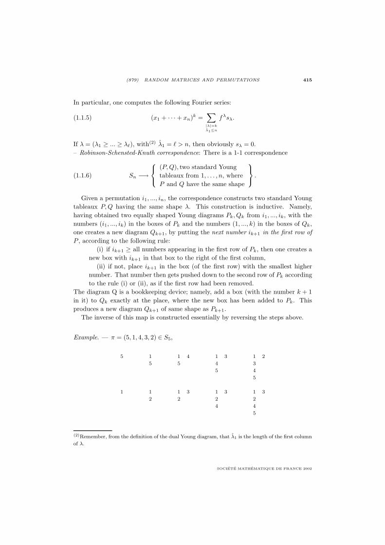
(879) RANDOM MATRICES AND PERMUTATIONS 415
In particular, one computes the following Fourier series:
(1.1.5) (x1 + · · ·+ xn)k =∑|λ|=k
λ1≤n
fλsλ.
If λ = (λ1 ≥ ... ≥ λ), with(2) λ1 = > n, then obviously sλ = 0.– Robinson-Schensted-Knuth correspondence: There is a 1-1 correspondence
(1.1.6) Sn −→
⎧⎨⎩(P, Q), two standard Youngtableaux from 1, . . . , n, whereP and Q have the same shape
⎫⎬⎭ .
Given a permutation i1, ..., in, the correspondence constructs two standard Youngtableaux P, Q having the same shape λ. This construction is inductive. Namely,having obtained two equally shaped Young diagrams Pk, Qk from i1, ..., ik, with thenumbers (i1, ..., ik) in the boxes of Pk and the numbers (1, ..., k) in the boxes of Qk,one creates a new diagram Qk+1, by putting the next number ik+1 in the first row ofP , according to the following rule:
(i) if ik+1 ≥ all numbers appearing in the first row of Pk, then one creates anew box with ik+1 in that box to the right of the first column,
(ii) if not, place ik+1 in the box (of the first row) with the smallest highernumber. That number then gets pushed down to the second row of Pk accordingto the rule (i) or (ii), as if the first row had been removed.
The diagram Q is a bookkeeping device; namely, add a box (with the number k + 1in it) to Qk exactly at the place, where the new box has been added to Pk. Thisproduces a new diagram Qk+1 of same shape as Pk+1.
The inverse of this map is constructed essentially by reversing the steps above.
Example. — π = (5, 1, 4, 3, 2) ∈ S5,
5 1 1 4 1 3 1 2
5 5 4 3
5 4
5
1 1 1 3 1 3 1 3
2 2 2 2
4 4
5
(2)Remember, from the definition of the dual Young diagram, that λ1 is the length of the first column
of λ.
SOCIETE MATHEMATIQUE DE FRANCE 2002

416 P. VAN MOERBEKE
Hence
π −→ (P (π), Q(π)) =
⎛⎜⎜⎝⎛⎜⎜⎝
1 2345
⎞⎟⎟⎠ ,
⎛⎜⎜⎝1 3245
⎞⎟⎟⎠⎞⎟⎟⎠
and L5(π) = 2 = #columns of P or Q.
The Robinson-Schensted-Knuth correspondence has the following properties– π → (P, Q), then π−1 → (Q, P )– length (longest increasing subsequence of π) = # (columns in P )– length (longest decreasing subsequence of π) = # (rows in P )– π2 = I, then π → (P, P )– π2 = I, with k fixed points, then P has exactly k columns of odd length.
1.2. Plancherel measure, integrals over U(n) and Toeplitz matrices
A next set of ideas is due to Vershik & Kerov [40], Diaconis & Shashahani [13],Biane [9], Rains [33, 34], Baik & Rains [7]. For a nice state-of-the-art account, seeAldous & Diaconis [5]. The uniform probability measure (see (1.1.1) for fλ) (1.0.1)on SN induces on Young diagrams, via the RSK bijection (1.1.6), the “Plancherel”probability measure
(1.2.1) PN (λ) =(fλ)2
N !, |λ| = N,
and so from (1.2.1) and the RSK bijection, one deduces a number of formulae below;notice, equality (ii) follows from (1.1.1) and (iii) follows from (i) and (1.1.5):
PN (L(πN ) ≤ n) =1
N !#
(P, Q), standard Young tableaux each ofarbitrary shape λ, with |λ| = N, λ1 ≤ n
(i)=
1N !
∑|λ|=Nλ1≤n
(fλ)2 =1
N !
∑|λ|=N
λ1≤n
(fλ)2, by duality of Young diagrams
(ii)= N !
n∑m=1
1m!
∑h∈Zm,hi≥1
hj=N+ m(m−1)
2
∏1≤i<j≤m
(hi − hj)2m∏1
1hj !2
(1.2.2)
(iii)=
1N !
∑|λ|=|µ|=N
λ1,µ1≤n
fλfµ〈sλ, sµ〉
=1
N !〈(x1 + · · ·+ xn)N , (x1 + · · ·+ xn)N 〉
(iv)=
1N !
∫U(n)
| trM |2NdM
ASTERISQUE 276
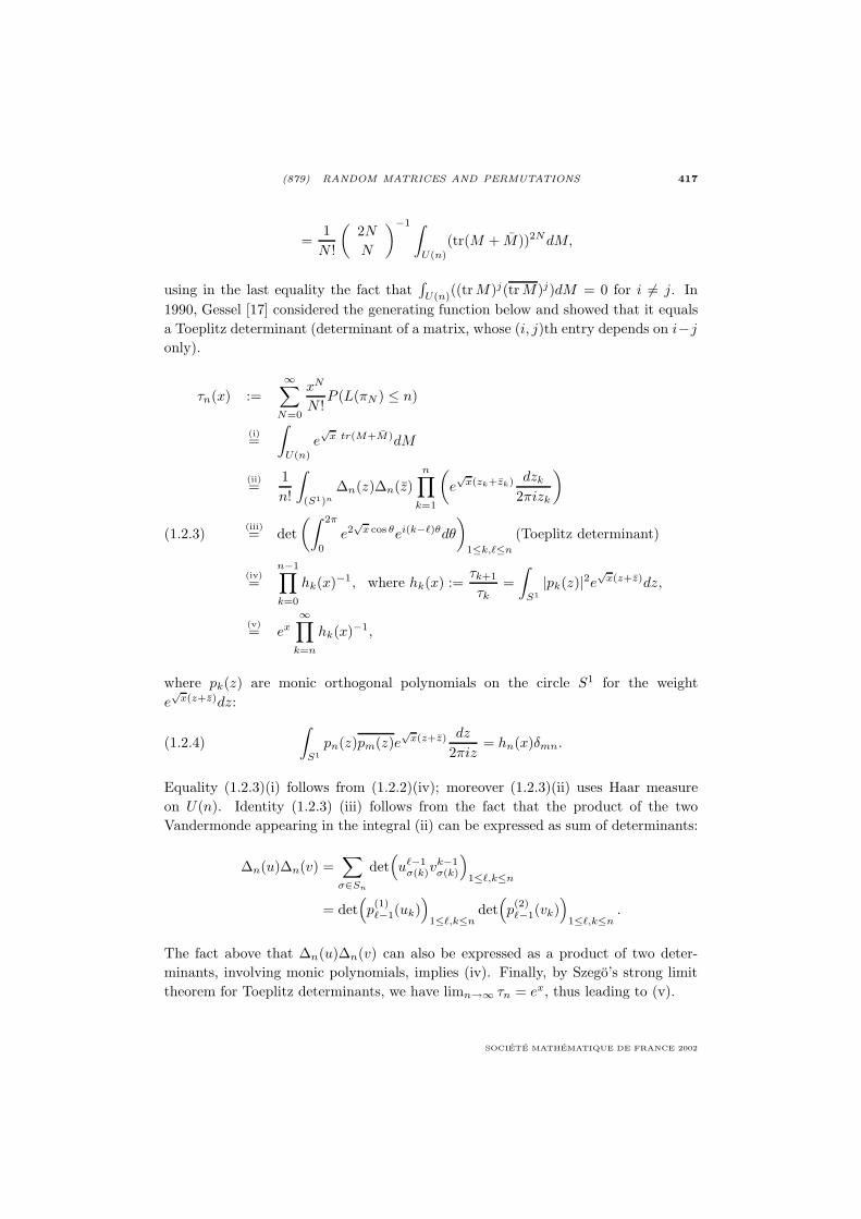
(879) RANDOM MATRICES AND PERMUTATIONS 417
=1
N !
(2N
N
)−1 ∫U(n)
(tr(M + M))2NdM,
using in the last equality the fact that∫
U(n)((tr M)j(tr M)j)dM = 0 for i = j. In
1990, Gessel [17] considered the generating function below and showed that it equalsa Toeplitz determinant (determinant of a matrix, whose (i, j)th entry depends on i−j
only).
τn(x) :=∞∑
N=0
xN
N !P (L(πN ) ≤ n)
(i)=∫
U(n)
e√
x tr(M+M)dM
(ii)=
1n!
∫(S1)n
∆n(z)∆n(z)n∏
k=1
(e√
x(zk+zk) dzk
2πizk
)(iii)= det
(∫ 2π
0
e2√
x cos θei(k−)θdθ
)1≤k,≤n
(Toeplitz determinant)(1.2.3)
(iv)=
n−1∏k=0
hk(x)−1, where hk(x) :=τk+1
τk=∫
S1|pk(z)|2e
√x(z+z)dz,
(v)= ex
∞∏k=n
hk(x)−1,
where pk(z) are monic orthogonal polynomials on the circle S1 for the weighte√
x(z+z)dz:
(1.2.4)∫
S1pn(z)pm(z)e
√x(z+z) dz
2πiz= hn(x)δmn.
Equality (1.2.3)(i) follows from (1.2.2)(iv); moreover (1.2.3)(ii) uses Haar measureon U(n). Identity (1.2.3) (iii) follows from the fact that the product of the twoVandermonde appearing in the integral (ii) can be expressed as sum of determinants:
∆n(u)∆n(v) =∑
σ∈Sn
det(u−1
σ(k)vk−1σ(k)
)1≤,k≤n
= det(p(1)−1(uk)
)1≤,k≤n
det(p(2)−1(vk)
)1≤,k≤n
.
The fact above that ∆n(u)∆n(v) can also be expressed as a product of two deter-minants, involving monic polynomials, implies (iv). Finally, by Szego’s strong limittheorem for Toeplitz determinants, we have limn→∞ τn = ex, thus leading to (v).
SOCIETE MATHEMATIQUE DE FRANCE 2002

418 P. VAN MOERBEKE
1.3. Virasoro constraints, integrable systems and Painleve V equation
Theorem 1.1. — For every ≥ 0, the Gessel generating function∞∑
N=0
xN
N !P (L(πN ) ≤ ) =
∫U()
e√
x tr(M+M)dM(1.3.1)
= exp∫ x
0
log(x
u
)g(u)du,
where g is the unique solution to the initial value problem:
(1.3.2)
⎧⎪⎪⎪⎪⎨⎪⎪⎪⎪⎩g′′ − g′2
2
(1
g − 1+
1g
)+
g′
u+
2u
g(g − 1)− 2
2u2
g − 1g
= 0
g(u) = 1− u
(!)2+ O(u+1), near u = 0. (Painleve V).
Theorem 1.1 is due to Hisakado [19], Tracy-Widom [36], by methods of functionalanalysis and Adler-van Moerbeke [3], by integrable methods. A similar statementholds for the set S0
2n of fixed-point free involutions π0(i.e., (π0)2 = I and π0(k) = k
for 1 ≤ k ≤ 2n). Put the uniform distribution on S02n :
(1.3.3) P (π02n) =
1(2n− 1)!!
=2nn!(2n)!
.
Then, in the following statement, due to Adler-van Moerbeke [3] and Baik-Rains [7],O(n)± refers to orthogonal matrices, with determinant = ±1 .
Theorem 1.2. — The generating function
2∞∑
k=0
(x2/2)k
k!P (L(π0
2k) ≤ + 1) = EO(+1)−ex trM + EO(+1)+ex trM
= exp(∫ x
0
f− (u)u
du
)+ exp(∫ x
0
f+ (u)u
du
),(1.3.4)
where f = f± is the unique solution to the initial value problem:
(1.3.5)
⎧⎪⎪⎪⎨⎪⎪⎪⎩f ′′′ +
1u
f ′′ +6u
f ′2 − 4u2
ff ′ − 16u2 + 2
u2f ′ +
16u
f +2(2 − 1)
u= 0
f± (u) = u2 ± u+1
!+ O(u+2), near u = 0. (Painleve V)
Proof of Theorem 1.1. — A brief outline will be given here, because of its interestingconnection with an integrable system, called the Toeplitz lattice (see [3]). Insertingtimes ti, with i = ...,−2,−1, 0, 1, 2, ..., and t0 = 0, in the integrals (1.2.3)(ii) over(S1)n, one obtains, setting t := (..., t−1, t0, t1, ...):
(1.3.6) In(t) =∫
(S1)n
|∆n(z)|2n∏
k=1
e
i=0 tizik
dzk
2πizk, n ≥ 0.
ASTERISQUE 276

(879) RANDOM MATRICES AND PERMUTATIONS 419
Virasoro constraints [3]. — The In’s satisfy a set of three linear partial differentialequations, forming an sl(2,Z)-algebra (Virasoro constraints), explicitly given by thethree equations:
(1.3.7)
⎛⎝ ∑i=∓1,0
(i± 1)ti±1∂
∂ti+ n
(t±1 +
∂
∂t∓1
)⎞⎠ In(t) = 0
and
⎛⎝∑i=0
iti∂
∂ti
⎞⎠ In(t) = 0.
Toeplitz lattice. — The t-dependent semi-infinite moment matrix,
(1.3.8) mn(t) :=(〈zk, z〉t
)0≤k,≤n−1
=(∮
S1
ρ(z)dz
2πizzk−e
i=0(tiz
i)
)0≤k,≤n−1
is a Toeplitz matrix and satisfies the simple differential equations:
(1.3.9)∂µij
∂tk= µi+k,j ,
∂µij
∂t−k= µi,j+k, for k ≥ 1.
In analogy with (1.2.3)(iii), define τn(t), instead of τn(x):
τn(t) := detmn(t).
The Borel factorization m∞(t) = S−11 (t)S2(t) with a lower-triangular matrix S1 (with
1’s along the diagonal) and an upper-triangular matrix S2, enables one to define(3)
L1 := S1ΛS−11 and L2 := S2ΛS−1
2 , which combined with the Toeplitz nature ofm∞ has a peculiar “rank 2”-structure, where xi and yi are certain integrals over U(n)and where hi = τi+1/τi, hi/hi−1 = 1− xiyi, h := diag(h0, h1, ...) and x0 = y0 = 1 :
L1 = h
⎛⎜⎜⎜⎜⎜⎜⎝−x1y0 1− x1y1 0 0−x2y0 −x2y1 1− x2y2 0−x3y0 −x3y1 −x3y2 1− x3y3
−x4y0 −x4y1 −x4y2 −x4y3
. . .
⎞⎟⎟⎟⎟⎟⎟⎠h−1
and
(1.3.10) L2 =
⎛⎜⎜⎜⎜⎜⎜⎝−x0y1 −x0y2 −x0y3 −x0y4
1− x1y1 −x1y2 −x1y3 −x1y4
0 1− x2y2 −x2y3 −x2y4
0 0 1− x3y3 −x3y4
. . .
⎞⎟⎟⎟⎟⎟⎟⎠ .
(3)where Λ is the shift matrix (Λv)n = vn+1, n ≥ 0, i.e., Λ is the semi-infinite matrix with all 0
entries, except for 1’s just above the diagonal.
SOCIETE MATHEMATIQUE DE FRANCE 2002
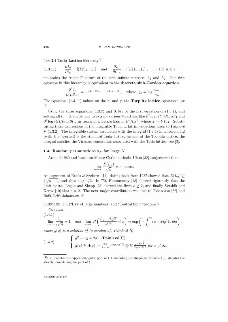
420 P. VAN MOERBEKE
The 2d-Toda Lattice hierarchy(4)
(1.3.11)∂Li
∂tn= [(Ln
1 )+ , Li] and∂Li
∂t−n= [(Ln
2 )− , Li] , i = 1, 2, n ≥ 1,
maintains the “rank 2” nature of the semi-infinite matrices L1 and L2. The firstequation in this hierarchy is equivalent to the discrete sinh-Gordon equation
∂2qn
∂t1∂t−1= −eqn−qn−1 + eqn+1−qn , where qn = log
τn+1
τn.
The equations (1.3.11) induce on the xi and yi the Toeplitz lattice equations; see[3].
Using the three equations (1.3.7) and ∂/∂t1 of the first equation of (1.3.7), andsetting all ti = 0, enable one to extract various t-partials, like ∂2 log τ(t)/∂t−1∂t1 and∂2 log τ(t)/∂t−2∂t1, in terms of pure partials in ∂k/∂xk, where x = t1t−1. Substi-tuting these expressions in the integrable Toeplitz lattice equations leads to PainleveV (1.3.2). The integrable system associated with the integral (1.3.4) in Theorem 1.2(with ti’s inserted) is the standard Toda lattice, instead of the Toeplitz lattice; theintegral satisfies the Virasoro constraints associated with the Toda lattice; see [3].
1.4. Random permutations πN for large N
Around 1960 and based on Monte-Carlo methods, Ulam [38] conjectured that
limn→∞
E(Ln)√n
= c exists.
An argument of Erdos & Szekeres [14], dating back from 1935 showed that E(Ln) ≥12
√n− 1, and thus c ≥ 1/2. In ’72, Hammersley [18] showed rigorously that the
limit exists. Logan and Shepp [23] showed the limit c ≥ 2, and finally Vershik andKerov [40] that c = 2. The next major contribution was due to Johansson [22] andBaik-Deift-Johansson [6]:
Theorem 1.3 (“Law of large numbers” and “Central limit theorem”)One has:
(1.4.1)
limn→∞
Ln
2√
n= 1, and lim
n→∞P
(Ln − 2
√n
n1/6≤ x
)= exp(−∫ ∞
x
(u− x)g2(u)du
),
where g(x) is a solution of (a version of) Painleve II,
(1.4.2)
⎧⎨⎩ g′′ = xg + 2g3 (Painleve II)
g(x) ∼= A(x) :=∫∞−∞ eixy−y3/3dy ∼= e− 2
3 x32
2√
πx1/4 for x ∞.
(4)( )+ denotes the upper-triangular part of ( ), including the diagonal, whereas ( )− denotes the
strictly lower-triangular part of ( ).
ASTERISQUE 276
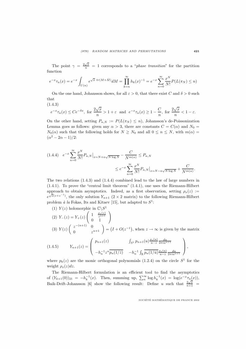
(879) RANDOM MATRICES AND PERMUTATIONS 421
The point γ = 2√
xn = 1 corresponds to a “phase transition” for the partition
function
e−xτn(x) = e−x
∫U(n)
e√
x tr(M+M)dM =∞∏
k=n
hk(x)−1 = e−x∞∑
n=0
xN
N !P (L(πN ) ≤ n)
On the one hand, Johansson shows, for all ε > 0, that there exist C and δ > 0 suchthat(1.4.3)
e−xτn(x) ≤ Ce−δx, for2√
x
n> 1 + ε and e−xτn(x) ≥ 1− C
n, for
2√
x
n< 1− ε.
On the other hand, setting Pn,N := P (L(πN ) ≤ n), Johansson’s de-PoissonizationLemma goes as follows: given any α > 3, there are constants C = C(α) and N0 =N0(α) such that the following holds for N ≥ N0 and all 0 ≤ n ≤ N , with m(α) =(α2 − 2α− 1)/2:
(1.4.4) e−x∞∑
n=0
xN
N !Pn,N
∣∣x=N+α
√N log N
− C
Nm(α)≤ Pn,N
≤ e−x∞∑
n=0
xN
N !Pn,N
∣∣x=N−α
√N log N
+C
Nm(α).
The two relations (1.4.3) and (1.4.4) combined lead to the law of large numbers in(1.4.1). To prove the “central limit theorem” (1.4.1), one uses the Riemann-Hilbertapproach to obtain asymptotics. Indeed, as a first observation, setting ρx(z) :=e√
x(z+z−1), the only solution Yn+1 (2 × 2 matrix) to the following Riemann-Hilbertproblem a la Fokas, Its and Kitaev [15], but adapted to S1:
(1) Y (z) holomorphic in C\S1
(2) Y−(z) = Y+(z)
(1 ρx(z)
zn+1
0 1
)(3) Y (z)
(z−(n+1) 00 zn+1
)=(I + O(z−1
), when z →∞ is given by the matrix
(1.4.5) Yn+1(z) =
⎛⎜⎝ pn+1(z)∫
S1 pn+1(u)ρx(u)u−z
du2πiun+1
−h−1n znpn(1/z) −h−1
n
∫R pn(1/u)ρx(u)
u−zdu
2πiun+1
⎞⎟⎠ ,
where pk(z) are the monic orthogonal polynomials (1.2.4) on the circle S1 for theweight ρx(z)dz.
The Riemann-Hilbert formulation is an efficient tool to find the asymptoticsof (Yk+1(0))21 = −h−1
k (x). Then, summing up,∑∞
n log h−1k (x) = log(e−xτn(x)),
Baik-Deift-Johansson [6] show the following result: Define u such that 2√
xn+1 =
SOCIETE MATHEMATIQUE DE FRANCE 2002

422 P. VAN MOERBEKE
1 − u21/3(n+1)2/3 , with −M < u < M for a given M > 0. Then the estimate below
holds, where g is the solution to (1.4.2):∣∣∣∣log(e−xτn(x)) −∫ ∞
u
2if(y)dy
∣∣∣∣ = C(M)n1/3
+ Ce−1/4M3/2
with 2if(y) = −∫∞y g2(α)dα. This estimate combined with Johansson’s de-
Poissonization Lemma leads to (1.4.1) and (1.4.2).
2. THE SPECTRUM OF RANDOM MATRICES
Random matrix theory deals with an ensemble of matrices M , having some symme-try condition to guarantee the reality of the spectrum, e.g., the Hermitian ensembleHn, the symmetric ensemble Sn or the symplectic ensemble T2n. Define a probabilitymeasure, based on a Haar measure, which in “polar coordinates” is expressed in termsof the Vandermonde with a power β:
cne−trV (M)dM = cn|∆n(z)|βn∏1
e−V (zk)dzkdU,
with V ′ = gf rational, dM = Haar measure. The three ensembles Hn, Sn, T2n appear
very naturally as the tangent spaces (at the identity) to the simplest symmetric spaces:
non-compact = ⊕ with space Haar
symmetric =tangent space = M ∈ , with... measure
space G/K to G/K at I on
SL(n, )/SU(n) sl(n, ) = su(n) ⊕Hn M = M β = 2
SL(n,)/SO(n) sl(n,) = so(n) ⊕ Sn M = M β = 1
SU∗(2n)/USp(n) su∗(2n) = (sp(n, ) ∩ u(2n)) ⊕ T2n M = M, M = JMJ−1 β = 4
Question. — What is the statistics of the spectrum of M ?
For Hn and Sn, if the probability P (M ∈ dM) satisfies the following two require-ments: (i) invariance under conjugation by unitary transformations M → UMU−1,(ii) the random variables Mii, !Mij , "Mij , 1 ≤ i < j ≤ n are independent, thenV (z) is quadratic (Gaussian ensemble) ([28]).
2.1. Virasoro constraints, Toda and Pfaff lattices and KP equations
Consider weights of the form ρ(z)dz := e−V (z)dz on an interval F = [A, B] ⊆ R,with rational logarithmic derivative and subjected to the following boundary condi-tions:
(2.1.1) −ρ′
ρ=
g
f=∑∞
0 bizi∑∞
0 aizi, lim
z→A,Bf(z)ρ(z)zk = 0 for all k ≥ 0,
and a disjoint union of intervals E =⋃2r
1 [x2i−1, x2i] ⊂ F ⊂ R.
ASTERISQUE 276

(879) RANDOM MATRICES AND PERMUTATIONS 423
Theorem 2.1 (Adler-van Moerbeke [1])The vector of integrals I(t, x; β) = (I0 = 1, I1(t, x; β), ...), with t := (t1, t2, ...) and
x := (x1, ..., x2r) and
(2.1.2) In(t, x; β) :=∫
En
|∆n(z)|βn∏
k=1
(e∞
1 tizikρ(zk)dzk
)for n > 0
satisfies the following Virasoro constraints(5) for all k ≥ −1:⎛⎝− 2r∑1
xk+1i f(xi)
∂
∂xi+∑i≥0
(ai
βJ(2)k+i(t, n)− bi
βJ(1)k+i+1(t, n)
)⎞⎠ I(t, x; β) = 0,
in terms of the coefficients ai, bi of the rational function (− log ρ)′ and the end pointsxi of the subset E, as in (2.1.1). The βJ(2)
k and βJ(1)k form a Virasoro and a
Heisenberg algebra respectively, interacting as follows[βJ(2)
k , βJ(2)
]= (k − ) βJ(2)
k+ + c
(k3 − k
12
)δk,−[
βJ(2)k , βJ(1)
]= − βJ(1)
k+ + c′k(k + 1)δk,−.[βJ(1)
k , βJ(1)
]=
k
βδk,−,(2.1.3)
with central charge c = 1− 6
((β
2
)1/2
−(
β
2
)−1/2)2
and c′ =(
1β− 1
2
).
Moreover:(i) τn(t) := 1
n!In(t, x, β)|β=2 form the τ-functions of the standard Toda lattice; inparticular, each τn satisfies the KP equation:((
∂
∂t1
)4
+ 3(
∂
∂t2
)2
− 4∂2
∂t1∂t3
)log τn + 6
(∂2
∂t21log τn
)2
= 0.
(ii) τ2n(t) :=
⎧⎪⎨⎪⎩1
(2n)! I2n(t, x; β)|β=1
1n! In(2t, x; β)|β=4
form the τ-functions of the Pfaff lattice (i.e.,
they are Pfaffians, rather than determinants); in particular, they satisfy the Pfaff-KPequation:
((∂
∂t1
)4
+ 3(
∂
∂t2
)2
− 4∂2
∂t1∂t3
)log τ2n + 6
(∂2
∂t21log τ2n
)2
= 12τ2n−2τ2n+2
τ22n
.
(5)When E equals the whole range F , then the ∂/∂xi’s are absent in the formulae (2.1.7).
SOCIETE MATHEMATIQUE DE FRANCE 2002

424 P. VAN MOERBEKE
2.2. The Gaussian ensemble: PDE’s for the statistics of the spectrum
Theorem 2.2. — For the Gaussian ensemble, the probabilities(6): (β = 2, 1, 4)
Pn(E) := Pn( all spectral points of M ∈ E)
=
∫Hn(E), Sn(E) or Tn(E) e−tr M2
dM∫Hn(R), Sn(R) or Tn(R)
e−tr M2dM(2.2.1)
=
∫En |∆n(z)|β
∏nk=1 e−z2
kdzk∫Rn |∆n(z)|β
∏nk=1 e−z2
kdzk
satisfy the following PDE’s in the xi’s (Bk =∑2r
1 xk+1i
∂∂xi
, δβ1,4 = 1 for β = 1, 4 and
0 otherwise, fn(x) = ddx log Pn):(7)
δβ1,4Q
(Pn− 2
1Pn+ 2
1
P 2n
− 1
) 2 and n even, for β = 11 and n arbitrary, for β = 4
=
⎧⎪⎪⎪⎪⎨⎪⎪⎪⎪⎩
(B4−1 + (Q2 + 6B2
−1F )B2−1 + (2 − δβ
1,4)4β
(3B20 − 4B−1B1 + 6B0)
)log Pn
for E =⋃2r
1 [x2i−1, x2i]
f ′′′n + 6f ′2
n +(
4x2
β(δβ
1,4 − 2) + Q2
)f ′
n −4x
β(δβ
1,4 − 2)fn, for E = [−∞, x].
Note that for β = 2 and for E = [−∞, x], the equation above takes on the simpleform:
(2.2.2) f ′′′n + 6f ′2
n + 8nf ′n + 4xfn = 0. (Painleve IV)
Equation (2.2.2) was obtained by Tracy-Widom [35] and the rest of Theorem 2.2is due to M. Adler, T. Shiota and P. van Moerbeke ([4] and [1]).
2.3. Infinite Hermitian matrix ensembles
Consider probability (2.2.1) for β = 2 and let the size n of the matrices go to ∞.To perform this limit, one uses a different representation; namely,
(2.3.1) Pn(E) :=
∫Hn(E)
e−tr M2dM∫
Hne−tr M2dM
=1n!
∫En
det(Kn(zk, z))1≤k,≤n
n∏1
ρ(dzi),
(6)Hn(E), Sn(E) or Tn(E) denotes the subset of matrices with spectrum in E ⊆ .(7)Also, define the invariant polynomials
Q = 12n
n + 1 − 2
β
and Q2 = 4(1 + δβ
1,4)
2n + δβ
1,4(1 − 2
β)
.
ASTERISQUE 276
(879) RANDOM MATRICES AND PERMUTATIONS 425
can be represented in terms of a reproducing kernel(2.3.2)
Kn(y, z) :=n∑
j=1
pj−1(y)√hj−1
pj−1(z)√hj−1
, where∫
RKn(y, z)Kn(z, u)ρ(dz) = Kn(y, u).
The reproducing property follows from the orthogonality of the monic orthogonalpolynomials pk = pk(z) for the Gaussian weight e−z2
dz on R, and the L2-normshk =∫
R p2k(z)e−z2
dz of the pk’s. We also have the following Fredholm determinantformula
P (exactly k eigenvalues ∈ [x1, x2])
=(−1)k
k!
(∂
∂λ
)k
det(I − λKn(y, z)I[x1,x2](z))
∣∣∣∣∣λ=1
.
When the size n of the Hermitian matrices tends to ∞, the following holds:
– Wigner’s semi-circle law: For this ensemble and for very large n, the density ofeigenvalues tends to the semi-circle distribution on the interval [−
√2n,√
2n].– Bulk scaling limit: From the formula above, it follows that the average number
of eigenvalues per unit length near z = 0 (“the bulk”) is given by√
2n/π and thusthe average distance between two consecutive eigenvalues is given by π/
√2n. Upon
using this rescaling, one shows ([24, 27, 29, 32, 21])
limn∞
π√2n
Kn
(πy√2n
,πz√2n
)=
sin π(y − z)π(y − z)
=: K(y, z) (Sine kernel)
with
(2.3.3) P (no eigenvalues ∈ [0, x]) = det(I −K(y, z)I[0,x](z)) = exp∫ πx
0
f(x)x
dx,
where f(x, λ) is a solution to the Painleve V differential equation, (see Jimbo, Miwa,Mori, Sato [21]), (′ = ∂/∂x)
(xf ′′)2 − 4(xf ′ − f)(−f ′2 − xf ′ + f) = 0 with f(x; λ) ∼= −x
π, for x 0.
– Edge scaling limit: I will particularly concentrate on the “edge”√
2n of theWigner semi-circle. There the scaling is
√2n1/6, which makes the problems consider-
ably subtler; this will be used in (2.3.7) (see [10, 16, 28, 35]). The main result can bestated as follows:
Theorem 2.3. — Given the spectrum z1 ≥ z2 ≥ ... of the large random Hermitianmatrix M , define the “eigenvalues” in a new scale:
(2.3.4) ui = 2n23
(zi√2n− 1)
for n∞
SOCIETE MATHEMATIQUE DE FRANCE 2002

426 P. VAN MOERBEKE
then the statistics of the largest “eigenvalue”u1 (in the new scale) is given by the sameprobability distribution as the length of the longest increasing sequence:
P (u1 ≤ x) = exp(−∫ ∞
x
(α− x)g2(α)dα
),
with
⎧⎨⎩ g′′ = xg + 2g3 (Painleve II)
g(x) ∼= A(x) ∼= − e− 23 x
32
2√
πx1/4 for x ∞.
(2.3.5)
More generally, P (no points ui ∈ [x1, x2]) satisfies the partial differential equation(2.3.6)(B3−1 − 4(B0 −
12))
f + 6(B−1f)2 = 0, with f :=2∑1
∂ log P
∂xi, Bk =
2∑1
xk+1 ∂
∂xi.
Tracy-Widom [35] have first obtained result (2.3.5) by methods of functional anal-ysis. In [4], equations (2.3.5) and (2.3.6) were derived using integrable systems andVirasoro constraints.Proof . — Setting z =
√2n + u√
2n1/6 , in the kernel Kn(x, y) of (2.3.2), one proves
(2.3.7) limn∞
1√2n1/6
Kn
(√2n +
u√2n1/6
,√
2n +v√
2n1/6
)= K(u, v),
where the Airy kernel K is defined in terms of the Airy function:
K(u, v) =∫ ∞
0
A(x + u)A(x + v)dx,
A(u) =∫ ∞
−∞eiux−x3/3dx ∼=
e−(2/3)u3/2
2√
πu1/4, for u ∞.
(2.3.8)
To find the differential equations (2.3.6), one proceeds (sketchily) as follows: as afirst step, notice that, setting L2 := ( ∂
∂t1)2 + q(t), t := (t1, t2, ...), the solution q(t)
and Ψ(t; z) (with asymptotics Ψ(t; z) = e∞
1 tizi
(1+O(z−1)), z ∈ C, z →∞) to theinitial value problem:
(2.3.9)
⎧⎪⎨⎪⎩(L2 − z2)Ψ(t; z) = 0, ∂L2
∂tn= [(Ln)+, L2], ∂Ψ
∂tn= (Ln)+Ψ,
q(t(0)) = −x, at t = t(0) := (x, 0, 23 , 0, 0, ...),
is given by Kontsevich’s integral (Z diagonal and N arbitrary), which itself is inti-mately related to the Airy function A(x),
(2.3.10)
⎧⎪⎪⎪⎨⎪⎪⎪⎩q(t) = 2
∂2
∂t21log τ(t),
Ψ(t; z) = e∞
1 tizi
τ(t− [z−1])/τ(t),Ψ(t(0); z) = z1/2A(x + z2) = exz+ 2
3 z3(1 + O(z−1)), z →∞.
ASTERISQUE 276

(879) RANDOM MATRICES AND PERMUTATIONS 427
with
τ(t) =
∫HN
dXe−tr(X3/3+X2Z)∫HN
dXe−tr(X2Z), tn := − 1
ntrZ−n +
23δn3
and[z−1] = (z−1, z−2/2, z−3/3, ...) ∈ C∞
These data define a kernel
(2.3.11) Kt(z2, z′2) :=1
z12 z′
12
∫ ∞
0
Ψ(t; z)Ψ(t; z′)dt1, where t = (t1, t2, ...)
which flows off the Airy kernel K(z2, z′2), defined in (2.3.8), upon using (2.3.10).Then, one shows that both, Kontsevich’s integral τ(t) and the product τ(t, E) :=
τ(t).det (I −Kt(λ, λ′)IE(λ′)), with E =
⋃2r1 [x2i−1, x2i] ⊂ R, satisfy Virasoro constraints,
of which the two first ones read (after the time shift t3 → t3 +2/3, in view of (2.3.9)):
2r∑i=1
∂
∂xilog τ(t, E) =
⎛⎝ ∂
∂t1+
12
∑i≥3
iti∂
∂ti−2
⎞⎠ log τ(t, E) +t214
2r∑i=1
xi
∂
∂xilog τ(t, E) =
⎛⎝ ∂
∂t3+
12
∑i≥1
iti∂
∂ti
⎞⎠ log τ(t, E) +116
,(2.3.12)
Both, τ(t) and τ(t, E), also satisfy the Korteweg-de Vries equation (KP equation,depending on odd ti’s only)
(2.3.13)
((∂
∂t1
)4
− 4∂2
∂t1∂t3
)log τ + 6
(∂2
∂t21log τ
)2
= 0. (KdV)
Differentiating (2.3.12) in t1 and t3, and setting all ti = 0 enable one to express thet-partials ∂2
∂t21log τ∣∣∣t=0
, ∂4
∂t41log τ∣∣∣t=0
, ∂2
∂t1∂t3log τ∣∣∣t=0
appearing in the KdV equation
in terms of partials ∂/∂xi.Setting these expressions in the the KdV -equation at t = 0, implies that the
statistics of the scaled eigenvalues ui (for the Airy kernel (2.3.8))
P (Ec) := P (all “eigenvalues”, ui ∈ Ec) = det(I −KIE) =τ(t, E)τ(t)
∣∣∣∣t=0
,
satisfies the partial differential equation (2.3.6) with
f :=2r∑1
∂ log P
∂xi, Bk =
2r∑1
xk+1 ∂
∂xi.
When E = (x,∞), the equation (2.3.6) for f = ∂ log P ((−∞, x])/∂x becomes a3rd order ODE (Chazy-type equation)
(2.3.14) f ′′′ − 4xf ′ + 2f + 6f ′2 = 0.
SOCIETE MATHEMATIQUE DE FRANCE 2002

428 P. VAN MOERBEKE
According to [12] , this equation has a first integral, which is a Painleve II equation
(2.3.15) f ′′2 + 4f ′(f ′2 − xf ′ + f) = 0.
and this equation has a solution given by f := g′2 − xg2 − g4 and f ′ = −g2, whichestablishes (2.3.5) and (2.3.6).
3. LARGE RANDOM MATRICES AND PERMUTATIONS: ADIRECT CONNECTION VIA ENUMERATIVE GEOMETRY
For large random Hermitian matrices, whose entries have Gaussian real and imag-inary part of variance = 1/2, the Wigner semi-circle has support on (−2
√n, 2√
n),instead of [−
√2n,√
2n]. Then the (slightly modified) scaling (2.3.4) is given by
(3.1) ui = n2/3( zi
2n1/2− 1)
for n ∞.
Given the set of partitions λ = (λ1 ≥ λ2 ≥ ...) of n, in view of (1.4.1), consider
(3.2) vi = n1/3
(λi
2n1/2− 1)
for n ∞.
Theorems 1.3 and 2.3 show that the variables u1 and v1 have the same probabilitydistribution. Okounkov [31] shows in a direct way that the joint distribution of all ui
and vi coincide; more specifically:
Theorem 3.1 (Okounkov, [31]). — For any m ≥ 1, any ξ1, ..., ξm > 0, the followingholds:
E(∞∑
i=1
eξ1ui ...
∞∑i=1
eξmui) = E(∞∑
i=1
eξ1vi ...
∞∑i=1
eξmvi), when n ∞.
The left hand side, which relates to random permutations, hinges on the followingexpressions:(
12√
n
)k1+...+km nm/2
n!tr(Xk1
1 )...Xkmm ))
=(
12
)k1+...+km∑S
n12 (χ(S)−m) |CovS(k1, ..., km)| ,
In this expression, the Xi are certain matrices, such that e.g. λj−j is an eigenvalue ofX1, if (j, λj) is a corner of the Young diagram (i.e., λj > λj+1). Also CovS(k1, ..., km)are coverings of S2 ramified according to a rule, given by the numbers k1, ..., km.
ASTERISQUE 276

(879) RANDOM MATRICES AND PERMUTATIONS 429
The right hand side relates to random matrices and has an interpretation as a“map” on a surface. It hinges on the following formula for M ∈ U(n):(
12√
n
)k1+...+km
E(tr(Mk1)...tr(Mkm ))
=(
12
)k1+...+km∑S
nχ(S)−m |MapS(k1, ..., km)| ,
where the sum is taken over all the homeomorphism classes of orientable, not neces-sarily connected surfaces S; χ(S) is its Euler number and MapS(k1, ..., km) denotesthe ways to cover the surface S with m polygons (a k1-gon, a k2-gon,..., a km-gon) bypairwise gluing the sides of different or the same ki-gons. Each polygon has a markedvertex, to distinguish a k-gon from its k − 1 rotations.
The main proposition, established by Okounkov and leading to Theorem 3.1, is thefollowing: for connected surfaces, as ki →∞,
CovS(k1, ..., km) ∼= MapS(k1, ..., km).
4. INTEGRALS, MOMENT MATRICES AND INTEGRABLESYSTEMS
The first column contains a list of matrix integrals and a Fredholm determinant.After perturbing the integral by inserting times ti’s and possibly si’s, the new in-tegral thus obtained satisfies linear PDE’s (Virasoro constraints). The integral canbe represented as a determinant of a “moment” matrix, (defined by an appropriateinner-product) or a Pfaffian, if the moment matrix is skew. Performing an appropriate“Borel factorization” of this associated moment matrix, one shows that each of theseintegrals, as a function of the ti and si’s, satisfies an integrable lattice or an integrablePDE. In all the cases, combining both systems of equations leads to ODE’s or PDE’sfor the corresponding integral, in x or in the boundary of E. The last column liststhe connection with probability. For more information on the 6th integral and thedouble matrix integral, see [37, 3, 2].
SOCIETE MATHEMATIQUE DE FRANCE 2002

430 P. VAN MOERBEKE
τ -functions satisfying = determinant underlying connecting with
Virasoro constraints, or Pfaffian of integrable
after inserting ti’s m of the form: lattice or PDEH(E)
e−trV (M)dM Hankel Toda lattice spectrum of random
Hermitian matrices
S(E)
e−trV (M)dM skew-symmetric Pfaff lattice spectrum of random
symmetric matrices
T(E)
e−trV (M)dM skew-symmetric Pfaff lattice spectrum of random
symplectic matrices
U()
e√
x tr(M+M)dM Toeplitz Toeplitz lattice longest increasing sequence
in random permutations
O()±
ex trMdM Hankel Toda lattice longest increasing sequence
in random involutions
U()
det(I + M)k Toeplitz Toeplitz lattice longest increasing sequence
e−xtrMdM in random words
detI − K(y, z)I(x,∞)(z)
Fredholm KdV equation spectrum of infinite
determinant random Hermitian matrices
(K sine or Airy kernel) (bulk or edge scaling limit)
H×H(E)
dM1dM2 general 2d-Toda lattice coupled random matrices
×e−tr(M21+M2
2−cM1M2)
ASTERISQUE 276
(879) RANDOM MATRICES AND PERMUTATIONS 431
REFERENCES
[1] M. Adler and P. van Moerbeke: Symmetric random matrices and the PfaffLattice, to appear in: Annals of Mathematics, sept 2000 (solv-int/9903009)and The Hermitian, symmetric and symplectic ensembles and PDE’s (math.-phys./009001).
[2] M. Adler and P. van Moerbeke: The spectrum of coupled random matrices,Annals of Mathematics, 149, 921–976 (1999).
[3] M. Adler and P. van Moerbeke: Integrals over classical groups, randompermutations, Toda and Toeplitz lattices, Comm. Pure Appl. Math. (2000)(math.CO/9912143).
[4] M. Adler, T. Shiota and P. van Moerbeke: Random matrices, vertex opera-tors and the Virasoro algebra, Phys. Lett. A 208, 101-112, (1995). And Randommatrices, Virasoro algebras and non-commutative KP, Duke Math. J. 94, 379-431(1998).
[5] D. Aldous and P. Diaconis: Longest increasing subsequences: From patiencesorting to the Baik-Deift-Johansson theorem, Bull. Am. Math. Soc. (new series)36 (4), 413–432 (1999).
[6] J. Baik, P. Deift and K. Johansson: On the distribution of the length of thelongest increasing subsequence of random permutations, Math. Archive, JournalAmer. Math. Soc. 12, 1119-1178 (1999) (math.CO/9810105).
[7] J. Baik and E. Rains: Algebraic aspects of increasing subsequences, (1999),math.CO/9905083
[8] D. Bessis, Cl. Itzykson and J.-B. Zuber : Quantum field theory techniques ingraphical enumeration, Adv. Appl. Math. 1, 109-157 (1980).
[9] P. Biane: Representations of symmetric groups and free probability, preprint(1998).
[10] M. Bowick and E. Brezin: Universal scaling of the tail of the density of eigen-values in random matrix models, Phys. Letters B 268, 21–28 (1991).
[11] S. Chadha, G. Mahoux, M.L. Mehta : A method of integration over matrixvariables : II, J. Phys. A: Math. Gen. 14, 579-586 (1981).
[12] C.M. Cosgrove: Chazy classes IX-XII of third-order differential equations,Stud. Appl. Math. 104, 3, 171-228 (2000).
[13] P. Diaconis, M. Shashahani: On the eigenvalues of random matrices J. Appl.Prob., suppl. in honour of Takacs 31A, 49-61 (1994).
[14] P. Erdos and G. Szekeres: A combinatorial theorem in geometry, CompositioMath., 2, 463–470 (1935).
[15] A.S. Fokas, A.R. Its, A.V. Kitaev: The isomonodromy approach to matrixmodels in 2d quantum gravity, Comm. Math. Phys., 147, 395–430 (1992).
SOCIETE MATHEMATIQUE DE FRANCE 2002

432 P. VAN MOERBEKE
[16] P.J. Forrester: The spectrum edge of random matrix ensembles, Nucl. Phys.B, (1993).
[17] I. M. Gessel: Symmetric functions and P-recursiveness, J. of Comb. Theory,Ser A, 53, 257–285 (1990).
[18] J.M. Hammersley: A few seedlings of research, Proc. Sixth. Berkeley Symp.Math. Statist. and Probability, Vol. 1, 345–394, University of California Press(1972).
[19] M. Hisakado: Unitary matrix models and Painleve III, Mod. Phys. Letters, A11 3001–3010 (1996).
[20] Cl. Itzykson, J.-B. Zuber: The planar approximation, J. Math. Phys. 21,411–421 (1980).
[21] M. Jimbo, T. Miwa, Y. Mori and M. Sato: Density matrix of an impenetrableBose gas and the fifth Painleve transcendent, Physica 1D, 80–158 (1980).
[22] K. Johansson: The Longest Increasing Subsequence in a Random Permutationand a Unitary Random Matrix Model, Math. Res. Lett., 5, no. 1-2, 63–82 (1998).
[23] B.F. Logan and L.A. Shepp: A variational problem for random Young tableaux,Advances in Math., 26, 206–222 (1977).
[24] R.D. Kamien, H.D. Politzer, M.B. Wise: Universality of random-matrix pre-dictions for the statistics of energy levels Phys. rev. letters 60, 1995–1998 (1988).
[25] M. Kontsevich: Intersection theory on the moduli space of curves and thematrix Airy function, Comm. Math. Phys. 147, 1-23 (1992).
[26] D. Knuth: “The Art of Computer programming, Vol III: Searching and Sorting”,Addison-Wesley, Reading, MA, 1973.
[27] G. Mahoux, M.L. Mehta: A method of integration over matrix variables: IV,J. Phys. I (France) 1, 1093–1108 (1991).
[28] M.L. Mehta: Random matrices, 2nd ed. Boston: Acad. Press, 1991.[29] T. Nagao, M. Wadati: Correlation functions of random matrix ensembles re-
lated to classical orthogonal polynomials, J. Phys. Soc of Japan, 60 3298–3322(1991).
[30] A.M. Odlyzko: On the distribution of spacings between the zeros of the zetafunction 48, 273-308 (1987).
[31] A. Okounkov: Random matrices and random permutations (1999), math.CO/9903176
[32] L.A. Pastur: On the universality of the level spacing distribution for some en-sembles of random matrices, Letters Math. Phys., 25 259–265 (1992).
[33] E. M. Rains: Topics in Probability on compact Lie groups, Harvard Universitydoctoral dissertation, (1995).
5B[34] E. M. Rains: Increasing subsequences and the classical groups, Elect. J. of Com-
binatorics, 5, R12 (1998).
ASTERISQUE 276

(879) RANDOM MATRICES AND PERMUTATIONS 433
[35] C.A. Tracy and H. Widom: Level-Spacings distribution and the Airy kernel,Commun. Math. Phys., 159, 151–174 (1994).
[36] C.A. Tracy and H. Widom: Random unitary matrices, permutations andPainleve (1999), math.CO/9811154
[37] C.A. Tracy and H. Widom: On the distribution of the lengths of the longestmonotone subsequences in random words (1999), math.CO/9904042
[38] S.M. Ulam: Monte Carlo calculations in problems of mathematical physics, inModern Mathematics for the Engineers, E.F. Beckenbach ed., McGraw-Hill, 261–281 (1961).
[39] P. van Moerbeke: Integrable lattices: random matrices and permutations,MSRI-volume on Random matrices and exactly solvable models, Eds.: P. Bleher,A. Its, Oxford University press, 2000 (math.CO/00-10).
[40] A.M. Vershik and S.V. Kerov: Asymptotics of the Plancherel measure of thesymmetric group and the limiting form of Young tableaux, Soviet Math. Dokl.,18, 527–531 (1977).
Pierre VAN MOERBEKE
Departement de MathematiquesUniversite de LouvainB–1348 Louvain-la-Neuve (Belgium)E-mail : [email protected]
andBrandeis UniversityWaltham, Mass 02454, USAE-mail : [email protected]
SOCIETE MATHEMATIQUE DE FRANCE 2002


!
"! # $ ## % & # $ '(' % ) *+ * ,* #$,* * +*# # %
- " . # % !
" #$%$$&' */ . ,*. % (! " * . - % % ! "!- /-'.$ % ()
* +)
" 0,*# $ #( % $, - *) *
,0 % . /! / 0 !& 1' % )* 1$ * )*& - -.*#2 2 % & 0 234
) , * % 5* 6) 7 ) )-
8 (+ % 0 $345 6 3 738 97:;5< 6< : =>::4 9=945: ';97 4;7
0-? . #, 3 "!, + ,, 2 9534
' ,# + % . % &)) - ) 7 !
34634 #>47 @ 3 99535: "! '* -- -' ;:9
+' 9534 "!. - % !
." 9&$$ ." .:;$.' 0 - % <) * ) ##/#2 ' *-#' % & ," *-- $ *# % . GL(n) (( = +
) $ % (! , ! )* )
. )

) !& A4 3 4;43535: 9 5:3 9 >;34 A4: .+ 9534 , ## -$( % /6) !
$" >$3/$3'& . ,* . #,*#,* % * !
& . , -2 % () !)) p*& $ . % ! ! ! Lp p
& ( # ( (,* % q *4 *
& !)&&& "! # % # &) - -00 $ % / ? &?0& 1 % 0@ 6 ) & !
& B ## - 2/ % 6 !
) "!- (' % / ) )!) ) )) 0 '-= .$ % ) ) =
1! ) ))* )) & !&) *;C D . + 3 " () "!. #- % . )- 1 !)) +) )& $# % $ )* /
)) 2 ". + % : !) 6:3 ;9;:6 5: 4;34 ;CA4; E 4;: F) "!, + ,, 2 % 0 ! A) "!+ ,* % .! % L p* ) p* ,A5; :54537 :A4 3>47 5:;4 EG!+4H F )& !
K!3>47 E34;A4C F - % : + 8 8& . ,*. "!. ,*' % (, ) .459 p!;95< E5:;54 9 4 F , ;:;7356 3>9 5: 97:;56; 73 E. I;:54 F $ % F 4 ! # ** ' ", "#2 / $- % &) *
p p = p
* #*- % . - . )!


![[Frenkel.] Vertex Algebras (Bourbaki org](https://static.fdocuments.in/doc/165x107/577d24401a28ab4e1e9bfeba/frenkel-vertex-algebras-bourbaki-org.jpg)