Semi-parametric forecasting of Spikes in Electricity … forecasting of Spikes in Electricity Prices...

NCER Working Paper SeriesNCER Working Paper Series

Semi-parametric forecasting of Spikes in Electricity Prices

A E ClementsA E Clements J E FullerJ E Fuller A S Hurn A S Hurn Working Paper #82Working Paper #82 May 2012May 2012

Semi-parametric forecasting of Spikes in ElectricityPrices

A E Clements, J E Fuller and A S HurnSchool of Economics and Finance, Queensland University of Technology.

Abstract

The occurrence of extreme movements in the spot price of electricity represent asignificant source of risk to retailers. Electricity markets are often structured so as toallow retailers to purchase at an unregulated spot price but then sell to consumers ata heavily regulated price. As such, the ability to forecast price spikes is an importantaspect of effective risk management. A range of approaches have been consideredwith respect to modelling electricity prices, including predicting the trajectory of spotprices, as well as more recently, focusing of the prediction of spikes specifically. Thesemodels however, have relied on time series approaches which typically use restrictivedecay schemes placing greater weight on more recent observations. This paper devel-ops an alternative, semi-parametric method for forecasting that does not rely on thisconvention. In this approach, a forecast is a weighted average of historical price data,with the greatest weight given to periods that exhibit similar market conditions to thetime at which the forecast is being formed. Weighting is determined by comparingshort-term trends in electricity price spike occurrences across time, including otherrelevant factors such as load, by means of a multivariate kernel scheme. It is foundthat the semi-parametric method produces forecasts that are more accurate than thepreviously identified best approach for a short forecast horizon.

KeywordsElectricity Prices, Prices Spikes, Semi-parametric, Multivariate Kernel.

JEL classification numbersC14, C53.

Corresponding authorJoanne FullerSchool of Economics and FinanceQueensland University of TechnologyBrisbane, Qld 4001Australia

email: [email protected]

1 Introduction

In deregulated electricity markets, retailers buy electricity from a grid at a market price,known as the spot price, and sell electricity to consumers at a heavily regulated price. Spotprices in these markets are known to exhibit sudden and very large jumps to extreme pricelevels, due to stresses such as unexpected increases in demand, unexpected supply short-falls, and failure of transmission infrastructure (see, for example, Geman and Roncorni,2006). The spot prices remain at these levels before abruptly jumping back down to thenormal trading range upon resolution of the stress. These “extreme price events”, also re-ferred to as “price spikes”, are particularly hazardous to electricity retailers who cannot passon price risk to customers (Anderson, et al., 2006). Improving the understanding of factorscontributing to the occurrence of extreme price events, as well as accurately forecastingthese events, is important for risk management in the energy sector.

In the mid 1990s, the regional electricity markets of New South Wales, Queensland, Victo-ria, South Australia, and the Australian Capital Territory were merged to form the NationalElectricity Market (NEM) in Australia. These markets were linked using large capacitytransmission lines, with the exception of Queensland, which participated under the NEMmarket rules but was not physically connected to the NEM until February 2001. The NEMoperates as a pooled market in which all available supply to a region is aggregated andgenerators are dispatched so as to satisfy demand as cost effectively as possible. If, in anygiven region, local demand exceeds local supply or electricity in a neighbouring region issufficiently inexpensive to warrant transmission, then electricity is imported and exportedbetween regions subject to the physical constraints of the transmission infrastructure. Interms of composition of the supply side, coal-fired generators and hydroelectric productionhave a low marginal cost of production supplying respectively 84% and 7.2% of the NEMscapacity. Gas turbines and oil-fired plants supply around 8.5% and 0.3% of the market, re-spectively, and only take around 20 minutes to initiate generation but have a comparativelyhigh marginal cost of production, typically operating only during peak periods.

Wholesale trading in electricity is conducted as a spot market in which supply and demandare instantaneously matched through a centrally-coordinated dispatch process. A summaryof the process for bidding, dispatch and calculation of the spot price is as follows. Prior to12:30pm on the day before production, generators bid their own supply curve, consisting ofat most ten price-quantity pairs for each half-hour of the following day, subject to a floor of-$1,000 and a ceiling of $10,000 per megawatt hour (MWh). Generators are free to re-bidquantities but not prices up to approximately five minutes before dispatch. Upon receipt ofbids from all generators, the supply curves are aggregated and generators are dispatched inline with their bids so that demand is satisfied as inexpensively as possible.1 The dispatchprice for each five minute interval is the bid price of the marginal generator dispatched

1For example, suppose Generator A bids 10,000MW at -$100/MWh and 5,000MW at $40/MWh and Gen-erator B bids 5,000MW at $20/MWh. If the prevailing demand for the five minute period is 12,000MW,Generators A and B will be dispatched to supply 10,000MW and 2,000MW respectively. The dispatch pricewill be $20/MWh.

2

into production. The spot price for each half-hour trading interval is then calculated as thearithmetic mean of the six five-minute interval dispatch prices observed within the half-hour, and all transactions occurring within the half-hour are settled at the spot price. TheNEM is therefore a continuous-trading market.

Spot electricity prices are known to exhibit sudden and very large jumps to extreme levels,a phenomenon usually attributed to unexpected increases in demand, unexpected shortfallsin supply and failures of transmission infrastructure (Geman and Roncorni, 2006). Thespikes reflect the fact that the central dispatch process needs to rely on the bids of the highmarginal cost of production generators in order to satisfy demand. These extreme priceevents, or price spikes, are particularly hazardous to electricity retailers who buy from theNEM at the spot price and sell to consumers at a price that is heavily regulated (Andersonet al., 2006). Consequently, improving the understanding of factors contributing to theoccurrence of extreme price events, as well as the accurate forecasting of these events,is crucial to effective risk management in the retail energy sector. It is this forecastingproblem that is the central concern of this paper. Whilst this paper is set in the institutionalframework of the Australian National Electricity Market (NEM), it should be noted thatprice spikes are a generic feature of electricity markets worldwide (Escribano, et al., 2002),and so the work reported in this paper should be of general interest and applicability, despitethe Australian focus of the data underlying the analysis.

The paper proceeds as follows. In section 2 a review of the existing econometric techniqueswill be undertaken; beginning with the more traditional approaches that seek to characterizethe trajectory of the spot price or return across time, before then discussing the more recentapproach in which extreme price events are the specific focus. It will be seen that the exist-ing models generally rely on times series approaches, which typically place greater weighton more recent observations, and it is observation that provides the point of distinction andthus motivation for the new model to be proposed in this paper. In section 3 an alternativemethod for forecasting that does not rely on this convention will be presented. Section 3outlines the proposed semi-parametric, kernel-based forecasting procedure and describes itsrelationship to standard time series and nearest-neighbor approaches. Section 4 describesthe data to be used in this study. Sections 5 and 7 report the empirical results and pro-vide concluding remarks. It will be shown that the new semi-parametric method producesforecasts that are more accurate than those previously established as a benchmark.

2 Existing Modelling techniques

Models of electricity prices typically start by accommodating many of the well-known prop-erties of the price process, namely stationarity, mean reversion, predictable fluctuations overdaily, weekly and yearly frequencies and sudden and extreme price spikes (Barlow, 2002;de Jong and Huisman, 2003; Geman and Roncorni, 2006; Mount et al., 2006). Theseproperties are incorporated by modifying an econometric model in one of three broad cat-egories, namely traditional autoregressive time series models, nonlinear time series models

3

with particular emphasis on Markov-Switching models, and continuous-time diffusion orjump-diffusion models. Each of these models attempts to characterize the trajectory of thespot price or return (or the logarithm of the price or return) across time. This is normallyachieved by expressing the price or return as the sum of a deterministic component repre-senting the seasonal fluctuations and a mean-reverting autoregressive component to capturefluctuations about this mean.

More recently the focus has shifted away from the modelling of the entire price trajectoryto consider the forecasting of extreme price events. Motivated by evidence of significantpersistence in the intensity of the spiking process, Christensen, Hurn and Lindsay (2011)developed a model to focus exclusively on forecasting extreme price events rather thanon the trajectory of price. To embed the information content of previous spikes a nonlin-ear variant of the autoregressive conditional hazard (ACH) model originally developed byHamilton and Jorda (2002) was used. This allowed the sequence of extreme price eventsto be treated as a realisation of a discrete-time point process and the probability of extremeprice events occurring in real time to be forecast.

In the context of discrete-time processes, the appropriate question is whether or not an eventoccurs in the given interval. Consequently, it is necessary to think in terms of conditionalhazard, defined by

ht+1 = Prob(N(t+ 1) > N(t)|Ht) , (1)

which represents the probability of an event occurring in a given interval conditioned on thepast history of events, where Ht is now interpreted in terms of the discrete-time process.Consistency between the continuous-time and discrete-time models, requires that the hazardof the discrete-time process be asymptotically equivalent to the intensity of the continuous-time process as the interval length tends to zero. The ACH model of Hamilton and Jorda(2002) was developed from the autoregressive conditional duration (ACD) model of Engleand Russell (1998), creating the discrete-time equivalent of the ACD model. The hazardfunction in this ACH model is given by

ht+1 =1

ψN(t)+1, (2)

where

ψN(t)+1 = ω +

p∑j=1

αjuN(t)+1−j +

q∑j=1

βjψN(t)+1−j . (3)

Consistency between the discrete and continuous models is maintained for a Box-Cox trans-formation of the observed and expected durations. This allows a richer parameterization ofequation (3), similar to the family of continuous-time models proposed by Fernandes andGrammig (2006), namely

ψνN(t)+1 = ων +

p∑j=1

αjuνN(t)+1−j +

q∑j=1

βjψνN(t)+1−j , ν > 0 . (4)

4

Equation (4) nests the original linear ACH specification, ν = 1, and the ACH model inlog-durations, obtained in the limit as ν → 0+.

Equation (2) may be augmented to include the possible influence of a vector of exogenousvariables, zt+1, upon the conditional hazard by extending the specification of ht+1 to

ht+1 =1

Λ(exp(−γ′zt+1) + ψN(t)+1), (5)

where γ is a vector of coefficients and the function Λ is chosen to ensure ht+1 represents aprobability.

The model proposed by Christensen, Hurn and Lindsay (2011) comprised equations (4) and(5). Consequently the set of model parameters is

θ = (γ, α1, . . . , αp, β1, . . . , βq, ν) .

Let Xt take the value 1 if an event occurs in the interval t and zero otherwise, then theconditional probability density function of Xt may be written as

Prob(Xt = xt|Ht−1; θ) = hxtt (1− ht)1−xt .

In a sample of T intervals, the log-likelihood function is

logL(θ) =T∑t=1

xt log ht + (1− xt) log(1− ht) , (6)

which may be maximized to obtain maximum likelihood estimators of the parameters θ.

This new model was shown to be able to yield forecasts of extreme price events that werevastly superior to forecasts made on the same set of exogenous information using a memo-ryless model consistent with treating electricity prices as a jump-diffusion processes.

3 Methodology

This paper develops an alternative, semi-parametric method for forecasting that does notrely on the convention of placing greater weight on more recent occurrences as is builtinto equation 3. In this approach, weighting is determined by comparing short-term trendsin electricity price spike occurrences across time, including other relevant factors such asload, by means of a multivariate kernel scheme. The basic framework adopted in this re-search is that proposed by Clements, Hurn and Becker (2010) in the application of a similarmultivariate kernel method to the problem of forecasting realized volatility.

We will now describe the proposed semi parametric approach to forecasting price spikes.Forecasts of the probability of such spikes is a weighted average of past spikes, where thegreatest weight given to periods that exhibit similar market conditions to the time at whichthe forecast is being formed by use of a multivariate kernel scheme.

5

3.1 State-dependent weights

Suppose that a forecast is to be made at time t and that the current observation of the processis Xt. In the kernel-based approach2. the weights given to the lagged observations Xt−kvary smoothly with the degree of proximity (in state-space not time) of Xt−k to Xt and aredetermined via a kernel function so that

wt−k = K

(Xt −Xt−k

h

), (7)

where K(·) is the standard normal kernel function and h is the bandwidth. While there areno parameters to be estimated in the formal sense, this model requires that a suitable data-driven bandwidth be chosen, a problem akin to choosing the number of nearest-neighborsrelative to Xt. It may be conjectured however, that the choice of the bandwidth is likelyto be less crucial in the current context than the choice of the number of nearest neighborsbecause of the smoothness of the kernel function.3 Here h is chosen to be the rule-of-thumbbandwidth derived by Silverman (1986)

h = 0.9σX t−1/5 , (8)

where σX is the standard deviation of the observed sample realizations.

Once the weights have been computed, the weight vector w is then scaled

w =w

w′1(9)

where 1 is a vector of ones, ensuring that the elements in w sum to one. The one-step aheadforecast is then given by

E[Xt+1|Ψt] =

kmax∑k=1

wt−kXt−k+1 . (10)

2The historical antecedent of the state-dependent weighting scheme used by the kernel-based forecast is thenearest-neighbor regression model (Cleveland, 1979; Mizrach, 1992). Consider a simple regression model,

zt = a(xt) + εt

where a(·) is a smooth function and εt is an IID mean zero disturbance. The estimate of the nearest-neighborregression function is given by

a (xt) =

t∑i=1

witI‖xi−xt‖<η zi

where I‖xi−xt‖<η is an indicator function taking the value of 1 if ‖xi − xt‖ < η, ‖ · ‖ is the Euclidean normand η is a constant. This approach means that zi only contributes to a (xt) if the corresponding xi is suitablyclose (less than η) to xt. For more details on this methodology refer to Cleveland (1979).

3Unreported results indicate that the nearest-neighbor method produces forecasts that are inferior to theproposed kernel method. The difference between the two approaches is greatest in periods when volatility isrelatively high and unstable indicating that the smooth kernel based weighting scheme is to be preferred to thetruncated nature of the nearest-neighbor weights.

6

where kmax is simply set to capture the entire observed history of the process. Note thatwt−k from equation (7) (based on comparing Xt and Xt−k) is associated with Xt−k+1. Aswe are interested in forecasting Xt+1 which follows Xt, wt−k is used to determine howmuch weight Xt−k+1 receives in the calculation in equation (10). This forecast is denotedsemi-parametric because the linear functional form is maintained but combined with a non-parametric approach to determining the weights.

In the application of the kernel-based approach to realized volatility proposed by Clementset al., (2010), this univariate kernel was also extended to the multivariate case. One of theadvantages of the semi-parametric approach is that the determination of the weights can beeasily extended to incorporate information other than the scalar history of the process. LetΦt be a t×N matrix of observations on all the variables deemed relevant to the computationof the weights. The last row of this matrix Φt is the reference point and represents thecurrent observations on all the relevant variables. The elements of the weighting vector w,attached to a generic lag of k are now given by the multivariate product kernel

wt−k =N∏n=1

K

(Φt,n − Φt−k,n

hn

), (11)

where K is once again the standard normal kernel, Φt,n is the row t, column n element inΦT . The bandwidth for dimension n, hn is given by the normal reference rule for multi-variate density estimation,4

hn = σnt− 1

4+N . (12)

Once the weights have been computed the process of scaling the weights and computingthe forecast is identical to the single dimension case described in equations (9) and (10).

3.2 A new model for price spikes

The ability of the multivariate kernel-based method to incorporate information other thanthe scalar history of the process yields an opportunity for application of the scheme to theforecasting of price spikes using factors such as those studied in Christensen, et al., (2011).The new model will use a weighted average of historical spikes, with the greatest weightgiven to periods that exhibit similar market conditions to the time at which the forecast isbeing formed.

Suppose that a forecast is to be made at time t and that the current observation of the pro-cess is Xt, where Xt takes a value of 1 if a spike occurs and 0 otherwise. Again, theweights given to the lagged observations Xt−k vary smoothly with the degree of proximity

4This version of the rule-or-thumb bandwidth for the multivariate kernel is suggested by Scott (1992). Notethat the different scaling factor (0.96) used in equation (8) is suggested by Silverman (1986) as a way ofmaking the bandwidth robust to any non-normality in the data. Scott advocates the use of a scaling factor of 1for simplicity in multivariate applications.

7

(in state-space not time) of Xt−k to Xt. Specifically weighting is determined by com-paring short-term trends in electricity price spike occurrences across time, including otherrelevant factors such as load and temperature, by means of the multivariate kernel schemegiven equation (11) and bandwidth as given by equation (12). Once the weights have beencomputed, the weights are scaled to ensure that they sum to one and the one-step aheadforecast of the probability of a spike is calculated. The forecast of the probability, which isequivalent to the hazard, is

Prob(Xt = xt|Ψt) = E[Xt+1|Ψt] =

kmax∑k=1

wt−kXt−k+1 (13)

where kmax is set to capture the entire observed history of the process.

4 Data

Data for the estimation period consists of a series of 111,024 half-hourly observations of thespot price and load in four Australian markets, namely New South Wales (NSW), Queens-land (Qld), South Australia (SA) and Victoria (Vic). This data covers the period from 1March 2001 to 30 June 2007. Whilst the National Electricity Market began operationson 12 December 1998, Qld was not physically connected to the rest of the market beforeFebruary 2001. It is acknowledged in Becker, et al., 2007 that prices in Queensland for theperiod prior to connection were far more volatile than for the period after connection. Asthe four markets are interconnected, data prior to 1 March 2001 is discarded. A further sam-ple of length three months (4416 half-hourly observations) spanning the period from 1 July2007 until 30 September 2007 is reserved for evaluating the out-of-sample performance ofthe model. The set of data to be used corresponds to that presented in the study by Chris-tensen, et al., (2011). and was thus chosen specifically so as to allow for the comparisonof models with a view to the results of Christensen, et al., (2011) establishing a benchmarkfor forecasting electricity spikes.

Demand for electricity is very inelastic, as the demand side is insulated from pool pricefluctuations by retailers who buy electricity at the spot price and then sell the electricityto consumers at fixed rates. Electricity supplied under “normal” conditions is provided bytraditional low-cost generators (coal-fired and nuclear generators). If the system becomes“stressed” due to increases in demand and/or reduction in supply, the spot price exceeds athreshold at which it becomes cost effective for generators with a higher cost of production(gas-fired and diesel generators) to compete with the low-cost generators. The lowest pricethat prevails in a stressed market is this threshold. Prices in excess of this threshold will bethought of as “extreme price events” or “price spikes”. Whilst the actual threshold used ismarket-specific, the argument for using a threshold to define extreme events is generic (seeMount et al., 2006; Kanamura and Ohashi, 2007). The intervals for which the spot priceexceeded this threshold can be regarded as a realization of a discrete-time point process.

8

In the Australian markets, the half-hourly spot price fluctuates between $20 and $40 permegawatt hour (MWh) under “normal” conditions and the threshold is generally regardedas $100/MWh (see Becker et al., 2007). This threshold lies above the 90th percentile spotprice for each half hour of the day in all regions considered. A price spike can thereforebe defined by 100 ≤ Pt ≤ 10, 000 where Pt is the spot price at time t. It should be alsonoted that the upper limit of $10,000/MWh reflects the price cap imposed by market rules.The number and proportion of price spikes during the estimation period, as well as theout-of-sample period, are shown in Table 1.

NSW Qld SA Vic

Estimation Price spikes 2287 2267 2640 1669Proportion (%) 2.1 2.0 2.4 1.5Maximum duration 8309 6480 4848 5646Maximum length 42 41 38 38

Out-of-sample Price spikes 299 267 450 451Proportion (%) 6.8 6.0 10.2 10.2Maximum duration 765 765 1114 1114Maximum length 34 15 39 40

Table 1: Features of the estimation and out-of-sample periods, including thenumber of extreme events where 100 ≤ Pt ≤ 10, 000, the proportion of ex-treme events, the number of periods observed in the maximum duration be-tween extreme events, and the number of periods observed in the maximumextreme event series.

The semi-parametric kernel forecasting framework discussed in the preceding section maybe applied to this discrete-time point process using various deterministic and stochasticfactors thought to explain price spikes. These explanatory variables are therefore used todetermine the weights for the multivariate product kernel given in equation 11. Expla-nations for the occurrence of price spikes relate to the interaction of system demand andsupply (see Barlow, 2002, and Geman and Roncorni, 2006). The explanatory variablesconsistent with the demand-side and supply-side explanations for price spikes to be used inthis analysis include Spiket, Loadt, Tmin,t, Tmax,t, Lengtht and Durationt, as well severaltransformations of these variables are considered. The key for these variables is shown inTable 2.

Load directly represents contemporaneous demand because demand is inelastic and must bebalanced with supply at each point in time. However, the series of half-hourly loads exhibitsa trend increase in mean and volatility over the sample period and this nonstationarity mustbe taken into account. Therefore, the variable Loadt is constructed by de-trending the loadat time t by the mean and standard deviation of the preceding years’ worth of data. Thisremoves the trend increase in mean and volatility of the load whilst preserving obvious

9

Symbol Variable DescriptionX Spiket spike occurrence: 1 if Pt ≥ 100, 0 otherwiseL1 Loadt loadL2 Loadt − Loadt−1 change in loadT1 Tmin,t minimum temperatureT2 Tmax,t maximum temperatureD1 Durationt duration since last spikeD2 ln(1 + Durationt) ln transform of durationD3

∑3k=0

Durationt−k4 two hour moving average of duration

N1 Lengtht spike series lengthN2 ln(1 + Lengtht) ln transform of lengthN3

∑3k=0

Lengtht−k4 two hour moving average of length

Table 2: Summary of explanatory variables.

seasonal fluctuations and abnormal load events. The change in this load variable betweentime t and t− 1 is also considered as an alternative.

Temperature variables are also expected to influence the occurrence of price spikes, throughits influence on demand and on the transmission infrastructure. To correct for the positivecorrelation between temperature and price in warm months, and the negative correlationbetween temperature and price in cool months, Tmax,t and Tmin,t represent the absolutedeviation of the maximum and minimum temperatures on day interval t falls in, from theaverage of each series.5 Daily temperature data was provided by the Australian Bureau ofMeteorology (higher-frequency data was unavailable). It is acknowledged that the regionalmarkets are state-wide and substantial variations in temperature are observed within eachregion. To account for this as parsimoniously as possible, the temperature observations forthe most populous city in each region were used following Knittel and Roberts (2005).

Price spikes tend to occur in clusters, which hence gives rise to the notion of a price spikeseries. At any point where a current price exists, and thus a price spike series is possiblyoccurring, the length of the price spike series to that point in time t is therefore another pos-sible influence to the occurrence of a further price spike. The variable Lengtht thereforerepresents the number of consecutive price spikes that have occurred in the current series.A ln transform of the Lengtht variable, as well as a two hour moving average, are also con-sidered as alternative representations of this length property. The occurrence of price spikeclustering also gives rise to the inclusion of the variable Durationt, which represents thenumber of half-hour periods that have passed since the last price spike. Since the durationcan be as high as 8309 half-hour periods, observed during the estimation period for NSW asshown in Table 1, several transformations of the Durationt variable were also included. In

5As a result, the variables Tmin,t and Tmax,t take the same values for all 48 half hour trading intervals on agiven day.

10

particular, a ln transform of the Durationt variable, as well as a two hour moving average,are also considered as alternative representations of this duration property.

5 Forecast evaluation

This section provides results to assess the relative performance of the proposed semi-parametric kernel forecasting procedure. As the method does not require any parametersto be explicitly estimated, results will focus on forecast performance. The model is usedto provide half-hourly, one-step ahead forecasts of the probability of a price for every half-hour interval in the forecast period 1 July to 30 September 2007. The data for the estimationperiod, while initially set to the 111,024 observations half-hourly observations covering theperiod 1 March 2001 to 30 June 2007, increases by one observation with each new forecastso as to capture the entire history of the process. This provides extra data for the calcula-tion of weights so as to take advantage of the underlying state-dependent methodology inincreasing the in-sample size and therefore utilize the most up-to-date information. Dur-ing the forecast period several episodes of extreme price events were experienced acrossthe markets, making this sample ideal to assess the relative performance of the model inforecasting extreme price events.

It should also be noted that the choice of this forecast period therefore corresponds tothat used in the work Christensen, et al., (2011), allowing for a comparison of results.The choice of half-hour ahead forecasts was also chosen to be consistent with the motiva-tion expressed by Christensen, et al., (2011), where it was noted that NEM operates as acontinuous-trading market up to each half-hour interval. As such, in the event of a pricespike being forecast for the next half-hour interval, effective risk management requires animmediate action by retailers to mitigate the effects of the potential price spike. Retailerscan reduce their reliance on the pool to meet their demand by activating the standby capac-ity that they have available. Further, both hydro-electrical and gas-fired peaking plants canbe brought from an idle state to full capacity in half an hour. If this physical response is notavailable, an alternative strategy is to use the futures market which trades in real time.

5.1 A simple benchmark

It has been established that the rate of occurrence of extreme price events depends in partupon factors relating to load and temperature effects as well as the history of the process.With various options as to the particular choice of inputs to the semi-parametric kernelforecasting procedure, and in particular the calculation of weights using equation 11, sev-eral combinations of those variables discussed in section 4 have been considered and theresults presented for comparison as shown in the Table 3. The ACH model presented byChristensen, et al., (2011) can be considered as a benchmark model as it currently repre-sents the best known technique for specifically forecasting electricity price spikes. As such,

11

the results of the ACH model presented by Christensen, et al., (2011) are also included inTable 3 to serve as a point of comparison to this new model.

Table 3 shows the number of price spikes that were correctly identified, as well as the num-ber of false alarms triggered. These results demonstrate the success of the semi-parametrickernel forecasting procedure in identifying high numbers of correct predictions6. For ex-ample, using the spike, load, duration and length inputs to the weight function, specifically(X,L1,D3,N3), the highest proportion of correct predictions were achieved, with 82.9%77.2%, 83.3% and 82.0% for NSW, Qld, SA and Vic respectively. This particular combina-tion of inputs to the weight function however, also generated the highest numbers of falsealarms with 52, 62, 61 and 78 for NSW, Qld, SA and Vic respectively. In all combinationsof the semi-parametric kernel forecasting procedure shown here, the number of correct pre-dictions was however, significantly higher than that reported by the ACH method. Thesuccess of the semi-parametric kernel forecasting procedure in achieving higher numbersof correct predictions however, came at the cost of a higher number of false alarms.

Across the combinations of input variables presented in Table 3 there appears to be anupper limit on the number of correct predictions, as well as a lower limit on the numberof false alarms, suggesting an investigation into the particular location of such results waswarranted. It was quickly established that the incorrect and false alarm points generallyoccurred at the beginning and end of a spike series, respectively. To further assess the abilityof this new semi-parametric kernel forecasting procedure to predict electricity price spikes,an examination of its ability to correctly identify the first and last spikes in each series wastherefore also undertaken. As noted previously, price spikes tend to occur in clusters and assuch it seemed prudent, particularly after the observation of limits to performance success,to assess performance at a finer level.

Table 4 shows the number of distinct series of price spikes, as well as then the numberof instances in which the first and last price spike within a series was corrected detected.The results shown in Table 4 provide an interesting insight into the differences that arisefrom the various input combinations. While the combination (X,L1,D3,N3) was shownin Table 3 to achieve the highest proportion of correct predictions, the spike series analysisprovided in Table 4 shows this particular combination to achieve poorly in with regard toidentifying the endpoints of spike series. It was observed that for most combinations therewas a failure to predict the beginning of a spike series, but in relation to the ability topredict the end of a series, the results varied somewhat. The combinations that included thechange in load variable (L2) can be seen to perform the best, with those that also involvedthe Tmax,t and Tmin,t variables, tending to show the most consistent performance. Whereas those involving involving the original Loadt variable (L1) and without the Tmax,t andTmin,t variables, achieved the lowest levels of identification with regard to the last spike in

6It should be noted that the ease with which the semi-parametric kernel forecasting procedure can be imple-mented provided the opportunity to consider several other combinations of the input variables into the weightingfunction, including alternative lengths for moving average transformations of variables such as load, length andduration. These alternative combinations however did not produce superior results and so on the basis of suchexperimentation, the particular combinations presented in Table 3 were found to be optimal.

12

NSW Qld SA VicEvents 299 267 450 451ACH Correct 144 59 0 188

False Alarms 34 26 0 68X,L1,D1,N1 Correct 247 206 368 369






False Alarms 41 56 51 73X,T1,T2,L1,D1,N1 Correct 240 195 355 343






False Alarms 37 52 55 69

Table 3: The first panel shows the total number of extreme price events withinthe forecast period. This is followed in the second panel by the results ofthe ACH(1,1) model presented by Christensen, et al., (2011). The remainingpanels show the results of the various semi-parametric kernel based modelversions using a threshold of 0.5, including the number of extreme price eventscorrectly predicted and false alarms triggered. Variable key: Refer to Table 2).

13

NSW Qld SA VicDistinct series 52 61 62 77X,L1,D1,N1 First 0 0 0 0

Last 1 0 2 1X,L1,D2,N2 First 0 0 0 0

Last 0 0 2 0X,L1,D3,N3 First 1 0 1 1

Last 1 0 2 1X,L2,D1,N1 First 0 0 0 0

Last 4 1 1 6X,L2,D2,N2 First 1 1 0 0

Last 4 1 1 5X,L2,D3,N3 First 1 1 1 2

Last 4 2 1 5X,T1,T2,L1,D1,N1 First 0 0 0 0






Last 4 3 4 8

Table 4: The first panel shows the number of distinct series of spikes thatoccur. This is followed in the second and third panels by the results of thevarious semi-parametric kernel based model versions using a threshold of 0.5,including the number of instances in which the first and last price spike in aseries was detected. Variable key: Refer to Table 2).

14

a given series.

Despite the lack of ability to identify the first spike in a series, the results presented inthis section illustrate the potential of the method to provide a viable forecasting tool. Inparticular, the input combination of (X,T1,T2,L2,D2,N2) can be seen to yield the bestoverall results when factoring in the numbers of correctly identified spikes, false alarms, aswell as the identification of endpoints. This conclusion however, is still based on simplebenchmarking measures and so to fully appreciate the performance difference of variousinput combinations, a more accurate measure must be used. In the following section, thevarious loss measures will be considered so as to fully evaluate each methods performance.

5.2 Loss measures

In this section, a comparison of the benchmark ACH model and semi-parametric kernelforecasting procedure is undertaken using a variety of loss functions. For each model ineach period of the forecast sample, the forecast probability of a price spike is compared tothe actual outcome Xt, taking the value 0 if no event occurs and 1 if an event occurs, andthe forecast errors computed, namely Xt − ht in the case of the ACH model (as per theresults reported in Christensen, et al., 2011) and Xt − pt for the semi-parametric kernelforecasting procedure. In terms of error metrics, following Rudebusch and Williams (2009)the mean absolute error (MAE), root mean square error (RMSE) and log probability scoreerror (LPSE) are considered. The log-probability score error is calculated as

LPSE = − 1

t1 − t0 + 1

t1∑t=t0

(1−Xt) log (1− ht) +Xt log ht, (14)

where t0 and t1 denote the start and end of the forecast period, respectively, and Xt, takesthe value 1 if a price spike occurs at time t and 0 otherwise, and ht (or pt) is the forecasthazard/probability for time t.

It is important to remember that price spikes are particularly damaging to energy retailerwho buy electricity at the unregulated spot price but sell at the heavily-regulated retailprice. Consequently, failure to forecast a price spike is more detrimental to profit thanforecasting a spike which does not eventuate. Any forecast evaluation must therefore reflectthis market reality. Following Anderson et al., 2006), a simple adjustment is used to reflectthe asymmetric nature of the retailers’ hedging problem. This adjustment requires that ahigher weighting, say (1 + κ), be assigned to the absolute errors made in half hours inwhich price spikes occur and a lower weighting, (1 − κ), be assigned to half hours whereno price spike occurs. The asymmetric loss score is therefore calculated

Asym. = − 1

t1 − t0 + 1

t1∑t=t0

(Xt(1 + κ) + (1−Xt)(1− κ))|Xt − ht| (15)

15

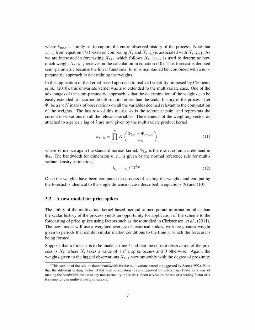
where t0 and t1 denote the start and end of the forecast period, respectively, and Xt, takesthe value 1 if a price spike occurs at time t and 0 otherwise, and ht (or pt) is the forecasthazard/probability for time t. In the results reported here, the value of κ is taken to be 0.5so that the failure to predict an actual spike is penalised at three times the rate of a falsealarm. The resulting loss measure results for input combinations involving change in load(rather than load) and temperature are displayed in Table 5. These loss measures thereforeprovide the opportunity for a more detailed comparison of performance.

NSW Qld SA Vic

ACH MAE 0.0777 0.0777 0.1070 0.1060RMSE 0.1914 0.1931 0.2999 0.2335LPSE 0.1364 0.1318 0.3382 0.1836Asym. 0.0734 0.0799 0.1492 0.1084

X,T1,T2,L2,D1,N1 MAE 0.0339 0.0381 0.0464 0.0500RMSE 0.1392 0.1537 0.1709 0.1816LPSE 0.0800 0.1016 0.1300 0.1385Asym. 0.0359 0.0403 0.0536 0.0563

X,T1,T2,L2,D2,N2 MAE 0.0325 0.0389 0.0460 0.0507RMSE 0.1367 0.1541 0.1669 0.1773LPSE 0.0712 0.1023 0.1080 0.1173Asym. 0.0346 0.0403 0.0522 0.0552

S,T1,T2,L2,D3,N3 MAE 0.0339 0.0387 0.0475 0.0509RMSE 0.1408 0.1557 0.1717 0.1773LPSE 0.0824 0.1034 0.1315 0.1749Asym. 0.0359 0.0408 0.0536 0.0560

Table 5: Errors in forecast probabilities of extreme price events. Upper panelrefers to forecasts made using the ACH model, lower panels refer to the vari-ous semi-parametric model versions. Variable key: Refer to Table 2).

On all symmetric and asymmetric measures (MAE, RMSE, LPSE, Asym) and across all re-gions, the semi-parametric kernel forecasting procedure can be seen to outperform the ACHmodel. On the basis of the LPSE measure, which Rudebusch and Williams (2009) advocateas being the most appropriate for evaluating forecast probabilities, the input combination of(X,T1,T2,L2,D2,N2) yielded the lowest levels for all states except SA which produceda minimum for the input combination of (X,T1,T2,L2,D1,N1), with . On the basis ofthe Asym measure (using a κ of 0.5), the input combination of (X,T1,T2,L2,D2,N2)yielded the lowest levels across all states and thus confirms this combination as giving thebest performance.

16

5.3 A simple trading scheme

A quarterly futures contract is available in the Australian electricity market. The existenceof such therefore provides the basis for further consideration of the forecast performance ofthe proposed semi-parametric method by means of an investigation into the profitability ofan informal trading scheme based on electricity futures contracts. The same trading schemewas used in Christensen, et al., (2011) thus again allowing the results from the ACH model,as well as an unconditional model, to be compared to the semi-parametric method proposedin this paper.

A quarterly futures contract is available in the Australian electricity market which fixes theprice of electricity to the retailer for the life of the contract. The three month out-of-sampleperiod established in this paper for the previous forecast evaluations is therefore suitablealso to allow this trading scheme analysis. At time t during the life of the contract, thehedged price in terms of the futures contract is calculated as the time-weighted average ofthe following components:

1. the mean of the actual spot electricity price for each half hour from the start of thecontract to the current time t, and

2. the mean of the consensus of analysts’ forecasts of price for each half hour for theremainder of the contract (as no futures prices or consensus forecasts are publiclyavailable, synthetic futures contracts are priced by taking the consensus forecast ofprice to be the average price for the same half hour on the same weekday in the samemonth for the previous five years for the relevant region).

The lack of publicly available futures prices, as well as the consensus forecasts, will havean impact on the results of the scheme. It is therefore important to note that, due to suchshortcomings, the results of this exercise should be interrupted more as an illustration ofthe forecast performance of the models rather than evidence of a profitable futures tradingstrategy. Further, for the purposes of this exercise, transaction costs will also be ignored.

The simple trading scheme is therefore as follows. If a time t− 1 the one-step-ahead prob-ability of a price spike at time t exceeds a threshold probability of 0.5 (i.e. if a spike isforecast), the futures contract is entered into. The contract is closed out at time t + k pro-vided the forecast probability of a spike exceeds the threshold in each interval up to timet + k but falls below the threshold at time t + k + 1. The return to this strategy is there-fore the difference between the actual pool price and the hedge price specified in terms ofthe futures contract. Table 6 shows the returns from the unconditional and ACH modelsused as a benchmark from Christensen, et al., (2011), as well as those from several inputcombinations of the proposed semi-parametric kernel method. It should be noted that theunconditional model was generated using 10,000 samples of the length of the forecast pe-riod, drawn from the U[0, 1] distribution such that for each half hour period, the probabilityof a spike was set to a random number from the U[0, 1] and thus if 0.5 or greater then aspike predicted.

17

NSW Qld SA Vic% % % %

Unconditional 14.53 6.21 2.80 5.87ACH 21.47 8.02 0 24.22X,T1,T2,L2,D1,N1 21.17 20.28 22.68 25.54X,T1,T2,L2,D2,N2 21.56 20.68 23.13 26.22X,T1,T2,L2,D3,N3 21.32 20.13 23.60 25.68

Table 6: Trading scheme returns. The first panel shows the 99th percentilereturn for each region using the unconditional model, as well as the returnfor each region based on the ACH model, as presented in Christensen, et al.,(2011). The second panel shows the return for several input combinations tothe proposed new semi-parametric model. Variable key: Refer to Table 2).

The trading scheme exercise provides additional evidence of the usefulness of the proposedsemi-parametric kernel model. Although yielding a similar result to that of the ACH modelfor NSW, the model demonstrated significant improvements on the ACH results for Qld, SAand Vic. In all states except SA, the specific input combination of (X,T1,T2,L2,D2,N2)produced the highest return and is therefore consistent with previously used forecast eval-uation measures. The relatively small increase to return for NSW may be the result ofincreased correct predictions cancelling with increased false alarms, or possibly the effectof inaccurate forecasting at the beginning and end of spike series. Where as for Qld, SA andVic the proposed semi-parametric method was clearly more successful, possibly as a resultof the methods ability to produce a much higher proportion of correct predictions comparedto the ACH model. The trading scheme exercise therefore shows further the ability of theproposed semi-parametric method to yield more successful and consistent forecasting thanprevious methods.

6 Probability threshold modification

The success of the proposed semi-parametric kernel method to forecast spikes in electricityprices has been shown only to be limited with regard to its ability to specifically predict thebeginning and end of a spike series, such an aspect being particularly difficult regardless ofthe time series application. Investigation of possible modifications to improve this aspectis therefore warranted, given the overall success already demonstrated. The obvious choicefor an extension being to use a dynamic scheme in which the probability threshold is variedso as to possibly increase the instance of first spike identification. Several choices existwhich will be explored briefly in this section to determine whether such improvement canbe achieved.

A simple scheme of varying the fixed threshold probability of 0.5 to other levels can be

18

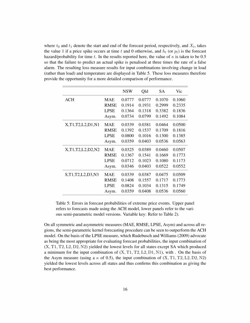
considered initially to gauge the effect of this parameter. Focusing on NSW, a preliminaryunderstanding of the link can be developed, as shown in Table 7.

Threshold Correct False First Last0.1 264 91 17 00.15 255 60 8 00.2 253 54 6 00.25 251 51 4 10.3 247 48 2 10.35 244 46 1 20.4 240 46 1 20.45 236 44 1 30.5 235 42 1 5

Table 7: Impact of a reduced probability threshold in predicting a spikeusing the proposed semi-parametric method with an input combination of(X,T1,T2,L2,D2,N2). Variable key: Refer to Table 2).

These results clearly show that a lower probability threshold will increase the number ofcorrect spike forecasts, however this increase occurs simultaneously with an increase inthe number of false alarms. Interestingly, a lower threshold also increases the numberof correctly forecast first spikes. This can be contrast to the lower threshold reducing thenumber of last spikes in a series to be correctly forecast. These results therefore indicate thata lower threshold is useful only in the context of forecasting the beginning of a new spikeseries and therefore the possibility of a dual threshold strategy in which a lower thresholdis useful to detect the beginning of a spike series, after which a higher threshold is used todetermine forecasts for the continuance of the series. The results of a scheme in which athreshold of 0.1 is used to forecast the first spike and a threshold of 0.75 used for subsequentspikes is shown in Table 8 for all regions.

NSW Qld SA VicCorrect 217 170 291 302False 62 69 54 104First 17 7 7 16Last 12 8 5 11

Table 8: Impact of a dual probability threshold scheme in predicting a spikeusing the proposed semi-parametric method with an input combination of(X,T1,T2,L2,D2,N2). Specifically a threshold of 0.1 is used to forecastthe first spike and a threshold of 0.75 used for subsequent spikes. Variablekey: Refer to Table 2).

On the basis of these simple benchmark figures, the dual probability threshold scheme isclearly superior to that of a single threshold of 0.5 (refer also to Table 3 and Table 4). Table

19

8 shows that this modified scheme is able to correctly forecast 32.7%, 11.4%, 11.3% and20.8% of the first spikes for NSW, Qld, SA and Vic respectively. Also, that it is able tocorrectly forecast 23.1%, 13.1%, 8.1% and 14.3% of the end spikes for NSW, Qld, SA andVic respectively. Overall it can therefore be seen that this extension to the proposed semi-parametric kernel method was able to provide valuable insight into understanding the pricespiking process, as well as improved results7.

7 Conclusion

Electricity markets are often structured so as to allow retailers to purchase at an unregu-lated spot price but then sell to consumers at a heavily regulated price. The occurrence ofextreme movements of the spot price of electricity represent a significant source of risk toretailers. As such, the ability to forecast price spikes is an important aspect of effectiverisk management. The contribution of this paper was to propose a semi-parametric fore-casting scheme to forecast price spikes in which the weights assigned to historical eventsare state-dependent rather than time-dependent and are determined, roughly speaking, byhow similar each occurrence in the sample is to a current point of reference by the ap-plication of a multivariate kernel function. It was found that the semi-parametric methodproduces forecasts that are more accurate than the previously identified best approach. Thissuperior performance is attributable to the semi-parametric approach capturing the inherentnonlinearity in the spike process.

7Other schemes were also considered, including progressive modification to the probability threshold duringthe occurrence of a series so as to cause the probability threshold to increase linearly, as well as exponentially.However, neither such strategy was able to achieve results comparable to that of the dual threshold scheme.

20

References

Anderson, E. J., Hu, X. and Winchester, D. (2006). Forward contracts in electricity mar-kets: The Australian experience. Energy Policy, 35, 3089–3103.

Barlow, M. T. (2002). A diffusion model for electricity prices. Mathematical Finance, 12,287–298.

Becker, R., Hurn, A. S. and Pavlov, V. (2007). Modelling spikes in electricity prices.Economic Record, 83, 371–382.

Cartea, A. and Figueroa, M. G. (2005). Pricing in electricity markets: A mean revertingjump diffusion model with seasonality. Applied Mathematical Finance, 12, 313–335.

Christensen, T.M., Hurn, A.S., and Lindsay, K.A. (2011). Forecasting Spikes in ElectricityPrices. NCER Working Paper Series 70, National Centre for Econometric Research.

Becker, R., Clements, A.E., and Hurn, A.S. (2010). Semi-parametric forecasting of real-ized volatility. Studies in Nonlinear Dynamics & Econometrics, vol. 15(3), pages 1.

Cleveland, W.S. (1979). Robust locally weighted regression and smoothing scatterplots.Journal of the American Statistical Society, 74, 829-836.

de Jong, C. and Huisman, R. (2003). Option pricing for power prices with spikes. EnergyPower Risk Management, 7, 12–16.

Engle, R. F. and Russell, J. R. (1998). Autoregressive Conditional Duration: A New Modelfor Irregularly Spaced Transaction Data. Econometrica, 66(5), 1127–1162.

Escribano, A, Pena, J. I. and Villaplana, P. (2002). Modelling electricity prices: Interna-tional evidence. Working Paper 02-27, Universidad Carlos III de Madrid.

Fernandes, M. and Grammig, J. (2006). A family of autoregressive conditional durationmodels. Journal of Econometrics, 130(1), 1–23.

Geman, H. and Roncorni, A. (2006). Understanding the fine structure of electricity prices.Journal of Business, 79, 1225–1261.

Hambly, B., Howson, S. and Kluge, T. (2007). Modelling Spikes and Pricing Options inElectricity Markets. Working Paper. University of Oxford.

Hamilton, J. D. and Jorda, O. (2002). A Model of the Federal Funds Rate Target. Journalof Political Economy, 110(5), 1135–1167.

Kanamura, T. and Ohashi, K. (2007). On transition probabilities of regime switching inelectricity prices. Energy Economics, 30, 1158–1172.

21

Knittel, C. R. and Roberts, M. R. (2005). An empirical examination of restructured elec-tricity prices. Energy Economics, 27, 791–817.

Mizrach, B. (1992). Multivariate nearest-neighbour forecasts of EMS exchnage rates.Journal of Applied Econometrics, 7, S151-S163.

Mount, T. D., Ning, Y. and Cai, X. (2006). Predicting price spikes in electricity marketsusing a regime-switching model with time-varying parameters. Energy Economics, 28,62–80.

Rudebusch, G. D. and Williams, J. C. (2009). Forecasting Recessions: the puzzle of theenduring power of the yield curve. Journal of Business and Economic Statistics, vol. 27(4),pages 492-503.

Scott, D.W. (1992). Multivariate Density Estimation: Theory, Practice and Visualization,New York: John Wiley.

Silverman, B.W. (1986). Estimation for Statistics and Data Analysis, London: Chapmanand Hall.

Weron, R., Bierbrauer, M. and Truck, S. (2004). Modelling electricity prices: jump diffu-sion and regime switching. Physica A, 336, 39–48.

22

Semi-parametric forecasting of Spikes in Electricity … forecasting of Spikes in Electricity Prices...

Documents

Transcript of Semi-parametric forecasting of Spikes in Electricity … forecasting of Spikes in Electricity Prices...