Electricity Demand Forecasting Methodology Information Paper
80
Electricity Demand Forecasting Methodology Information Paper August 2020
Transcript of Electricity Demand Forecasting Methodology Information Paper

Electricity Demand Forecasting Methodology Information Paper
August 2020

Important notice
PURPOSE
AEMO has prepared this document to provide information about methodologies used to forecast annual
consumption and maximum and minimum demand in the National Electricity Market (NEM) for use in
planning publications such as the Electricity Statement of Opportunities (ESOO), and the Integrated System
Plan (ISP).
The methodologies described here may also be considered in other jurisdictions, such as forecasting demand
in the Wholesale Electricity Market (WEM) in Western Australia.
DISCLAIMER
This report contains input from third parties, and conclusions, opinions or assumptions that are based on
that input.
AEMO has made every effort to ensure the quality of the information in this document but cannot guarantee
that information and assumptions are accurate, complete or appropriate for your circumstances.
Anyone proposing to use the information in this document should independently verify and check its
accuracy, completeness and suitability for purpose, and obtain independent and specific advice from
appropriate experts.
Accordingly, to the maximum extent permitted by law, AEMO and its officers, employees and consultants
involved in the preparation of this document:
• make no representation or warranty, express or implied, as to the currency, accuracy, reliability or
completeness of the information in this document; and
• are not liable (whether by reason of negligence or otherwise) for any statements or representations in
this document, or any omissions from it, or for any use or reliance on the information in it.
VERSION CONTROL
Version Release date Changes
1 27/8/2020 Initial release of the 2020 demand forecasting methodologies
© 2020 Australian Energy Market Operator Limited. The material in this publication may be used in
accordance with the copyright permissions on AEMO’s website.

© AEMO 2019 | Electricity Demand Forecasting Methodology Information Paper 3
Contents 1. Introduction 6
1.1 Forecasting principles 6
1.2 Modelling consumer behaviour 6
1.3 Key definitions 8
1.4 Changes since the previous version of this methodology 10
2. Business annual consumption 12
2.1 Data sources 12
2.2 Methodology 13
3. Residential annual consumption 21
3.1 Data sources 21
3.2 Methodology 22
4. Operational consumption 30
4.1 Small non-scheduled generation 30
4.2 Network losses and auxiliary loads 32
5. Maximum and minimum demand 34
5.1 Data preparation 35
5.2 Exploratory data analysis 35
5.3 Model development and selection 36
5.4 Simulate base year (weather and calendar normalisation) 39
5.5 Forecast probability of exceedance for base year 40
5.6 Forecast probability of exceedance for long term 40
6. Half-hourly demand traces 43
6.1 Growth (scaling) algorithm 45
6.2 Pass 1 – growing to OPSO-lite targets 45
6.3 Pass 2 – reconciling to the OPSO targets 46
6.4 Pass 3 – adding coordinated EV charging to OPSO 46
6.5 Reporting 46
A1. Electricity retail pricing 47
A2. Weather and climate 49
A2.1 Heating Degree Days (HDD) and Cooling Degree Days (CDD) 49
A2.2 Determining HDD and CDD standards 50
A2.3 Climate change 50
A3. Rooftop PV and energy storage 53
A3.1 Rooftop PV forecast 53

© AEMO 2019 | Electricity Demand Forecasting Methodology Information Paper 4
A3.2 Energy storage systems forecast 55
A4. Electric vehicles 58
A5. Connections and uptake of electric appliances 60
A5.1 Connections 60
A5.2 Uptake and use of electric appliances 61
A6. Data sources 65
A7. Data segmentation 68
A7.1 AER-derived annual residential-business split: top-down method 68
A7.2 Residential delivered daily residential-business split: bottom-up method 71
A8. Demand trace scaling algorithm 75
Abbreviations 79
Tables Table 1 Historical and forecast input data sources for business sector modelling 12
Table 2 Short-term base model variable description 17
Table 3 SME model variable description 18
Table 4 Historical input data sources for residential sector modelling 21
Table 5 Forecast input data sources for residential sector modelling 21
Table 6 Weather normalisation model variable description 25
Table 7 Variables and descriptions for residential consumption model 27
Table 8 Residential base load, heating load and cooling load model variables and descriptions 28
Table 9 List of variables included for half-hourly demand model 37
Table 10 List of variables included for half-hourly demand model 38
Table 11 Residential pricing model component summary 48
Table 12 Critical regional temperatures for HDD and CDD 49
Table 13 Weather stations used for HDD and CDD 50
Table 14 Mapping of consultant trajectories used for DER forecasts 53
Table 15 New South Wales Central scenario tariff and associated battery operating type shares 56
Table 16 Assumed proportion of daytime charging that is managed, by scenario 59
Table 17 Assumed proportion of night-time charging that is managed, by scenario 59
Table 18 List of appliance categories used in calculating the appliance growth index 62
Table 19 COVID adjustments to the appliance growth indices 64
Table 20 ANZSIC code mapping for industrial sector disaggregation 65

© AEMO 2019 | Electricity Demand Forecasting Methodology Information Paper 5
Table 21 Historical and forecast input data sources 66
Table 22 Prepared demand trace and targets 76
Table 23 Scaling ratios 76
Table 24 Resulting energy 77
Table 25 Check of grown trace against targets 77
Figures Figure 1 Example individual and group demand shown on one day 7
Figure 2 Scatterplot of New South Wales demand and temperature, example based on 2017
calendar year 7
Figure 3 Operational demand/consumption definition 10
Figure 4 Steps for large industrial load survey process 13
Figure 5 Aggregation process for final delivered forecast 20
Figure 6 Process flow for residential consumption forecasts 23
Figure 7 Aggregation process for final residential underlying forecast 28
Figure 8 Aggregation process for final residential delivered forecast 29
Figure 9 Demand relationships 30
Figure 10 Conceptual summer maximum demand probability density functions for three scenarios 34
Figure 11 Theoretical distribution of annual half-hourly data to derive maxima distribution 41
Figure 12 Demand trace development process flow diagram 44
Figure 13 Example of north-facing vs west-facing PV generation 55
Figure 14 New South Wales average daily February profile 57
Figure 15 Energy services vs energy consumption 61
Figure 16 Hybrid model used to calculate the half-hourly residential and business split 68
Figure 17 Workflow of the bottom-up method for residential-business split 72
Figure 18 Prepared demand trace 75
Figure 19 Day-type categories 76
Figure 20 Grown trace and targets 77

© AEMO 2019 | Electricity Demand Forecasting Methodology Information Paper 6
1. Introduction
AEMO produces independent customer electricity demand forecasts for use in publications such as the
Electricity Statement of Opportunities (ESOO) and the Integrated System Plan (ISP). These forecasts provide
projections of customer connections, customer technology adoption, electricity consumption, maximum and
minimum demand over a forecast period up to 30 years for each region of the National Electricity Market
(NEM) and up to 10 years for the Wholesale Electricity Market (WEM). This report outlines the forecasting
methodologies in use.
1.1 Forecasting principles
AEMO is committed to producing quality forecasts that support informed decision-making. For decision-
makers to act on forecasts, they must be credible and dependable. Forecasting principles help guide the
multitude of decisions that need to be made towards this goal. Principles guide choices about how the
forecasts are done, particularly where there are trade-offs in outcome. For example, simplicity versus
comprehensiveness, speed versus insight.
To achieve this, AEMO’s forecast team work to three main objectives:
1. Transparency – to ensure inputs and forecast methodologies are well understood.
– AEMO consults broadly to develop scenario inputs and model methodologies. This document further
aims to improve adequate stakeholder understanding of the methodologies deployed.
2. Accountability – to measure forecasting performance, refine and improve where issues are
detected.
– AEMO monitors the accuracy of past forecasts by comparing actual data against forecasted data.
Forecasting accuracy reports1 explore both the levels of accuracy and any causes of inaccuracy and
have generated numerous process improvements.
3. Accuracy – to adopt best practise methodologies and monitor lead indicators of change.
– AEMO employs good practises, such as developing clear work instructions, clearly identifying
information sources and using best practise model development techniques.
1.2 Modelling consumer behaviour
Individual consumers do not behave consistently every day and can sometimes behave unpredictably. Even
on days with identical weather, the choices of individuals are not identical, and reflect the lifestyle of the
household, or operation of the business. It is only when customer electrical demand is aggregated to a
regional level that the group behaviour becomes more predictable. This is because the group demand largely
cancels out the idiosyncratic behaviour of the individual.
1 Forecasting accuracy reports can be found at https://www.aemo.com.au/Electricity/National-Electricity-Market-NEM/Planning-and-forecasting/Forecasting-
Accuracy-Reporting

© AEMO 2019 | Electricity Demand Forecasting Methodology Information Paper 7
Figure 1 shows the load profile of an individual customer, compared to the average of a group of similar
customers. While the load profile of the individual is spikey and erratic, the group profile has smoothed out
some of idiosyncrasies of the customer.
Figure 1 Example individual and group demand shown on one day
Although demand becomes more predictable when aggregated, it remains a function of individual customer
decisions. Periods of high demand only become so because individual customers choose to do the same
things at the same time. Peak demand is therefore driven by the degree of coincident appliance use across
customers, across regions. There are many factors that drive customers to make similar appliance choices at
the same time including:
• Work and school schedules, traffic and social norms around meal times.
• Weekdays, public holidays, and weekends.
• Weather, and the use of heating and cooling appliances.
• Many other societal factors, such as whether the beach is pleasant, or the occurrence of retail promotions.
Figure 2 shows a scatter plot of temperature and electrical load. A strong relationship between temperature
and group electrical load can be seen, however the relationship cannot explain all variations. Even when all
observable characteristics are considered, the variance attributable to coincident customer choices remains.
Figure 2 Scatterplot of New South Wales demand and temperature, example based on 2017 calendar
year

© AEMO 2019 | Electricity Demand Forecasting Methodology Information Paper 8
It is standard industry practise to model the drivers of demand in two parts:
• Structural drivers, which are modelled as scenarios, including considerations such as:
– Population.
– Economic growth.
– Electricity price.
– Technology adoption.
– Atmospheric greenhouse gas concentration.
• Random drivers, which are modelled as a probability distribution, including considerations such as:
– Weather-driven coincident customer behaviour.
– Weather-driven embedded generation output.
– Non-weather-driven coincident customer behaviour.
The methods deployed by AEMO are consistent with standard industry practice, in that:
• numerous scenarios are developed to test uncertainty in structural drivers.
• maximum and minimum demand forecasts use probability distributions to describe uncertainty in random
drivers.
Consumption and demand forecasts are based on aggregated customer segments:
• Residential: residential customers only.
• Business: includes industrial and commercial users. This sector is categorised into large industries and
small/medium sized businesses (subcategorised further in accordance with Section 2) as follows:
– Large industrial loads (LIL), including transmission-connected facilities, and
– Small/medium businesses, covering any distribution connected loads not included in the LIL category.
1.3 Key definitions
AEMO forecasts are reported as2:
• Operational: Electricity demand is measured by metering supply to the network rather than what is
consumed. Operational refers to the electricity used by residential, commercial and large industrial
consumers, as supplied by scheduled, semi-scheduled, and significant non-scheduled generating units
with aggregate capacity ≥ 30 megawatts (MW). Operational demand generally excludes electricity
demand met by non-scheduled wind/solar generation of aggregate capacity < 30 MW, non-scheduled
non-wind/non-solar generation and exempt generation.
The exceptions which are included in the operational demand definition are:
– Yarwun (registered as non-scheduled generation but treated as scheduled generation).
– Mortons Lane wind farm, Yaloak South wind farm, Hughenden solar farm, Longreach solar farm (non-
scheduled generation < 30 MW but due to power system security reasons AEMO is required to model
in network constraints).
– Non-scheduled diesel generation in South Australia.
2 More definition information is at https://www.aemo.com.au/-
/media/files/electricity/nem/security_and_reliability/dispatch/policy_and_process/2020/demand-terms-in-emms-data-model.pdf.

© AEMO 2019 | Electricity Demand Forecasting Methodology Information Paper 9
– Batteries that are owned, operated or controlled with a nameplate rating of 5 MW or above, as these
need to be registered as both a scheduled generator and a market customer.3
– Intermittent Loads in Western Australia4.
• Consumption: Consumption refers to electricity used over a period of time, conventionally reported as
gigawatt hours (GWh). It is reported on a “sent-out” basis unless otherwise stated (see below for
definition).
• Demand: Demand is defined as the amount of power consumed at any time. Maximum and minimum
demand is measured in MW and averaged over a 30-minute period. It is reported on a “sent-out” basis
unless otherwise stated (see below for definition).
• “As generated” or “sent out” basis: “Sent out” refers to electricity supplied to the grid by scheduled,
semi-scheduled, and significant non-scheduled generators (excluding their auxiliary loads, or electricity
used by a generator). “As generated” refers to the same consumption, but including auxiliary loads, or
electricity used by a generator.
• Auxiliary loads: Auxiliary load, also called ‘parasitic load’ or ‘self-load’, refers to energy generated for use
within power stations, but excludes pumped hydro. The electricity consumed by battery storage facilities
within a generating system is not considered to be auxiliary load. Electricity consumed to charge by
battery storage facilities is a primary input and treated as a market load.
Other key definitions used are:
• Probability of Exceedance (POE): POE is the likelihood a maximum or minimum demand forecast will be
met or exceeded. A 10% POE maximum demand forecast, for example, is expected to be exceeded, on
average, one year in 10, while a 90% POE maximum demand forecast is expected to be exceeded nine
years in 10.
• Rooftop PV: Rooftop PV is defined as a system comprising one or more photovoltaic (PV) panels, installed
on a residential or commercial building rooftop to convert sunlight into electricity. The capacity of these
systems is less than 100 kilowatts (kW).
• PV Non-Scheduled Generators (PVNSG): PVNSG is defined as PV systems larger than 100 kW but smaller
than 30 MW non-scheduled generators.
• Other Non-Scheduled Generators (ONSG): ONSG represent non-scheduled generators that are smaller
than 30 MW and are not PV.
• Energy Storage Systems (ESS): ESS are defined as small distributed battery storage for residential and
commercial consumers.
• Electric Vehicle (EV): EVs are residential and business battery powered vehicles, ranging from small
residential vehicles such as motor bikes or cars to large commercial trucks
Figure 3 provides a schematic of the breakdown and linkages between demand definitions. Operational
demand “sent out” is computed as the sum of residential, commercial and large industrial customer electricity
consumption plus distribution and transmission losses minus rooftop PV, PVNSG and ONSG.
3 Registering a Battery System in the NEM – Fact Sheet is at https://aemo.com.au/-/media/Files/Electricity/NEM/Participant_Information/New-
Participants/battery_fact_sheet_final.pdf.
4 Intermittent Loads are electricity loads that have behind the fence generation that are also connected to the grid. On occasion, these loads draw electricity
from the grid.

© AEMO 2019 | Electricity Demand Forecasting Methodology Information Paper 10
Figure 3 Operational demand/consumption definition
* Including VPP from aggregated behind-the-meter battery storage.
** For definition, see: https://www.aemo.com.au/-/media/files/electricity/nem/security_and_reliability/dispatch/policy_and_process/2020/
demand-terms-in-emms-data-model.pdf.
1.4 Changes since the previous version of this methodology
This is the 2020 version of AEMO’s Electricity Demand Forecasting Methodology Information Paper. It was last
refreshed with the 2019 ESOO, in August 2019.
Since that publication, AEMO has updated its forecasts in accordance with data updates, as outlined in the
companion Inputs, assumptions and scenarios report (IASR)5. In addition to data updates, AEMO has updated
the methodologies applied to forecast electricity consumption, maximum and minimum demand as follows:
Continuous improvements to existing methodologies:
• Business annual electricity consumption forecast: As outlined in the Forecast Accuracy Report, AEMO
improved its business consumption forecast model by forecasting the small-medium enterprise (SME)
sector with reference to a near-term trend in consumption, before extending to a longer term forecast
approach. The addition of the near-term trend method was outlined as a key improvement to ensure that
the short term dynamics and a transition to the scenario conditions affecting energy consumption were
reflected in the forecast, before economic and technical fundamentals produce the longer term trajectory.
• Large industrial loads associated with water infrastructure facilities: This sector has been improved in
the 2020 forecast by identifying and including additional existing desalination facilities that were not
explicitly included within the 2019 forecast.
• Distributed PV uptake forecasts: As outlined in the 2019 Forecast Accuracy Report6, distributed PV
installations have exceeded previous estimates as customer investment in DER has outpaced recent
expectations. AEMO and its DER consultants – CSIRO and Green Energy Markets in 2020 – explicitly
sought to improve the PV forecasts. For CSIRO, this included greater consideration of the near-term trend
as an explicit short term model (conceptually similar to the SME forecast trend model described above).
GEM’s forecasts also consider installer surveyed market intelligence. In working with the DER consultants,
5 AEMO, 2020 Inputs, Assumptions and Scenarios Report, at https://www.aemo.com.au/Electricity/National-Electricity-Market-NEM/Planning-and-
forecasting/Inputs-Assumptions-and-Methodologies.
6 At https://aemo.com.au/en/energy-systems/electricity/national-electricity-market-nem/nem-forecasting-and-planning/forecasting-and-reliability/
forecasting-accuracy-reporting
Scheduled Loads
Network Losses
Auxiliaries
Residential Customers
Business Customers
‘Operational’ Consumption/demand
‘Operational’ is met by these generators
Excluded from ‘Operational’
Auxiliaries
Transmission and Distribution Network
Auxiliaries
Photo voltaic Non-Scheduled Generation (PVNSG)
Scheduled* & Semi-Scheduled Generation
Significant Non-Scheduled Generation **
Operational ‘As Generated’
Operational ‘Sent Out’
Auxiliaries
Other Non-Scheduled Generation (ONSG)
Underlying demand
Delivered demand
Rooftop PV and non-VPP battery storage(netted of underlying demand to give delivered demand)

© AEMO 2019 | Electricity Demand Forecasting Methodology Information Paper 11
AEMO also received the latest information available at the time from the Clean Energy Regulator (CER) to
assist in model calibration.
• Updated appliance index and dwelling forecast: AEMO has developed an improved, updated
residential and appliance stock model to ensure appropriate consideration of building age, size and
building material quality informs the forecasts of energy efficiency and connections forecasts.
• Maximum/minimum demand annual growth: Forecast maximum/minimum demand has been changed
is grown year-on-year by a composite growth index based on drivers like population, economic growth
and price, rather than indices specific to baseload, heating and cooling used previously. This was found to
get better alignment with the historical change in relationship between annual maximum demand and
consumption figures.
• ONSG and maximum/minimum demand: Generation from peaking-type ONSG units is now modelled as
DSP7 rather than being an offset to maximum/minimum demand.
• Coordinated EV charging: Additional step added to half-hourly trace growing algorithm, that each day
spreads coordinated EV charging across the lowest demand periods.
• Inclusion of specific Covid-19 effects in most forecasting components: The methodology has been
adjusted to accommodate the impact of the COVID-19 pandemic, which is introducing social, economic
and operational challenges to many sectors, including energy. Specifically:
– The methodology for adjusting the consumption forecast for structural shocks (such as COVID-19) is
described in this report.
– The high-level approach for adjusting the maximum/minimum demand forecasts for structural shocks
(such as COVID-19) is described in this report (with the details as an appendix to the ESOO itself).
– The COVID-19 impacts on key economic inputs is described in the IASR.
7 See https://aemo.com.au/-/media/files/stakeholder_consultation/consultations/nem-consultations/2020/demand-side-participation/final/demand-side-
participation-forecast-methodology.pdf.

© AEMO 2019 | Electricity Demand Forecasting Methodology Information Paper 12
2. Business annual consumption
The business sector captures all non-residential consumers of electricity in the NEM and the WEM. These
have been segmented into two broad categories, recognising the different drivers affecting forecasts. This
sector is further categorised into large industries and small to medium sized businesses, to apply an
integrated, sectoral-based approach to business forecasts to capture structural changes in the Australian
economy:
• Large industrial loads (LIL) – further split into subcategories:
– Aluminium smelting – including Bell Bay, Boyne Island, Portland, and Tomago aluminium smelters.
Note: This does not apply to the WEM.
– Coal mining – customers mainly engaged in open-cut or underground mining of bituminous thermal
and metallurgical coal. Note: This does not apply to the WEM.
– Coal seam gas (CSG) – associated with the extraction and processing of CSG for export as liquefied
natural gas (LNG) or supplied to the domestic market. Note: This does not apply to the WEM.
– Mining and minerals processing facilities – customers mainly engaged in open-cut or underground
mining of non-coal and aluminium minerals and the pre-processing of these minerals. Note: This only
applies to the WEM.
– Water infrastructure facilities –all large water treatment facilities, including desalination, for potable
water, wastewater treatment and water pumping.
– Other transmission- and distribution-connected customers – covering any transmission- and
distribution-connected loads not accounted for in the categories above.
• Small to medium enterprises (SME) – any distribution-connected loads not included in the LIL category.
• Electric vehicles (EV) – covering commercial fleet, trucks and buses.
2.1 Data sources
Business sector modelling relies on a combination of sources for input data where possible. Table 1 outlines
the schedule of sources for each data series for both the NEM and the WEM.
Table 1 Historical and forecast input data sources for business sector modelling
Data series Source 1 Source 2 Source 3
Electricity consumption
data AEMO Database Transmission and distribution
industrial surveys
Historical consumption data
by industry sector Dept. of Energy and
Environment (Table F)
Economic data* ABS External Economic Consultancy
© AEMO 2019 | Electricity Demand Forecasting Methodology Information Paper 13
Data series Source 1 Source 2 Source 3
Retail electricity price Retail Standing Offers AEMC Price Trend Report 2019 ISP
Wholesale electricity price AEMO
Energy efficiency AEMO based on 2019
consultancy
State government departments
for some regions
Rooftop PV/battery/electric
vehicle generation External Consultancy
* Economic data includes Gross State Product and Household Disposable Income.
2.2 Methodology
The overall approach to forecasting business consumption for both markets is to measure the
energy-intensive large loads separately from broader business sector, based on the observation that each
load historically is subject to different underlying drivers. AEMO periodically reviews whether further
segmentation of the business sector is feasible; the availability of consumption data and the size of sector are
limiting factors to whether AEMO can monitor the segments separately.
Either surveys or standard econometric methods were used to forecast consumption in these sectors:
• Large industrial loads (LIL): survey-based forecasts.
• Small to medium enterprises (SME): econometric modelling.
2.2.1 Large Industrial Load forecast
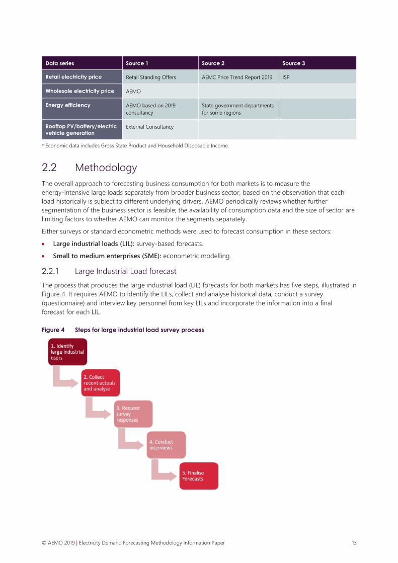
The process that produces the large industrial load (LIL) forecasts for both markets has five steps, illustrated in
Figure 4. It requires AEMO to identify the LILs, collect and analyse historical data, conduct a survey
(questionnaire) and interview key personnel from key LILs and incorporate the information into a final
forecast for each LIL.
Figure 4 Steps for large industrial load survey process

© AEMO 2019 | Electricity Demand Forecasting Methodology Information Paper 14
Identify large industrial users
AEMO maintains a list of LILs identified primarily by interrogating AEMO’s meter data and working with
transmission network operators and distribution network operators for each region. A threshold of demand
greater than 10 MW for greater than 10% of the latest financial year is used to identify those loads. This
threshold aims to capture the most energy intensive consumers in each region.
The list is further validated and updated using two methods:
• Distribution and transmission surveys: requesting information on aggregate and new loads.
• Media search: augmenting the existing portfolio of LILs with new industrial loads if AEMO is made aware
of such users through joint planning with network service providers, public sources including media,
conferences and industry forums.
Collect historical data (recent actuals) and analyse
Updates to historical consumption data for each LIL were analysed to:
• Understand consumption trends at each site and develop targeted questions (if required).
• Prioritise industrial users to improve the effectiveness of the interview process.
Request survey responses and conduct interviews
Step 1: Initial survey
AEMO surveys identified LILs8 requesting historical and forecast electricity consumption information by site.
The survey requested annual electricity consumption and maximum demand forecasts for three scenarios in
the NEM and the WEM, where the economy follows:
1. The most likely economic pathway.
2. A stronger economic pathway.
3. A weaker economic pathway.
Step 2: Detailed interviews
After the survey is issued, only prioritised large industrial users are contacted directly to expand on their
survey responses. This includes discussions about:
• Key electricity consumption drivers, such as exchange rates, commodity pricing, availability of feedstock,
current and potential plant capacity, mine life, and cogeneration.
• Current exposure of business to spot pricing and management of price exposures, such as contracting
with retailers, Power Purchase Agreements and hedging.
• Future management of prices and impact of prices on consumption, based on AEMO provided guidelines.
• Potential drivers of major change in electricity consumption (such as expansion, closure, outages,
cogeneration, fuel substitution).
• Their participation (if any) in Demand Side Management programs.
• Assumptions governing the scenarios.
Not all LILs were interviewed. Interviews with LILs were prioritised based on the following criteria:
• Volume of load (highest to lowest) – movement in the largest volume consumers can have broader
market ramifications (such as an impact on realised market prices).
• Year-on-year percentage variation – assess volatility in load, noting that those with higher usage variability
influences forecast accuracy.
8 Defined by AEMO as those who had a maximum demand of 10 MW or more for at least 10% of the time in a year for each region.
© AEMO 2019 | Electricity Demand Forecasting Methodology Information Paper 15
• Year-on-year absolute variation – relative weighting of industrial load is needed to assess materiality of
individual variations.
• Forecast vs actual consumption and load for historic survey responses – forecast accuracy is an evolving
process of improvement and comparisons between previous year actual consumption and load against
the forecast will help improve model development.
Finalise forecasts
The following subsections detail the methodology for producing forecasts for each subsector for each region.
Aluminium smelting (this does not apply to the WEM)
The aluminium smelting forecast was based on a survey and interview process (see Section 2.2.5). To maintain
confidentiality9, AEMO aggregates forecasts with the econometric results before publishing the LIL forecast.
Coal mining (this does not apply to the WEM)
Coal mining and port service companies are surveyed, and selected operations were interviewed, to obtain a
baseline for the coal industry. The consumption forecast was based on these survey result10.
Coal seam gas (this does not apply to the WEM)
Electricity forecasts for the CSG sector reflect the grid-supplied electricity consumed predominantly in the
extraction and processing of CSG to service sales to domestic consumers or exports of LNG.
AEMO surveyed the CSG consortium following the 2019 GSOO and assessed long-term global trends to
update the CSG forecasts used in the 2020 GSOO. Gas to electricity conversion ratios were calculated using
historical gas and electricity consumption data at the project sites and applied to the 2020 GSOO forecast to
derive the CSG forecasts used in the 2020 ESOO.
Mining and minerals processing facilities (for the WEM only)
All large mining and minerals processing loads in the WEM are surveyed with selected companies interviewed
by site to obtain a baseline for each facility.
Water infrastructure facilities
All large water infrastructure facilities, including desalination, for potable water, wastewater treatment and
water pumping in the NEM and the WEM are surveyed with selected companies interviewed by site to obtain
further information about future water requirements for each facility.
Other transmission- and distribution-connected customers
Other large users of energy that do not fall into the above categories (such as large manufacturers or large
rail networks) are surveyed separately with forecasts based of these results.
2.2.2 Small to medium enterprises (SME) consumption forecast
SME consumption, with LILs removed, contains aggregate consumption data for the non-residential sector
that covers a broad range of activities to which no direct information on usage behaviour is available. As
such, a more detailed forecasting method is applied that accommodates time-series methods capturing the
more predictable patterns in recent usage (such as seasonality, cycles and trend along with causal factors that
encapsulate the long-term structural changes11 that are explored through different scenarios for the sector.
Broadly, the forecast for SME consumption can be written as:
9 As required by the National Electricity Law (NEL).
10 This approach accounts for additional growth in existing assets as well as for new projects.
11 Chase, C, 2009, Demand-Driven Forecasting: A Structured Approach to Forecasting. John Wiley & Sons, Inc., Hoboken, New Jersey.

© AEMO 2019 | Electricity Demand Forecasting Methodology Information Paper 16
𝐹𝑜𝑟𝑒𝑐𝑎𝑠𝑡 = 𝑓(𝑠𝑒𝑎𝑠𝑜𝑛𝑎𝑖𝑙𝑡𝑦, 𝑡𝑟𝑒𝑛𝑑, 𝑐𝑦𝑐𝑙𝑖𝑐𝑎𝑙, 𝑐𝑎𝑢𝑠𝑎𝑙 𝑓𝑎𝑐𝑡𝑜𝑟(𝑠), 𝑢𝑛𝑒𝑥𝑝𝑙𝑎𝑖𝑛𝑒𝑑 𝑣𝑎𝑟𝑖𝑎𝑛𝑐𝑒)
The seasonality is captured through the production of a short-term daily regression model trained on 24
months of data, capturing the effects of weather. A trend and cyclical component analysis is then performed
against longer term data (4-6 years). Unexplained variance is captured by examining year-on-year variance,
once known structural effects are accounted for and the time series is de-trended.
The causal factors are separately analysed against the Department of Energy (Table F)12 long-term data series
(10+years) with large industrial loads removed to smooth out any disjoins before correlating with economic
datasets (causal factors). The data is then scaled to the AEMO SME meter data before incorporation into the
forecast, with other long-term structural drivers such as energy efficiency and price.
These short-term and long-term models are then combined to produce the long-term SME model.
This shift in methodology to include a short-term trend model as well as a longer-term approach was
identified as one of two key improvements from the 2019 Forecast Accuracy Report13.
Short-term time-series model
Time-series models have been described as more applicable in short-term forecasting14 and can be applied
systematically. The short-term SME forecast uses generic time-series methods to model the trend, seasonality,
cyclical and unexplained variance to form a short-term forecast (0-3 years ahead).
The short-term time-series model consists of three stages:
• Calculating a weather-normalised base year (most recent 24 months of consumption data used) capturing
seasonality.
• Determining a trend or cyclical components (4-6 years of consumption data used).
• Estimating uncertainty applicable to the different scenarios.
Base year
The business sector short-term forecast was developed using a linear regression model, using approximately
24 months of consumption with ordinary least squares to estimate coefficients. The independent variables are
described in Table 2 with subscript i representing days for the NEM, and months for the WEM.15
The business forecasts for underlying annual consumption were aggregated by end-use components
(base load, heating, and cooling components).
The first stage of the short-term forecast, is to produce the Base Year, that applies a median weather year
(weather normalised) . This gives a starting point (to reflect current consumption patterns) that considers
intra-year variation to seasonality, holidays and weather. Structural effects that affect the data series are also
able to be captured, such as COVID-19. The following equation presents the formulation for a particular
region i:
𝑆𝑀𝐸_𝐵𝑎𝑠𝑒𝑌𝑒𝑎𝑟𝑖 = 𝛽𝐵𝑎𝑠𝑒,𝑖 + 𝛽𝐻𝐷𝐷,𝑖𝐻𝐷𝐷𝑖 + 𝛽𝐶𝐷𝐷,𝑖𝐶𝐷𝐷𝑖 + 𝛽𝑁𝑜𝑛−𝑤𝑜𝑟𝑘𝑑𝑎𝑦,𝑖𝑁𝑜𝑛_𝑤𝑜𝑟𝑘𝑑𝑎𝑦𝑖,𝑡
+ 𝛽𝐶𝑂𝑉𝐼𝐷−𝑖𝑚𝑝𝑎𝑐𝑡,𝑖𝐶𝑂𝑉𝐼𝐷_𝑖𝑚𝑝𝑎𝑐𝑡𝑖,𝑡 + 𝜀𝑖,𝑡
12 Refer to Table 1 in the Business Section for details.
13 AEMO, 2019 Forecast Accuracy Report, available at: https://aemo.com.au/-/media/files/electricity/nem/planning_and_forecasting/accuracy-
report/forecast_accuracy_report_2019.pdf.
14 Chase, C. Ibid.; Chambers, J, Mullick. S., Smith, D. 1971. How to choose the right forecasting technique. Harvard Business School. Available:
https://hbr.org/1971/07/how-to-choose-the-right-forecasting-technique, Accessed 23 July 2020.
15 AEMO only manages the Wholesale portion of the WEM and only receives monthly residential data from Synergy for modelling.

© AEMO 2019 | Electricity Demand Forecasting Methodology Information Paper 17
Table 2 Short-term base model variable description
Variable Abbreviation Units Description
Business consumption SME_BaseYear GWh Total SME business consumption including rooftop PV but excluding
network losses. Adjustments were made to account for business closures.
For businesses that have closed before the time of modelling, their
consumption was removed from historical data.
Heating Degree Days HDD °C The number of degrees that a day's average temperature is below a critical
temperature. It is used to account for deviation in weather from normal
weather standards*.
Cooling Degree Days CDD °C The number of degrees that a day's average temperature is above a critical
temperature. It is used to account for deviation in weather from normal
weather standards*.
Dummy for non-work
day Non-Workday {0,1} A dummy variable that captures the ramp-down in business activity
affecting electricity consumption, for a non-work day (public holidays,
Saturdays, and Sundays)
Dummy for Covid-19 COVID-impact {0,1} A dummy variable that captures the lower business activity, affecting
electricity consumption, active from March 2020**
*Weather standard is used as a proxy for weather conditions. The formulation for weather standard indicates that business loads react to
extreme weather conditions by increasing the power of their climate control devices only when the temperature deviates from the
‘comfort zone,’ inducing a threshold effect.
** Use of a dummy variable will capture an approximate average change in energy consumption compared to usage prior to the
COVID-19 pandemic. As the situation is dynamic this may require a change in approach for capturing any temporary effects and
structural changes.
More detail on critical temperatures applied in the calculation of HDD and CDD is provided in Appendix A2.
Trend
To capture patterns in usage over the longer-term, such as a steady decline or growth, a rolling regression
over 4-6 years using a 24 month training window was used to detect any change in usage. A linear model
was then fitted (with a least squares method) to produce a trend.
Variance/dispersion
Many aspects of time-series data will not easily be matched to a pattern, nor able to be predicted with a
model. The uncertainty in the fit of the trend along with the standard deviation in-detrended weather
normalised annual consumption is utilised to provide dispersion around the Central scenario (similar to a
simulated random walk with a deterministic drift term). The standard deviation of the annual consumption for
each individual region in the NEM, and the quality of the fit of the trend (95% Confidence Interval) give
approximately 2-3% difference from the Central trajectory in the first forecast year, growing to 4-5% in
second forecast year and 5-7% in the third forecast year.
Long-term causal model
The long-term SME forecast was developed using a causal model for the various components estimated to
have a material impact on electricity consumption. The following equation describes the model used. The
subscript 𝑖 represents years for the NEM and the WEM.
𝑆𝑀𝐸_𝐶𝑜𝑛𝑠𝑖 = 𝐺𝑆𝑃 𝑖𝑚𝑝𝑎𝑐𝑡𝑖 + 𝑒𝑙𝑒𝑐𝑡𝑟𝑖𝑐𝑡𝑦 𝑝𝑟𝑖𝑐𝑒 𝑖𝑚𝑝𝑎𝑐𝑡𝑖 + 𝑒𝑛𝑒𝑟𝑔𝑦 𝑒𝑓𝑓𝑖𝑐𝑖𝑒𝑛𝑐𝑦 𝑖𝑚𝑝𝑎𝑐𝑡𝑖
+ 𝑐𝑙𝑖𝑚𝑎𝑡𝑒 𝑐ℎ𝑎𝑛𝑔𝑒 𝑖𝑚𝑝𝑎𝑐𝑡𝑖 + 𝑠ℎ𝑜𝑐𝑘 𝑓𝑎𝑐𝑡𝑜𝑟 𝑖𝑚𝑝𝑎𝑐𝑡𝑖
© AEMO 2019 | Electricity Demand Forecasting Methodology Information Paper 18
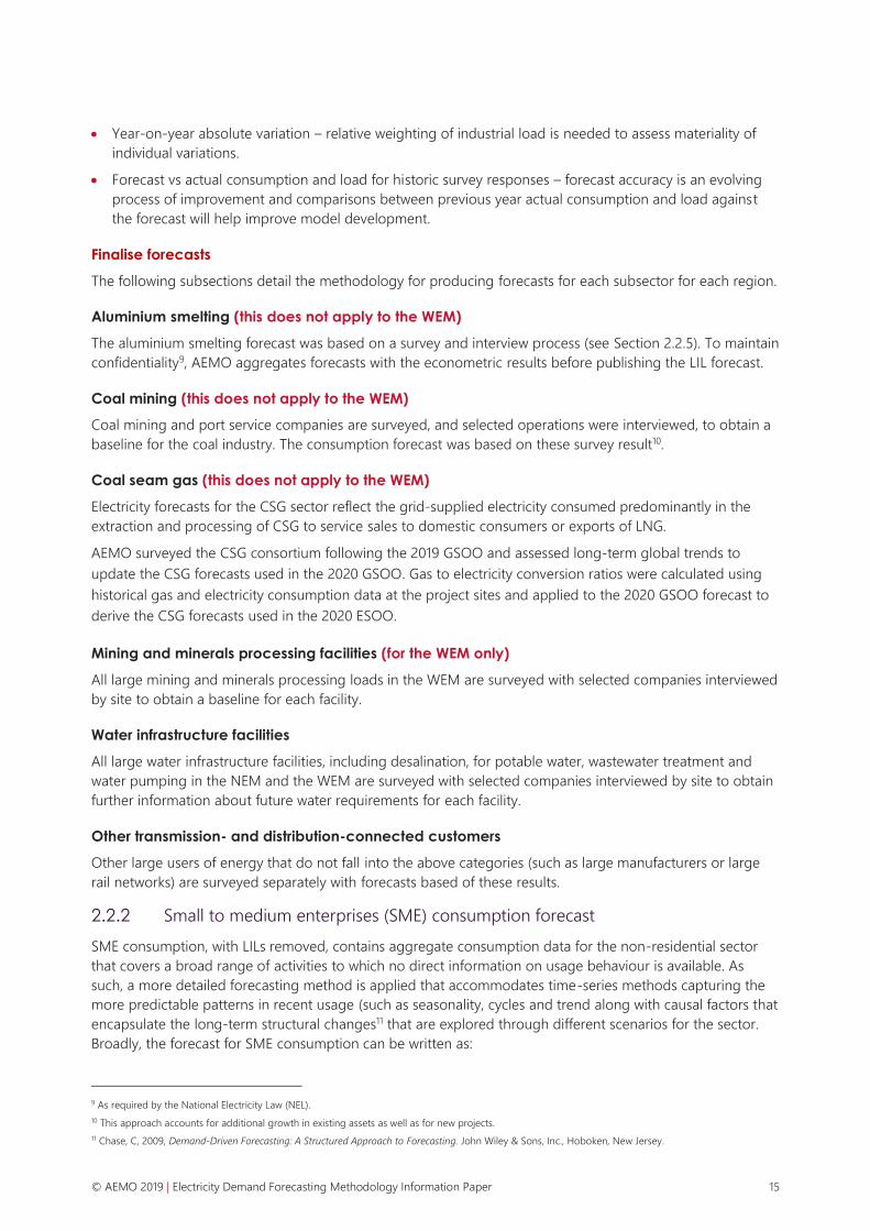
GSP Impact
The growth for the long-term SME forecast was developed using a linear regression model with ordinary least
squares to estimate coefficients16. The variables are described in Table 3 with subscript 𝑖 representing years
for the NEM and the WEM.
Table 3 SME model variable description
Variable names Abbreviation Units Description
SME consumption SME_Cons GWh SME business consumption.
Gross State Product GSP $ million
Real GSP is a measurement of the economic output of a state. It is the
sum of all value added by industries within the state.
* Coefficients for price elasticity for SME consumers were benchmarked against a broad literature review by AEMO.
Price impact
Adjustments are made to the forecast consumption to capture the negative impact of price increases. An
asymmetric response of consumers to price changes is used, with price impacts being estimated in the case
of increases, but not for price reductions.
Energy efficiency adjustment
AEMO engaged a consultant (in 2019, Strategy. Policy. Research. Pty Ltd) to develop forecasts of energy
efficiency savings for the Commercial and Industrial sectors. The 2020 energy efficiency adjustment is based
on the 2019 forecasts, updated with the latest input data on GSP, and the split between baseload, heating and
cooling load elements derived from meter data.
The forecasts estimate savings from a range of Federal and state government measures, including the
National Construction Code (NCC), building disclosure schemes, the Equipment Energy Efficiency (E3)
Program, and state schemes17. AEMO adjusted the forecasts to fit with the SME model by:
• Removing savings from Commercial and Industrial LILs18.
• Rebasing the consultant’s forecast to the SME model’s base year.
• Removing the estimated future savings from activities that took place prior to the base year.
• Extending the savings attributed to state schemes beyond legislated end dates, on the assumption that a
significant percentage (at least 75%) of activities would continue as business as usual depending on
scheme.
• Reviewing energy savings calculations for state schemes and where possible consulting with state
government departments.
AEMO applied a discount factor of approximately 20% to the adjusted energy efficiency forecasts, to reflect
the potential increase in consumption that may result from lower electricity bills. The discount factor also
reduces, in addition to steps taken by the consultant, the risk of overestimating savings from potential
double-counting and non-realisation of expected savings from policy measures.
16 These coefficients represent elasticity responses.
17 For 2019, the consultant modelled the NSW Energy Savings Scheme, Victorian Energy Upgrade Program, and the SA Retailer Energy Efficiency Scheme.
18 The consultant’s forecasts include savings from the LIL sector. AEMO surveys LILs separately and assumes that savings activities would be factored into the
consumption data obtained through the surveys, and as such removed LIL savings from the consultant’s forecasts.
𝑆𝑀𝐸_𝐶𝑜𝑛𝑠𝑖 = β̂0
+ β̂1
(𝐺𝑆𝑃𝑖)

© AEMO 2019 | Electricity Demand Forecasting Methodology Information Paper 19
For more details on trends and drivers on energy efficiency see the 2019 energy efficiency report produced by
Strategy. Policy. Research. Pty Ltd19.
Climate change adjustment
Heating and cooling load is expected to vary as the climate changes and the SME sector is adjusted to reflect
this. While the forecasts were produced assuming normalised weather standards, these standards evolve over
the forecast period due to climate change (see Appendix A2).
A climate change index was used to adjust heating and cooling load20 forecast for the SME sector.
The SME consumption, split into Heat, Base, and Cool elements for the base year, is then adjusted in
subsequent forecast years by the estimated climate change impact on the number of HDDs and CDDs.
Shock factor (structural break) adjustment
Economic shocks are noted to historically disrupt business activity and electricity consumption. For example
the Australian recession in 1990 and the Global Financial Crisis (GFC) in 2007 both resulted in reductions in
electricity consumption. The period after the GFC in particular, has been characterised by slower industrial
production output21.
AEMO has previously used factors to account for the disruption in long-term relationship with electricity
demand and economic indicators from the GFC. In 2020, due to the COVID-19 pandemic AEMO has applied a
shock-factor to the SME sector, to canvas the potential downside impact from the more energy-intensive
manufacturing sector.
The energy intensity of manufacturing was calculated by dividing the 2019 Department of Energy (Table F)
manufacturing sector annual electricity consumption by the actual 2019 manufacturing sector GVA provided
by AEMO’s economic consultant. Electricity consumption and GVA attributed to the aluminium sector was
removed prior to determining the energy intensity to mitigate overstating the size of the shock, as these
users are accounted for in the LIL forecasts. This factor was then multiplied by the forecast drop in GVA
between 2019 and 2021 from the economic forecast for each scenario (excluding Step Change) provided by
the economic consultant, producing the amount of load deemed at risk.
The impact was proportionally applied to the regional forecasts (based on the comparative size of each
regions’ manufacturing sector) with the size of the impact determined by the respective economic GVA
forecast for the manufacturing sector in each scenario. The shock factor was applied elastically in the Central
scenario, with the load returning after four years (a U-shaped recovery), while in the Slow Change scenario
the adjustment is applied with a proportion of load not being recovered (an L-shaped recovery), reflecting
the risk that some industrial consumption may not return.
Combining the short- and long-term models
There are several methods that can be used to combine different forecasting models. AEMO adopts a
weighted method for combining the forecast models; literature suggests an equal weight should apply where
there is uncertainty on what weights are appropriate.22 As the uncertainty of time-series methods increases as
the forecast horizon expands, yet time-series models are generally more accurate in the short-term, AEMO
has adopted an equal weighting of 50% for combing the short-term series model with the long-term causal
model (excluding the shock factor), in the first forecast year then decaying to 25% in the second forecast year,
12.5% in the third forecast year, then 0% afterwards, for the short-term component.
19 Strategy. Policy. Research. Pty Ltd. Energy Efficiency Forecasts: 2019 - 2041. July 2019, at https://www.aemo.com.au/-/media/Files/Electricity/NEM/
Planning_and_Forecasting/Inputs-Assumptions-Methodologies/2019/StrategyPolicyResearch_2019_Energy_Efficiency_Forecasts_Final_Report.pdf.
20 Heating load is defined as consumption that is temperature dependent (e.g. electricity used for heating). Load that is independent of temperature (e.g.
electricity used in cooking) is called Baseload or Non-heating load.
21 Langcake, S. Conditions in the Manufacturing Sector RBA Bulletin June Quarter 2016, at https://www.rba.gov.au/publications/bulletin/2016/jun/4.html.
22 Chase, C, 2009, Demand-Driven Forecasting: A Structured Approach to Forecasting. John Wiley & Sons, Inc., Hoboken, New Jersey.

© AEMO 2019 | Electricity Demand Forecasting Methodology Information Paper 20
The shock factor has been applied on top of the combined short and long-term models to preserve the
quantum of shocks forecast.
2.2.3 Electric vehicles
Projections for EV uptake and electricity consumption associated with electric vehicles were produced by
CSIRO23 in 2020. Charging of non-residential electric vehicles is considered to add to the consumption of the
SME category. For more detail refer to Appendix A4.
2.2.4 Battery storage loss adjustment
Battery losses were accounted-for by applying a round-trip efficiency of around 85% associated with the
utilisation of battery storage. For more details on trends and drivers see Appendix A3, and consultant reports,
the latest of which is by CSIRO24 and Green Energy Markets25.
2.2.5 Rooftop PV adjustment
This adjustment was made to translate energy consumption forecasts from an underlying consumption basis
to a delivered consumption basis. Underlying consumption refers to behind the meter consumption for a
business and does not distinguish between consumption met by energy delivered via the electricity grid or
generated from rooftop PV. Delivered consumption is the metered consumption from the electricity grid and
is derived by netting off rooftop PV generation from underlying consumption. For more details on trends and
drivers see the afore-mentioned consultant reports.
2.2.6 Total business forecasts
The aggregation of all sector forecasts is used to obtain the total business underlying consumption forecasts.
Total Business Underlying Consumption =
LIL consumption + SME consumption + Electric Vehicles consumption
Total business delivered consumption can be found as shown in Figure 5.
Figure 5 Aggregation process for final delivered forecast
23 CSIRO, 2020 projections for small-scale embedded technologies report, at https://aemo.com.au/-/media/files/electricity/nem/planning_and_forecasting/
inputs-assumptions-methodologies/2020/csiro-der-forecast-report.pdf?la=en.
24 CSIRO, 2020 projections for small-scale embedded technologies report, at https://aemo.com.au/-/media/files/electricity/nem/planning_and_forecasting/
inputs-assumptions-methodologies/2020/csiro-der-forecast-report.pdf?la=en.
25 GEM, 2020 Projections for distributed energy resources – solar PV and stationary energy battery systems report, at https://aemo.com.au/-/media/files/
electricity/nem/planning_and_forecasting/inputs-assumptions-methodologies/2020/green-energy-markets-der-forecast-report.pdf?la=en.

© AEMO 2019 | Electricity Demand Forecasting Methodology Information Paper 21
3. Residential annual consumption
This chapter outlines the methodology used in preparing residential annual consumption forecasts for each
NEM and WEM region.
3.1 Data sources
Residential consumption forecasts require large datasets to adequately represent the complex consumption
behaviours of residential users. Data sources are presented in Table 4 and Table 5.
Table 4 Historical input data sources for residential sector modelling
Data series Reference
Total daily residential connections for each region* AEMO metering database and from Synergy for the WEM.
Total daily underlying consumption for all residential customers for
each region**
AEMO metering database
Daily actual weather measured in HDD and CDD*** BoM temperature observations
* Daily residential connections were estimated by interpolating annual values.
** See Appendix A7 for more information
*** See Appendix A2 for more information
Table 5 Forecast input data sources for residential sector modelling
Data series Reference
Forecast annual HDD and CDD in standard weather conditions Appendix A2
Forecast annual residential connections Appendix A5
Forecast climate change impact on annual HDD and CDD Appendix A2
Forecast residential retail electricity prices Appendix A1
Forecast annual energy efficiency savings for residential base load,
heating and cooling consumption
Consultancy (Strategy. Policy. Research. Pty Ltd*in 2019)
Forecast gas to electric appliance switching 2020 GSOO**
Forecast annual rooftop PV generation Consultancy (CSIRO*** and Green Energy Markets**** in
2020) and Appendix A3

© AEMO 2019 | Electricity Demand Forecasting Methodology Information Paper 22
Data series Reference
Forecast electric appliance uptake Appendix A5
Forecast electric vehicles Consultancy (CSIRO in 2020)***
* Strategy. Policy. Research. Pty Ltd. Energy Efficiency Forecasts: 2019 - 2041. July 2019. Available at: https://www.aemo.com.au/-
/media/Files/Electricity/NEM/Planning_and_Forecasting/Inputs-Assumptions-
Methodologies/2019/StrategyPolicyResearch_2019_Energy_Efficiency_Forecasts_Final_Report.pdf
** AEMO 2019 Gas Demand Forecasting Methodology Information Paper. Available at: https://www.aemo.com.au/-
/media/Files/Gas/National_Planning_and_Forecasting/GSOO/2019/Gas-Demand-Forecasting-Methodology.pdf
*** CSIRO, 2020 projections for small-scale embedded technologies report, available at https://aemo.com.au/-
/media/files/electricity/nem/planning_and_forecasting/inputs-assumptions-methodologies/2020/csiro-der-forecast-report.pdf?la=en,
**** GEM, 2020 Projections for distributed energy resources – solar PV and stationary energy battery systems report, available at:
https://aemo.com.au/-/media/files/electricity/nem/planning_and_forecasting/inputs-assumptions-methodologies/2020/green-energy-
markets-der-forecast-report.pdf?la=en
3.2 Methodology
3.2.1 Process overview
AEMO applied a “growth” model to generate 20-year annual residential electricity consumption forecasts. At
the core of the forecast were the following stages:
• The average annual base load, heating load, and cooling load at a per-connection level were estimated.
This was based on projected annual heating degree days (HDD) and cooling degree days (CDD) under
‘standard’ weather conditions.
• The forecast then considered the impact of the modelled consumption drivers including electric appliance
uptake, energy efficiency savings, changes in retail prices, climate change impacts, gas-to-electricity
switching, and the rooftop PV rebound effect.
• The forecasts were then scaled up with the connections growth forecast to project future base, heating,
and cooling consumption by region over the forecast period26.
• The forecast of underlying residential consumption was estimated as the sum of base, heating, and
cooling load as well as the consumption from electric vehicles. The contribution from rooftop PV was then
subtracted to compute the forecast of delivered residential consumption, as well as adding back the losses
incurred in operating battery systems.
Figure 6 illustrates the steps undertaken to derive the underlying residential consumption forecast. Analysis of
the historical residential consumption trend is based on daily consumption per connection, on a regional
basis. The analysis conducted for each of these steps is discussed below.
26 The connection forecast methodology has been refined with a split of residential and non-residential connections. Only the residential connections are
used. For further information, see Appendix A5.

© AEMO 2020 | Electricity Demand Forecasting Methodology Information Paper 23
Figure 6 Process flow for residential consumption forecasts
000000000000000000
\
Electric Vehicles
Forecast
Annual Underlying & Delivered Residential Consumption
Apply trends and adjustments
Historical
Consumption per Connection
Annual Base Load Per Connection
Annual Cooling Load Per Connection
Annual Heating Load Per Connection
Forecast Connection Growth
Historical
HDD & CDD
Forecast
Annual Total Base Load Per Connection
Forecast
Annual Total Cooling Load Per Connection
Electric appliance uptake
Solar PV rebound effect
Consumer behavioural response to price changes
Energy efficiency savings
Climate change Weather normalise consumption per connection
split by base/heating/cooling loads
Annual HDD & CDD
Standard
Scale up base/heating/cooling loads with connection forecasts
Forecast
Annual Total Base Load
Forecast
Annual Total Heating Load
Forecast
Annual Total Cooling Load
Forecast
Annual Total Heating Load Per Connection
External driving factors
Solar PV Battery Losses

© AEMO 2020 | Electricity Demand Forecasting Methodology Information Paper 24
3.2.2 Model process
Step 1: Weather normalisation of residential consumption
Historical residential consumption was analysed to estimate average annual temperature-insensitive
consumption (base load) and average annual temperature-sensitive consumption in winter and summer
(heating load and cooling load) at a per-connection level. The estimates were independent of the impact
from year-to-year weather variability and the installed rooftop PV generation. The process is described in
more detail in the following steps. Due to the availability of data, the WEM applied the same model below
using monthly data. For this section, the subscript i for the WEM denotes month and the differences for the
WEM are outlined in brackets.
Step 1.1: Analyse historical residential consumption
Daily (monthly) average consumption per connection was determined by:
• Estimating the underlying consumption by removing the impact of rooftop PV generation (adding the
expected electricity generation from rooftop PV including avoided transmission and distribution network
losses from residential consumers to their consumption profile to capture all the electricity that the sector
has used, not just from the grid).
• Calculating the daily (monthly) average underlying consumption in each region.
• Estimating the daily (monthly) underlying consumption per residential connection by dividing by the total
connections.
A daily (monthly) regression model is used to calculate the daily (monthly) average consumption split
between baseload, cooling and heating load.
COVID-19 has altered the energy consumption pattern of the residential sector due to stay-at-home
restrictions and a higher utilisation of appliances in the home. In order to account for that AEMO has
introduced a dummy variable to canvas the impact of COVID-19 on the energy consumption of residential
sector.
Daily (monthly) regression model
Daily (monthly) consumption per connection was regressed against temperature measures (namely, CDD and
HDD) over a two-year window (training data) leading up to the reference year, using OLS estimates. The
window is chosen to reflect current usage patterns, e.g. the dwelling size and housing type mix but long
enough to capture seasonality in residential consumption. This model also has the capability to account for
other drivers impacting the consumption of the residential sector such as non-working days and COVID-19
period.
A similar regression approach was applied to all regions, except Tasmania (due to cooler weather conditions
in this region). The models are expressed as follows:
Regression model applied to all regions except Tasmania:
𝑅𝑒𝑠_𝐶𝑜𝑛𝑖,𝑡 = 𝛽𝐵𝑎𝑠𝑒,𝑖 + 𝛽𝐻𝐷𝐷,𝑖𝐻𝐷𝐷𝑖,𝑡 + 𝛽𝐶𝐷𝐷,𝑖𝐶𝐷𝐷𝑖,𝑡 + 𝛽𝑁𝑜𝑛−𝑤𝑜𝑟𝑘𝑑𝑎𝑦,𝑖𝑁𝑜𝑛_𝑤𝑜𝑟𝑘𝑑𝑎𝑦𝑖,𝑡
+ 𝛽𝐶𝑂𝑉𝐼𝐷−𝑖𝑚𝑝𝑎𝑐𝑡,𝑖𝐶𝑂𝑉𝐼𝐷_𝑖𝑚𝑝𝑎𝑐𝑡𝑖,𝑡 + 𝜀𝑖,𝑡
Regression model applied to Tasmania:
𝑅𝑒𝑠_𝐶𝑜𝑛𝑖,𝑡 = 𝛽𝐵𝑎𝑠𝑒,𝑖 + 𝛽𝐻𝐷𝐷,𝑖𝐻𝐷𝐷𝑖,𝑡 + 𝛽𝐻𝐷𝐷2,𝑖𝐻𝐷𝐷𝑖,𝑡2 + 𝛽𝑁𝑜𝑛−𝑤𝑜𝑟𝑘𝑑𝑎𝑦,𝑖𝑁𝑜𝑛_𝑤𝑜𝑟𝑘𝑑𝑎𝑦𝑖,𝑡
+ 𝛽𝐶𝑂𝑉𝐼𝐷−𝑖𝑚𝑝𝑎𝑐𝑡,𝑖𝐶𝑂𝑉𝐼𝐷_𝑖𝑚𝑝𝑎𝑐𝑡𝑖,𝑡 + 𝜀𝑖,𝑡
The above parameters were then used to estimate the sensitivities of residential loads per connection to
warm and cool weather.
For all regions (excluding Tasmania) this is expressed as:

© AEMO 2020 | Electricity Demand Forecasting Methodology Information Paper 25
𝐶𝑜𝑜𝑙𝑖𝑛𝑔𝐿𝑜𝑎𝑑𝑃𝑒𝑟𝐶𝐷𝐷𝑖 = 𝛽𝐶𝐷𝐷,𝑖
𝐻𝑒𝑎𝑡𝑖𝑛𝑔𝐿𝑜𝑎𝑑𝑃𝑒𝑟𝐻𝐷𝐷𝑖 = 𝛽𝐻𝐷𝐷,𝑖
For Tasmania this is expressed as:
𝐶𝑜𝑜𝑙𝑖𝑛𝑔𝐿𝑜𝑎𝑑𝑃𝑒𝑟𝐶𝐷𝐷𝑖 = 0
𝐻𝑒𝑎𝑡𝑖𝑛𝑔𝐿𝑜𝑎𝑑𝑃𝑒𝑟𝐶𝐷𝐷𝑖 =∑ (𝛽𝐻𝐷𝐷,𝑖 × 𝐻𝐷𝐷𝑡) + (𝛽𝐻𝐷𝐷2,𝑖 × 𝐻𝐷𝐷𝑡
2)𝑛𝑡=1
∑ 𝐻𝐷𝐷𝑡𝑛𝑡=1
Where 𝑛 is the total number of days in the two-year training data set.
Step 1.2: Estimate average annual base load, heating load and cooling load per connection,
excluding impacts from weather conditions and installed rooftop PV generation
𝐵𝑎𝑠𝑒𝑙𝑜𝑎𝑑_𝐶𝑜𝑛𝑖= 𝛽𝐵𝑎𝑠𝑒,𝑖 × 365
𝐻𝑒𝑎𝑡𝑖𝑛𝑔𝐿𝑜𝑎𝑑_𝐶𝑜𝑛𝑖= 𝐻𝑒𝑎𝑡𝑖𝑛𝑔𝐿𝑜𝑎𝑑𝑃𝑒𝑟𝐶𝐷𝐷𝑖 × 𝐴𝑛𝑛𝑢𝑎𝑙𝐻𝐷𝐷𝑖
𝐶𝑜𝑜𝑙𝑖𝑛𝑔𝐿𝑜𝑎𝑑_𝐶𝑜𝑛𝑖= 𝐶𝑜𝑜𝑙𝑖𝑛𝑔𝐿𝑜𝑎𝑑𝑃𝑒𝑟𝐶𝐷𝐷𝑖 × 𝐴𝑛𝑛𝑢𝑎𝑙𝐶𝐷𝐷𝑖
The variables of the model are defined in Table 6.
Table 6 Weather normalisation model variable description
Variable Description
𝑅𝑒𝑠_𝐶𝑜𝑛𝑖,𝑡 Daily average underlying consumption per residential connection for region i on day t
𝐻𝐷𝐷𝑖,𝑡 Average heating degree days for region i on day t
𝐶𝐷𝐷𝑖,𝑡 Average cooling degree days for region i on day t
𝐻𝐷𝐷𝑖,𝑡2 Square of average heating degree days for region i on day t which is to capture the quadratic
relationship between daily average consumption and HDD
𝑁𝑜𝑛 − 𝑤𝑜𝑟𝑘𝑑𝑎𝑦𝑖,𝑡 Dummy variable to flag a day-off for region i on day t. This includes public holidays and weekends.
𝐶𝑂𝑉𝐼𝐷_𝑖𝑚𝑝𝑎𝑐𝑡𝑖,𝑡 Dummy variable to flag COVID period for region i on day t.
𝐶𝑜𝑜𝑙𝑖𝑛𝑔𝐿𝑜𝑎𝑑𝑃𝑒𝑟𝐶𝐷𝐷𝑖 Estimated cooling load per CDD for region i.
𝐻𝑒𝑎𝑡𝑖𝑛𝑔𝐿𝑜𝑎𝑑𝑃𝑒𝑟𝐻𝐷𝐷𝑖 Estimated heating load per HDD for region i
𝐴𝑛𝑛𝑢𝑎𝑙𝐻𝐷𝐷𝑖 Projected annual HDD in standard weather conditions for region i
𝐴𝑛𝑛𝑢𝑎𝑙𝐶𝐷𝐷𝑖 Projected annual CDD in standard weather conditions for region i
𝐵𝑎𝑠𝑒𝑙𝑜𝑎𝑑_𝐶𝑜𝑛𝑖 Estimated average annual base load per connection for region i
𝐻𝑒𝑎𝑡𝑖𝑛𝑔𝑙𝑜𝑎𝑑_𝐶𝑜𝑛𝑖 Estimated average annual heating load per connection for region i
𝐶𝑜𝑜𝑙𝑖𝑛𝑔𝑙𝑜𝑎𝑑_𝐶𝑜𝑛𝑖 Estimated average annual cooling load per connection for region i
Step 2: Apply forecast trends and adjustments
The average annual base load, heating load and cooling load per connection estimated in Step 1 will not
change over the forecast horizon, being unaffected by the external driving factors. The adjustment that
accounts for external impacts, was performed in this second step.
For the purpose of forecasting changes to the annual consumption:

© AEMO 2020 | Electricity Demand Forecasting Methodology Information Paper 26
• Forecast residential retail prices are expressed as year-on-year percentage change.
• Forecast impact of annual energy efficiency savings, appliance uptake, and climate change are expressed
as indexed change to the reference year.
Step 2.1: Estimating the impact of electrical appliance uptake
The change in electrical appliance uptake is expressed using indices for each forecast year (set to 1 for the
reference year), for each region and split by base load, heating load and cooling load. The indices reflect
growth in appliance ownership, and also changes in the sizes of appliances over time (larger refrigerators and
televisions) and hours of use per year. Appliance growth is modified for policy-induced fuel switching from
gas to electrical appliances. See Appendix A5 for more detailed discussion of appliance uptake.
Certain appliances affect base load (such as fridges and televisions) while others are weather-sensitive (such
as reverse-cycle air-conditioners). The annual base load, heating load, and cooling load per connection is
scaled with the relevant indices to reflect the increase or decrease in consumption over time, relative to the
base year.
Step 2.2: Estimating the impact of solar PV rebound effect
It was assumed that households with installed rooftop PV are likely to increase consumption due to lower
electricity bills. The PV rebound effect was set equal to 20% of average forecast PV generation allocated
proportionally to base load, heating, and cooling load per connection.
Step 2.3: Estimating impact of climate change
The BoM and CSIRO assisted AEMO in understanding the impact of climate change on projected
temperatures. AEMO then adjusted the consumption forecast to account for the impact of increasing
temperatures (see Appendix A2 for more information). Climate change is anticipated to cause milder winters
and warmer summers which, as a result, reduce heating load while increasing cooling load in the forecast.
Due to the opposing effects of climate change on weather-sensitive loads, the annual net impact of climate
change can take a positive or negative value depending on which effect, on average, is larger.
Step 2.4: Estimating impact of consumer behavioural response to retail price changes
Changes in electricity prices have an impact on how consumers use electricity. Household response to price
change that was not captured by energy efficiency and rooftop PV was modelled through consumer
behavioural response. The asymmetric response of consumers to price changes is reflected in the price
elasticity estimation, with price impacts being estimated in the case of increases, but not for price reductions.
A price rise was estimated to have minimal impact on residential base load, which is largely from the
operation of appliances such as refrigerators, washing machines, microwaves, and lights. Hence, the price
elasticity for base load was set to be 0. For weather-sensitive loads, price elasticity was projected to be -0.1,
applied to both heating and cooling load per connection.
Step 2.5: Estimating impact of energy efficiency savings
Ongoing improvements in appliance efficiency and thermal performance of dwellings drive energy savings in
the residential sector. AEMO engaged a consultant (in 2019, Strategy. Policy. changes Research. Pty Ltd) to
forecast residential energy savings from a range of government measures, including the NCC, E3 program
and state schemes. Fuel switching between gas and electricity for space heating arising from changes to the
NCC is embedded in the EE forecasts and detailed in the consultant’s report27. Other fuel switching policies
are captured by the appliance growth indices.
The consultant apportioned energy savings by load segment using ratios developed by AEMO for each NEM
region, considering the total annual consumption that is sensitive to cool weather (heating load) and to hot
27 At https://www.aemo.com.au/-/media/Files/Electricity/NEM/Planning_and_Forecasting/Inputs-Assumptions-Methodologies/2019/StrategyPolicyResearch_
2019_Energy_Efficiency_Forecasts_Final_Report.pdf.

© AEMO 2020 | Electricity Demand Forecasting Methodology Information Paper 27
weather (cooling load). The residual consumption is considered temperature-insensitive and is apportioned to
baseload.
AEMO used the 2019 forecasts as the basis for the 2020 ESOO, including a discount factor (20%) on the
consultant’s forecast, and updated with the latest data on population growth, residential building stock
growth and National Meter Identifier (NMI) connections. See Appendix A5 for more detailed discussion on
the residential building stock model and NMI connections forecast.
Step 2.6: Estimating the forecasts of annual base load, cooling load and heating load per
connection accounting for external impacts
The forecasts of base load, heating load and cooling load per connection are then adjusted, considering the
impacts of external drivers estimated from Step 2.1 to 2.6. The external impacts are added to or subtracted
from the forecasts depending on how they affect each of the loads.
𝑇𝑂𝑇𝐵𝑎𝑠𝑒𝑙𝑜𝑎𝑑_𝐶𝑜𝑛𝑖,𝑗 = 𝐵𝑎𝑠𝑒𝑙𝑜𝑎𝑑_𝐶𝑜𝑛𝑖 + 𝐴𝑃𝐼_𝐵𝐿_𝐶𝑜𝑛𝑖,𝑗 + 𝑃𝑉𝑅𝐵_𝐵𝐿_𝐶𝑜𝑛𝑖,𝑗 − 𝐸𝐸𝐼_𝐵𝐿_𝐶𝑜𝑛𝑖,𝑗
𝑇𝑂𝑇𝐻𝑒𝑎𝑡𝑖𝑛𝑔𝑙𝑜𝑎𝑑_𝐶𝑜𝑛𝑖,𝑗
= 𝐻𝑒𝑎𝑡𝑖𝑛𝑔𝑙𝑜𝑎𝑑_𝐶𝑜𝑛𝑖 + 𝐴𝑃𝐼_𝐻𝐿_𝐶𝑜𝑛𝑖,𝑗 + 𝑃𝑉𝑅𝐵_𝐻𝐿_𝐶𝑜𝑛𝑖,𝑗 − 𝐸𝐸𝐼𝐻𝐿𝐶𝑜𝑛 𝑖,𝑗− 𝐶𝐶𝐼_𝐻𝐿_𝐶𝑜𝑛𝑖,𝑗
+ 𝑃𝐼_𝐻𝐿_𝐶𝑜𝑛𝑖,𝑗
𝑇𝑂𝑇𝐶𝑜𝑜𝑙𝑖𝑛𝑔𝑙𝑜𝑎𝑑_𝐶𝑜𝑛𝑖,𝑗
= 𝐶𝑜𝑜𝑙𝑖𝑛𝑔𝑙𝑜𝑎𝑑_𝐶𝑜𝑛𝑖 + 𝐴𝑃𝐼_𝐶𝐿_𝐶𝑜𝑛𝑖,𝑗 + 𝑃𝑉𝑅𝐵_𝐶𝐿_𝐶𝑜𝑛𝑖,𝑗 − 𝐸𝐸𝐼𝐶𝐿𝐶𝑜𝑛𝑖,𝑗+ 𝐶𝐶𝐼_𝐶𝐿_𝐶𝑜𝑛𝑖,𝑗
+ 𝑃𝐼_𝐶𝐿_𝐶𝑜𝑛𝑖,𝑗
Variables and their descriptions are detailed in Table 7.
Table 7 Variables and descriptions for residential consumption model
Variable Description
𝑇𝑂𝑇𝐵𝑎𝑠𝑒𝑙𝑜𝑎𝑑_𝐶𝑜𝑛𝑖,𝑗 Forecast total base load per connection for region i in year j
𝑇𝑂𝑇𝐻𝑒𝑎𝑡𝑖𝑛𝑔𝑙𝑜𝑎𝑑_𝐶𝑜𝑛𝑖,𝑗 Forecast total heating load per connection for region i in year j
𝑇𝑂𝑇𝐶𝑜𝑜𝑙𝑖𝑛𝑔𝑙𝑜𝑎𝑑_𝐶𝑜𝑛𝑖,𝑗 Forecast total cooling load per connection for region i in year j
𝐴𝑃𝐼_𝐵𝐿_𝐶𝑜𝑛𝑖,𝑗 Impact of electrical appliances uptake on annual base load per connection for region i in year j
𝐴𝑃𝐼_𝐻𝐿_𝐶𝑜𝑛𝑖,𝑗 Impact of electrical appliances uptake on annual heating load per connection for region i in year j
𝐴𝑃𝐼_𝐶𝐿_𝐶𝑜𝑛𝑖,𝑗 Impact of electrical appliances uptake on annual cooling load per connection for region i in year j
𝑃𝑉𝑅𝐵_𝐵𝐿_𝐶𝑜𝑛𝑖,𝑗 Impact of rooftop PV rebound effect on annual base load per connection for region i in year j
𝑃𝑉𝑅𝐵_𝐻𝐿_𝐶𝑜𝑛𝑖,𝑗 Impact of rooftop PV rebound effect on annual heating load per connection for region i in year j
𝑃𝑉𝑅𝐵_𝐶𝐿_𝐶𝑜𝑛𝑖,𝑗 Impact of rooftop PV rebound effect on annual cooling load per connection for region i in year j
𝐶𝐶𝐼_𝐻𝐿_𝐶𝑜𝑛𝑖,𝑗 Impact of climate change on average heating load per connection for region i in year j
𝐶𝐶𝐼_𝐶𝐿_𝐶𝑜𝑛𝑖,𝑗 Impact of climate change on average cooling load per connection for region i in year j
𝑃𝐼_𝐻𝐿_𝐶𝑜𝑛𝑖,𝑗 Impact of consumer behavioural response to price changes on annual heating load per connection for
region i in year j. This takes negative value, reflecting reduction in consumption due to price rises.
𝑃𝐼_𝐶𝐿_𝐶𝑜𝑛𝑖,𝑗 Impact of consumer behavioural response to price changes on annual cooling load per connection for
region i in year j. This takes negative value, reflecting reduction in consumption due to price rises.

© AEMO 2020 | Electricity Demand Forecasting Methodology Information Paper 28
Variable Description
𝐸𝐸𝐼_𝐵𝐿_𝐶𝑜𝑛𝑖,𝑗 Impact of energy efficiency savings on annual base load per connection for region i in year j
𝐸𝐸𝐼_𝐻𝐿_𝐶𝑜𝑛𝑖,𝑗 Impact of energy efficiency savings on annual heating load per connection for region i in year j
𝐸𝐸𝐼_𝐶𝐿_𝐶𝑜𝑛𝑖,𝑗 Impact of energy efficiency savings on annual cooling load per connection for region i in year j
Step 3: Scale by connections forecasts
Forecasts of annual base load, cooling load, and heating load at per connection level, after adjustment for
future appliance and technology trends, were then scaled up by connections forecast over the projection
period.
Forecasts of annual base load, heating load and cooling load were modelled as follows:
𝑇𝑂𝑇𝐵𝑎𝑠𝑒𝑙𝑜𝑎𝑑𝑖,𝑗 = 𝑇𝑂𝑇𝐵𝑎𝑠𝑒𝑙𝑜𝑎𝑑_𝐶𝑜𝑛𝑖,𝑗 × 𝑇𝑜𝑡𝑎𝑙𝑁𝑀𝐼𝑖,𝑗
𝑇𝑂𝑇𝐻𝑒𝑎𝑡𝑖𝑛𝑔𝑙𝑜𝑎𝑑𝑖,𝑗 = 𝑇𝑂𝑇𝐻𝑒𝑎𝑡𝑖𝑛𝑔𝑙𝑜𝑎𝑑_𝐶𝑜𝑛𝑖,𝑗 × 𝑇𝑜𝑡𝑎𝑙𝑁𝑀𝐼𝑖,𝑗
𝑇𝑂𝑇𝐶𝑜𝑜𝑙𝑖𝑛𝑔𝑙𝑜𝑎𝑑𝑖,𝑗 = 𝑇𝑂𝑇𝐶𝑜𝑜𝑙𝑖𝑛𝑔𝑙𝑜𝑎𝑑_𝐶𝑜𝑛𝑖,𝑗 × 𝑇𝑜𝑡𝑎𝑙𝑁𝑀𝐼𝑖,𝑗
Table 8 Residential base load, heating load and cooling load model variables and descriptions
Variable Description
𝑇𝑜𝑡𝑎𝑙𝑁𝑀𝐼𝑖,𝑗 Total connections for region i in year j
𝑇𝑂𝑇𝐵𝑎𝑠𝑒𝑙𝑜𝑎𝑑𝑖,𝑗 Forecast total base load for region i in year j
𝑇𝑂𝑇𝐻𝑒𝑎𝑡𝑖𝑛𝑔𝑙𝑜𝑎𝑑𝑖,𝑗 Forecast total heating load for region i in year j
𝑇𝑂𝑇𝐶𝑜𝑜𝑙𝑖𝑛𝑔𝑙𝑜𝑎𝑑𝑖,𝑗 Forecast total cooling load for region i in year j
Step 4: Estimate underlying and delivered annual consumption forecast
The forecast underlying annual consumption is expressed as the sum of base, heating and cooling loads and
residential electric vehicles, as shown in Figure 7.
Figure 7 Aggregation process for final residential underlying forecast
Total Residential Underlying Consumption Forecast
Total Residential Base Load
Total Residential Heating Load
Total Residential Cooling Load
Electric Vehicles
© AEMO 2020 | Electricity Demand Forecasting Methodology Information Paper 29
External advice is obtained from consultancies (in 2019 this was CSIRO and Energeia) for estimates of
historical and forecast electric vehicle uptake28.
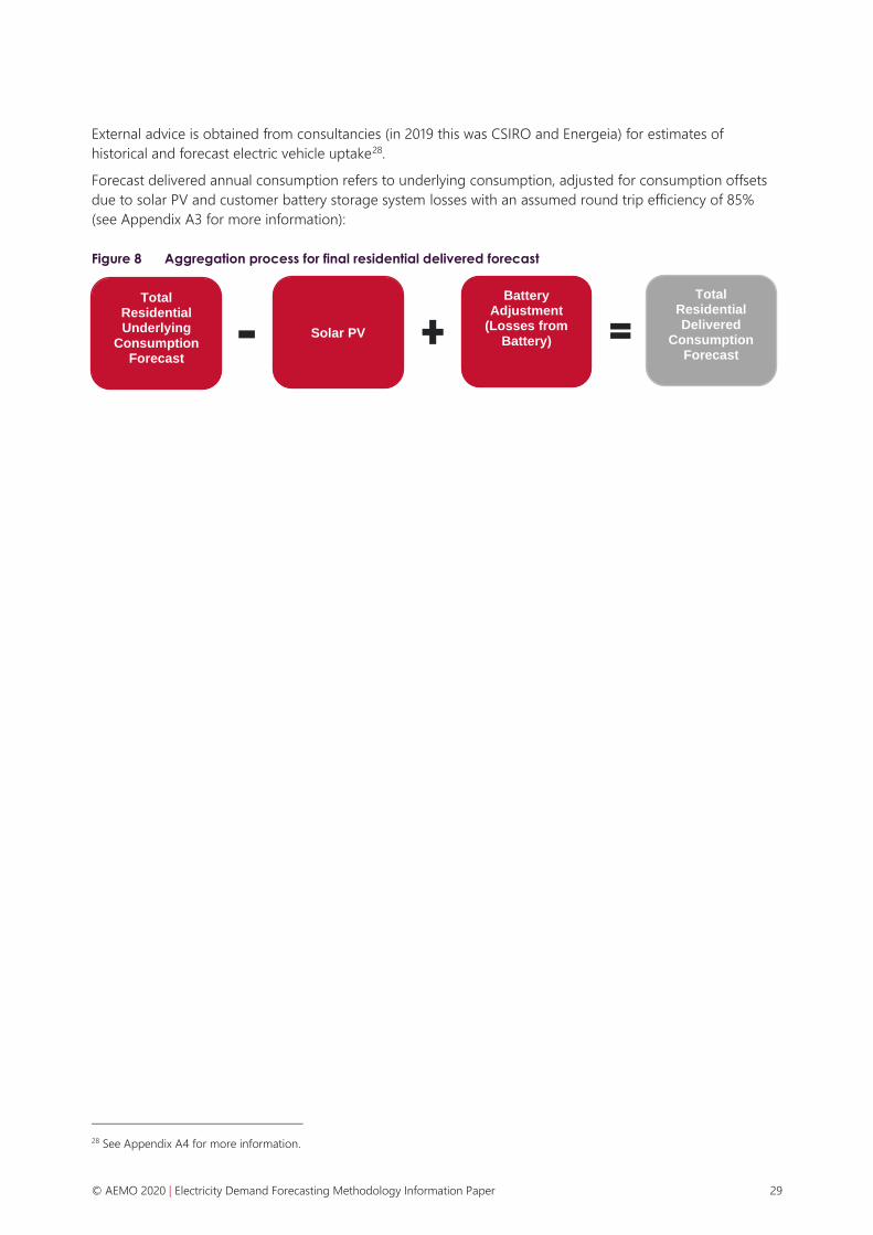
Forecast delivered annual consumption refers to underlying consumption, adjusted for consumption offsets
due to solar PV and customer battery storage system losses with an assumed round trip efficiency of 85%
(see Appendix A3 for more information):
Figure 8 Aggregation process for final residential delivered forecast
28 See Appendix A4 for more information.
Total Residential Underlying
Consumption Forecast
Solar PV
Battery Adjustment
(Losses from Battery)
Total Residential Delivered
Consumption Forecast

© AEMO 2020 | Electricity Demand Forecasting Methodology Information Paper 30
4. Operational consumption
AEMO forecasts operational consumption, representing consumption from residential and business
consumers, as supplied by scheduled, semi-scheduled and significant non-scheduled generating units29. The
remainder of non-scheduled generators are referred to as small non-scheduled generation (NSG). When
calculating operational consumption, energy supplied by small NSG was subtracted from delivered residential
and business sector consumption. Estimations of the transmission and distribution losses are added to the
delivered consumption to arrive at the operational consumption forecast.
Figure 9 Demand relationships
4.1 Small non-scheduled generation
This section discusses the methodology for PV non-scheduled generation (PVNSG) and Other non-scheduled
generation (ONSG).
4.1.1 Data sources
AEMO forecast small NSG based on the following data sources:
• Publicly available information.
• Data provided by network businesses.
• Projection of PV uptake (as forecast by the consultants, in 2020 CSIRO and Green Energy Markets).
29 Operational definition at https://aemo.com.au/-/media/files/stakeholder_consultation/consultations/nem-consultations/2019/dispatch/demand-terms-in-
emms-data-model---final.pdf.
© AEMO 2020 | Electricity Demand Forecasting Methodology Information Paper 31
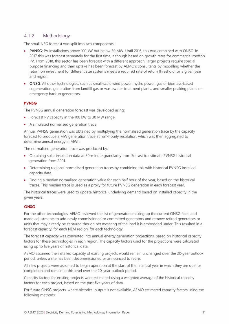
4.1.2 Methodology
The small NSG forecast was split into two components:
• PVNSG: PV installations above 100 kW but below 30 MW. Until 2016, this was combined with ONSG. In
2017 this was forecast separately for the first time, although based on growth rates for commercial rooftop
PV. From 2018, this sector has been forecast with a different approach; larger projects require special
purpose financing and their uptake has been forecast by AEMO’s consultants by modelling whether the
return on investment for different size systems meets a required rate of return threshold for a given year
and region.
• ONSG: All other technologies, such as small-scale wind power, hydro power, gas or biomass-based
cogeneration, generation from landfill gas or wastewater treatment plants, and smaller peaking plants or
emergency backup generators.
PVNSG
The PVNSG annual generation forecast was developed using:
• Forecast PV capacity in the 100 kW to 30 MW range.
• A simulated normalised generation trace.
Annual PVNSG generation was obtained by multiplying the normalised generation trace by the capacity
forecast to produce a MW generation trace at half-hourly resolution, which was then aggregated to
determine annual energy in MWh.
The normalised generation trace was produced by:
• Obtaining solar insolation data at 30-minute granularity from Solcast to estimate PVNSG historical
generation from 2001.
• Determining regional normalised generation traces by combining this with historical PVNSG installed
capacity data.
• Finding a median normalised generation value for each half hour of the year, based on the historical
traces. This median trace is used as a proxy for future PVNSG generation in each forecast year.
The historical traces were used to update historical underlying demand based on installed capacity in the
given years.
ONSG
For the other technologies, AEMO reviewed the list of generators making up the current ONSG fleet, and
made adjustments to add newly commissioned or committed generators and remove retired generators or
units that may already be captured though net metering of the load it is embedded under. This resulted in a
forecast capacity, for each NEM region, for each technology.
The forecast capacity was converted into annual energy generation projections, based on historical capacity
factors for these technologies in each region. The capacity factors used for the projections were calculated
using up to five years of historical data.
AEMO assumed the installed capacity of existing projects would remain unchanged over the 20-year outlook
period, unless a site has been decommissioned or announced to retire.
All new projects were assumed to begin operation at the start of the financial year in which they are due for
completion and remain at this level over the 20-year outlook period.
Capacity factors for existing projects were estimated using a weighted average of the historical capacity
factors for each project, based on the past five years of data.
For future ONSG projects, where historical output is not available, AEMO estimated capacity factors using the
following methods:

© AEMO 2020 | Electricity Demand Forecasting Methodology Information Paper 32
• Where similar projects already exist, in terms of NEM region and generator class (fuel source), AEMO used
the total historical output from all similar, existing projects, divided by their combined rated capacity.
• Where no similar projects exist typically a new generator class in a particular NEM region, AEMO either
used the regional average for all existing generators or applied the capacity factor of similar generators
from another region.
AEMO then combined the resulting capacity factor profile with the expected capacities of all future generator
projects and used this to forecast the expected generation per project over the outlook period.
4.2 Network losses and auxiliary loads
4.2.1 Network losses
Transmission losses forecast methodology
Transmission losses represent energy lost due to electrical resistance and the heating of conductors as
electricity flows through the transmission network.
The Australian Energy Regulator (AER) and the network operators provide AEMO with historical transmission
loss factors. AEMO uses the transmission loss factors to calculate historical losses across the transmission
network for each region.
AEMO forecasts annual transmission losses by using the historical normalised transmission losses averaged
over the last five years. Annual transmission losses were normalised by electricity consumption by large
industrial customers as well as residential and commercial customers.
Distribution losses
To calculate operational demand from estimated delivered demand, distribution losses are needed in
addition to transmission losses. The distribution losses were estimated as a volume weighted average per
region, generally based on recent losses reported to the AER by distribution companies as part of the
Distribution Loss Factor approvals process.
4.2.2 Auxiliary loads methodology
Auxiliary loads account for energy used within power stations (the difference between “as generated” energy
and “sent-out” energy).
Auxiliary loads (historical)
Analysis for auxiliary loads requires historical data obtained from the wholesale market system – Market
Management System (MMS). Auxiliary loads are not directly measured and so are modelled with the
assumption that they are equal to the difference between total generation as measured at generator
terminals and the electricity that is sent out into the grid. The amount of energy that is sent out to the grid is
estimated by multiplying the metered generation for an individual generating unit by using an estimated
auxiliary percentage30 for the generation station such that:
Auxiliary Load = Metered Generation x Auxiliary Percentage
For example, a new combined cycle gas turbine has an assumed auxiliary factor of 3%, such that if the
metered generation in a day was 30 MWh will have a calculated auxiliary load of 0.9 MWh. The sent out
energy for this power station is therefore determined to be 29.1 MWh.
This method is applied for approximately 250 generating units in the NEM to arrive at the calculated historical
auxiliary load and operational demand as sent out on a half hourly basis.
30 See https://www.aemo.com.au/-/media/Files/Electricity/NEM/Planning_and_Forecasting/Inputs-Assumptions-Methodologies/2019/2019-Input-and-
Assumptions-workbook.xlsx.

© AEMO 2020 | Electricity Demand Forecasting Methodology Information Paper 33
Auxiliary loads (forecast)
The annual auxiliary loads in each region were forecast using the auxiliary loads from a future generation
forecast that have a mix of technologies. Forecasts of the future generation mix are currently based on the
2020 Integrated System Plan (ISP) auxiliary load forecasts with each of the 2020 scenarios modelled in the ISP.
As the 2020 ISP was based on earlier consumption forecasts than the 2020 forecasts (broadly based on 2019
forecasts, but for one Updated Demand sensitivity), they needed to be rebased to preserve the auxiliary load
proportion of energy consistent with the 2020 ESOO forecasts. To arrive at this adjustment, the forecast
auxiliary factor for each financial year and for each NEM region in the 2020 ESOO was defined as:
Auxiliary Load Factor (2020 ESOO) =Total Auxiliary Load (ISP)
Operational Consumption Forecast as sent out (ISP)
The annual auxiliary load forecast was then determined by first calculating the operational consumption
forecast (as generated) by dividing the 2020 ESOO operational consumption forecast (as sent-out) by the
2020 ESOO Auxiliary Load Factor. The auxiliary load forecast is then the difference between the operational
consumption forecast (as generated) and the operational forecast (as sent out).

© AEMO 2020 | Electricity Demand Forecasting Methodology Information Paper 34
5. Maximum and minimum demand
Regional minimum and maximum demand forecasts are developed by season using a probabilistic
methodology. Demand is dependent on both structural drivers as well as random drivers including weather
conditions, seasonal effects and random stochastic volatility.
To model this uncertainty, several scenarios are developed to capture uncertainty in structural drivers, while
uncertainty attributable to random drivers is expressed as an interval, probability of exceedance (POE)
forecast from a forecast distribution. As such, forecast maximum demand (MD) is not a single point forecast.
For any given season or year:
• A 10% POE MD value is expected to be exceeded, on average, one year in 10.
• A 50% POE MD value is expected to be exceeded, on average, one year in two.
• A 90% POE MD value is expected to be exceeded, on average, nine years in 10.
Figure 10 shows modelled probability density functions that represent possible maximum demand outcomes
for a typical southern region. Three probability density functions are shown, one for each of the scenarios
with unique structural drivers. The 10% probability of exceedance (POE) estimates are sampled from the
probability distributions, shown by the vertical lines.
Figure 10 Conceptual summer maximum demand probability density functions for three scenarios
For the purpose of forecasting demand, AEMO defined summer as the period from November to March
(inclusive) except for Tasmania where summer was defined as the period from December to February
(inclusive). Winter was defined as being from June to August for all jurisdictions.
AEMO forecasts unconstrained maximum and minimum demand. That is, demand that is unconstrained by
subregional network constraints, generation constraints or outages, wholesale market dynamics and demand
side participation.

© AEMO 2020 | Electricity Demand Forecasting Methodology Information Paper 35
AEMO forecasts operational demand ‘sent out’ as defined in Section 1.3. In the following it will be referred to
as OPSO. Based on estimates of auxiliary load, this can be converted into forecast operational ‘as generated’
(OPGEN) maximum and minimum demand.
Maximum demand is forecast as Season Year to prevent any of the seasons (summer/winter) being arbitrarily
split by the year definition. Season Year is from 1 September to 30 August. For instance, 1 September 2018 to
30 August 2019 would be season year 2019.
The WEM maximum demand is forecast based on capacity year which is from 1 October to 30 September the
following year.
5.1 Data preparation
Data preparation for both the minimum and maximum demand models was similar to the requirements for
annual consumption, however each requires the use of half-hourly data. The requirement for
higher-frequency data drives the need for more thorough data cleaning and to consider the daily shape of
small-scale technologies and large industrial loads.
At a half-hour frequency by region the following data inputs were used:
• Historical and forecast rooftop PV capacity and normalised generation.
• Historical and forecast PVNSG installed capacity and normalised generation.
• Forecast electric vehicles numbers and charge profile.
– A proportion of EV is considered using coordinated charging with the proportion varying by scenario.
• Forecast ESS installed capacity and charge/discharge profile.
– A proportion of ESS is considered virtual power plant (VPP) or distributed energy resource (DER) with
the proportion varying by scenario.
• NMI data for the top 100 large industrial loads (loads over 10 MW, 10% of the time).
• Historical and forecast LILs.
• Historical underlying demand.
• Projected climate change adjusted dry temperature.
AEMO sourced half-hourly weather data from the BoM for the weather stations listed in Appendix A.2. The
weather data was climate change-adjusted for temperatures expected in the forecast horizon based on
information available on www.climatechangeinaustralia.gov.au.
The model aimed to generate forecasts of underlying demand less large industrial load. Large industrial load
was subtracted from underlying demand before constructing the model. Large industrial load may be
seasonal but is not considered to be weather-sensitive, although it can have the potential to cause structural
shifts in demand.
5.2 Exploratory data analysis
Exploratory data analysis (EDA) was used to detect outliers and identify important demand drivers and
multicollinearity during model development.
5.2.1 Outlier detection and removal
Outlier detection procedures were used to detect and remove outliers caused by data errors and outages. A
basic linear model was specified to examine all observations greater than more than three standard
deviations from the predicted value at each half-hour.
© AEMO 2020 | Electricity Demand Forecasting Methodology Information Paper 36
The resulting list of outliers and the known list of network outages were used to remove these data points to
constrain the dataset. Any data errors detected through this process were tracked to determine cause
followed by appropriate data corrections. No data was removed unless there was cause to remove it, because
by definition maximum demand is an outlier more than three standard deviations from the mean and the
purpose is not to remove legitimate data. No augmentation of data was performed for missing data.
5.2.2 EDA to identify important short-term demand drivers
EDA was used to identify key variables that drive demand over the course of the year, by examining summary
statistics of each variable, correlations between explanatory variables to identify multicollinearity, and
correlations between explanatory variables and demand.
Broadly, the EDA process examined:
• Weather data – temperature variables including:
– Instantaneous cooling degree (CDs) and heating degree (HDs).
– Dry bulb temperature – both instantaneous and heatwave/coolwave.
– ‘Instantaneous’ temperature may be transformed as half-hourly up to three hour rolling average of
temperature.
– ‘Heatwaves’ and ‘coolwaves’ as daily up to three day rolling average of temperature.
○ Heatwaves were collinearly related with temperature variables derived from humidity. To avoid
multicollinearity, the heatwave variables were retained, and the temperature variables derived
from humidity were dropped.
– Apparent temperature31 – both instantaneous and heatwave/coolwave.
– EHF – excess heating factor is a measure of heatwave intensity. When maximum daily temperatures are
above the 95th percentile32 for three consecutive days, then these days are deemed to be in heatwave
conditions with the variable increasing with the intensity.
– Heat index33 – both instantaneous and heatwave.
– Higher order terms of the above variables, for example 𝐼𝑛𝑠𝑡𝑎𝑛𝑡Temperature2 and
𝐷𝑎𝑖𝑙𝑦𝑇𝑒𝑚𝑝𝑒𝑟𝑎𝑡𝑢𝑟𝑒2, to capture changing dynamics between temperature and demand at different
ends of demand.
• Calendar/seasonal variables, including weekday/weekend and public holiday Boolean (true/false) variables.
The Calendar/seasonal variables and other indicator variables in practise work to stratifies the data in different
seasons, weekends and weekdays. The fixed effects model effectively models different seasons, months,
weekdays and hours separately within the same model.
The EDA process assessed multicollinearity of the explanatory variables by consider the Variance Inflation
Factor34 caused by collinear variables.
5.3 Model development and selection
AEMO developed three models for each region, a half-hourly model, a maximum Generalized Extreme Value
(GEV) model and a minimum GEV model. Models for each region were specified using the variables identified
as statistically significant during the EDA process.
31 Measures the temperature perceived by humans. Ii is a function of dry bulb air temperature, relative humidity and wind speed.
32 The 95th percentile on the daily maximum temperature for that weather station in the region.
33 Measures the perception of temperature above 27 degrees. It is a function of dry bulb air temperature and humidity.
34 The variance inflation factor is a measure of multicollinearity between the explanatory variables in the model. Multicollinearity occurs when multiple
explanatory variables are linearly related and is undesirable because it could have the effect of increasing the variance of the model.

© AEMO 2020 | Electricity Demand Forecasting Methodology Information Paper 37
The half-hourly models simulate half-hourly demand and perform well in modelling the impact of disruptive
technology such as PV, ESS and EV. These technologies have a half-hourly shape and cause demand to shift
over the day. The GEV models are seasonal (or monthly) minimum and maximum models that produce
interval forecasts for minimum and maximum demand. AEMO used the GEV models to estimate the intervals
of minimum and maximum demand in the first year of the forecast. Then AEMO used the half-hourly model
to grow demand out 20 or 30 years.
Half-hourly model
The half hourly models aimed to describe the relationship between underlying demand and key explanatory
variables including calendar effects such as public holidays, day of the week and month in the year as well as
weather effects (such as 𝐼𝑛𝑠𝑡𝑎𝑛𝑡Temperature, and 𝐼𝑛𝑠𝑡𝑎𝑛𝑡Temperature2 and daily rolling average of
temperature).
AEMO used a Machine Learning algorithm to derive a model with good fit and strong predictive power. The
Least Absolute Shrinkage and Selection Operator (LASSO)35 regularization algorithm, a special case of Elastic
Net, selects the best model from the range of variables available and all the interactions between the
variables. The model was developed trading off the model bias36 and model variance37 to derive a
parsimonious model with strong explanatory power.
AEMO then performed additional in-sample and out-of-sample model diagnostic checks on the best model
selected by LASSO. Where the best model failed these checks AEMO adjusted the LASSO algorithm
iteratively. AEMO:
• Performed k-folds out-of-sample cross validation38 to find the optimal model that trades off between bias
and variance.
• Inspected the QQ-plots, the residual diagnostics over time and against the x variables to ensure the
residuals were random with no discernible patterns that could indicate missing explanatory factors.
• Inspected residuals at the relevant ends of demand to ensure that the assumptions for residuals when
simulating minimum and maximum demand are relevant and that there is no bias at either ends of
extreme demand.
• Compared actual against predicted from the half-hourly model.
• Compared actual detrended historical minima and maxima against simulated minima and maxima from
the model.
Table 9 details the variables selected as important in the EDA process after rejecting the other variables for
reason of weak correlation with demand or multicollinearity with other explanatory variables. In the case of
multicollinearity, the EDA process opted for simplicity by selecting more easily understood variables such as
dry temperature rather than derived weather variables such as apparent temperature. These variables were
then used in the final half-hourly demand model.
Table 9 List of variables included for half-hourly demand model
Variable Description
Public holiday Dummy flag for public holiday
Half-hour factor A factor variable with values for each half hour of the day
35 AEMO fit the LASSO regularization path for linear regression using cyclical coordinate descent in a path-wise fashion.
36 Under-fitting the model results in a model with high bias.
37 Over-fitting the model result in a model with high variance.
38 A 10-fold cross validation was performed by breaking the data set randomly into 10 smaller sample sets (folds). The model was trained on 9 of the folds
and validated against the remaining fold. The model was trained and validated 10 times until each fold was used in the training sample and the validation
sample. The forecast accuracy for each fold was calculated and compared between models.

© AEMO 2020 | Electricity Demand Forecasting Methodology Information Paper 38
Variable Description
Weekend dummy Dummy flag for weekend
Month factor A factor variable with values for each months of the year
temperature Transformation of dry temperature ie rolling average, weekly average, daily average or half-hourly as well as
quadratic or cubic transformation depending on model fit.
Generalise extreme value model
AEMO specified a separate model for minimum and maximum demand. The GEV is based on extreme value
theory to capture the distribution of rare events or the limit distribution of normalized minima and maxima.
The GEV model aimed to model the distribution of extreme values (minima and maxima) for operational
demand less large industrial load. As such the extreme value model was trained on weekly operational
minima and maxima less large industrial loads.
The GEV models found the relationship between minimum and maximum demand and PV Capacity, PVNSG
capacity and weekly weather metrics. AEMO developed the GEV models by iteratively selecting variables to
explain demand and testing the performance of the model through in-sample and out-of-sample diagnostics.
The explanatory variables are detailed in Table 10. The GEV model was fit using weekly operational minima
and maxima as a function of PV capacity, PVNSG capacity, customer number count (NMIs), calendar effect
variables and average weather. Similar to the half-hourly model, AEMO then assessed the in-sample
performance by:
• Inspecting the QQ-plot, the residual diagnostics over time and explanatory power of the x variables to
ensure the residuals were random with no discernible patterns that could indicate missing explanatory
factors, and
• Inspecting that degree of serial correlation in the residuals, where no serial correlation is desired.
Finally, AEMO assessed the out-of-sample performance by comparing:
• Actual against predicted from the GEV model, and
• Actual historical minima and maxima against simulated minima and maxima from the GEV models.
Table 10 List of variables included for half-hourly demand model
Variable Description
Month factor A factor variable with values for each months of the year
PV capacity The sum in MW of the all the rooftop PV panels in a region
PVNSG capacity The sum in MW of the all the PV non-scheduled generators in a region
NMI count The number of NMIs within a region
Dry temperature Transformation of dry temperature ie rolling average, weekly average, daily average or half-hourly
as well as quadratic or cubic transformation depending on model fit.
Solar irradiance Some transformation of Solar irradiance ie rolling average, weekly average, daily average or half-
hourly depending on model fit

© AEMO 2020 | Electricity Demand Forecasting Methodology Information Paper 39
5.4 Simulate base year (weather and calendar normalisation)
The half-hourly and GEV models selected from the above process were used to simulate demand for each
region. All three models were used to simulate, the half-hourly models were used to simulate every half-hour
hour and aggregate to the season. The GEV models were used to simulate minima and maxima for each
week which were aggregate to the season. Such that for each season and region we had minima and maxima
from the half-hourly model and minima and maxima from the GEV models (two set of minima and maxima).
The GEV was used for the first forecast year then transitioned to the half-hourly model for the long-term
forecast horizon.
Demand was simulated using calendar effects, stochastic volatility and weather. Historical weather events
were simulated to develop a weather distribution to normalise demand then stochastic volatility was applied:
𝑈𝑛𝑑𝑒𝑟𝑙𝑦𝑖𝑛𝑔ℎℎ = 𝑓(𝑥ℎℎ) + 𝜀ℎℎ
𝑀𝑎𝑥𝑂𝑝𝑠𝑜𝑤𝑒𝑒𝑘 = 𝑓(𝑥𝑤𝑒𝑒𝑘) + 𝑔(𝑥𝑤𝑒𝑒𝑘) + 𝜇3 + 𝜀𝑤𝑒𝑒𝑘
𝑀𝑖𝑛𝑂𝑝𝑠𝑜𝑤𝑒𝑒𝑘 = 𝑓(𝑥𝑤𝑒𝑒𝑘) + 𝑔(𝑥𝑤𝑒𝑒𝑘) + 𝜇3 + 𝜀𝑤𝑒𝑒𝑘
Where:
• 𝑓(𝑥ℎℎ) is the relationship between demand and the demand drivers such as weather and calendar effects.
• 𝑓(𝑥𝑤𝑒𝑒𝑘) is the relationship between weekly minima/maxima demand and the weekly demand drivers such
as PV or PVNSG capacity and NMI count.
• 𝑔(𝑥𝑤𝑒𝑒𝑘) the second moment scale parameter as a function of x variables.
• 𝜇3 the third moment shape parameter which was found to be a constant.
• 𝜀ℎℎ represents random normally distributed39 changes in demand not explained by the model demand
drivers.
• 𝜀𝑤𝑒𝑒𝑘𝑙𝑦 represents random normally distributed39 changes in demand not explained by the model demand
drivers from the GEV models.
Half-hourly model simulation
The weather was simulated for the base year by block bootstrapping historical weather observations (𝑥ℎℎ) to
create a year consisting of 17,520 half-hourly weather observations. A synthetic weather-year was constructed
by randomly selecting 26 fortnightly weather patterns (“weather blocks”) and stitching together the 26
fortnights to construct one weather year. The fortnights were stitched together in order to ensure that they
corresponded to the correct time of year, summer fortnights to summer and winter fortnights to winter.
The weather data was block bootstrapped from 20 historical weather years warmed to future climates40. A
total of 3,000 weather simulations were created to derive 3,000 weather years of data (at half-hourly
observations)41.
The weather blocks were spliced together from midnight to midnight 14 days after. No attempt was made to
smooth the joins between the fortnights. Only a given half-hour is considered in the context of minimum and
maximum demand not the full time-series or the shape of the data.
The above mentioned half-hourly models were used to estimate demand for the given conditions of a
synthetic year, which accounts for the correlation between demand and the conditions implied by the
models. Simultaneously, the stochastic volatility was simulated to account for the component of demand
39 A fundamental assumption of Ordinary Least Squares (OLS) is that the error term follows a normal distribution. This assumption was tested using graphical
analysis and the Jarque–Bera test.
40 Bootstrapping with replacement preserves empirical correlations between time-of-year, temperature, and solar irradiance time series.
41 Previous tests indicate that 500 Monte Carlo simulations is a sufficient number of simulations to converge to a stable result that varies around half a
percent in the early years, while 1000 simulations reduce the variability to about 0.3% in the early years. Variability does increase in the later years of the
forecast horizon.

© AEMO 2020 | Electricity Demand Forecasting Methodology Information Paper 40
variability unexplained by other demand drivers captured in the models (𝜀ℎℎ) which is a feature of all
statistical models. The synthetic half-hourly demand traces were estimated for 3,000 simulated years.
The simulation process recognised that there are several drivers of demand including weather, day of week,
and hour of day, as well as the natural stochastic volatility of a statistical model. The process also preserved
the probabilistic relationship between demand and its key drivers.
GEV model simulation
The GEV model was simulated in a similar process as the half-hourly model. However, the GEV model is less
reliant on weather and is more reliant on capturing and understanding the distribution of the extreme values.
The simulation process constructed synthetic weather years by sampling daily weather data from history.
While the GEV model was specified as a weekly model, daily data was used to increase the number of
simulations. The GEV model was then applied to the synthetic weather years to estimate the point forecast
component of the GEV.
The GEV distribution was simulated using the same synthetic weather years. In the GEV model the variance of
the model is a function of the x variables. The variance of the GEV model was simulated using the x variables
from the synthetic weather years.
Finally, the simulation process simulated random normally distribution stochastic volatility of demand. The
stochastic volatility was simulated to account for the component of demand variability unexplained the
demand drivers captured in the linear model (𝜀ℎℎ) which is a feature of all statistical models.
5.5 Forecast probability of exceedance for base year
The GEV simulation estimates demand for the base year of the forecast. The base year of the ESOO MD
demand forecast is the last year of summer actuals. For instance, if the last summer actual demand was
31 March 2019, then base year for the purpose of the forecast is financial year end 2019.
The minimum and maximum demand values were pulled for each synthetic weather year of the GEV
simulation. Then the distribution of the minima and maxima was established to calculate the probability of
exceedance for operational demand for the base year of the forecast.
5.6 Forecast probability of exceedance for long term
Once the base year was established from the GEV simulation, the half-hourly model then forecast the
year-on-year change in demand accounting for shifts in time of day for minimum and maximum demand.
The half-hourly forecast process grows half-hourly demand by economic conditions such as price and GSP,
demographic conditions such as connections growth, and technological conditions such as electric vehicle
uptake to derive an annual growth index.
The forecast year-on-year change was applied to each of the 17,520 half-hours for each simulation in the
half-hourly model and to each forecast year. The process grows half-hourly underlying demand by annual or
seasonal growth indices such as population growth, economic factors and price.
This process yields demand values for each half-hour over a simulated year. This represents the half-hourly
prediction of the 17,520 half-hours forecast in a given year, for each year in the forecast horizon. The
prediction values, as explained previously, represent Underlying demand less LIL.
At this point, the process converts this to operational demand ‘sent out’ and ‘as generated’. This is done
by subtracting other forms of generation (rooftop PV, PVNSG and ONSG), adjusting for daily profiles for ESS
and EV operation, and adding LIL, distribution and transmission losses back on. As a result, the load factor
between maximum demand and annual energy changes over time. For more information on translating
Underlying demand to Operational demand, see Figure 3 in Section 1.3.

© AEMO 2020 | Electricity Demand Forecasting Methodology Information Paper 41
See below for more information on the LIL, losses, ONSG and auxiliary (needed for ‘as generated’) forecasts
at time of minimum and maximum demand.
AEMO then extract the seasonal minima and maxima from the simulations. The number of simulations is
chosen to be large enough to obtain a smooth distribution of predictions, subject to computational resource
limits. For example, if 3,000 simulations are performed, there will be 3,000 maximum and 3,000 minimum
values for each scenario-season-year combination. From the 3,000 simulated minima/maxima, AEMO then
extracts the necessary POE levels as well as the characteristics at times of the minimum/maximum (such as
weather conditions and calendar positioning at the time of minimum/maximum).
In Figure 11:
• The first distribution represents the variability of 17,520 half-hour demand for each simulation. This is
obtained for all years needed to produce a forecast year. Data for one half-hour representing the largest
predicted MD (indicated by the red box and arrow) was then extracted from the 17,520 half-hours and
added to the distribution of annual maxima (represented by the smaller bell curve). This extraction was
repeated 1,000 times, once for each simulation.
• The second smaller bell curve represents the distribution of maxima which may or may not be normally
distributed42.
AEMO extracts minimum/maximum values by region from this minima/maxima distribution by selecting the
10th, 50th and 90th percentile as 90%, 50% POE and 10% POE values, respectively.
Figure 11 Theoretical distribution of annual half-hourly data to derive maxima distribution
AEMO then transitioned from the minima and maxima from the GEV model in the base year to the minima
and maxima of the half-hourly model for the 20-year forecast horizon.
Transmission and distribution losses
AEMO forecast transmission and distribution losses using transmission and distribution loss factors as
provided by the AER.
Large industrial loads
Based on analysis, AEMO assumed that large industrial loads in all regions except for Tasmania are not
correlated with the regional maximum demand. Further, large industrial loads have a load factor of greater
42 It is not necessary for the minima or maxima to follow a normal distribution. Regardless of whether the distribution is skewed, leptokurtic, mesokurtic or
platykurtic, the percentiles can be found by ranking the minimum/maximum demand values and extracting the desired percentile.

© AEMO 2020 | Electricity Demand Forecasting Methodology Information Paper 42
than 0.9 in most cases. For all regions except Tasmania, AEMO includes average large industrial load demand
in the maximum regional demand. In the case of Tasmania, however, LILs drive the regional minima and
maxima. AEMO apply the large industrial load minimum and maximum to Tasmania’s regional minimum and
maximum rather the average.
Other non-scheduled generation
As for annual consumption, the ONSG forecast is done by technology categories, such as small-scale wind
farms. The forecast impact on maximum and minimum demand is calculated based on the different
technologies’ historical generation at time of maximum or minimum demand43, grown proportionally with
any forecast growth in installed capacity.
Generation from peaking-type ONSG is not consider at time of maximum demand. These peaking generators
are considered as a form of DSP. As a result, more of the demand at time of maximum demand is modelled
as met by operational generators
Auxiliary load forecast
AEMO provides forecast auxiliary load at time of maximum demand. This forecast is based on generator
dispatch across hundreds of Monte-Carlo simulations with different thermal generator outages using the
PLEXOS simulation software. The forecast uses the average modelled auxiliary load at time summer/winter
peak demand.
Structural breaks in demand forecasting models
Similar to the discussion in Section 2.2.2, AEMO deals with structural breaks in the maximum/minimum
demand forecast models by including a factor variable to account for it when training the models. This allows
AEMO to develop and train models with good forecast accuracy in the presence of structural breaks.
These structure breaks, in the case of the Global Finance Crises, may impact annual energy consumption
while having only a minor impact on the daily load profile, or, in the case of COVID-19, impact both the long-
term consumption and the short-term daily load profile.
AEMO accounts for these in its forecasts through both the long-term drivers of demand captured in the
annual consumption forecast which drives minimum and maximum demand as well as adjustments to the
daily demand profile. The details of how a specific structural break has been modelled will accompany the
publication where it is used.
An example of this can be seen in Appendix A2 of the 2020 ESOO, which discusses the methodology for
accounting for the impact of COVID-19.
43 For maximum demand, the top 10 highest demand half-hours in each of the last five years were used to calculate the average generation at time of
maximum demand. For minimum demand, the bottom 10 demand periods were used.

© AEMO 2020 | Electricity Demand Forecasting Methodology Information Paper 43
6. Half-hourly demand traces
Demand traces (referred to as demand time-series in general terms) were prepared by deriving a trace from a
historical reference year (financial-year) and growing (scaling) it to meet specified future characteristics using
a constrained optimization function to minimize the differences between the grown trace and the targets.
The traces were prepared on a financial year basis, to various targets, categorised as:
• Maximum summer demand (at a specified probability of exceedance level).
• Maximum winter demand (at a specified probability of exceedance level).
• Minimum demand (at a specified probability of exceedance level).
• Annual energy (consumption).
Traces were differentiated by:
• NEM region.
• Historical reference year.
• Target year.
• Scenario.
• POE level.
For the purposes of load traces used in market modelling, AEMO have developed an additional demand
definition – operational demand sent out modelling (OPSO-modelling) – to capture the effects of future
coordinated EV charging.
The trace development process was conducted in three passes for each combination of NEM region,
historical reference year, target year, scenario and POE level:
• Pass 1. Growing the reference year trace on an OPSO-lite basis to meet OPSO-lite targets (demand trace
has forecasts of technology components removed, refer to Section 6.2 for full description).
• Pass 2. Reinstating forecasts of technology components and reconciling the time series to meet the OPSO
targets.
• Pass 3. Add coordinated EV charging to OPSO.
The trace development process is summarised as a flow diagram in Figure 12. A worked example of the
growth scaling algorithm (discussed in section 6.1) is also provided in Appendix A8.
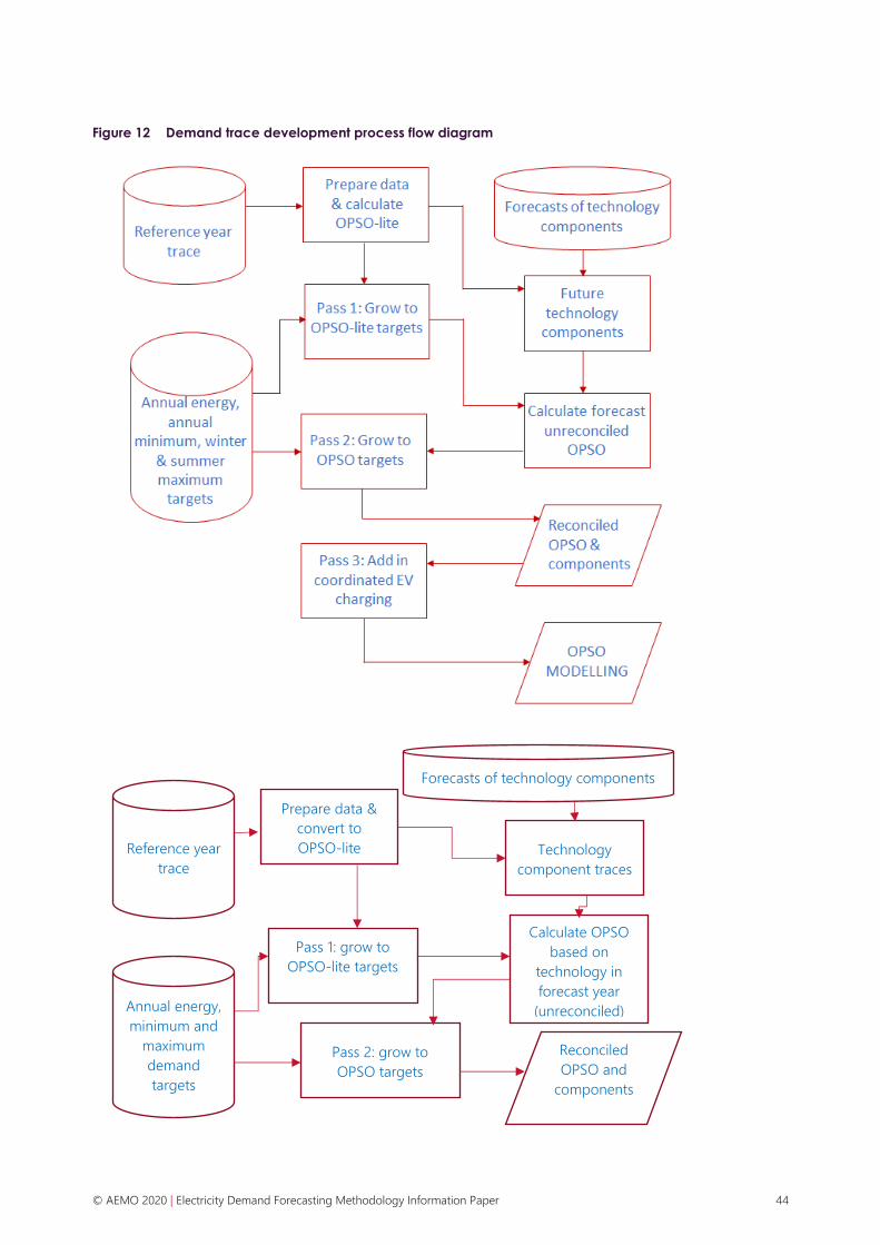
© AEMO 2020 | Electricity Demand Forecasting Methodology Information Paper 44
Figure 12 Demand trace development process flow diagram
Reference year
trace
Annual energy,
minimum and
maximum
demand
targets
Pass 1: grow to
OPSO-lite targets
Prepare data &
convert to
OPSO-lite Technology
component traces
Calculate OPSO
based on
technology in
forecast year
(unreconciled)
Pass 2: grow to
OPSO targets
Reconciled
OPSO and
components
Forecasts of technology components

© AEMO 2020 | Electricity Demand Forecasting Methodology Information Paper 45
6.1 Growth (scaling) algorithm
Demand from the particular reference year was scaled to match the targets of the forecast year using a
constrained optimisation algorithm. The first two passes of the three-pass approach followed this growth
algorithm. The algorithm found scaling factors for each half-hour which minimised the difference between
the adjusted demand and the targets, such that seasonality, weekly and intra-day demand patterns are
preserved. The demand trace was adjusted for each period so that the target was met for each pass. The
approach:
1. Applied a day-swapping algorithm, such that weekends or public holidays in the reference year align with
weekdays or public holidays in the forecast year.
2. Categorised each day in the reference year into day-type groups:
– High-demand days in summer to target the summer maximum demand target.
– High-demand days in winter to target the winter maximum demand target.
– Low-demand half-hour periods to target the annual minimum demand target.
– Other which is used to target the annual consumption target.
A threshold number of days or periods in each group was nominated as an input parameter.
3. Scaled the half-hourly demands across all summer high-demand days such that only the highest demand
point exactly matched the summer maximum demand target.
4. Scaled the half-hourly demands across all winter high-demand days such that only the highest demand
point exactly matched the winter maximum demand target.
5. Scaled the minimum demand across all low-demand half-hour periods such that only the minimum
demand point exactly matched the annual minimum demand target.
6. Determined the scaling factor for each day-type group such that the energy across the year matched the
annual energy target.
7. Calculated future annual energy for each day-type group by multiplying the energy in each day-type
group with demand scaling factors.
8. The “other” day type had no scaling factor for the purpose of meeting a demand target. As such, the
algorithm allocated the remainder of future energy to the ‘other’ day-type category for the purpose of
meeting the annual energy target.
9. Checked the grown traces against the targets. If all targets were met, the process was complete. If any of
the targets were not fully met, the algorithm re-grew the demand traces for the reference year recursively
by repeating steps 1 to 8 until the targets were met. At each repeat the threshold number of days or
periods is increased to enlarge the coverage of periods at which the changes in energy are guided by the
target maxima and minimum.
In the case of negative operational demand, the process managed the handling of periods near or below
zero by adding a fixed amount to all periods before growing. This was then removed after growing.
6.2 Pass 1 – growing to OPSO-lite targets
As highlighted in Figure 12, the first pass grew the OPSO-lite reference year traces to the forecast year
OPSO-lite targets. OPSO-lite is operational demand that has been cleaned to remove atypical demand events
and has had the impact of the following technologies removed:
• Rooftop PV (PVROOF).
• Non-scheduled PV (PVNSG).
• Energy storage systems (ESS).

© AEMO 2020 | Electricity Demand Forecasting Methodology Information Paper 46
• Electric vehicles (EV).
• In the case of Queensland, CSG.
After growing the traces, the technology components were reinstated. This produced an unreconciled OPSO.
The technology components were also prepared to reflect changing installed capacities, vehicle numbers,
installation numbers or, in the case of CSG, demand, such that these components were consistent with the
forecasts for the forecast year.
6.3 Pass 2 – reconciling to the OPSO targets
The second pass sought to ensure that the grown maximum operational demand met the OPSO targets.
Generally, because the trace is based on historical information, the unreconciled OPSO maximum demand
doesn’t always meet the OPSO target once rooftop PV, PVNSG, ESS, EV and CSG were taken into account, as
well as DSP. This is because the OPSO targets were based on simulating weather, while the reference year is a
single weather year. Further, the reference year may be an unexceptional demand year grown to a 10% POE
demand year and this stretching can cause the OPSO targets to be missed.
The second pass re-ran the growth algorithm in Section 5.2 to ensure the OPSO characteristics were met. The
technology components were not modified, therefore this process, in effect, ensured that OPSO targets were
met but could only be done if proximity to OPSO-lite targets was relaxed.
6.4 Pass 3 – adding coordinated EV charging to OPSO
The third phase adds coordinated EV charging to OPSO.
For each day in the demand trace, a daily amount of coordinated EV charging energy is added to the daily
OPSO profile such that the coordinated EV charging fills up the daily half-hourly OPSO troughs. The result is
OPSO-modelling. The approach for each day:
1. Orders the OPSO power profile from lowest to highest.
2. Calculates the corresponding accumulated OPSO energy.
3. Calculates the minimum OPSO power level such that this value adds the necessary energy to OPSO to
match the daily coordinated EV charging energy amount.
4. The new OPSO-modelling power profile is the maximum of the minimum OPSO power level (calculated
from the previous step) and the original OPSO power profile.
5. A stochastic component is added to the OPSO-modelling power profile.
6. Reorders the OPSO-modelling power profile according to time.
6.5 Reporting
AEMO prepared the traces with all the components such that they were modular, and the user could apply
the components to calculate the desired demand definition. The choice of trace definition depended on the
purpose of the modelling performed. For example, the market modelling strategy could elect to model PV
separately or model ESS as a virtual power plant, in turn necessitating control over how those resources were
discharged.

© AEMO 2020 | Electricity Demand Forecasting Methodology Information Paper 47
A1. Electricity retail pricing
AEMO assesses behavioural and structural changes of consumers in response to real or perceived high retail
prices. AEMO calculated the retail price forecasts sourcing a combination of AEMO internal modelling and
publicly available information. Separate prices have been prepared for three market segments:
1. Residential prices.
2. Commercial prices.
3. Industrial prices.
The electricity retail price projections were formed from bottom-up projections based on separate forecasts
of the various components of retail prices:
• Network costs.
• Wholesale costs.
• Environmental costs.
• Retail costs and margins.
The retail price structure followed the Australian Energy Market Commission (AEMC) 2019 Residential
Electricity Price Trends44 report. The wholesale price forecasts are based on AEMO’s Draft 2020 Integrated
System Plan (ISP). Network, environmental and retail components are based on the AEMC‘s report.
Additional transmission development costs associated with AEMO’s ISP central development plan also impact
the total cost. The process of residential pricing modelling is summarised in Table 11.
Commercial and industrial pricing models were developed using the residential pricing model as a baseline.
Each component is then adjusted based on methodology from Jacob’s 2017 Retail Electricity Price History and
Projected Trends Jacobs Report45 and updated using Bloomberg NEF 2019 Australia Behind the Meter
Forecast. Price elasticity coefficients are applied in each of the residential, commercial and industrial models,
details of which are discussed in the respective chapters for these segments.
44 AEMC, 2018 Residential Electricity Price Trends, at https://www.aemc.gov.au/market-reviews-advice/residential-electricity-price-trends-2018.
45 Jacobs, Retail Electricity Price History and Projections, at https://www.aemo.com.au/-/media/Files/Electricity/NEM/Planning_and_Forecasting/Demand-
Forecasts/EFI/Jacobs-Retail-electricity-price-history-and-projections_Final-Public-Report-June-2017.pdf.

© AEMO 2020 | Electricity Demand Forecasting Methodology Information Paper 48
Table 11 Residential pricing model component summary
Component Process summary
Wholesale costs* Wholesale price forecasts based on AEMO’s Draft 2020 Integrated System Plan.
Network costs Use 2019 Residential Electricity Price Trends AEMC Report.
Extrapolate the trajectories based on AEMO’s 2019 ISP Central Optimal Development Path Scenario.
Benchmark against published network tariffs
Environmental costs Use 2019 Residential Electricity Price Trends AEMC Report.
Extrapolate the trajectories based on publicly available information of environmental schemes. These
include federal and state-based renewable energy, energy efficiency and feed-in-tariff schemes.
Retail costs and margin Use 2019 Residential Electricity Price Trends AEMC Report for the base year (FYE 2019) and hold
constant across the forecast period.
* The wholesale costs component of retail price consists of wholesale price, hedging cost, and market charges.

© AEMO 2020 | Electricity Demand Forecasting Methodology Information Paper 49
A2. Weather and climate
A2.1 Heating Degree Days (HDD) and Cooling Degree Days (CDD)
HDD and CDD are measures of heating and cooling demand, respectively. They are estimated by differencing
air temperature from a critical temperature46.
Table 12 Critical regional temperatures for HDD and CDD
Region Critical temperature in degrees C
HDD critical temperature CDD critical temperature
New South Wales 17.0 19.5
Queensland 17.0 20.0
South Australia 16.5 19.0
Tasmania 16.0 20.0
Victoria 16.5 18.0
Note: The HDD and CDD critical temperatures for each region are not BoM standard values but are selected for each region based on
the temperature at which a demand response is detected that demonstrates the greatest predictive power of the models.
The formula for HDD47 is:
𝐻𝐷𝐷 = 𝑀𝑎𝑥(0, CT − �̅�)
The formula for CDD48 is:
𝐶𝐷𝐷 = 𝑀𝑎𝑥(0, �̅� − CT)
Where �̅� is average 30-minute temperature between 9:00 PM of the previous day’s consumption to 9:00 PM
of the consumption day-of-interest, to account for the demand response with temperature that could be due
(in-part) to the previous day’s heat/cool conditions. CT is the critical temperature threshold and is specific to
the region.
HDD and CDD are used in modelling and forecasting of consumption and are calculated at the regional level.
The weather station temperature data is sourced from the BoM49 and the stations used are given below.
46 Critical temperature is a threshold temperature for electricity heating.
47 All the HDDs in a year are aggregated to obtain the annual HDD.
48 All the CDDs in a year are aggregated to obtain the annual CDD.
49 BoM Climate Data, http://www.bom.gov.au/climate/data/.

© AEMO 2020 | Electricity Demand Forecasting Methodology Information Paper 50
Table 13 Weather stations used for HDD and CDD
Region Station name Data range
New South Wales BANKSTOWN AIRPORT AWS 1989/01 ~ Now
Queensland ARCHERFIELD AIRPORT 1994/07 ~ Now
South Australia ADELAIDE (KENT TOWN)* 1993/10 ~ Now
Tasmania HOBART (ELLERSLIE ROAD) 1882/01 ~ Now
Victoria MELBOURNE (OLYMPIC PARK) 2013/05 ~ Now
Victoria MELBOURNE REGIONAL OFFICE 1997/10 ~ 2015/01
* Kent Town station is anticipated to close permanently. Adelaide Airport weather station will be used for South Australia once Kent Town
is unavailable.
A2.2 Determining HDD and CDD standards
The data used to derive a median weather trend are from 2000 to the reference year. AEMO has used the
derived median weather standard for future HDD/CDD projections using a probabilistic methodology for a
given region. This was calculated based on the following formulas:
AnnualHDD = POE50(∑ 𝐻𝐷𝐷 365)
AnnualCDD = POE50(∑ 𝐶𝐷𝐷 365)
where HDD365 is heating degree days over a 365-day period, based on a daily-rolling period starting from
1 January 2000 until the latest available data point in the reference year, and POE50 is where 50% Probability
of Exceedance is expected for the given total heating/cooling degree days within that 365-day period.
Dry-bulb temperature (DBT) is the temperature measured by a thermometer freely exposed to air but
shielded from radiation and moisture. DBT is equivalent to air temperature. In contrast, wet-bulb temperature
(WBT) is the temperature read by a wet-bulb thermometer (a thermometer shrouded in a water-soaked cloth)
over which air is passed. At 100% relative humidity, the wet-bulb temperature is equal to the air temperature
(dry-bulb temperature) and is lower at lower humidity.
A2.3 Climate change
AEMO incorporated climate change into its minimum and maximum demand forecast as well as its annual
consumption forecast. For the annual consumption forecast, average annual temperatures are increasing by a
constant rate. However, half-hourly temperatures have higher variability and increasing extremes due to the
higher frequency of the data.
AEMO collaborated with the BoM and CSIRO to develop a climate change methodology for the purpose of
half-hourly demand forecasting. This process recognised that climate change is impacting temperature
differently across the temperature distribution. Generally, higher temperatures are increasing by more than
average temperatures which are increasing more than low temperatures. This results in higher extreme
temperatures relevant to maximum demand.
The methodology adopted a quantile-to-quantile marching algorithm to statistically downscale publicly
available daily minimum, mean and maximum temperature projects out to 20 to 50 years.
The methodology can be broken into six steps:
• Step 1. Collect climate projection data from www.climatechangeinaustralia.gov.au for weather stations
relevant to the region.

© AEMO 2020 | Electricity Demand Forecasting Methodology Information Paper 51
• Step 2. Collect historical actual half-hourly weather station observations from the BoM and calculate the
daily minimum, mean and maximum temperature.
• Step 3. Calculate the empirical temperature cumulative density function (CDF) in the projection period for
the daily minimum, mean and maximum temperatures.
• Step 4. Calculate the empirical temperature CDF of the historical weather data for the daily minimum,
median and maximum temperatures.
• Step 5. Match the temperature quantiles of the projected temperature distribution with the quantiles of
the historical temperature distribution. Assign a scaling factor for each quantile for daily minimum,
mean/median and maximum temperature to transform the historical temperatures to the distribution of
projected temperatures.
• Step 6. Interpolate the daily minimum, mean/median and maximum scaling factor for each quantile down
to the half-hourly level.
Step 1 – Collect daily temperature projection data
• Collect daily minimum and maximum temperature projection data from
https://www.climatechangeinaustralia.gov.au/en/climate-projections/explore-data/data-download/station-
data-download/.
• Collect data for each climate model:
– ACCESS1-0, CanESM2, CESM1-CAM5, CNRM-CM5, GFDL-ESM2M, HadGEM2, MIROC5, NorESM1
• The mean temperature for each day is calculated (i.e., simple average equated as (daily minimum + daily
maximum)/2).
Step 2 – Collect historical actual half-hourly temperature observations and calculate daily
minimum, median and maximum
• Collect half-hourly temperature data for weather stations in each region relevant to the energy demand
centres of those regions.
• Find the daily minimum, median and maximum temperatures.
• To ensure that the daily mid-point matches to an actual half-hourly value the median is used in place of
the daily mean. As temperature is (normally) normally distributed the median should be roughly equal to
the mean to within a fraction of a percent.
Step 3 – Calculate the empirical temperature CDF of projected daily temperatures data
• Set up an 11-year rolling window to account for variability in weather between different years including the
eight different weather models in the same window (in effect 8 * 11 years in the window).
• Rank the daily minimum, mean and maximum temperatures from lowest to highest for the 11-year window
including the eight weather models.
• Attribute a percentile to each temperature value in the forecast horizon.
Step 4 – Calculate the empirical temperature CDF of historical daily observations
• Set up an 11-year rolling window to account for variability in weather between different years.
• Rank the daily minimum, median and maximum temperatures from lowest to highest for the 11-year
window.
• Attribute a percentile to each temperature value in history.

© AEMO 2020 | Electricity Demand Forecasting Methodology Information Paper 52
Step 5 – Map historical temperature quantiles to projected temperature quantiles and assign a
scaling factor
• Map quantiles of the forecast model daily CDF onto quantiles of the historical CDF.
• Calculate a scaling factor for each quantile for daily minimum, mean/median and maximum temperatures.
Step 6 – Interpolate daily scaling factors to half-hourly and scale
• Rank the 48 half-hourly temperature observations for each day from the daily minimum to the daily
midpoint and to the daily maximum.
• Interpolate the scaling factor for each half-hour.
• Scale up each historical half-hour for each historical weather year to match each projected weather years.
The final result is a table with dimensions 𝑇𝐴 × 𝑇𝐻 × 17520, where:
• 𝑇ℎ is the number of historical actual weather years.
• 𝑇𝐻 is the number of projected weather years in the forecast horizon.
• 17520 half-hourly data points in each weather year.

© AEMO 2020 | Electricity Demand Forecasting Methodology Information Paper 53
A3. Rooftop PV and energy storage
A3.1 Rooftop PV forecast
A3.1.1 Installed capacity forecast
AEMO’s 2020 forecast of installed capacity for rooftop PV (installations with a capacity < 100 kW) was based
on advice from two external consultants, Green Energy Markets (GEM) and CSIRO.
Table 14 below provides details on the scenario mapping used for the 2020 ESOO scenarios; the forecast
methodologies are available in CSIRO’s and GEM’s published reports50,51. This scenario mapping was
developed after consultation with stakeholders in the March 2020 Forecasting Reference Group (FRG)52
meeting and considers the relationship between the PV and battery forecasts to capture a broad range of
scenario possibilities.
Table 14 Mapping of consultant trajectories used for DER forecasts
ESOO scenarios ISP scenarios
Slow Change Central Step Change Fast Change High DER
PV CSIRO Slow Change
Average of CSIRO
Central and GEM
Central
GEM Step Change
Average of CSIRO
Fast Change and
GEM Fast Change
GEM High DER
Embedded
battery
systems CSIRO Slow Change
Average of CSIRO
Central and GEM
Central
GEM Step Change
Average of CSIRO
Fast Change and
GEM Fast Change
GEM High DER
Electric
Vehicles CSIRO Slow Change CSIRO Central CSIRO Step Change
CSIRO Fast Change CSIRO High DER
The main drivers behind the forecast rooftop PV uptake are:
• Financial incentives, such as Small Technology Certificates (STCs) and feed-in tariffs (FiTs).
• Installation costs, including both system/component costs and non-hardware “soft costs”, including
marketing and customer acquisition, system design, installation labour, permitting and inspection costs,
and installer margins.
50 CSIRO, 2020 projections for small-scale embedded technologies report, at https://aemo.com.au/-/media/files/electricity/nem/planning_and_forecasting/
inputs-assumptions-methodologies/2020/csiro-der-forecast-report.pdf?la=en.
51 GEM, 2020 Projections for distributed energy resources – solar PV and stationary energy battery systems report, at https://aemo.com.au/-
/media/files/electricity/nem/planning_and_forecasting/inputs-assumptions-methodologies/2020/green-energy-markets-der-forecast-report.pdf?la=en
52 For FRG minutes and presentation see https://aemo.com.au/en/consultations/industry-forums-and-working-groups/list-of-industry-forums-and-working-
groups/forecasting-reference-group-frg#:~:text=The%20Forecasting%20Reference%20Group%20(FRG,AEMO%20and%20industry's%20forecasting%20
specialists.&text=It%20is%20an%20opportunity%20to,not%20a%20decision%20making%20body.
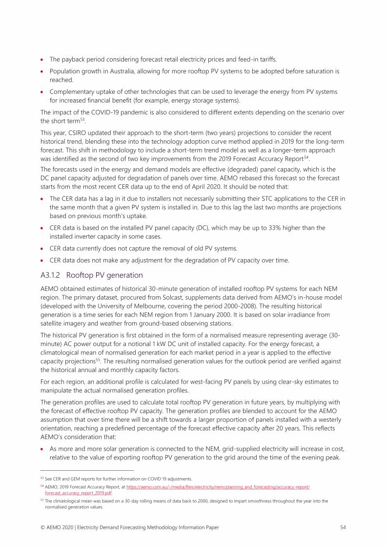
© AEMO 2020 | Electricity Demand Forecasting Methodology Information Paper 54
• The payback period considering forecast retail electricity prices and feed-in tariffs.
• Population growth in Australia, allowing for more rooftop PV systems to be adopted before saturation is
reached.
• Complementary uptake of other technologies that can be used to leverage the energy from PV systems
for increased financial benefit (for example, energy storage systems).
The impact of the COVID-19 pandemic is also considered to different extents depending on the scenario over
the short term53.
This year, CSIRO updated their approach to the short-term (two years) projections to consider the recent
historical trend, blending these into the technology adoption curve method applied in 2019 for the long-term
forecast. This shift in methodology to include a short-term trend model as well as a longer-term approach
was identified as the second of two key improvements from the 2019 Forecast Accuracy Report54.
The forecasts used in the energy and demand models are effective (degraded) panel capacity, which is the
DC panel capacity adjusted for degradation of panels over time. AEMO rebased this forecast so the forecast
starts from the most recent CER data up to the end of April 2020. It should be noted that:
• The CER data has a lag in it due to installers not necessarily submitting their STC applications to the CER in
the same month that a given PV system is installed in. Due to this lag the last two months are projections
based on previous month’s uptake.
• CER data is based on the installed PV panel capacity (DC), which may be up to 33% higher than the
installed inverter capacity in some cases.
• CER data currently does not capture the removal of old PV systems.
• CER data does not make any adjustment for the degradation of PV capacity over time.
A3.1.2 Rooftop PV generation
AEMO obtained estimates of historical 30-minute generation of installed rooftop PV systems for each NEM
region. The primary dataset, procured from Solcast, supplements data derived from AEMO’s in-house model
(developed with the University of Melbourne, covering the period 2000-2008). The resulting historical
generation is a time series for each NEM region from 1 January 2000. It is based on solar irradiance from
satellite imagery and weather from ground-based observing stations.
The historical PV generation is first obtained in the form of a normalised measure representing average (30-
minute) AC power output for a notional 1 kW DC unit of installed capacity. For the energy forecast, a
climatological mean of normalised generation for each market period in a year is applied to the effective
capacity projections55. The resulting normalised generation values for the outlook period are verified against
the historical annual and monthly capacity factors.
For each region, an additional profile is calculated for west-facing PV panels by using clear-sky estimates to
manipulate the actual normalised generation profiles.
The generation profiles are used to calculate total rooftop PV generation in future years, by multiplying with
the forecast of effective rooftop PV capacity. The generation profiles are blended to account for the AEMO
assumption that over time there will be a shift towards a larger proportion of panels installed with a westerly
orientation, reaching a predefined percentage of the forecast effective capacity after 20 years. This reflects
AEMO’s consideration that:
• As more and more solar generation is connected to the NEM, grid-supplied electricity will increase in cost,
relative to the value of exporting rooftop PV generation to the grid around the time of the evening peak.
53 See CER and GEM reports for further information on COVID 19 adjustments.
54 AEMO, 2019 Forecast Accuracy Report, at https://aemo.com.au/-/media/files/electricity/nem/planning_and_forecasting/accuracy-report/
forecast_accuracy_report_2019.pdf.
55 The climatological mean was based on a 30-day rolling means of data back to 2000, designed to impart smoothness throughout the year into the
normalised generation values.
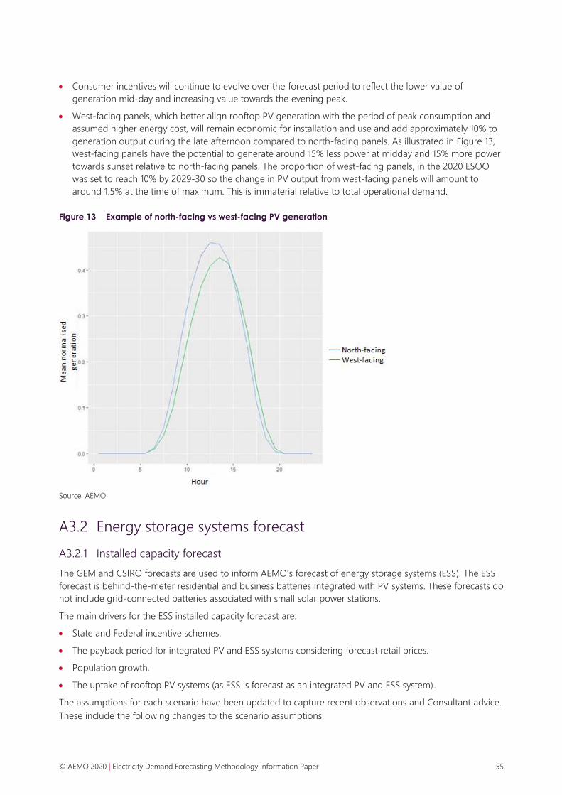
© AEMO 2020 | Electricity Demand Forecasting Methodology Information Paper 55
• Consumer incentives will continue to evolve over the forecast period to reflect the lower value of
generation mid-day and increasing value towards the evening peak.
• West-facing panels, which better align rooftop PV generation with the period of peak consumption and
assumed higher energy cost, will remain economic for installation and use and add approximately 10% to
generation output during the late afternoon compared to north-facing panels. As illustrated in Figure 13,
west-facing panels have the potential to generate around 15% less power at midday and 15% more power
towards sunset relative to north-facing panels. The proportion of west-facing panels, in the 2020 ESOO
was set to reach 10% by 2029-30 so the change in PV output from west-facing panels will amount to
around 1.5% at the time of maximum. This is immaterial relative to total operational demand.
Figure 13 Example of north-facing vs west-facing PV generation
Source: AEMO
A3.2 Energy storage systems forecast
A3.2.1 Installed capacity forecast
The GEM and CSIRO forecasts are used to inform AEMO’s forecast of energy storage systems (ESS). The ESS
forecast is behind-the-meter residential and business batteries integrated with PV systems. These forecasts do
not include grid-connected batteries associated with small solar power stations.
The main drivers for the ESS installed capacity forecast are:
• State and Federal incentive schemes.
• The payback period for integrated PV and ESS systems considering forecast retail prices.
• Population growth.
• The uptake of rooftop PV systems (as ESS is forecast as an integrated PV and ESS system).
The assumptions for each scenario have been updated to capture recent observations and Consultant advice.
These include the following changes to the scenario assumptions:

© AEMO 2020 | Electricity Demand Forecasting Methodology Information Paper 56
• The FYE 2019 estimated actual data has been revised upwards by 55 MW, based on updated battery
estimated actuals information56.
• The degradation adjustment has been removed from battery MW and is only applied to MWh in line with
industry advice received by the consultants.
• Updated population and economic forecasts.
• Development of state specific representative customer load profiles57, which are linked to the 19 years of
estimated historic rooftop PV generation by state described in A3.1.
• Updates to the battery and balance of plant installed costs based on Draft GenCost 2019-2058 forecasts.
• Revised retail tariff assumptions, with a smaller proportion of customers accessing smart tariffs in the
Central scenario based on low historical consumer interest in opt-in time-of-use tariffs.
• Updated CSIRO forecast approach, using the recent historical trend to inform the short term forecast
before blending into the technology adoption curve approach used in 2019.
• A revised scenario mapping approach, combining both GEM and CSIRO battery forecasts as detailed in
Table 14.
A3.2.2 ESS charge discharge profile used in minimum and maximum demand
CSIRO also provided AEMO the daily charge and discharge profile for behind-the-meter ESS used in the
minimum and maximum demand modelling. The profiles were based on historical solar irradiance (as ESS is
assumed to primarily charge from excess rooftop PV generation) and with the strategy to minimise
household/commercial business bills without any concern for whether the aggregate outcome is also
optimised for the electricity system.
The demand forecasts consider two types of battery operation:
• Shift Solar, where the battery will charge when excess solar PV generation is available and discharge
whenever solar PV generation is insufficient to cover household demand
• Time of Use tariff (TOU), where the battery is optimised to take advantage of a time of use tariff, top up
charge at off peak times to maximise avoidance of peak time tariffs.
A third operating type, control of battery by an aggregator, commonly referred to as a virtual power plant
(VPP), with the battery operation optimised to reduce overall system costs and operated as a scheduled,
controllable form of generation, much like a traditional form of grid-generated electricity supply.
The proportions of each battery operating type are provided in Table 15 below.
Table 15 New South Wales Central scenario tariff and associated battery operating type shares
Customer Class Shift solar TOU Virtual Power Plant (VPP)
2030 2050 2030 2050 2030 2050
Residential 76% 68% 6% 2% 18% 30%
Commercial 14% 12% 56% 48% 30% 40%
56 Average battery size information was sourced from market intelligence provided by a third party consultant to CSIRO (SunWiz).
57 See Appendix A.2 of Projections for small-scale embedded technologies, 2019.
58 Graham, Paul; Hayward, Jenny; Foster, James; Havas, Lisa. GenCost 2019-20. CSIRO publications repository: CSIRO; 2020, at
https://doi.org/10.25919/5eb5ac371d372.

© AEMO 2020 | Electricity Demand Forecasting Methodology Information Paper 57
To calculate the effect of batteries contribution to the 2020 ESOO demand profile forecasts, CSIRO developed
a detailed set of normalised battery charge/discharge profiles. These profiles were developed using New
South Wales customer load profile data for from the Smart Grid Smart Cities program run by Ausgrid. CSIRO
provided load profiles for each region based from these profiles, with regions other than NSW adjusted
based on zone substation data.
Figure 14 compares the charge/discharge profiles of the two battery operating types for New South Wales for
February . Actual charge/discharge profile will depend on a range of factors including the actual availability of
solar resources to charge the battery system, household consumption, and battery size.
Figure 14 New South Wales average daily February profile
The charge/discharge profiles have the effect of smoothing out demand across the day and reducing
maximum demand, however for shift solar and shift peak battery operating types, the effect per battery at
reducing the operational demand at peak times in summer is relatively small given that battery operations are
targeting residential load reductions, rather than whole-of-grid reductions.
A3.2.3 ESS in annual consumption
ESS stores energy for later use, but in so doing incurs electrical losses as indicated by a battery’s round-trip
efficiency. In the 2020 forecasts, the round-trip efficiency is assumed to be 85%. That is, for each 1 kWh of
energy stored in the battery, 15% of that energy is lost in the process of charging and then discharging the
battery. This lost energy is accounted for in business and residential consumption forecasts as an additional
form of energy consumption applying the expected level of battery operation. These losses are small relative
to NEM operational consumption, accounting for <0.01 % of total electricity consumption by 2038-39 in the
Central scenario.

© AEMO 2020 | Electricity Demand Forecasting Methodology Information Paper 58
A4. Electric vehicles
A4.1.1 Electric vehicles forecast
CSIRO developed AEMO’s forecast of EVs, including residential, light commercial, and heavy commercial
vehicles such as buses and trucks. The most recent CSIRO report is available on AEMO’s website59.
The main drivers for the EV forecast are:
• Relative price between EV and alternatives.
• Payback period – EVs have higher upfront costs in the initial period of the forecast but lower “fuel” cost as
kW per km.
• Level of increased ride sharing – reducing the number of vehicles.
• Battery and technology improvements.
• Limiting factors such as renter’s access to external household charging points.
• Full decarbonisation of transport by 2050 (considered in Step Change scenario only).
A4.1.2 Electric vehicles charge profiles used in minimum and maximum demand
Consultancies also provided AEMO the daily charge and discharge profile for EVs used in the minimum and
maximum demand modelling.
Four different charge profiles are applied in the 2020 forecasts:
• Convenience charging – vehicles assumed to have no incentive to charge at specific times, resulting in
greater evening charging after vehicles return to the garage.
• Daytime charging – vehicles incentivised to take advantage of high PV generation during the day, with
available associated infrastructure to enable charging at this time. For 2020 this was further split so that a
proportion of day time charging EV was assumed to be managed by a VPP or charging aggregator to
minimise peak demand events driven by EV charging (See Table 16).
• Night-time charging – vehicles incentivised to take advantage of low night-time demand. For 2020 this
was further split so that a proportion of night time charging EV was assumed to be managed by a VPP or
charging aggregator to minimise peak demand events driven by EV charging (See 0). Highway fast
charging – vehicles that require a fast charging service while in transit, based on a mix of simulated and
actual arrivals of vehicles at public fast charging from CSIRO research.
The charge profiles are used in the minimum and maximum demand simulation process and load trace
growing algorithm.
59 At https://www.aemo.com.au/Electricity/National-Electricity-Market-NEM/Planning-and-forecasting/Inputs-Assumptions-and-Methodologies.

© AEMO 2020 | Electricity Demand Forecasting Methodology Information Paper 59
Table 16 Assumed proportion of daytime charging that is managed, by scenario
FYE Central Fast Change High DER Slow Change Step Change
2030 0% 0% 0% 0% 0%
2040 40% 40% 50% 0% 50%
2050 80% 80% 100% 0% 100%
Table 17 Assumed proportion of night-time charging that is managed, by scenario
FYE Central Fast Change High DER Slow Change Step Change
2030 0% 0% 0% 0% 0%
2040 30% 30% 50% 0% 50%
2050 60% 60% 100% 0% 100%
A4.1.3 Electric vehicles annual consumption
For the purpose of annual consumption, EVs travel a certain number of kilometres in a year, with a certain
level of efficiency per charge. The time of charge is not important when considering annual consumption.

© AEMO 2020 | Electricity Demand Forecasting Methodology Information Paper 60
A5. Connections and uptake of electric appliances
A5.1 Connections
As the retail market operator for most Australian electricity retail markets (except the Northern Territory and
Tasmania), AEMO has access to historical connections data for these markets; historical connections data for
the other markets are acquired from a confidential survey. AEMO forecasts the number of new connections to
the electricity network, starting from the most recent data history, as this is a key driver for residential
electricity demand. The number of new connections is driven by demographic and social factors like
household projections, which is determined by population projections and changes to household density.
The electricity connection forecasts were made up of two components, residential and non-residential
electricity connection forecasts. AEMO only used the residential electricity connections to forecast residential
sector consumption. The non-residential component was captured by the commercial sector which is driven
by economic indicators. Therefore, AEMO underwent a process of splitting the residential connections
projections from the non-residential connections60.
For the 2020 ESOO, AEMO engaged Conach to develop a residential building stock model that forms the
basis of the connections forecast. The building stock model takes actual household numbers from the
Australian Bureau of Statistics (ABS) 2016 census and grows the household numbers from 2017 to 2019 using
the NMI connections growth rate, due to both the updated data for connections since the ABS census and
the stable growth rate making the use of a trend variable appropriate.
From 2020 to 2023, the building stock model transitions from using the NMI connections growth rate to the
ABS household projections (Cat. No. 3236.0) on a sliding scale of 0% to 100%. The ABS Household Projections
data provides three series – Series 1 (upper), Series II (middle) and Series III (lower) – that have been applied
to the Step Change, Central and Slow Change scenarios. From 2024 onwards, the building stock model
applies only the ABS Household Projections. AEMO used recent data on connections per household to
convert the building stock model for each scenario into connections forecasts. Further spread between the
scenarios is drawn from construction sector activity (Division E) per capita relative to the Central scenario,
based on the economic consultants economic and population forecasts.
It is anticipated that COVID-19 will reduce the demand for new building construction, and AEMO has adjusted
the connections forecast based on published housing industry reports61.
60 Residential connections forecasts are available on AEMO’s Forecasting Data Portal, at http://forecasting.aemo.com.au.
61 See https://hia.com.au/-/media/HIA-Website/Files/Media-Centre/Media-Releases/2020/national/half-a-million-jobs-at-risk.ashx.

© AEMO 2020 | Electricity Demand Forecasting Methodology Information Paper 61
A5.2 Uptake and use of electric appliances
AEMO uses appliance data from the former Australian Government Department of the Environment and
Energy62 to forecast growth in electricity consumption by the residential sector.
The data allowed AEMO to estimate changes to the level of energy services supplied by electricity per
households across the NEM. Energy services here is a measure based on the number of appliances per
category across the NEM, their usage hours, and their capacity and size. Figure 15 illustrates the difference
between energy services and energy consumption.
Figure 15 Energy services vs energy consumption
A5.2.1 Appliance growth calculation
The following lists how AEMO calculates energy services by appliance group.
• Heating/cooling: Number of appliances × output capacity of appliance × hours used per year.
• White goods: Number of appliances × capacity (volume of freezer/refrigerators/washing machine) ×
number of times used per year (dishwashers, washing machines and dryers only).
• Home entertainment: Number of appliances × hours used per year × size (TVs only).
• Lighting: Number of light fittings.
• Cooking: Number of appliances x hours used per year.
• Hot water: Number of appliances x hours used per year.
62 AEMO would like to thank the E3 Committee for access to the appliance model underpinning the 2015 Residential Baseline Study for Australia 2000 – 2030,
(RBS, 2015) available at www.energyrating.com.au.

© AEMO 2020 | Electricity Demand Forecasting Methodology Information Paper 62
The calculated demand for energy services by appliance group is converted into a growth index for each load
type, with the reference year of the consumption forecast being the base year (index = 100). For baseload, the
relevant appliance groups are combined into a composite index based on their relative estimate energy
consumption in the base year. AEMO divides the appliance growth indices by the number of households63 in
a forecast year.
The table below shows the appliances covered by the calculations.
Table 18 List of appliance categories used in calculating the appliance growth index
Load type Category Group
Heating/cooling load Combined space heating/cooling AC ducted
AC non-ducted (split and window/wall units)
Heating/cooling load Space cooling Evaporative (mostly central)
Fans
Heating/cooling load Space heating Electric resistive
Mains gas non-ducted
Mains gas ducted
LPG gas non-ducted
Wood Heaters
Base load White goods Refrigerators
Freezers
Dishwashers
Clothes washers
Clothes dryers
Base load IT & Home Entertainment Television – composite average
Set-top box – free-to-air
Set-top box – subscription
Video players and media recorders
Home entertainment – other (mostly audio)
Game consoles
Computers – desktop (and associated monitors)
Computers – laptop
Wireless/Wired networking device
Miscellaneous IT equipment
Base load Lighting MV incandescent
MV halogen
ELV halogen
CFL
Linear fluorescent
LED
Base load Cooking Products Upright – Electric
Cooktop – Electric
63 AEMO uses household data from RBS 2015 for consistency

© AEMO 2020 | Electricity Demand Forecasting Methodology Information Paper 63
Load type Category Group
Oven – Electric
Upright – Gas
Cooktop – Gas
Oven – Gas
Upright – LPG
Cooktop – LPG
Oven – LPG
Microwave
Base load Hot water heaters Electric water heater, storage – small
Electric water heater, storage – medium/large
Electric water heater, instant
Gas water heater, storage (mains)
Gas water heater, storage (LPG)
Gas water heater, instant (mains)
Gas water heater, instant (LPG)
Solar electric
Solar gas
Heat pump
Wood, wetbacks
Base load Other Equipment Pool Equipment – Electric
Pool Equipment – Gas
Pumps
Battery chargers
Miscellaneous
Class 2 Common Areas
A5.2.2 Difference between scenarios
In addition to forecast changes in appliance uptake and use for known appliance categories, AEMO adds to
the composite index a small increase in growth from “new” appliance types/categories (not shown specifically
in Table 18), representing yet unknown technologies that are expected to enter the market over the forecast
period and affect electricity demand. The three scenarios have different assumptions of how much these new
and yet unknown appliances would add to the composite appliance growth index.
AEMO made further adjustments to the number of appliances in the space heating and hot water heating
categories, to account for policy-induced fuel switching behaviour from gas to electricity. In 2020, the policies
considered were the National Construction Code 2022 for water heating, the Victorian Solar Homes Program
for solar electric water heating, the ACT Gas Heater Rebate, and the planned E3 Zoned Space Heating Label
Program. Adjustments vary by scenario and reflect similar adjustments in the 2020 GSOO fuel switching
model. AEMO also estimated the potential impact of the ACT Government’s Climate Change Strategy, which
is legislated to achieve net zero emissions from gas use by 204564.
64 ACT Government, ACT Climate Change Strategy 2019-2025, at https://www.environment.act.gov.au/__data/assets/pdf_file/0003/1414641/ACTClimate-
Change-Strategy-2019-2025.pdf.

© AEMO 2020 | Electricity Demand Forecasting Methodology Information Paper 64
AEMO provides further dispersion across the scenarios by applying a per capita Household Disposable
Income (HDI) index to the Slow Change and Step Change scenarios, relative to the per capita HDI for the
Central scenario.
A5.2.3 COVID-19 adjustments
AEMO considered the impact of significant restrictions in movement outside of the household and the likely
effect on the appliance growth indices. While the economic downturn reduced household spending,
particularly for displaced workers, a sizeable portion of the workforce rapidly transitioned to work from home
arrangements. This is supported by observations of residential meter data, that indicates a 10 to 15% increase
in consumption for the sector.
AEMO applied a short-term bounce in consumption of approximately half this value in the Step Change,
should six months of this sustain usage remain, with a lower level applied to the Central and Slow Change
scenarios. AEMO assumed a smaller adjustment in the 2022, as mobility is expected to increase towards
pre-COVID levels. In the Central and Step Change scenarios, a modest adjustment is applied in the longer
term to account for some working from home practices persisting. Table 19 lists the COVID adjustments made
to the appliance growth indices.
Table 19 COVID adjustments to the appliance growth indices
Financial year Central Step Change Slow Change
2020-21 3.5% 6% 2%
2021-22 1.0% 2% 0.5%
2022-23 and beyond 0.5% 1% 0%

© AEMO 2020 | Electricity Demand Forecasting Methodology Information Paper 65
A6. Data sources
Table 20 ANZSIC code mapping for industrial sector disaggregation
ANZSIC division ID ANZSIC division name AEMO sector category
A Agriculture, Forestry and Fishing Other
B Mining (including CSG) Other
C Manufacturing Manufacturing
D Electricity, Gas, Water and Waste Services Other
E Construction Other
F Wholesale Trade Other
G Retail Trade Other
H Accommodation and Food Services Other
I Transport, Postal and Warehousing Other
J Information Media and Telecommunications Other
K Financial and Insurance Services Other
L Rental, Hiring and Real Estate Services Other
M Professional, Scientific and Technical Services Other
N Administrative and Support Services Other
O Public Administration and Safety Other
P Education and Training Other
Q Health Care and Social Assistance Other
R Arts and Recreation Services Other
S Other Services Other

© AEMO 2020 | Electricity Demand Forecasting Methodology Information Paper 66
Table 21 Historical and forecast input data sources
Data series Data sources Reference Notes
Historical Consumption
data by region AEMO Database http://forecasting.aemo.com.au/ Actuals derived from
aggregate of these sources
are reported and available
on our forecasting data
portal
Historical Consumption
data by industry sector AEMO Database http://forecasting.aemo.com.au/ Actuals derived from
aggregate of these sources
are reported and available
on our forecasting data
portal
Large Industrial Historical
Consumption data by
region
Transmission & Distribution,
Industrial Surveys
http://forecasting.aemo.com.au/ Actuals derived from
aggregate of these sources
are reported and available
on our forecasting data
portal
Residential and
Commercial Historical
Consumption data by
region
AEMO Database (for
Victoria)
Distribution businesses
(other regions)
http://forecasting.aemo.com.au/ Actuals derived from
aggregate of these sources
are reported and available
on our forecasting data
portal
Weather & Climate Change
Data BOM http://www.bom.gov.au/http:.
Weather & Climate Change
Data CSIRO https://www.csiro.au/
Weather & Climate Change
Data Climate Change Australia https://www.climatechangeinaustral
ia.gov.au/
Historical Number of NMIs AEMO Database http://forecasting.aemo.com.au/ Actuals derived from
aggregate of these sources
are reported and available
on our forecasting data
portal
ABS Household Projections ABS
https://www.abs.gov.au/ausstats/ab
[email protected]/mf/3236.0
AEMO uses household
projections series I (Step
change scenario); series II
(Central scenario); series II
(Slow change scenario)
Demographic and
Economic Data ABS http://www.abs.gov.au/AUSSTATS/a
[email protected]/DetailsPage/5206.0Mar%2
02014?OpenDocument
Population, Gross State
Product, Household
Disposable Income, Input
Producer Price Index,
Economic Data Economic Consultancy (BIS
Oxford Economics)
Original:
https://www.aemo.com.au/-
/media/files/electricity/nem/plannin
g_and_forecasting/inputs-
assumptions-
methodologies/2020/bis-oxford-
economics-macroeconomic-
projections.pdf?la=en
COVID-19 update:
Economic projections were
developed by an economic
consultant, according to
AEMO’s scenario
requirements

© AEMO 2020 | Electricity Demand Forecasting Methodology Information Paper 67
Data series Data sources Reference Notes
https://aemo.com.au/-
/media/files/electricity/nem/plannin
g_and_forecasting/inputs-
assumptions-
methodologies/2020/bis-oxford-
economics-macroeconomic-
central-scenario-and-downside-
scenario-forecast.pdf?la=en
Wholesale Electricity Price AEMO ISP https://www.aemo.com.au/Electricit
y/National-Electricity-Market-
NEM/Planning-and-
forecasting/Integrated-System-Plan
Wholesale price forecasts by
AEMO
DER forecasts CSIRO and GEM https://aemo.com.au/-
/media/Files/Electricity/NEM/Planni
ng_and_Forecasting/Inputs-
Assumptions-
Methodologies/2020/CSIRO-DER-
Forecast-Report
https://aemo.com.au/-
/media/files/electricity/nem/plannin
g_and_forecasting/inputs-
assumptions-
methodologies/2020/green-
energy-markets-der-forecast-
report.pdf?la=en
Transmission losses AEMO database (Victoria);
Transmission businesses
(other regions)
https://www.aemo.com.au/Electricit
y/National-Electricity-Market-
NEM/Security-and-reliability/Loss-
factor-and-regional-boundaries
Distribution losses AEMO database (Victoria);
Distribution businesses
(other regions)
https://www.aemo.com.au/Electricit
y/National-Electricity-Market-
NEM/Security-and-reliability/Loss-
factor-and-regional-boundaries
Auxiliary Factors GHD 2018-19 Costs and
Technical Parameters
https://www.aemo.com.au/-
/media/Files/Electricity/NEM/Planni
ng_and_Forecasting/Inputs-
Assumptions-
Methodologies/2019/GHD-AEMO-
revised---2018-19-
Costs_and_Technical_Parameter.xlsb
Operational demand AEMO database (Victoria),
Transmission businesses
where permission has been
granted
http://forecasting.aemo.com.au/ Actuals derived from
aggregate of these sources
are reported and available
on our forecasting data
portal
Energy data by Industry
Code Department of Environment
and Energy Data Statistics
https://www.energy.gov.au/publicat
ions/australian-energy-update-2019
Table F

© AEMO 2020 | Electricity Demand Forecasting Methodology Information Paper 68
A7. Data segmentation
AEMO used a hybrid model, a combination of two different methods, to calculate the half-hourly Residential
and Business split for the latest year of actual consumption, which forms the starting point for the forecasting
process. As illustrated in Figure 16, this hybrid method utilises the combination of AER Derived Annual
Residential-Business Split (top-down) and Residential Derived Daily Residential-Business Split (bottom-up)
methods to calculate the half-hourly Residential and Business consumptions. Herein the names top-down and
bottom-up to denote the two approaches. This process provides:
• Delivered consumption.
• Underlying consumption.
For the definitions of the consumption types, see Section 1.3.
The bottom up method is used for all NEM regions, except Tasmania which has lower amount of smart
meter connection. As a result, Tasmania is based on the top-down approach.
Figure 16 Hybrid model used to calculate the half-hourly residential and business split
A7.1 AER-derived annual residential-business split: top-down
method
The top-down method used a combination of Residential to Business annual percentage splits (provided to
AEMO by the AER) and its own meter data classification to calculate the half-hourly residential and business
split for the latest year of actual consumption.
A7.1.1 AER residential to business splits
The AER annually surveys distribution network service providers and from this provides AEMO with residential
to business sector annual splits of distribution connected delivered consumption for the latest financial year

© AEMO 2020 | Electricity Demand Forecasting Methodology Information Paper 69
of data available. AEMO used this to derive annual consumption targets to calibrate to when performing half-
hourly splits between residential and business sector consumption. The configuration and execution of the
separate business and residential forecast models – with their different demand drivers – will determine the
total for the business and residential components for each subsequent period in the forecast.
A7.1.2 AEMO meter data and half-hourly profile
Since the introduction of smart metering technology in 2003, there has been varied adoption of smart meters
across states. While all meters in Victoria have been transitioned to smart meters, in other states there are still
many households and smaller businesses on basic meters.
The key distinction is that smart meter reads give actual recording of delivered consumption at the
half-hourly level while basic meters are read quarterly and require some estimation to interpolate into
half-hourly delivered consumption. Typically, most basic meter customers are residential customers while
most businesses have transitioned to smart meters (also known as interval meters).
With this assumption in mind, AEMO preserved the profile of business half-hourly data over a financial year
(as it was deemed more accurate), but determined the profile of the residential half-hourly data by taking the
difference between the total grid consumption half-hourly profile (derived from the metred half hourly
operational demand data) and the business half-hourly profile.
Business half-hourly data
In 2015, AEMO conducted a meter data analytics study to refine the classification of its business meters. While
it is not possible to capture all business sector meters, the bulk of the business delivered consumption was
captured by querying AEMO’s database and then scaling up to meet the target annual business delivered
consumption, derived by applying AER’s business percentage to AEMO’s total delivered annual consumption.
A7.1.3 Methodology
Stage 1: Developing residential to business delivered consumption split
Calculate delivered consumption to energy users from the metered operational demand (as generated) data,
netting off auxiliary load and distribution and transmission losses and adding in the small non-scheduled
generation (PVNSG and ONSG):
Translate AEMO half-hourly meter data into distribution connected delivered consumption:
Transmission-connected consumption was assumed to be business load, and was separated from the total
demand to keep AEMO’s meter data on the same basis as the AER’s percentage splits.

© AEMO 2020 | Electricity Demand Forecasting Methodology Information Paper 70
Aggregate AEMO half-hour data to financial year data and apply AER split to obtain annual target:
Calculate business scaling factor and scale half-hourly business delivered data to annual target:
The unscaled distribution-connected business delivered consumption is the aggregate consumption of the
known business sector meters (for more detail see Business half-hourly data above). This consumption was
summed to the annual level and the total delivered business consumption annual target (derived in the
previous step) was divided by this unscaled business consumption to get a scaling factor. This scaling factor
was applied to the half-hour frequency unscaled business delivered consumption to get the total half-hour
distribution connected delivered business consumption. In this way, AEMO preserves the business sector half
hourly profile and calibrates to an annual target to capture any missing business sector meters.
Calculate business half-hourly delivered consumption:
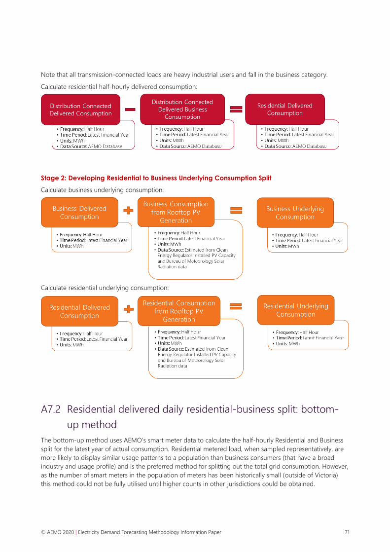
© AEMO 2020 | Electricity Demand Forecasting Methodology Information Paper 71
Note that all transmission-connected loads are heavy industrial users and fall in the business category.
Calculate residential half-hourly delivered consumption:
Stage 2: Developing Residential to Business Underlying Consumption Split
Calculate business underlying consumption:
Calculate residential underlying consumption:
A7.2 Residential delivered daily residential-business split: bottom-
up method
The bottom-up method uses AEMO’s smart meter data to calculate the half-hourly Residential and Business
split for the latest year of actual consumption. Residential metered load, when sampled representatively, are
more likely to display similar usage patterns to a population than business consumers (that have a broad
industry and usage profile) and is the preferred method for splitting out the total grid consumption. However,
as the number of smart meters in the population of meters has been historically small (outside of Victoria)
this method could not be fully utilised until higher counts in other jurisdictions could be obtained.
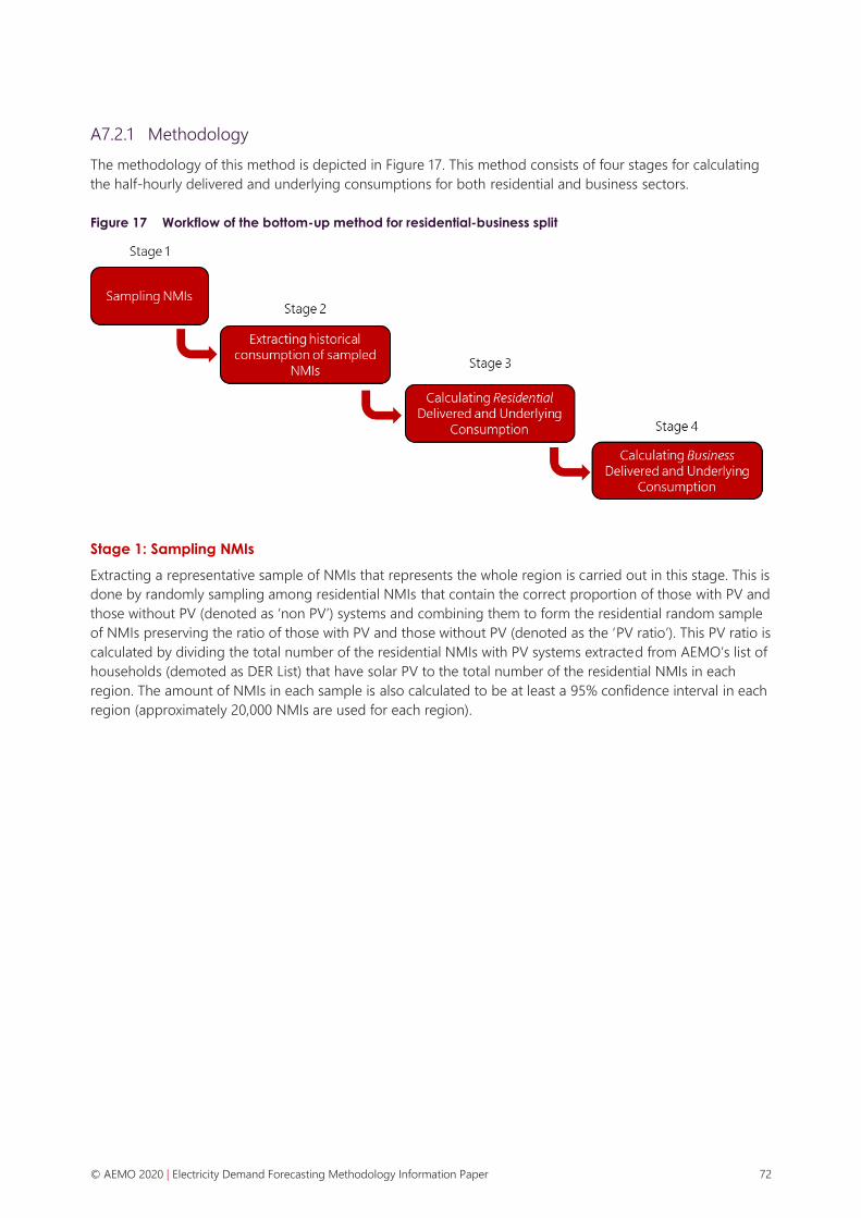
© AEMO 2020 | Electricity Demand Forecasting Methodology Information Paper 72
A7.2.1 Methodology
The methodology of this method is depicted in Figure 17. This method consists of four stages for calculating
the half-hourly delivered and underlying consumptions for both residential and business sectors.
Figure 17 Workflow of the bottom-up method for residential-business split
Stage 1: Sampling NMIs
Extracting a representative sample of NMIs that represents the whole region is carried out in this stage. This is
done by randomly sampling among residential NMIs that contain the correct proportion of those with PV and
those without PV (denoted as ‘non PV’) systems and combining them to form the residential random sample
of NMIs preserving the ratio of those with PV and those without PV (denoted as the ‘PV ratio’). This PV ratio is
calculated by dividing the total number of the residential NMIs with PV systems extracted from AEMO’s list of
households (demoted as DER List) that have solar PV to the total number of the residential NMIs in each
region. The amount of NMIs in each sample is also calculated to be at least a 95% confidence interval in each
region (approximately 20,000 NMIs are used for each region).

© AEMO 2020 | Electricity Demand Forecasting Methodology Information Paper 73
Stage 2: Extracting historical consumption of sampled NMIs
In this stage, the historical consumption from the sampled NMIs is extracted from AEMO’s database at the
half-hourly level.
Stage 3: Calculating residential delivered and underlying consumptions
The residential delivered and underlying consumption are calculated in this stage. The usage per NMI is
initially calculated from the sampled NMIs and then, using the count of connected residential NMIs (number
of households) in each region, the usage per NMI is scaled to produce the sample-derived regional
residential delivered consumption. Lastly, the residential underlying consumption is calculated by adding
residential PV generation as estimated for each region (refer to Appendix A3) to the residential delivered
consumption.
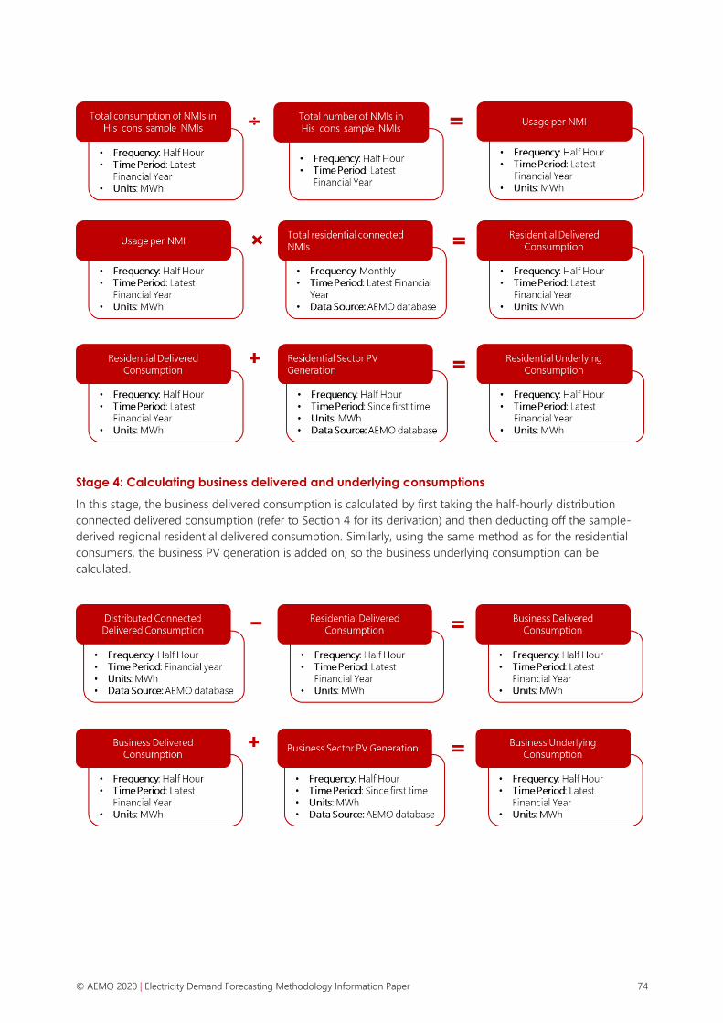
© AEMO 2020 | Electricity Demand Forecasting Methodology Information Paper 74
Stage 4: Calculating business delivered and underlying consumptions
In this stage, the business delivered consumption is calculated by first taking the half-hourly distribution
connected delivered consumption (refer to Section 4 for its derivation) and then deducting off the sample-
derived regional residential delivered consumption. Similarly, using the same method as for the residential
consumers, the business PV generation is added on, so the business underlying consumption can be
calculated.

© AEMO 2020 | Electricity Demand Forecasting Methodology Information Paper 75
A8. Demand trace scaling algorithm
This appendix provides a worked example of how half-hourly demand traces are scaled for the outlook
period. This covers the first two passes of the method described in Section 6.
The example begins with a financial-year time series of demand to be scaled to predefined targets. It has
been prepared by taking demand from a reference year and converting the values to OPSO-lite (removing
influence of PV, other non-scheduled generation, CSG, ESS and EVs). The example trace is presented in Figure
18.
Figure 18 Prepared demand trace
Day swapping is performed to exchange weekend and holiday dates between the reference year and the
forecast year. In this example, day swapping is assumed to have taken place.
The targets are summarised in 0. All targets represent an increase to the reference trace in this example.

© AEMO 2020 | Electricity Demand Forecasting Methodology Information Paper 76
Table 22 Prepared demand trace and targets
Prepared trace Target Unit
Summer Max 1063.231 1148.29 MW
Winter Max 911.79 938.33 MW
Minimum 466.695 488.695 MW
Energy 5733.727 6364.407 GWh
The series is categorised into n highest-demand days in summer (using daily maximum as the reference), n
highest demand days in winter, p lowest demand half-hour periods. In this example,
n = 10 days
p = 70 half-hour periods
The day-type categorisation (High Summer, High Winter, Low Period and Other) is displayed in Figure 19.
Figure 19 Day-type categories
Scaling then commences. The demand, categorised into day-types, is scaled according to the ratios in Table
23. The ratios are calculated as target / prepared trace using the information from 0.
Table 23 Scaling ratios
Day-type category Prepared trace Unit Target/Base ratio
Summer high days 169.81 GWh 1.080000
Winter high days 166.53 GWh 1.029108
Low periods 35.37 GWh 1.047140
The scaling ratios for the key day-type categories are based on maximum or minimum demand targets.
Therefore, the maximum demand and minimum demand targets are met by applying this process. Note that
the energy target still needs to be addressed. Application of the scaling factors results in the energy

© AEMO 2020 | Electricity Demand Forecasting Methodology Information Paper 77
presented in Table 24 and the remaining energy difference is calculated as the target minus the current grown
total.
Table 24 Resulting energy
Resulting GWh Units
Summer high days 183.40 GWh
Winter high days 171.38 GWh
Low periods 37.04 GWh
Remaining energy difference 610.58 GWh
The remaining energy difference from Table 24 equates to an 11.38% increase on the ‘other’ category’s
energy. This is applied to the demand in the other category and the targets are checked. The check is
summarised in Table 25 and the grown trace is plotted in Figure 20.
Figure 20 Grown trace and targets
Table 25 Check of grown trace against targets
Base trace Target Grown Units
Summer Max 1063.231 1148.29 1148.29 MW
Winter Max 911.79 938.33 957.54 MW
Minimum 466.695 488.695 488.695 MW
Energy 5733.727 6364.407 6364.407 GWh

© AEMO 2020 | Electricity Demand Forecasting Methodology Information Paper 78
The check summarised in Table 25 uncovers an inconsistency between the grown winter maximum and the
target (bold highlight). This was caused by the allocation of energy in the ‘other’ category which increased
some winter values above the initial peak.
In accordance with the methodology, the process is repeated until the targets are met.
Following completion of this first-pass growing process, and in accordance with the methodology, the
forecast technology components are added back to the trace to derive the unreconciled OPSO trace. Each
component-trace is prepared to reflect the forecast capacities or numbers in the target year and the nominal
or normalised power trace (from the reference year). In this way, the influence of PV, other non-scheduled
generation, CSG, ESS and EVs is appropriately applied to each half hour to derive the unreconciled OPSO
trace.
The growing process is then repeated on the unreconciled OPSO trace as per the ‘second pass’ of the
methodology. Demand and energy targets are changed accordingly to reflect demand being on the OPSO
basis.
EVs that can act as home batteries were modelled for the first time in the 2019 Step Change scenario. To
model this, a certain proportion of the residential vehicle fleet are modelled to have their EVs discharge in the
home (termed vehicle-to-home) to serve the users energy requirements. This discharge profile is included in
the demand trace growing algorithm in a similar way as the other behind the meter technologies. The charge
profile is not captured within the demand traces but is instead optimally charged within the supply model,
similar to VPP charging. In this way, the EV fleet charges from the grid at times of low system cost, avoiding
contribution to maximum demand.

© AEMO 2020 | Electricity Demand Forecasting Methodology Information Paper 79
Abbreviations
Abbreviation Full name
ABS Australian Bureau of Statistics
AER Australian Energy Regulator
BoM Bureau of Meteorology
CD Cooling degree
CDD Cooling degree day
CDF Cumulative density function
CER Clean Energy Regulator
COP Coefficient of performance
CSG Coal seam gas
DER Distributed energy resource
DSP Demand side participation
DBT Dry-bulb temperature
EDA Exploratory data analysis
EDD Effective degree day
ESS Energy storage systems
EV Electric vehicle
FiTs Feed-in tariffs
GFC Global Financial Crisis
GWh Gigawatt hours
HD Heating degree
HIA Housing Industry Association
HDD Heating degree day
ISP Integrated System Plan
KW Kilowatts
LIL Large industrial loads
LNG Liquefied natural gas

© AEMO 2020 | Electricity Demand Forecasting Methodology Information Paper 80
Abbreviation Full name
MD Maximum demand
MMS Market Management System
MW Megawatts
NEM National Electricity Market
NMI National meter identifier
NSG Non-scheduled generation
OLS Ordinary least squares
ONSG Other non-scheduled generators
OPSO Operational demand as sent out
POE Probability of exceedance
PVNSG PV non-scheduled generators
PVROOF Rooftop PV
STCs Small-scale technology certificates
VPP Virtual power plant
WBT Wet-bulb temperature