Self-similar solutions of the one-dimensional

Landau–Lifshitz–Gilbert equation

Susana Gutiérrez1 and André de Laire2

Abstract

We consider the one-dimensional Landau–Lifshitz–Gilbert (LLG) equation, a model des-cribing the dynamics for the spin in ferromagnetic materials. Our main aim is the analyticalstudy of the bi-parametric family of self-similar solutions of this model. In the presence ofdamping, our construction provides a family of global solutions of the LLG equation whichare associated to a discontinuous initial data of infinite (total) energy, and which are smoothand have finite energy for all positive times. Special emphasis will be given to the behaviourof this family of solutions with respect to the Gilbert damping parameter.

We would like to emphasize that our analysis also includes the study of self-similar so-lutions of the Schrödinger map and the heat flow for harmonic maps into the 2-sphere asspecial cases. In particular, the results presented here recover some of the previously knownresults in the setting of the 1d-Schrödinger map equation.Keywords and phrases: Landau–Lifshitz–Gilbert equation, Landau–Lifshitz equation, ferro-magnetic spin chain, Schrödinger maps, heat-flow for harmonic maps, self-similar solutions,asymptotics.

Contents

1 Introduction and statement of results 2

2 Self-similar solutions of the LLG equation 10

3 Integration of the Serret–Frenet system 12

3.1 Reduction to the study of a second order ODE . . . . . . . . . . . . . . . . . . . 12

3.2 The second-order equation. Asymptotics . . . . . . . . . . . . . . . . . . . . . . . 15

3.3 The second-order equation. Dependence on the parameters . . . . . . . . . . . . 28

3.3.1 Dependence on α . . . . . . . . . . . . . . . . . . . . . . . . . . . . . . . . 28

3.3.2 Dependence on c0 . . . . . . . . . . . . . . . . . . . . . . . . . . . . . . . . 33

4 Proof of the main results 34

5 Some numerical results 37

6 Appendix 41

1School of Mathematics, University of Birmingham, Edgbaston, Birmingham, B15 2TT, United Kingdom.E-mail: s.gutierrez@bham.ac.uk

2Laboratoire Paul Painlevé, Université Lille 1, 59655 Villeneuve d’Ascq Cedex, France. E-mail:andre.de-laire@math.univ-lille1.fr

1

1 Introduction and statement of results

In this work we consider the one-dimensional Landau–Lifshitz–Gilbert equation (LLG)

∂t~m = β~m× ~mss − α~m× (~m× ~mss), s ∈ R, t > 0, (LLG)

where ~m = (m1,m2,m3) : R × (0,∞) −→ S2 is the spin vector, β ≥ 0, α ≥ 0, × denotes the

usual cross-product in R3, and S

2 is the unit sphere in R3.

Here we have not included the effects of anisotropy or an external magnetic field. The first termon the right in (LLG) represents the exchange interaction, while the second one corresponds to theGilbert damping term and may be considered as a dissipative term in the equation of motion. Theparameters β ≥ 0 and α ≥ 0 are the so-called exchange constant and Gilbert damping coefficient,and take into account the exchange of energy in the system and the effect of damping on thespin chain respectively. Note that, by considering the time-scaling ~m(s, t) → ~m(s, (α2+β2)1/2t),in what follows we will assume w.l.o.g. that

α, β ∈ [0, 1] and α2 + β2 = 1. (1.1)

The Landau–Lifshitz–Gilbert equation was first derived on phenomenological grounds by L. Lan-dau and E. Lifshitz to describe the dynamics for the magnetization or spin ~m(s, t) in ferromag-netic materials [24, 11]. The nonlinear evolution equation (LLG) is related to several physicaland mathematical problems and it has been seen to be a physically relevant model for severalmagnetic materials [19, 20]. In the setting of the LLG equation, of particular importance is toconsider the effect of dissipation on the spin [27, 7, 6].

The Landau–Lifshitz family of equations includes as special cases the well-known heat-flowfor harmonic maps and the Schrödinger map equation onto the 2-sphere. Precisely, when β = 0(and therefore α = 1) the LLG equation reduces to the one-dimensional heat-flow equation forharmonic maps

∂t~m = −~m× (~m × ~mss) = ~mss + |~ms|2~m (HFHM)

(notice that |~m|2 = 1, and in particular ~m · ~mss = −|~ms|2). The opposite limiting case of theLLG equation (that is α = 0, i.e. no dissipation/damping and therefore β = 1) corresponds tothe Schrödinger map equation onto the sphere

∂t~m = ~m× ~mss. (SM)

Both special cases have been objects of intense research and we refer the interested reader to[21, 14, 25, 13] for surveys.

Of special relevance is the connection of the LLG equation with certain non-linear Schrödingerequations. This connection is established as follows: Let us suppose that ~m is the tangent vectorof a curve in R

3, that is ~m = ~Xs, for some curve ~X(s, t) ∈ R3 parametrized by the arc-length. It

can be shown [7] that if ~m evolves under (LLG) and we define the so-called filament function uassociated to ~X(s, t) by

u(s, t) = c(s, t)ei∫ s0 τ(σ,t) dσ, (1.2)

in terms of the curvature c and torsion τ associated to the curve, then u solves the followingnon-local non-linear Schrödinger equation with damping

iut + (β − iα)uss +u

2

(

β|u|2 + 2α

∫ s

0Im(uus)−A(t)

)

= 0, (1.3)

where A(t) ∈ R is a time-dependent function defined in terms of the curvature and torsionand their derivatives at the point s = 0. The transformation (1.2) was first considered in the

2

undamped case by Hasimoto in [18]. Notice that if α = 0, equation (1.3) can be transformedinto the well-known completely integrable cubic Schrödinger equation.

The main purpose of this paper is the analytical study of self-similar solutions of the LLGequation of the form

~m(s, t) = ~m

(

s√t

)

, (1.4)

for some profile ~m : R → S2, with emphasis on the behaviour of these solutions with respect to

the Gilbert damping parameter α ∈ [0, 1].

For α = 0, self-similar solutions have generated considerable interest [22, 21, 4, 15, 9]. We arenot aware of any other study of such solutions for α > 0 in the one dimensional case (see [10]for a study of self-similar solutions of the harmonic map flow in higher dimensions). However,Lipniacki [26] has studied self-similar solutions for a related model with nonconstant arc-length.On the other hand, little is known analytically about the effect of damping on the evolutionof a one-dimensional spin chain. In particular, Lakshmanan and Daniel obtained an explicitsolitary wave solution in [7, 6] and demonstrated the damping of the solution in the presenceof dissipation in the system. In this setting, we would like to understand how the dynamics ofself-similar solutions to this model is affected by the introduction of damping in the equationsgoverning the motion of these curves.

As will be shown in Section 2 self-similar solutions of (LLG) of the type (1.4) constitute abi-parametric family of solutions {~mc0,α}c0,α given by

~mc0,α(s, t) = ~mc0,α

(

s√t

)

, c0 > 0, α ∈ [0, 1], (1.5)

where ~mc0,α is the solution of the Serret–Frenet equations

~m′ = c~n,

~n′ = −c~m+ τ~b,

~b′ = −τ~n,(1.6)

with curvature and torsion given respectively by

cc0,α(s) = c0e−αs2

4 , τc0,α(s) =βs

2, (1.7)

and initial conditions

~mc0,α(0) = (1, 0, 0), ~nc0,α(0) = (0, 1, 0), ~bc0,α(0) = (0, 0, 1). (1.8)

The first result of this paper is the following:

Theorem 1.1. Let α ∈ [0, 1], c0 > 01 and ~mc0,α be the solution of the Serret–Frenet system(1.6) with curvature and torsion given by (1.7) and initial conditions (1.8). Define ~mc0,α(s, t) by

~mc0,α(s, t) = ~mc0,α

(

s√t

)

, t > 0.

Then,

1The case c0 = 0 corresponds to the constant solution for (LLG), that is

~mc0,α(s, t) = ~m

(

s√t

)

= (1, 0, 0), ∀α ∈ [0, 1].

3

(i) The function ~mc0,α(·, t) is a regular C∞(R;S2)-solution of (LLG) for t > 0.

(ii) There exist unitary vectors ~A±c0,α = (A±

j,c0,α)3j=1 ∈ S

2 such that the following pointwiseconvergence holds when t goes to zero:

limt→0+

~mc0,α(s, t) =

~A+c0,α, if s > 0,

~A−c0,α, if s < 0,

(1.9)

where ~A−c0,α = (A+

1,c0,α,−A+

2,c0,α,−A+

3,c0,α).

(iii) Moreover, there exists a constant C(c0, α, p) such that for all t > 0

‖~mc0,α(·, t)− ~A+c0,αχ(0,∞)(·)− ~A−

c0,αχ(−∞,0)(·)‖Lp(R) ≤ C(c0, α, p)t12p , (1.10)

for all p ∈ (1,∞). In addition, if α > 0, (1.10) also holds for p = 1. Here, χE denotes thecharacteristic function of a set E.

The graphics in Figure 1 depict the profile ~mc0,α(s) for fixed c0 = 0.8 and the values ofα = 0.01, α = 0.2, and α = 0.4. In particular it can be observed how the convergence of ~mc0,α

to ~A±c0,α is accelerated by the diffusion α.

m1m2

m3

(a) α = 0.01

m1m2

m3

(b) α = 0.2

m1m2

m3

(c) α = 0.4

Figure 1: The profile ~mc0,α for c0 = 0.8 and different values of α.

Notice that the initial condition

~mc0,α(s, 0) =~A+c0,αχ(0,∞)(s) + ~A−

c0,αχ(−∞,0)(s), (1.11)

has a jump singularity at the point s = 0 whenever the vectors ~A+c0,α and ~A−

c0,α satisfy

~A+c0,α 6= ~A−

c0,α.

In this situation (and we will be able to prove analytically this is the case at least for certain rangesof the parameters α and c0, see Proposition 1.5 below), Theorem 1.1 provides a bi-parametricfamily of global smooth solutions of (LLG) associated to a discontinuous singular initial data(jump-singularity).

4

As has been already mentioned, in the absence of damping (α = 0), singular self-similarsolutions of the Schrödinger map equation were previously obtained in [15], [22] and [4]. In thisframework, Theorem 1.1 establishes the persistence of a jump singularity for self-similar solutionsin the presence of dissipation.

Some further remarks on the results stated in Theorem 1.1 are in order. Firstly, from theself-similar nature of the solutions ~mc0,α(s, t) and the Serret–Frenet equations (1.6), it followsthat the curvature and torsion associated to these solutions are of the self-similar form and givenby

cc0,α(s, t) =c0√te−

αs2

4t and τc0,α(s, t) =βs

2√t. (1.12)

As a consequence, the total energy E(t) of the spin ~mc0,α(s, t) found in Theorem 1.1 is expressedas

E(t) =1

2

∫ ∞

−∞|~ms(s, t)|2 ds =

1

2

∫ ∞

−∞c2c0,α(s, t) ds

=1

2

∫ ∞

−∞

(

c0√te−

αs2

4t

)2

ds = c20

√

π

αt, α > 0, t > 0. (1.13)

It is evident from (1.13) that the total energy of the spin chain at the initial time t = 0 is infinite,while the total energy of the spin becomes finite for all positive times, showing the dissipationof energy in the system in the presence of damping.

Secondly, it is also important to remark that in the setting of Schrödinger equations, for fixedα ∈ [0, 1] and c0 > 0, the solution ~mc0,α(s, t) of (LLG) established in Theorem 1.1 is associatedthrough the Hasimoto transformation (1.2) to the filament function

uc0,α(s, t) =c0√te(−α+iβ) s

2

4t , (1.14)

which solves

iut + (β − iα)uss +u

2

(

β|u|2 + 2α

∫ s

0Im(uus)−A(t)

)

= 0, with A(t) =βc20t

(1.15)

and is such that at initial time t = 0

uc0,α(s, 0) = 2c0√

π(α+ iβ)δ0.

Here δ0 denotes the delta distribution at the point s = 0 and√z denotes the square root of a

complex number z such that Im(√z) > 0.

Notice that the solution uc0,α(s, t) is very rough at initial time, and in particular uc0,α(s, 0)does not belong to the Sobolev class Hs for any s ≥ 0. Therefore, the standard arguments (thatis a Picard iteration scheme based on Strichartz estimates and Sobolev-Bourgain spaces) cannotbe applied at least not in a straightforward way to study the local well-posedness of the initialvalue problem for the Schrödinger equations (1.15). The existence of solutions of the Scrödingerequations (1.15) associated to an initial data proportional to a Dirac delta opens the questionof developing a well-posedness theory for Schrödinger equations of the type considered here toinclude initial data of infinite energy. This question was addressed by A. Vargas and L. Vegain [29] and A. Grünrock in [12] in the case α = 0 and when A(t) = 0 (see also [2] for a relatedproblem), but we are not aware of any results in this setting when α > 0 (see [14] for relatedwell-posedness results in the case α > 0 for initial data in Sobolev spaces of positive index).Notice that when α > 0 , the solution (1.14) has infinite energy at the initial time, however the

5

energy becomes finite for any t > 0. Moreover, as a consequence of the exponential decay in thespace variable when α > 0, uc0,α(t) ∈ Hm(R), for all t > 0 and m ∈ N. Hence these solutions donot fit into the usual functional framework for solutions of the Schrödinger equations (1.15).

As already mentioned, one of the main goals of this paper is to study both the qualitative andquantitative effect of the damping parameter α and the parameter c0 on the dynamical behaviourof the family {~mc0,α}c0,α of self-similar solutions of (LLG) found in Theorem 1.1. Precisely, in anattempt to fully understand the regularization of the solution at positive times close to the initialtime t = 0, and to understand how the presence of damping affects the dynamical behaviour ofthese self-similar solutions, we aim to give answers to the following questions:

Q1: Can we obtain a more precise behaviour of the solutions ~mc0,α(s, t) at positive times t closeto zero?

Q2: Can we understand the limiting vectors ~A±c0,α in terms of the parameters c0 and α?

In order to address our first question, we observe that, due to the self-similar nature of thesesolutions (see (1.5)), the behaviour of the family of solutions ~mc0,α(s, t) at positive times close tothe initial time t = 0 is directly related to the study of the asymptotics of the associated profile~mc0,α(s) for large values of s. In addition, the symmetries of ~mc0,α(s) (see Theorem 1.2 below)allow to reduce ourselves to obtain the behaviour of the profile ~mc0,α(s) for large positive valuesof the space variable. The precise asymptotics of the profile is given in the following theorem.

Theorem 1.2 (Asymptotics). Let α ∈ [0, 1], c0 > 0 and {~mc0,α, ~nc0,α,~bc0,α} be the solution of

the Serret–Frenet system (1.6) with curvature and torsion given by (1.7) and initial conditions(1.8). Then,

(i) (Symmetries). The components of ~mc0,α(s), ~nc0,α(s) and ~bc0,α(s) satisfy respectively that

• m1,c0,α(s) is an even function, and mj,c0,α(s) is an odd function for j ∈ {2, 3}.• n1,c0,α(s) and b1,c0,α(s) are odd functions, while nj,c0,α(s) and bj,c0,α(s) are even func-

tions for j ∈ {2, 3}.

(ii) (Asymptotics). There exist an unit vector ~A+c0,α ∈ S

2 and ~B+c0,α ∈ R

3 such that the following

asymptotics hold for all s ≥ s0 = 4√

8 + c20:

~mc0,α(s) =~A+c0,α − 2c0

s~B+c0,αe

−αs2/4(α sin(~φ(s)) + β cos(~φ(s)))

− 2c20s2

~A+c0,αe

−αs2/2 +O

(

e−αs2/4

s3

)

, (1.16)

~nc0,α(s) =~B+c0,α sin(

~φ(s)) +2c0s~A+c0,ααe

−αs2/4 +O

(

e−αs2/4

s2

)

, (1.17)

~bc0,α(s) =~B+c0,α cos(

~φ(s)) +2c0s~A+c0,αβe

−αs2/4 +O

(

e−αs2/4

s2

)

. (1.18)

Here, sin(~φ) and cos(~φ) are understood acting on each of the components of ~φ = (φ1, φ2, φ3),with

φj(s) = aj + β

∫ s2/4

s20/4

√

1 + c20e−2ασ

σdσ, j ∈ {1, 2, 3}, (1.19)

6

for some constants a1, a2, a3 ∈ [0, 2π), and the vector ~B+c0,α is given in terms of ~A+

c0,α =

(A+j,c0,α

)3j=1 by

~B+c0,α = ((1− (A+

1,c0,α)2)1/2, (1− (A+

2,c0,α)2)1/2, (1− (A+

3,c0,α)2)1/2).

As we will see in Section 2, the convergence and rate of convergence of the solutions ~mc0,α(s, t)of the LLG equation established in parts (ii) and (iii) of Theorem 1.1 will be obtained as a con-sequence of the more refined asymptotic analysis of the associated profile given in Theorem 1.2.

With regard to the asymptotics of the profile established in part (ii) of Theorem 1.2, it isimportant to mention the following:

(a) The errors in the asymptotics in Theorem 1.2-(ii) depend only on c0. In other words,the bounds for the errors terms are independent of α ∈ [0, 1]. More precisely, we use thenotation O(f(s)) to denote a function for which exists a constant C(c0) > 0 depending onc0, but independent on α, such that

|O (f(s))| ≤ C(c0)|f(s)|, for all s ≥ s0. (1.20)

(b) The terms ~A+c0,α, ~B+

c0,α, B+j sin(aj) and B+

j cos(aj), j ∈ {1, 2, 3}, and the error terms inTheorem 1.2-(ii) depend continuously on α ∈ [0, 1] (see Subsection 3.3 and Corollary 3.14).Therefore, the asymptotics (1.16)–(1.18) show how the profile ~mc0,α converges to ~mc0,0 asα→ 0+ and to ~mc0,1 as α→ 1−. In particular, we recover the asymptotics for ~mc0,0 givenin [15].

(c) We also remark that using the Serret–Frenet formulae and the asymptotics in Theorem 1.2-(ii), it is straightforward to obtain the asymptotics for the derivatives of ~mc0,α(s, t).

(d) When α = 0 and for fixed j ∈ {1, 2, 3}, we can write φj in (1.19) as

φj(s) = aj +s2

4+ c20 ln(s) + C(c0) +O

(

1

s2

)

,

and we recover the logarithmic contribution in the oscillation previously found in [15].Moreover, in this case the asymptotics in part (ii) represents an improvement of the oneestablished in Theorem 1 in [15].

When α > 0, φj behaves like

φj(s) = aj +βs2

4+ C(α, c0) +O

(

e−αs2/2

αs2

)

, (1.21)

and there is no logarithmic correction in the oscillations in the presence of damping.

Consequently, the phase function ~φ defined in (1.19) captures the different nature of theoscillatory character of the solutions in both the absence and the presence of damping inthe system of equations.

(e) When α = 1, there exists an explicit formula for ~mc0,1, ~nc0,1 and ~bc0,1, and in particularwe have explicit expressions for the vectors ~A±

c0,1in terms of the parameter c0 > 0 in the

asymptotics given in part (ii). See Appendix.

7

(f) At first glance, one might think that the term −2c20~A+c0,αe

−αs2/2/s2 in (1.16) could be

included in the error term O(e−αs2/4/s3). However, we cannot do this because

e−αs2/2

s2>e−αs2/4

s3, for all 2 ≤ s ≤

(

2

3α

)1/2

, α ∈ (0, 1/8], (1.22)

and in our notation the big-O must be independent of α. (The exact interval where theinequality in (1.22) holds can be determined using the so-called Lambert W function.)

(g) Let ~B+c0,α,sin

= (Bj sin(aj))3j=1, ~B+

c0,α,cos = (Bj cos(aj))3j=1. Then the orthogonality of

~mc0,α, ~nc0,α and ~bc0,α together with the asymptotics (1.16)–(1.18) yield

~A+c0,α · ~B+

c0,α,sin= ~A+

c0,α · ~B+c0,α,cos =

~B+c0,α,sin

· ~B+c0,α,cos = 0,

which gives relations between the phases.

(h) Finally, the amplitude of the leading order term controlling the wave-like behaviour of thesolution ~mc0,α(s) around ~A±

c0,α for values of s sufficiently large is of the order c0 e−αs2/4/s,

from which one observes how the convergence of the solution to its limiting values ~A±c0,α is

accelerated in the presence of damping in the system. See Figure 1.

We conclude the introduction by stating the results answering the second of our questions. Pre-cisely, Theorems 1.3 and 1.4 below establish the dependence of the vectors ~A±

c0,α in Theorem 1.1with respect to the parameters α and c0. Theorem 1.3 provides the behaviour of the limitingvector ~A+

c0,α for a fixed value of α ∈ (0, 1) and “small” values of c0 > 0, while Theorem 1.4 states

the behaviour of ~A+c0,α for fixed c0 > 0 and α close to the limiting values α = 0 and α = 1. Recall

that ~A−c0,α is expressed in terms of the coordinates of ~A+

c0,α as

~A−c0,α = (A+

1,c0,α,−A+

2,c0,α,−A+

3,c0,α) (1.23)

(see part (ii) of Theorem 1.1).

Theorem 1.3. Let α ∈ [0, 1], c0 > 0, and ~A+c0,α = (A+

j,c0,α)3j=1 be the unit vector given in

Theorem 1.2. Then ~A+c0,α is a continuous function of c0 > 0. Moreover, if α ∈ (0, 1] the

following inequalities hold true:

|A+1,c0,α

− 1| ≤ c20π

α

(

1 +c20π

8α

)

, (1.24)

∣

∣

∣

∣

∣

A+2,c0,α

− c0

√

π(1 + α)√2

∣

∣

∣

∣

∣

≤ c20π

4+

c20π

α√2

(

1 +c20π

8+ c0

√

π(1 + α)

2√2

)

+

(

c20π

2√2α

)2

, (1.25)

∣

∣

∣

∣

∣

A+3,c0,α

− c0

√

π(1− α)√2

∣

∣

∣

∣

∣

≤ c20π

4+

c20π

α√2

(

1 +c20π

8+ c0

√

π(1− α)

2√2

)

+

(

c20π

2√2α

)2

. (1.26)

The following result provides an approximation of the behaviour of ~A+c0,α for fixed c0 > 0 and

values of the Gilbert parameter close to 0 and 1.

Theorem 1.4. Let c0 > 0, α ∈ [0, 1] and ~A+c0,α be the unit vector given in Theorem 1.2. Then

~A+c0,α is a continuous function of α in [0, 1], and the following inequalities hold true:

| ~A+c0,α − ~A+

c0,0| ≤ C(c0)

√α| ln(α)|, for all α ∈ (0, 1/2], (1.27)

| ~A+c0,α − ~A+

c0,1| ≤ C(c0)

√1− α, for all α ∈ [1/2, 1]. (1.28)

Here, C(c0) is a positive constant depending on c0 but otherwise independent of α.

8

As a by-product of Theorems 1.3 and 1.4, we obtain the following proposition which assertsthat the solutions ~mc0,α(s, t) of the LLG equation found in Theorem 1.1 are indeed associatedto a discontinuous initial data at least for certain ranges of α and c0.

Proposition 1.5. With the same notation as in Theorems 1.1 and 1.2, the following statementshold:

(i) For fixed α ∈ (0, 1) there exists c∗0 > 0 depending on α such that

~A+c0,α 6= ~A−

c0,α for all c0 ∈ (0, c∗0).

(ii) For fixed c0 > 0, there exists α∗0 > 0 small enough such that

~A+c0,α 6= ~A−

c0,α for all α ∈ (0, α∗0).

(iii) For fixed 0 < c0 6= k√π with k ∈ N, there exists α∗

1 > 0 with 1−α∗1 > 0 small enough such

that~A+c0,α 6= ~A−

c0,α for all α ∈ (α∗1, 1).

Remark 1.6. Based on the numerical results in Section 5, we conjecture that ~A+c0,α 6= ~A−

c0,α forall α ∈ [0, 1) and c0 > 0.

We would like to point out that some of our results and their proofs combine and extendseveral ideas previously introduced in [15] and [16]. The approach we use in the proof of themain results in this paper is based on the integration of the Serret–Frenet system of equationsvia a Riccati equation, which in turn can be reduced to the study of a second order ordinarydifferential equation given by

f ′′(s) +s

2(α+ iβ)f ′(s) +

c204e−

αs2

2 f(s) = 0 (1.29)

when the curvature and torsion are given by (1.7).

Unlike in the undamped case, in the presence of damping no explicit solutions are knownfor equation (1.29) and the term containing the exponential in the equation (1.29) makes itdifficult to use Fourier analysis methods to study analytically the behaviour of the solutions tothis equation. The fundamental step in the analysis of the behaviour of the solutions of (1.29)consists in introducing new auxiliary variables z, h and y defined by

z = |f |2, y = Re(ff ′) and h = Im(ff ′)

in terms of solutions f of (1.29), and studying the system of equations satisfied by these keyquantities. As we will see later on, these variables are the “natural” ones in our problem, in thesense that the components of the tangent, normal and binormal vectors can be written in termsof these quantities. It is important to emphasize that, in order to obtain error bounds in theasymptotic analysis independent of the damping parameter α (and hence recover the asymptoticswhen α = 0 and α = 1 as particular cases), it will be fundamental to exploit the cancellationsdue to the oscillatory character of z, y and h.

The outline of this paper is the following. Section 2 is devoted to the construction of the familyof self-similar solutions {~mc0,α}c0,α of the LLG equation. In Section 3 we reduce the study of theproperties of this family of self-similar solutions to that of the properties of the solutions of thecomplex second order complex ODE (1.29). This analysis is of independent interest. Section 4contains the proofs of the main results of this paper as a consequence of those established in

9

Section 3. In Section 5 we give provide some numerical results for ~A+c0,α, as a function of α ∈ [0, 1]

and c0 > 0, which give some inside for the scattering problem and justify Remark 1.6. Finally,we have included the study of the self-similar solutions of the LLG equation in the case α = 1in Appendix.

Acknowledgements. S. Gutiérrez and A. de Laire were supported by the British project“Singular vortex dynamics and nonlinear Schrödinger equations” (EP/J01155X/1) funded byEPSRC. S. Gutiérrez was also supported by the Spanish projects MTM2011-24054 and IT641-13.

Both authors would like to thank L. Vega for many enlightening conversations and for hiscontinuous support.

2 Self-similar solutions of the LLG equation

First we derive what we will refer to as the geometric representation of the LLG equation. Tothis end, let us assume that ~m(s, t) = ~Xs(s, t) for some curve ~X(s, t) in R

3 parametrized withrespect to the arc-length with curvature c(s, t) and torsion τ(s, t). Then, using the Serret–Frenetsystem of equations (1.6), we have

~mss = cs~n + c(−c~n + τ~b),

and thus we can rewrite (LLG) as

∂t~m = β(cs~b− cτ~n) + α(cτ~b + cs~n), (2.1)

in terms of intrinsic quantities c, τ and the Serret–Frenet trihedron {~m, ~n, ~b}.We are interested in self-similar solutions of (LLG) of the form

~m(s, t) = ~m

(

s√t

)

(2.2)

for some profile ~m : R −→ S2. First, notice that due to the self-similar nature of ~m(s, t) in (2.2),

from the Serret–Frenet equations (1.6) it follows that the unitary normal and binormal vectorsand the associated curvature and torsion are self-similar and given by

~n(s, t) = ~n

(

s√t

)

, ~b(s, t) = ~b

(

s√t

)

, (2.3)

c(s, t) =1√tc

(

s√t

)

and τ(s, t) =1√tτ

(

s√t

)

. (2.4)

Assume that ~m(s, t) is a solution of the LLG equation, or equivalently of its geometric version(2.1). Then, from (2.2)–(2.4) it follows that the Serret–Frenet trihedron {~m(·), ~n(·),~b(·)} solves

−s2c~n = β(c′~b− cτ~n) + α(cτ~b+ c′~n), (2.5)

As a consequence,

−s2c = αc′ − βcτ and βc′ + αcτ = 0.

Thus, we obtain

c(s) = c0 e−αs2

4 and τ(s) =βs

2, (2.6)

10

for some positive constant c0 (recall that we are assuming w.l.o.g. that α2 + β2 = 1). Therefore,in view of (2.4), the curvature and torsion associated to a self-similar solution of (LLG) of theform (2.2) are given respectively by

c(s, t) =c0√te−

αs2

4t and τ(s, t) =βs

2t, c0 > 0. (2.7)

Notice that given (c, τ) as above, for fixed time t > 0 one can solve the Serret–Frenet system ofequations to obtain the solution up to a rigid motion in the space which in general may dependon t. As a consequence, and in order to determine the dynamics of the spin chain, we needto find the time evolution of the trihedron {~m(s, t), ~n(s, t), ~b(s, t)} at some fixed point s∗ ∈ R.To this end, from the above expressions of the curvature and torsion associated to ~m(s, t) andevaluating the equation (2.1) at the point s∗ = 0, we obtain that ~mt(0, t) = ~0. On the otherhand, differentiating the geometric equation (2.1) with respect to s, and using the Serret–Frenetequations (1.6) together with the compatibility condition ~mst = ~mts, we get the following relationfor the time evolution of the normal vector

c~nt = β(css~b + c2τ~m− cτ2~b) + α((cτ)s~b− ccs~m+ csτ~b).

The evaluation of the above identity at s∗ = 0 together with the expressions for the curvatureand torsion in (2.7) yield ~nt(0, t) = ~0. The above argument shows that

~mt(0, t) = ~0, ~nt(0, t) = ~0 and ~bt(0, t) = (~m× ~n)t(0, t) = ~0.

Therefore we can assume w.l.o.g. that

~m(0, t) = (1, 0, 0), ~n(0, t) = (0, 1, 0) and ~b(0, t) = (0, 0, 1),

and in particular

~m(0) = ~m(0, 1) = (1, 0, 0), ~n(0) = ~n(0, 1) = (0, 1, 0), and ~b(0) = ~b(0, 1) = (0, 0, 1). (2.8)

Given α ∈ [0, 1] and c0 > 0, from the theory of ODE’s, it follows that there exists a unique{~mc0,α(·), ~nc0,α(·),~bc0,α(·)} ∈

(

C∞(R;S2))3

solution of the Serret–Frenet equations (1.6) withcurvature and torsion (2.6) and initial conditions (2.8) such that

~mc0,α ⊥ ~nc0,α, ~mc0,α ⊥ ~bc0,α, ~nc0,α ⊥ ~bc0,α

and|~mc0,α|2 = |~nc0,α|2 = |~bc0,α|2 = 1.

Define ~mc0,α(s, t) as

~mc0,α(s, t) = ~mc0,α

(

s√t

)

. (2.9)

Then, ~mc0,α(·, t) ∈ C∞ (R;S2

)

for all t > 0, and bearing in mind both the relations in (2.3)–(2.4)

and the fact that the vectors {~mc0,α(·), ~nc0,α(·),~bc0,α(·)} satisfy the identity (2.5), a straightfor-ward calculation shows that ~mc0,α(·, t) is a regular C∞(R;S2)-solution of the LLG equation forall t > 0. Notice that the case c0 = 0 yields the constant solution ~m0,α(s, t) = (1, 0, 0). Thereforein what follows we will assume that c0 > 0.

The rest of the paper is devoted to establish analytical properties of the solutions {~mc0,α(s, t)}c0,αdefined by (2.9) for fixed α ∈ [0, 1] and c0 > 0. As already mentioned, due to the self-similarnature of these solutions, it suffices to study the properties of the associated profile ~mc0,α(·) or,equivalently, of the solution {~mc0,α, ~nc0,α,

~bc0,α} of the Serret–Frenet system (1.6) with curvatureand torsion given by (2.6) and initial conditions (2.8). As we will continue to see, the analysisof the profile solution {~mc0,α, ~nc0,α,

~bc0,α} can be reduced to the study of the properties of thesolutions of a certain second order complex differential equation.

11

3 Integration of the Serret–Frenet system

3.1 Reduction to the study of a second order ODE

Classical changes of variables from the differential geometry of curves allow us to reduce the nineequations in the Serret–Frenet system into three complex-valued second order equations (see[8, 28, 23]). Theses changes of variables are related to stereographic projection and this approachwas also used in [15]. However, their choice of stereographic projection has a singularity at theorigin, which leads to an indetermination of the initial conditions of some of the new variables.For this reason, we consider in the following lemma a stereographic projection that is compatiblewith the initial conditions (2.8). Although the proof of the lemma below is a slight modificationof that in [23, Subsections 2.12 and 7.3], we have included its proof here both for the sake ofcompleteness and to clarify to the unfamiliar reader how the integration of the Frenet equationscan be reduced to the study of a second order differential equation.

Lemma 3.1. Let ~m = (mj(s))3j=1, ~n = (nj(s))

3j=1 and ~b = (bj(s))

3j=1 be a solution of the Serret–

Frenet equations (1.6) with positive curvature c and torsion τ . Then, for each j ∈ {1, 2, 3} thefunction

fj(s) = e12

∫ s0 c(σ)ηj (σ) dσ, with ηj(s) =

(nj(s) + ibj(s))

1 +mj(s),

solves the equation

f ′′j (s) +

(

iτ(s)− c′(s)

c(s)

)

f ′j(s) +c2(s)

4fj(s) = 0, (3.1)

with initial conditions

fj(0) = 1, f ′j(0) =c(0)(nj(0) + ibj(0))

2(1 +mj(0)).

Moreover, the coordinates of ~m, ~n and ~b are given in terms of fj and f ′j by

mj(s) = 2

(

1 +4

c(s)2

∣

∣

∣

∣

f ′j(s)

fj(s)

∣

∣

∣

∣

2)−1

− 1, nj(s) + ibj(s) =4f ′j(s)

c(s)fj(s)

(

1 +4

c(s)2

∣

∣

∣

∣

f ′j(s)

fj(s)

∣

∣

∣

∣

2)−1

.

(3.2)The above relations are valid at least as long as mj > −1 and |fj| > 0.

Proof. For simplicity, we omit the index j. The proof relies on several transformations that arerather standard in the study of curves. First we define the complex function

N = (n+ ib)ei∫ s0 τ(σ) dσ. (3.3)

Then N ′ = iτN + (n′ + ib′)ei∫ s0τ(σ) dσ . On the other hand, the Serret–Frenet equations imply

thatn′ + ib′ = −cm− iτNe−i

∫ s0 τ(σ) dσ .

Therefore, settingψ = cei

∫ s0 τ(σ) dσ,

we getN ′ = −ψm. (3.4)

Using again the Serret–Frenet equations, we also obtain

m′ =1

2(ψN + ψN ). (3.5)

12

Let us consider now the auxiliary function

ϕ =N

1 +m. (3.6)

Differentiating and using (3.4), (3.5) and (3.6)

ϕ′ =N ′

1 +m− Nm′

(1 +m)2

=N ′

1 +m− ϕm′

1 +m

= −ϕ2ψ

2− ψ

2(1 +m)(2m+ ϕN ).

Noticing that we can recast the relation m2+n2+ b2 = 1 as NN = (1−m)(1+m) and recallingthe definition of ϕ in (3.6), we have ϕN = 1−m, so that

ϕ′ +ϕ2ψ

2+ψ

2= 0. (3.7)

Finally, define the stereographic projection of (m,n, b) by

η =n+ ib

1 +m. (3.8)

Observe that from the definitions of N and ϕ, respectively in (3.3) and (3.6), we can rewrite ηas

η = ϕe−i∫ s0 τ(σ) dσ ,

and from (3.7) it follows that η solves the Riccati equation

η′ + iτη +c

2(η2 + 1) = 0, (3.9)

(recall that ψ = cei∫ s0 τ(σ) dσ). Finally, setting

f(s) = e12

∫ s0c(σ)η(σ) dσ , (3.10)

we get

η =2f ′

cf(3.11)

and equation (3.1) follows from (3.9). The initial conditions are an immediate consequence ofthe definition of η and f in (3.8) and (3.10).

A straightforward calculation shows that the inverse transformation of the stereographic pro-jection is

m =1− |η|21 + |η|2 , n =

2Re η

1 + |η|2 , b =2 Im η

1 + |η|2 ,

so that we obtain (3.2) using (3.11) and the above identities.

Going back to our problem, Lemma 3.1 reduces the analysis of the solution {~m,~n,~b} of theSerret–Frenet system (1.6) with curvature and torsion given by (2.6) and initial conditions (2.8)to the study of the second order differential equation

f ′′(s) +s

2(α+ iβ)f ′(s) +

c204e−αs2/2f(s) = 0, (3.12)

13

with three initial conditions: For (m1, n1, b1) = (1, 0, 0) the associated initial condition for f1 is

f1(0) = 1, f ′1(0) = 0, (3.13)

for (m2, n2, b2) = (0, 1, 0) is

f2(0) = 1, f ′2(0) =c02, (3.14)

and for (m3, n3, b3) = (0, 0, 1) is

f3(0) = 1, f ′3(0) =ic02. (3.15)

It is important to notice that, by multiplying (3.12) by f ′ and taking the real part, it is easy tosee that

d

ds

[

1

2

(

eαs2

2 |f ′|2 + c204|f |2

)]

= 0.

Thus,

E(s) :=1

2

(

eαs2

2 |f ′|2 + c204|f |2

)

= E0, ∀ s ∈ R, (3.16)

with E0 a constant defined by the value of E(s) at some point s0 ∈ R. The conservation of theenergy E(s) allows us to simplify the expressions of mj , nj and bj for j ∈ {1, 2, 3} in the formulae(3.2) in terms of the solution fj to (3.12) associated to the initial conditions (3.13)–(3.15).

Indeed, on the one hand notice that the energies associated to the initial conditions (3.13)–(3.15) are respectively

E0,1 =c208, E0,2 =

c204

and E0,3 =c204. (3.17)

On the other hand, from (3.16), it follows that

(

1 +4

c20e−αs2

2

|f ′j |2(s)|fj |2(s)

)−1

=c20

8E0,j|fj|2(s), j ∈ {1, 2, 3}.

Therefore, from (3.17), the above identity and formulae (3.2) in Lemma 3.1, we conclude that

m1(s) = 2|f1(s)|2 − 1, n1(s) + ib1(s) =4

c0eαs

2/4f1(s)f′1(s), (3.18)

mj(s) = |fj(s)|2 − 1, nj(s) + ibj(s) =2

c0eαs

2/4fj(s)f′j(s), j ∈ {2, 3}. (3.19)

The above identities give the expressions of the tangent, normal and binormal vectors in termsof the solutions {fj}3j=1 of the second order differential equation (3.12) associated to the initialconditions (3.13)–(3.15).

By Lemma 3.1, the formulae (3.18) and (3.19) are valid as long asmj > −1, which is equivalentto the condition |fj| 6= 0. As shown in Appendix, for α = 1 there is s > 0 such that mj(s) = −1and then (3.18) and (3.19) are (a priori) valid just in a bounded interval. However, the trihedron{~m,~n,~b} is defined globally and fj can also be extended globally as the solution of the linearequation (3.12). Then, it is simple to verify that the functions given by the l.h.s. of formulae(3.18) and (3.19) satisfy the Serret–Frenet system and hence, by the uniqueness of the solution,the formulae (3.18) and (3.19) are valid for all s ∈ R.

14

3.2 The second-order equation. Asymptotics

In this section we study the properties of the complex-valued equation

f ′′(s) +s

2(α+ iβ)f ′(s) +

c204f(s)e−αs2/2 = 0, (3.20)

for fixed c0 > 0, α ∈ [0, 1), β > 0 such that α2 + β2 = 1. We begin noticing that in thecase α = 0, the solution can be written explicitly in terms of parabolic cylinder functions orconfluent hypergeometric functions (see [1]). Another analytical approach using Fourier analysistechniques has been taken in [15], leading to the asymptotics

f(s) = C1ei(c20/2) ln(s) + C2

e−is2/4

se−i(c20/2) ln(s) +O(1/s2), (3.21)

as s→ ∞, where the constants C1, C2 and O(1/s2) depend on the initial conditions and c0.

For α = 1, equation (3.20) can be also solved explicitly and the solution is given by

f(s) =2f ′(0)

c0sin

(

c02

∫ s

0e−σ2/4 dσ

)

+ f(0) cos

(

c02

∫ s

0e−σ2/4 dσ

)

.

In the case α ∈ (0, 1), one cannot compute the solutions of (3.20) in terms of known functionsand we will follow a more analytical analysis. In contrast with the situation when α = 0, it isfar from evident to use Fourier analysis to study (3.20) when α > 0.

For the rest of this section we will assume that α ∈ [0, 1). In addition, we will also assume thats > 0 and we will develop the asymptotic analysis necessary to establish part (ii) of Theorem 1.2.At this point, it is important to recall the expressions given in (3.18)–(3.19) for the coordinatesof the tangent, normal and binormal vectors associated to our family of solutions of the LLGequation in terms f . Bearing this in mind, we observe that the study of the asymptotic behaviourof these vectors are dictated by the asymptotic behaviour of the variables

z = |f |2, y = Re(ff ′), and h = Im(f f ′) (3.22)

associated to the solution f of (3.20).

As explained in the remark (a) after Theorem 1.2, we need to work with remainder terms thatare independent of α. To this aim, we proceed in two steps: first we found uniform estimatesfor α ∈ [0, 1/2] in Propositions 3.2 and 3.3, then we treat the case α ∈ [1/2, 1) in Lemma 3.6. InSubsection 3.3 we provide some continuity results that allows us to take α → 1− and give thefull statement in Corollary 3.14. Finally, notice that these asymptotics lead to the asymptoticsfor the original equation (3.20) (see Remark 3.9).

We begin our analysis by establishing the following:

Proposition 3.2. Let c0 > 0, α ∈ [0, 1), β > 0 such that α2 + β2 = 1, and f be a solution of(3.20). Define z, y and h as z = |f |2 and y + ih = ff ′. Then

(i) There exists E0 ≥ 0 such that the identity

1

2

(

eαs2

2 |f ′|2 + c204|f |2

)

= E0

holds true for all s ∈ R. In particular, f , f ′, z, y and h are bounded functions. Moreover,for all s ∈ R

|f(s)| ≤√8E0

c0, |f ′(s)| ≤

√

2E0 e−αs2/4, (3.23)

|z(s)| ≤ 8E0

c20and |h(s)| + |y(s)| ≤ 8E0

c0e−αs2/4. (3.24)

15

(ii) The limitz∞ : = lim

s→∞z(s)

exists.

(iii) Let γ := 2E0 − c20z∞/2 and s0 = 4√

8 + c20. For all s ≥ s0, we have

z(s)− z∞ = −4

s(αy + βh)− 4γ

s2e−αs2/2 +R0(s), (3.25)

where

|R0(s)| ≤ C(E0, c0)e−αs2/4

s3. (3.26)

Proof. Part (i) is just the conservation of energy proved in (3.16). Next, using the conservationlaw in part (i), we obtain that the variables {z, y, h} solve the first-order real system

z′ = 2y, (3.27)

y′ = βs

2h− α

s

2y + e−αs2/2

(

2E0 −c202z

)

, (3.28)

h′ = −β s2y − α

s

2h. (3.29)

To show (ii), plugging (3.27) into (3.29) and integrating from 0 to some s > 0 we obtain

z(s)− 1

s

∫ s

0z(σ) dσ = − 4

βs

(

h(s)− h(0) +α

2

∫ s

0σh(σ) dσ

)

. (3.30)

Also, using the above identity,

d

ds

(

1

s

∫ s

0z(σ) dσ

)

= − 4

βs2

(

h(s)− h(0) +α

2

∫ s

0σh(σ) dσ

)

. (3.31)

Now, since from part (i) |h(s)| ≤ 8E0c0

e−αs2/4, both h and α∫ s0 σh(σ) dσ are bounded functions,

thus from (3.31) it follows that the limit of 1s

∫ s0 z exists, as s → ∞. Hence (3.30) and previous

observations conclude that the limit z∞ := lims→∞ z(s) exists and furthermore

z∞ := lims→∞

z(s) = lims→∞

1

s

∫ s

0z(σ). (3.32)

We continue to prove (iii). Integrating (3.31) between s > 0 and +∞ and using integrationby parts, we obtain

z∞ − 1

s

∫ s

0z(σ) dσ = − 4

β

∫ ∞

s

h(σ)

σ2dσ +

4

β

h(0)

s− 2α

β

[

1

s

∫ s

0σh(σ) dσ +

∫ ∞

sh(σ) dσ

]

. (3.33)

From (3.30) and (3.33), we get

z(s)− z∞ = − 4

β

h(s)

s+

2α

β

∫ ∞

sh(σ) dσ +

4

β

∫ ∞

s

h(σ)

σ2. (3.34)

In order to compute the integrals in (3.34), using (3.27) and (3.28), we write

h =2

β

(

y′

s+α

4z′ − 2E0

se−αs2/2 +

c202sze−αs2/2

)

.

16

Then, integrating by parts and using the bound for y in (3.24),

∫ ∞

sh(σ) =

2

β

(

−ys+

∫ ∞

s

y

σ2+α

4(z∞ − z)− 2E0

∫ ∞

s

e−ασ2/2

σ+c202

∫ ∞

s

z

σe−ασ2/2

)

. (3.35)

Also, from (3.27) and (3.34), we obtain

∫ ∞

s

h(σ)

σ2=

2

β

(

∫ ∞

s

y′

σ3+α

2

∫ ∞

s

y

σ2− 2E0

∫ ∞

s

e−ασ2/2

σ3+c202

∫ ∞

s

z

σ3e−ασ2/2

)

. (3.36)

Multiplying (3.34) by β2, using (3.35), (3.36) and the identity

α

∫ ∞

s

e−ασ2/2

σn=e−αs2/2

sn+1− (n+ 1)

∫ ∞

s

e−ασ2/2

σn+2, for all α ≥ 0, n ≥ 1,

we conclude that

(α2 + β2)(z − z∞) =− 4

s(αy + βh)− 8E0

s2e−αs2/2

+ 8α

∫ ∞

s

y

σ2+ 8

∫ ∞

s

y′

σ3+ 2c20

∫ ∞

se−ασ2/2z

(

α

σ+

2

σ3

)

. (3.37)

Finally, using (3.27) and the boundedness of z and y, an integration by parts argument showsthat

8α

∫ ∞

s

y

σ2+ 8

∫ ∞

s

y′

σ3= −4α

z

s2− 8

y

s3− 12

z

s4+ 8

∫ ∞

sz

(

α

σ3− 6

σ5

)

. (3.38)

Bearing in mind that α2 + β2 = 1, from (3.37) and (3.38), we obtain the following identity

z − z∞ =− 4

s(αy + βh)− 8E0

s2e−αs2/2 − 4α

z

s2− 8

y

s3− 12

z

s4+ 8

∫ ∞

sz

(

α

σ3+

6

σ5

)

dσ

+ 2c20

∫ ∞

se−ασ2/2z

(

α

σ+

2

σ3

)

dσ,

(3.39)

for all s > 0. In order to prove (iii), we first write z = z − z∞ + z∞ and observe that

8α

∫ ∞

s

z

σ3= 8α

∫ ∞

s

z − z∞σ3

+4αz∞s2

,

∫ ∞

s

z

σ5=

∫ ∞

s

z − z∞σ5

+z∞4s4

and∫ ∞

se−ασ2/2z

(

α

σ+

2

σ3

)

=

∫ ∞

se−ασ2/2(z − z∞)

(

α

σ+

2

σ3

)

+z∞s2e−αs2/2.

Therefore, we can recast (3.39) as (3.25) with

R0(s) =− 4α(z − z∞)

s2− 8y

s3− 12(z − z∞)

s4+ 8

∫ ∞

s(z − z∞)

(

α

σ3+

6

σ5

)

dσ

+ 2c20

∫ ∞

se−ασ2/2(z − z∞)

(

α

σ+

2

σ3

)

dσ.

(3.40)

Let us take s0 ≥ 1 to be fixed in what follows. For t ≥ s0, we denote ‖ · ‖t the norm ofL∞([t,∞)). From the definition of R0 in (3.40) and the elementary inequalities

α

∫ ∞

s

e−ασ2/2

σn≤ e−αs2/2

sn+1, for all α ≥ 0, n ≥ 1, (3.41)

17

and∫ ∞

s

e−ασ2/2

σn≤ e−αs2/2

(n− 1)sn−1, for all α ≥ 0, n > 1, (3.42)

we obtain

‖R0‖t ≤8‖y‖tt3

+4

t2

(

8 + c20e−αt2/2

)

‖z − z∞‖t.

Hence, choosing s0 = 4√

8 + c20, so that 4t2

(

8 + c20e−αt2/2

)

≤ 1/2, from (3.24) and (3.25) we

conclude that there exists a constant C(E0, c0) > 0 such that

‖z − z∞‖t ≤C(E0, c0)

te−αt2/4, for all α ∈ [0, 1) and t ≥ s0,

which implies that

|z(s)− z∞| ≤ C(E0, c0)

se−αs2/4, for all α ∈ [0, 1), s ≥ s0. (3.43)

Finally, plugging (3.24) and (3.43) into (3.40) and bearing in mind the inequalities (3.41) and(3.42), we deduce that

|R0(s)| ≤ C(E0, c0)e−αs2/4

s3, ∀ s ≥ s0 = 4

√

8 + c20, (3.44)

and the proof of (iii) is completed.

Formula (3.25) in Proposition 3.2 gives z in terms of y and h. Therefore, we can reduce ouranalysis to that of the variables y and h or, in other words, to that of the system (3.27)–(3.29).In fact, a first attempt could be to define w = y + ih, so that from (3.28) and (3.29), we havethat w solves

(

we(α+iβ)s2/4)′

= e(−α+iβ)s2/4

(

γ − c202(z − z∞)

)

. (3.45)

From (3.43) in Proposition 3.2 and (3.45), we see that the limit w∗ = lims→∞w(s)e(α+iβ)s2/4

exists (at least when α 6= 0), and integrating (3.45) from some s > 0 to ∞ we find that

w(s) = e−(α+iβ)s2/4

(

w∗ −∫ ∞

se(−α+iβ)σ2/4

(

γ − c202(z − z∞)

)

dσ

)

.

In order to obtain an asymptotic expansion, we need to estimate∫∞s e(−α+iβ)σ2/4(z − z∞), for s

large. This can be achieved using (3.43),∣

∣

∣

∣

∫ ∞

se(−α+iβ)σ2/4(z − z∞) dσ

∣

∣

∣

∣

≤ C(E0, c0)

∫ ∞

s

e−ασ2/2

σdσ (3.46)

and the asymptotic expansion

∫ ∞

s

e−ασ2/2

σdσ = e−αs2/2

(

1

αs2− 2

α2s4+

8

α3s6+ · · ·

)

.

However this estimate diverges as α → 0. The problem is that the bound used in obtaining(3.46) does not take into account the cancellations due to the oscillations. Therefore, and inorder to obtain the asymptotic behaviour of z, y and h valid for all α ∈ [0, 1), we need a morerefined analysis. In the next proposition we study the system (3.27)–(3.29), where we considerthe cancellations due the oscillations (see Lemma 3.5 below). The following result providesestimates that are valid for s ≥ s1, for some s1 independent of α, if α is small.

18

Proposition 3.3. With the same notation and terminology as in Proposition 3.2, let

s1 = max

{

4√

8 + c20, 2c0

(

1

β− 1

)1/2}

.

Then for all s ≥ s1,

y(s) = be−αs2/4 sin(φ(s1; s))−2αγ

se−αs2/2 +O

(

e−αs2/2

β2s2

)

, (3.47)

h(s) = be−αs2/4 cos(φ(s1; s))−2βγ

se−αs2/2 +O

(

e−αs2/2

β2s2

)

, (3.48)

where

φ(s1; s) = a+ β

∫ s2/4

s21/4

√

1 + c20e−2αt

tdt,

a ∈ [0, 2π) is a real constant, and b is a positive constant given by

b2 =

(

2E0 −c204z∞

)

z∞. (3.49)

Proof. First, notice that plugging the expression for z(s)− z∞ in (3.25) into (3.28), the system(3.28)–(3.29) for the variables y and h rewrites equivalently as

y′ =s

2(βh− αy) +

2c20se−αs2/2(βh + αy) + γe−αs2/2 +R1(s), (3.50)

h′ = −s2(βy + αh), (3.51)

where

R1(s) = −c20

2e−αs2/2R0(s) +

2c20γe−αs2

s2, (3.52)

and R0 is given by (3.40).

Introducing the new variables,

u(t) = eαty(2√t), v(t) = eαth(2

√t), (3.53)

we recast (3.50)–(3.51) as(

uv

)′=

(

αK β(1 +K)−β 0

)(

uv

)

+

(

F0

)

, (3.54)

with

K =c20e

−2αt

t, F = γ

e−αt

√t

+e−αt

√tR1(2

√t),

where R1 is the function defined in (3.52). In this way, we can regard (3.54) as a non-autonomoussystem. It is straightforward to check that the matrix

A =

(

αK β(1 +K)−β 0

)

is diagonalizable, i.e. A = PDP−1, with

D =

(

λ+ 00 λ−

)

, P =

(−αK2β − i∆1/2 −αK

2β + i∆1/2

1 1

)

,

19

λ± =αK

2± iβ∆1/2, and ∆ = 1 +K − α2K2

4β2. (3.55)

At this point we remark that the condition t ≥ t1, with t1 := s21/4 and s1 ≥ 2c0(1β −1)1/2, implies

that

0 < K

(

1

β− 1

)

≤ 1, ∀ t ≥ t1, (3.56)

so that

∆ = 1 +K − (1− β2)

4β2K2 =

(

1 +K

2+K

2β

)(

1 +K

2

(

1− 1

β

))

≥ 1

2, ∀ t ≥ t1. (3.57)

Thus, definingw = (w1, w2) = P−1(u, v), (3.58)

we get(

e−

∫ tt1

Dw)′

= e−

∫ tt1

D(

(P−1)′Pw + P−1F)

, (3.59)

with F = (F, 0). From the definition of w and taking into account that u and v are real functions,we have that w1 = w2 and therefore the study of (3.59) reduces to the analysis of the equation:

(

e−

∫ tt1

λ+w1

)′= e

−∫ tt1

λ+G(t), (3.60)

with

G(t) = iαK ′

4β∆1/2(w1 + w1)−

∆′

4∆(w1 − w1) + i

F

2∆1/2.

From (3.60) we have

w1(t) = e∫ tt1

λ+

(

w1(t1) + w∞ −∫ ∞

te−

∫ τt1

λ+G(τ) dτ

)

, (3.61)

with

w∞ =

∫ ∞

t1

e−

∫ τt1

λ+G(τ).

Since

w1 =iu

2∆1/2+v

2+

iαKv

4β∆1/2, (3.62)

we recast G as G = i(G1 +G2 +G3) with

G1 =αK ′v

4β∆1/2− ∆′

4∆3/2

(

u+αKv

2β

)

, G2 =γe−αt

2t1/2∆1/2and G3 =

e−αt

2t1/2∆1/2R1(2t

1/2).

Now, from the definition of K and ∆, we have

K ′ = −K(

2α+1

t

)

, K ′′ = K

(

(

2α+1

t

)2

+1

t2

)

,

∆′ = K ′(

1− α2K

2β2

)

and ∆′′ = K

(

(

2α+1

t

)2

+1

t2

)

(

1− α2K

2β2

)

− α2

2β2K2

(

2α+1

t

)2

.

Also, since s1 = max{4√

8 + c20, 2c0(1/β − 1)1/2}, for all t ≥ t1 = s21/4, we have in particularthat t ≥ 8 + c20 and t ≥ c20(1/β − 1), hence

c20tβ

=c20t

(

1

β− 1

)

+c20t

≤ 2 (3.63)

20

and∣

∣

∣

∣

1− α2K

4β2

∣

∣

∣

∣

≤ 1 +1

4β

(

c20tβ

)

≤ 2

β. (3.64)

Therefore

|K ′| ≤ c20e−2αt

(

2α

t+

1

t2

)

, |∆′| ≤ 2c20e−2αt

β

(

2α

t+

1

t2

)

(3.65)

and

|∆′′| ≤ 24c20β

e−2αt

(

α

t+

1

t2

)

. (3.66)

From Proposition 3.2, u and v are bounded in terms of the energy. Thus, from the definition ofG1 and the estimates (3.56), (3.57) and (3.65), we obtain

|G1(t)| ≤C(E0, c0)e

−2αt

β2

(

α

t+

1

t2

)

.

Since∣

∣

∣e±

∫ τt1

λ+

∣

∣

∣≤ 2, (3.67)

we conclude that∣

∣

∣

∣

∫ ∞

te−

∫ τt1

λ+G1(τ) dτ

∣

∣

∣

∣

≤ C(E0, c0)

β2

∫ ∞

te−2ατ

(

α

τ+

1

τ2

)

≤ C(E0, c0)e−2αt

β2t. (3.68)

Here we have used the inequality

α

∫ ∞

t

e−2ασ

σndσ ≤ e−2αt

2tn, n ≥ 1, (3.69)

which follows by integrating by parts.

In order to handle the terms involving G2 and G3, we need to take advantage of the oscillatorycharacter of the involved integrals, which is exploited in Lemma 3.5. From (3.57), (3.65) and(3.66), straightforward calculations show that the function defined by f = γ/(2t1/2∆1/2) satisfiesthe hypothesis in part (ii) of Lemma 3.5 with a = 1/2 and L = C(E0, c0)/β. Thus invoking thislemma with f = γ/(2t1/2∆1/2) and noticing that

1

∆1/2= 1 +

(

1

∆1/2− 1

)

and that∣

∣

∣

∣

1

∆1/2− 1

∣

∣

∣

∣

=

∣

∣

∣

∣

1−∆

∆1/2(∆1/2 + 1)

∣

∣

∣

∣

≤|K|

∣

∣

∣1− α2K

4β2

∣

∣

∣

|∆1/2(∆1/2 + 1)| ≤2√2c20βt

,

where we have used (3.57) and (3.64), we conclude that∫ ∞

te−

∫ τt1

λ+G2(τ) dτ =γ

2(α + iβ)t1/2e−

∫ tt1

λ+e−αt +R2(t), (3.70)

with

|R2(t)| ≤C(E0, c0)e

−αt

β2t3/2.

For G3, we first write explicitly (recall the definition of R1 in (3.52))

G3(t) = −c20R0(2

√t)e−3αt

4t1/2∆1/2+c20γe

−5αt

4t3/2∆1/2: = G3,1(t) +G3,2(t). (3.71)

21

Using (3.44) and (3.57), we see that |G3,1(t)| ≤ C(E0, c0)e−4αt/t2, so that we can treat this term

as we did for G1 to obtain∣

∣

∣

∣

∫ ∞

te−

∫ τt1

λ+G3,1(τ) dτ

∣

∣

∣

∣

≤ C(E0, c0)e−4αt

t. (3.72)

For the second term, using (3.57), (3.65) and (3.63), it is easy to see that the function f definedby f = (c20γ)/(4t

3/2∆1/2) satisfies

|f(t)| ≤ C(E0, c0)

t3/2and |f ′(t)| ≤ C(E0, c0)

(

α

t3/2+

1

t5/2

)

,

as a consequence, invoking part (i) of Lemma 3.5, we obtain

∣

∣

∣

∣

∫ ∞

te−

∫ τt1

λ+G3,2(τ) dτ

∣

∣

∣

∣

≤ C(E0, c0)e−5αt

βt3/2. (3.73)

From (3.61), (3.67), (3.68), (3.72) and (3.73), we deduce that

w1(t) = e∫ tt1

λ+ (w1(t1) + w∞)− γ(β + iα)

2t1/2e−αt+R3(t) with |R3(t)| ≤

C(E0, c0)e−αt

β2t. (3.74)

Now we claim that

e∫ tt1

λ+ = Cα,c0eiβI(t) +H(t), with I(t) =

∫ t

t1

√

1 +K(σ) dσ, |H(t)| ≤ 3c20e−2αt

t, (3.75)

and

Cα,c0 = exp

(

α

2

∫ ∞

t1

K dσ

)

exp

(

−iα2

4β

∫ ∞

t1

K2

∆1/2 + (1 +K)1/2dσ

)

.

Indeed, recall that λ+ = αK2 + iβ∆1/2 so that

e∫ tt1

λ+ = eα∫ tt1

K2 e

iβ∫ tt1

∆1/2

. (3.76)

First, we notice that

α

∫ t

t1

K

2= c20α

∫ ∞

t1

e−2ασ

2σ− c20α

∫ ∞

t

e−2ασ

2σ,

where both integrals are finite in view of (3.69). Moreover, by combining with the fact that|1− e−x| ≤ x, for x ≥ 0, we can write

exp

(

−c20α∫ ∞

t

e−2ασ

2σ

)

= 1 +H1(t),

with

|H1(t)| ≤c20e

−2αt

4t, for all t ≥ c20/4. (3.77)

The above argument shows that

eα∫ tt1

K2 = e

α∫∞

t1

K2 (1 +H1(t)), (3.78)

with H1(t) satisfying (3.77).

22

For the second term of the eigenvalue, using the definition of ∆ in (3.55), we write

iβ

∫ t

t1

∆1/2 = iβ

∫ t

t1

(

∆1/2 −√1 +K

)

+ iβ

∫ t

t1

√1 +K

= −iα2

4β

∫ t

t1

K2

∆1/2 + (1 +K)1/2+ iβ

∫ t

t1

√1 +K.

Proceeding as before and using that |1− eix| ≤ |x|, for x ∈ R, and that

α

∫ ∞

t

K2

∆1/2 +√1 +K

≤ α

∫ ∞

tK2(σ) dσ = αc40

∫ ∞

t

e−4ατ

τ2≤ c40e

−4αt

4t2,

we conclude that

eiβ

∫ tt1

∆1/2

= eiβI(t)e−iα

2

4β

∫∞

t1

K2

∆1/2+(1+K)1/2 (1 +H2), (3.79)

with

|H2(t)| ≤c40e

−4αt

16βt2≤ c20e

−4αt

8t,

bearing in mind (3.63). Therefore, from (3.76), (3.78) and (3.79),

e∫ tt1

λ+ = Cα,c0eiβI(t)(1 +H1(t))(1 +H2(t)).

The claim follows from the above identity, the bounds for H1 and H2, and the fact that Cα,c0

satisfies that |Cα,c0 | = |e∫∞

t1λ+ | ≤ 2 (see (3.67)). From (3.74), the claim and writing

Cα,c0(w1(t1) + w∞) = (beia)/2 (3.80)

for some real constants a and b such that b ≥ 0 and a ∈ [0, 2π), it follows that

w1(t) =b

2ei(βI(t)+a) − γ(β + iα)

2t1/2+Rw1(t) with |Rw1(t)| ≤

C(E0, c0)e−αt

β2t. (3.81)

The above bound for Rw1(t) easily follows from the bounds for R3(t) and H(t) in (3.74) and(3.75) respectively, and the fact that

|w1(t)| ≤ C(E0, c0), ∀ t ≥ t1. (3.82)

This last inequality is a consequence of (3.53), (3.57), (3.62), (3.63) and the bounds for y and hestablished in (3.24) in Proposition 3.2.

Going back to the definition of w in (3.58), we have (u, v) = P (w1, w2), that is

u = −αK2β

(w1 + w1)− i∆1/2(w1 − w1) = 2 Im(w1) +R4(t),

v = (w1 + w1) = 2Re(w1),

(3.83)

with

|R4(t)| =∣

∣

∣

∣

−αKβ

Re(w1) + 2(∆1/2 − 1) Im(w1)

∣

∣

∣

∣

≤ K

β|Re(w1)|+ 2

|∆− 1|∆1/2 + 1

| Im(w1)|

≤ 2c20e−2αt

βt(|Re(w1)|+ | Im(w1)|) ≤

C(E0, c0)e−2αt

βt,

23

where we have used (3.57), (3.64), and (3.82). From (3.81) and (3.83), we obtain

u(t) = b sin(βI(t) + a)− αγ

t1/2e−αt +R5(t),

v(t) = b cos(βI(t) + a)− βγ

t1/2e−αt +R6(t),

with|R5(t)|+ |R6(t)| ≤ C(E0, c0)e

−αt/(β2t).

The asymptotics for y and h given in (3.47) and (3.48) are a direct consequence of (3.53) andthe above identities and bounds.

Finally, we compute the value of b. In fact, from (3.47) and (3.48)

lims→∞

(y2(s) + h2(s))eαs2/2 = b2.

On the other hand, since y + ih = f f ′ and using the conservation of energy (3.16)

(

y2(s) + h2(s))

eαs2/2 = |y + ih|2(s)eαs2/2 = |f ′|2|f |2eαs2/2 = (2E0 −

c204|f |2)|f |2,

so that, taking the limit as s→ ∞ and recalling that z = |f |2, (3.49) follows.

Remark 3.4. From the definitions of b in (3.49), and beia in (3.80) (in terms of Cα,c0, w1(t1)and w∞ in (3.80)), it is simple to verify that b and beia depend continuously on α ∈ [0, 1),provided that z∞ is a continuous function of α. In Subsection 3.3 we will prove that z∞ dependscontinuously on α, for α ∈ [0, 1], and establish the continuous dependence of the constants b andbeia with respect to the parameter α in Lemma 3.13 above.

In the proof of Proposition 3.3, we have used the following key lemma that establishes thecontrol of certain integrals by exploiting their oscillatory character.

Lemma 3.5. With the same notation as in the proof of Proposition 3.2.

(i) Let f ∈ C1((t1,∞)) such that

|f(t)| ≤ L/ta and |f ′(t)| ≤ L

(

α

ta+

1

ta+1

)

,

for some constants L, a > 0. Then, for all t ≥ t1 and l ≥ 1∫ ∞

te−

∫ τt1

λ+e−lατf(τ) dτ =1

(α+ iβ)e−

∫ tt1

λ+e−lαtf(t) + F (t),

with

|F (t)| ≤ C(l, a, c0)Le−lαt

βta. (3.84)

(ii) If in addition f ∈ C2((t1,∞)),

|f ′(t)| ≤ L/ta+1 and |f ′′(t)| ≤ L

(

α

ta+1+

1

ta+2

)

, (3.85)

then

|F (t)| ≤ C(l, a, c0)Le−lαt

βta+1. (3.86)

24

Here C(l, a, c0) is a positive constant depending only on l, a and c0.

Proof. Define λ = λ+. Recall (see proof of Proposition 3.2) that

λ+ =αK

2+ iβ∆1/2 and ∆ = 1 +K − α2K2

4β2, with K = c20

e−2αt

t.

Setting Rλ = 1/λ − 1/(iβ) and integrating by parts, we obtain(

1 +lα

iβ

)∫ ∞

te−

∫ τt1

λe−lατf(τ) dτ = e

−∫ tt1

λe−lαtf(t)

(

1

iβ+Rλ

)

+

∫ ∞

te−

∫ τt1

λe−lατ

(

−lαfRλ +f ′

λ− fλ′

λ2

)

dτ,

or, equivalently,∫ ∞

te−

∫ τt1

λe−ατf(τ) dτ =

1

lα+ iβe−

∫ tt1

λe−αtf(t) + F (t),

with

F (t) =iβ

lα+ iβ

(

e−

∫ tt1

λe−lαtRλf +

∫ ∞

te−

∫ τt1

λe−lατ

(

−lαfRλ +f ′

λ− fλ′

λ2

)

dτ

)

.

Using (3.57), (3.63) and (3.65), it is easy to check that for all t ≥ t1

|λ| ≥ β√2

and |λ′| ≤ 3c20

(

2α

t+

1

t2

)

. (3.87)

On the other hand,

|Rλ| =∣

∣

∣

∣

iβ − λ

iβλ

∣

∣

∣

∣

≤√2

β2

(

β|1−∆1/2|+ αK

2

)

,

with, using the definition of ∆ in (3.57) and (3.63),

αK

2≤ c20

2tand |1−∆1/2| = |1−∆|

1 + ∆1/2≤ |1−∆| ≤ c20

t+

c204βt

(

c20βt

)

≤ 2c20βt.

Previous lines show that

|Rλ| ≤10c20β2t

. (3.88)

The estimate (3.84) easily follows from the bounds (3.67), (3.69), (3.87), (3.88) and the hypothe-ses on f . To obtain part (ii) we only need to improve the estimate for the term

∫ ∞

te−

∫ τt1

λe−lατ f

′

λdτ

in the above argument. In particular, it suffices to prove that∣

∣

∣

∣

∫ ∞

te−

∫ τt1

λe−lατ f

′

λ

∣

∣

∣

∣

≤ C(l, c0, a)Le−lαt

β2ta+1.

Now, consider the function g = f ′/λ. Notice that from (3.63), (3.87) and the hypotheses on fin (3.85), we have

|g(t)| ≤√2L

βta+1

25

and

|g′(t)| ≤√2

βL

(

α

ta+1+

1

ta+2

)

+6L

β

(

c20βt

)(

2α

ta+1+

1

ta+2

)

≤14L

β

(

2α

ta+1+

1

ta+2

)

.

Therefore, from part (i), we obtain∣

∣

∣

∣

∫ ∞

te−

∫ τt1

λe−lατ f

′

λ

∣

∣

∣

∣

≤ C(l, c0, a)Le−lαt

(

1

βta+1+

1

β2ta+1

)

≤ C(l, c0, a)Le−lαt

β2ta+1,

as desired.

We remark that if α ∈ [0, 1/2], the asymptotics in Proposition 3.3 are uniform in α. Indeed,

maxα∈[0,1/2]

{

4√

8 + c20, 2c0

(

1

β− 1

)1/2}

= 4√

8 + c20 = s0.

Therefore in this situation we can omit the dependence on s1 in the function φ(s1; s), becausethe asymptotics are valid with

φ(s) := φ(s0; s) = a+ β

∫ s2/4

s20/4

√

1 + c20e−2αt

tdt. (3.89)

We continue to show that the factor 1/β2 in the big-O in formulae (3.47) and (3.48) are dueto the method used and this factor can be avoided if α is far from zero. More precisely, we havethe following:

Lemma 3.6. Let α ∈ [1/2, 1). With the same notation as in Propositions 3.2 and 3.3, we havethe following asymptotics: for all s ≥ s0,

y(s) = be−αs2/4 sin(φ(s))− 2αγ

se−αs2/2 +O

(

e−αs2/2

s2

)

, (3.90)

h(s) = be−αs2/4 cos(φ(s))− 2βγ

se−αs2/2 +O

(

e−αs2/2

s2

)

. (3.91)

Here, the function φ is defined by (3.89) and the bounds controlling the error terms depend onc0, and the energy E0, and are independent of α ∈ [1/2, 1)

Proof. Let α ∈ [1/2, 1) and define w = y + ih. From Proposition 3.3 and (1.21), we have thatfor all α ∈ [1/2, 1)

lims→∞

we(α+iβ)s2/4 = bie−ia, (3.92)

where a := a+C(α, c0), a and b are the constants defined in Proposition 3.3 and C(α, c0) is theconstant in (1.21). Then, since w satisfies

(

we(α+iβ)s2/4)′

= e(−α+iβ)s2/4

(

γ − c202(z − z∞)

)

, (3.93)

integrating the above identity between s and infinity,

we(α+iβ)s2/4 = ibe−ia −∫ ∞

se(−α+iβ)σ2/4

(

γ − c202(z − z∞)

)

dσ.

26

Now, integrating by parts and using (3.41) (recall that 1 ≤ 2α), we see that

∫ ∞

se(−α+iβ)σ2/4 dσ = 2(α+ iβ)

e(−α+iβ)s2/4

s+O

(

e−αs2/4

s3

)

, ∀ s ≥ s0.

Next, notice that from (3.43) in Proposition 3.2, we also obtain

∫ ∞

se(−α+iβ)σ2/4(z − z∞) dσ = O

(

e−αs2/2

s2

)

, ∀ s ≥ s0.

The above argument shows that for all s ≥ s0

w(s) = ibe−αs2/4e−i(a+βs2/4) − 2(α+ iβ)γ

se−αs2/2 +O

(

e−αs2/2

s2

)

. (3.94)

The asymptotics for y and h in the statement of the lemma easily follow from (3.94) bearing inmind that w = y + ih and recalling that the function φ behaves like (1.21) when α > 0.

In the following corollary we summarize the asymptotics for z, y and h obtained in this section.Precisely, as a consequence of Proposition 3.2-(iii), Proposition 3.3 and Lemma 3.6, we have thefollowing:

Corollary 3.7. Let α ∈ [0, 1). With the same notation as before, for all s ≥ s0 = 4√

8 + c20,

y(s) = be−αs2/4 sin(φ(s))− 2αγ

se−αs2/2 +O

(

e−αs2/2

s2

)

, (3.95)

h(s) = be−αs2/4 cos(φ(s))− 2βγ

se−αs2/2 +O

(

e−αs2/2

s2

)

, (3.96)

z(s) = z∞ − 4b

se−αs2/4(α sin(φ(s)) + β cos(φ(s))) +

4γe−αs2/2

s2+O

(

e−αs2/4

s3

)

, (3.97)

where

φ(s) = a+ β

∫ s2/4

s20/4

√

1 + c20e−2αt

tdt,

for some constant a ∈ [0, 2π),

b = z1/2∞

(

2E0 −c204z∞

)1/2

, γ = 2E0 −c202z∞ and z∞ = lim

s→∞z(s).

Here, the bounds controlling the error terms depend on c0 and the energy E0, and are independentof α ∈ [0, 1).

Remark 3.8. In the case when s < 0, the same arguments to the ones leading to the asymptoticsin the above corollary will lead to an analogous asymptotic behaviour for the variables z, h andy for s < 0. As mentioned at the beginning of Subsection 3.2, here we have reduced ourselves tothe case of s > 0 when establishing the asymptotic behaviour of the latter quantities due to theparity of the solution we will be applying these results to.

27

Remark 3.9. The asymptotics in Corollary 3.7 lead to the asymptotics for the solutions f of the

equation (3.20), at least if |f |∞ := z1/2∞ is strictly positive. Indeed, this implies that there exists

s∗ ≥ s0 such that f(s) 6= 0 for all s ≥ s∗. Then writing f in its polar form f = ρ exp(iθ), wehave ρ2θ′ = Im(f f ′). Hence, using (3.22), we obtain ρ = z1/2 and θ′ = h/z. Therefore, for alls ≥ s∗,

θ(s)− θ(s∗) =

∫ s

s∗

h(σ)

z(σ)dσ. (3.98)

Hence, using the asymptotics for z and h in Corollary 3.7, we can obtain the asymptotics for f .In the case that α ∈ (0, 1], we can also show that the phase converges. Indeed, the asymptoticsin Corollary 3.7 yield that the integral in (3.98) converges as s→ ∞ for α > 0, and we concludethat there exists a constant θ∞ ∈ R such that

f(s) = z(s)1/2 exp

(

iθ∞ − i

∫ ∞

s

h(σ)

z(σ)dσ

)

, for all s ≥ s∗.

The asymptotics for f is obtained by plugging the asymptotics in Corollary 3.7 into the aboveexpression.

3.3 The second-order equation. Dependence on the parameters

The aim of this subsection is to study the dependence of the f , z, y and h on the parametersc0 > 0 and α ∈ [0, 1]. This will allow us to pass to the limit α → 1− in the asymptotics inCorollary 3.7 and will give us the elements for the proofs of Theorems 1.3 and 1.4.

3.3.1 Dependence on α

We will denote by f(s, α) the solution of (3.20) with some initial conditions f(0, α), f ′(0, α) thatare independent of α. Indeed, we are interested in initial conditions that depend only on c0 (see(3.13)–(3.15)). Moreover, in view of (3.17), we assume that the energy E0 in (3.16) is a functionof c0. In order to simplify the notation, we denote with a subindex α the derivative with respectto α and by ′ the derivative with respect to s. Analogously to Subsection 3.2, we define

z(s, α) = |f(s, α)|2, y(s, α) = Re(f(s, α)f ′(s, α)), h(s, α) = Im(f(s, α)f ′(s, α)) (3.99)

andz∞(α) = lim

s→∞|f(s, α)|2.

Observe that in Proposition 3.2-(ii), we proved the existence of z∞(α), for α ∈ [0, 1). Forα ∈ (0, 1], the estimates in (3.24) hold true and hence z(s, α) is a bounded function whosederivative decays exponentially. Therefore, it admits a limit at infinity for all α ∈ [0, 1] andz∞(1) is well-defined.

The next lemma provides estimates for zα, hα and yα.

Lemma 3.10. Let α ∈ (0, 1). There exists a constant C(c0), depending on c0 but not on α, suchthat for all s ≥ 0,

|zα(s, α)| ≤ C(c0)min

{

s2√1− α

+ s3,s2

√

α(1− α),

1

α2√1− α

}

, (3.100)

|yα(s, α)| + |hα(s, α)| ≤ C(c0)e−αs2/4 min

{

s2√1− α

+ s3,s2

√

α(1− α)

}

. (3.101)

28

Proof. Differentiating (3.12) with respect to α,

f ′′α +s

2(α+ iβ)f ′α +

c204fαe

−αs2/2 = g, (3.102)

where

g(s, α) = −(

1− iα

β

)

s

2f ′ +

c20s2

8fe−αs2/2.

Also, since the initial conditions do not depend on α,

fα(0, α) = f ′α(0, α) = 0. (3.103)

Using the estimates in (3.23) and that α2 + β2 = 1, we obtain

|g| ≤ C(c0)

(

s

βe−αs2/4 + s2e−αs2/2

)

, for all s ≥ 0. (3.104)

Multiplying (3.102) by f ′α and taking real part, we have

1

2

(

|f ′α|2)′+αs

2|f ′α|2 +

c208

(

|fα|2)′e−αs2/2 = Re(gf ′α). (3.105)

Multiplying (3.105) by 2eαs2/2 and integrating, taking into account (3.103),

|f ′α|2eαs2/2 +

c204|fα|2 = 2

∫ s

0eασ

2/2Re(gf ′α) dσ. (3.106)

Let us define the real-valued function η = |f ′α|eαs2/4. Then (3.106) yields

η2(s) ≤ 2

∫ s

0eασ

2/4|g|η dσ, for all s ≥ 0.

Thus, by the Gronwall inequality (see e.g. [3, Lemma A.5]),

η(s) ≤∫ s

0eασ

2/4|g|, dσ, for all s ≥ 0. (3.107)

From (3.104), (3.106) and (3.107), we conclude that

(|f ′α|eαs2/4 +

c02|fα|)2 ≤ 2(|fα|2eαs

2/2 +c204|fα|2)

≤ 4

∫ s

0eασ

2/4|g|η dσ ≤ 4

(

supσ∈[0,s]

η(σ)

)

(∫ s

0eασ

2/4|g| dσ)

≤(∫ s

0eασ

2/4|g| dσ)2

.

Thus, using (3.104), from the above inequality it follows

|f ′α|eαs2/4 +

c02|fα| ≤ C(c0)

∫ s

0

(

σ

β+ σ2e−ασ2/4

)

dσ, for all s ≥ 0. (3.108)

In particular, for all s ≥ 0,

|fα(s)| ≤ C(c0)min

{

s2√1− α

+ s3,s2

√

α(1 − α)

}

,

|f ′α(s)| ≤ C(c0)e−αs2/4 min

{

s2√1− α

+ s3,s2

√

α(1− α)

}

,

(3.109)

29

where we have used that∫ s

0σ2e−ασ2/4 dσ ≤ s2

∫ s

0e−ασ2/4 dσ ≤ s2

√

π/α.

Notice that from (3.103) and (3.109),

|fα(s)| ≤∫ s

0|f ′α| dσ ≤ C(c0)

√

α(1− α)

∫ s

0σ2e−ασ2/4 dσ,

and∫ ∞

0σ2e−ασ2/4 dσ =

2√π

α3/2, (3.110)

so that

|fα(s)| ≤C(c0)

α2√1− α

. (3.111)

On the other hand, differentiating the relations in (3.99) with respect to α,

|zα| ≤ 2|fα||f |, |yα + ihα| ≤ |fα||f ′|+ |f ||f ′α|. (3.112)

By putting together (3.23), (3.109), (3.111) and (3.112), we obtain (3.100) and (3.101).

Lemma 3.11. The function z∞ is continuous in (0, 1]. More precisely, there exists a constantC(c0) depending on c0 but not on α, such that

|z∞(α2)− z∞(α1)| ≤C(c0)

L(α2, α1)|α2 − α1|, for all α1, α2 ∈ (0, 1], (3.113)

whereL(α2, α1) := α2

1α3/22

(

α3/21

√1− α2 + α

3/22

√1− α1

)

.

In particular,|z∞(1)− z∞(α)| ≤ C(c0)

√1− α, for all α ∈ [1/2, 1]. (3.114)

Proof. Let α1, α2 ∈ (0, 1], α1 < α2. By classical results from the ODE theory, the functionsy(s, α), h(s, α) and z(s, α) are smooth in R× [0, 1) and continuous in R× [0, 1] (see e.g. [5, 17]).Hence, integrating (3.27) with respect to s, we deduce that

z∞(α2)− z∞(α1) = 2

∫ ∞

0(y(s, α2)− y(s, α1)) ds = 2

∫ ∞

0

∫ α2

α1

dy

dµ(s, µ) dµ ds. (3.115)

To estimate the last integral, we use (3.101)

∫ α2

α1

|dydµ

(s, µ)| dµ ≤ C(c0)s2√α1

∫ α2

α1

e−µs2/4

√1− µ

dµ. (3.116)

Now, integrating by parts,

∫ α2

α1

e−µs2/4

√1− µ

dµ = 2(√

1− α1e−α1s2/4 −

√1− α2e

−α2s2/4)

− s2

2

∫ α2

α1

√

1− µe−µs2/4 dµ.

Therefore, by combining with (3.115) and (3.116),

|z∞(α2)− z∞(α1)| ≤C(c0)√α1

(√1− α1

∫ ∞

0s2e−α1s2/4 ds−

√1− α2

∫ ∞

0s2e−α2s2/4 ds

)

,

30

and bearing in mind (3.110), we conclude that

|z∞(α2)− z∞(α1)| ≤C(c0)√α1

(√1− α1

α3/21

−√1− α2

α3/22

)

,

which, after some algebraic manipulations and using that α1, α2 ∈ (0, 1], leads to (3.113).

The estimate for z∞ near zero is more involved and it is based in an improvement of theestimate for the derivative of z∞.

Lemma 3.12. The function z∞ is continuous in [0, 1]. Moreover, there exists a constantC(c0) > 0, depending on c0 but not on α such that for all α ∈ (0, 1/2],

|z∞(α)− z∞(0)| ≤ C(c0)√α| ln(α)|. (3.117)

Proof. As in the proof of Lemma 3.11, we recall that the functions y(s, α), h(s, α) and z(s, α)are smooth in any compact subset of R × [0, 1). From now on we will use the identity (3.39)fixing s = 1. We can verify that the two integral terms in (3.39) are continuous functions atα = 0, which proves that z∞ is continuous in 0. In view of Lemma 3.11, we conclude that z∞ iscontinuous in [0, 1].

Now we claim that∣

∣

∣

∣

dz∞dα

(α)

∣

∣

∣

∣

≤ C(c0)| ln(α)|√

α, for all α ∈ (0, 1/2]. (3.118)

In fact, once (3.118) is proved, we can compute

|z∞(α)− z∞(0)| =∣

∣

∣

∣

∫ α

0

dz∞dµ

(µ)dµ

∣

∣

∣

∣

≤ C(c0)

∫ α

0

| ln(µ)|√µ

dµ = 2C(c0)√α(| ln(α)|+ 2),

which implies (3.117).

It remains to prove the claim. Differentiating (3.39) (recall that s = 1) with respect to α,and using that y(1, ·), h(1, ·) and z(1, ·) are continuous differentiable in [0, 1/2], we deduce thatthere exists a constant C(c0) > 0 such that

∣

∣

∣

∣

dz∞dα

(α)

∣

∣

∣

∣

≤ C(c0) + 8|I1(α)| + 2c20|I2(α)|, (3.119)

with

I1(α) =

∫ ∞

1

z

σ3+ α

∫ ∞

1

zασ3

+ 6

∫ ∞

1

zασ5

(3.120)

and

I2(α) = −α2

∫ ∞

1e−ασ2/2zσ + α

∫ ∞

1e−ασ2/2 zα

σ+ 2

∫ ∞

1e−ασ2/2 zα

σ3. (3.121)

By (3.24) and (3.100), z is uniformly bounded and zα grows at most as a cubic polynomial,so that the first and the last integral in the r.h.s. of (3.120) are bounded independently ofα ∈ [0, 1/2]. In addition, (3.100) also implies that

|zα| = |zα|1/2|zα|1/2 ≤ C(c0)(s3)1/2

(

1

α2

)1/2

= C(c0)s3/2

α, (3.122)

which shows that the remaining integral in (3.120) is bounded.

31

Thus, the above argument shows that

|I1(α)| ≤ C(c0) for all α ∈ [0, 1/2]. (3.123)

The same arguments also yield that the first two integrals in the r.h.s. of (3.121) are boundedby C(c0)α

−1/2. Using once more that |zα| ≤ C(c0)s2α−1/2, we obtain the following bounds for

the remaining two integrals in (3.121)∣

∣

∣

∣

α

∫ s

1e−ασ2/2 zα

σ

∣

∣

∣

∣

≤ C(c0)√α

∫ ∞

1ασe−ασ2/2 dσ =

C(c0)√αe−α/2 ≤ C(c0)√

α

and∣

∣

∣

∣

2

∫ ∞

1e−ασ/2 zα

σ3dσ

∣

∣

∣

∣

≤ C(c0)√α

∫ ∞

1

e−ασ2/2

σdσ ≤ C(c0)

| ln(α)|√α

.

In conclusion, we have proved that

|I2(α)| ≤ C(c0)| ln(α)|√

α,

which combined with (3.119) and (3.123), completes the proof of claim.

We end this section showing that the previous continuity results allow us to “pass to the limit”α→ 1− in Corollary 3.7. Using the notation b(α) = b and a(α) = a for the constants defined forα ∈ [0, 1) in Proposition 3.3 in Subsection 3.2, we have

Lemma 3.13. The value b(α) is a continuous function of α ∈ [0, 1] and the value b(α)eia(α) iscontinuous function of α ∈ [0, 1) that can be continuously extended to [0, 1]. The function a(α)has a (possible discontinuous) extension for α ∈ [0, 1] such that a(α) ∈ [0, 2π).

Proof. By Lemma 3.12, we have the continuity of z∞ in [0,1]. Therefore, in view of Remark 3.4,the function beia is a continuous function of α ∈ [0, 1) and by (3.49) b is actually well-definedand continuous in α ∈ [0, 1].

It only remains to prove that the limit

L := limα→1−

b(α)eia(α) (3.124)

exists. If b(1) = 0, it is immediate that L = 0 and we can give any arbitrary value in [0, 2π) toa(1). Let us suppose that b(1) > 0. Integrating (3.93), we get

w(s)e(α+iβ)s2/4 = w(s0)e(α+iβ)s20/4 +

∫ s

s0

e(−α+iβ)σ2/4

(

γ − c202(z − z∞)

)

dσ,

and this relation is valid for any α ∈ (0, 1]. Let α ∈ (0, 1). In view of (3.92), letting s→ ∞, wehave

ibei(a+C(α,c0)) = w(s0)e(α+iβ)s20/4 +

∫ ∞

s0

e(−α+iβ)σ2/4

(

γ − c202(z − z∞)

)

dσ, (3.125)

where C(α, c0) is the constant in (1.21). Notice that the r.h.s. of (3.125) is well-defined for anyα ∈ (0, 1] and by the arguments given in the proof of Lemma 3.11 and the dominated convergencetheorem, the r.h.s. is also continuous for any α ∈ (0, 1]. Therefore, the limit L in (3.124) existsand is given by the r.h.s. of (3.125) evaluated in α = 1 and divided by ieiC(1,c0). Moreover,

limα→1−

eia(α) =L

b(1),

so that by the compactness of the the unit circle in C, there exists θ ∈ [0, 2π) such that eiθ =L/b(1) and we can extend a by defining a(1) = θ.

32

The following result summarizes an improvement of Corollary 3.7 to include the case α = 1and the continuous dependence of the constants appearing in the asymptotics on α. Precisely,we have the following:

Corollary 3.14. Let α ∈ [0, 1], β ≥ 0 with α2 + β2 = 1 and c0 > 0. Then,

(i) The asymptotics in Corollary 3.7 holds true for all α ∈ [0, 1].

(ii) Moreover, the values b and beia are continuous functions of α ∈ [0, 1] and each term in theasymptotics for z, y and h in Corollary 3.7 depends continuously on α ∈ [0, 1].

(iii) In addition, the bounds controlling the error terms depend on c0 and are independent ofα ∈ [0, 1].

Proof. Let s ≥ s0 fixed. As noticed in the proof of Lemma 3.11, the functions y(s, α), h(s, α),z(s, α) are continuous in α = 1. In addition, by Lemma 3.13 beia is continuous in α = 1, usingthe definition of φ, it is immediate that b sin(φ(s)) and b cos(φ(s)) are continuous in α = 1.Therefore the big-O terms in (3.95), (3.96) and (3.97) are also are continuous in α = 1. Theproof of the corollary follows by letting α→ 1− in (3.95), (3.96) and (3.97).

3.3.2 Dependence on c0

In this subsection, we study the dependence of z∞ as a function of c0, for a fixed value of α.To this aim, we need to take into account the initial conditions given in (3.13)–(3.15). Moregenerally, let us assume that f is a solution of (3.20) with initial conditions f(0) and f ′(0) thatdepend smoothly on c0, for any c0 > 0, and that E0 > 0 is the associated energy defined in(3.16). To keep our notation simple, we omit the parameter c0 in the functions f and z∞. Underthese assumptions, we have

Proposition 3.15. Let α ∈ [0, 1] and c0 > 0. Then z∞ is a continuous function of c0 ∈ (0,∞).Moreover if α ∈ (0, 1], the following estimate hold

∣

∣

∣

∣

∣

z∞ −∣

∣

∣

∣

f(0) +f ′(0)

√π√

α+ iβ

∣

∣

∣

∣

2∣

∣

∣

∣

∣

≤√2E0c0π

α

∣

∣

∣

∣

f(0) +f ′(0)

√π√

α+ iβ

∣

∣

∣

∣

+

(√2E0c0π

2α

)2

. (3.126)

Proof. Since we are assuming that the initial conditions f(0) and f ′(0) depend smoothly on c0,by classical results from the ODE theory, the functions f , y, h and z are smooth with respect to sand c0. From (3.39) with s = 1, we have that z∞ can be written in terms of continuous functionsof c0 (the continuity of the integral terms follows from the dominated convergence theorem), sothat z∞ depends continuously on c0.

To prove (3.126), we multiply (3.20) by e(α+iβ)s2/4, so that

(f ′e(α+iβ)s2/4)′ = −c20

4f(s)e(−α+iβ)s2/4.

Hence, integrating twice, we have

f(s) = f(0) +G(s) + F (s), (3.127)

with

G(s) = f ′(0)

∫ s

0e−(α+iβ)σ2/4 dσ and F (s) = −c

20

4

∫ s

0e−(α+iβ)σ2/4

∫ σ

0e(−α+iβ)τ2/4f(τ) dτ dσ.

33

Since by Proposition 3.2 |f(s)| ≤ 2√2E0c0

, we obtain

|F (s)| ≤√2E0c02

∫ s

0e−ασ2/4

∫ σ

0e−ατ2/4 dτ dσ ≤

√2E0c02

· πα. (3.128)

Using (3.127) and the identity,

|z1 + z2|2 = |z1|2 + 2Re(z1z2) + |z2|2, z1, z2 ∈ C,

we conclude that z(s) = |f(s)|2 satisfies

z(s) = |f(0) +G(s)|2 + 2Re(F (s)(f(0) +G(s))) + |F (s)|2.

Therefore, for all s ≥ 0,

|z(s)− |f(0) +G(s)|2| ≤ 2|F (s)||f(0) +G(s)|+ |F (s)|2.

Hence we can use the bound (3.128) and then let s→ ∞. Noticing that

lims→∞

G(s) = f ′(0)

∫ ∞

0e−(α+iβ)σ2/4 dσ = f ′(0)

√π√

α+ iβ,

the estimate (3.126) follows.

4 Proof of the main results

In Section 3 we have performed a careful analysis of the equation (3.12), taking also into con-sideration the initial conditions (3.13)–(3.15). Therefore, the proofs of our main theorem consistmainly in coming back to the original variables using the identities (3.18) and (3.19). For thesake of completeness, we provide the details in the following proofs.

Proof of Theorem 1.2. Let α ∈ [0, 1], c0 > 0 and {~mc0,α(·), ~nc0,α(·),~bc0,α(·)} be the uniqueC∞(R;S2)-solution of the Serret–Frenet equations (1.6) with curvature and torsion (2.6) andinitial conditions (2.8). In order to simplify the notation, in the rest of the proof we drop thesubindexes c0 and α and simply write {~m(·), ~n(·),~b(·)} for {~mc0,α(·), ~nc0,α(·),~bc0,α(·)}.

First observe that if we define { ~M, ~N, ~B} in terms of {~m,~n,~b} by

~M (s) = (m(−s),−m(−s),−m(−s)),~N(s) = (−n(−s), n(−s), n(−s)),~B(s) = (−b(−s), b(−s), b(−s)), s ∈ R,

then { ~M, ~N, ~B} is also a solution of the Serret system (1.6) with curvature and torsion (2.6).Notice also that

{ ~M(0), ~N (0), ~B(0)} = {~m(0), ~n(0),~b(0)}.Therefore, from the uniqueness of the solution we conclude that

~M(s) = ~m(s), ~N(s) = ~n(s) and ~B(s) = ~b(s), ∀ s ∈ R.

This proves part (i) of Theorem 1.2.

34

Second, in Section 3 we have seen that one can write the components of the Frenet trihedron{~m,~n,~b} as

m1(s) = 2|f1(s)|2 − 1, n1(s) + ib1(s) =4

c0eαs

2/4f1(s)f′1(s), (4.1)

mj(s) = |fj(s)|2 − 1, nj(s) + ibj(s) =2

c0eαs

2/4fj(s)f′j(s), j ∈ {2, 3}, (4.2)

with fj solution of the second order ODE (3.12) with initial conditions (3.13)-(3.15) respectively,and associated initial energies (see (3.17))

E0,1 =c208

and Ej,1 =c208, for j ∈ {2, 3}. (4.3)

Notice that the identities (4.1)–(4.2) rewrite equivalently as

m1,c0,α = 2z1 − 1, n1,c0,α =4

c0eαs

2/4 y1, b1,c0,α =4

c0eαs

2/4 h1,

mj,c0,α = zj − 1, nj,c0,α =2

c0eαs

2/4 yj, bj,c0,α =2

c0eαs

2/4 hj , j ∈ {2, 3},(4.4)

in terms of the quantities {zj , yj, hj} defined by

zj = |fj|2, yj = Re(fjf′j) and hj = Im(fjf

′j).

Denote by zj,∞, aj , bj, γj and φj the constants and function appearing in the asymptotics of{yj, hj , zj} proved in Section 3 in Corollary 3.14.

Taking the limit as s→ +∞ in (4.1)–(4.2), and since |~m(s)| = 1, we obtain that there exists~A+ = (A+

j )3j=1 ∈ S

2 with

A+1 = 2z1,∞ − 1, A+

j = zj,∞ − 1, for j ∈ {2, 3}. (4.5)

The asymptotics stated in part (ii) of Theorem 1.2 easily follows from formulae (4.1)–(4.2) and theasymptotics for {zj , yj , hj} established in Corollary 3.14. Indeed, it suffices to observe that fromthe formulae for bj and γj in terms of the initial energies E0,j and zj,∞ given in Corollary 3.14,(4.3) and (4.5) we obtain

b21 =c2016

(1− (A+1 )

2), b22 =c204(1− (A+

2 )2), b23 =

c204(1− (A+

3 )2), (4.6)

γ1 = −c20

4A+

1 , γ2 = −c20

2A+

2 , γ3 = −c20

2A+

3 . (4.7)

Substituting these constants in (3.95), (3.96) and (3.97) in Corollary 3.14, we obtain (1.16),(1.17) and (1.18). This completes the proof of Theorem 1.2-(ii).

Proof of Theorem 1.1. Let α ∈ [0, 1], and c0 > 0. As before, dropping the subindexes, wewill denote by {~m,~n,~b} the unique solution of the Serret–Frenet equations (1.6) with curvatureand torsion (2.6) and initial conditions (2.8). Define

~m(s, t) = ~m

(

s√t

)

. (4.8)

35

As has been already mentioned (see Section 2), part (i) of Theorem 1.1 follows from the factthat the triplet {~m,~n,~b} is a regular-(C∞(R;S2))3 solution of (1.6)-(2.6)-(2.8) and satisfies theequation

−s2c~n = β(c′~b− cτ~n) + α(cτ~b+ c′~n).

Next, from the parity of the components of the profile ~m(·) and the asymptotics established inparts (i) and (ii) in Theorem 1.2, it is immediate to prove the pointwise convergence (1.9). Inaddition, ~A− = (A+

1 ,−A+2 ,−A+

3 ) in terms of the components of the vector ~A+ = (A+j )

3j=1.

Now, using the symmetries of ~m(·), the change of variables η = s/√t gives us

‖~m(·, t) − ~A+χ(0,∞)(·)− ~A−χ(−∞,0)(·)‖Lp(R) =

3∑

j=1

(

2t1/2∫ ∞

0|mj(η)−A+

j |p dη)1/p

. (4.9)

Therefore, it only remains to prove that the last integral is finite. To this end, let s0 = 4√

8 + c20.On the one hand, notice that since ~m and ~A+ are unitary vectors,

∫ s0

0|mj(s)−Aj |p ds ≤ 2ps0. (4.10)

On the other hand, from the asymptotics for ~m(·) in (1.16), (1.20), and the fact that the vectors~A+ and ~B+ satisfy | ~A+|2 = 1 and | ~B+|2 = 2, we obtain

(∫ ∞

s0

|mj(s)−A+j |p ds

)1/p

≤2√2c0(α+ β)

(

∫ ∞

s0

e−αs2p/4

sp

)1/p

+ 2c20

(

∫ ∞

s0

e−αs2p/2

s2p

)1/p

+ C(c0)

(

∫ ∞

s0

e−αs2p/4

s3p

)1/p

. (4.11)

Since the r.h.s. of (4.11) is finite for all p ∈ (1,∞) if α ∈ [0, 1], and for all p ∈ [1,∞) ifα ∈ (0, 1], inequality (1.10) follows from (4.9), (4.10) and (4.11). This completes the proof ofTheorem 1.1.

Proof of Theorem 1.3. The proof is a consequence of Proposition 3.15. In fact, recall therelations (4.5) and (3.17), that is

A+1 = 2z1,∞ − 1, and A+

j = zj,∞ − 1, for j ∈ {2, 3},

and

E0,1 =c208, E0,j =

c204, for j ∈ {2, 3},

Thus the continuity of ~A+c0,α with respect to c0, follows from the continuity of z∞ in Proposi-

tion 3.15.

Using the initial conditions (3.13)–(3.15), the values for the energies E0,j for j ∈ {1, 2, 3}, andthe identity √

π√α+ iβ

=

√π√2

(√1 + α− i

√1− α

)

,

we now compute

∣

∣

∣

∣

∣

fj(0) +f ′j(0)

√π

√α+ iβ

∣

∣

∣

∣

∣

2

=

1, if j = 1,

1 +c20π4 + c0

√π√2

√1 + α, if j = 2,

1 +c20π4 + c0

√π√2

√1− α, if j = 3.

(4.12)

36

Then, substituting the values (4.12) in (3.126) and using the above relations together with theinequality

√1 + x ≤ 1 + x/2 for x ≥ 0, we obtain the estimates (1.24)–(1.26).

Proof of Theorem 1.4. Recall that the components of ~A+c0,α are given explicitly in (4.5) in

terms of the functions zj,∞, for j ∈ {1, 2, 3}. The continuity on [0, 1] of A+j,c0,α

as a functionof α for j ∈ {1, 2, 3} follows from that of zj,∞ established in Lemma 3.12. Notice also that theestimates (1.27) and (1.28) are an immediate consequence of (3.117) in Lemma 3.12 and (3.114)in Lemma 3.11, respectively.

Before giving the proof of Proposition 1.5, we recall that when α = 0 or α = 1, the vector~A+c0,α = (Aj,c0,α)

3j=1 is determined explicitly in terms of the parameter c0 (see [15] for the case

α = 0 and Appendix for the case α = 1). Precisely,

A1,c0,0 = e−πc202 , (4.13)

A2,c0,0 = 1− e−πc204

8πsinh(πc20/2)|c0Γ(ic20/4) + 2eiπ/4Γ(1/2 + ic20/4)|2, (4.14)

A3,c0,0 = 1− e−πc204

8πsinh(πc20/2)|c0Γ(ic20/4)− 2e−iπ/4Γ(1/2 + ic20/4)|2 (4.15)

and~A+c0,1

= (cos(c0√π), sin(c0

√π), 0). (4.16)

Proof of Proposition 1.5. Recall that (see Theorem 1.1)

~A−c0,α = (A+

1,c0,α,−A+

2,c0,α,−A+

3,c0,α), (4.17)

with A+j,c0,α

the components of ~A+c0,α. Therefore ~A+

c0,α 6= ~A−c0,α iff A+

1,c0,α6= 1 or −1.

Parts (ii) and (iii) follow from the continuity of A+1,c0,α

in [0, 1] established in Theorem 1.4bearing in mind that, from the expressions for A+

1,c0,0in (4.13) and A+

1,c0,1in (4.16), we have that

A+1,c0,0

6= ±1 for all c0 > 0 and A+1,c0,1

6= ±1 if c0 6= k√π with k ∈ N.

In order to proof part (i), we will argue by contradiction. Assume that for some α ∈ (0, 1),there exists a sequence {c0,n}n∈N such that c0,n > 0, c0,n −→ 0 as n → ∞ and ~A+

c0,n,α = ~A−c0,nα.

Hence from (4.17) the second and third component of ~A+c0,n,α are zero. Thus the estimate (1.25)

in Theorem 1.3 yields

c0,n

√

π(1 + α)√2

≤c20,nπ

4+c20,nπ

α√2

(

1 +c20,nπ

8+ c0,n

√

π(1 + α)

2√2

)

+

(

c20,nπ

2√2α

)2

.

Dividing by c0,n > 0 and letting c0,n → 0 as n→ ∞, the contradiction follows.

5 Some numerical results

As has been already pointed out, only in the cases α = 0 and α = 1 we have an explicit formulafor ~A+

c0,α (see (4.13)–(4.16)). Theorems 1.3 and 1.4 give information about the behaviour of ~A+c0,α

for small values of c0 for a fixed valued of α, and for values of α near to 0 or 1 for a fixed valued ofc0. The aim of this section is to give some numerical results that allow us to understand the map

37

(α, c0) ∈ [0, 1] × (0,∞) 7→ ~A±c0,α ∈ S

2. For a fixed value of α, we will discuss first the injectivity

and surjectivity (in some appropriate sense) of the map c0 7→ ~A±c0,α and second the behaviour of

~A+c0,α as c0 → ∞.

For fixed α, define θc0,α to be the angle between the unit vectors ~A+c0,α and − ~A−

c0,α associatedto the family of solutions ~mc0,α(s, t) established in Theorem 1.1, that is θc0,α such that

cos(θc0,α) = 1− 2(A+1,c0,α

)2. (5.1)

It is pertinent to ask whether θc0,α may attain any value in the interval [0, π] by varying theparameter c0 > 0.

In Figure 2 we plot the function θc0,α associated to the family of solutions ~mc0,α(s, t) estab-lished in Theorem 1.1 for α = 0, α = 0.4 and α = 1, as a function of c0 > 0. The curves θc0,0and θc0,1 are exact since we have explicit formulae for A+

1,c0,αwhen α = 0 and α = 1 (see (4.13)

and (4.16)). We deduce that in the case α = 0, there is a bijective relation between c0 > 0 andthe angles in (0, π). In the case α = 1, there are infinite values of c0 > 0 that allow to reachany angle in [0, π]. If α ∈ (0, 1), numerical simulations show that there exists θ∗α ∈ (0, π) suchthat the angles in (θ∗α, π) are reached by a unique value of c0, but for angles in [0, θ∗α] there areat least two values of c0 > 0 that produce them (See θc0,0.4 in Figure 2).

θc0,0π

c0

θc0,0.4π

c0

θc0,1π

c0

Figure 2: The angles θc0,α as a function of c0 for α = 0, α = 0.4 and α = 1.

These numerical results suggest that, due to the invariance of (LLG) under rotations2, for afixed α ∈ [0, 1) one can solve the following inverse problem: Given any distinct vectors ~A+, ~A− ∈S2 there exists c0 > 0 such that the associated solution ~mc0,α(s, t) given by Theorem 1.1 (possibly

multiplied by a rotation matrix) provides a solution of (LLG) with initial condition

~m(·, 0) = ~A+χ(0,∞)(·) + ~A−χ(−∞,0)(·). (5.2)

Note that in the case α = 1 the restriction ~A+ 6= ~A− can be dropped.

In addition, Figure 2 suggests that ~A+c0,α 6= ~A−

c0,α for fixed α ∈ [0, 1) and c0 > 0. Indeed,

notice that ~A+c0,α 6= ~A−

c0,α if and only if A1 6= ±1 or equivalently cos θc0,α 6= −1, that is θc0,α 6= π,which is true if α ∈ [0, 1) for any c0 > 0 (See Figure 2). Notice also that when α = 1, then thevalue π is attained by different values of c0.

The next natural question is the injectivity of the application c0 −→ θc0,α, for fixed α.Precisely, can we generate the same angle using different values of c0? In the case α = 0, the

2In fact, using that

(M~a)× (M~b) = (detM)M−T (~a×~b), for all M ∈ M3,3(R), ~a,~b ∈ R3,

it is easy to verify that if ~m(s, t) is a solution of (LLG) with initial condition ~m0, then ~mR := R~m is a solutionof (LLG) with initial condition ~m0

R := R~m0, for any R ∈ SO(3).

38

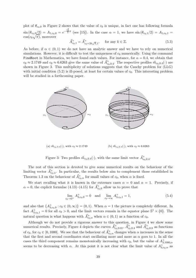
plot of θc0,0 in Figure 2 shows that the value of c0 is unique, in fact one has following formula

sin (θc0,0/2) = A1,c0,0 = e−c202π (see [15]). In the case α = 1, we have sin (θc0,1/2) = A1,c0,1 =

cos(c0√

π), moreover~A+c0,1

= ~A+c0+2k

√π,1, for any k ∈ Z. (5.3)

As before, if α ∈ (0, 1) we do not have an analytic answer and we have to rely on numericalsimulations. However, it is difficult to test the uniqueness of c0 numerically. Using the commandFindRoot in Mathematica, we have found such values. For instance, for α = 0.4, we obtain thatc0 ≈ 2.1749 and c0 ≈ 6.6263 give the same value of ~A+

c0,0.4. The respective profiles ~mc0,0.4(·) are

shown in Figure 3. This multiplicity of solutions suggests that the Cauchy problem for (LLG)with initial condition (5.2) is ill-posed, at least for certain values of c0. This interesting problemwill be studied in a forthcoming paper.

m1m2

m3

(a) ~mc0,0.4(·), with c0 ≈ 2.1749

m1m2

m3

(b) ~mc0,0.4(·), with c0 ≈ 6.6263

Figure 3: Two profiles ~mc0,0.4(·), with the same limit vector ~A+c0,0.4

.

The rest of this section is devoted to give some numerical results on the behaviour of thelimiting vector ~A+

c0,α. In particular, the results below aim to complement those established in

Theorem 1.3 on the behaviour of ~A+c0,α for small values of c0, when α is fixed.

We start recalling what it is known in the extremes cases α = 0 and α = 1. Precisely, ifα = 0, the explicit formulae (4.13)–(4.15) for ~A+

c0,0allow us to prove that

limc0→0+

A+3,c0,0

= 0 and limc0→∞

A+3,c0,1

= 1, (5.4)

and also that {A+3,c0,0

: c0 ∈ (0,∞)} = (0, 1). When α = 1 the picture is completely different. Infact A+

3,c0,1= 0 for all c0 > 0, and the limit vectors remain in the equator plane S

1 × {0}. The

natural question is what happens with ~A+c0,α when α ∈ (0, 1) as a function of c0.

Although we do not provide a rigorous answer to this question, in Figure 4 we show somenumerical results. Precisely, Figure 4 depicts the curves ~A+

c0,0.01, ~A+

c0,0.4and ~A+

c0,0.8as functions

of c0, for c0 ∈ [0, 1000]. We see that the behaviour of ~A+c0,α changes when α increases in the sense

that the first and second coordinates start oscillating more and more as α goes to 1. In all thecases the third component remains monotonically increasing with c0, but the value of A+

3,1000,α

seems to be decreasing with α. At this point it is not clear what the limit value of A+3,c0,α

as

39

c0 → ∞ is. For this reason, we perform a more detailed analysis of A+3,c0,α

and we show thecurves A+

3,1,α, A+3,10,α, A+

3,1000,α (for fixed α ∈ [0, 1]) in Figure 5. From these results we conjecturethat {A+

3,c0,·}c0>0 is a pointwise nondecreasing sequence of functions that converges to 1 for anyα < 1 as c0 → ∞. This would imply that, for α ∈ (0, 1) fixed, A1,c0,α → 0 as c0 → ∞, and sinceA1,c0,α → 1 as c0 → 0 (see (1.24)), we could conclude by continuity (see Theorem 1.3) that forany angle θ ∈ (0, π) there exists c0 > 0 such that θ is the angle between ~A+

c0,α and − ~A+c0,α (see

(5.1)). This provides an alternative way to justify the surjectivity of the map c0 7→ ~A+c0,α (in the

sense explained above).

A+1

A+2

A+3

(a) ~A+c0,0.01

A+1

A+2

A+3

(b) ~A+c0,0.4

A+1

A+2

A+3

(c) ~A+c0,0.8

Figure 4: The curves ~A+c0,0.01

, ~A+c0,0.4

and ~A+c0,0.8

as functions of c0, for c0 ∈ [0, 1000].

0

1

1α

A+3,1,α

A+3,10,α

A+3,1000,α

Figure 5: The curves A+3,1,α ,A+

3,10,α, A+3,1000,α as functions of α, for α ∈ [0, 1].

The curves in Figure 5 also allow us to discuss further the results in Theorem 1.4. In fact,when α is close to 1 the slope of the functions become unbounded and, roughly speaking, thebehaviour of A+

3,c0,αis in agreement with the result in Theorem 1.4, that is

A+3,c0,α

∼ C(c0)√1− α, as α→ 1−.

Numerically, the analysis is more difficult when α ∼ 0, because the number of computationsneeded to have an accurate profile of A+

3,c0,αincreases drastically as α → 0+. In any case,

Figure 5 suggests that A+3,c0,α

converges to A+3,c0,0

faster than√α| ln(α)|. We think that this rate

of convergence can be improved to α| ln(α)|. In fact, in the proof of Lemma 3.10 we only usedenergy estimates. Probably, taking into account the oscillations in equation (3.102) (as did inProposition 3.3), it would be possible to establish the necessary estimates to prove the followingconjecture:

| ~A+c0,α − ~A+

c0,0| ≤ C(c0)α| ln(α)|, for α ∈ (0, 1/2].

40

6 Appendix

In this appendix we show how to compute explicitly the solution ~mc0,α(s, t) of the LLG equationin the case α = 1. As a consequence, we will obtain an explicit formula for the limiting vector~A+c0,1

and the other constants appearing in the asymptotics of the associated profile establishedin Theorem 1.2 in terms of the parameter c0 in the case when α = 1.

We start by recalling that if α = 1 then β = 0. We need to find the solution {~m,~n,~b} of theSerret–Frenet system (1.6) with c(s) = c0e

−s2/4, τ ≡ 0 and the initial conditions (1.8). Hence,it is immediate that

m3 = n3 ≡ 0, b1 = b2 ≡ 0 and b3 ≡ 1.

To compute the other components, we use the Riccati equation (3.9) satisfied by the stereographicprojection of {mj , nj, bj}

ηj =nj + ibj1 +mj

, for j ∈ {1, 2}, (6.1)

found in the proof of Lemma 3.1. For the values of curvature and torsion c(s) = c0e−s2/4 and

τ(s) = 0 the Riccati equation (3.9) reads

η′j +iβs

2ηj +

c02e−αs2/4(η2j + 1) = 0. (6.2)

We see that when α = 1, and thus β = 0, (6.2) is a separable equation that we write as:

dηjη2j + 1

= −c02e−αs2/4,

so integrating, we get

ηj(s) = tan(

arctan(ηj(0)) −c02Erf(s)

)

, (6.3)

where Erf(s) is the non-normalized error function

Erf(s) =

∫ s

0e−σ2/4 dσ.

Also, using (1.8) and (6.1) we get the initial conditions η1(0) = 0 and η2(0) = 1. In particular,if c0 is small (6.3) is the global solution of the Riccati equation, but it blows-up in finite time ifc0 is large. As long as ηj is well-defined, by Lemma 3.1,

fj(s) = ec02

∫ s0e−ασ2/4ηj(σ) dσ .

The change of variablesµ = arctan(ηj(0)) −

c02Erf(s)

yields∫ s

0e−ασ2/4ηj(σ) dσ =

2

c0ln

∣

∣

∣

∣

∣

cos(

arctan(ηj(0))− c02 Erf(s)

)

cos(arctan(ηj(0)))

∣

∣

∣

∣

∣

,

and after some simplifications, we obtain

f1(s) =∣

∣

∣cos(c02Erf(s)

)∣

∣

∣and f2(s) =

∣

∣

∣cos(c02Erf(s)

)

+ sin(c02Erf(s)

)∣

∣

∣.

In view of (3.18) and (3.19), we conclude that

m1(s) = 2|f1(s)|2 − 1 = cos (c0 Erf(s)) and m2(s) = |f2(s)|2 − 1 = sin (c0 Erf(s)) . (6.4)

41

A priori, the formulae in (6.4) are valid only as long as η is well-defined, but a simple verificationshow that these are the global solutions of (1.6), with

n1(s) = − sin (c0 Erf(s)) and n2(s) = cos (c0 Erf(s)) .

In conclusion, we have proved the following:

Proposition 6.1. Let α = 1, and thus β = 0. Then, the trihedron {~mc0,1, ~nc0,1,~bc0,1} solution

of (1.6)–(1.8) is given by

~mc0,1(s) = (cos(c0 Erf(s)), sin(c0 Erf(s)), 0),

~nc0,1(s) = −(sin(c0 Erf(s)), cos(c0 Erf(s)), 0),

~bc0,1(s) = (0, 0, 1),

for all s ∈ R. In particular, the limiting vectors ~A+c0,1

and ~A−c0,1

in Theorem 1.2 are given interms of c0 as follows:

~A±c0,1

= (cos(c0√π),± sin(c0

√π), 0).

Proposition 6.1 allows us to give an alternative explicit proof of Theorem 1.2 when α = 1.

Corollary 6.2. [Explicit asymptotics when α = 1] With the same notation as in Proposition 6.1,the following asymptotics for {~mc0,1, ~nc0,1,

~bc0,1} holds true:

~mc0,1(s) =~A+c0,1

− 2c0s~B+c0,1

e−s2/4 sin(~a)− 2c20s2

~A+c0,1

e−s2/2 +O

(

e−s2/4

s3

)

,

~nc0,1(s) =~B+c0,1

sin(~a) +2c0s~A+c0,1

e−s2/4 − 2c20s2

~B+c0,1

e−s2/2 sin(~a) +O

(

e−s2/4

s3

)

,

~bc0,1(s) =~B+c0,1

cos(~a),

where the vectors ~A+c0,1

, ~B+c0,1

and ~a = (aj)3j=1 are given explicitly in terms of c0 by

~A+c0,1

= (cos(c0√π), sin(c0

√π), 0), ~B+

c0,1= (| sin(c0

√π)|, | cos(c0

√π)|, 1),

a1 =

{

3π2 , if sin(c0

√π) ≥ 0,

π2 , if sin(c0

√π) < 0,

a2 =

{

π2 , if cos(c0

√π) ≥ 0,

3π2 , if cos(c0

√π) < 0,

and a3 = 0.

Here, the bounds controlling the error terms depend on c0.

Proof. By Proposition 6.1,

~mc0,1(s) = (cos(c0√π − c0 Erfc(s)), sin(c0

√π − c0 Erfc(s)), 0),

~nc0,1(s) = −(sin(c0√π − c0 Erfc(s)), cos(c0

√π − c0 Erfc(s)), 0),

~bc0,1(s) = (0, 0, 1),

(6.5)

where the complementary error function is given by

Erfc(s) =

∫ ∞

se−σ2/4 dσ =

√π − Erf(s).

It is simple to check that

sin(c0 Erfc(s)) = e−s2/4

(

2c0s

− 4c0s3

+24c0s5

+O(c0s7

)

)

,

cos(c0 Erfc(s)) = 1 + e−s2/2

(

−2c20s2

+8c20s4

− 56c20s6

+O

(

c20s8

))

,

42

so that, using (6.5), we obtain that

m1(s) = n2(s) = cos(c0√π) +

2c0se−s2/4 sin(c0

√π)− 2c20

s2e−s2/2 cos(c0

√π) +O

(

e−s2/4

s3

)

,

m2(s) = −n1(s) = sin(c0√π)− 2c0

se−s2/4 cos(c0

√π)− 2c20

s2e−s2/2 sin(c0

√π) +O

(

e−s2/4

s3

)

.

The conclusion follows from the definitions of ~A+c0,1

, ~B+c0,1

and ~a.

Remark 6.3. Notice that ~a is not a continuous function of c0, but the vectors (B+j sin(aj))

3j=1

and (B+j cos(aj))

3j=1 are.

References

[1] M. Abramowitz and I. A. Stegun. Handbook of mathematical functions with formulas, graphs,and mathematical tables, volume 55 of National Bureau of Standards Applied MathematicsSeries. For sale by the Superintendent of Documents, U.S. Government Printing Office,Washington, D.C., 1964.

[2] V. Banica and L. Vega. On the Dirac delta as initial condition for nonlinear Schrödingerequations. Ann. Inst. H. Poincaré Anal. Non Linéaire, 25(4):697–711, 2008.

[3] H. Brézis. Opérateurs maximaux monotones et semi-groupes de contractions dans les espacesde Hilbert. North-Holland Publishing Co., Amsterdam, 1973. North-Holland MathematicsStudies, No. 5. Notas de Matemática (50).

[4] T. F. Buttke. A numerical study of superfluid turbulence in the self-induction approxima-tion. Journal of Computational Physics, 76(2):301–326, 1988.

[5] E. A. Coddington and N. Levinson. Theory of ordinary differential equations. McGraw-HillBook Company, Inc., New York-Toronto-London, 1955.

[6] M. Daniel and M. Lakshmanan. Soliton damping and energy loss in the classical continuumheisenberg spin chain. Physical Review B, 24(11):6751–6754, 1981.

[7] M. Daniel and M. Lakshmanan. Perturbation of solitons in the classical continuum isotropicHeisenberg spin system. Physica A: Statistical Mechanics and its Applications, 120(1):125–152, 1983.

[8] G. Darboux. Leçons sur la théorie générale des surfaces. I, II. Les Grands ClassiquesGauthier-Villars. [Gauthier-Villars Great Classics]. Éditions Jacques Gabay, Sceaux, 1993.Généralités. Coordonnées curvilignes. Surfaces minima. [Generalities. Curvilinear coordi-nates. Minimum surfaces], Les congruences et les équations linéaires aux dérivées partielles.Les lignes tracées sur les surfaces. [Congruences and linear partial differential equations.Lines traced on surfaces], Reprint of the second (1914) edition (I) and the second (1915)edition (II), Cours de Géométrie de la Faculté des Sciences. [Course on Geometry of theFaculty of Science].

[9] F. de la Hoz, C. J. García-Cervera, and L. Vega. A numerical study of the self-similarsolutions of the Schrödinger map. SIAM J. Appl. Math., 70(4):1047–1077, 2009.

43

[10] P. Germain and M. Rupflin. Selfsimilar expanders of the harmonic map flow. Ann. Inst. H.Poincaré Anal. Non Linéaire, 28(5):743–773, 2011.

[11] T. L. Gilbert. A lagrangian formulation of the gyromagnetic equation of the magnetizationfield. Phys. Rev., 100:1243, 1955.

[12] A. Grünrock. Bi- and trilinear Schrödinger estimates in one space dimension with applica-tions to cubic NLS and DNLS. Int. Math. Res. Not., (41):2525–2558, 2005.

[13] M. Guan, S. Gustafson, K. Kang, and T.-P. Tsai. Global questions for map evolutionequations. In Singularities in PDE and the calculus of variations, volume 44 of CRM Proc.Lecture Notes, pages 61–74. Amer. Math. Soc., Providence, RI, 2008.

[14] B. Guo and S. Ding. Landau-Lifshitz equations, volume 1 of Frontiers of Research with theChinese Academy of Sciences. World Scientific Publishing Co. Pte. Ltd., Hackensack, NJ,2008.

[15] S. Gutiérrez, J. Rivas, and L. Vega. Formation of singularities and self-similar vortex motionunder the localized induction approximation. Comm. Partial Differential Equations, 28(5-6):927–968, 2003.

[16] S. Gutiérrez and L. Vega. Self-similar solutions of the localized induction approximation:singularity formation. Nonlinearity, 17:2091–2136, 2004.

[17] P. Hartman. Ordinary differential equations. John Wiley & Sons Inc., New York, 1964.

[18] H. Hasimoto. A soliton on a vortex filament. J. Fluid Mech, 51(3):477–485, 1972.

[19] A. Hubert and R. Schäfer. Magnetic domains: the analysis of magnetic microstructures.Springer, 1998.

[20] A. M. Kosevich, B. A. Ivanov, and A. S. Kovalev. Magnetic solitons. Physics Reports,194(3-4):117–238, 1990.

[21] M. Lakshmanan. The fascinating world of the Landau-Lifshitz-Gilbert equation: anoverview. Philos. Trans. R. Soc. Lond. Ser. A Math. Phys. Eng. Sci., 369(1939):1280–1300,2011.

[22] M. Lakshmanan, T. W. Ruijgrok, and C. Thompson. On the dynamics of a continuum spinsystem. Physica A: Statistical Mechanics and its Applications, 84(3):577–590, 1976.

[23] G. L. Lamb, Jr. Elements of soliton theory. John Wiley & Sons Inc., New York, 1980. Pureand Applied Mathematics, A Wiley-Interscience Publication.

[24] L. Landau and E. Lifshitz. On the theory of the dispersion of magnetic permeability inferromagnetic bodies. Phys. Z. Sowjetunion, 8:153–169, 1935.

[25] F. Lin and C. Wang. The analysis of harmonic maps and their heat flows. World ScientificPublishing Co. Pte. Ltd., Hackensack, NJ, 2008.

[26] T. Lipniacki. Shape-preserving solutions for quantum vortex motion under localized induc-tion approximation. Phys. Fluids, 15(6):1381–1395, 2003.

[27] M. Steiner, J. Villain, and C. Windsor. Theoretical and experimental studies on one-dimensional magnetic systems. Advances in Physics, 25(2):87–209, 1976.

44

[28] D. J. Struik. Lectures on Classical Differential Geometry. Addison-Wesley Press, Inc.,Cambridge, Mass., 1950.

[29] A. Vargas and L. Vega. Global wellposedness for 1D non-linear Schrödinger equation fordata with an infinite L2 norm. J. Math. Pures Appl. (9), 80(10):1029–1044, 2001.

45