on June 17, 2018http://rspa.royalsocietypublishing.org/Downloaded from

Secondary structures in a one-dimensionalcomplex Ginzburg–Landau equation with

homogeneous boundary conditions

BY LAURENT NANA†, ALEXANDER B. EZERSKY

‡AND INNOCENT MUTABAZI*

Laboratoire Ondes et Milieux Complexes (LOMC ), FRE3102, CNRS-Universitedu Havre, 53 rue Prony, PO Box 540, 76058 Le Havre, France

Experiments in extended systems, such as the counter-rotating Couette–Taylor flow orthe Taylor–Dean flow system, have shown that patterns with vanishing amplitude mayexhibit periodic spatio-temporal defects for some range of control parameters. Theseobservations could not be interpreted by the complex Ginzburg–Landau equation(CGLE) with periodic boundary conditions. We have investigated the one-dimensionalCGLE with homogeneous boundary conditions. We found that, in the ‘Benjamin–Feirstable’ region, the basic wave train bifurcates to state with periodic spatio-temporaldefects. The numerical results match the observations quite well. We have built a newstate diagram in the parameter plane spanned by the criticality (or equivalently thelinear group velocity) and the nonlinear frequency detuning.

Keywords: pattern formation; complex Ginzburg–Landau equation; spiral vortices;periodic amplitude defects; spatio-temporal intermittency

*A†PePO‡PeCN

RecAcc

1. Introduction

Progress in the understanding of spatio-temporal dynamics of extended systemsfar from equilibrium has been achieved during the last few decades due to modelnonlinear partial differential equations (PDEs), such as the complex Ginzburg–Landau equation (CGLE) or the Kuramoto–Sivashinsky equation (Cross &Hohenberg 1993; Aranson & Kramer 2002). In many cases, for numericalsimulations of these equations, periodic boundary conditions have been used(Chate 1994; van Hecke 1998; Howard & van Hecke 2003; van Saarloos 2003).For such boundary conditions, in the case of the one-dimensional CGLEdescribing the pattern formation from Hopf bifurcation in systems withtranslational invariance, a state diagram describing the variety of regimesobserved for different parameters has been established, and the stability of thesestates has been thoroughly investigated (Brusch et al. 2000). In particular, it was

Proc. R. Soc. A (2009) 465, 2251–2265

doi:10.1098/rspa.2009.0002

Published online 29 April 2009

uthor for correspondence (mutabazi@univ-lehavre.fr).rmanent address: Departement de Physique, Faculte des Sciences, Universite de Douala,Box 24157 Douala, Cameroun.rmanent address: Laboratoire de Morphodynamique Continentale et Cotiere, UMR 6143RS-Universite de Caen-Basse Normandie, 14000 Caen, France.

eived 2 January 2009epted 1 April 2009 2251 This journal is q 2009 The Royal Society

L. Nana et al.2252

on June 17, 2018http://rspa.royalsocietypublishing.org/Downloaded from

shown that above the Benjamin–Feir (BF) line, the pattern exhibits coherentstructures, such as Nozaki–Bekki holes and spatio-temporal chaos, induced eitherby amplitude defects or phase defects (Chate 1994; Montagne et al. 1996;van Hecke 1998; Howard & van Hecke 2003). Few experiments mimicking theseconditions have been designed to validate the solutions of this equation(Kolodner et al. 1988). These systems are characterized by the translationinvariance, and the group velocity can be eliminated from the CGLE, leading thepattern to be described by a set of two control parameters (c1, c3) that will bedefined below. However, in a large number of experiments in bounded domains,patterns have a finite length and the perturbations decay near the lateral walls.This is the case, for example, in the rectangular Rayleigh–Benard convection cell(Kolodner et al. 1986); in the pattern of thermo-capillary waves in a laterallyheated liquid layer (Garnier & Chiffaudel 2001; Garnier et al. 2002); in spiralvortex flow in the Couette–Taylor flow between counter-rotating cylinders(Zaleski et al. 1985; Andereck et al. 1986; Tagg et al. 1990; Tagg 1994; Ezerskyet al. 2004); in the travelling rolls in a cylindrical annulus with a radialtemperature gradient (Lepiller et al. 2007); in the travelling inclined vortex flowin the Taylor–Dean system (Mutabazi et al. 1990; Laure & Mutabazi 1994;Bot et al. 1998; Bot & Mutabazi 2000); and in parametrically excited ripples inviscous fluids (Ezersky et al. 2001). To explain the regimes observed in theseexperiments on pattern formation in bounded flow systems with lateralboundaries, it is necessary to consider the conditions that are more close toexperimental situations. The boundary conditions have an influence on thestability of the system and pattern generation. In fact, different results have beenfound from numerical resolution of the CGLE for the complex amplitude A(x,t)in systems with a finite length L by using various types of boundary conditions.Deissler (1985) has used the boundary conditions Axx(0,t)Z0 to mimic an openflow at the inlet xZ0 and A(L,t)Z0 for the outlet. Tobias & Knobloch (1998)have used the boundary conditions A(0,t)ZA(L,t)Z0 to illustrate the variety ofnovel behaviours that occur when unidirectional waves interact with boundaries:wall mode and front between patterns emerging from destabilization of the wavetrain. Tobias et al. (1998) have used the conditions Ax(0,t)ZA(L,t)Z0 to studythe problem of breakup of spiral waves into chemical turbulence in which xZ0plays the role of the core and xZL the outer boundary. Lucke & Recktenwald(1993) have investigated the pattern growth resulting from an inlet boundarycondition that is produced by thermal equilibrium transverse momentumfluctuations that are advected into the system at xZ0. The influence ofboundary conditions was also highlighted recently for a two-dimensional CGLE(Eguiluz et al. 1999, 2000, 2001). It was shown that homogeneous Dirichletboundary conditions induce a strong selection mechanism of pattern wavenumberand frequency because of the absorption of disturbances on the lateral edges.

The present work deals with one-dimensional patterns described by the CGLEin finite geometry in which the amplitude of the supercritical wave patternvanishes at the lateral boundaries of the domain. We will show numerically that,due to the group velocity, the state diagram differs fundamentally from thatobtained for periodic boundary conditions (Chate 1994; Montagne et al. 1996;van Hecke 1998; Brusch et al. 2000; Howard & van Hecke 2003; van Saarloos2003). A sequence of periodic defects (PDs) in the BF stable region will beexcited in a finite zone of the parameter space.

Proc. R. Soc. A (2009)

2253Complex Ginzburg–Landau equation

on June 17, 2018http://rspa.royalsocietypublishing.org/Downloaded from

The paper is organized as follows: in the second section, we present theamplitude equation and the numerical algorithm; in §3, we present the resultsthat will be discussed in §4; and §5 is devoted to the conclusion of the study.

2. Amplitude equation and numerical scheme

Different physical and chemical systems driven out of equilibrium may undergoHopf bifurcations leading to a rich variety of spatio-temporal behaviours. In mostcases, these bifurcations occur with broken spatial and temporal symmetries andthey induce the formation of wave patterns that are described by an orderparameter A(x,t), such that AZ0 in the high symmetry state and As0 in thelow symmetry state. The field of the wave pattern is given by Cross & Hohenberg(1993) and Aranson & Kramer (2002),

uðx; rt; tÞZAðx; tÞeiðkcxCuctÞuðrtÞCc:c:; ð2:1Þwhere the parameter order A(x,t) is a complex amplitude (AZjAjeif) of the slowdynamics of the waves; c.c. stands for the complex conjugate; and theeigenfunction uðrtÞdepends on the coordinates rt perpendicular to the criticalwavevector. When both the critical wavenumber kc and frequency uc are non-zero at the pattern forming Hopf bifurcation, the primary modes are travellingwave dynamics, which can be described by the CGLE for the complex amplitude(Bot et al. 1998; Bot & Mutabazi 2000). In a one-dimensional system, it is usuallywritten as

vA

vtKs

vA

vxZmACð1C ic1Þ

v2A

vx2Kð1K ic3Þ jA j 2A; 0%x%L; ð2:2Þ

where s is the linear group velocity of a left travelling wave (for sO0); m isthe relative distance of the control parameter from the critical point; and thecoefficients c1 and c3 describe linear dispersion and nonlinear frequency detuning,respectively. The parameters m and s act together by means of the scaled group

velocity, VgZs=ffiffiffiffiffiffiffiffiffiffiffiffiffiffiffiffiffiffiffimð1Cc21Þ

p. In this work, we have imposed on the complex

amplitude the following boundary conditions:

Aðx Z 0; tÞZ 0ZAðx ZL; tÞ: ð2:3ÞThese boundary conditions are realized in different extended systems, where thepattern amplitude vanishes near lateral boundaries (Zaleski et al. 1985; Anderecket al. 1986; Mutabazi et al. 1990; Tagg et al. 1990; Laure & Mutabazi 1994; Tagg1994; Bot et al. 1998; Bot & Mutabazi 2000; Ezersky et al. 2001, 2004; Garnier &Chiffaudel 2001; Garnier et al. 2002; Lepiller et al. 2007). Contrary to theproblem with periodic boundary conditions, the group velocity s cannot beremoved from the equation since the system has no Galilean invariance.Therefore, the present formulation introduces the linear group velocity as a newparameter. The length L of the system is fixed in the experiment, while it takesdiscrete values for periodic boundary conditions. Therefore, in one-dimensionalsystems with a finite length, the CGLE is spanned by a space of three controlparameters, (s, c1, c3) while it is spanned by only two control parameters (c1, c3)in the case of an extended system. For convenience, we have chosen to fix the

Proc. R. Soc. A (2009)

L. Nana et al.2254

on June 17, 2018http://rspa.royalsocietypublishing.org/Downloaded from

linear group velocity s and to vary the criticality parameter m, which is moreaccessible in experiment than the linear group velocity. In the discussion, we willpresent the scaled CGLE where the parameter m has been removed.

The numerical method used throughout is the finite-difference scheme in spaceand the fourth-order Runge–Kutta algorithm in time. In fact, the finite-differencescheme allows the discrete form of the CGLE (equation (2.2)) to be obtained.Such a discretization scheme of this equation has been used in different works, forexample, for description of vortex line dynamics (Willaime et al. 1991) or for thedetermination of coefficients of the Ginzburg–Landau equation from experi-mental spatio-temporal data in the wakes behind an array of cylinders (Le Galet al. 2003). In these two examples, the oscillation of each isolated cell (eachvortex or each wake) obeys a complex Landau equation which is the normal formof the Hopf bifurcation that gives rise to each oscillator. The global behaviour ofthe vortex or the wake arrays was described by the dynamics of coupled Hopfoscillators. Ravoux et al. (2000) analysed the stability of the nonlinear planewave solutions of the discretized CGLE. The discretized CGLE reads

dAj

dtZmAjKð1K ic3Þ jAj j 2Aj Cs

AjC1KAjK1

2DxCð1C ic1Þ

AjC1K2Aj CAjK1

ðDxÞ2;

ð2:4aÞ

where AjZAðxj ; tÞ, with 2%j%NK1, and the homogeneous boundary conditions

(equation (2.3)) were

A1 ZAN Z 0: ð2:4bÞ

Thus, we have reduced the PDE to a system of ordinary differential equations.The structure of such systems implies that their dynamics is the result ofinteraction between N individual dynamical entities. We have integratednumerically the system (2.4a) and (2.4b) using a standard fourth-order Runge–Kutta method. In our numerical simulations, we have considered a systeminvolving N sites with NZ301. The accuracy of the numerical procedure has beenexamined by testing different time and space steps. The time step must be smallenough at a given spacing to ensure the conditional stability of the precedingalgorithm at each step. Finally, the time and space increments were chosen to beDtZ0.025 and DxZ0.2. We have chosen as initial condition a symmetric centredpulse-like solution given by

Aðxj ; 0ÞZA0ð1C iÞ=coshðgðxjK xaÞÞ; with xj Z ð jK1ÞDx and 1! j!N ;

ð2:5Þ

where A0 and g are constants and xaZL/2 is the position of the maximum of thisinitial perturbation. Since the initial perturbation must satisfy the boundaryconditions (2.4b), A0 must be a small quantity and g a large one. That is why,in our numerical calculations, we have chosen A0Z0.01 and gZ100. Thus,depending on the nature of the nonlinear dynamics of the system, the initialdisturbance can grow and invade the domain (global mode) or it can be expelledfrom the system (convective instability).

Proc. R. Soc. A (2009)

60

50

40

30

fron

t pos

ition

20

10

0100 150 250200 300 350

time, t400 450 500

7

6

5

4

(a)

(c)

(b)

3

2

1

0 10 20 30 40 50 60

0.30

0.25

0.20

0.15

0.10

0.05

0 10 20 30 40 50 60

Figure 1. Profiles of the amplitude of an initial perturbation at different times for sZ0.50,c1Zc3Z0.50 and LZ60: (a) in the convective instability regime (mZ0.045); (b) in the global moderegime (mZ0.065); and (c) is the variation of the front position for mZ0.065.

2255Complex Ginzburg–Landau equation

on June 17, 2018http://rspa.royalsocietypublishing.org/Downloaded from

3. Results of numerical simulations

The control parameters c1, s and L were fixed at c1Z0.50, sZ0.50 and LZ60,and we have varied m and c3. This variation enabled us to identify, in theparameter space (m, c3), zones in which the patterns exhibit different behaviours.

A linear growth analysis of the CGLE (2.2) in unbounded domains alongthe lines of Cross & Hohenberg (1993) shows that the far front separating thebase state (AZ0) and the bifurcated state (As0) moves with velocityV fZ2ð1C c21Þ1=2Ks. In the convectively unstable region 0!m!ma, the frontpropagates upstream so that Vf!0, the scaled group velocity VgO2 and theamplitude of the pattern decays locally (figure 1a). In the absolutely unstableregime, mOma, it moves downstream, i.e. VfO0, the scaled group velocity Vg!2and the bifurcated state (global mode) invades the whole system (figure 1b). Atthe boundary mZma, the front is stationary and the scaled group velocity VgZ2.To validate our numerical scheme, we have retrieved the analytical results forabsolute and convective instability for our parameters s, c1 and L. For the chosenvalues of these parameters, the transition between convective instability and

Proc. R. Soc. A (2009)

4

3

2

1

0

–1

–2

–3

–4

–50 0.05 0.10 0.15 0.20 0.25 0.30 0.35 0.40 0.45 0.50 0.55

PD

global mode

global mode

secondary instability

secondary instability

Figure 2. States diagram in the parameter plane (m, c3) obtained from numerical solution of theCGLE (equation (2.2)) for c1Z0.50, sZ0.50 and LZ60. PD stands for periodic defects region.

L. Nana et al.2256

on June 17, 2018http://rspa.royalsocietypublishing.org/Downloaded from

absolute instability occurs at mabsZ0.05, i.e. VfZ0 (Tobias et al. 1998).Moreover, for mZ0.065, the velocity of the front propagation found numericallyis Vfz0.08 for LZ60 (figure 1c), which is in a good agreement with the analyticalVfz0.07 in the limit L/N. With increasing m, the nonlinear wave trainbroadens out to a larger value of x, until it fills the entire domain.

Our goal was to investigate the effects of the nonlinear dispersion coefficient c3of the CGLE on the dynamics of the system, with the prescribed boundaryconditions (2.3). Solving the CGLE for several values of c3, we found that, inthe convective instability regime, the system is practically insensitive to thevariation of the coefficient of the nonlinear dispersion. In the absolute instabilityregime (i.e. for mR0.05), the variation of the coefficient c3 leads to bifurcationof the global mode to new states that are summarized in the state diagram offigure 2 for c32[K5;5]. The global mode is stable between lines L3KL2 and L1.Above the line L1 and below the line L2, the global mode pertains to a secondaryinstability that leads to different types of pattern, depending on the sign of c3 andthe value of m.

The space–time diagram of the phase of the global mode near the line L1

(figure 3) shows that the pattern propagates in only one direction, with anaverage frequency uZ0.06 and wavenumber kZ0.30. The behaviour of theglobal mode above the line L1 is represented by figure 4 for mZ0.15 and c3Z3.65.The regular pattern is destabilized and gives rise to a modulated state in spaceand time near the wall xZ0, while, near the end xZL, the pattern remains non-modulated. We therefore have obtained a state with two patterns separatedby a front at the position x f. Figure 4a,b shows a regular wave train in x f!x!Land a modulated pattern in 0!x!x f, with wavenumber kmz1.07 and frequencyumz1.40. The front position moves in time with the group velocity s. It movestowards the wall xZL with increasing c3.

Proc. R. Soc. A (2009)

01000

0

950900850800750700650600550

10 20 30 40 50 60 10 20 30 40 50 60

0.6 0.7

0.6

0.5

0.4

0.3

0.2

0.1

0.5

0.4

0.3

0.2

0.1

(a) (b)

Figure 4. Space–time variation of the amplitude modulus jAj showing the appearance ofthe secondary structures; one can observe the amplitude modulation of the global mode. Theparameter values are c1Z0.50, c3Z3.65, sZ0.50, mZ0.15 and LZ60.

10000 10 20 30 40 50 60

–3

–2

–1

0

1

2

3

900

800

700

600

500

400

300

200

Figure 3. Space–time variation of the global mode phase for mZ0.15, sZ0.50, c1Z0.50, c3Z3.00and LZ60.

2257Complex Ginzburg–Landau equation

on June 17, 2018http://rspa.royalsocietypublishing.org/Downloaded from

For negative values of c3, the global mode is destabilized differently. In theparameter region between L3 and L4, the global mode exhibits amplitude defects:points in the space–time diagram where the amplitude of the wave vanishes(jAjz0) and the phase (fZarg(A)) is not defined (figure 5). These amplitudedefects appear at regular time intervals; for this reason we have called themtime-PDs, and the frequency of their appearance increases with increasing valuesof m and c3. On the space–time diagram of figure 5a, one observes a sequence offour-point defects on an interval of time tz100. The slope of the defects observedin figure 5a indicates the direction of wave propagation.

Proc. R. Soc. A (2009)

830(a)

(c)

(b)0.35

0.30

0.25

0.20

0.15

0.10

0.05

840850860870880890900910920930

0 10 20 30 40 50 60

830840850860870880890900910920930

3

2

1

0

–1

–2

–30 10 20 30 40 50 60

830840850860870880890900910920930

3

2

1

0

–1

–2

–30 10 20 30 40 50 60

a

Figure 5. Spatio-temporal diagram of: (a) amplitude of the pattern showing a sequence of four time-PDs, grey level range from black (0) to white (the maximum); (b) the phase arg(u(x,t)) of thepattern field is mapped to grey scale (black, Kp/white, Cp), a jump of p is observed around adefect; and (c) the phase perturbation, in the core of the defect, a 2p phase shift is accumulatedaround the circular arc shown. The parameters are c1Z0.50, c3ZK4.30, sZ0.50, mZ0.15 and LZ60.

L. Nana et al.2258

on June 17, 2018http://rspa.royalsocietypublishing.org/Downloaded from

In order to characterize these amplitude defects, we have computed thehydrodynamic field u(x, t) defining the wave packet in the simplest form,

uðx; tÞZAðx; tÞexp½iðu0tCk0xÞ�Cc:c:; ð3:1Þwhere c.c. stands for the complex conjugate term. In our numerical simulations,we have fixed u0Z1.5 and k0Z2.0, taken from the experimental data of theCouette–Taylor flow (Ezersky et al. 2004). The space–time diagram of figure 5bshows the grey level of the phase of the field u(x,t). The phase varies from Kp(black) to Cp (white) and undergoes a jump of p in the position of the core of adefect. The space–time diagram of figure 5c is that of the phase perturbationobtained after a complex demodulation. The amplitude profile of the global modein the neighbourhood of a single defect is shown in figure 6a. The core of thedefect is located at xdz15. Figure 6b illustrates the temporal evolution ofthe mode amplitude along the four defects.

In the vicinity of an isolated defect, levels of constant amplitude are ellipsesstretched along one direction. Figure 7a shows the defect situated at the positionðxd; tdÞzð15; 866Þ. The angle of inclination of each ellipse is approximately the

Proc. R. Soc. A (2009)

853

855

860

865

870

87513 14 15 16 17 18

863

868

878 0.260.26

0.260.260.230.23 0.250.25

0.20.20.170.17

0.110.110.080.08 0.060.06

0.14

0.14

0.2 0.23

0.23

0.170.2

0.14

0.08

0.06

0.110.03

0.03

0.060.060.11

0.14

0.170.17

0.2

0.2

0.23

0.250.28

0.28 0.250.250.23

0.110.14

0.080.08

0.25

0.170.170.140.14

12.5 15.5

855

860

865

870

87513 14 15 16 17 18

18.5

8533

2

1

0

–1

–2

–3

863

868

87812.5 15.5 18.5

0.280.28

0.110.11

0.140.14

0.17

0.25

0.23

0.20.17

0.110.14

0.260.26

0.260.260.230.23 0.250.25

0.20.20.170.17

0.110.110.080.08 0.060.06

0.14

0.14

0.2 0.23

0.23

0.170.2

0.14

0.08

0.06

0.110.03

0.03

0.060.060.11

0.14

0.170.17

0.2

0.2

0.23

0.250.28

0.28 0.250.250.23

0.110.14

0.080.08

0.25

0.170.170.140.14

0.280.28

0.110.11

0.140.14

0.17

0.25

0.23

0.20.17

0.110.14

0.260.260.260.280.280.28

0.260.23 0.25

0.250.250.250.250.25

0.20.17

0.110.08 0.06

0.14

0.2 0.23

0.23

0.170.2

0.14

0.08

0.06

0.110.03

0.03

0.060.060.11

0.14

0.17

0.2

0.2

0.23

0.250.28

0.28 0.250.23

0.110.14

0.08

0.25

0.170.14

0.28

0.11

0.14

0.17

0.25

0.23

0.20.17

0.110.14

(a) (b)

(c) (d)

Figure 7. (a) Levels of constant amplitude jAj; (b) the phase arg(A) of the pattern in the vicinity ofan isolated point defect, obtained by numerical simulations of equation (2.2); and (c,d ) iso-amplitude lines obtained from our approximate solution (equation (3.2)), with bZ0.30 for twovalues of the linear group velocity sZ0.50 and 0.20, respectively.

0.35 (a) (b)

0.30

0.25

0.20

0.15

0.10

0.05

0 10 20 30 40 50 60 820 840 860 880 900 920 940

Figure 6. (a) Spatial profile and (b) temporal evolution of the pattern amplitude in theneighbourhood of the defect core located at xdZ15. t1Z839, t2Z866, t3Z893 and t4Z920 andthe time period is TZt2Kt1Zt3Kt2Zt4Kt3Z27, where t1, t2, t3 and t4 represent the instants ofappearance of the four chosen defects of figure 5a.

2259Complex Ginzburg–Landau equation

Proc. R. Soc. A (2009)

on June 17, 2018http://rspa.royalsocietypublishing.org/Downloaded from

830(a) (b)

0.35

0.30

0.25

0.20

0.15

0.10

0.05

840850860870880890900910920930

0 10 20 30 40 50 60

830840850860870880890900910920930

3

2

1

0

–1

–2

–30 10 20 30 40 50 60

a

Figure 8. Space–time diagram of (a) the modulus jAj of the amplitude of the wave and (b) the phasearg(u(x,t)) of the pattern field, showing a sequence of topological defects. Amplitude holes maydevelop away from some defects. The equation parameters are c1Z0.50, c3ZK5.00, sZ0.50 andmZ0.18.

L. Nana et al.2260

on June 17, 2018http://rspa.royalsocietypublishing.org/Downloaded from

same for all point defects. We have verified that the inclination of the ellipse isdetermined by the group velocity of the wave pattern. For example, theinclination of the ellipse axis in figure 7a is 0.6, while the group velocity ofperturbations is sZ0.5. It should be emphasized that, unlike Nozaki–Bekki holeswhich move with definite velocity, amplitude defects exist in the space–timediagram at a definite time and coordinate. Nevertheless, the group velocity of thepatterns is displayed by the distribution of amplitude and phase in the vicinity ofthe defect. The phase of the wave pattern in the vicinity of the point defect isshown in figure 7b, and the clockwise circulation of the gradient phase around thispoint is FV½argðAÞ�dlZ2p. In the vicinity of an isolated defect, the amplitude andphase fields can be represented by a simple model of complex amplitude,

Aðc; tÞZ ð1C ibÞcCst; ð3:2Þ

where cZxKxd; tZtKtd; and b is an ad hoc parameter. It is possible to check thatsuch a function is a solution of equation (2.2). The levels of constant amplitude

Aðc; tÞj jZffiffiffiffiffiffiffiffiffiffiffiffiffiffiffiffiffiffiffiffiffiffiffiffiffiffiffiffiffiffiffiffiffiffiffiffiðbcÞ2CðcCstÞ2

pand constant phase Fðc; tÞZtanK1 ½bc=ðcCstÞ�

are topologically similar to those obtained numerically in the vicinity of the defects.The similarity includes the inclination of ellipses (lines of constant amplitude infigure 7c,d ), which are related to the group velocity.

The position of the defects in the pattern depends on the values of the controlparameters (m, c3). For small values of m, defects appear in the vicinity of thewall (xZ0). When the parameters m and c3 are increased, defects move towardsthe interior of the domain. Figure 8a presents the space–time diagram of theamplitude of the wave pattern in the zone between the lines L2 and L4 in figure 2.We have selected the values of parameters m and c3 close to the line L4. Thesequence of PDs appears now in the middle of the domain and travelling holes-like solutions are observed near the wall xZ0. Figure 8b is the space–timediagram of the phase of the constructed pattern field. When one moves awayfrom the line L4, the behaviour of the pattern becomes more complex withirregular distribution of a large number of holes and amplitude defects.

Proc. R. Soc. A (2009)

2261Complex Ginzburg–Landau equation

on June 17, 2018http://rspa.royalsocietypublishing.org/Downloaded from

4. Discussion

In the simulations of the CGLEs with homogeneous boundary conditions, wehave found new states that were different from those previously obtained bymany authors that used periodic boundary conditions (Chate 1994; Montagneet al. 1996; van Hecke 1998; Brusch et al. 2000; Howard & van Hecke 2003;van Saarloos 2003) or homogeneous boundary conditions (Tobias et al. 1998).The importance of boundary conditions on solutions of a PDE is a well-knownproperty (Tikhonov & Samarskii 1990). Tobias & Knobloch (1998), Tobias et al.(1998) and Eguiluz et al. (1999, 2000, 2001) have shown that homogeneousboundary conditions may change significantly the pattern generated in thesystem. In the case of positive values of c3, we have found states (figures 3 and 4)that are similar to those obtained by Tobias et al. (1998). These authors haveinvestigated thoroughly the stability of the obtained states, and have shown thatthe transition is ruled by the change of the nature of the instability of the basicwave train from convective to absolute secondary instability. For negative valuesof c3 (the BF stable region), we have found new patterns that exhibited temporalperiodic amplitude defects with or without travelling holes, depending on thevalues of c3. The stability analysis of the basic wave train for c3!0 is beyondthe scope of the present work. To our best knowledge, these states were notreported in numerical simulations. In fact, many previous studies (Chate 1994;Montagne et al. 1996; van Hecke 1998; Brusch et al. 2000; Howard & van Hecke2003; van Saarloos 2003) of the CGLE with periodic boundary conditionsreported amplitude defect generation in the region of BF instability, i.e. when1Kc1c3!0. In our case, since we have fixed c1Z0.5, the BF unstable zonecorresponds to the region with c3O2 (figure 2). Temporal periodic amplitudedefects were obtained for c3!0. Such defects have been observed in the spiralpattern in the counter-rotating Couette–Taylor system (Ezersky et al. 2004), inthe travelling roll pattern in the cylindrical annulus with a radial temperaturegradient (Lepiller et al. 2007), in the Taylor–Dean system (Mutabazi et al.1990; Bot et al. 1998; Bot & Mutabazi 2000) or in binary mixture convection(Voss et al. 1999). Appearance of periodic sequences of point defects in spatio-temporal diagrams seems to be typical for the systems with rotation symmetry(Ostrovsky & Potapov 1999). Numerical simulations of the anisotropic CGLEhave presented a class of solutions where the defects were aligned spontaneouslyalong chains (Weber et al. 1991). These chains, which bear some resemblancewith chevron patterns, have been observed in liquid crystal convection(Rossberg & Kramer 1998) and have been discussed in more detail by Weberet al. (1992) and Faller & Kramer (1999).

We should emphasize that periodic amplitude defects can be obtained only forhomogeneous boundary conditions, and cannot be found for periodic boundaryconditions. This may be explained as follows: for solutions with defects, the phaseof the complex amplitude A(x, t) at a given time t is not periodic and

fðLÞKfð0Þs0; G2p;G4p;G6p;.:

It is impossible to glue this solution at the ends in order to satisfy periodicboundary conditions. The length L of the domain plays a crucial role in ourstudy. We have varied the length L and found that the observed secondary

Proc. R. Soc. A (2009)

4

5

3

2

1

0

–1

–2

–3

–4

–50 0.2 0.4 0.6 0.8 1.0 1.2 1.4 1.6 1.8 2.0

L3

L4

L2

L1

PD

global mode

global mode

secondary instability

secondary instability

Figure 9. State diagram in the parameter plane (V,c3) obtained from numerical solution of theCGLE (equation (4.1)) for a system length lZ600. (CC) is the region of the parameter plane wherethe spatio-temporal intermittency is observed.

L. Nana et al.2262

on June 17, 2018http://rspa.royalsocietypublishing.org/Downloaded from

structures appeared at positions x f or xd, which increases with the length L. Theposition of the defects in the pattern depends on the values of the controlparameters (m, c3), but also on the initial conditions; for different initialconditions, PDs appeared at different coordinates xd.

In order to exclude the influence of the parameter m and for a bettercomparison with previous results, we have solved the CGLE in the scaled form

vA

vTKV

vA

vXZACð1C ic1Þ

v2A

vX2Kð1K ic3Þ jA j2A; 0%X% l; ð4:1Þ

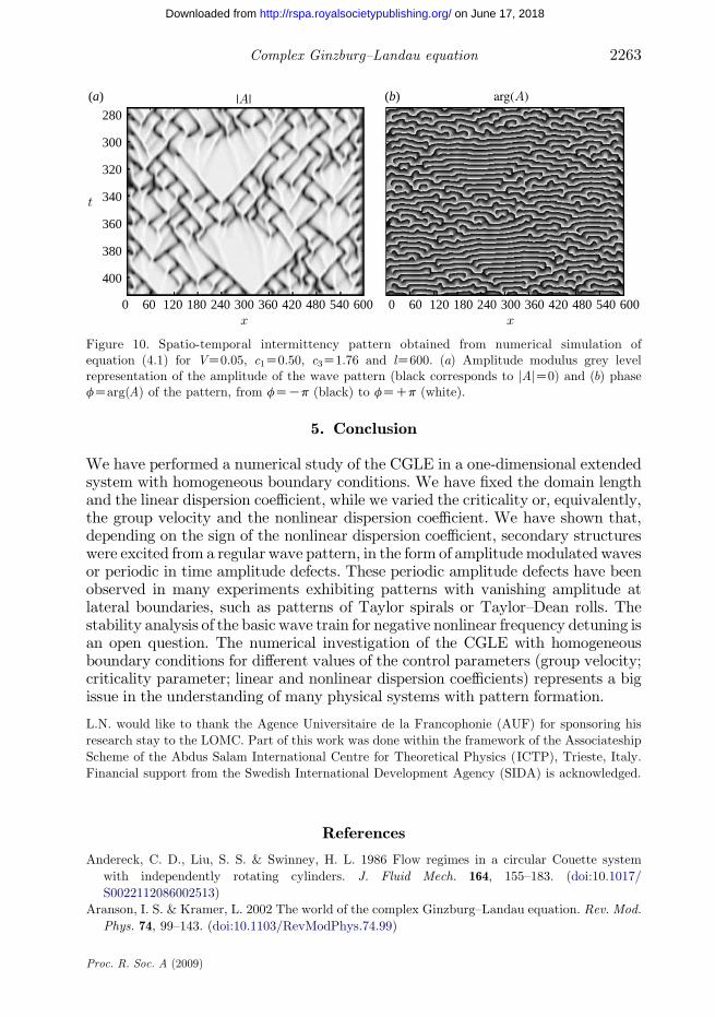
where we have introduced the scaled coordinate XZm1/2x and time TZmt. Thenew scaled group velocity VZsmK1/2 and the domain length becomes lZm1/2L.The corresponding state diagram has been plotted in figure 9 in the parameterplane (V,c3) for lZ600. One can observe that the state diagram in theparameter plane (V,c3) of equation (4.1) is almost equivalent to that inthe parameter plane (m, c3) of equation (2.2) presented in figure 2. The differenceoccurs for small values of the linear group velocity (V/0). When the linear groupvelocity vanishes (VZ0) and c1Z0.50 and c3Z1.76, we retrieved the spatio-temporal intermittency of van Hecke (1998). We have plotted in figure 10a thecharacteristic pattern of a spatio-temporal intermittent regime for VZ0.05, inwhich a global mode coexists with a chaotic attractor: the state consists of patchesof plane waves, separated by various holes, i.e. local structures characterized bydepression of the amplitude jAj of the pattern. Similar patterns called ‘hole-defectchaos’ were obtained in simulations of equation (4.1) with periodic boundaryconditions (Howard & van Hecke 2003) for parameters c1Z0.6, c3Z1.4 andlZ500. Our simulations show that, for a small group velocity, homogeneousboundary conditions only slightly modify the region of ‘hole-defect chaos’.

Proc. R. Soc. A (2009)

0

400

380

360

340

320

300

280

60 120 180 240 300 360 420 480 540 600 0 60 120 180 240 300 360 420 480 540 600

(a) (b)

Figure 10. Spatio-temporal intermittency pattern obtained from numerical simulation ofequation (4.1) for VZ0.05, c1Z0.50, c3Z1.76 and lZ600. (a) Amplitude modulus grey levelrepresentation of the amplitude of the wave pattern (black corresponds to jAjZ0) and (b) phasefZarg(A) of the pattern, from fZKp (black) to fZCp (white).

2263Complex Ginzburg–Landau equation

on June 17, 2018http://rspa.royalsocietypublishing.org/Downloaded from

5. Conclusion

We have performed a numerical study of the CGLE in a one-dimensional extendedsystem with homogeneous boundary conditions. We have fixed the domain lengthand the linear dispersion coefficient, while we varied the criticality or, equivalently,the group velocity and the nonlinear dispersion coefficient. We have shown that,depending on the sign of the nonlinear dispersion coefficient, secondary structureswere excited from a regular wave pattern, in the form of amplitudemodulated wavesor periodic in time amplitude defects. These periodic amplitude defects have beenobserved in many experiments exhibiting patterns with vanishing amplitude atlateral boundaries, such as patterns of Taylor spirals or Taylor–Dean rolls. Thestability analysis of the basic wave train for negative nonlinear frequency detuning isan open question. The numerical investigation of the CGLE with homogeneousboundary conditions for different values of the control parameters (group velocity;criticality parameter; linear and nonlinear dispersion coefficients) represents a bigissue in the understanding of many physical systems with pattern formation.

L.N. would like to thank the Agence Universitaire de la Francophonie (AUF) for sponsoring his

research stay to the LOMC. Part of this work was done within the framework of the Associateship

Scheme of the Abdus Salam International Centre for Theoretical Physics (ICTP), Trieste, Italy.

Financial support from the Swedish International Development Agency (SIDA) is acknowledged.

References

Andereck, C. D., Liu, S. S. & Swinney, H. L. 1986 Flow regimes in a circular Couette system

with independently rotating cylinders. J. Fluid Mech. 164, 155–183. (doi:10.1017/

S0022112086002513)

Aranson, I. S. & Kramer, L. 2002 The world of the complex Ginzburg–Landau equation. Rev. Mod.

Phys. 74, 99–143. (doi:10.1103/RevModPhys.74.99)

Proc. R. Soc. A (2009)

L. Nana et al.2264

on June 17, 2018http://rspa.royalsocietypublishing.org/Downloaded from

Bot, P. & Mutabazi, I. 2000 Dynamics of spatio-temporal defects in the Taylor–Dean system. Eur.

Phys. J. B 13, 141–155.Bot, P., Cadot, O. & Mutabazi, I. 1998 Secondary instability mode of a roll pattern and transition

to spatiotemporal chaos in the Taylor–Dean system. Phys. Rev. E 58, 3089–3097. (doi:10.1103/PhysRevE.58.3089)

Brusch, L., Zimmermann, M. G., van Hecke, M., Bar, M. & Torcini, A. 2000 Modulated amplitude

waves and the transition from phase to defect chaos. Phys. Rev. Lett. 85, 86–89. (doi:10.1103/PhysRevLett.85.86)

Chate, H. 1994 Spatiotemporal intermittency regimes of the one-dimensional complex Ginzburg–Landau equation. Nonlinearity 7, 185–204. (doi:10.1088/0951-7715/7/1/007)

Cross, M. C. & Hohenberg, P. C. 1993 Pattern formation outside of equilibrium. Rev. Mod. Phys.65, 851–1112. (doi:10.1103/RevModPhys.65.851)

Deissler, R. J. 1985 Noise-sustained structure, intermittency, and the Ginzburg–Landau equation.J. Stat. Phys. 40, 371–395. (doi:10.1007/BF01017180)

Eguiluz, V. M., Hernandez-Garcia, E. & Piro, O. 1999 Boundary effects in the complex Ginzburg–Landau equation. Int. J. Bif. Chaos 9, 2209–2214. (doi:10.1142/S0218127499001644)

Eguiluz, V. M., Hernandez-Garcia, E. & Piro, O. 2000 Boundary effects in extended dynamical

systems. Physica A 283, 48–51. (doi:10.1016/S0378-4371(00)00126-6)Eguiluz, V. M., Hernandez-Garcia, E. & Piro, O. 2001 Complex Ginzburg–Landau equation in the

presence of walls and corners. Phys. Rev. E 64, 036 205. (doi:10.1103/PhysRevE.64.036205)Ezersky, A. B., Kiyashko, S. V. & Nazarovsky, A. V. 2001 Bound states of topological defects

in parametrically excited capillary ripples. Physica D 152, 310–324. (doi:10.1016/S0167-2789(01)00176-2)

Ezersky, A. B., Latrache, N., Crumeyrolle, O. & Mutabazi, I. 2004 Competition of spiral waveswith anomalous dispersion in Couette–Taylor flow. Theor. Comput. Fluid Dyn. 18, 85–95.

(doi:10.1007/s00162-004-0139-z)Faller, R. & Kramer, L. 1999 Phase chaos in the anisotropic complex Ginzburg–Landau equation.

Chaos Solitons Fractals 10, 745–752. (doi:10.1016/S0960-0779(98)00024-1)Garnier, N. & Chiffaudel, A. 2001 Nonlinear transition to a global mode for traveling-wave

instability in a finite box. Phys. Rev. Lett. 86, 75–78. (doi:10.1103/PhysRevLett.86.75)Garnier, N., Chiffaudel, A. & Daviaud, F. 2002 Convective and absolute Eckhaus instability

leading to modulated waves in a finite box. Phys. Rev. Lett. 88, 134 501. (doi:10.1103/

PhysRevLett.88.134501)Howard, M. & van Hecke, M. 2003 Hole-defect chaos in the one-dimensional complex Ginzburg–

Landau equation. Phys. Rev. E 68, 026 213. (doi:10.1103/PhysRevE.68.026213)Kolodner, P., Walder, R. W., Passner, A. & Surko, C. M. 1986 Rayleigh–Benard convection in an

intermediate-aspect-ratio rectangular container. J. Fluid Mech. 163, 195–226. (doi:10.1017/S0022112086002276)

Kolodner, P., Bensimon, D. & Surko, C. M. 1988 Traveling-wave convection in an annulus. Phys.Rev. Lett. 60, 1723–1726. (doi:10.1103/PhysRevLett.60.1723)

Laure, P. & Mutabazi, I. 1994 Nonlinear analysis of instability modes in the Taylor–Dean system.

Phys. Fluids 6, 3630. (doi:10.1063/1.868420)Le Gal, P., Ravoux, J. F., Floriani, E. & Dudok de Wit, T. 2003 Recovering the coefficients of the

complex Ginzburg–Landau equation from experimental spatio-temporal data: two examplesfrom hydrodynamics. Physica D 174, 114–133. (doi:10.1016/S0167-2789(02)00686-3)

Lepiller, V., Prigent, A., Dumouchel, F. & Mutabazi, I. 2007 Transition to turbulence in a tallannulus submitted to a radial temperature gradient. Phys. Fluids 19, 054 101. (doi:10.1063/

1.2721756)Lucke, M. &Recktenwald, A. 1993 Amplification of molecular fluctuations into macroscopic vortices

by convective instabilities. Europhys. Lett. 22, 559–564. (doi:10.1209/0295-5075/22/8/001)Montagne, R., Hernandez-Garcia, E. & San Miguel, M. 1996 Winding number instability in the

phase-turbulence regime of the complex Ginzburg–Landau equation. Phys. Rev. Lett. 77,267–270. (doi:10.1103/PhysRevLett.77.267)

Proc. R. Soc. A (2009)

2265Complex Ginzburg–Landau equation

on June 17, 2018http://rspa.royalsocietypublishing.org/Downloaded from

Mutabazi, I., Hegseth, J. J., Andereck, C. D. & Wesfreid, J. E. 1990 Spatiotemporal patternmodulations in the Taylor–Dean system. Phys. Rev. Lett. 64, 1729–1732. (doi:10.1103/PhysRevLett.64.1729)

Ostrovsky, L. A. & Potapov, A. I. 1999 Modulated waves. Theory and applications. Baltimore, MD:The John Hopkins University Press.

Ravoux, J. F., Le Dizes, S. & Le Gal, P. 2000 Stability analysis of plane wave solutions of thediscrete Ginzburg–Landau equation. Phys. Rev. E 61, 390–393. (doi:10.1103/PhysRevE.61.390)

Rossberg, A. G. & Kramer, L. 1998 Pattern formation from defect chaos—a theory of chevrons.Physica D 115, 19–28. (doi:10.1016/S0167-2789(97)00223-6)

Tagg, R. 1994 The Couette–Taylor problem. Non. Sci. Today 4, 1–25.Tagg, R., Edwards, W. S. & Swinney, H. L. 1990 Convective versus absolute instability in flow

between counterrotating cylinders. Phys. Rev. A 42, 831–837. (doi:10.1103/PhysRevA.42.831)Tikhonov, A. N. & Samarskii, A. A. 1990 Equations of mathematical physics. New York, NY:

Dover Publications.Tobias, S. M. & Knobloch, E. 1998 Breakup of spiral waves into chemical turbulence. Phys. Rev.

Lett. 80, 4811–4814. (doi:10.1103/PhysRevLett.80.4811)Tobias, S. M., Proctor, M. R. E. & Knobloch, E. 1998 Convective and absolute instabilities of fluid

flows in finite geometry. Physica D 113, 43–72. (doi:10.1016/S0167-2789(97)00141-3)van Hecke, M. 1998 Building blocks of spatiotemporal intermittency. Phys. Rev. Lett. 80,

1896–1899. (doi:10.1103/PhysRevLett.80.1896)van Saarloos, W. 2003 Front propagation into unstable states. Phys. Rep. 386, 29–222.

(doi:10.1016/j.physrep.2003.08.001)Voss, H. U., Kolodner, P., Abel, M. & Kurths, J. 1999 Amplitude equations from spatiotemporal

binary-fluid convection data. Phys. Rev. Lett. 83, 3422–3425. (doi:10.1103/PhysRevLett.83.3422)

Weber, A., Bodenschatz, E. & Kramer, L. 1991 Defects in continuous media. Adv. Mater. 3,191–197. (doi:10.1002/adma.19910030405)

Weber, A., Kramer, L., Aranon, I. S. & Aranson, L. 1992 Stability limits of traveling waves and thetransition to spatiotemporal chaos in the complex Ginzburg–Landau equation. Physica D 61,279–283. (doi:10.1016/0167-2789(92)90171-I)

Willaime, H., Cardoso, O. & Tabeling, P. 1991 Coupled oscillators: an accurate model fordescribing the dynamics of lines of vortices. Eur. J. Mech. B/Fluids 10, 165.

Zaleski, S., Tabeling, P. & Lallemand, P. 1985 Flow structures and wave-number selection inspiraling vortex flows. Phys. Rev. A 32, 655–658. (doi:10.1103/PhysRevA.32.655)

Proc. R. Soc. A (2009)