Self-organizing maps (SOMs) and k-means clustering: Part 2

Steven Feldstein

The Pennsylvania State University

Trieste, Italy, October 21, 2013

Collaborators: Sukyoung Lee, Nat Johnson

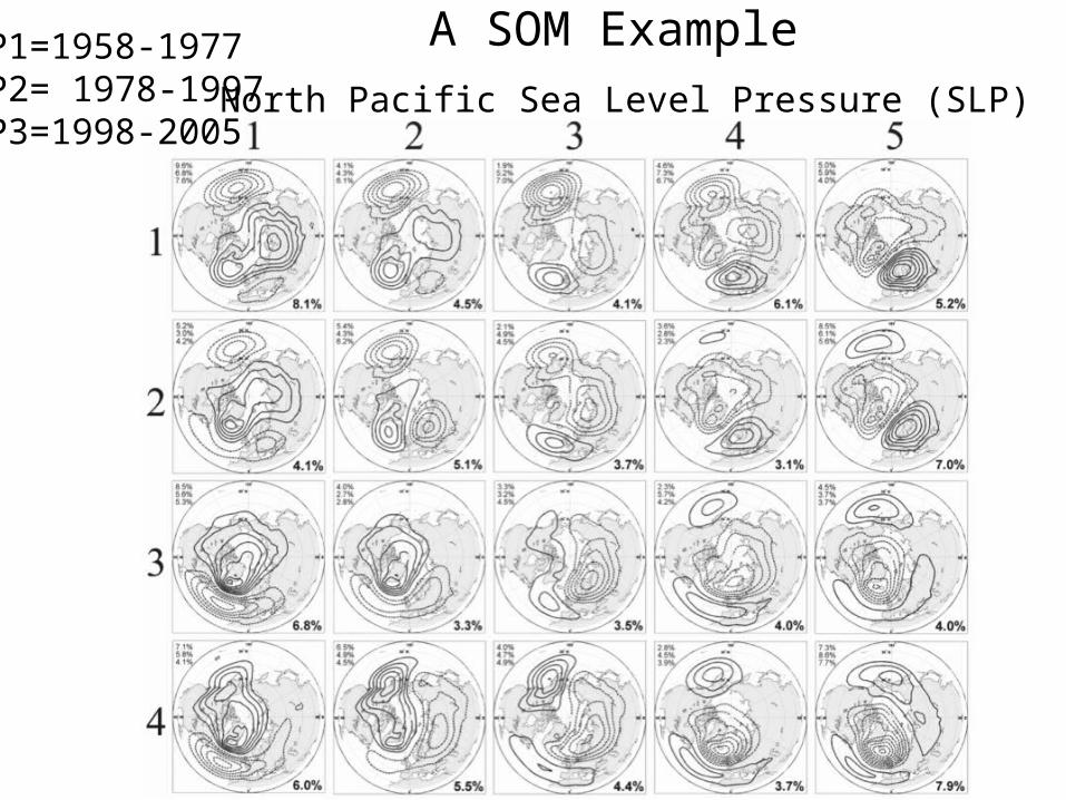
A SOM Example

North Pacific Sea Level Pressure (SLP)

P1=1958-1977P2= 1978-1997P3=1998-2005

Number of SOM patterns

• The number of SOM patterns that we choose is a balance between:

resolution (capturing essential details) & convenience (not too many panels for interpretation)

• Choice on number of SOM also depends upon particular application

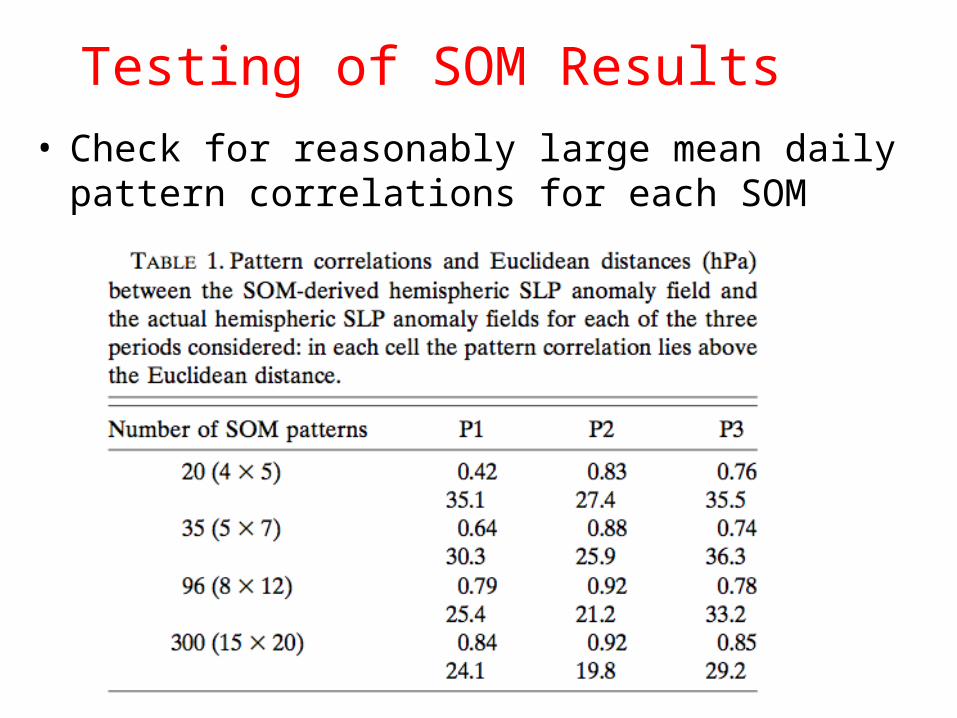
Testing of SOM Results

• Check for reasonably large mean daily pattern correlations for each SOM

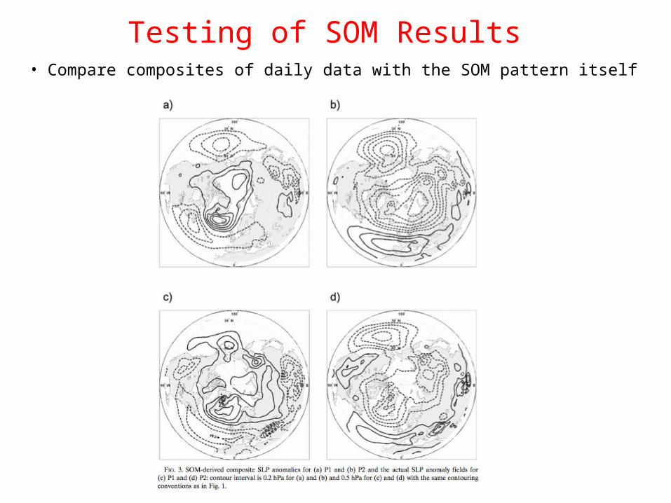
Testing of SOM Results• Compare composites of daily data with the SOM pattern itself

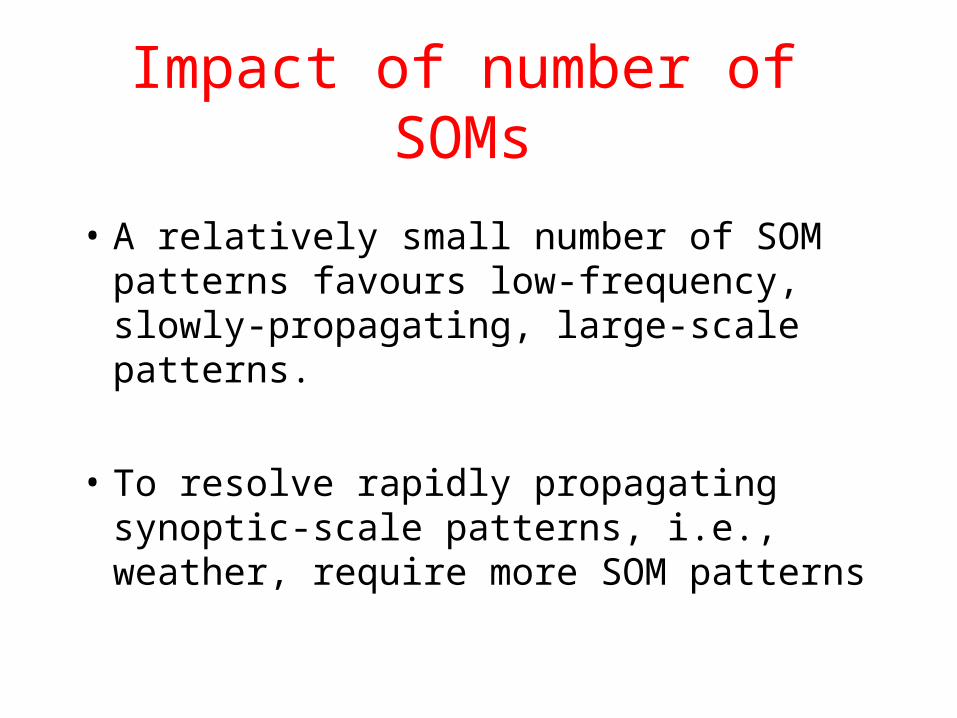
Impact of number of SOMs

• A relatively small number of SOM patterns favours low-frequency, slowly-propagating, large-scale patterns.

• To resolve rapidly propagating synoptic-scale patterns, i.e., weather, require more SOM patterns

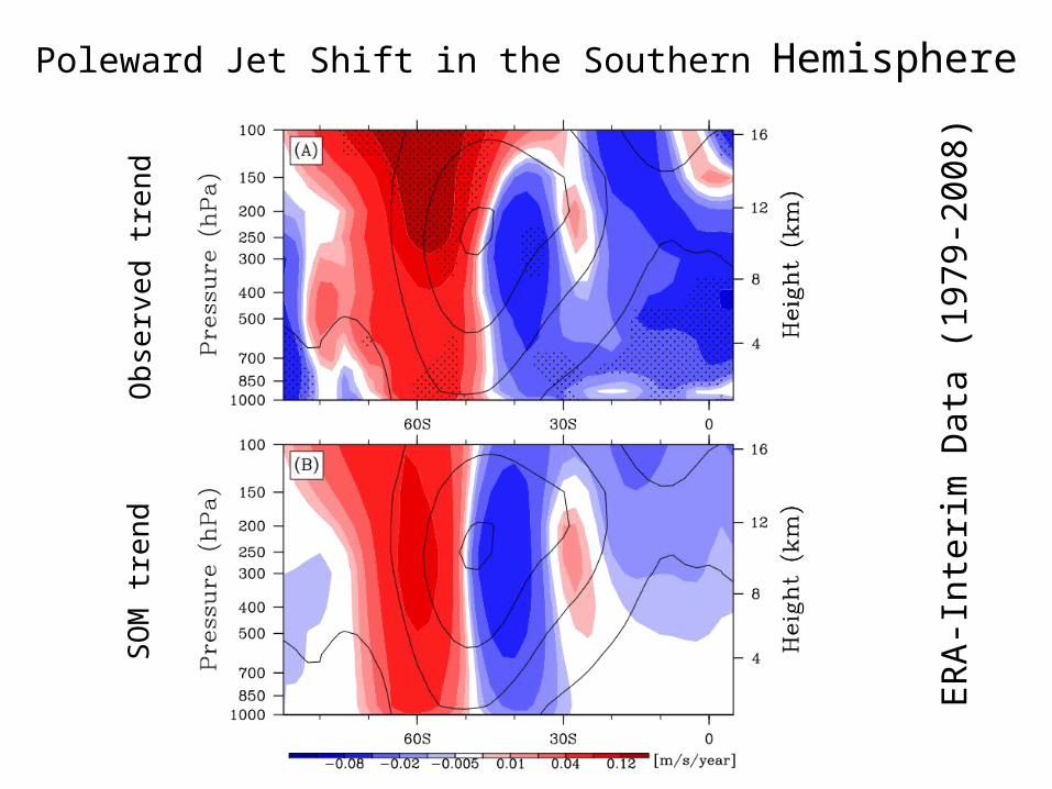
Poleward Jet Shift in the Southern Hemisphere

ER

A-I

nter

im D

ata

(197

9-20

08)

Obs

erve

d tr

end

SO

M tr

end

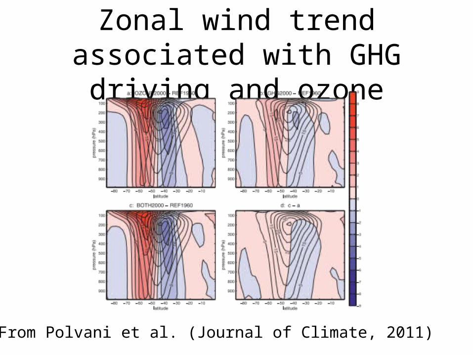
Zonal wind trend associated with GHG driving and ozone

From Polvani et al. (Journal of Climate, 2011)

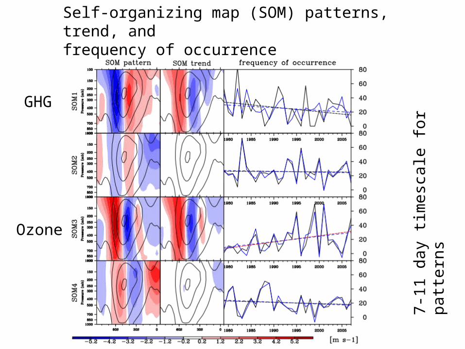
Self-organizing map (SOM) patterns, trend, and frequency of occurrence

7-11

day

tim

esca

le f

or p

atte

rns

GHG

Ozone

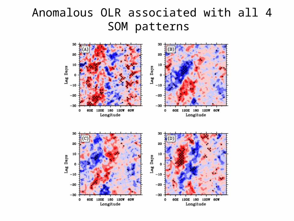
Anomalous OLR associated with all 4 SOM patterns

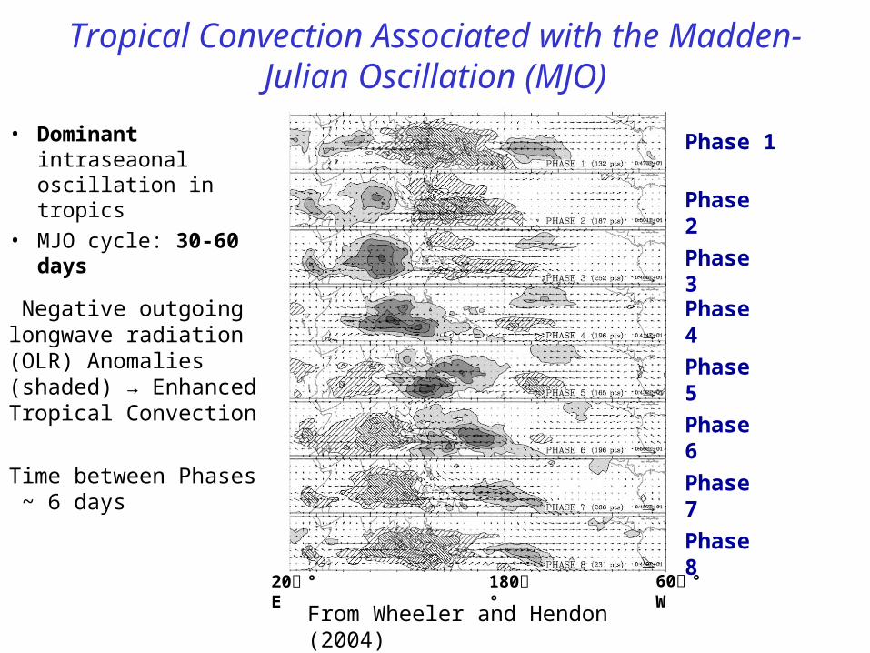
Tropical Convection Associated with the Madden-Julian Oscillation (MJO)

From Wheeler and Hendon (2004)

Negative outgoing longwave radiation (OLR) Anomalies (shaded) → Enhanced Tropical Convection

Phase 1

Phase 2

Phase 3Phase 4

Phase 5

Phase 6

Phase 7

Phase 8

Time between Phases ~ 6 days

180 ۫° 60 ۫°W20 ۫°E

• Dominant intraseaonal oscillation in tropics

• MJO cycle: 30-60 days

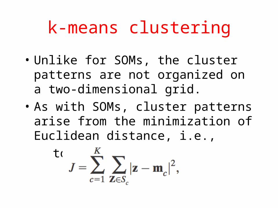
k-means clustering

• Unlike for SOMs, the cluster patterns are not organized on a two-dimensional grid.

• As with SOMs, cluster patterns arise from the minimization of Euclidean distance, i.e.,

to minimize J

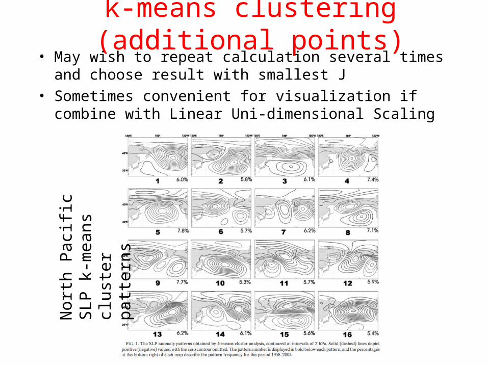
k-means clustering (additional points)• May wish to repeat calculation several times and choose

result with smallest J

• Sometimes convenient for visualization if combine with Linear Uni-dimensional Scaling

Nor

th P

acif

ic S

LP

k-

mea

ns c

lust

er p

atte

rns

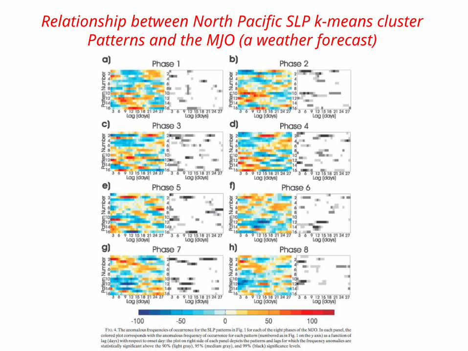
Relationship between North Pacific SLP k-means cluster Patterns and the MJO (a weather forecast)

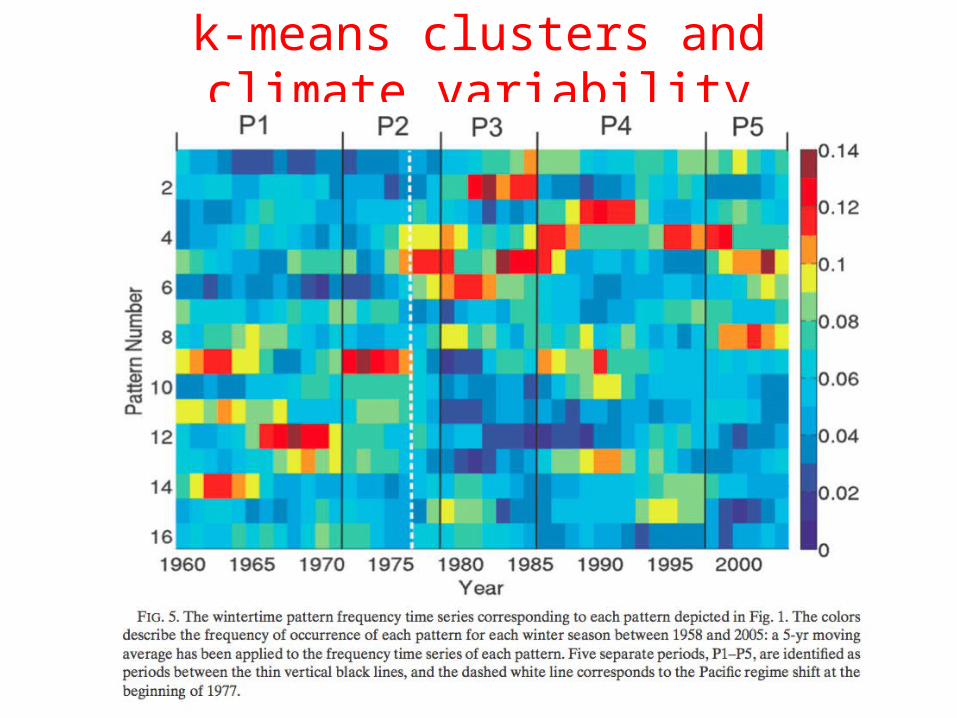
k-means clusters and climate variability

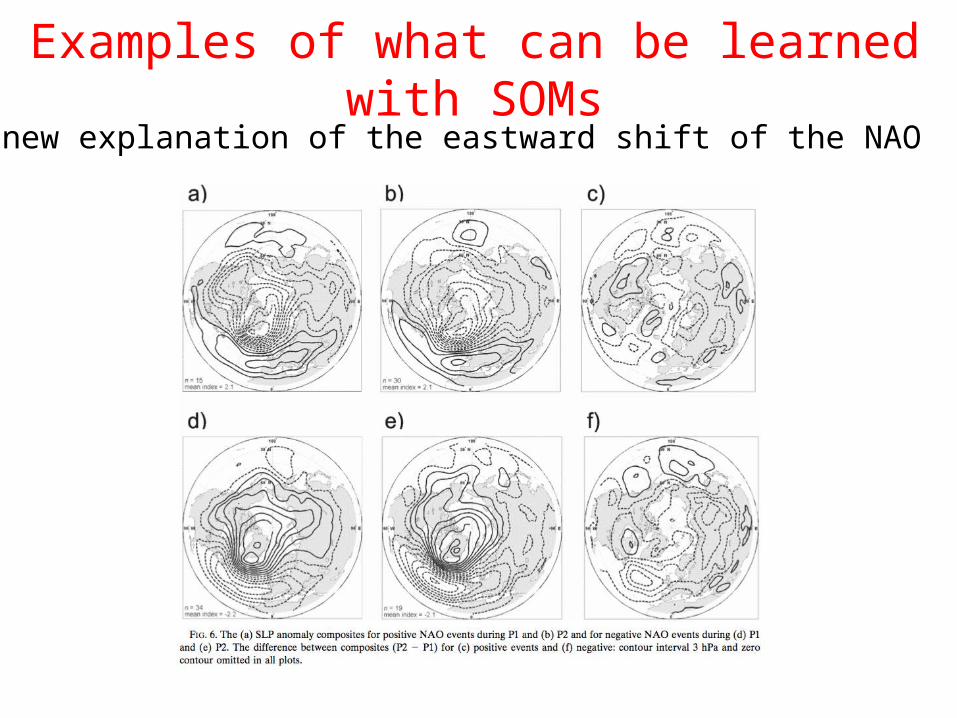
Examples of what can be learned with SOMsA new explanation of the eastward shift of the NAO

Matlab Code

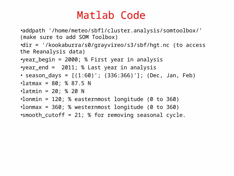
•addpath '/home/meteo/sbf1/cluster.analysis/somtoolbox/’ (make sure to add SOM Toolbox)•dir = '/kookaburra/s0/grayvireo/s3/sbf/hgt.nc (to access the Reanalysis data)•year_begin = 2000; % First year in analysis•year_end = 2011; % Last year in analysis• season_days = [(1:60)'; (336:366)']; (Dec, Jan, Feb)•latmax = 80; % 87.5 N•latmin = 20; % 20 N•lonmin = 120; % easternmost longitude (0 to 360)•lonmax = 360; % westernmost longitude (0 to 360)•smooth_cutoff = 21; % for removing seasonal cycle.

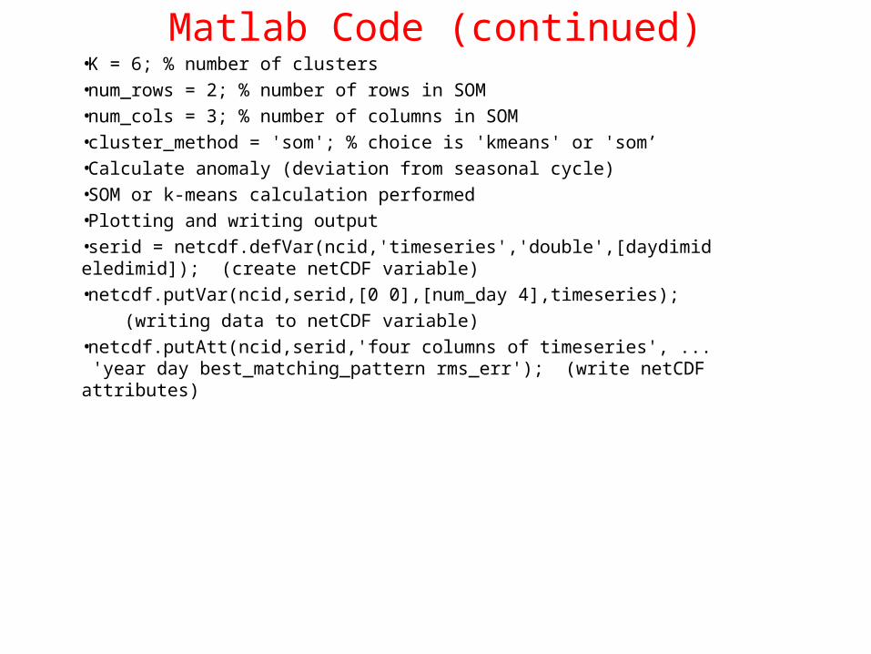
Matlab Code (continued) •K = 6; % number of clusters•num_rows = 2; % number of rows in SOM•num_cols = 3; % number of columns in SOM•cluster_method = 'som'; % choice is 'kmeans' or 'som’•Calculate anomaly (deviation from seasonal cycle)•SOM or k-means calculation performed•Plotting and writing output•serid = netcdf.defVar(ncid,'timeseries','double',[daydimid eledimid]); (create netCDF variable)•netcdf.putVar(ncid,serid,[0 0],[num_day 4],timeseries);

(writing data to netCDF variable)•netcdf.putAtt(ncid,serid,'four columns of timeseries', ... 'year day best_matching_pattern rms_err'); (write netCDF attributes)

2X3 SOM map (500-hPa height)

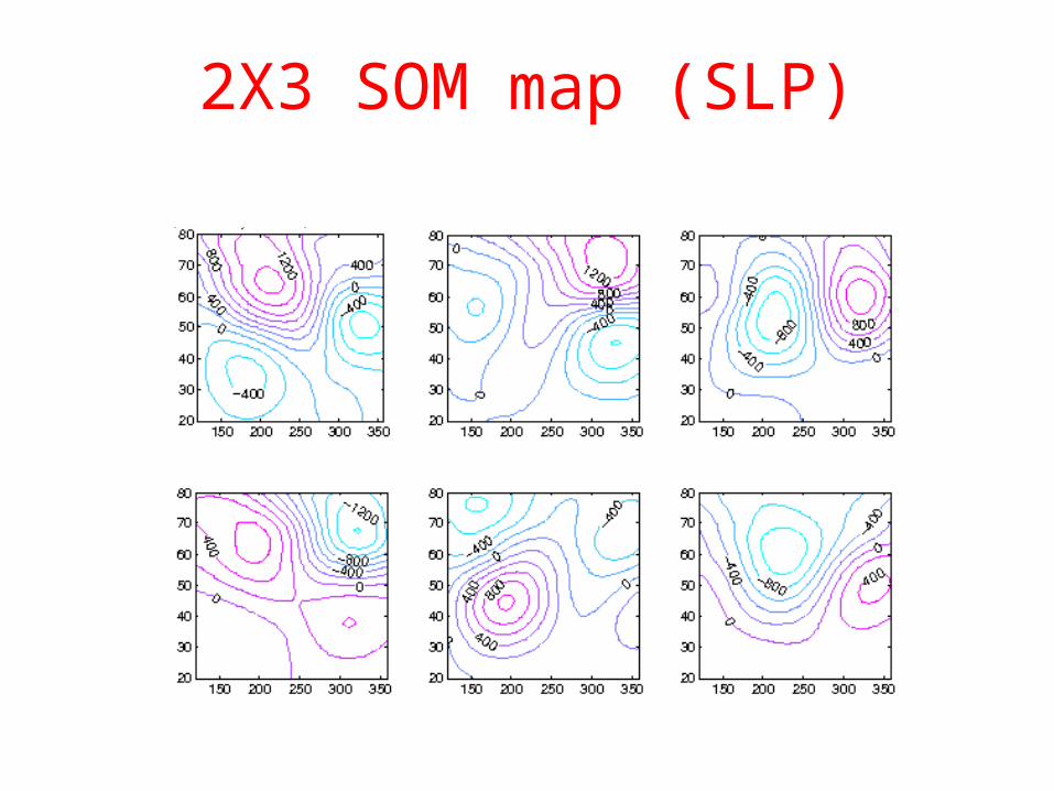
2X3 SOM map (SLP)