Self-Organizing Maps (SOMs): Proposed RMIP Diagnosis
140
Self-Organizing Maps Self-Organizing Maps (SOMs): (SOMs): Proposed RMIP Diagnosis Proposed RMIP Diagnosis W. J. Gutowski, Jr. W. J. Gutowski, Jr. Iowa State University Iowa State University RMIP (December 2001) thanks to: thanks to: ei ei , , F. Otieno F. Otieno , Z. Pan, R. W. Arritt, E. S. T , Z. Pan, R. W. Arritt, E. S. T
-
Upload
austin-york -
Category
Documents
-
view
24 -
download
0
description
Self-Organizing Maps (SOMs): Proposed RMIP Diagnosis. W. J. Gutowski, Jr. Iowa State University. with thanks to: H. Wei , F. Otieno , Z. Pan, R. W. Arritt, E. S. Takle. RMIP(December 2001). Outline. Background Example 1: Precipitation simulation versus observations - PowerPoint PPT Presentation
Transcript of Self-Organizing Maps (SOMs): Proposed RMIP Diagnosis

Self-Organizing Maps (SOMs):Self-Organizing Maps (SOMs):Proposed RMIP DiagnosisProposed RMIP Diagnosis
W. J. Gutowski, Jr.W. J. Gutowski, Jr.Iowa State UniversityIowa State University
RMIP (December 2001)
with thanks to: with thanks to: H. WeiH. Wei, , F. OtienoF. Otieno, Z. Pan, R. W. Arritt, E. S. Takle, Z. Pan, R. W. Arritt, E. S. Takle
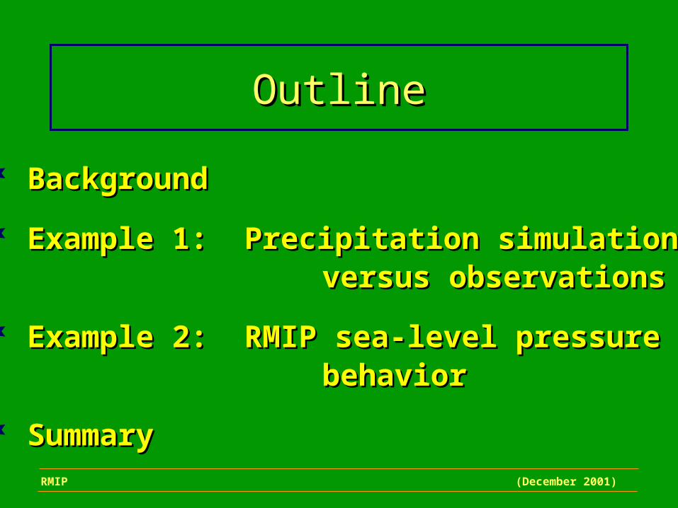
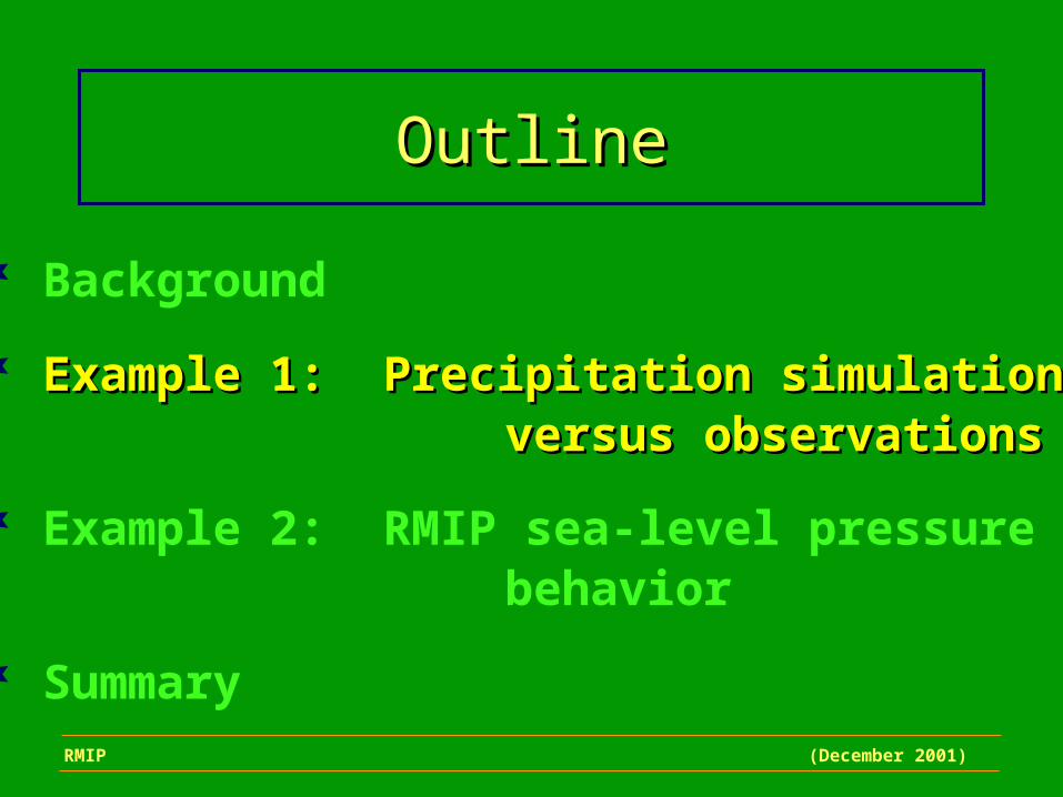
OutlineOutline
BackgroundBackground
Example 1: Precipitation simulation Example 1: Precipitation simulation versus observationsversus observations
Example 2: RMIP sea-level pressure Example 2: RMIP sea-level pressure behaviorbehavior
SummarySummaryRMIP (December 2001)

Self-Organizing Maps:Background
Set of maps
• Show characteristic data structures
• Trained to distribution of data
• Give 2-D projection of higher order map space
• Are approximately continuous
• Basis in Artificial Neural Nets
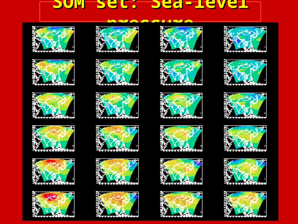
SOM set: Sea-level pressureSOM set: Sea-level pressure
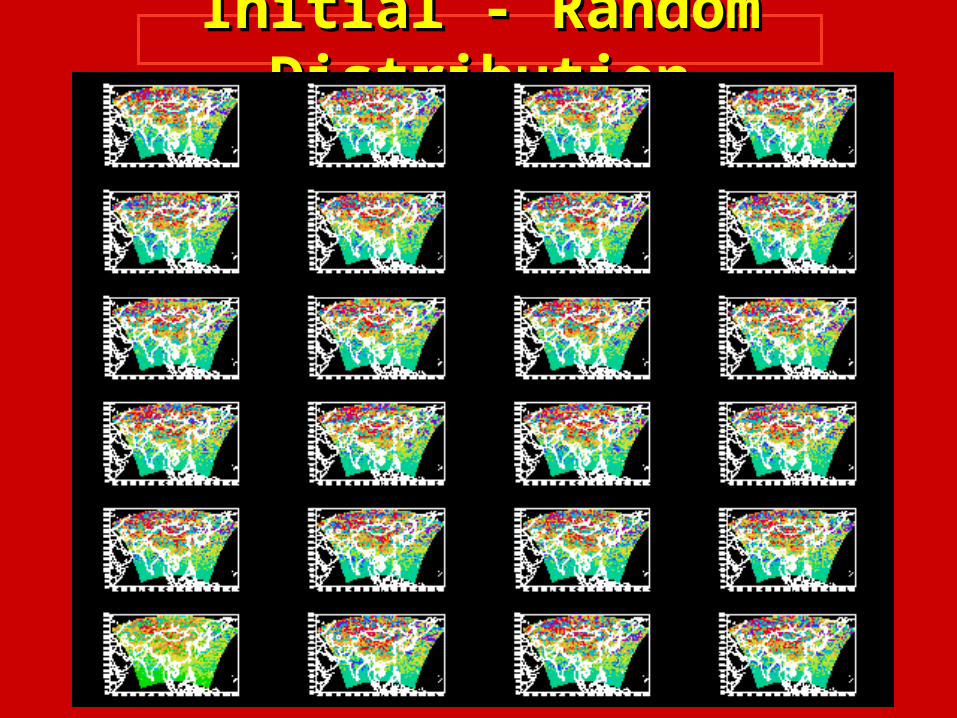
Initial - Random DistributionInitial - Random Distribution

Apply input sequence of maps: Apply input sequence of maps: exampleexample

Compare sample Compare sample to ...to ...
… … existing setexisting set

Find closest map ...Find closest map ...(here - smallest RMS (here - smallest RMS
difference)difference)
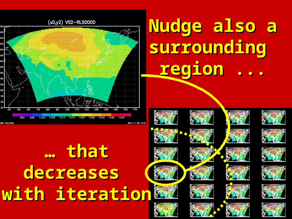
… … and it nudge and it nudge toward sampletoward sample

Nudge also a Nudge also a surrounding surrounding
region ...region ...
… … that decreases that decreases with iterationwith iteration
… … that decreases that decreases with iterationwith iteration
Nudge also a Nudge also a surrounding surrounding
region ...region ...

… … that decreases that decreases with iterationwith iteration
Nudge also a Nudge also a surrounding surrounding
region ...region ...
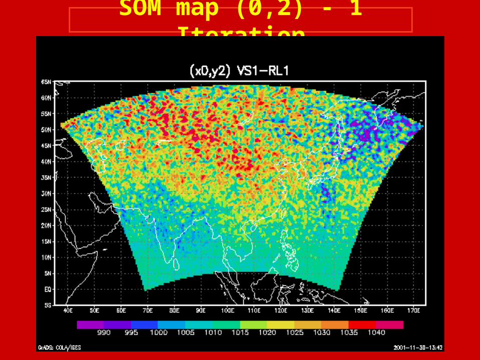
SOM map (0,2) - 1 Iteration
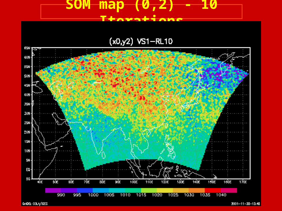
SOM map (0,2) - 10 Iterations
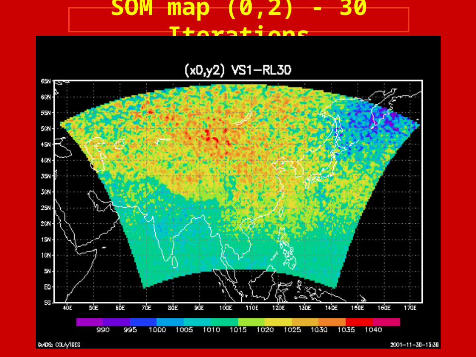
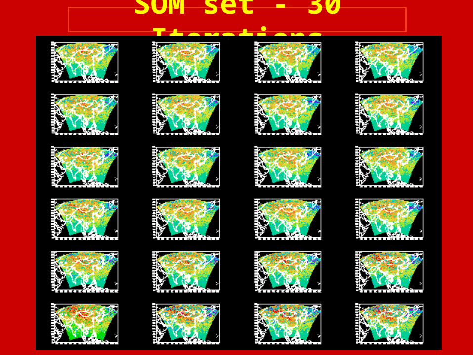
SOM map (0,2) - 30 Iterations
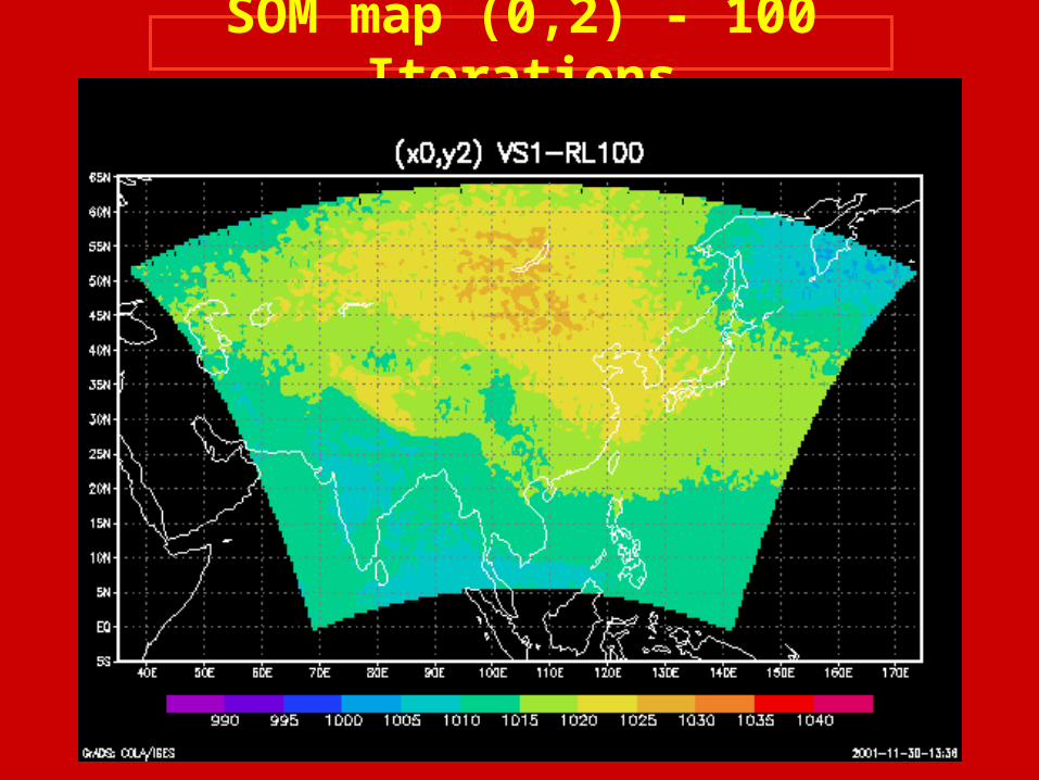
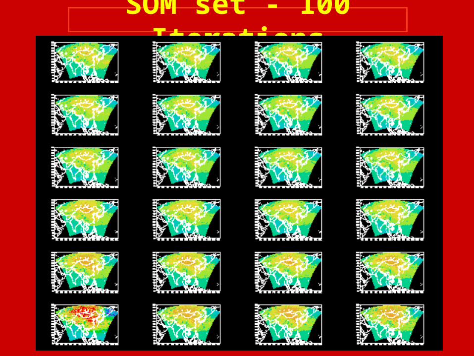
SOM map (0,2) - 100 Iterations
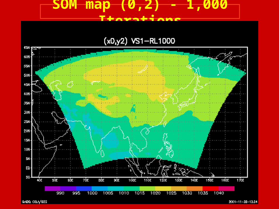
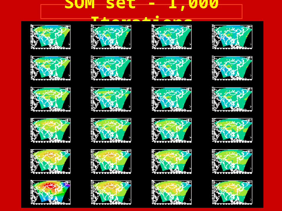
SOM map (0,2) - 1,000 Iterations
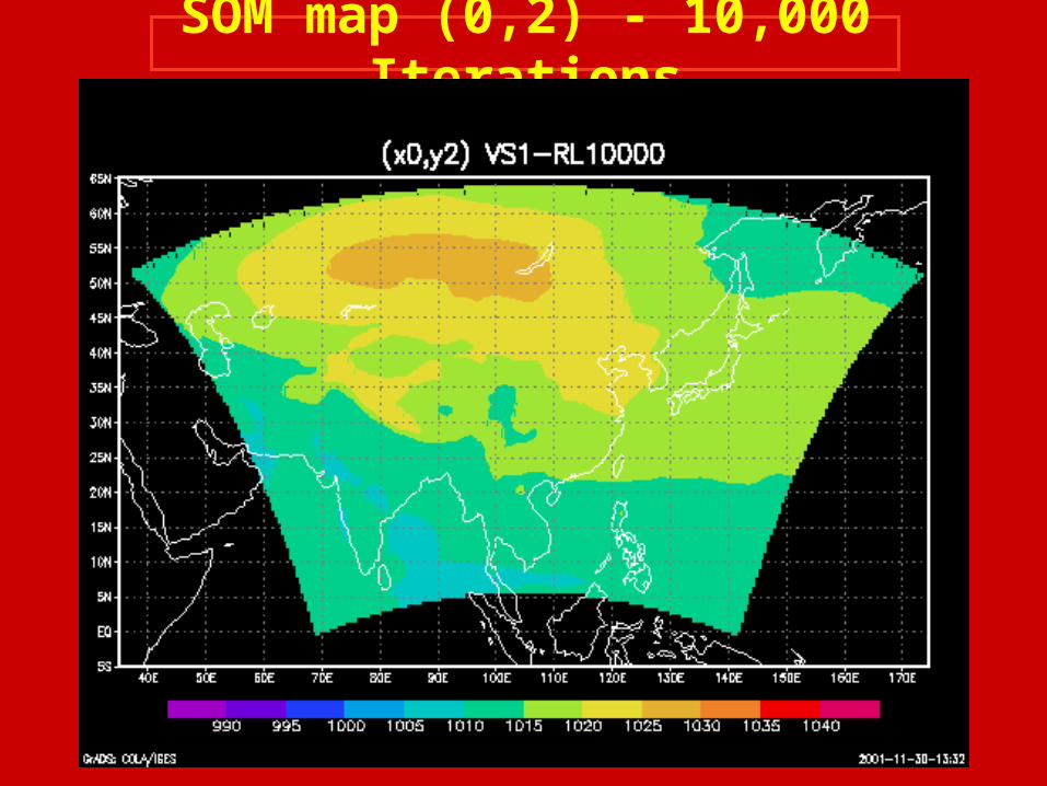
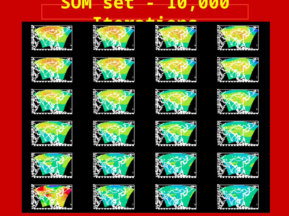
SOM map (0,2) - 10,000 Iterations
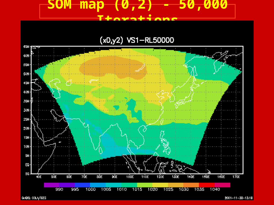
SOM map (0,2) - 50,000 Iterations

SOM map (0,2) - 100,000 Iterations
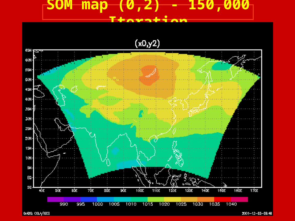
SOM map (0,2) - 150,000 Iteration
OutlineOutline
Background
Example 1: Precipitation simulation Example 1: Precipitation simulation versus observationsversus observations
Example 2: RMIP sea-level pressure behavior
SummaryRMIP (December 2001)
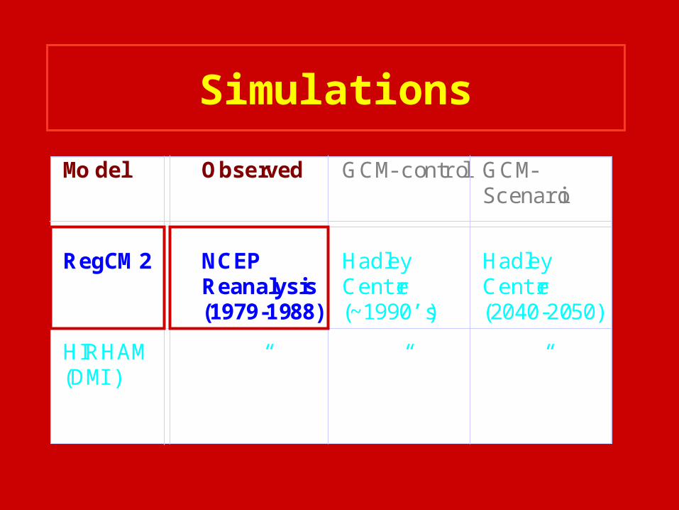
Simulations
Model Observed GCM-control GCM-Scenario
RegCM2 NCEPReanalysis(1979-1988)
HadleyCentre(~1990’s)
HadleyCentre(2040-2050)
HIRHAM(DMI)
“ “ “
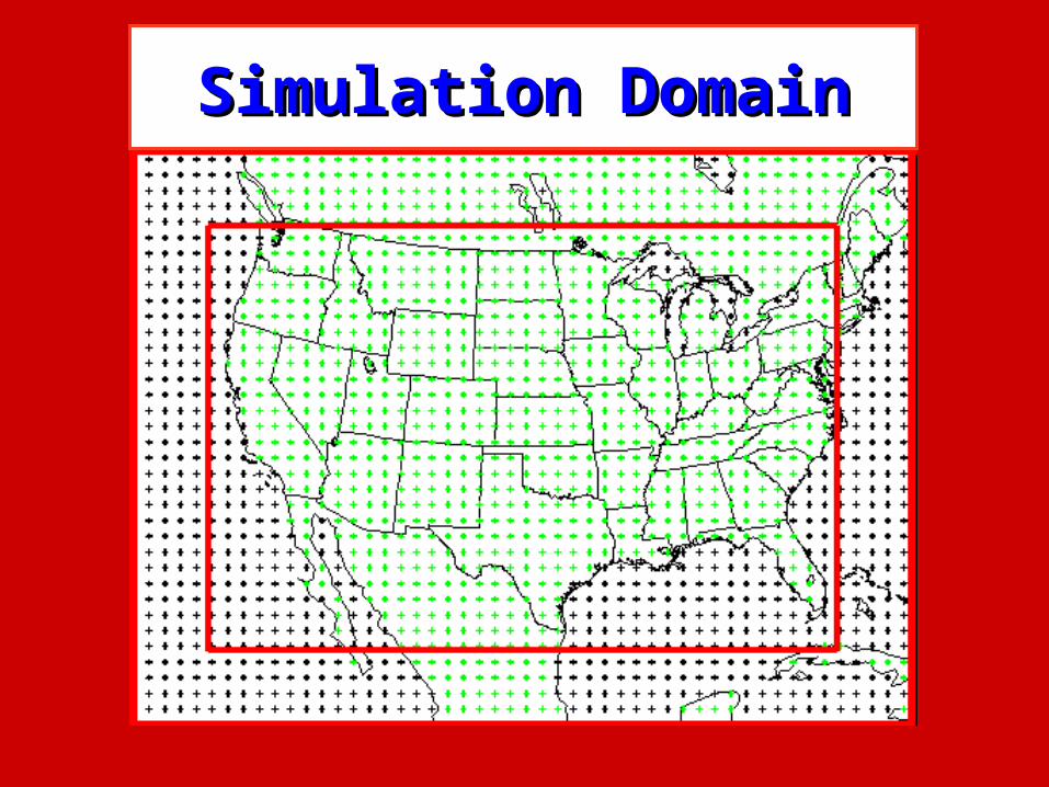
Simulation DomainSimulation Domain

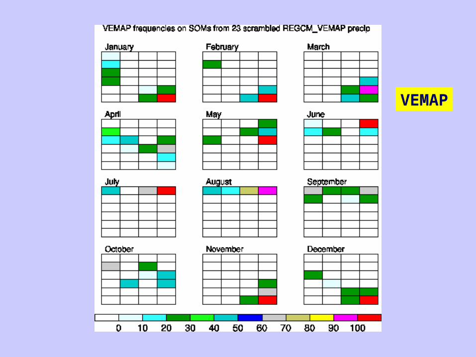
SOM: RegCM2 & VEMAP Precipitation

1
2
SOM: RegCM2 & VEMAP Precipitation

1
2
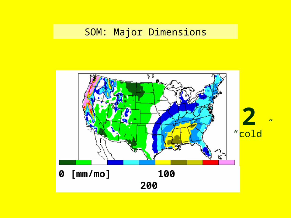
SOM: Major Dimensions
0 [mm/mo] 100 200
“warm”
“cold”

RegCM2
VEMAP
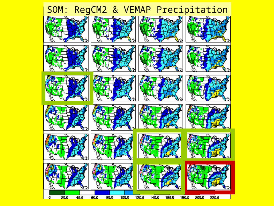
SOM: RegCM2 & VEMAP Precipitation

SOM: RegCM2 & VEMAP Precipitation

SOM Trajectories
RegCM
VEMAP
J-J-A

SOM Trajectories
RegCM
D-J-F
VEMAP
D-J-F
RegCM
VEMAP
J-J-A
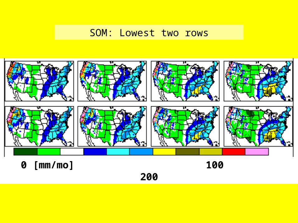
SOM: Lowest two rows
0 [mm/mo] 100 200

Trajectory Separation by Month

OutlineOutline
Background
Example 1: Precipitation simulation versus observations
Example 2: RMIP sea-level pressure Example 2: RMIP sea-level pressure behaviorbehavior
SummaryRMIP (December 2001)

RMIP Sea-level Pressure
Input:
ISU MM5 simulation
Sampled daily at 12 UTC
18 months 549 samples
Unadjusted (e.g., no filtering,
scaling, etc.)
0
500
1000
1500
2000
100
101
102
103
104
105
Mean Sq. Error [hPa*hPa]
Iterations
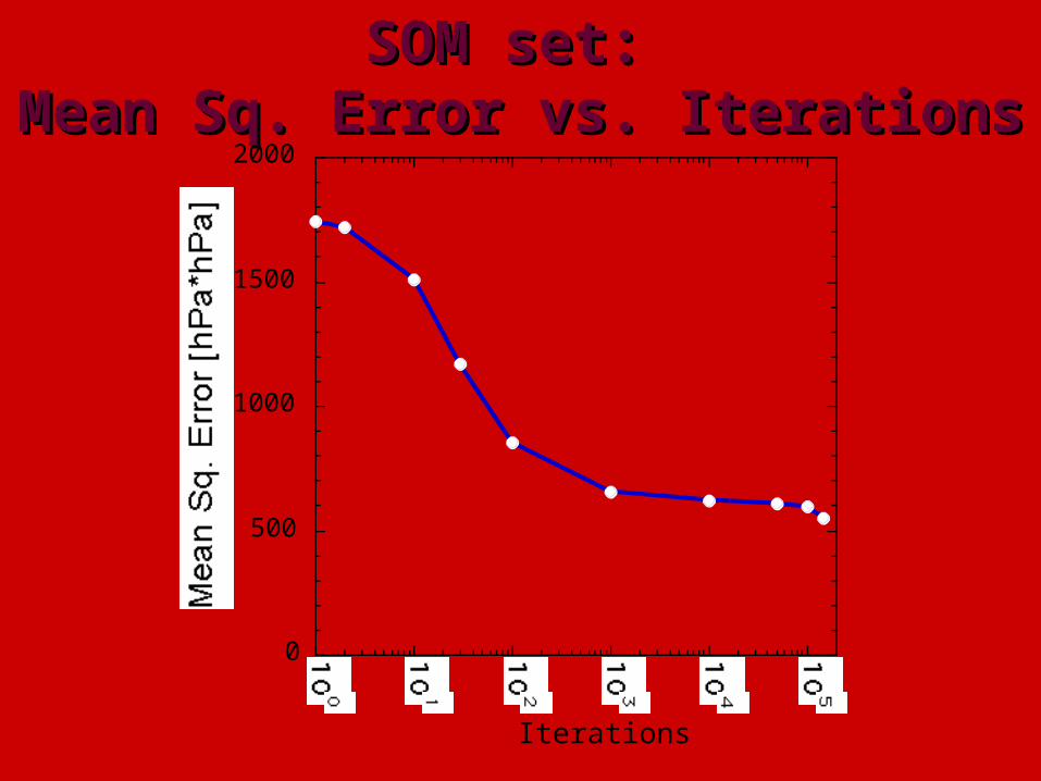
SOM set: SOM set: Mean Sq. Error vs. IterationsMean Sq. Error vs. Iterations

SOM set: Sea-level pressureSOM set: Sea-level pressure

“Nearest map” Frequency
Even distribution
0.04
5
4
3
2
1
00 1 2 3

Mean Squared Error of Fit - All Days
5
4
3
2
1
0[hPa2]
0 1 2 3
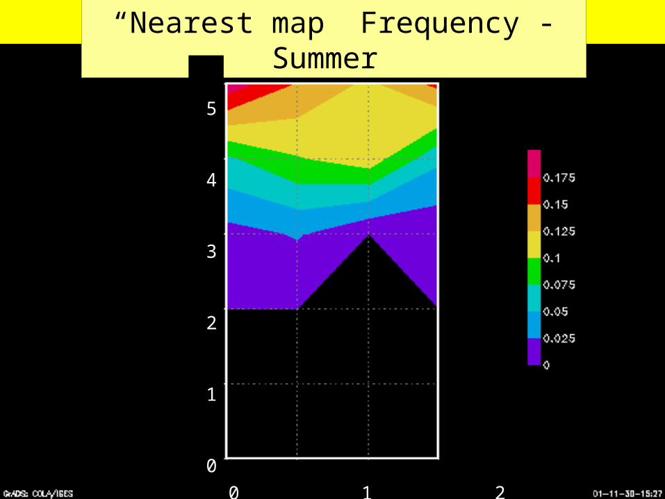
“Nearest map” Frequency - Summer
5
4
3
2
1
0
0 1 2 3

“Nearest map” Frequency - Fall
5
4
3
2
1
0
0 1 2 3
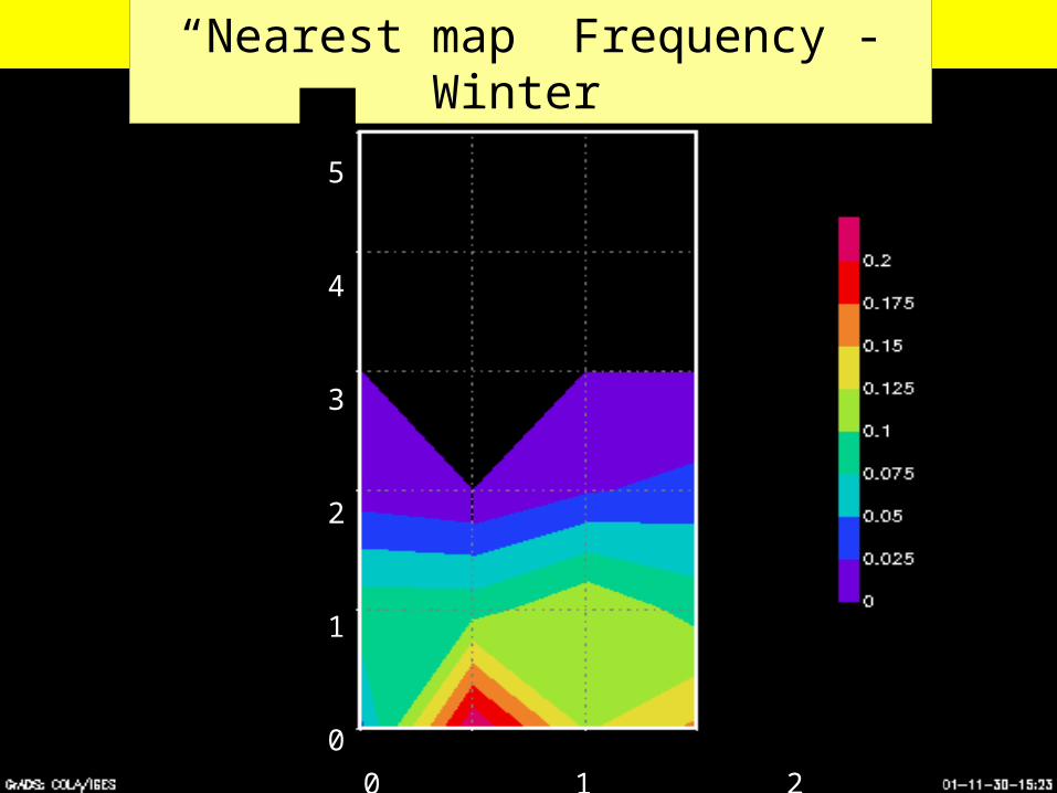
“Nearest map” Frequency - Winter
5
4
3
2
1
0
0 1 2 3
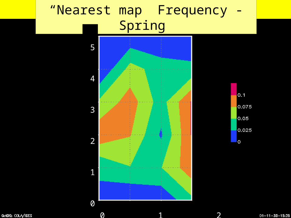
“Nearest map” Frequency - Spring
5
4
3
2
1
0
0 1 2 3

Summer High Frequency Map

Fall High Frequency Map

Winter High Frequency Map
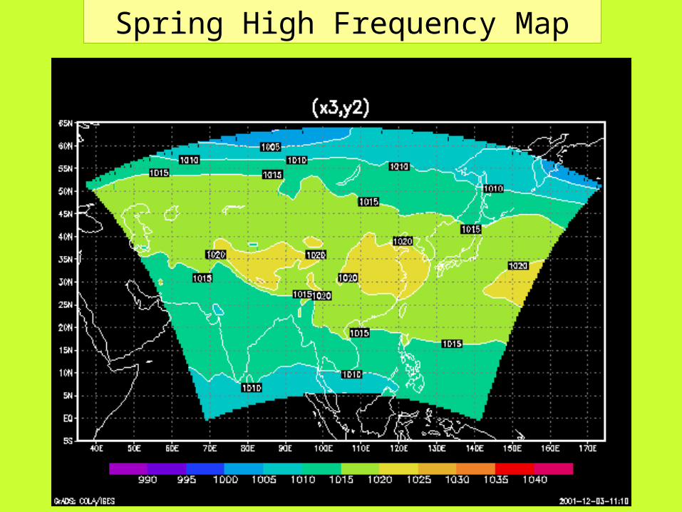
Spring High Frequency Map
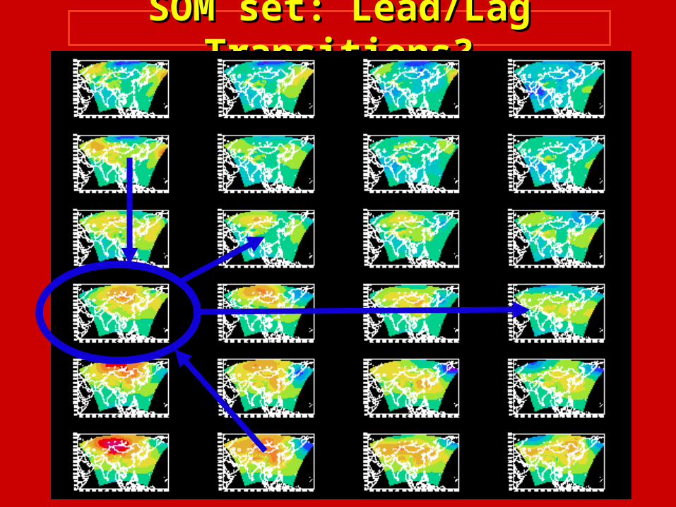
SOM set: Lead/Lag Transitions?SOM set: Lead/Lag Transitions?

Frequency of Maps that Lead: 90 DaysFrequency of Maps that Lead: 90 Days
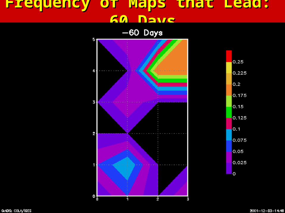
Frequency of Maps that Lead: 60 DaysFrequency of Maps that Lead: 60 Days

Frequency of Maps that Lead: 30 DaysFrequency of Maps that Lead: 30 Days
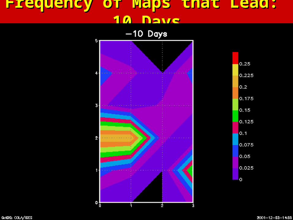
Frequency of Maps that Lead: 10 DaysFrequency of Maps that Lead: 10 Days
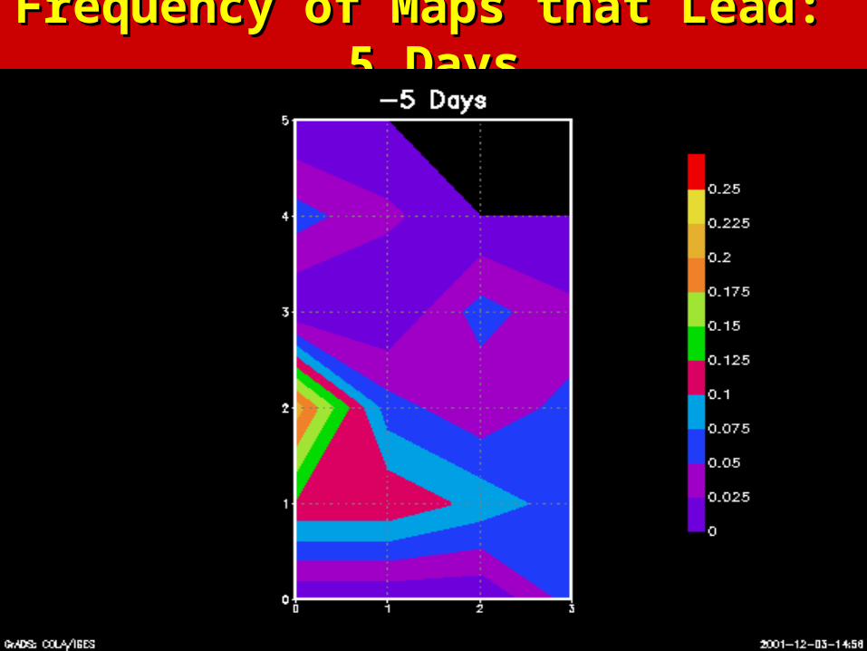
Frequency of Maps that Lead: 5 DaysFrequency of Maps that Lead: 5 Days

Frequency of Maps that Lead: 4 DaysFrequency of Maps that Lead: 4 Days

Frequency of Maps that Lead: 3 DaysFrequency of Maps that Lead: 3 Days
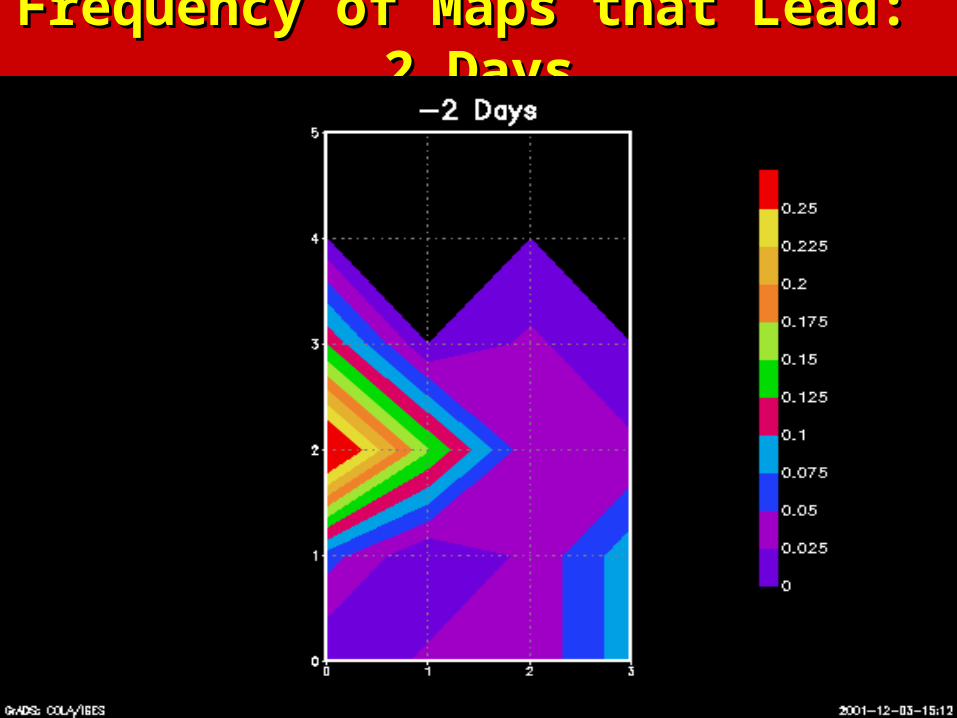
Frequency of Maps that Lead: 2 DaysFrequency of Maps that Lead: 2 Days
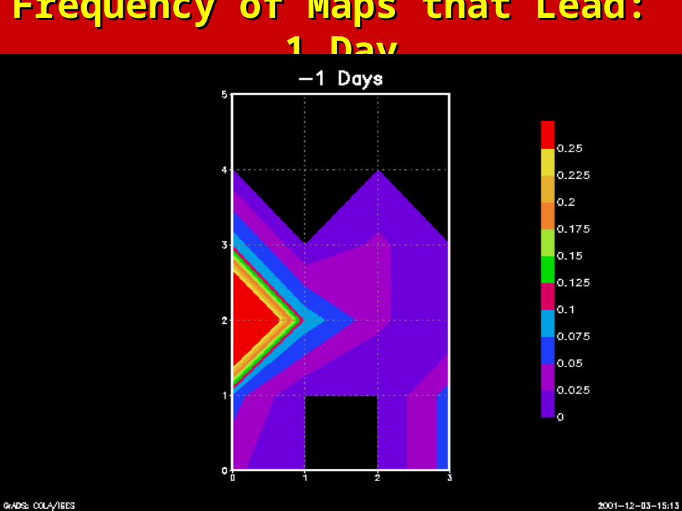
Frequency of Maps that Lead: 1 DayFrequency of Maps that Lead: 1 Day

Frequency of Maps that Lag: 1 DayFrequency of Maps that Lag: 1 Day
55%55%
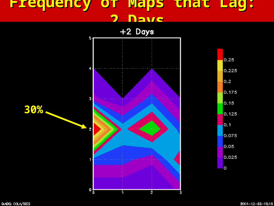
Frequency of Maps that Lag: 2 DaysFrequency of Maps that Lag: 2 Days
30%30%

Frequency of Maps that Lag: 3 DaysFrequency of Maps that Lag: 3 Days
21%21%

Frequency of Maps that Lag: 4 DaysFrequency of Maps that Lag: 4 Days
18%18%

Frequency of Maps that Lag: 5 DaysFrequency of Maps that Lag: 5 Days
21%21%

Frequency of Maps that Lag: 10 DaysFrequency of Maps that Lag: 10 Days
21%21%

Frequency of Maps that Lag: 30 DaysFrequency of Maps that Lag: 30 Days
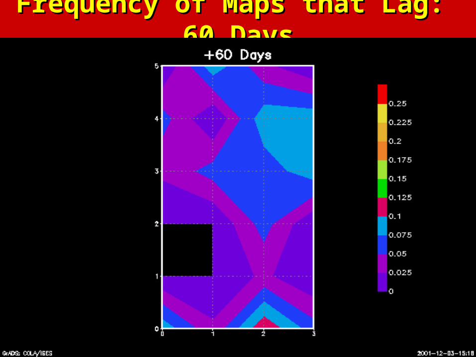
Frequency of Maps that Lag: 60 DaysFrequency of Maps that Lag: 60 Days

Frequency of Maps that Lag: 90 DaysFrequency of Maps that Lag: 90 Days

Alternatives
Band-, low-, high-pass filter
Multiple data types
Input “maps” in (x,t), (y,t), (x,t), etc.
...
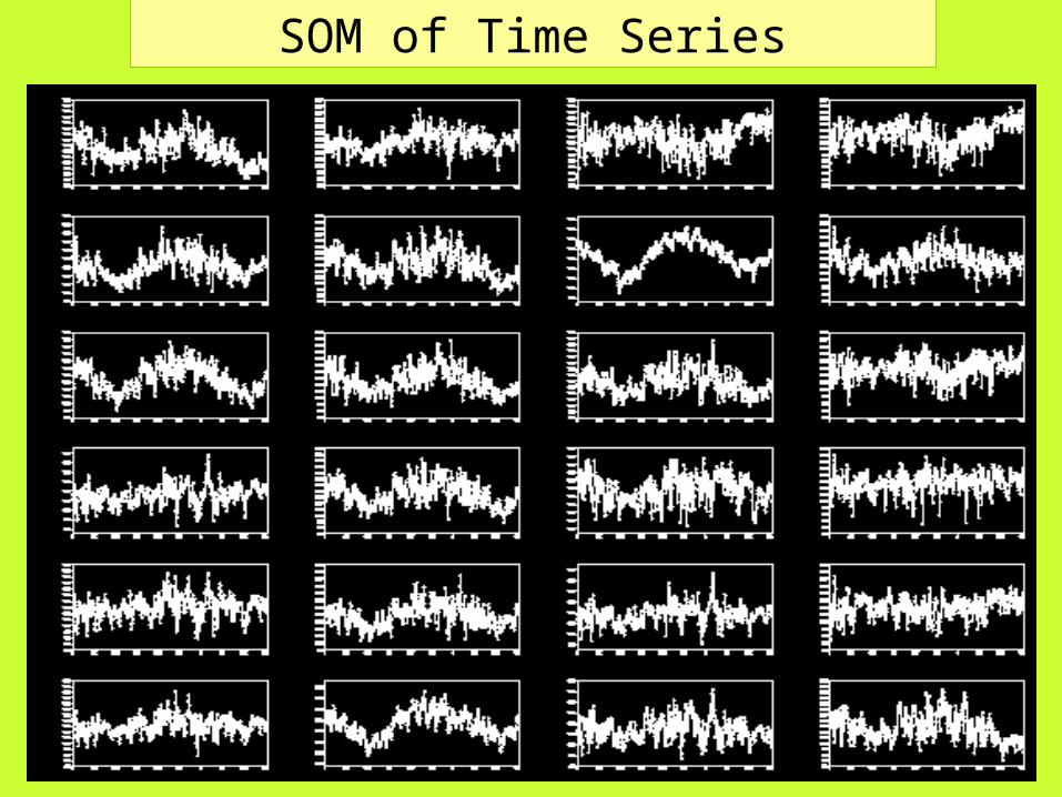
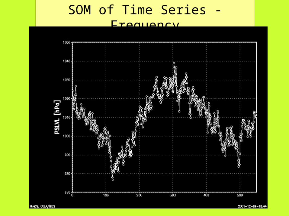
SOM of Time Series
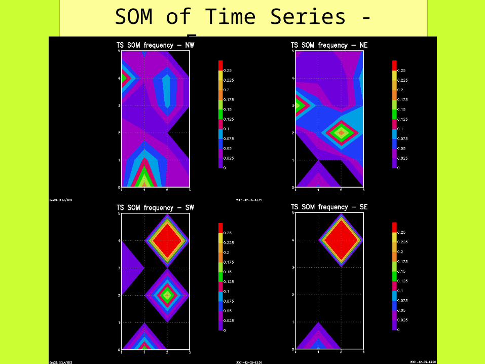
SOM of Time Series - Frequency
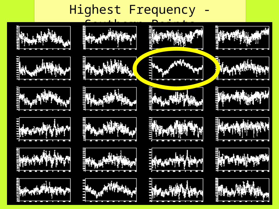
Highest Frequency - Southern Points
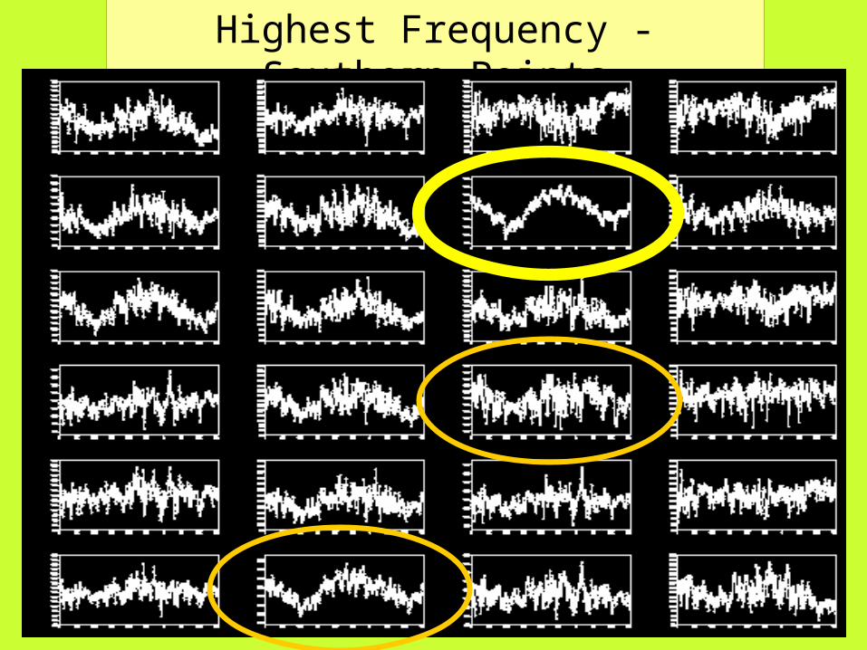
Highest Frequency - Southern Points
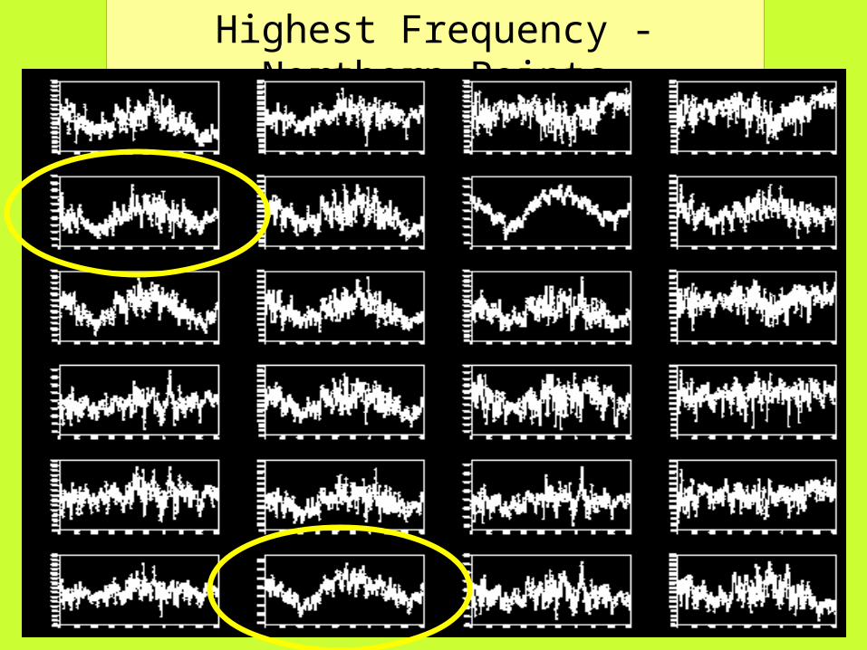
Highest Frequency - Northern Points

Highest Frequency - Northern Points
OutlineOutline
Background
Example 1: Precipitation simulation versus observations
Example 2: RMIP sea-level pressure behavior
SummarySummaryRMIP (December 2001)

Summary
(1) Self-Organizing Maps provide characteristic
spatial distributions
evolution in time
frequency of occurrence
RMIP (December 2001)

Summary
(1) Self-Organizing Maps provide characteristic
spatial distributions
evolution in time
frequency of occurrence
(2) Caution: SOMs are a tool, not an answer.
The user must supply interpretation and care in use.
RMIP (December 2001)
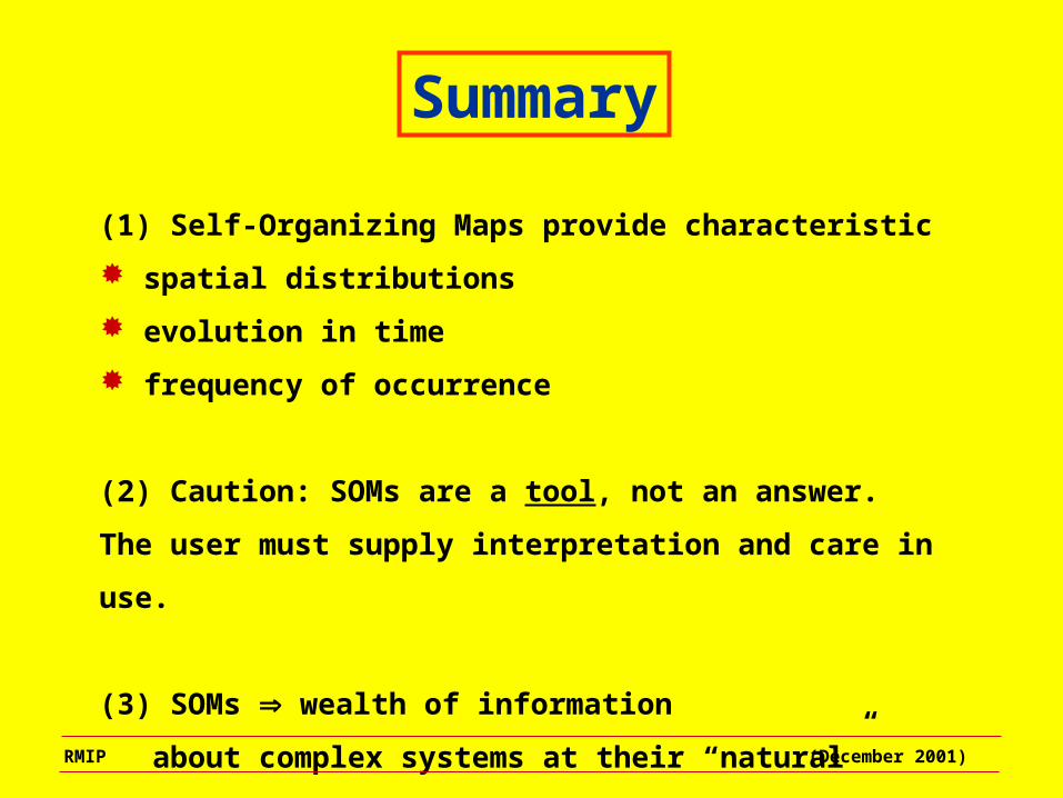
Summary
(1) Self-Organizing Maps provide characteristic
spatial distributions
evolution in time
frequency of occurrence
(2) Caution: SOMs are a tool, not an answer.
The user must supply interpretation and care in use.
(3) SOMs wealth of information
about complex systems at their “natural” scale.
RMIP (December 2001)

AcknowledgmentsAcknowledgments
Electric Power Research Institute Electric Power Research Institute (EPRI)(EPRI)
U.S. National Oceanic and Atmospheric U.S. National Oceanic and Atmospheric Administration (NOAA)Administration (NOAA)
RMIP (December 2001)

EXTRA
SLIDES
2
SOM: Major Dimensions
0 [mm/mo] 100 200
“cold”

SOM set - 1 Iteration

SOM set - 10 Iterations
SOM set - 30 Iterations
SOM set - 100 Iterations
SOM set - 1,000 Iterations
SOM set - 10,000 Iterations

SOM set - 50,000 Iterations

SOM set - 100,000 Iterations
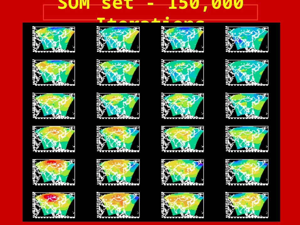
SOM set - 150,000 Iterations

“Nearest map” Frequency - Summer/1
5
4
3
2
1
0
0 1 2 3
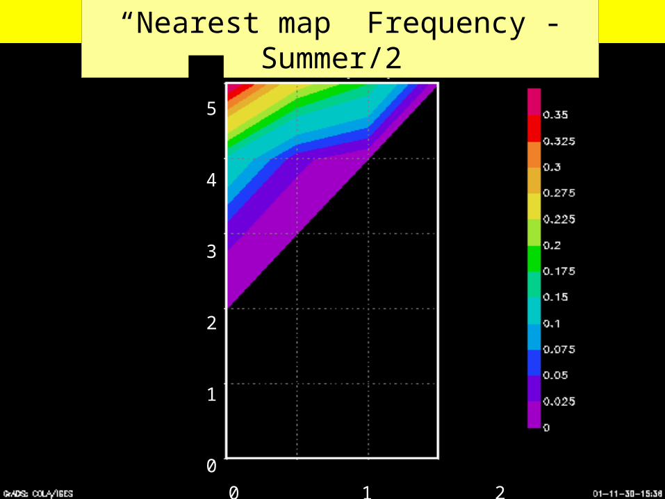
“Nearest map” Frequency - Summer/2
5
4
3
2
1
0
0 1 2 3
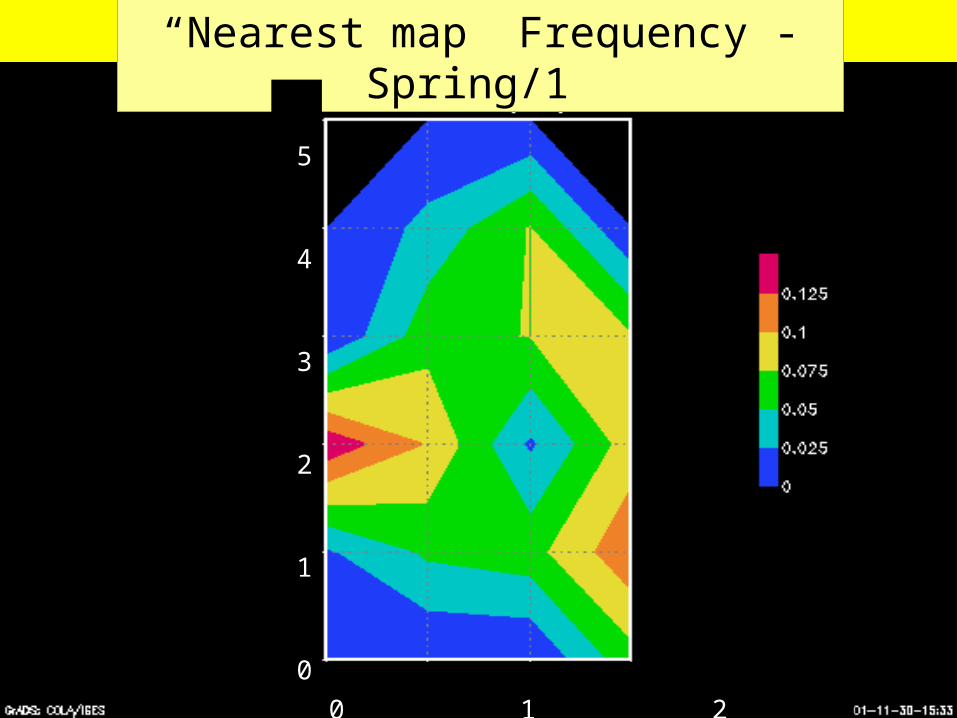
“Nearest map” Frequency - Spring/1
5
4
3
2
1
0
0 1 2 3
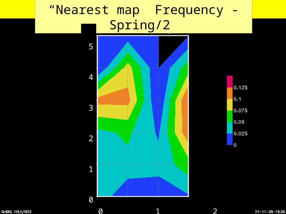
“Nearest map” Frequency - Spring/2
5
4
3
2
1
0
0 1 2 3

SOM of Time Series - Frequency
SOM of Time Series - Frequency

Simulations
Model Observed GCM-control GCM-Scenario
RegCM2 NCEPReanalysis(1979-1988)
HadleyCentre(~1990’s)
HadleyCentre(2040-2050)
HIRHAM(DMI)
“ “ “
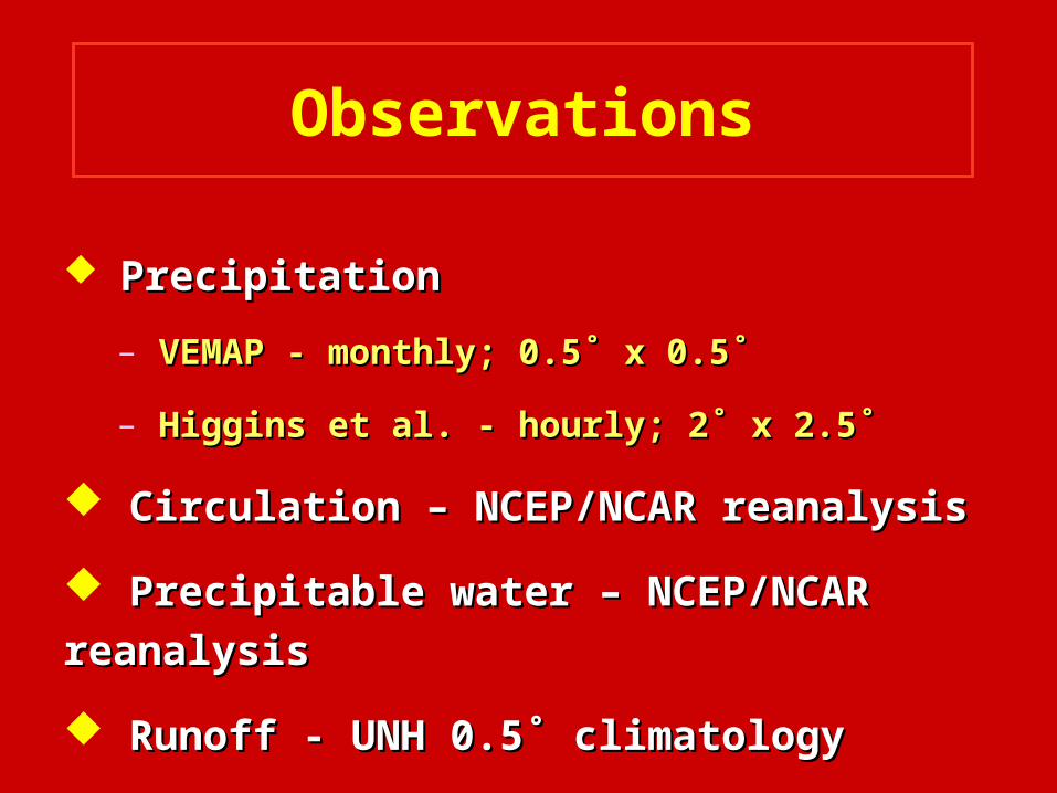
PrecipitationPrecipitation
– VEMAP - monthly; 0.5˚ x 0.5˚VEMAP - monthly; 0.5˚ x 0.5˚
– Higgins et al. - hourly; 2˚ x 2.5˚Higgins et al. - hourly; 2˚ x 2.5˚
Circulation – NCEP/NCAR reanalysisCirculation – NCEP/NCAR reanalysis
Precipitable water – NCEP/NCAR reanalysisPrecipitable water – NCEP/NCAR reanalysis
Runoff - UNH 0.5˚ climatologyRunoff - UNH 0.5˚ climatology
Observations
SASAS (September 2001)
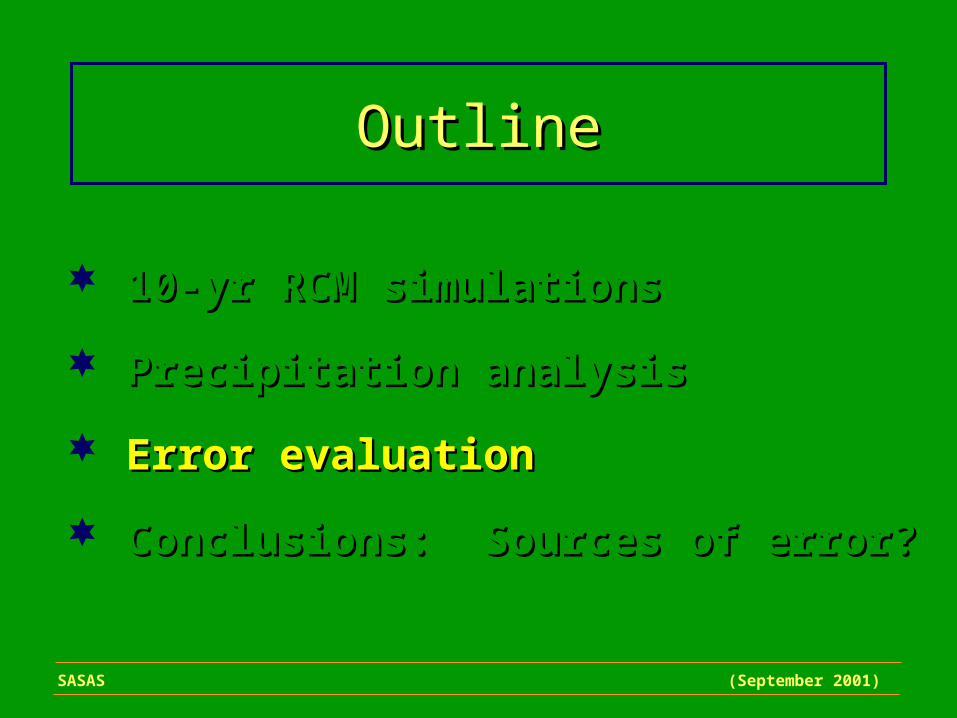
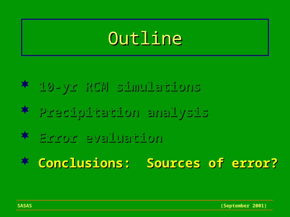
OutlineOutline
10-yr RCM simulations10-yr RCM simulations
Precipitation analysisPrecipitation analysis
Error evaluationError evaluation
Conclusions: Sources of error?Conclusions: Sources of error?

Bias: average differenceBias: average difference
Bias Score: intensity “spectrum”Bias Score: intensity “spectrum”
SOM: SOM: pattern differencepattern difference
Diagnoses

Precip.Bias by Month & Location
-2 0 2 4 [mm/d]

-40
0
1979 1981 1983 1985 1987Year
WINTER SPRING
SUMMER FALL
Season’s Bias by Year~ south-central US ~
(“Fall” = Sep-Oct-Nov, etc.)

(“Score” ~ relative exceeding of threshold)
Bias Score by LocationThreshold = 1 mm/d
(“Score” ~ relative exceeding of threshold)
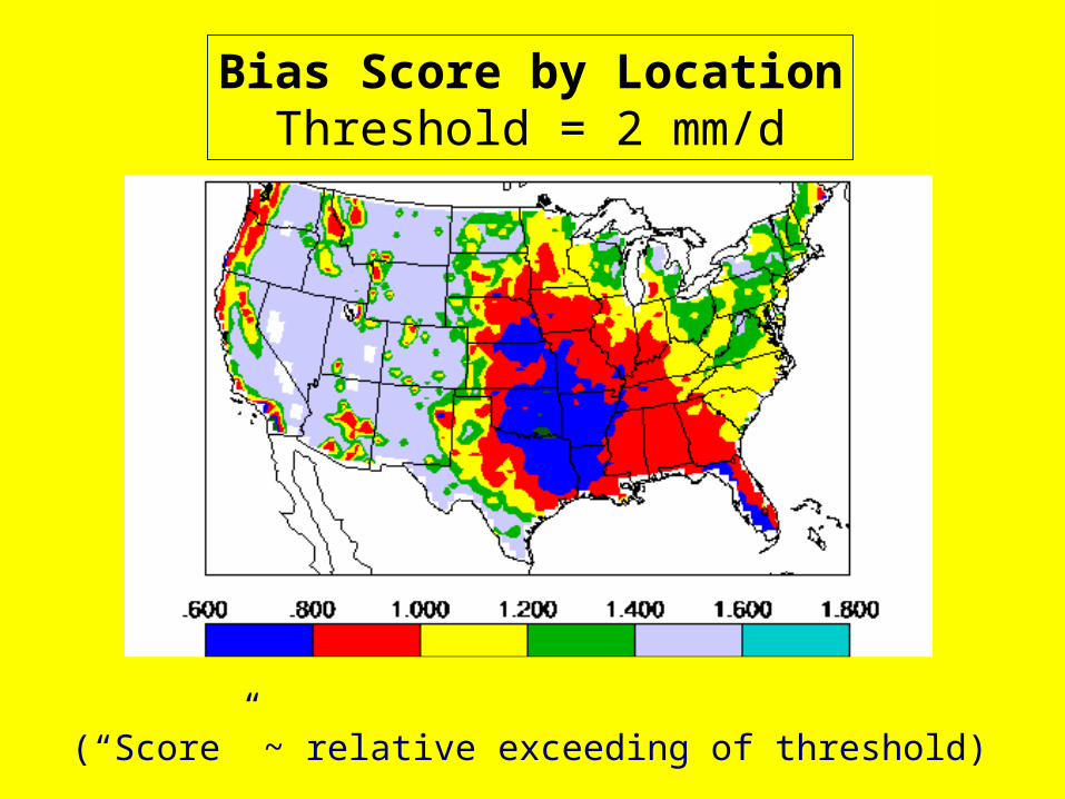
Bias Score by LocationThreshold = 2 mm/d

(“Score” ~ relative exceeding of threshold)
Bias Score by LocationThreshold = 4 mm/d

(“Score” ~ relative exceeding of threshold)
Bias Score by Month~ south-central US ~
SASAS (September 2001)
OutlineOutline
10-yr RCM simulations10-yr RCM simulations
Precipitation analysisPrecipitation analysis
Error evaluationError evaluation
Conclusions: Sources of error?Conclusions: Sources of error?

500 hPa Heights & BiasSep-Oct-Nov
[m]

[m2]
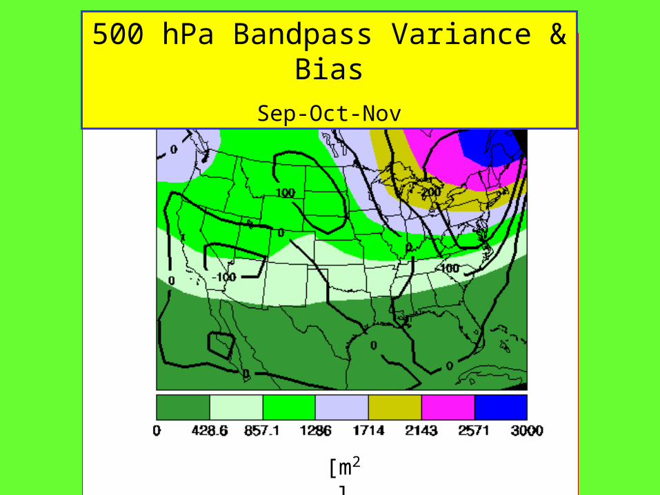
500 hPa Bandpass Variance & Bias
Sep-Oct-Nov

[kg-m-2]
Precipitable Water & Bias
Sep-Oct-Nov

Simulation DomainSimulation Domain

Sep-Oct-Nov 1984
-25
0
25
50
1 31 61 91Time (days)
RegCM2Higgins

Sep-Oct-Nov 1987
-25
0
25
50
1 31 61 91Time [days]
RegCM2
Higgins

Water Balance AnalysisWater Balance Analysis
ΔE =ΔP −(P −E)m +Ro
Observed runoff
Model output
Precipitation error
Evapotranspiration error
From terrestrial balance:
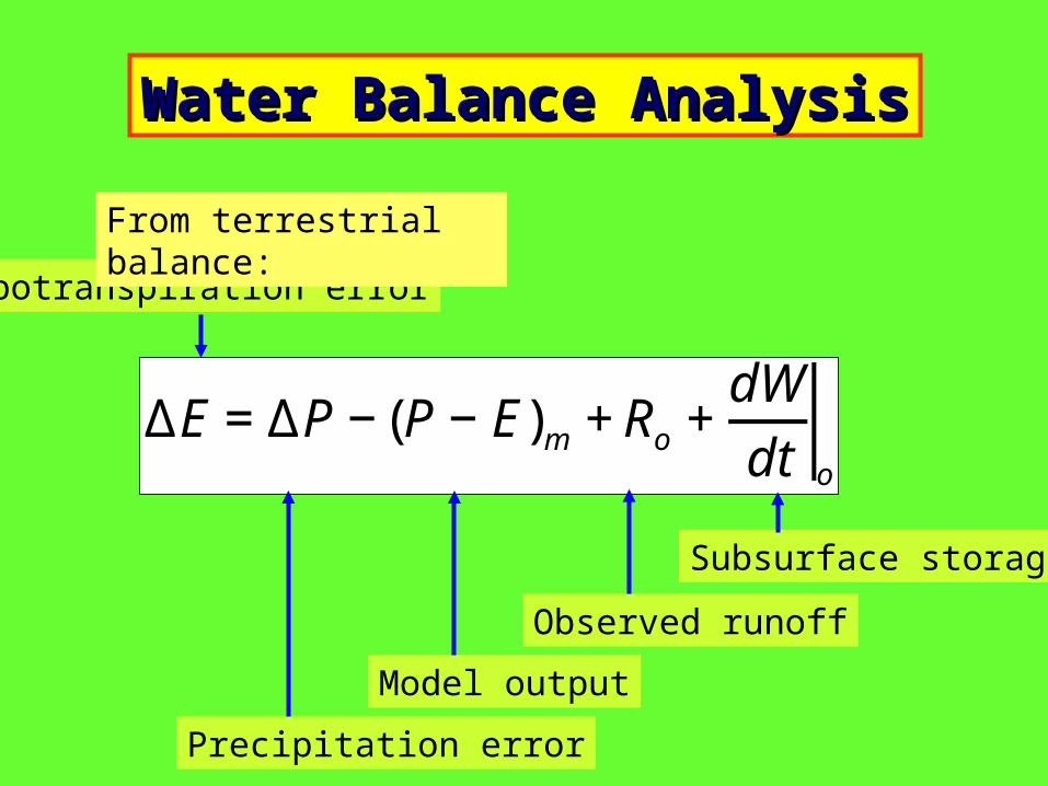
Water Balance AnalysisWater Balance Analysis
ΔE=ΔP −(P −E)m +Ro +dWdt o
Observed runoff
Model output
Precipitation error
Evapotranspiration error
From terrestrial balance:
Subsurface storage

Water Balance AnalysisWater Balance Analysis
ΔC=ΔP −ΔE
Precipitation error
Evapotranspiration error
From atmospheric balance:
Vapor convergence error

Error: Ten-year averageError: Ten-year average
-1.5
-1
-0.5
0
B C DΔ ΔΔP E C
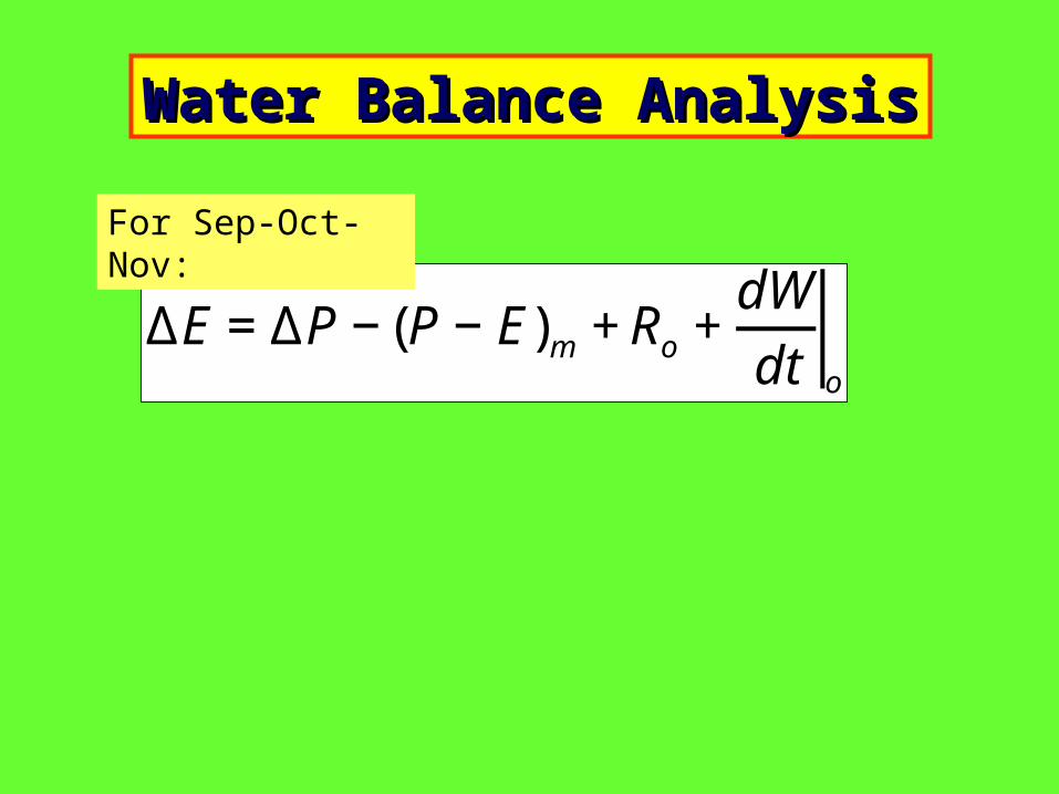
Water Balance AnalysisWater Balance Analysis
ΔE=ΔP −(P −E)m +Ro +dWdt o
For Sep-Oct-Nov:

Water Balance AnalysisWater Balance Analysis
ΔE=ΔP −(P −E)m +Ro +dWdt o
For Sep-Oct-Nov:
Plausible values?• model’s root-zone storage: => -0.5 mm/d• (P-E)m - Ro: => -0.1 mm/d

Error: S-O-N averageError: S-O-N average
-3
-2
-1
0
1
-1 -0.5 0 0.5 1
P E C
Storage [mm/d]
Δ ΔΔP E C
SASAS (September 2001)
OutlineOutline
10-yr RCM simulations10-yr RCM simulations
Precipitation analysisPrecipitation analysis
Error evaluationError evaluation
Conclusions: Sources of error?Conclusions: Sources of error?

SASAS (September 2001)
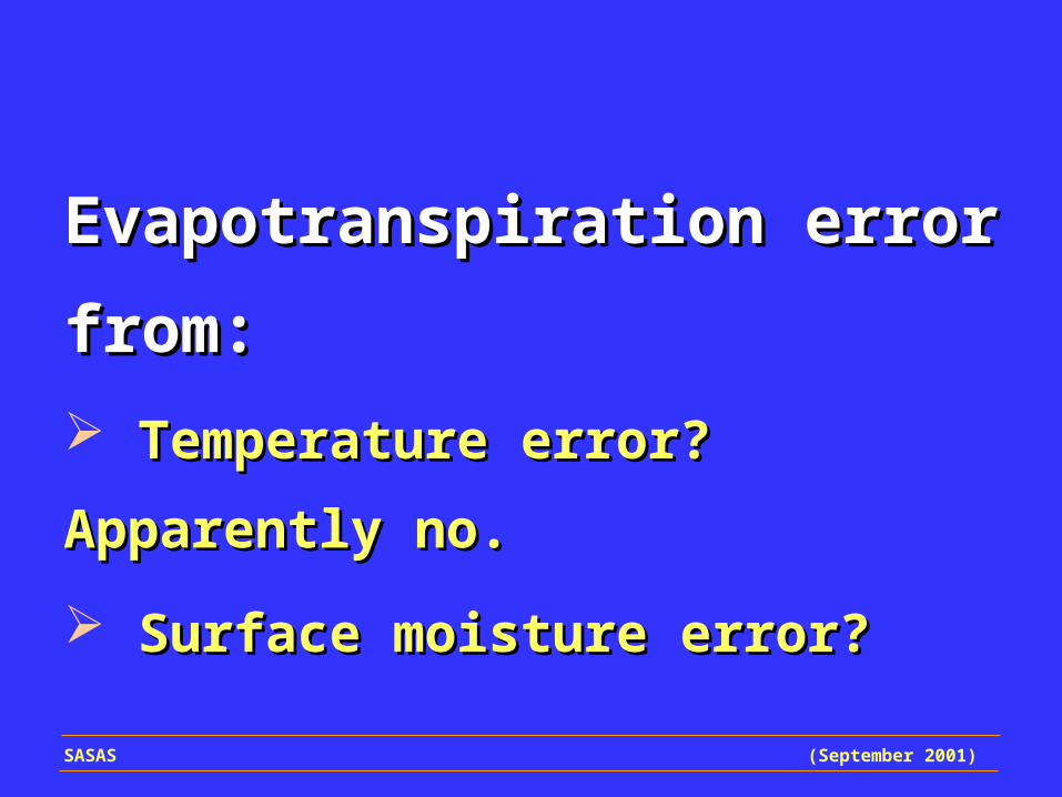
Evapotranspiration error from:Evapotranspiration error from:
Temperature error?Temperature error?
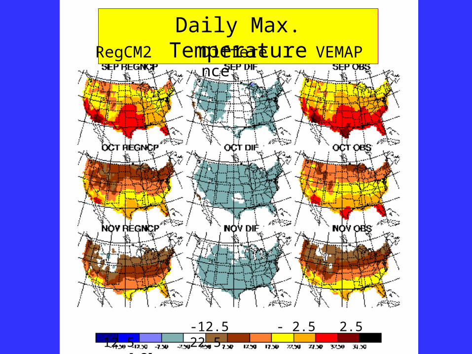
Daily Max. TemperatureRegCM2 Difference VEMAP
-12.5 - 2.5 2.5 12.5 22.5 [oC]

Daily Min. TemperatureRegCM2 Difference VEMAP
-12.5 - 2.5 2.5 12.5 22.5 [oC]
SASAS (September 2001)
Evapotranspiration error from:Evapotranspiration error from:
Temperature error? Apparently no.Temperature error? Apparently no.
Surface moisture error?Surface moisture error?

SASAS (September 2001)
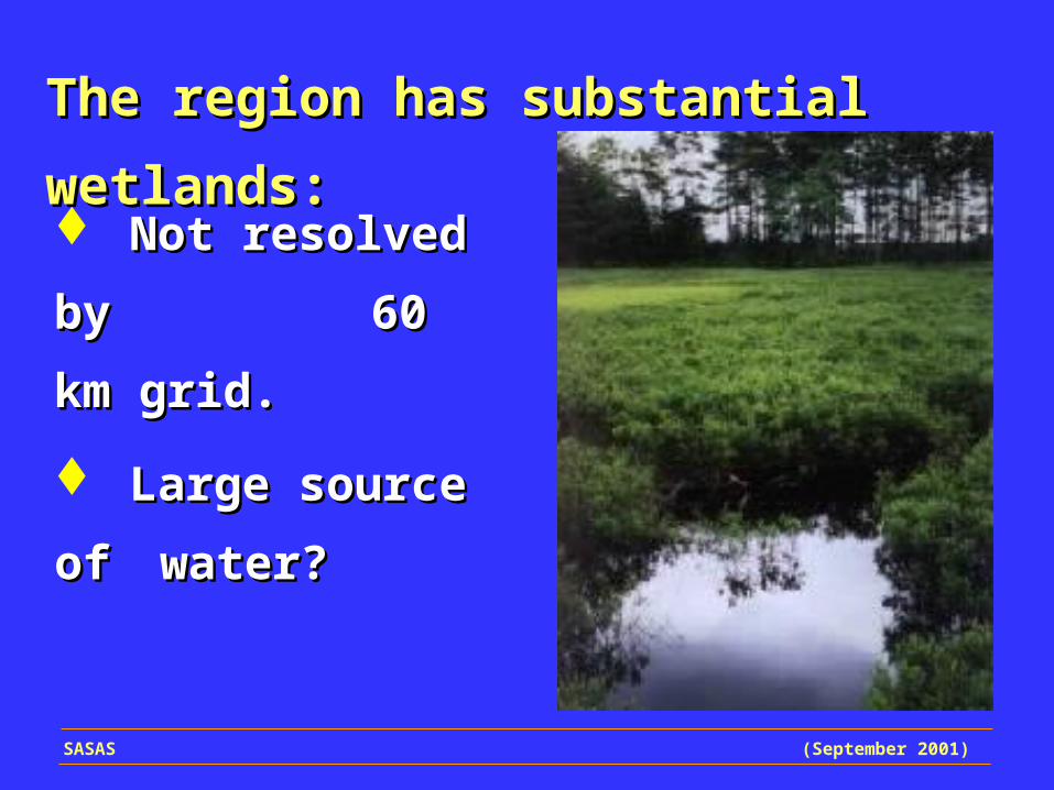
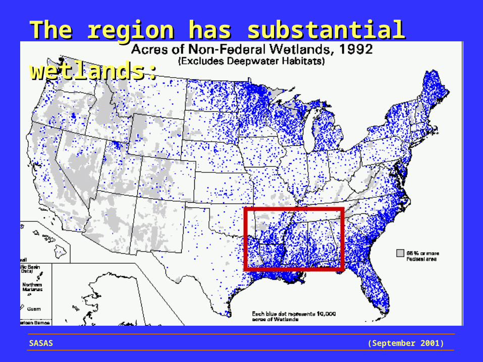
The region has substantial wetlands:The region has substantial wetlands:
SASAS (September 2001)
Not resolved by Not resolved by
60 km grid.60 km grid.
Large source of Large source of
water?water?
The region has substantial wetlands:The region has substantial wetlands:

AcknowledgmentsAcknowledgments
Primary Funding: Primary Funding: U.S. National Oceanic and Atmospheric U.S. National Oceanic and Atmospheric
Administration (NOAA)Administration (NOAA)
Additional Support: Additional Support: Electric Power Research Institute (EPRI)Electric Power Research Institute (EPRI)
SASAS (September 2001)
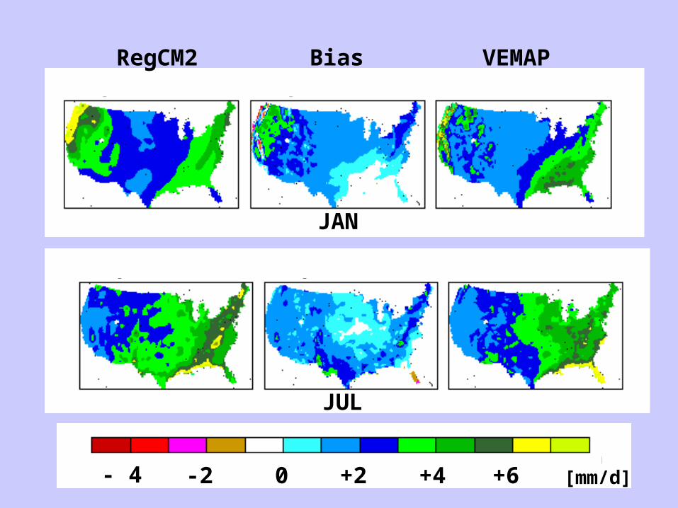
RegCM2 Bias VEMAP
JAN
JUL
0-2 +2 [mm/d]+4 +6- 4


SOM TrajectoriesRegCM
VEMAP
J-J-A

SOM Trajectories
RegCM
D-J-F
VEMAP
D-J-F
RegCM
VEMAP
J-J-A

500 hPa Bandpass Variance &
Bias
(a) Sep-Oct-Nov
(b) Dec-Jan-Feb
[m2]
[m2]
500 hPa Bandpass Variance & Bias
Sep-Oct-Nov

[m]
500 hPa SOM-weighted ave. & bias
October
SASAS (September 2001)
The region has substantial wetlands:The region has substantial wetlands:
SASAS (September 2001)
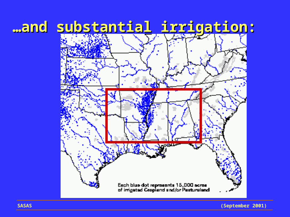
……and substantial irrigation:and substantial irrigation:

SASAS (September 2001)
Hydrological units boundaries:Hydrological units boundaries:
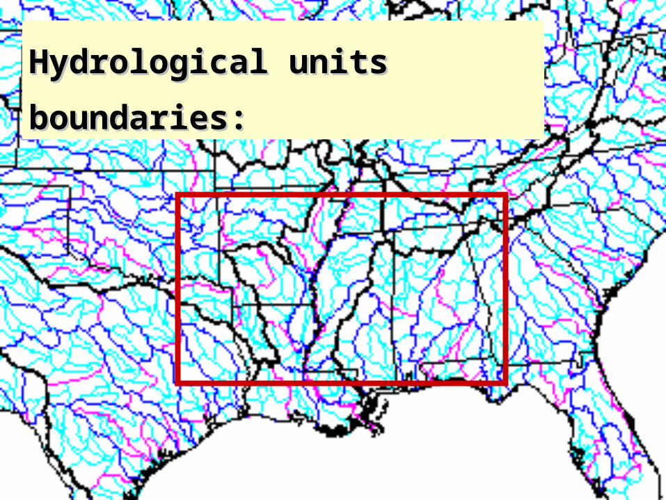
Hydrological units boundaries:Hydrological units boundaries:


![LNAI 4020 - Agent Community Extraction for 2D-RoboSoccer · 2017-08-23 · ior patterns of an individual agent with the help of self-organizing maps (SOMs) is addressed in [9]. We](https://static.fdocuments.in/doc/165x107/5f8f6d4e2767e1393e549013/lnai-4020-agent-community-extraction-for-2d-robosoccer-2017-08-23-ior-patterns.jpg)