Self Organizing Maps: Properties and ApplicationsNeural Computation : Lecture 17

© John A. Bullinaria, 2015

1. The SOM Architecture and Algorithm

2. Properties of the Feature MapApproximation of the Input SpaceTopological OrderingDensity MatchingFeature Selection

3. Applications of Self Organizing Maps

4. Computer Demonstration

L17-2

The Architecture of a Self Organizing Map

We shall concentrate on the popular SOM known as a Kohonen Network. This has afeed-forward structure with a single computational layer of neurons arranged in rowsand columns. Each neuron is fully connected to all the source units in the input layer:

A one dimensional map will just have a single row or column in the computational layer.

Input layer

Computational layer

j

wij

i

L17-3

The SOM Algorithm

The aim is to learn a feature map from the spatially continuous input space, in whichthe input vectors live, to the low dimensional spatially discrete output space, which isformed by arranging the computational neurons into a grid.

The stages of the SOM algorithm that achieves this can be summarised as follows:

1. Initialization – Choose random values for the initial weight vectors wj.

2. Sampling – Draw a sample training input vector x from the input space.

3. Matching – Find the winning neuron I(x) that has weight vector closest to the

input vector, i.e. the minimum value of d j(x) = (xi −wji )2

i=1D

∑ .

4. Updating – Apply the weight update equation Δwji =η(t) Tj,I(x)(t) ( xi − wji )

where Tj,I(x)(t) is a Gaussian neighbourhood and η(t) is the learning rate.

5. Continuation – Keep returning to step 2 until the feature map stops changing.

We shall now explore the properties of the feature map and look at some examples.

L17-4

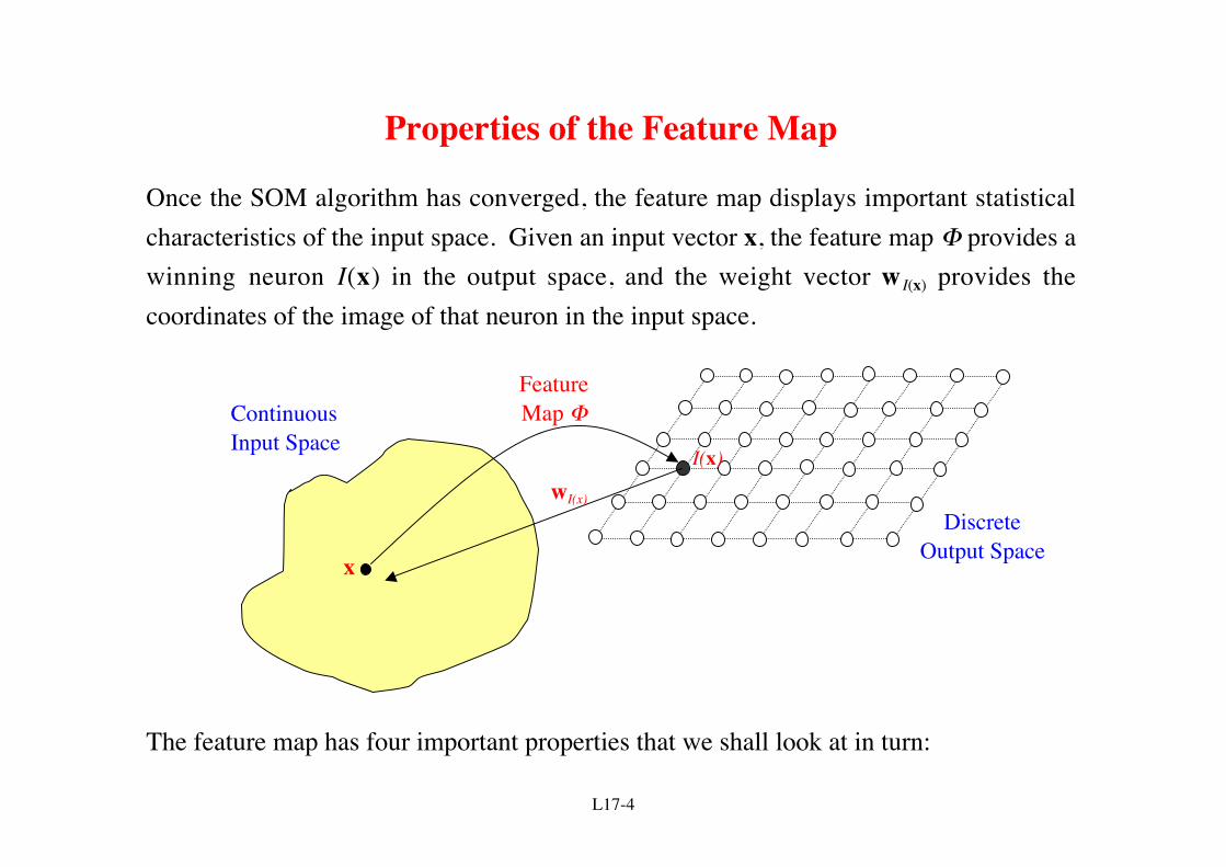
Properties of the Feature Map

Once the SOM algorithm has converged, the feature map displays important statisticalcharacteristics of the input space. Given an input vector x, the feature map Φ provides awinning neuron I(x) in the output space, and the weight vector w I(x) provides thecoordinates of the image of that neuron in the input space.

The feature map has four important properties that we shall look at in turn:

FeatureMap Φ

DiscreteOutput Space

ContinuousInput Space

x

wI(x)

I(x)

L17-5

Property 1 : Approximation of the Input Space

The feature map Φ represented by the set of weight vectors {wi} in the output space,provides a good approximation to the input space.

The aim of the SOM can be stated as the storing of a large set of input vectors {x} byfinding a smaller set of prototypes {w i} that provide a good approximation of theoriginal input space. The theoretical basis of this idea is rooted in vector quantizationtheory, the motivation of which is dimensionality reduction or data compression.

In effect, the goodness of the approximation is given by the total squared distance

D = x − wI (x)x∑

2

which we wish to minimize. If one works through gradient descent style mathematicsto optimize this, we do end up with the SOM weight update algorithm, which confirmsthat it is generating a good approximation to the input space.

L17-6

Property 2 : Topological Ordering

The feature map Φ computed by the SOM algorithm is topologically ordered in thesense that the spatial location of a neuron in the output lattice/grid corresponds to aparticular domain or feature of the input patterns.

The topological ordering property is a direct consequence of the weight update equationthat forces the weight vector wI(x) of the winning neuron I(x) to move toward the inputvector x. The crucial factor is that the weight updates also move the weight vectors wj

of the closest neighbouring neurons j along with the winning neuron I(x). Togetherthese weight changes cause the whole output space to become appropriately ordered.

The feature map Φ can be visualized as an elastic or virtual net with grid like topology.Each output node can be represented in the input space at coordinates given by theirweights. Then, if the neighbouring nodes in output space have their correspondingpoints in input space connected together, the resulting image of the output grid revealsdirectly the topological ordering at each stage of the network training.

L17-7

From: Neural Networks, S. Haykin, Prentice Hill, 1999.

L17-8

From: Neural Networks, S. Haykin, Prentice Hill, 1999.

L17-9

From: Introduction to the Theory of Neural Computation,Hertz, Krogh & Palmer, Addison-Wesley, 1991.

L17-10

From: Introduction to the Theory of Neural Computation,Hertz, Krogh & Palmer, Addison-Wesley, 1991.

L17-11

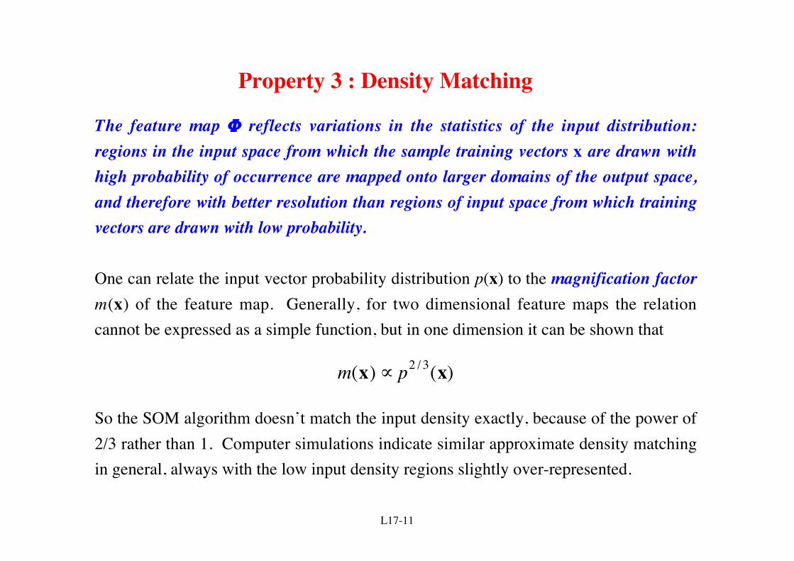
Property 3 : Density Matching

The feature map Φ reflects variations in the statistics of the input distribution:regions in the input space from which the sample training vectors x are drawn withhigh probability of occurrence are mapped onto larger domains of the output space,and therefore with better resolution than regions of input space from which trainingvectors are drawn with low probability.

One can relate the input vector probability distribution p(x) to the magnification factorm(x) of the feature map. Generally, for two dimensional feature maps the relationcannot be expressed as a simple function, but in one dimension it can be shown that

m(x) ∝ p2 / 3(x)

So the SOM algorithm doesn’t match the input density exactly, because of the power of2/3 rather than 1. Computer simulations indicate similar approximate density matchingin general, always with the low input density regions slightly over-represented.

L17-12

Property 4 : Feature Selection

Given data from an input space with a non-linear distribution, the self organizing mapis able to select a set of best features for approximating the underlying distribution.

This property is a natural culmination of the preceding three properties.

Remember how Principal Component Analysis (PCA) is able to compute the inputdimensions which carry the most variance in the training data. It does this by computingthe eigenvectors associated with the largest eigenvalues of the correlation matrix.

PCA is fine if the data really does form a line or plane in input space, but if the dataforms a curved line or surface (e.g. a semi-circle), linear PCA is no good, but a SOM willovercome the approximation problem by virtue of its topological ordering property.

The SOM provides a discrete approximation of finding so-called principal curves orprincipal surfaces, and may therefore be viewed as a non-linear generalization of PCA.

L17-13

Application: World Poverty Map

Inputs are 39 indicators like health, nutrition, education, etc. for each country. Output:

L17-14

More details at: http://www.cis.hut.fi/research/som-research/worldmap.html

L17-15

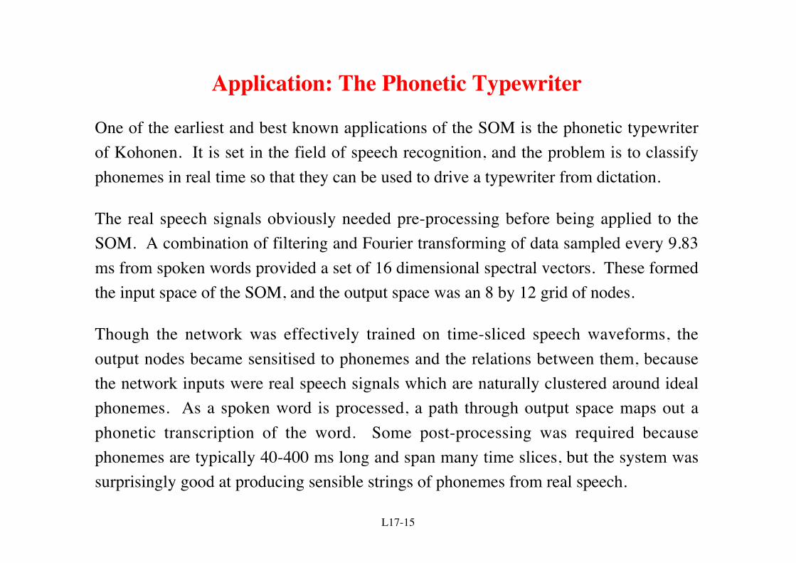
Application: The Phonetic Typewriter

One of the earliest and best known applications of the SOM is the phonetic typewriterof Kohonen. It is set in the field of speech recognition, and the problem is to classifyphonemes in real time so that they can be used to drive a typewriter from dictation.

The real speech signals obviously needed pre-processing before being applied to theSOM. A combination of filtering and Fourier transforming of data sampled every 9.83ms from spoken words provided a set of 16 dimensional spectral vectors. These formedthe input space of the SOM, and the output space was an 8 by 12 grid of nodes.

Though the network was effectively trained on time-sliced speech waveforms, theoutput nodes became sensitised to phonemes and the relations between them, becausethe network inputs were real speech signals which are naturally clustered around idealphonemes. As a spoken word is processed, a path through output space maps out aphonetic transcription of the word. Some post-processing was required becausephonemes are typically 40-400 ms long and span many time slices, but the system wassurprisingly good at producing sensible strings of phonemes from real speech.

L17-16

Overview and Reading

1. We began by reviewing the SOM architecture and algorithm.2. Then we considered the important properties of the feature map: its

ability to approximate the input space, the topological ordering thatemerges, the matching of the input space probability densities, and theability to select the best set of features for approximating the under-lying input distribution.

3. We ended by looking at some simple applications.

Reading

1. Haykin-2009: Sections 9.3, 9.4, 9.5, 9.62. Beale & Jackson: Sections 5.2, 5.3, 5.4, 5.5, 5.73. Gurney: Sections 8.1, 8.2, 8.34. Hertz, Krogh & Palmer: Sections 9.4, 9.55. Callan: Sections 3.1, 3.2, 3.3, 3.4, 3.5