"Self fulfilling Debt Crises, Revisited: The Art of the Desperate Deal", by Mark Aguiar, Satyajit...
35
Self-Fulfilling Debt Crises, Revisited: The Art of the Desperate Deal Mark Aguiar Satyajit Chatterjee Harold L. Cole Zachary Stangebye September 2, 2016 1 / 29
-
Upload
ademuproject -
Category
Economy & Finance
-
view
80 -
download
0
Transcript of "Self fulfilling Debt Crises, Revisited: The Art of the Desperate Deal", by Mark Aguiar, Satyajit...

Self-Fulfilling Debt Crises, Revisited: TheArt of the Desperate Deal
Mark Aguiar Satyajit Chatterjee
Harold L. Cole Zachary Stangebye
September 2, 2016
1 / 29

Desperate Deals
I What does a sovereign do when faced with the prospect of afailed auction?
I In Cole-Kehoe they default
I In practice, they look for alternative financing
I Often tolerating high spreads.
I Occasionally ending up defaulting.
2 / 29

Desperate Deals
I What does a sovereign do when faced with the prospect of afailed auction?
I In Cole-Kehoe they default
I In practice, they look for alternative financing
I Often tolerating high spreads.
I Occasionally ending up defaulting.
2 / 29

Portugal
I Difficulty in raising funds through auctions starting in 2011
I Private placement of bonds in January 2011 (reported aspurchased by China)
I Official ¤78 billion package in May 2011I ¤34.2 billion dispersed in 2011 and ¤28.5 in 2012
I Dual auction in October 2012I Bought “September 2013” bonds
I Sold “October 2015” bonds
I Goal: Clear “space” for auctions in 2013/2014
I Launched new issue in early 2013
3 / 29
Self-Fulfilling Debt Crises, Revisited
I What is a self-fulfilling debt crisis?
I Cole-Kehoe: Failed auction today generates default today
I Zero price for any amount of bonds issued
I Choose to default - hence self-fulfilling.
I Our model generates less extreme rollover crises than in C-K.
I Keeps C-K’s “static” rollover-crisis multiplicity but considers aricher notion of “failed” auctions.
I Generate spikes in spreads without defaults, like the data.
I Our model has some surprising welfare implications.(Buybacks not all bad.)
4 / 29

FrameworkEndowment: Stochastic Growth as in Aguiar-Gopinath
I Small open economy
I Discrete time
I Markov process for endowment growth
yt ≡ lnYt =t∑
s=0
gs + zt
= yt−1 + gt + zt − zt−1
I gt follows an AR(1) process and zt is iid
5 / 29
FrameworkBonds: Random Maturity as in Chatterjee-Eyigungor
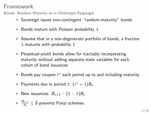
I Sovereign issues non-contingent “random-maturity” bonds
I Bonds mature with Poisson probability λ
I Assume that in a non-degenerate portfolio of bonds, a fractionλ matures with probability 1
I Perpetual-youth bonds allow for tractably incorporatingmaturity without adding separate state variables for eachcohort of bond issuances
I Bonds pay coupon r∗ each period up to and including maturity
I Payments due in period t: (r∗ + λ)Bt
I New issuances: Bt+1 − (1− λ)Bt
I Bt+1
Yt≤ b̄ prevents Ponzi schemes.
6 / 29

FrameworkLenders
I Risk averse OLG lenders (risk aversion not conceptuallyimportant)
I Financial markets are segmented: Finite wealth available toparticipate in bond market
I Tractability: Period t’s set of investors hold bonds for oneperiod and then sell them to a new cohort of investors at startof t + 1
7 / 29

TimingModification of Cole-Kehoe
Initial State:s
AuctionB ′ − (1− λ)B
at priceq(s,B ′)
Settlement
No Default
Default
V R(s,B ′)
VD(s)
Next Pe-riod: s ′
8 / 29

Settlement
I Auction Revenue:
x(s,B ′) ≡ max{q(s,B ′)(B ′ − (1− λ)B), 0
}I Proceeds from auction are held in escrow until government
makes repayment decision
I If government repays, can draw on settlement funds forrepayment and consumption
I If government defaults, auction revenue disbursed tobondholders in proportion to face value of claims:
RD(s,B ′) =x(s,B ′)
B ′ + (r∗ + λ)B
I If B ′ < (1− λ)B: Buyback funds are paid out and gone.
9 / 29

Settlement
I No Default:
I Old lenders receive (r∗ + λ)B
I New lenders hold B ′ into next period
I Default:
I Old lenders receive RD(s,B ′)(r∗ + λ)B
I New lenders receive RD(s,B ′)B ′
10 / 29

The Government’s ProblemPreferences
I Sovereign government makes all consumption-savings-defaultdecisions
I Sovereign’s preferences over sequence of aggregateconsumption {Ct}∞t=0:
E∞∑t=0
βtu(Ct)
with
u(C ) =C 1−σ
1− σ
11 / 29

Value Functions
I V (s) denotes start-of-period value of government
I V R(s,B ′) denotes value if having auctioned B ′ − (1− λ)Bthe government decides to repay (r∗ + λ)B at settlement
I VD(s) denotes the value of defaulting at settlement(independent of amount auctioned) ⇒ lose fraction φ ofendowment until “redemption” from default status
I Strategic default implies:
V (s) = max
⟨max
B′≤b̄YV R(s,B ′),VD(s)
⟩
12 / 29

Bellman Equations
I If repay...
V R(s,B ′) = u(C ) + βE[V (s ′)|s,B ′
],
with
C = Y + q(s, b′)(B ′ − (1− λ)B)− (r∗ + λ)B.
I If default...
VD(s) = u(Y D) + βEV E (s ′)
V E (s) = u((1− φ)Y ) + β(1− ξ)E[V E (s ′)
∣∣∣∣s]+ βξE
[V (s ′)
∣∣∣∣s,B ′ = 0
]
13 / 29

Equilibrium
I Markov Equilibrium
I States s ∈ S elements of s are:I Endowment: (Y , g , z)
I Bonds: B
I Beliefs: ρ
I Policy Functions:
I Bond-issuance: B(s)
I Default: D(s, b′) ∈ [0, 1]
I Bond-demand: µ∗(s, b′)
I Price function: q(s,B ′) ∈ [0, 1]
I Market clearing: µ∗(s,B ′)W = q(s,B ′)B ′.
14 / 29

Multiplicity of Equilibria
I There is a “static” multiplicity in a given period
I Arises because of timing convention: Failed auction even forsmall levels of bond issuances can be supported in equilibrium
I Suppose the continuation equilibrium is held constant and weconsider alternative price schedules for the current period’sauction
I Consider two scenarios for today’s auction, holding constantequilibrium behavior going forward
15 / 29

Cole-Kehoe Crisis
I Zero price for any B ′ ≥ (1− λ)B:
V R(s, (1− λ)B)
= u (Y − (r∗ + λ)B) + βE[V (s ′)|s,B ′ = (1− λ)B
]< VD(s).
Non-Crisis
I A pair (q̃, B̃) such that:
V R(s,B ′) =
u(Y − (r∗ + λ)B + q̃[B̃ − (1− λ)B]
)+ βE
[V (s ′)|s, B̃
]> VD(s).
16 / 29

Constructing Equilibria
I For a given state s and equilibrium policy functions, we canprice a bond conditional on no-default at settlement thisperiod
I Such within-period commitment is the assumption ofEaton-Gersovitz models
I Our exercise assumes only commit for the current period, andthen no commitment going forward
I Let qEG (s,B ′) denote this price
17 / 29

Crisis Zone
I Define a “Crisis Zone” by evaluating V R(s,B ′) under qEG :
C ≡{s ∈ S
∣∣∣∣ maxB′≤(1−λ)B
V R(s,B ′) ≤ VD(s) &
maxB′≥(1−λ)B
V R(s,B ′) ≥ VD(s)
}.
I This set identifies states in which:I Faced with qEG , the government would have no reason to
default
I Faced with q = 0 for B ′ > (1− λ)B, it will default
I Crisis zone combination of high B and low (Y , g , z)
18 / 29

Self-Fulfilling Crises
I In Cole-Kehoe equilibrium, a rollover crisis is an equilibrium inwhich prices are zero for any positive amount of debt issuance
I We relax this and consider a broader set of crisis equilibria
I Build on the mixed strategy equilibria of Aguiar and Amador(2014)
I That model had potential buybacks and randomization off theequilibrium path
I We now bring this onto the equilibrium path and consider crisisissuances
19 / 29

Desperate DealsRethinking Failed Auctions
Desperate Deal Price Schedule: An Indifference Condition
qD(s,B ′) =
{q̃
∣∣∣∣VD(s) = u(Y − (r∗ + λ)B + q̃[B ′ − (1− λ)B]
)+ βE
[V (s ′)|s,B ′
]}.
I Support as mixed-strategy equilibrium with appropriate choiceof D(s,B ′) ∈ [0, 1]
I Feasible for 0 ≤ qD(s,B ′) ≤ qEG (s,B ′)
I Government indifferent over feasible B ′ so make selection.
20 / 29

Crisis Price Schedule
0.0 0.2 0.4 0.6 0.8 1.0 1.20.0
0.1
0.2
0.3
0.4
0.5
0.6
0.7
0.8
0.9
1.0
B0
Y
qD
qEG
I Desperate deals (indifference) prices in black. EG (good)prices in red. CK price is 0 for issuances.
21 / 29

Evolution of Beliefs
I iid probability of crisis if s ∈ CI q = qD
I Assume B(s) = B ′/Y = B ′−1/Y−1 (prior debt-output ratioequals new ratio)
I Contrast with “No Desperate Deals” modelI Just original Cole-Kehoe Eq.
I q = 0 for any positive issuance in a crisis
22 / 29

CalibrationPre-Set Parameters
I Calibrate endowment to Mexico 1980Q1-2001Q4
I Set risk aversion coefficient for sovereign and lenders at 2
I Set quarterly risk free rate to 1%
I Set average maturity to 8 quarters
I Set average exclusion to 8 quarters
I Probability ρ = rC is 14
23 / 29

The Role of Desperate Deals
Target Moment Data Benchmark No Deals
BY 65.6% 66.6% 64.5%r − r∗ 3.4% 3.4% 3.4%σ(r − r∗) 2.5% 2.5% 0.1 %Default Freq 2.0% 2.0% 2.1%
I Massive increase in volatility relative to No Deals(and without deterministic growth, nonlinear default costs andvolatility output).
I Lower debt level with No Deals reduces difference in defaults.(Desperate deals reduces borrowing discipline.)
24 / 29

Crises and Default
I Crises:I Fraction of quarters in crisis zone: 8.0%
I Rollover crises occur 2% of the time
I Defaults:I Default rate 2% per annum (targeted)
I 97% of defaults coincide with negative growth
I 70% of defaults coincide with rollover crisis
I Conditional on rollover crisis, default on average 15% of time
25 / 29

Distribution of r − r ∗
Conditional on CrisisFr
eque
ncy
0 .1 .2 .3 .4Spread
Default Unrealized Default Realized
26 / 29

Equilibrium Price ScheduleWith and Without Crisis Issuances
0.0 0.1 0.2 0.3 0.4 0.5 0.6 0.7 0.8 0.9 1.00.0
0.1
0.2
0.3
0.4
0.5
0.6
0.7
0.8
0.9
1.0
B0
Y
q
BenchmarkNo Deals
I Better price schedule from lenders’ anticipation of bettertreatment with desperate deals.
27 / 29

Welfare Resultssome surprises
I Desperate Deals equilibrium slightly dominates No DealsI Prices better conditional on crisis
I Government captures this through ex ante price schedule
I Off-setting effect: Higher debt and more defaults due to morefavorable spreads
I Buybacks during rollover crises raises welfareI Counters Bulow-Rogoff’s Buyback Boondoggle
28 / 29

Conclusion
I Models based upon Eaton-Gersovitz environment strugglewith matching spread volatility.
I Cole-Kehoe environment also generates limited volatility inspreads and extreme outcome conditional on a crisis
I In our approach, self-fulfilling crises generate a mixture offundamental and belief-driven defaults, and desperate deals
I Crises now look more like what we see in the data.
I Extreme spreads look like we see in the data.
I Interesting welfare implications (relative to classicBulow-Rogoff).
29 / 29


![Satyajit Ray - Patol Babu Filmstar[1]](https://static.fdocuments.in/doc/165x107/577d1f321a28ab4e1e901430/satyajit-ray-patol-babu-filmstar1.jpg)