Self-Calibration and Metric Reconstruction in spite of Varying and

International Journal of Computer Vision, ?, 1?? (1998)c

1998 Kluwer Academic Publishers, Boston. Manufactured in The Netherlands.

Self-Calibration and Metric Reconstructionin spite of Varying and Unknown Intrinsic Camera Parameters

MARC POLLEFEYS, REINHARD KOCH AND LUC VAN GOOLESAT-PSI, K.U.Leuven, Kardinaal Mercierlaan 94, B-3001 Heverlee, Belgium

[email protected]@[email protected]

Received April, 1998; Revised May, 1998

Abstract. In this paper the theoretical and practical feasibility of self-calibration in the presence of varyingintrinsic camera parameters is under investigation. The paper’s main contribution is to propose a self-calibrationmethod which efficiently deals with all kinds of constraints on the intrinsic camera parameters. Within thisframework a practical method is proposed which can retrieve metric reconstruction from image sequences obtainedwith uncalibrated zooming/focusing cameras. The feasibility of the approach is illustrated on real and syntheticexamples. Besides this a theoretical proof is given which shows that the absence of skew in the image plane issufficient to allow for self-calibration. A counting argument is developed which –depending on the set of constraints–gives the minimum sequence length for self-calibration and a method to detect critical motion sequences is proposed.

1. Introduction

In recent years, researchers have been studying self-calibration methods for cameras. Mostly completelyunknown but constant intrinsic camera parameterswere assumed. This has the disadvantage that the zoomcan not be used and even focusing is prohibited. Onthe other hand, the proposed perspective model is oftentoo general compared to the range of existing cameras.Mostly the image axes can be assumed orthogonal andoften the aspect ratio is known. Therefore a tradeoffcan be made and by assuming these parameters to beknown, one can allow (some of) the other parametersto vary throughout the image sequence.

Since it became clear that projective reconstruc-tions could be obtained from image sequencesalone (Faugeras, 1992, Hartley, 1992), researcherstried to find ways to upgrade these reconstructions tometric (i.e. Euclidean up to unknown scale). Manymethods were developed which assumed constant in-trinsic camera parameters. Most of these methods

are based on the absolute conic which is the onlyconic which stays fixed under all Euclidean transfor-mations (Semple and Kneebone, 1952). This coniclays in the plane at infinity and its image is directlyrelated to the intrinsic camera parameters, hence theadvantage for self-calibration.

Faugeras et al. (1992), see also (Luong and Faugeras,1997), proposed to use the Kruppa equations whichenforce that the planes through two camera centerswhich are tangent to the absolute conic should alsobe tangent to both of its images. Later on Zeller andFaugeras (1996) proposed a more robust version of thismethod.

Heyden and Astrom (1996), Triggs (1997) andPollefeys and Van Gool (1997b) use explicit constraintswhich relate the absolute conic to its images. Theseformulations are especially interesting since they caneasily be extended to deal with varying intrinsic cameraparameters.

Pollefeys and Van Gool (1997a) also proposed astratified approach which consists of first locating theplane at infinity using the modulus constraint (i.e. for

2 Pollefeys, et al.

constant intrinsic camera parameters the infinity ho-mography should be conjugated to a rotation matrix)and then calculating the absolute conic. Hartley (1993)proposed another approach based on the minimizationof the difference between the intrinsic camera param-eters for the different views.

So far not much work has been done on varying in-trinsic camera parameters. Pollefeys et al. (1996) alsoproposed a stratified approach for the case of a varyingfocal length, but this method required a pure trans-lation as initialization, along the lines of Armstronget al. (1994) earlier account for fixed intrinsic cam-era parameters. Recently Heyden and Astrom (1997)proved that self-calibration was possible when the as-pect ratio was known and no skew was present. Theself-calibration method proposed in their paper is basedon bundle adjustment which requires non-linear min-imization over all reconstructed points and camerassimultaneously. No method was proposed to obtain asuitable initialization.

In this paper their proof is extended. It will be shownthat the absence of skew alone is enough to allow self-calibration. A versatile self-calibration method is pro-posed which can deal with varying types of constraints.This will then be specialized towards the case where thefocal length varies, possibly also the principal point.

Section 2 of this paper introduces notations and somebasic principles, Section 3 gives a counting argumentfor self-calibration and finally shows that imposing theabsence of skew is sufficient to restrict the projectiveambiguity to the group of similarities (i.e. metric self-calibration). In Section 4 the actual method is devel-oped. A simplified linear version is also given whichcan be used for initialization. Section 5 summarizesthe complete procedure for metric reconstruction ofarbitrarily shaped, rigid objects from an uncalibratedimage sequence alone. The method is then validatedthrough the experiments of Section 6, in Section 7some more results illustrate the flexibility of our ap-proach. Section 8 concludes this paper and gives somedirections for further research.

2. Notations and basic principles

In this section the basic principles and notations usedin this paper are introduced. Projective geometry andhomogeneous coordinates are used. Metric entities areindicated with a subscript .

2.1. Cameras

The following equation is used to describe the perspec-tive projection of the scene onto the images (1)

where is a projection matrix describing theperspective projection process, and ! " are vectors containing the homogeneouscoordinates of the world points respectively imagepoints. Notice that will be used throughout thispaper to indicate equality up to a non-zero scale factor.

In the metric case the camera projection matrix fac-torizes as follows:$#%&' (*) - (,+- (2)

Here . (/0+01 denotes a rigid transformation (i.e. ( is arotation matrix and + is a translation vector) which in-dicate the position and orientation of the camera, whilethe upper triangular calibration matrix & encodes theintrinsic parameters of the camera:& 23547698;:<647=>:?= @A (3)

where4 6

and4 =

represent the focal length divided bythe pixel width resp. height, . :B6 / :<= 1 represents theprincipal point and

8is a factor which is zero in the

absence of skew.

2.2. Conics and Quadrics

In this paper a specific conic and quadric play an im-portant role. Therefore some related notations are in-troduced here. A conic is represented by a C sym-metric matrix D , a quadric by a EF symmetric matrixG

. A point on the conic satisfies H D IKJ anda point on the quadric satisfies G LJ . Adual (or line) conic is represented by a MN matrixDO , while a dual (or plane) quadric is represented bya PN matrix

G O . A line Q tangent to the conic Dsatisfies Q DROSQ TJ . A plane U tangent to the quadricG

satisfies U G OU TJ . Provided D resp.G

are fullrank DRO DWVYX and

G O G VBX . It can be shownthat (Karl et al., 1994),D O G O [Z (4)

This equation describes the projection of the outline ofa dual quadric onto a dual image conic.

Self-Calibration and Metric Reconstruction 3

2.3. Transformations

A projective transformation of 3D space is describedby a , matrix \ . In the case of a similarity trans-formation \ # takes on the following form:\ #%^]Y_ ( +J F` (5)

with _ a global scale factor ( _ yields a Euclideantransformation).

Points, planes and projection matrices are trans-formed as follow:9a \ K/ U a \ V U and >a^ \ VBX Z (6)

On quadrics and dual quadrics the effect of a projectivetransformation is as follows:G a \ V G \ VYX and

G O a \ G O \ [Z (7)

3. Some theory

Before developing a practical self-calibration algo-rithm some theoretical aspects of the problem are stud-ied in this section. First a counting argument is givenwhich states the minimal sequence length that allowsself-calibration from a specific set of constraints. Thena proof is given that self-calibration is possible for theminimal case where the only available constraint is theabsence of skew.

3.1. A counting argument

To restrict the projective ambiguity (15 degrees of free-dom) to a metric one (3 degrees of freedom for rotation,3 for translation and 1 for scale), at least 8 constraintsare needed. This thus determines the minimum lengthof a sequence from which self-calibration can be ob-tained, depending on the type of constraints which areavailable for each view. Knowing an intrinsic cameraparameter for b views gives b constraints, fixing oneyields only bc constraints.bN.edfgbYhjiFb 1lk .mbc j1 .-d 4<n <oqpg1ErtsOf course this counting argument is only valid for non-critical motion sequences (see Section 4.3).

Therefore the absence of skew (1 additional con-straint per view) should in general be enough to allowself-calibration on a sequence of 8 or more images. InSection 3.2 it will be shown that this simple constraint

is not bound to be degenerate. If in addition the aspectratio is known (e.g.

4u6 47= ) then 4 views should besufficient. When also the principal point is known, apair of images is enough. A few more examples aregiven in Table 1.

3.2. Self-calibration using only the absence of skew

In this paragraph it is shown that the absence of skewcan be sufficient to yield a metric reconstruction. Thisis an extension of the theorem proposed by Heydenand Astrom (1997) which besides orthogonality alsorequires the aspect ratio to be known.

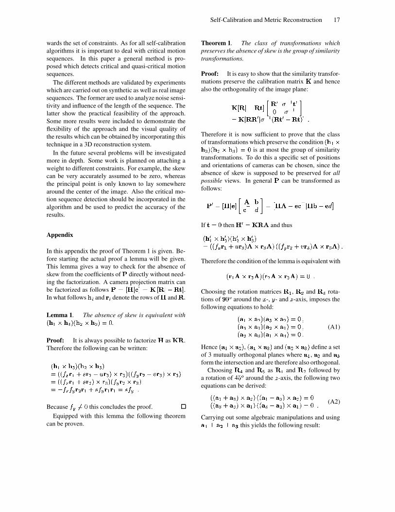
Theorem 1. The class of transformations whichpreserves the absence of skew is the group of similaritytransformations.

The proof is given in the appendix. If a sequence isgeneral enough (in its motion) it follows from this the-orem that only a projective representation of the cam-eras which can be related to the original ones througha similarity transformation (possibly including a mir-roring) would satisfy the orthogonality of rows andcolumns for all views. Using oriented projective ge-ometry (Laveau and Faugeras, 1996) the mirroringambiguity can easily be eliminated. Therefore self-calibration and metric reconstruction is possible usingthis orthogonality constraint only.

Of course adding more constraints will yield morerobust results and will diminish the probability of en-countering critical motion sequences.

4. Self-Calibration

It is a well-known result that from image correspon-dences alone the camera projection matrices and thereconstruction of the scene points can be retrieved upto a projective transformation (Faugeras, 1992, Hart-ley, 1992). Note that without additional constraintsnothing more can be achieved. This can be seen fromthe following equation.9 . \ VBX 1 .m\ >1vw$xyzxwith \ an arbitrary projective transformation. There-fore . x / x 1 is also a valid reconstruction from theimage points .

4 Pollefeys, et al.

Table 1. A few examples of minimum sequence length required to allow self-calibrationconstraints known fixed min #imagesno skew | fixed aspect ratio and absence of skew | ~-~ known aspect ratio and absence of skew | , ~ ~ only focal length is unknown | , ~ ~ , , standard self-calibration problem , , , , |

In general, however, some additional constraints areavailable. Some intrinsic parameters are known or canbe assumed constant. This yields constraints whichshould be verified when is factorized as in Eq. (2).

It was shown that when no skew is present, the am-biguity of the reconstruction can be restricted to metric(see Section 3.2). Although this is theoretically suffi-cient, under practical circumstances often much moreconstraints are available and should be used.

In Euclidean space two entities are invariant –setwise, not pointwise– under rigid transformations.The first one is the plane at infinity which allowsto compute affine measurements. The second entity isthe absolute conic which is embedded in the plane atinfinity. If besides the plane at infinity the absoluteconic has also been localized, metric measurementsare possible.

When looking at a static scene from different view-points the relative position of the camera towards and is invariant. If the motion is general enough,only one conic in one specific plane will satisfy thiscondition. The absolute conic can therefore be used asa virtual calibration pattern which is always present inthe scene.

A practical way to encode both the absolute conic and the plane at infinity " is through the use ofthe absolute quadric FO (Semple and Kneebone, 1952)(introduced in computer vision by Triggs (1997), seealso Heyden and Astrom, (1996), Pollefeys and VanGool (1997b). This dual quadric consists of planestangent to the absolute conic. Its null-space is theplane at infinity. In a metric frame it is represented

by a CP symmetric rank 3 matrix O# ] JJJ ` .

Using (5) and (7) it can be verified that for a similaritytransformation \ # O# \ # O# . Similar to (4) theprojection of the absolute quadric in the image yieldsthe dual image absolute conic: O w& & O (8)

independent of the chosen projective basis. UsingEq. (2) this can be verified for a metric basis. Through

Eqs. (6) and (7), Eq. (8) can then be verified for anyprojective basis. Some of these concepts are illustratedin Figure 1.

Therefore constraints on the intrinsic camera pa-rameters in & can be translated to constraints on theabsolute quadric. If enough constraints are at handonly one quadric will satisfy them all, i.e. the absolutequadric. At that point the scene can be transformedto the metric frame (which brings FO to its canonicalform).

4.1. Non-linear Approach

Eq. (8) can be used to obtain the metric calibration fromthe projective one. The dual image absolute conics !Oshould be parameterized in such a way that they en-force the constraints on the calibration parameters. Forthe absolute quadric O a minimum parameterization(8 parameters) should be used. This can be done byputting FO and by calculating FO from the rank3 constraint. The following parametrization satisfiesthese requirements: O ^] &P& c &P& c &P& &P& ` Z (9)

iΚΚ

ω

C

Π

i

∗

ωi

Ω(ω,Π )

T

οοοο

Fig. 1. The absolute quadric which encodes both the planeat infinity (affine reference entity) and the absolute conic ¡(metric reference entity), projects to the dual image of the absoluteconic ¡£¢5¤w¥¢¦¥$§¢ . The projection equation allows to translateconstraints on the intrinsic parameters to constraints on .


Here defines the position of the plane at infinity¨ © . In this case the transformation fromprojective to metric is particularly simple:

\ª« #%¬] & VBX J ` (10)

An approximate solution to these equations can be ob-tained through non-linear least squares. The followingcriterion should be minimized:R®°¯[±² °³ X

´´´´ & & µ & & µS¶ c !O µ O µ¶ ´´´´¸·¶ Z (11)

Remark that to obtain meaningful results & & and !O should both be normalized to have Frobeniusnorms equal to one.

If one chooses X ¹ ) º» , Eq. (8) can be rewrittenas follows:& & w ] & X &HX c & X &HX c & X & X & X & X ` (12)

In this way 5 of the 8 parameters of the absolute conicare eliminated at once, which simplifies convergenceissues. On the other hand this formulation implies abias towards the first view since using this parameter-ization the equations for the first view are perfectlysatisfied, whereas the noise has to be spread over theequations for the other views. In the experiments it willbe seen that this is not suitable for longer sequenceswhere in this case the present redundancy can not beused optimally. Therefore it is proposed to first usethe simplified version of Eq. (12) and then to refine theresults with the unbiased parameterization.

To apply this self-calibration method to standardzooming/focusing cameras, some assumptions shouldbe made. Often it can be assumed that there is no skewand that the aspect ratio is tuned to one. If necessary(e.g. when only a short image sequence is at hand,when the projective calibration is not accurate enoughor when the motion sequence is close to critical with-out additional constraints), it can also be used that theprincipal point is close to the center of the image. Thisleads to the following parameterizations for & (trans-form the images to have . J¼/J½1 in the middle):

& 23 4 J :4¾ @A or & 23 4 JLJ4 J @A Z (13)

These parameterizations can be used in (11). It will beseen in the experiments of Section 6 that this methodgives good results on synthetic data as well as on realdata.

4.2. Linear Approach

In the case were besides the skew (8 J ), both princi-

pal point and aspect ratio are (approximately) knowna linear algorithm can be obtained by transforming theprincipal point . : / ¾ 1Pa . J¼/J¿1 and the aspect ratioÀ À a; . These assumptions simplify (12) as follows:

Á 23 4 · JÂJJ 4 · JJ JÃ @A w 2ÄÄ35Å X JJ Å ·J Å X J Å JÆJ Å Å · Å Å ÅÈÇ

@ÊÉÉA (14)

with Å X 4 ·X / Å · c 4 ·X X / Å c 4 ·X · / Å c and Å Ç 4<X . · X k ·· 1k · . From the left-hand sideof Eq. (14) it can be seen that the following equationshave to be satisfied: OXX O·· / (15) OX · OX O· J (16) O· X O X O · J Z (17)

Note that due to symmetry (16) and (17) result in iden-tical equations. These constraints can thus be imposedon the right-hand side, yielding Ë.mbc j1 independentlinear equations in Å X / Å · / Å / Å and Å Ç :ÌÍ X0Î O ÌÍ XÏÎ ÌÍ · Î O ÌÍ · Î Ð Ì Í X0Î O Ì Í · Î ÑJÐ Ì Í X0Î O Ì Í Î ÑJÐ Ì Í · Î O Ì Í Î ÑJwith

Ì ÍÓÒ Î representing row Ô of and Oparametrized as in (14). The rank 3 constraint canbe imposed by taking the closest rank 3 approximation(using SVD for example).

When only two views are available the solution isonly determined up to a one parameter family of solu-tions !Õ kHÖ Ø× . Imposing the rank 3 constraint in thiscase should be done through the determinant:Ù»ÚÛ .eØÕ kÖ Ø× 1ÜJ Z (18)

This results in up to 4 possible solutions. The con-straint Å XWÝ J , see Eq. (14), can be used to eliminate

6 Pollefeys, et al.

some of these solutions. If more than one solution sub-sists additional constraints should be used. These cancome from knowledge about the camera (e.g. constantfocal length) or about the scene (e.g. known angle).

4.3. Detecting Critical Motion Sequences

It is outside the scope of this paper to give a com-plete analysis of all possible critical motions whichcan occur for self-calibration. For the case where allintrinsic camera parameters are fixed, such an analysiswas carried out by Sturm (1997).

Here a more practical approach is taken. Given animage sequence, a method is given to analyze if thatparticular sequence is suited for self-calibration. Themethod can deal with all different combinations of con-straints. It is based on a sensitivity analysis towards theconstraints. An important advantage of the techniqueis that it also indicates quasi-critical motion sequences.It can be used on a synthetic motion sequence as well ason a real image sequence from which the rigid motionsequence was obtained through self-calibration.

Without loss of generality the calibration matrix canbe chosen to be &I (and thus ØO ). In the caseof real image sequences this implies that the imagesshould first be transformed with & VYX . In this case itcan be verified that p 4Þ6 X· p ßO XX , p 4Þ= X· p ßO ·· ,p : àp ßO X Ip ßO X , p ¾ àp ßO · àp ßO · andp 8 p ßO X · áp ßO · X . Now the typical constraintswhich are used for self-calibration can all be formu-lated as linear equations in the coefficients of & . Asan example of such a system of equations, consider thecase

8 J , À À ^ and4 6

=constant. By lineariz-ing around EO this yields p ßO X · LJ¼/¼p ßO XX p ßO ·· /¼p ßO XX p ßOX XX . Which can be rewritten as

23 J JâäãSãSã Jâã¸ãSã JJLãSãSã c ã¸ãSã c JLãSãSã Jâã¸ãSã @A2ÄÄÄÄÄÄÄÄ3p ßOX XXp ßOX ··p OX X ·...p ßO· XX...

@ÊÉÉÉÉÉÉÉÉA J Z (19)

More in general the linearized self-calibration equa-tions can be written as follows:D p O J (20)

with p O a column vector containing the differentialsof the coefficients of the dual image absolute conic !Ofor all views. The matrix D encodes the imposed set ofconstraints. Since these equations are satisfied for theexact solution, this solution will be an isolated solutionof this system of equations if and only if any arbitrarysmall change to the solution violates at least one of theconditions of Eq. (20). Using (8) a small change canbe modeled as follows:D p O D ] p ßOp O ` p O D x p O (21)

with !O * !OXX !O·· !OX · !O X !O · !OX !O· !O and theJacobian åæç¼èæé èÞê evaluated at the solution. To have theexpression of Eq. (21) different from zero for everypossible p O , means that the matrix D x should be ofrank 8 ( D x should have a right null space of dimension0). In practice this means that all singular values ofD x should significantly differ from zero, else a smallchange of the absolute quadric proportional to rightsingular vectors associated with small singular valueswill almost not violate the self-calibration constraints.

To use this method on results calculated from a realsequence the camera matrices should first be ad-justed to have the calculated solution become an exactsolution of the self-calibration equations.

5. The Metric Reconstruction Algorithm

The proposed self-calibration method is embedded in asystem to automatically model metric reconstructionsof rigid 3D objects from uncalibrated image sequences.The complete procedure for metric 3D reconstructionis summarized here. In Figure 2 the different steps ofthe 3D reconstruction system are shown.

5.1. Retrieving the Projective Framework

Our approach follows the procedure proposed byBeardsley et al. (Bearsdley et al., 1996). The firstcorrespondences are found by extracting points of in-terest using the Harris corner detector (Harris, 1988) inthe different images and matching them using a robusttracking algorithm. In conjunction with the matchingof the interest points the projective calibration of thesetup is calculated in a robust way (). This allows toeliminate matches which are inconsistent with the cali-bration. Using the projective calibration more matches


MetricReconstructionProjective

Sequence Calibration Building3D Model

CorrespondencesDenseImage

Fig. 2. Overview of the different steps in the 3D reconstruction system

can easily be found and used to refine this calibration.This can be seen in Figure 3.

At first corresponding corners in two images arematched. This defines a projective framework in whichthe projection matrices of the other views are retrievedone by one. We therefore obtain projection matricesof the following form: X > ) JÞ and > ë X ) o X (22)

with ë X the homography for some reference planefrom view 1 to view

nand o X the correspondingepipole

(i.e. the projection of the first camera position in viewn).

5.2. Retrieving the Metric Framework

Such a projective calibration is certainly not satisfac-tory for the purpose of 3D modeling. A reconstructionobtained up to a projective transformation can differvery much from the original scene according to humanperception: orthogonality and parallelism are in gen-eral not preserved, part of the scene can be warped toinfinity, etc. Therefore a metric framework should beretrieved. This should be achieved by following themethods described in Section 4. Once the calibrationis retrieved it can be used to upgrade the projectivereconstruction to a metric one.

5.3. Dense Correspondences

At this point we dispose of a sparse metric reconstruc-tion. Only a restricted number of points are recon-structed. Obtaining a dense reconstruction could beachieved by interpolation, but in practice this does notyield satisfactory results. Often some salient features

(a) (b) (c)

Fig. 3. (a) a priori search region, (b) search region based on initialprojective geometry , (c) search region after projective reconstruction(used for refinement).

are missed during the interest point matching and willtherefore not appear in the reconstruction.

These problems can be avoided by using algorithmswhich estimate correspondences for almost every pointin the images. At this point algorithms can be usedwhich were developed for calibrated 3D systems likestereo rigs. Since we have computed the projectivecalibration between successive image pairs we can ex-ploit the epipolar constraint that restricts the correspon-dence search to a 1-d search range. In particular it ispossible to remap the image pair to standard geometrywhere the epipolar lines coincide with the image scanlines (Koch, 1996). The correspondence search is thenreduced to a matching of the image points along eachimage scanline. In addition to the epipolar geometryother constraints like preserving the order of neighbor-ing pixels, bidirectional uniqueness of the match, anddetection of occlusions can be exploited. These con-straints are used to guide the correspondence towardsthe most probable scanline match using a dynamic pro-gramming scheme (Falkenhagen, 1997). The mostrecent algorithm (Koch et al., 1998) improves the ac-curacy by using a multibaseline approach.

5.4. Building the Model

Once a dense correspondence map and the metric cam-era parameters have been estimated, dense surfacedepth maps are computed using depth triangulation.The 3D model surface is constructed as triangular sur-face patches with the vertices storing the surface geom-etry and the faces holding the projected image color intexture maps. The texture maps add very much to thevisual appearance of the models and augment missingsurface detail.

The model building process is at present restrictedto partial models computed from single viewpoints andwork remains to be done to fuse different viewpoints.Since all the views are registered into one metric frame-work it is possible to fuse the depth estimate into oneconsistent model surface (Koch, 1996).

Sometimes it is not possible to obtain a single met-ric framework for large objects like buildings since one

8 Pollefeys, et al.

may not be able to record images continuously aroundit. In that case the different frameworks have to beregistered to each other. This will be done using avail-able surface registration schemes (Chen and Medioni,1991).

6. Experiments

In this section some experiments are described. Firstsynthetic image sequences were used to assess the qual-ity of the algorithm under simulated circumstances.Both the amount of noise and the length of the se-quences were varied. Then results are given for twooutdoor video sequences. Both sequences were takenwith a standard semi-professional camcorder that wasmoved freely around the objects. Sequence 1 wasfilmed with constant camera parameters –like most al-gorithms require. The new algorithm –which doesn’timpose this– could therefore be tested on this. A sec-ond sequence was recorded with varying intrinsic pa-rameters. A zoom factor (

Ð ) was applied while film-ing.

6.1. Simulations

The simulations were carried out on sequences of viewsof a synthetic scene. The scene consisted of 50 pointsuniformly distributed in a unit sphere with its centerat the origin. The intrinsic camera parameters werechosen as follows. The focal length was different foreach view, randomly chosen with an expected valueof 2.0 and a standard deviation of 0.5. The principalpoint had an expected value of . J£/J¿1 and a standarddeviation of J Z 7ì Ð . In addition the synthetic camerahad an aspect ratio of one and no skew. The views weretaken from all around the sphere and were all more orless pointing towards the origin. An example of sucha sequence can be seen in Figure 4.

The scene points were projected into the images.Gaussian white noise with a known standard devia-tion was added to these projections. Finally, the self-calibration method proposed in this paper was carriedout on the sequence. For the different algorithms themetric error was computed. This is the mean devia-tion between the scene points and their reconstructionafter alignment. The scene and its reconstruction arealigned by applying the metric transformation whichminimizes the difference between both. For compari-

son the same error was also calculated after alignmentwith a projective transformation. By default the noisehad an equivalent standard deviation of 1.0 pixel for aí JuJ í J½J image. To obtain significant results everyexperiment was carried out 10 times and the mean wascalculated.

Fig. 4. Example of sequence used for simulations (the views arerepresented by the optical axis and the image axes of the camera inthe different positions.)

To analyze the influence of noise on the algorithms,noise values of 0, 0.1, 0.2, 0.5, 1, 1.5 and 2 pixels wereused on sequences of 6 views. The results can be seenin Figure 5. It can be seen that for small amounts ofnoise the more complex models should be preferred.If more noise is added, the simple model gives thebest results. This is due to the low redundancy of thesystem of equations for the models which, beside thefocal length, also try to estimate the position of theprincipal point.

0 0.2 0.4 0.6 0.8 1 1.2 1.4 1.6 1.8 20

0.01

0.02

0.03

0.04

0.05

0.06

0.07

0.08

noise (pixels)

rela

tive

3D e

rror

projective error

metric error (f)

metric error (f,u,v)

Fig. 5. Relative 3D error in function of noise

Another experiment was carried out to evaluate theperformance of the algorithm for different sequencelengths. Sequences ranging from 4 to 40 views wereused. A noise level of one pixel was used. The resultsare shown in Figure 6. For short image sequences theresults are better when the principal point is assumed inthe middle of the image, even though this is not exactly


true. For longer image sequences the constraints onthe aspect ratio and the image skew are sufficient toallow an accurate estimation of the metric structure ofthe scene. In this case fixing the principal point willdegrade the results by introducing a bias.

0 5 10 15 20 25 30 35 400

0.01

0.02

0.03

0.04

0.05

0.06

0.07

number of views

rela

tive

3D e

rror

projective error

metric error (f)

metric error (f,u,v)

Fig. 6. Relative 3D error for sequences of different lengths

6.2. Real Sequence 1

The first sequence showing part of an old castle wasfilmed with a fixed zoom/focus. It is therefore a goodtest for the algorithms presented in this paper to checkif they indeed return constant intrinsic parameters forthis sequence. In Figure 8 some of the images of thesequence are shown. Figure 9 shows the reconstructiontogether with the estimated viewpoints of the camera.In Figure 10 another view is shown, both with textureand with shading. The shaded view shows that evensmall geometrical details (e.g. window indentations)were recovered in the reconstruction. To judge thevisual quality of the reconstruction, different perspec-tive views of the model were computed and displayedin Figure 10. The resulting reconstruction is visuallyconvincing and preserve the metric properties of theoriginal scenes (i.e. parallelism, orthogonality, ZSZSZ ).

A quantitative assessment of these properties can bemade by explicitly measuring angles directly on theobject surface. For this experiment 6 lines were placedalong prominent surface features, three on each objectplane, aligned with the windows. The three lines in-side of each object plane should be parallel to eachother (angle between them should be 0 degrees), whilethe lines of different object planes should be perpen-dicular to each other (angle between them should be

90 degrees). The measurement on the object surfaceshows that this is indeed close to the expected values(see Table 2).

Table 2. Results of metric measurements on the reconstruction

angle ( î std.dev.)

parallellism ïÈð ñlîWñqð ò degreesorthogonality óÈqð îWñqð degrees

In Figure 7 the focal length for every view is plot-ted for the different algorithms and different sets ofconstraints. The calculated focal lengths are almostconstant as it should be. In one case also the principalpoint was estimated (independently for every view),but the results were not so good. Not only did the prin-cipal point move a lot (over 100 pixels), but in this casethe estimate of the focal length is not as constant any-more. In this case it seems the projective calibrationwas not accurate enough to allow an accurate retrievalof the principal point and it could be better to stickwith the simplified algorithm. In general it seems thatit is hard to accurately determine the absolute value ofthe focal length, especially when not much perspectivedistortion is present in the images. This explains whythe different algorithms can result in different valuesfor the focal length. On the other hand an inaccurateestimation of the focal length only has a small effecton the reconstruction (Bougnoux, 1998).

2 4 6 8 10 12 14 16 18 20 220

200

400

600

800

1000

1200

view

foca

l len

gth

(pix

els)

linear (f)

non−linear (f)

non−linear (f,u,v)

Fig. 7. focal length (in pixels) versus views for the different algo-rithms

6.3. Real Sequence 2

This sequence shows a stone pillar with curved sur-faces. While filming and moving away the zoom was

10 Pollefeys, et al.

Fig. 8. Some of the Images of the Arenberg castle which were used for the reconstruction

Fig. 9. Perspective view of the reconstruction together with the estimated position of the camera for the different views of the sequence

Fig. 10. Two other perspective views of the Arenberg castle reconstruction


changed to keep the image size of the object constant.The focal length was not changed between the twofirst images, then it was changed more or less linearly.From the second image to the last image the focallength has been doubled (if the markings on the cam-era can be trusted). In Figure 13 3 of the 8 images ofthe sequence can be seen. Notice that the perspectivedistortion is most visible in the first images (wide an-gle) and diminishes towards the end of the sequence(longer focal length).

Figure 14 shows a top view of the reconstructedpillar together with the estimated camera viewpoints.These viewpoints are illustrated with small pyramids.Their height is proportional to the focal length. InFigure 15 perspective views of the reconstruction aregiven. The view on top is rendered both shaded andwith surface texture mapped. The shaded view showsthat even most of the small details of the object areretrieved. The bottom part shows a left and a rightside view of the reconstructed object. Although thereis some distortion at the outer boundary of the object,a highly realistic impression of the object is created.Note the arbitrarily shaped free-form surface that hasbeen reconstructed.

A quantitative assessment of the metric propertiesfor the pillar is not so easy because of the curved sur-faces. It is, however, possible to measure some dis-tances on the real object as reference lengths and com-pare them with the reconstructed model. In this caseit is possible to obtain a measure for the absolute scaleand verify the consistency of the reconstructed lengthswithin the model. For this comparison a network ofreference lines was placed on the original object and27 manually measured object distances were comparedwith the reconstructed distances on the model surface,as seen in Figure 11. From each comparison the abso-lute object scale factor was computed. The results arefound in Table 3.

Table 3. Results of metric measurements on the reconstructionratio ( î std.dev.)

all points ñqð îWqð interior points îñqð óDue to the increased reconstruction uncertainty at

the outer object silhouette some distances show a largererror than the interior points. This accounts for theoutliers. Averaging all 27 measured distances gave aconsistant scale factor of 40.25 with a standard devi-

ation of 5.4% overall. For the interior distances, thereconstruction error dropped to 2.3%. These resultsdemonstrate the metric quality of the reconstructioneven for complicated surface shapes and varying focallength. In Figure 12 the focal length for every view isplotted for the different algorithms. It can be seen thatthe calculated values of the focal length correspondto what could be expected. When the principal pointwas estimated independently for every view, it movedaround up to 50 pixels. It is probable that too muchnoise is present to allow us to estimate the principalpoint accurately.

Fig. 11. To allow for a quantitative comparison between the realpillar ans its reconstruction, some distances, superimposed in black,were measured.

1 2 3 4 5 6 7 80

200

400

600

800

1000

1200

1400

1600

1800

2000

view

foca

l len

gth

(pix

els)

linear (f)non−linear (f)non−linear (f,u,v)

Fig. 12. focal length (in pixels) versus views for the different al-gorithms


Fig. 13. Images 1,4 and 8 of Sequence 2 (Note the short focal length/wide angle in the first image and the long focal length in the last image)

Fig. 14. Top view of the reconstructed pillar together with the different viewpoints of the camera (Note the change in focal length).

Fig. 15. Perspective views of the reconstruction (with texture and with shading)


7. Some more results

In this section some more results are presented whichillustrate the flexibility of our reconstruction method.The two first examples were recorded at Sagalassos,an archaeological site in Turkey. The last sequenceconsists of images of a Jain temple in Ranakpur, India.These images were taken during a tour around Indiaafter ICCV’98.

7.1. The Archeological Site of Sagalassos

In Figure 16 images of the Sagalassos site sequence(10 images) are shown. They show the landscape sur-rounding the Sagalassos site. Some views of the recon-struction are shown in Figure 17. With our techniquethis model was obtained just as easily as the previousones. For most active techniques it is impossible tocope with scenes of this size. The use of a stereo rigwould also be very hard since a baseline of severaltens of meters would be required. Therefore one ofthe most promising applications of the proposed tech-nique is large scale terrain modeling. In addition onecan see from Figure 18 that this model could also beused to obtain a Digital Terrain Map or an orthomap atlow cost. In this case only 3 reference measurements–GPS and altitude– are necessary to localize and orientthe model in the world reference frame.

7.2. The Fountain of Sagalassos

Besides the whole site, several monuments were recon-structed separately. As an example, the reconstructionof the remains of an ancient fountain is shown. InFigure 19 three of the six images used for the recon-struction are shown. All images were taken from thesame ground level. They were acquired with a digitalcamera with a resolution of approximately 1500x1000.Half resolution images were used for the computationof the shape. The texture was generated from the fullresolution images. The reconstruction can be seen inFigure 20, the left side shows a view with texture, theright view gives a shaded view of the model withouttexture. In Figure 21 two close-up shots of the modelare shown.

7.3. The Jain Temple of Ranakpur

These images were taken during a tourist trip afterICCV’98 in India. A sequence of 11 images was takenof some details of one of the smaller Jain templesat Ranakpur, India. These images were taken with astandard Nikon F50 photo camera and then scanned in.Three of them can be seen in Figure 22. A view of thereconstruction which was obtained from this sequencecan be seen in Figure 23, some details can be seen inFigure 24. Figure 25 is an orthographic view takenfrom below the reconstruction. This view allows toverify the orthogonality of the reconstruction.

These reconstructions show that we are able to han-dle even complex 3D geometries affectively with ourreconstruction system.

8. Conclusions

This paper focussed on self-calibration and metric re-construction in the presence of varying and unknownintrinsic camera parameters. The calibration modelsused in previous research are on the one hand too re-strictive in real imaging situations (constant parame-ters) and on the other hand too general (all parametersunknown). The more pragmatic approach which isfollowed in this paper results in more flexibility.

A counting argument was derived which gives theminimum number of views needed for self-calibrationdepending on which constraints are used. We provedthat self-calibration is possible using only the mostgeneral constraint (i.e. that image rows and columnsare orthogonal). Of course if more constraints areavailable, this will in general yield better results.

A versatile self-calibration method which can workwith different types of constraints (some of the intrin-sic camera parameters constant or known) was derived.This method was then specialized towards the practi-cally important case of a zooming/focusing camera(without skew and an aspect ratio

À À ô ). Bothknown and unknown principal points were considered.It is proposed to always start with the principal pointin the center of the image and to first use the linearalgorithm. The non-linear minimization is then usedto refine the results, possibly –for longer sequences–allowing the principal point to be different for each im-age. This can however degrade the results if the projec-tive calibration was not accurate enough, the sequencenot long enough, or the motion sequence critical to-


Fig. 16. Some of the images of the Sagalassos Site sequence

Fig. 17. Perspective views of the 3D reconstruction of the Sagalas-sos site

Fig. 18. Top view of the reconstruction of the Sagalassos site


Fig. 19. Three of the six images of the Fountain sequence

Fig. 20. Perspective views of the reconstructed fountain with and without texture

Fig. 21. Close-up views of some details of the reconstructed fountain


Fig. 22. Three images of a detail of a Jain temple of Ranakpur

Fig. 23. A perspective view of the reconstruction

Fig. 24. Some close-ups of the reconstruction Fig. 25. Orthographic view from below the reconctruction


wards the set of constraints. As for all self-calibrationalgorithms it is important to deal with critical motionsequences. In this paper a general method is pro-posed which detects critical and quasi-critical motionsequences.

The different methods are validated by experimentswhich are carried out on synthetic as well as real imagesequences. The former are used to analyze noise sensi-tivity and influence of the length of the sequence. Thelatter show the practical feasibility of the approach.Some more results were included to demonstrate theflexibility of the approach and the visual quality ofthe results which can be obtained by incorporating thistechnique in a 3D reconstruction system.

In the future several problems will be investigatedmore in depth. Some work is planned on attaching aweight to different constraints. For example, the skewcan be very accurately assumed to be zero, whereasthe principal point is only known to lay somewherearound the center of the image. Also the critical mo-tion sequence detection should be incorporated in thealgorithm and be used to predict the accuracy of theresults.

Appendix

In this appendix the proof of Theorem 1 is given. Be-fore starting the actual proof a lemma will be given.This lemma gives a way to check for the absence ofskew from the coefficients of directly without need-ing the factorization. A camera projection matrix canbe factorized as follows ëõ) öuv÷&÷ ( ) c (ùøS .In what follows ú and û denote the rows of ë and ( .

Lemma 1. The absence of skew is equivalent with.mú X ú 1 .ú · Mú 1ÜJ .Proof: It is always possible to factorize ë as &P( .Therefore the following can be written:.ú X ú 1 .ú · Mú 1 .0. 4Þ6 û X k 8 û · k : û 1 Mû 1 .. 47= û · k ¾ û 1 Mû 1 .0. 4Þ6 û X k 8 û · 1 Mû 1 . 47= û · Cû 1 c 476u47= û · û X k 8j47= û X û X 8j47= ZBecause

4 =,üJ this concludes the proof.Equipped with this lemma the following theorem

can be proven.

Theorem 1. The class of transformations whichpreserves the absence of skew is the group of similaritytransformations.

Proof: It is easy to show that the similarity transfor-mations preserve the calibration matrix & and hencealso the orthogonality of the image plane:&' (N) c (ø ] ( x _ VBX ø xJ _ VBX `&' (ý( x ) _ VYXÞ. (ø x c (øq1 ZTherefore it is now sufficient to prove that the classof transformations which preserve the condition .mú X ú 1 .mú · ú 1$÷J is at most the group of similaritytransformations. To do this a specific set of positionsand orientations of cameras can be chosen, since theabsence of skew is supposed to be preserved for allpossible views. In general can be transformed asfollows: x ä ëõ) ö½Ü]"þ ÿ p ` Óë þ k ö ) ë ÿ kõögpIf ø¨wJ then ë x &P( þ and thus.ú x X Mú x 1 .mú x· ú x 1 .0. 476 û X k : û 1 þ Mû þ 1 .0. 47= û · k ¾ û 1 þ Mû þ 1 ZTherefore the condition of the lemma is equivalent with.mû X þ Mû þ 1 .¦û · þ Mû þ 1ÜJ ZChoosing the rotation matrices ( X , ( · and ( rota-tions of J around the -, - and -axis, imposes thefollowing equations to hold:. X · 1 . · 1ÜJØ/. X 1 . · X 1ÜJØ/. · 1 . X 1ÜJ Z

(A1)

Hence . X · 1 , . X 1 and . · 1 define a setof 3 mutually orthogonal planes where X , · and form the intersection and are therefore also orthogonal.

Choosing ( and ( Ç as ( X and ( · followed bya rotation of í around the -axis, the following twoequations can be derived:.. X k 1 · 1 .. X c 1 · 1ÜJ.. k · 1 X 1 .. c · 1 X 1ÜJ Z (A2)

Carrying out some algebraic manipulations and using this yields the following result:


) X ) · ä) · ) · *) ) · ZThese results mean that þ _ ( with _ a scalar and (an orthonormal matrix. The available constraints arenot sufficient to impose

Ù£ÚÛ (©> , therefore mirroringis possible.

Choose (9 ( X and ø Ê JÜJ7 , then . X k 1 · . · 1 ÑJ must hold. Us-ing (A1) and · ! X this condition is equivalentwith . · 1 X wJ . Writing as " X k " · k " this boils down to " J . Taking ($#¹ ( · ,ø%# ô JÜJØSy , ($& ( and ø%& ô JØlJÞy leadsin a similar way to " · wJ and " X wJ and therefore to JvJÜJ7 .

In conclusion the transformation ]"þ ÿ pý` is re-

stricted to the following form ] _ (ÆøJ ` which con-

cludes the proof.

Remark that 8 views were needed in this proof. Thisis consistent with the counting argument of the previousparagraph.

Acknowledgements

We would like to thank Andrew Zisserman and his teamfrom Oxford for supplying us with robust projectivereconstruction software. A specialization grant fromthe Flemish Institute for Scientific Research in Industry(IWT), the financial support from the EU ACTS projectAC074 ’VANGUARD’ and the Belgian IUAP project’IMechS’ ((Federal Services for Scientific, Technical,and Cultural Affairs) are also gratefully acknowledged.

References

Armstrong, M., Zisserman, A. and Beardsley, P. 1994. Euclideanstructure from uncalibrated images. In Proc. Britisch MachineVision Conference, pp. 509-518.

Beardsley, P., Torr, P. and Zisserman, A. 1996. 3D Model Ac-quisition from Extended Image Sequences. In Proc. EuropeanConference on Computer Vision, Cambridge, UK, vol.2, pp.683-695

Bougnoux S. 1998. From Projective to Euclidean Space under anypractical situation, a criticism of self-calibration. In Proc. Inter-national Conference on Computer Vision, Bombay, India, pp.790-796.

Chen, Y. and Medioni, G. 1991. Object Modeling by Registrationof Multiple Range Images, In Proc. Int. Conf. on Robotics andAutomation.

Falkenhagen, L. 1997. Hierarchical Block-Based Disparity Estima-tion Considering Neighbourhood Constraints. In Proc. Interna-tional Workshop on SNHC and 3D Imaging, Rhodes, Greece.

Faugeras, O. 1992. What can be seen in three dimensions withan uncalibrated stereo rig. In Proc. European Conference onComputer Vision, pp.563-578.

Faugeras, O., Luong, Q.-T. and Maybank, S. 1992. Camera self-calibration: Theory and experiments, In Proc. European Confer-ence on Computer Vision, pp.321-334.

Harris, C. and Stephens, M. 1988. A combined corner and edgedetector, in Fourth Alvey Vision Conference, pp.1447-151, 1988.

Hartley, R. 1992, Estimation of relative camera positions for un-calibrated cameras. In Proc. European Conference on ComputerVision, pp.579-587.

Hartley, R. 1994. Euclidean reconstruction from uncalibrated views.In Applications of invariance in Computer Vision, LNCS 825,Springer-Verlag, pp.237-256.

Heyden, A. and Astrom, K. 1996. Euclidean Reconstruction fromConstant Intrinsic Parameters In Proc. International Conferenceon Pattern Recognition, Vienna, Austria, pp.339-343.

Heyden, A. and Astrom, K. 1997. Euclidean Reconstruction fromImage Sequences with Varying and Unknown Focal Length andPrincipal Point. In Proc. International Conference on ComputerVision and Pattern Recognition, San Juan, Puerto Rico, pp. 438-443.

Karl, W., Verghese, G. and Willsky, A. 1994 Reconstructing ellip-soids from projections. CVGIP; Graphical Models and ImageProcessing, 56(2):124-139.

Koch, R. 1996. Automatische Oberflachenmodellierung starrer drei-dimensionaler Objekte aus stereoskopischen Rundum-Ansichten.PhD thesis, University of Hannover, Germany.

Koch, R., Pollefeys, M. and Van Gool, L. 1998. Multi ViewpointStereo from Uncalibrated Video Sequences. In Proc. EuropeanConference on Computer Vision, Freiburg, Germany.

Laveau, S. and Faugeras, O. 1996. Oriented Projective Geometry forComputer Vision. In Proc. European Conference on ComputerVision, Cambridge, UK, vol.1, pp.147-156.

Luong, Q.-T. and Faugeras, O. 1997. Self Calibration of a movingcamera from point correspondences and fundamental matrices. InInternation Journal of Computer Vision, vol.22-3, 1997.

Pollefeys, M., Van Gool, L. and Proesmans, M. 1996. Euclidean3D Reconstruction from Image Sequences with Variable FocalLengths. In Proc. European Conference on Computer Vision,Cambridge, UK, vol.1, pp.31-42.

Pollefeys, M. and Van Gool, L. 1997. A stratified approach to self-calibration. In Proc. International Conference on Computer Visionand Pattern Recognition, San Juan, Puerto Rico, pp.407-412.

Pollefeys, M. and Van Gool, L. 1997. Self-calibration from theabsolute conic on the plane at infinity, In Proc. InternationalConference on Computer Analysis of Images and Patterns, Kiel,Germany, pp. 175-182.

Semple, J.G. and Kneebone, G.T. 1952. Algebraic Projective Ge-ometry, Oxford University Press.

Sturm, P. 1997. Critical Motion Sequences for Monocular Self-Calibration and Uncalibrated Euclidean Reconstruction. In Proc.International Conference on Computer Vision and Pattern Recog-nition, San Juan, Puerto Rico, pp.1100-1105.

Torr, P. 1995. Motion Segmentation and Outlier Detection, PhDThesis, Dept. of Engineering Science, University of Oxford.

Triggs, B. 1997. The Absolute Quadric, In Proc. InternationalConference on Computer Vision and Pattern Recognition, SanJuan, Puerto Rico, pp.609-614.

Zeller, C. and Faugeras, O. 1996. Camera self-calibration fromvideo sequences: the Kruppa equations revisited. INRIA, Sophia-Antipolis, France, Research Report 2793.

Self-Calibration and Metric Reconstruction in spite of Varying and

Documents

Transcript of Self-Calibration and Metric Reconstruction in spite of Varying and