Alask

a Dep

artmen

t of Tran

sportation

& P

ub

lic Facilities

Alask

a Un

iversity Tran

sportation

Cen

ter

Selection of Preservatives for Marine Structural Timbers in Herring Spawning Areas

Final Report

FHWA-AK-RD-12-24 INE/AUTC 12.28

Prepared By: Dr. Robert A. Perkins, PE

December 2012

Alaska University Transportation Center Duckering Building Room 245 P.O. Box 755900 Fairbanks, AK 99775-5900

Alaska Department of Transportation Research, Development, and Technology Transfer 2301 Peger Road Fairbanks, AK 99709-5399

Prepared For:

Photo

REPORT DOCUMENTATION PAGE

Form approved OMB No.

Public reporting for this collection of information is estimated to average 1 hour per response, including the time for reviewing instructions, searching existing data sources, gathering and maintaining the data needed, and completing and reviewing the collection of information. Send comments regarding this burden estimate or any other aspect of this collection of information, including suggestion for reducing this burden to Washington Headquarters Services, Directorate for Information Operations and Reports, 1215 Jefferson Davis Highway, Suite 1204, Arlington, VA 22202-4302, and to the Office of Management and Budget, Paperwork Reduction Project (0704-1833), Washington, DC 20503

1. AGENCY USE ONLY (LEAVE BLANK)

FHWA-AK-RD-12-24

2. REPORT DATE

December 2012

3. REPORT TYPE AND DATES COVERED

Final Report (07/10/2010-12/31/2012)

4. TITLE AND SUBTITLE

Selection of Preservatives for Marine Structural Timbers in Herring Spawning Areas

5. FUNDING NUMBERS

AUTC#410037 DTRT06-G-0011 T2-10-13 6. AUTHOR(S)

Dr. Robert A. Perkins, PE 7. PERFORMING ORGANIZATION NAME(S) AND ADDRESS(ES) Alaska University Transportation Center P.O. Box 755900 Fairbanks, AK 99775-5900

8. PERFORMING ORGANIZATION REPORT NUMBER

INE/AUTC 12.28

9. SPONSORING/MONITORING AGENCY NAME(S) AND ADDRESS(ES) Research and Innovative Technology Administration (RITA), U.S. Dept. of Transportation (USDOT) 1200 New Jersey Ave, SE, Washington, DC 20590 Alaska Department of Transportation, Research, Development, and Technology Transfer 2301 Peger Road, Fairbanks, AK 99709-5399

10. SPONSORING/MONITORING AGENCY REPORT NUMBER

FHWA-AK-RD-12-24

11. SUPPLENMENTARY NOTES

12a. DISTRIBUTION / AVAILABILITY STATEMENT

No restrictions

12b. DISTRIBUTION CODE

13. ABSTRACT (Maximum 200 words) Alaska marine harbors use wood for many structures that come in contact with saltwater, including piles, floats, and docks, because it is economical to buy and maintain. However, wood immersed in saltwater is prone to attack by marine borers, various types of marine invertebrates that can destroy a wood structure in only a few years. In Alaska marine waters there are only two wood preservatives currently recommended: ACZA (ammoniacal copper zinc arsenate) and creosote. ACZA is a water-based preservative that leaches copper into the marine environment; copper is toxic to marine invertebrates and other species. Creosote is an oil-based preservative made from coal tar; it leaches a class of hydrocarbon chemicals called polycyclic aromatic hydrocarbons into the water. Some research indicates that copper leaching from ACZA is slight after a year or so, while creosote leaches PAH at a declining rate over time, but is still measurable after many years. Field research with both preservative methods is hampered because harbors are frequently contaminated with many chemicals, so determining how the wood preservatives alone impact marine life over time is difficult. This project will test the toxicity of marine structural materials to herring eggs under a variety of conditions common in Alaska marine waters, focusing on Southeast Alaska; it will also compare the durability of creosote-versus ACZA-treated marine timbers under comparable climatic and service conditions. This research aims to provide relevant information to ADOT&PF to improve its selection of wood structural materials in the marine environment, especially the selection of wood-preserving methods.

14- KEYWORDS: Creosote (Rbmdpfp), ACZA (ammoniacal copper zinc arsenate), Herring Eggs, Marine Timbers

15. NUMBER OF PAGES

16. PRICE CODE

N/A 17. SECURITY CLASSIFICATION OF REPORT

Unclassified

18. SECURITY CLASSIFICATION OF THIS PAGE

Unclassified

19. SECURITY CLASSIFICATION OF ABSTRACT

Unclassified

20. LIMITATION OF ABSTRACT

N/A

NSN 7540-01-280-5500 STANDARD FORM 298 (Rev. 2-98) Prescribed by ANSI Std. 239-18 298-1

Notice This document is disseminated under the sponsorship of the U.S. Department of Transportation in the interest of information exchange. The U.S. Government assumes no liability for the use of the information contained in this document. The U.S. Government does not endorse products or manufacturers. Trademarks or manufacturers’ names appear in this report only because they are considered essential to the objective of the document.

Quality Assurance Statement The Federal Highway Administration (FHWA) provides high-quality information to serve Government, industry, and the public in a manner that promotes public understanding. Standards and policies are used to ensure and maximize the quality, objectivity, utility, and integrity of its information. FHWA periodically reviews quality issues and adjusts its programs and processes to ensure continuous quality improvement.

Author’s Disclaimer Opinions and conclusions expressed or implied in the report are those of the author. They are not necessarily those of the Alaska DOT&PF or funding agencies.

SI* (MODERN METRIC) CONVERSION FACTORS

APPROXIMATE CONVERSIONS TO SI UNITSSymbol When You Know Multiply By To Find Symbol

LENGTH in inches 25.4 millimeters mm ft feet 0.305 meters m yd yards 0.914 meters m mi miles 1.61 kilometers km

AREA in2 square inches 645.2 square millimeters mm2

ft2 square feet 0.093 square meters m2

yd2 square yard 0.836 square meters m2

ac acres 0.405 hectares ha mi2 square miles 2.59 square kilometers km2

VOLUME fl oz fluid ounces 29.57 milliliters mL gal gallons 3.785 liters L ft3 cubic feet 0.028 cubic meters m3

yd3 cubic yards 0.765 cubic meters m3

NOTE: volumes greater than 1000 L shall be shown in m3

MASS oz ounces 28.35 grams glb pounds 0.454 kilograms kgT short tons (2000 lb) 0.907 megagrams (or "metric ton") Mg (or "t")

TEMPERATURE (exact degrees) oF Fahrenheit 5 (F-32)/9 Celsius oC

or (F-32)/1.8

ILLUMINATION fc foot-candles 10.76 lux lx fl foot-Lamberts 3.426 candela/m2 cd/m2

FORCE and PRESSURE or STRESS lbf poundforce 4.45 newtons N lbf/in2 poundforce per square inch 6.89 kilopascals kPa

APPROXIMATE CONVERSIONS FROM SI UNITS Symbol When You Know Multiply By To Find Symbol

LENGTHmm millimeters 0.039 inches in m meters 3.28 feet ft m meters 1.09 yards yd km kilometers 0.621 miles mi

AREA mm2 square millimeters 0.0016 square inches in2

m2 square meters 10.764 square feet ft2

m2 square meters 1.195 square yards yd2

ha hectares 2.47 acres ac km2 square kilometers 0.386 square miles mi2

VOLUME mL milliliters 0.034 fluid ounces fl oz L liters 0.264 gallons gal m3 cubic meters 35.314 cubic feet ft3

m3 cubic meters 1.307 cubic yards yd3

MASS g grams 0.035 ounces ozkg kilograms 2.202 pounds lbMg (or "t") megagrams (or "metric ton") 1.103 short tons (2000 lb) T

TEMPERATURE (exact degrees) oC Celsius 1.8C+32 Fahrenheit oF

ILLUMINATION lx lux 0.0929 foot-candles fc cd/m2 candela/m2 0.2919 foot-Lamberts fl

FORCE and PRESSURE or STRESS N newtons 0.225 poundforce lbf kPa kilopascals 0.145 poundforce per square inch lbf/in2

*SI is the symbol for th International System of Units. Appropriate rounding should be made to comply with Section 4 of ASTM E380. e(Revised March 2003)

2

This research was funded jointly by the U.S. Department of Transportation and the Alaska Department of Transportation and Public Facilities, through the Alaska University Transportation Center at the University of Alaska Fairbanks. The contents of this report reflect the views of the author who is responsible for the facts and the accuracy of the data presented herein. The contents do not necessarily reflect the official views of the Alaska University Transportation Center or the Alaska Department of Transportation and Public Facilities. This report does not constitute a standard, specification, or regulation.

Robert A. Perkins, Professor of Civil and Environmental Engineering, University of Alaska Fairbanks, was the principal investigator and responsible for all work on the project and for the content of this report.

Citation:

Perkins, Robert A. (2013). “Selection of Preservatives for Marine Structural Timbers in Herring Spawning Areas,” Final Report, INE/AUTC No. 410037, Alaska University Transportation Center, University of Alaska Fairbanks, 117 pages plus thee Excel files.

3

TableofContentsABSTRACT .................................................................................................................................... 6 

Chapter 1. Introduction and Summary ............................................................................................ 8 

Introduction ..................................................................................................................................... 8 

Background ..................................................................................................................................... 8 

Summary of Findings and Recommendations .............................................................................. 10 

Findings and Recommendations ................................................................................................... 11 

Risk Assessment of Creosote Use in Alaska Waters .................................................................... 12 

Hazard Identification ................................................................................................................ 12 

Exposure Response Relationship .............................................................................................. 12 

Exposure Evaluation ................................................................................................................. 14 

Reported literature values. .................................................................................................... 14 

Our direct field measurements. ............................................................................................. 15 

LDPE measurements. ............................................................................................................ 15 

Modeling. .............................................................................................................................. 16 

ACZA .................................................................................................................................... 21 

Risk Characterization ................................................................................................................ 21 

Uncertainties ................................................................................................................................. 22 

Chapter 2. Creosote: Hazard Identification and Chemistry of Creosote and ACZA .................... 24 

Introduction ................................................................................................................................... 24 

Earlier Recommendations ............................................................................................................. 24 

Hazard Identification for Creosote ................................................................................................ 24 

ACZA Chemistry .......................................................................................................................... 30 

Characteristics ............................................................................................................................... 30 

Chapter 3. Dose Response ............................................................................................................ 32 

General Introduction ..................................................................................................................... 32 

Overview of the Testing ................................................................................................................ 32 

Experimental Issues .................................................................................................................. 33 

Issues Affecting Toxicity Evaluation ........................................................................................ 34 

4

Notes on NOEC, LOEC, and LC50 .......................................................................................... 35 

Results ........................................................................................................................................... 37 

Hatching Success ...................................................................................................................... 37 

Determining the NOEC............................................................................................................. 40 

Standard Adjustment ............................................................................................................. 40 

ANOVA Method ................................................................................................................... 42 

Least Squares ........................................................................................................................ 42 

Determining the NOEC for Hatching Success .......................................................................... 44 

LC50 for Hatching Success .................................................................................................. 45 

Swimming Ability ................................................................................................................. 46 

Skeletal Defects .................................................................................................................... 46 

Comparison with Values in the Literature ................................................................................ 48 

Notes on Carls et al. (1999) .................................................................................................. 48 

Notes on Vines et al. (2000) ................................................................................................. 48 

Conclusions ................................................................................................................................... 49 

Chapter 4. Exposure Assessment .................................................................................................. 50 

Introduction ................................................................................................................................... 50 

Leaching Rate Results ................................................................................................................... 50 

Our Laboratory.......................................................................................................................... 50 

Method .................................................................................................................................. 50 

Results ................................................................................................................................... 52 

Conclusion ............................................................................................................................ 54 

Literature ................................................................................................................................... 54 

Select Leaching Rate for Risk Analysis ................................................................................ 55 

Transport ....................................................................................................................................... 56 

Simple Mass Balance ................................................................................................................ 56 

Computation Method of Fisher et al. (1979) ............................................................................ 57 

Matrix ........................................................................................................................................ 58 

Currents ..................................................................................................................................... 59 

Field Measurements. ..................................................................................................................... 59 

Literature ................................................................................................................................... 62 

5

Conclusions ................................................................................................................................... 64 

Chapter 5. ACZA .......................................................................................................................... 65 

ACZA Treatment Standards ..................................................................................................... 68 

Brooming .................................................................................................................................. 69 

Dimensional Stability................................................................................................................ 71 

Hardware ................................................................................................................................... 71 

Conclusion .................................................................................................................................... 72 

Chapter 6. Risk Characterization .................................................................................................. 73 

Discussion of Uncertainties .......................................................................................................... 73 

COC Chemicals ........................................................................................................................ 73 

Toxicity ..................................................................................................................................... 74 

Exposure ................................................................................................................................... 75 

Risk Characterization and Recommendation ................................................................................ 78 

Acknowledgements ....................................................................................................................... 80 

References ..................................................................................................................................... 81 

APPENDIX LIST ......................................................................................................................... 84 

Appendix 1 .................................................................................................................................... 88 

Appendix 2 .................................................................................................................................. 107 

6

ABSTRACT

This research investigated which methods of wood preservation are best for Alaskan marine wood structures – piles, floats, and structural members, either sawn timber or glulam (glued-laminated). The only preservation methods currently in use in Alaska are oil-based creosote and water-based ACZA (ammoniacal copper zinc arsenate). Creosote has a long history of successful use in Alaska. There are many copper water-based preservatives, but only ACZA is recommended for Douglas fir, the predominant wood species used in Alaska. Designers express a strong preference for creosote for submerged wood because of its history of long-term structural integrity. Some resource agencies express a mild preference for copper-based preservatives because of their perceived lower toxicity relative to creosote. Regarding toxicity of creosote, an earlier research report identified PAH (polycyclic aromatic hydrocarbons) in the marine sediments as the key toxicity issue. That report agreed with the EPA and the wood preservation industry that creosote is an acceptable wood preservation technique in aerobic sediments that are not already polluted from other sources, generally most non-stagnant waters. If the water is stagnant or for very large wood structures, more than 100 piles, a risk assessment should be done. That report did not address PAH toxicity to pelagic fish species, since PAH in the water column is usually very low. However it did mention a paper about the toxicity of PAH to herring eggs. Here we examined the toxicity of PAH from creosote to herring eggs and performed an environmental risk assessment. The research involved toxicity testing of herring eggs in the laboratory, chemical testing of PAH from creosote in the laboratory, testing for PAH in water near creosote structures, measuring water currents, and modeling of likely fate and transport in Alaskan harbors. The research indicated that PAH from creosote is harmful to herring eggs at the low parts per billion range, with an NOEC (no observable effect concentration) of 4 ppb (parts per billion). The harm includes failure of the eggs to hatch, and skeletal and swimming abnormities that would be quickly fatal in nature. The evaluation of PAH near creosote piles, the laboratory and leaching data, the current measurements and modeling, all indicted that shortly after installation PAH in the environment due to the piles would be much less than 4 ppb. The risk assessment concluded that eggs spawned directly on a newly installed creosote pile would have a very high mortality, although this could not be tested directly. We recommended that new creosote not be installed until after the herring spawning season, if herring stocks were stressed in an area and a competent biologist determined the herring were likely to spawn on the piles. Based on the exponential decrease in leaching rate and the rapidity of biofouling, we recommended installation be suspended 60 days before the likely start of spawning season. The report found nothing to recommend ACZA over creosote regarding toxicity to herring eggs, although the ACZA toxicity characterization was based on literature rather than our own measurements. We did determine that ACZA should not be used for submerged glulam. Some possible indications of ACZA inferiority for related applications were noted, but, other than the glulams, we did not find firm evidence that ACZA should not be used for piles and sawn timber.

7

8

Chapter 1. Introduction and Summary

Introduction

In Alaska, wood is the building material of choice for marine structures such as piles and floats, which are vital for safe and efficient sea transportation. Wood must be treated with a preservative or otherwise protected from marine borers (invertebrates found salt or brackish water that bore into timber) which would quickly degrade unprotected wood. Chemicals used to treat the wood are pesticides and must be toxic or otherwise harmful to deter these invertebrates. Studies show that high concentrations of the same preservative chemicals are also toxic to a variety of other marine organisms. These concerns prompted the Alaska University Transportation Center (AUTC) with the Institute of Engineering at the University of Alaska Fairbanks to propose Research Project Number 410037, Selection of Preservatives for Marine Structural Timbers in Herring Spawning Areas. The contract began in July 2010.

The two chemicals most frequently used to preserve wooden structures in marine waters in Alaska are creosote and ACZA (ammoniacal copper zinc arsenate). Each has advantages and disadvantages, and often both are used in the same structure. We explored the assumptions that the disadvantages of ACZA relate to durability and integrity of the wood, while the disadvantages of creosote relate to its toxicity. We hope this study will improve the design of marine structures in Alaska by answering three questions related to selecting wood structural materials and treatments:

1. For a creosote pile that has been in the marine environment for a year or longer and become fouled (coated with marine organisms), do herring eggs spawned on or near the pile experience significant toxicity?

2. Are ACZA- or creosote-treated piles more durable in the Alaska marine environment?

3. Are there circumstances where one treatment (ACZA or creosote) has advantages over the other?

Along with reviewing the literature, we answer these questions using slightly different methods. For creosote, we use an Environmental Risk Assessment paradigm based on comprehensive laboratory toxicity testing of herring eggs and field observations of extant creosote piles. For ACZA, we review its use in Alaska and interview people who treat the wood, contractors, and wood engineering experts. Technical data are electronically presented in appendixes.

Background

In an earlier research report, “Creosote Treated Timber in the Alaskan Marine Environment: A Report to the Alaska Department of Transportation and Public Facilities” (Perkins 2009), hereafter referred to as “earlier report,” we:

9

Evaluated the current laws, regulations, and public policies concerning creosote, as well as their likely future changes.

Evaluated the human and ecological risks of creosoted wood products, as they are used in Alaska.

Evaluated the efficacy and safety of alternatives to creosote.

Evaluated the costs associated to changes in the current use of creosote, as well as the risks of not changing.

In agreement with the EPA’s recent re-registration decisions regarding creosote (EPA 2008, EPA 2008a), and the Western Wood Preservers Institute (WWPI) recommendations and guidelines (WWPI 2006), and largely in agreement with the NMFS document, “The Use of Treated Wood Products in Aquatic Environments: Guidelines to West Coast NOAA Fisheries Staff…” (NOAA Fisheries - Southwest Region 2009), our earlier report concluded that creosote is a useful product and can be used with minimal impact on the environment under most circumstances found in the Alaska marine environment.

The NMFS guidance agrees with the EPA and WWPI in that, although the risks need to be evaluated in each situation, creosote can be used in many marine applications. NOAA states that the effort required to evaluate the risks should commensurate with the likely effects, and many applications could be approved without an elaborate risk evaluation; local biologists must make the determination. The NMFS guidance documents express a slight preference for ACZA over creosote, but do not explain the rationale for that preference. Our examination of wood treatments indicates a strong preference by engineers and the wood treatment industry to use creosote instead of ACZA in submerged wood. Thus, although the NOAA recommendation is not proscriptive, our work will explore the basis of the preference for ACZA.

The EPA, WWPI, and NOAA recommendations regarding creosote evaluate the potential transfer of a family of chemicals, polycyclic aromatic hydrocarbons (PAHs), from creosote-treated wood to the nearby sediment. The lighter PAH chemicals quickly degrade, but the fate of the heavier PAH chemicals depend on the oxygen concentrations in the sediment. In aerobic sediments, these heavier PAHs are likewise degraded. Since the rate of migration of PAHs out of the creosoted wood declines with time, in aerobic sediments the PAH content of the nearby sediments increases for a year or two, then decreases. (Perkins, 2009) The toxicity itself may or may not be significant, but the toxicity of these PAHs in sediment is not a great concern, since the quantity of PAHs is localized to the vicinity of the creosote-treated wood and declines with time. All these analyses correctly assume that the PAHs in the water column and its transfer to swimming pelagic species are not significant.

Contained in the WWPI and our earlier report—and implied in the NOAA guidelines—is the recommendation that if the water is stagnant, the sediment is anaerobic, or the region is heavily polluted, a risk assessment should be done. Under these circumstances, the creosote or ACZA would only decrease environmental quality. However, the risk-management decision based on

10

the risk assessment might indicate that the benefit is greater than the loss, since many harbors and industrial waters are of little use as habitats and the water offers few benefits, other than its value for transportation. Also the WWPI and our earlier report recommend that only wood treated to best management practices (BMP) be used. Since BMP is standard procedure now for wood—specified by the Alaska Department of Transportation and Public Facilities (DOT&PF) and other major agencies—the recommendation of the earlier report are not burdensome or controversial.

The earlier report recommended a study of the toxicity of creosoted wood to herring eggs, since some research had indicated that even old creosoted wood was harmful to herring eggs. In addition, we proposed examining further the issue of the trade-offs between creosoted and ACZA-treated wood. Because most of the ACZA comparison was obtained from the literature or a survey of experts and the herring egg toxicity required a large laboratory effort, the bulk of the work on the project was devoted to herring eggs. Thus, we performed an environmental risk assessment of BMP wood in the marine environment to a herring egg receptor, and then a cost benefit analysis of creosoted versus ACZA-treated marine timbers. In the next section, we summarize the results. Details are in the chapters that follow.

The focus of this report is on preserved wood in the marine environment with respect to creosote and ACZA and herring eggs. The wood may be divided into piles, glulam structural members, and sawn timber structural members that are submerged continuously or intermittently. We often use the word piles, but expand its meaning to the two other uses when needed.

Summary of Findings and Recommendations

Findings:

PAHs from creosote-treated wood are harmful to herring eggs at the low parts-per-billion (ppb) range of total PAH (TPAH) concentration.

The No Observable Effects Concentration (NOEC), the concentration below which harm was not observed different from the controls, is 4 ppb.

PAHs from newly installed BMP piles are unlikely to approach the NOEC even in harbors with currents slower than typical in Alaskan harbors.

Herring eggs spawned directly on newly installed ACZA or creosote-treated timber are likely to have a high mortality. This effect would diminish as the timber becomes fouled.

Recommendations:

The general recommendations from our earlier report are unchanged. If the waters are stagnant or already polluted, or the sediments are anaerobic, a risk assessment should be done.

11

Based on the literature regarding ACZA and our research, we found no reason to prefer ACZA to creosote when considering water column toxicity to herring eggs or other pelagic species.

ACZA is not recommended for glulam in the submerged environment; only creosote should be used in that environment.

For piles and sawn lumber that will be submerged or in the splash zone, either creosote at 16 pound per cubic foot (pcf) or ACZA at AWPA code (0.9-1.5 pcf) is acceptable as preservation techniques. We note the long history of creosote use and its long-term durability and the lack of historical data on ACZA, but that decision would be up to the designer of the project. The known problems regarding ACZA’s dimensional stability are probably not important in these submerged heavy timbers or piles.

If herring stocks are stressed in the vicinity of a project and competent biologists believe that herring are likely to spawn on a preserved timber, installation of new preserved timbers, either ACZA or creosote, should be delayed until after the spawning season.

Findings and Recommendations

General recommendations regarding wood treatment methods are constrained to the two methods currently recommended in Alaska marine waters: ACZA and creosote. We discuss ACZA in Chapter 5. The discussion of ACZA is based largely on literature and some personal communications and observations. The laboratory and field research work—the majority of our effort reported here—regards creosote, which has a proven record of wood preservation in Alaska marine waters, but the toxicity of creosote components to economically important fish is an issue of importance. This report informs management decisions regarding the use of creosote in Alaska marine waters and a comparison with ACZA.

In the earlier report, we focused on PAH transfer from creosote-treated wood used in marine structures such as piles. In that document, we developed a risk assessment algorithm (Figure 1.1) that largely agreed with WWPI and EPA. This algorithm was based on the assumption that the toxicity of creosote is due to its accumulation in anaerobic sediments. Several studies have indicated that low levels of PAHs may be harmful to fish eggs (Carls, Rice et al. 1999, Carls, Holland et al. 2008). One study indicated that creosote exposure may be harmful to herring eggs (Vines, Robbins et al. 2000). Herring stocks are stressed in some regions of Alaska.

12

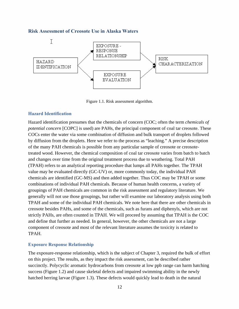
Risk Assessment of Creosote Use in Alaska Waters

Figure 1.1. Risk assessment algorithm.

Hazard Identification

Hazard identification presumes that the chemicals of concern (COC; often the term chemicals of potential concern [COPC] is used) are PAHs, the principal component of coal tar creosote. These COCs enter the water via some combination of diffusion and bulk transport of droplets followed by diffusion from the droplets. Here we refer to the process as “leaching.” A precise description of the many PAH chemicals is possible from any particular sample of creosote or creosote-treated wood. However, the chemical composition of coal tar creosote varies from batch to batch and changes over time from the original treatment process due to weathering. Total PAH (TPAH) refers to an analytical reporting procedure that lumps all PAHs together. The TPAH value may be evaluated directly (GC-UV) or, more commonly today, the individual PAH chemicals are identified (GC-MS) and then added together. Thus COC may be TPAH or some combinations of individual PAH chemicals. Because of human health concerns, a variety of groupings of PAH chemicals are common in the risk assessment and regulatory literature. We generally will not use those groupings, but rather will examine our laboratory analysis using both TPAH and some of the individual PAH chemicals. We note here that there are other chemicals in creosote besides PAHs, and some of the chemicals, such as furans and diphenyls, which are not strictly PAHs, are often counted in TPAH. We will proceed by assuming that TPAH is the COC and define that further as needed. In general, however, the other chemicals are not a large component of creosote and most of the relevant literature assumes the toxicity is related to TPAH.

Exposure Response Relationship

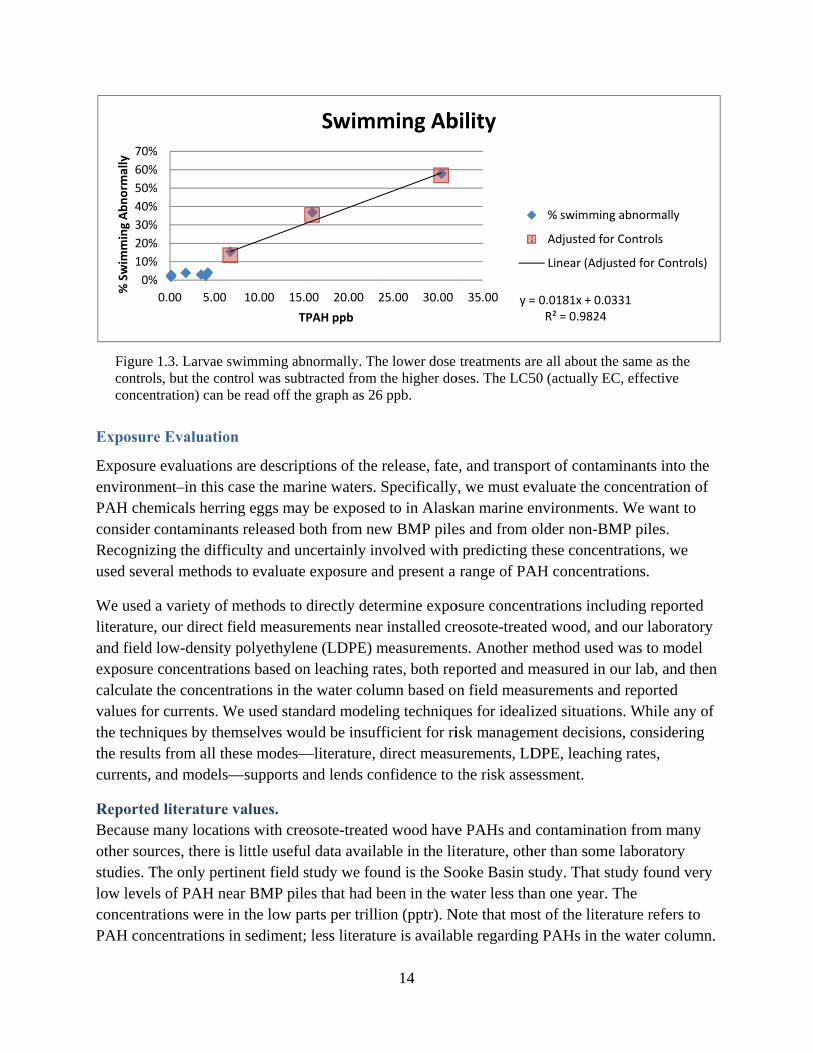
The exposure-response relationship, which is the subject of Chapter 3, required the bulk of effort on this project. The results, as they impact the risk assessment, can be described rather succinctly. Polycyclic aromatic hydrocarbons from creosote at low ppb range can harm hatching success (Figure 1.2) and cause skeletal defects and impaired swimming ability in the newly hatched herring larvae (Figure 1.3). These defects would quickly lead to death in the natural

13

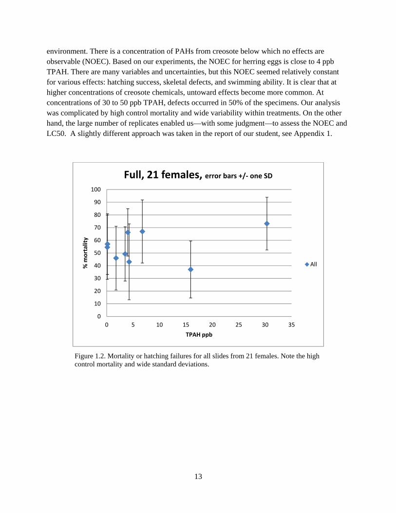
environment. There is a concentration of PAHs from creosote below which no effects are observable (NOEC). Based on our experiments, the NOEC for herring eggs is close to 4 ppb TPAH. There are many variables and uncertainties, but this NOEC seemed relatively constant for various effects: hatching success, skeletal defects, and swimming ability. It is clear that at higher concentrations of creosote chemicals, untoward effects become more common. At concentrations of 30 to 50 ppb TPAH, defects occurred in 50% of the specimens. Our analysis was complicated by high control mortality and wide variability within treatments. On the other hand, the large number of replicates enabled us—with some judgment—to assess the NOEC and LC50. A slightly different approach was taken in the report of our student, see Appendix 1.

Figure 1.2. Mortality or hatching failures for all slides from 21 females. Note the high control mortality and wide standard deviations.

0

10

20

30

40

50

60

70

80

90

100

0 5 10 15 20 25 30 35

% m

ortality

TPAH ppb

Full, 21 females, error bars +/‐ one SD

All

Figurecontroconcen

Exposur

ExposureenvironmPAH checonsider Recognizused seve

We used literatureand fieldexposurecalculatevalues fothe technthe resultcurrents,

ReportedBecause other soustudies. Tlow levelconcentraPAH con

0%

10%

20%

30%

40%

50%

60%

70%

% Swim

ming Abnorm

ally

e 1.3. Larvae sls, but the conntration) can b

re Evaluatio

e evaluationsment–in this emicals herricontaminan

zing the diffieral methods

a variety of e, our direct fd low-densitye concentrati the concent

or currents. Wniques by thets from all thand models

d literaturemany locati

urces, there iThe only perls of PAH neations were

ncentrations

%

%

%

%

%

%

%

%

0.00 5.00

swimming abntrol was subbe read off th

on

s are descripcase the maring eggs mayts released b

ficulty and uns to evaluate

f methods to field measury polyethylenons based ontrations in thWe used stanemselves wohese modes——supports a

values. ons with creis little usefurtinent field sear BMP pilin the low pain sediment;

10.00 15.

T

bnormally. Thbtracted from he graph as 26

ptions of the rine waters.y be exposedboth from nencertainly ine exposure an

directly deterements nearne (LDPE) mn leaching ra

he water colundard modeliould be insuf—literature, dand lends co

eosote-treateul data availastudy we foues that had barts per trilli; less literatu

.00 20.00 2

TPAH ppb

Swimm

14

he lower dose the higher do

6 ppb.

release, fateSpecificallyd to in Alaskew BMP pilenvolved withnd present a

ermine expor installed crmeasuremenates, both repumn based oing techniqufficient for ridirect measu

onfidence to

d wood haveable in the litund is the Sobeen in the wion (pptr). Nure is availab

25.00 30.00

ming Ab

treatments aroses. The LC5

e, and transpy, we must evkan marine ees and from oh predicting t

range of PA

osure concenreosote-treatnts. Another mported and mn field meas

ues for idealiisk managemurements, LDthe risk asse

e PAHs and terature, othooke Basin swater less thaNote that mosble regarding

y =35.00

bility

re all about th50 (actually E

ort of contamvaluate the cenvironmentolder non-Bthese concen

AH concentra

ntrations incled wood, anmethod used

measured in surements anized situation

ment decisionDPE, leachinessment.

contaminatiher than somstudy. That san one year. st of the literg PAHs in th

= 0.0181x + 0.0R² = 0.9824

% swimmin

Adjusted fo

Linear (Adju

he same as theEC, effective

minants intoconcentrations. We want tMP piles. ntrations, weations.

luding reportnd our laborad was to modour lab, and

nd reported ns. While anns, considering rates,

ion from mae laboratorystudy found v

The rature refers he water colu

0331

g abnormally

or Controls

usted for Contr

e

o the n of to

e

ted atory del

d then

ny of ing

any y very

to umn.

rols)

15

Our direct field measurements. We took nine water samples near installed creosote-treated wood in harbors near Juneau, Alaska. The wood had been in place for a long time: Otter Way/Indian Cove/NPS from 1966, Auke Bay Marine Science dock from before the late 1970s with additions in the mid-1980s, and Aurora Harbor from 1963. Most of the field measurements were quite low, averaging 314 pptr TPAH; however, two were higher, 5 and 8 ppb TPAH, but field records indicate these were anomalies.

LDPE measurements. Low-density polyethylene plastic has a high affinity for hydrocarbons and rapidly extracts them from the surrounding water. We put LDPE samplers in the treatment waters at our toxicity tests and thus have accurate representations of the mass of PAH in each sampler versus the average concentrations in the water. From these samplers we can compute Rs, the sampling rate, which converts mass in the sampler into concentrations in the water column. We have nine LDPE samples from water near the docks mentioned in the preceding paragraph.

Applying the Rs to our field samples at three Juneau-area harbors, we find that the typical TPAH ranges from 168 to 2910 pptr, with an average of 675 pptr TPAH. These field samples contain PAHs from sources other than the creosote from the piles; although, we note that the samplers close to the piles had higher concentrations than the samplers placed 1 meter or 10 meters away. [Work is currently in progress by NMFS to take more LDPE samples in the same region and further statistically analyze our samples.] The field samples were taken in locations with many piles, but the piles, which were certainly not BMP, had been in place for a long time.

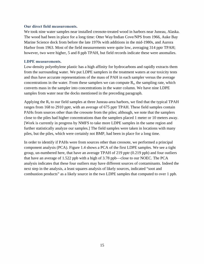
In order to identify if PAHs were from sources other than creosote, we performed a principal component analysis (PCA). Figure 1.4 shows a PCA of the first LDPE samples. We see a tight group, un-numbered here, that have an average TPAH of 219 pptr (0.219 ppb) and four outliers that have an average of 1.522 ppb with a high of 3.78 ppb—close to our NOEC. The PCA analysis indicates that these four outliers may have different sources of contaminants. Indeed the next step in the analysis, a least squares analysis of likely sources, indicated “soot and combustion products” as a likely source in the two LDPE samples that computed to over 1 ppb.

16

Figure 1.4. Principal component analysis of 9 LDPE samples. The sample numbers for the outliers are given; the numbers for the tight group were omitted for clarity.

Modeling. Source. For new creosote piles, there are models that predict the rate of leaching. These

models generally report loss of creosote as an entity, rather than the PAH chemicals in creosote. For new BMP piles, the minimum specified retention and actual retention are known. The actual retention varies somewhat and may be above the stated minimum retention when the pile is shipped from the treater. Some of the more-volatile components are lost during the shipping, processing, and storage.

A graph of leaching rate results is shown in Figure 1.5.

17

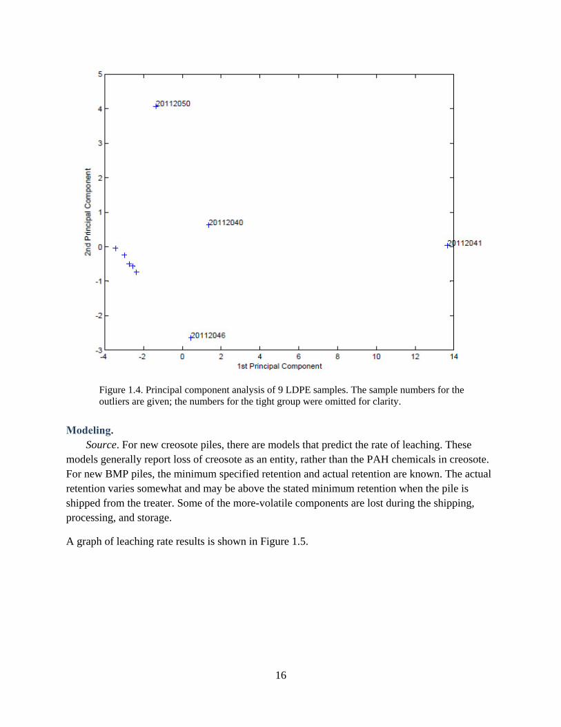
Figure 1.5. Leaching rates of treatments during the 15 day tox experiment and 15 days after. Regression equation refers to the average of Treatments IV, V, and VI. [Appendix Excel 4.2]

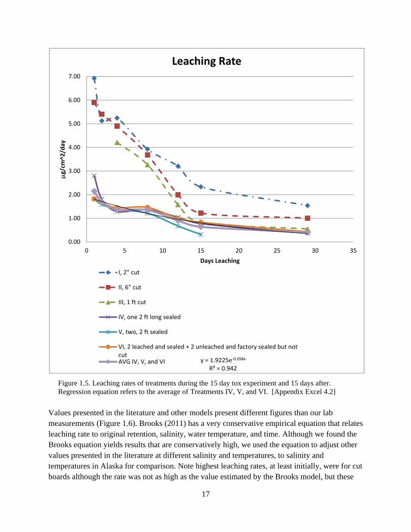
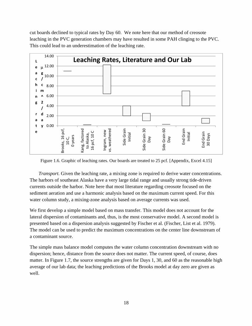
Values presented in the literature and other models present different figures than our lab measurements (Figure 1.6). Brooks (2011) has a very conservative empirical equation that relates leaching rate to original retention, salinity, water temperature, and time. Although we found the Brooks equation yields results that are conservatively high, we used the equation to adjust other values presented in the literature at different salinity and temperatures, to salinity and temperatures in Alaska for comparison. Note highest leaching rates, at least initially, were for cut boards although the rate was not as high as the value estimated by the Brooks model, but these

y = 1.9225e‐0.058x

R² = 0.942

0.00

1.00

2.00

3.00

4.00

5.00

6.00

7.00

0 5 10 15 20 25 30 35

g/cm^2/day

Days Leaching

Leaching Rate

I, 2" cut

II, 6" cut

III, 1 ft cut

IV, one 2 ft long sealed

V, two, 2 ft sealed

VI, 2 leached and sealed + 2 unleached and factory sealed but notcutAVG IV, V, and VI

18

cut boards declined to typical rates by Day 60. We note here that our method of creosote leaching in the PVC generation chambers may have resulted in some PAH clinging to the PVC. This could lead to an underestimation of the leaching rate.

Figure 1.6. Graphic of leaching rates. Our boards are treated to 25 pcf. [Appendix, Excel 4.15]

Transport. Given the leaching rate, a mixing zone is required to derive water concentrations. The harbors of southeast Alaska have a very large tidal range and usually strong tide-driven currents outside the harbor. Note here that most literature regarding creosote focused on the sediment aeration and use a harmonic analysis based on the maximum current speed. For this water column study, a mixing-zone analysis based on average currents was used.

We first develop a simple model based on mass transfer. This model does not account for the lateral dispersion of contaminants and, thus, is the most conservative model. A second model is presented based on a dispersion analysis suggested by Fischer et al. (Fischer, List et al. 1979). The model can be used to predict the maximum concentrations on the center line downstream of a contaminant source.

The simple mass balance model computes the water column concentration downstream with no dispersion; hence, distance from the source does not matter. The current speed, of course, does matter. In Figure 1.7, the source strengths are given for Days 1, 30, and 60 as the reasonable high average of our lab data; the leaching predictions of the Brooks model at day zero are given as well.

0.00

2.00

4.00

6.00

8.00

10.00

12.00

14.00

Brooks, 16 pcf,

10 C,

0 years

Kang, factored

to Alaska,

16 pcf, 10 C

Ingram

, new

vs. w

eathered

Side Grain

Initial

Side Grain 30

Day

Side Grain 60

Day

End Grain

Initial

End Grain

30 Days

L

e

a

c

h

i

n

g

r

a

t

e

g

/

c

m

^

2

/

d

a

y

Leaching Rates, Literature and Our Lab

19

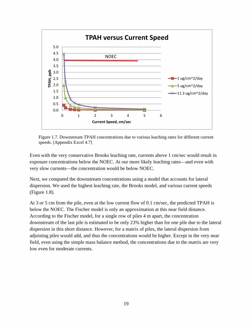
Figure 1.7. Downstream TPAH concentrations due to various leaching rates for different current speeds. [Appendix Excel 4.7]

Even with the very conservative Brooks leaching rate, currents above 1 cm/sec would result in exposure concentrations below the NOEC. At our more likely leaching rates—and even with very slow currents—the concentration would be below NOEC.

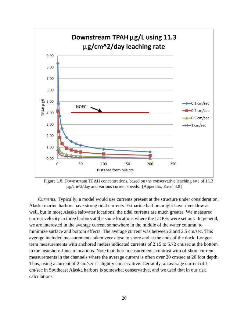
Next, we computed the downstream concentrations using a model that accounts for lateral dispersion. We used the highest leaching rate, the Brooks model, and various current speeds (Figure 1.8).

At 3 or 5 cm from the pile, even at the low current flow of 0.1 cm/sec, the predicted TPAH is below the NOEC. The Fischer model is only an approximation at this near field distance. According to the Fischer model, for a single row of piles 4 m apart, the concentration downstream of the last pile is estimated to be only 23% higher than for one pile due to the lateral dispersion in this short distance. However, for a matrix of piles, the lateral dispersion from adjoining piles would add, and thus the concentrations would be higher. Except in the very near field, even using the simple mass balance method, the concentrations due to the matrix are very low even for moderate currents.

0.0

0.5

1.0

1.5

2.0

2.5

3.0

3.5

4.0

4.5

5.0

0 1 2 3 4 5 6

TPAH, p

pb

Current Speed, cm/sec

TPAH versus Current Speed

1 ug/cm^2/day

5 ug/cm^2/day

11.3 ug/cm^2/day

NOEC

20

Figure 1.8. Downstream TPAH concentrations, based on the conservative leaching rate of 11.3

g/cm^2/day and various current speeds. [Appendix, Excel 4.8]

Currents. Typically, a model would use currents present at the structure under consideration. Alaska marine harbors have strong tidal currents. Estuarine harbors might have river flow as well, but in most Alaska saltwater locations, the tidal currents are much greater. We measured current velocity in three harbors at the same locations where the LDPEs were set out. In general, we are interested in the average current somewhere in the middle of the water column, to minimize surface and bottom effects. The average current was between 2 and 2.5 cm/sec. This average included measurements taken very close to shore and at the ends of the dock. Longer-term measurements with anchored meters indicated currents of 2.15 to 5.72 cm/sec at the bottom in the nearshore Juneau locations. Note that these measurements contrast with offshore current measurements in the channels where the average current is often over 20 cm/sec at 20 foot depth. Thus, using a current of 2 cm/sec is slightly conservative. Certainly, an average current of 1 cm/sec in Southeast Alaska harbors is somewhat conservative, and we used that in our risk calculations.

0.00

1.00

2.00

3.00

4.00

5.00

6.00

7.00

8.00

9.00

0 50 100 150 200 250

TPAH g/l

Distance from pile cm

Downstream TPAH g/L using 11.3 g/cm^2/day leaching rate

0.1 cm/sec

0.2 cm/sec

0.5 cm/sec

1 cm/sec

NOEC

21

ACZA We determined that ACZA should not be used for submerged glulams – it is not listed for this application by the AWPA or the CSA (AWPA 2010, Canadian Standards Association 2012). We identified poor performance of ACZA piles in one location, and anecdotal evidence from designers, constructors, and suppliers of treated wood suggest ACZA-treated piles and sawn lumber, used submerged or in the splash zone, would not have the service life of creosote-treated lumber. However for the short term, it is clear that ACZA is comparable to creosote, but we lack long term comparative testing. We were not able to determine that wood treatment with ACZA would be less toxic to herring eggs than treatment with creosote. The toxicity and risk evaluation of both preservatives in the water column is quite similar despite their very different chemistry.

Risk Characterization

Risk characterization is a statement of the likelihood of harm, based on exposure concentrations and the dose-response relationship. Since both the exposure concentrations and the dose-response relationship have uncertainty associated with them, the risk characterization must evaluate and express these uncertainties.

The recommendations and caveats for creosote in our earlier report were based on sediment toxicity, and they can be applied directly to water column toxicity of creosote to herring eggs. Unless the waters are stagnant or polluted, or the sediments are anaerobic, use of creosote in submerged timbers is unlikely to harm herring eggs in the vicinity of piles. Although ACZA was not the prime focus of our lab research, the literature indicates that those same recommendations and caveats apply to ACZA.

If the assumption of the overall project is that the area directly beneath and alongside the structure will be lost as fish habitat, then the recommendations above are sufficient. If the area beneath the structure is important fish habitat, for example, if herring are likely to spawn on the piles and submerged structures, then more research and analysis is required. Because our calculations are not dispositive in the very near field, there may be high concentrations of PAH within a few inches to a foot or two of the structures. Our leaching studies indicate that the rate is very low after 60 days. At Day 60, the mass balance model indicates 120 pptr even for 0.1 cm/sec currents, 33-fold less than the NOEC. However, the concentrations may be higher directly in lee of the pile and close to it.

For the case where biologists know that herring will spawn directly on newly installed piles, we expect that this will result in high mortality of the eggs. This level of mortality may be due to PAH migration from the pile to the lipophilic egg, but also may be due to toxicity of the microlayer of bacteria on the pile, since both treated and untreated wood quickly—within weeks—become “slimy” with microfouling. Literature did not indicate any reason to believe that ACZA would be superior to creosote in that regard. Even though copper is toxic to many marine invertebrates, marine bacteria quickly colonize ACZA wood as well as creosote. Bacteria that

22

utilize hydrocarbons abound in the marine environment. We suspect that these are chief inhabitants of the slime layer of creosote-treated wood. Macrofouling, barnacles, and seaweed, which would serve to discourage herring spawning or hold the eggs away from the wood, usually are prominent after a few months.

Although we have not been able to test our finding precisely, it is our recommendation that if herring stocks are stressed, installation of newly treated wood should be delayed until after the spawning season, or completed at least 60 days before the start of spawning. It seems probable that as leaching rates decrease and macrofouling becomes prominent, harm to the eggs becomes less likely. For example, using the conservative simple mass balance model, at the 60 day leaching rate and with a desire LC10—which is approximately 8.2 ppb TPAH—a current of only 0.0014 cm/sec would result in lower concentrations. It seems likely that even in the lee of a pile in a moderate current an egg would need to be very close to the pile, in some type of boundary layer, to experience currents slower than that.

Uncertainties

We are confident about the recommendations we have given; however, we now want to mention the uncertainties in our analysis:

The egg-hatching success studies were characterized by high control mortality and large variation, which limits some of the inferential statistics. The large number of replicates—21 for each of two controls and seven treatments—allows some confidence in the designation of NOEC at 4 ppb—which is in general agreement, but slightly lower than, the NOEC of herring eggs exposed to petroleum-derived TPAH. Regarding LC50, our confidence range is much wider.

Our leaching measurements are somewhat different from the findings of other studies but still within the same range of values—which is not surprising since others used different testing conditions and species of wood. Because the number of our experiments gave us a good opportunity to measure how much PAH was released, we have some confidence in our leaching numbers. We note that the use of PVC in the generation chambers creates some uncertainty in our leaching analysis.

The models are limited. The simple mass balance calculation is overly conservative, and the model based on Fischer is not definitive in the near field.

The currents were below the recommended lower speeds for the equipment we used. However, the operator, who has extensive experience with current meters, feels that the measurements are accurate, and they comport with the published data we have on currents.

We have confidence in the mass of TPAHs in our LDPE samplers and its ability to accurately capture concentrations found in the laboratory test water. Conversion to concentrations of water found in the field is not an exact science, but our computed concentrations are close to those measured directly in the field water and our conversion factor matches several from the

23

literature. Thus, we have confidence in our estimate of TPAH concentrations found in the field based on the LDPE. Confidence in our least squares analysis to determine the source of PAH is weakened by the lack of PAH profiles from water columns contaminated from one source. Our use of sediment PAH profiles requires an untested assumption – that PAH in the water above is in the same proportion as PAH in the sediment. On the other hand, the PCA analysis of the water samples is a well-established technique and clearly points to other sources of contamination for the samples with high TPAH. Thus, we have confidence that the high samples are anomalies, but less confidence in their sources.

Our review of ACZA toxicity and its comparison to creosote suffers from a lack of data on marine water column toxicity to herring eggs. Based on extrapolation from data on a similar copper-based preservative, CCA, we conclude that there is little difference between the toxicity of ACZA and the toxicity of creosote in the water column at levels likely to leach from treated marine wood. We have confidence in this conclusion based on our own work, the work of Dr. Brooks for the WWPI and Environment Canada, and the EPA RED regarding creosote and the various EPA RED documents for the ACZA components. Most recent EPA actions regarding the CCA relate to human health effects of chromated arsenates, not their toxicity in the marine environment.

24

Chapter 2. Creosote: Hazard Identification and Chemistry of Creosote and ACZA

Introduction

Our earlier report identified PAHs from creosote transported into the sediment as the COC. That report noted that PAHs from creosote in the water column were generally not of great concern to pelagic species, since the lighter PAHs quickly evaporate or are biodegraded and heavier PAHs are transported into the sediment. The report also noted that PAHs are ubiquitous in the marine environment, and most organisms have means of biotransforming and eliminating them. The report agreed with the EPA, WWPI, and NMFS that a risk assessment was needed if the proposed construction involved very large quantities of creosoted wood or if the sediments were anaerobic or already polluted. The resultant risk assessment would then be used to inform risk management decisions that would consider fish habitats, threatened or endanger species, the economic impacts, public safety, and benefits to society if the project was to proceed. The risk management decision would evaluate the costs and benefits of the options, while recognizing that not all of the costs or benefits can be expressed in dollars.

Earlier Recommendations

A major new project in the marine environment will consume some of the fish habitat and impact use of the project site and perhaps nearby waters. For a pier, the region under the pier and the nearby water churned by propellers would be lost as habitat. For such a project, the choice of wood preservative will likely have no effect on the disturbed region. For smaller projects and ancillary structures, the disturbance is likely to be small and the choice of wood preservative may have some local significance. Although most of the earlier literature reported on the risks due to creosote-derived PAHs in the sediment, we recognized that some literature implied a very high mortality in herring eggs spawned directly onto creosote-treated piles. Since herring stocks are stressed in some parts of Southeast Alaska, we suggested further research into the toxicity of creosote-derived PAHs on or near marine piles, and that topic is the chief object of this research. We combined this information with information about ACZA, the other wood preservative used in marine environments in Alaska, to help make a decision about wood preservation.

Hazard Identification for Creosote

To determine environmental risk from creosote, we start by identifying chemicals in creosote that are likely to be of concern. While PAHs are the chemical compounds in creosote most often named, creosote also contains many other chemicals including phenols and heterocycles (see Appendix 2.1 for a breakdown of other chemicals). In our analysis, we note that few researchers include some of these chemicals in their analysis; most researchers do not. We note that most of these non-PAH chemicals are only in small proportion. Therefore, other than noting their existence here, we will assume they are not substantial contributors to toxicity.

Regarding PAH analytes, there is a long list of potential PAH chemicals. Some researchers ignore less-common PAHs; other researchers combine them in logical groupings. When we used

25

data sets that have a slightly different list of PAHs, we adjusted the data as best we could. Most of these adjustments are for minor contributors. Bi-phenyl is often included as a PAH, although technically it is not. A much more important distinction is between parent PAH and the alkylated congeners. These congeners may have profound effects on the toxicity, and they certainly change the physical chemistry, such as water solubility. These alkyl groups are often excluded from standards lists, such as the EPA “dirty 16 PAH” and other compilations. The summation of all the PAH analytes is referred to as total PAHs (TPAH) and includes all the analytes. We used 48 compounds for our analysis. Many of these compounds are in minute quantities in water. In Appendix 2.2, we present a list of creosote PAH chemicals in various listings of creosote and our analysis, and some standard abbreviations that we use in some of the charts and spreadsheets. We analyzed all the PAH compounds using GC-MS at NOAA NMFS Ted Stevens Marine Research Institute.

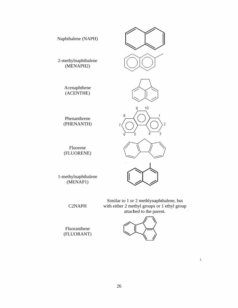
Especially in the early stages of testing, naphthalene and the alkylated naphthalenes make up almost half of the PAHs. In the later stages of testing, acenaphthene, phenanthrene, fluorene, and fluoranthene are significant, making up 60% of the PAH. Acenaphthene becomes the predominant PAH in later exposures. Figure 2.1 shows diagrams of the chemical structure of common PAHs.

Figure

Naph

2-me(M

A(A

P(P

(F

1-me

F(F

2.1 Diagrams

hthalene (NA

ethylnaphthaMENAPH2)

AcenaphtheneACENTHE)

PhenanthrenePHENANTH

Fluorene FLUORENE

ethylnaphtha(MENAP1)

C2NAPH

FluorantheneFLUORANT

s of the struct

APH)

alene )

e )

e H)

E)

alene

Simwith

e T)

ture of some c

26

milar to 1 orh either 2 me

attach

common PAH

r 2 methlynaethyl groups hed to the pa

H chemicals (

aphthalene, bor 1 ethyl gr

arent.

(sketches from

but roup

m Wikipedia)).

27

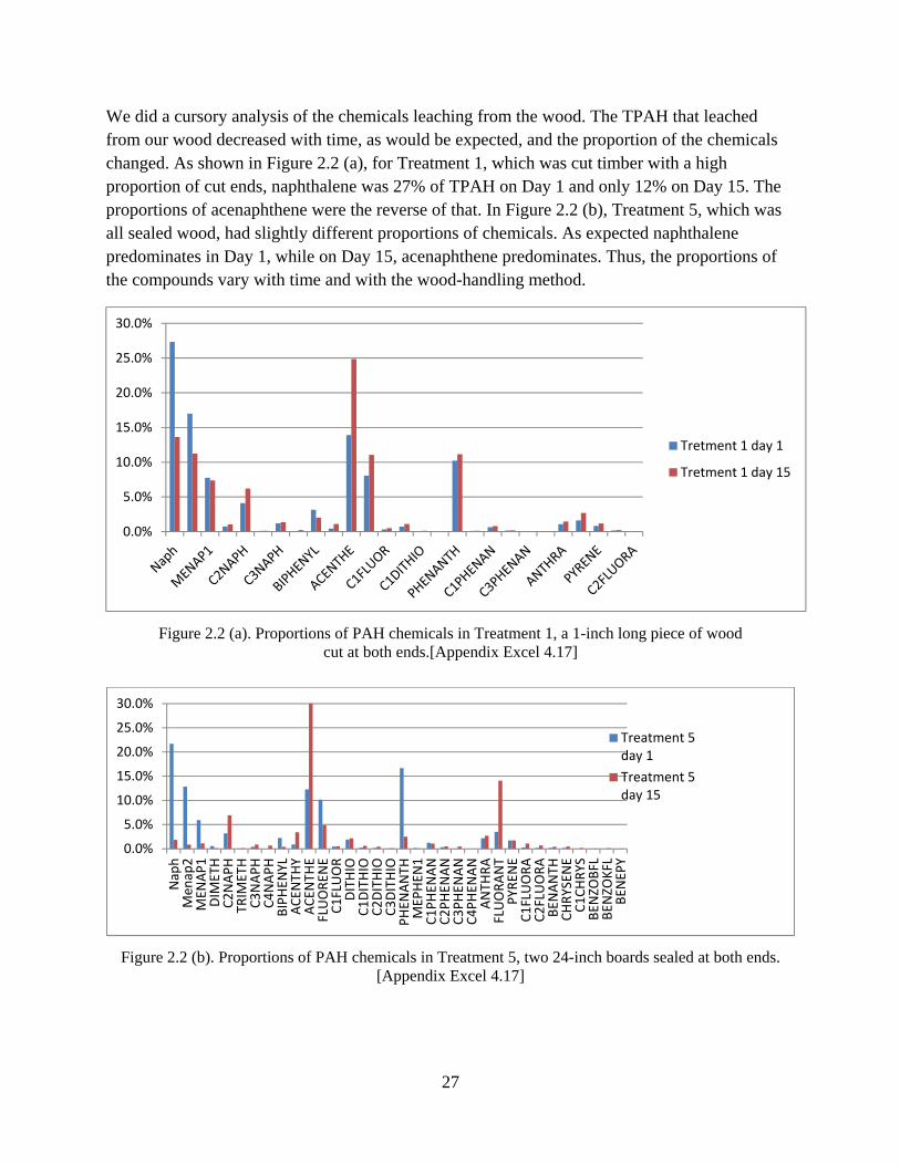
We did a cursory analysis of the chemicals leaching from the wood. The TPAH that leached from our wood decreased with time, as would be expected, and the proportion of the chemicals changed. As shown in Figure 2.2 (a), for Treatment 1, which was cut timber with a high proportion of cut ends, naphthalene was 27% of TPAH on Day 1 and only 12% on Day 15. The proportions of acenaphthene were the reverse of that. In Figure 2.2 (b), Treatment 5, which was all sealed wood, had slightly different proportions of chemicals. As expected naphthalene predominates in Day 1, while on Day 15, acenaphthene predominates. Thus, the proportions of the compounds vary with time and with the wood-handling method.

Figure 2.2 (a). Proportions of PAH chemicals in Treatment 1, a 1-inch long piece of wood cut at both ends.[Appendix Excel 4.17]

Figure 2.2 (b). Proportions of PAH chemicals in Treatment 5, two 24-inch boards sealed at both ends. [Appendix Excel 4.17]

0.0%

5.0%

10.0%

15.0%

20.0%

25.0%

30.0%

Tretment 1 day 1

Tretment 1 day 15

0.0%

5.0%

10.0%

15.0%

20.0%

25.0%

30.0%

Naph

Men

ap2

MEN

AP1

DIM

ETH

C2NAPH

TRIM

ETH

C3NAPH

C4NAPH

BIPHEN

YLACEN

THY

ACEN

THE

FLUOREN

EC1FLUOR

DITHIO

C1DITHIO

C2DITHIO

C3DITHIO

PHEN

ANTH

MEPHEN

1C1PHEN

AN

C2PHEN

AN

C3PHEN

AN

C4PHEN

AN

ANTH

RA

FLUORANT

PYR

ENE

C1FLUORA

C2FLUORA

BEN

ANTH

CHRYSEN

EC1CHRYS

BEN

ZOBFL

BEN

ZOKFL

BEN

EPY

Treatment 5day 1

Treatment 5day 15

28

Determining TPAH is the practical method of computing toxicity, but it should be kept in mind some compounds may be more toxic than others although this cannot be tested in environmentally relevant tests by isolating chemicals.

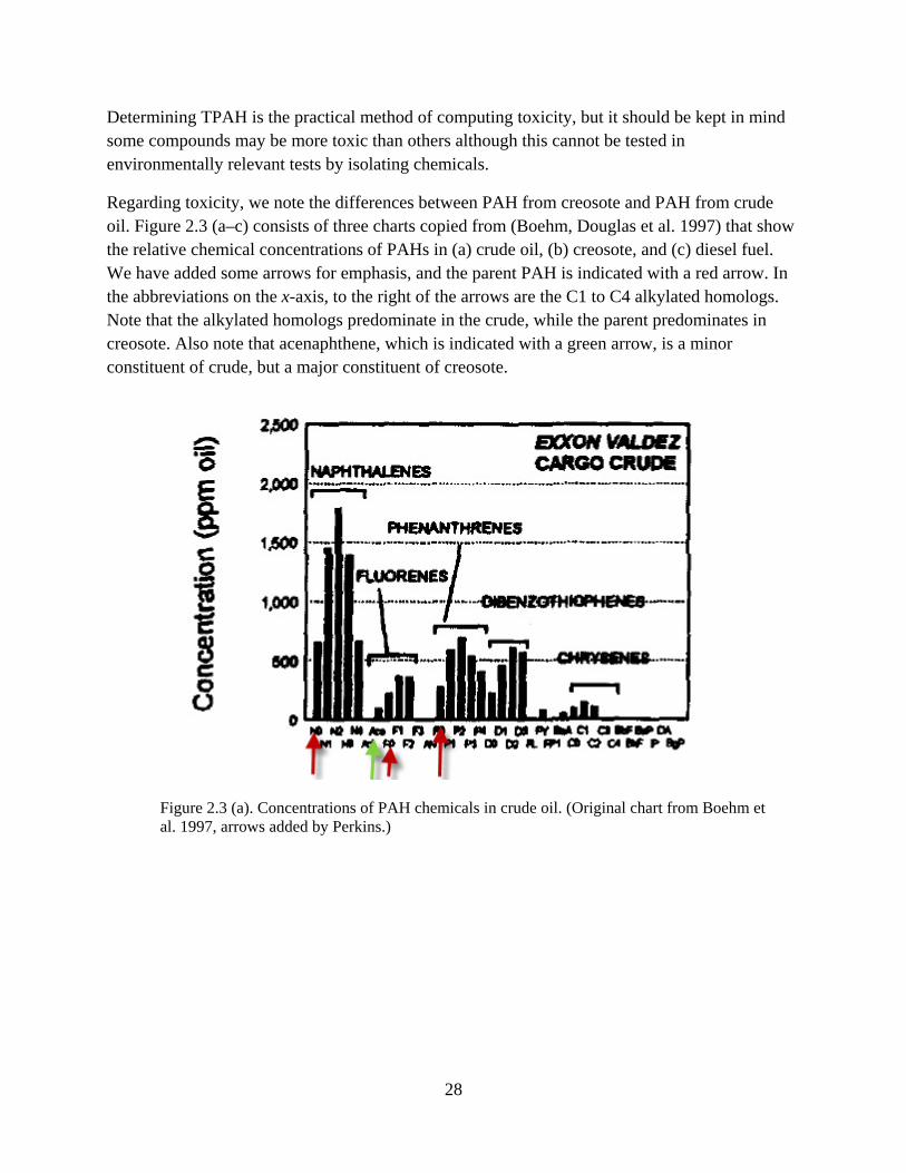
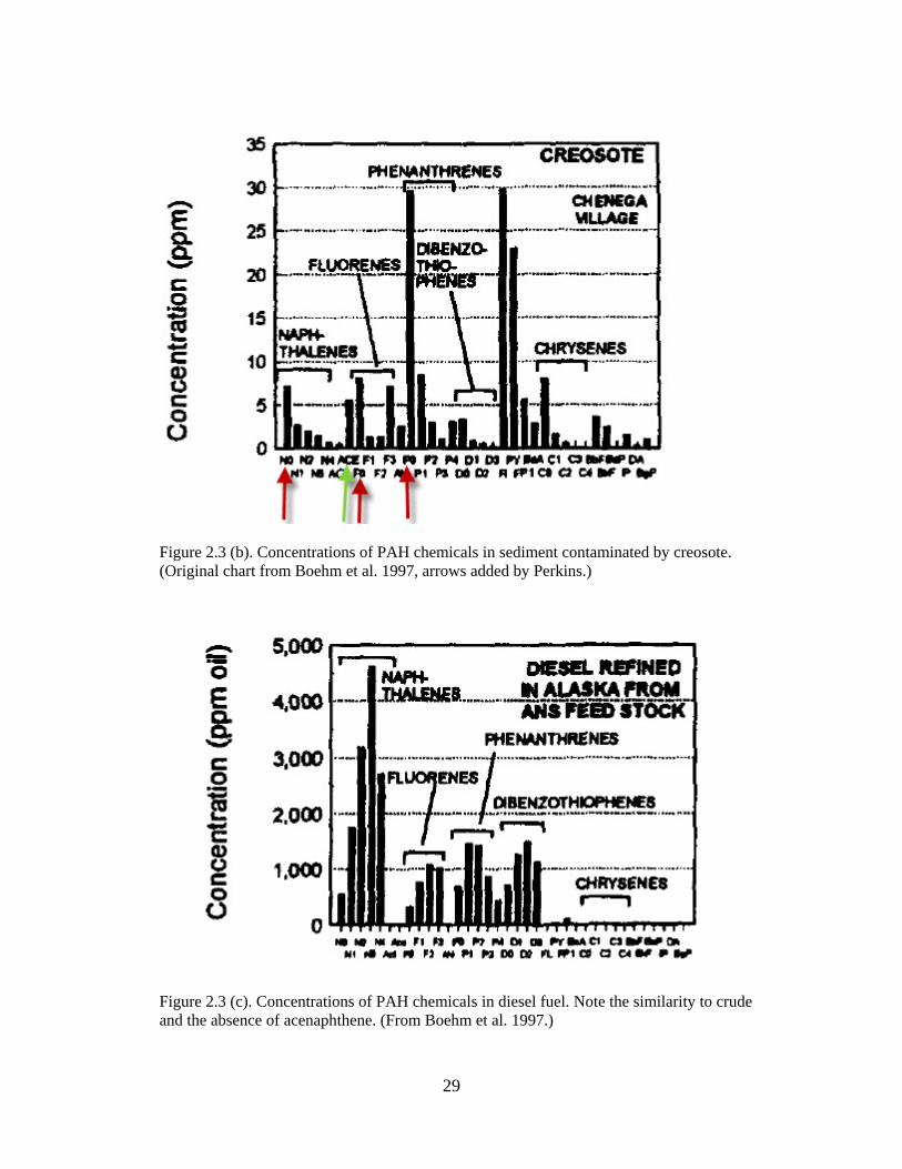
Regarding toxicity, we note the differences between PAH from creosote and PAH from crude oil. Figure 2.3 (a–c) consists of three charts copied from (Boehm, Douglas et al. 1997) that show the relative chemical concentrations of PAHs in (a) crude oil, (b) creosote, and (c) diesel fuel. We have added some arrows for emphasis, and the parent PAH is indicated with a red arrow. In the abbreviations on the x-axis, to the right of the arrows are the C1 to C4 alkylated homologs. Note that the alkylated homologs predominate in the crude, while the parent predominates in creosote. Also note that acenaphthene, which is indicated with a green arrow, is a minor constituent of crude, but a major constituent of creosote.

Figure 2.3 (a). Concentrations of PAH chemicals in crude oil. (Original chart from Boehm et al. 1997, arrows added by Perkins.)

29

Figure 2.3 (b). Concentrations of PAH chemicals in sediment contaminated by creosote. (Original chart from Boehm et al. 1997, arrows added by Perkins.)

Figure 2.3 (c). Concentrations of PAH chemicals in diesel fuel. Note the similarity to crude and the absence of acenaphthene. (From Boehm et al. 1997.)

30

Some evidence indicates that the toxicity of PAHs increases with the degree of alkylation. This seems likely for several reasons, but may be difficult to assess. The lipophilicity, measured as log Kow, increases with each alkyl group, and water solubility decreases. Thus, the more-alkylated compounds leach into the water slower than the less-alkylated compounds. In general, PAHs must become activated by oxygenating enzymes in the organism before their toxic potency is realized. Higher organisms have these enzymes, but it is assumed that eggs do not. Thus, for toxicity to eggs, some other mechanism of toxicity that does not depend on oxygenating enzymes is assumed. We must proceed using TPAH as our substance of concern but consider this information when comparing our toxicity data with the data of others.

Appendix 2.3 presents a list of PAH chemicals in creosote-treated wood, extracted from core samples.

For new piles there are models that predict the rate of creosote loss. These models generally relate to creosote as an entity, rather than specific PAH chemicals. For new BMP piles, the minimum specified retention is known. The actual retention varies somewhat and may be above the minimum retention when the pile is shipped from the treater. Some of the more volatile components are lost during the shipping process and storage.

ACZA Chemistry

A common trade name for ammoniacal copper zinc arsenate (ACZA) is Chemonite ®. ACZA is one member of a class of water-borne arsenical preservatives. ACZA is required for hard-to-treat western softwood, like Douglas-fir, the most common wood species in Alaska. Although water-borne, once in wood, the metal fixes to the wood and becomes insoluble. Note that copper and zinc leach from the ACZA-treated lumber in the marine environment. A more-common member of that class is CCA, chromated copper arsenate, for which many studies have been done. Arsenate is generally not considered an environmental hazard, but human health concerns related to direct human contact have led to agencies to recommend against CCA use in home consumer products. Due to an abundance of information on CCA and because copper—the most likely environmental contaminant—is common to both CCA and ACZA, we used some of the CCA data in our analysis. More on this topic is discussed in the chapter on ACZA.

Characteristics

Oil-type preservatives such as creosote do not fix within the wood, but form a coating on the cell walls. Creosote is an oil-borne preservative that resists leaching by the viscosity and insolubility of its component chemicals. Thus, creosote chemicals can and do leach for the life of the wood, but at a decreasing rate. Preservatives such an CCA (and presumably ACZA) fix in the wood through complex chemical reactions in which copper, arsenic, and chromium (and presumably zinc) form a soluble and insoluble complex with the lignocellulose components of the wood structure. The fixation of ACZA involves diffusion of ammonia out of the wood, which results in the precipitation of zinc arsenate, a leach-resistant compound (Morrell, Brooks et al. 2011)

31

Brooks (Brooks 2011) models the leaching of ACZA chemicals, with arsenic and zinc leaching

steady rates of 0.54 and 5.75 g/cm^2/day of arsenic and zinc, respectively, but notes a decline

in copper leaching with time, from 18.7 g/cm^2/day on Day 1 to 6.8 at the end of the year, holding that rate thereafter. Based on the Brooks Model and our calculations in Appendix 2.4, we note that those rates are similar to the leaching rate of TPAH from creosote (see Chapter 4).

32

Chapter 3. Dose Response

This chapter presents an overview and summary of the results, with some details about the calculation of the results. Appendix 1.1 is a full report on the testing procedures, with many details and photos.

General Introduction

An environmental risk assessment evaluates the likely response or effect of a contaminant of concern on a selected receptor. Since the effect is related to a dose or concentration, the risk assessor must determine the exposure dose the receptor is expected to receive. This exposure dose is usually varied over a range, and the effects are estimated for various doses. In ecological risk assessment, target receptors are selected that are presumably representative of the ecosystem under consideration, and ideally are sensitive receptors. Since the response of most receptors to most contaminants is unknown, laboratory testing, known simply as “tox testing,” is required to determine the likely response. However, as a practical matter, most tox testing is done with standard test species, to which typical responses to contaminants are known. Thus, both laboratory procedures and preliminary analysis of the results are standardized (Chapman 1995).

Unfortunately, environmental agencies do not have standard procedures for a risk assessment to determine the risk to herring eggs from creosote-preserved wood. Some scientific work has been reported and is discussed below. As a practical matter, we used procedures developed by others and reported in peer-reviewed scientific literature. However, since research projects differ in many respects, we often were guided by our judgment.

In reporting toxicity, two terms are important: “no observable effects concentration” (NOEC) and “lethal concentration to 50% of the subjects” (LC50). For risk management, NOEC is most important, since if concentrations are held below that level, damage to the receptors is unlikely. LC50 and other percentages are useful for estimating the amount of damage to populations if exposures are above the NOEC; it is also useful in comparing toxicity between different chemicals and classes of chemicals. (LC50 is properly written with the 50 in a subscript, but use of standard font is common.)

Overview of the Testing

Details of the testing, including photographs, are found in the Appendix. Herring were live-captured just before they were ready to spawn in late March and April 2011 and kept in tanks in NOAA labs until they were ready to release gametes in May. The herring were killed and gametes removed for ex situ fertilization. Eggs from 21 females were placed on slides, and the slides were placed in a sperm mixture. The slides were then placed in one of nine smaller aquaria tanks for exposure. Of the eggs from 21 females, 16 were placed in the open aquaria, and these were the intended primary subjects, while five were placed in screened bottles within the aquaria to test for fertilization success. The NOAA NMFS scientists who were helping us on the project had experience capturing, ripening, fertilizing, and the basic exposure scenario.

33

Water was supplied to the tanks from nine different supply cylinders: two controls, one water-only, one wood control, and seven different exposure regimes with various amounts of BMP creosote-treated wood. Samples of the water were taken and analyzed by GC/MS for 48 analytes, which were summed for TPAH. Eggs in the aquaria were observed for fertilization success, viability, and eyeing. At Day 15 of the 22-day cycle, slides with eggs from the group of 16 females were removed from the aquaria and placed into beakers with clean water and observed through hatching. We assessed hatching success, larval swimming ability, and the presence of skeletal deformities. The slides from the five females that were left in the aquaria were only assessed for hatching success.

Experimental Issues

Wood: Because PAHs must be leached from creosote-treated wood rather than added as a chemical, achieving accurate dosing was more complex than typical chemical or effluent tox testing. The original plan was to use only wood that had been pre-leached and end-sealed; however, the BMP wood of quantities that would fit into our experiment system did not leach sufficient PAHs for the range of concentrations needed. In order to overcome this, other combinations were used, including end cuts. Use of end cuts was not desirable, since the mix of PAHs would be at least slightly different than boards with the ends sealed. We performed detailed chemistry on the exposure water, and thus could observe the change in chemistry, which was slight. This is discussed later in this report. Exposure concentrations were not as evenly spaced as we would have liked, nor were the high end concentrations as high as we would have liked. None of this is unusual even in the standard tests of variable materials, such as wastewater effluent, but we mention it here for completeness.

Control mortality: Standard procedures call for no more than 10% mortality or effects in the controls. Of course, these standards generally apply to organisms that have been cultured for laboratory work. The same standards are indeed used for wild-captured organisms, but there is much greater tolerance for variability. For eggs there is no standard, but a review of published data indicate that mortalities are almost never less than 20% and some much higher. Much of this variability can be attributed to the eggs coming from different females and being fertilized by different males.

Egg loadings: Papers on egg testing using similar procedures suggest maximum egg loadings of 100 to 150 eggs per slide. Control mortality seems to improve with lower loadings, presumably due to less competition for oxygen. Our loadings averaged 135 eggs per slide with a standard deviation of 28 eggs per slide. Thus, most of our slides were within the criterion of 150 eggs per slide. Nonetheless, there was a weak correlation, r^2 = 0.56, between egg loadings and hatching success. Because the heavier loading was distributed at random, we had to choose whether to include all the slides or only those with less than 150 eggs or less than 100 eggs. However several doses had only one slide with less than 100 eggs. So, instead of 100, we increased the power of the analysis by using a threshold of 115 eggs per slide.

34

Issues Affecting Toxicity Evaluation

We were primarily interested in two numbers: the NOEC and the LC50, which are dependent variables. The independent variables were the doses/concentrations, expressed in TPAH.. Many standard procedures are available for extracting NOEC and EC50 from data, such as EPA (Chapman 1995) and many similar procedures. Our examination of the data regarding hatching success is slightly non-standard for several reasons.

1. We examined hatching success with a large numbers of eggs on glass slides. Also, control mortalities were higher than the 10% rule of thumb for typical environmental toxicity.

2. There were two controls—water only and water with untreated wood—thus we could use either of these, or an average of both. All three are reported.

3. The mortality in the controls was greater than the mortality in some of the low dose treatments.

4. For each dose, the variance of the data is large with an average CV of 43%.

5. The mortality did not increase regularly with dose. While some inversions are common, we have an unusual amount of them.

6. The standard for eggs on slides is 100 eggs per slide—many of our slides had more than 100 eggs on them. This standard is a rule of thumb that relates to eggs lumping together, decreasing the space between eggs and increasing competition for oxygen. If the eggs are separated and there is a strong and consistent flow of water, the number of eggs on a slide is not as important. Our laboratory researcher, Danielle Duncan, generally removed all the clumps and eggs near the edges, so there were no lumps of eggs in the study.

7. There was a weak correlation (R^2 = 0.56) between the number of eggs on a slide and the number of deaths in the control. Thus, we examined the data two ways: one method was to use the data from all slides and the other method was to examine the data only from slides that had 115 or fewer eggs and 150 or fewer eggs per slide.

The standard method of correcting for control deaths in data is called Abbott’s method. It is a straightforward method of correcting the proportions. Here, where pi is the proportion of mortalities in the i-th treatment and pc is the proportion in the control, Abbott’s method is just

)p( 1

)p( p

cci

If the pc is greater than the pi, which is not uncommon, the result is a negative percent. For some statistics, that point cannot be used. Thus, all pi with deaths greater than the

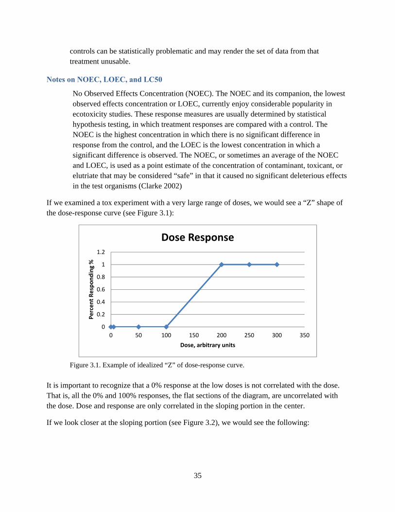
35

controls can be statistically problematic and may render the set of data from that treatment unusable.

Notes on NOEC, LOEC, and LC50

No Observed Effects Concentration (NOEC). The NOEC and its companion, the lowest observed effects concentration or LOEC, currently enjoy considerable popularity in ecotoxicity studies. These response measures are usually determined by statistical hypothesis testing, in which treatment responses are compared with a control. The NOEC is the highest concentration in which there is no significant difference in response from the control, and the LOEC is the lowest concentration in which a significant difference is observed. The NOEC, or sometimes an average of the NOEC and LOEC, is used as a point estimate of the concentration of contaminant, toxicant, or elutriate that may be considered “safe” in that it caused no significant deleterious effects in the test organisms (Clarke 2002)

If we examined a tox experiment with a very large range of doses, we would see a “Z” shape of the dose-response curve (see Figure 3.1):

Figure 3.1. Example of idealized “Z” of dose-response curve.

It is important to recognize that a 0% response at the low doses is not correlated with the dose. That is, all the 0% and 100% responses, the flat sections of the diagram, are uncorrelated with the dose. Dose and response are only correlated in the sloping portion in the center.

If we look closer at the sloping portion (see Figure 3.2), we would see the following:

0

0.2

0.4

0.6

0.8

1

1.2

0 50 100 150 200 250 300 350

Percent Responding %

Dose, arbitrary units

Dose Response

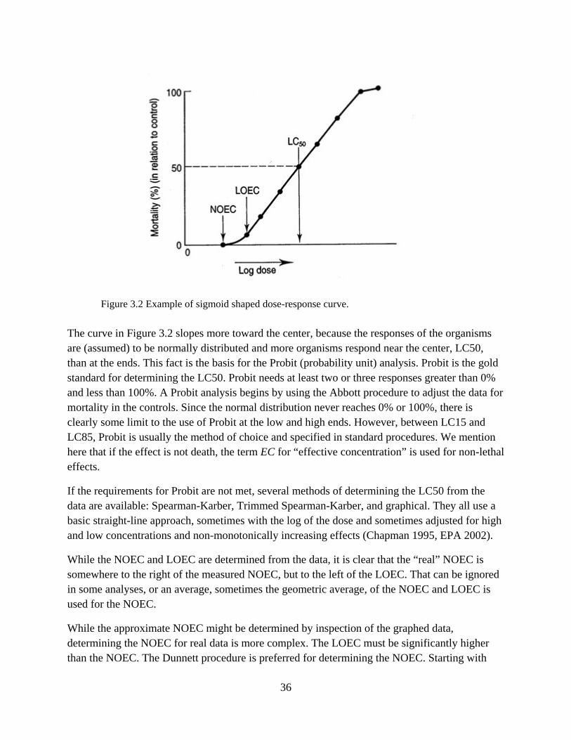
36

Figure 3.2 Example of sigmoid shaped dose-response curve.

The curve in Figure 3.2 slopes more toward the center, because the responses of the organisms are (assumed) to be normally distributed and more organisms respond near the center, LC50, than at the ends. This fact is the basis for the Probit (probability unit) analysis. Probit is the gold standard for determining the LC50. Probit needs at least two or three responses greater than 0% and less than 100%. A Probit analysis begins by using the Abbott procedure to adjust the data for mortality in the controls. Since the normal distribution never reaches 0% or 100%, there is clearly some limit to the use of Probit at the low and high ends. However, between LC15 and LC85, Probit is usually the method of choice and specified in standard procedures. We mention here that if the effect is not death, the term EC for “effective concentration” is used for non-lethal effects.

If the requirements for Probit are not met, several methods of determining the LC50 from the data are available: Spearman-Karber, Trimmed Spearman-Karber, and graphical. They all use a basic straight-line approach, sometimes with the log of the dose and sometimes adjusted for high and low concentrations and non-monotonically increasing effects (Chapman 1995, EPA 2002).

While the NOEC and LOEC are determined from the data, it is clear that the “real” NOEC is somewhere to the right of the measured NOEC, but to the left of the LOEC. That can be ignored in some analyses, or an average, sometimes the geometric average, of the NOEC and LOEC is used for the NOEC.

While the approximate NOEC might be determined by inspection of the graphed data, determining the NOEC for real data is more complex. The LOEC must be significantly higher than the NOEC. The Dunnett procedure is preferred for determining the NOEC. Starting with

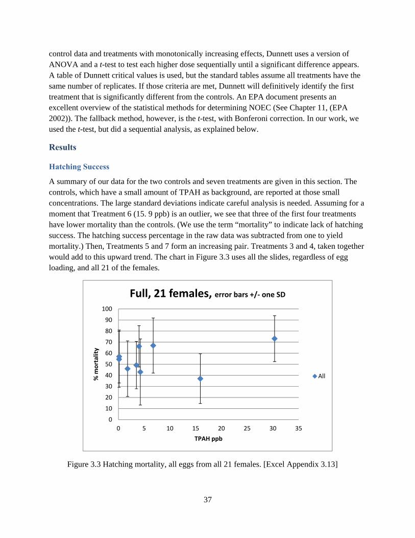
37

control data and treatments with monotonically increasing effects, Dunnett uses a version of ANOVA and a t-test to test each higher dose sequentially until a significant difference appears. A table of Dunnett critical values is used, but the standard tables assume all treatments have the same number of replicates. If those criteria are met, Dunnett will definitively identify the first treatment that is significantly different from the controls. An EPA document presents an excellent overview of the statistical methods for determining NOEC (See Chapter 11, (EPA 2002)). The fallback method, however, is the t-test, with Bonferoni correction. In our work, we used the t-test, but did a sequential analysis, as explained below.

Results

Hatching Success

A summary of our data for the two controls and seven treatments are given in this section. The controls, which have a small amount of TPAH as background, are reported at those small concentrations. The large standard deviations indicate careful analysis is needed. Assuming for a moment that Treatment 6 (15. 9 ppb) is an outlier, we see that three of the first four treatments have lower mortality than the controls. (We use the term “mortality” to indicate lack of hatching success. The hatching success percentage in the raw data was subtracted from one to yield mortality.) Then, Treatments 5 and 7 form an increasing pair. Treatments 3 and 4, taken together would add to this upward trend. The chart in Figure 3.3 uses all the slides, regardless of egg loading, and all 21 of the females.

Figure 3.3 Hatching mortality, all eggs from all 21 females. [Excel Appendix 3.13]

0

10

20

30

40

50

60

70

80

90

100

0 5 10 15 20 25 30 35

% m

ortality

TPAH ppb

Full, 21 females, error bars +/‐ one SD

All

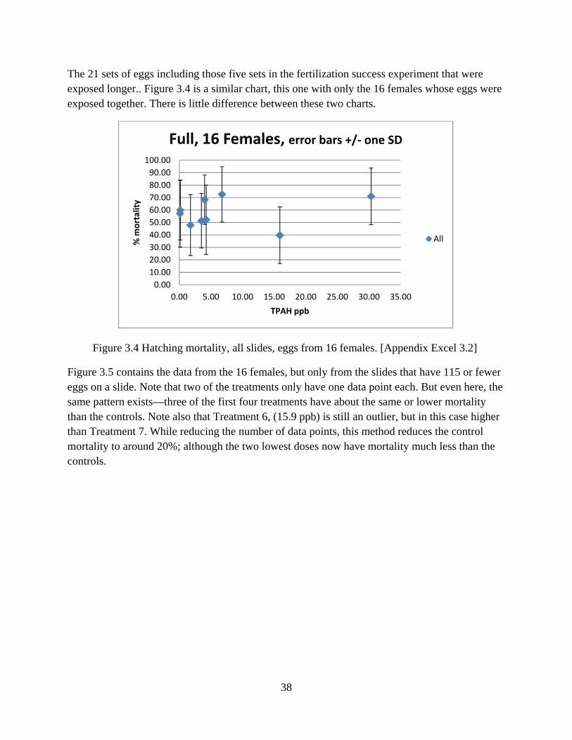
38

The 21 sets of eggs including those five sets in the fertilization success experiment that were exposed longer.. Figure 3.4 is a similar chart, this one with only the 16 females whose eggs were exposed together. There is little difference between these two charts.

Figure 3.4 Hatching mortality, all slides, eggs from 16 females. [Appendix Excel 3.2]

Figure 3.5 contains the data from the 16 females, but only from the slides that have 115 or fewer eggs on a slide. Note that two of the treatments only have one data point each. But even here, the same pattern exists—three of the first four treatments have about the same or lower mortality than the controls. Note also that Treatment 6, (15.9 ppb) is still an outlier, but in this case higher than Treatment 7. While reducing the number of data points, this method reduces the control mortality to around 20%; although the two lowest doses now have mortality much less than the controls.

0.00

10.00

20.00

30.00

40.00

50.00

60.00

70.00

80.00

90.00

100.00

0.00 5.00 10.00 15.00 20.00 25.00 30.00 35.00

% m

ortality

TPAH ppb

Full, 16 Females, error bars +/‐ one SD

All

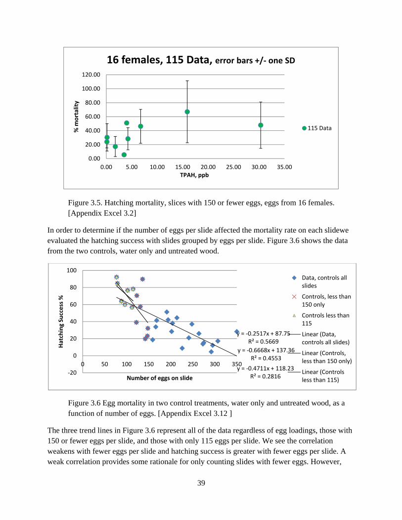
39

Figure 3.5. Hatching mortality, slices with 150 or fewer eggs, eggs from 16 females. [Appendix Excel 3.2]

In order to determine if the number of eggs per slide affected the mortality rate on each slidewe evaluated the hatching success with slides grouped by eggs per slide. Figure 3.6 shows the data from the two controls, water only and untreated wood.

Figure 3.6 Egg mortality in two control treatments, water only and untreated wood, as a function of number of eggs. [Appendix Excel 3.12 ]

The three trend lines in Figure 3.6 represent all of the data regardless of egg loadings, those with 150 or fewer eggs per slide, and those with only 115 eggs per slide. We see the correlation weakens with fewer eggs per slide and hatching success is greater with fewer eggs per slide. A weak correlation provides some rationale for only counting slides with fewer eggs. However,

0.00

20.00

40.00

60.00

80.00

100.00

120.00

0.00 5.00 10.00 15.00 20.00 25.00 30.00 35.00

% m

ortality 

TPAH, ppb

16 females, 115 Data, error bars +/‐ one SD

115 Data

y = ‐0.2517x + 87.75R² = 0.5669

y = ‐0.6668x + 137.36R² = 0.4553

y = ‐0.4711x + 118.23R² = 0.2816

‐20

0

20

40

60

80

100

0 50 100 150 200 250 300 350

Hatching Success %

Number of eggs on slide

Data, controls allslides

Controls, less than150 only

Controls less than115

Linear (Data,controls all slides)

Linear (Controls,less than 150 only)

Linear (Controlsless than 115)

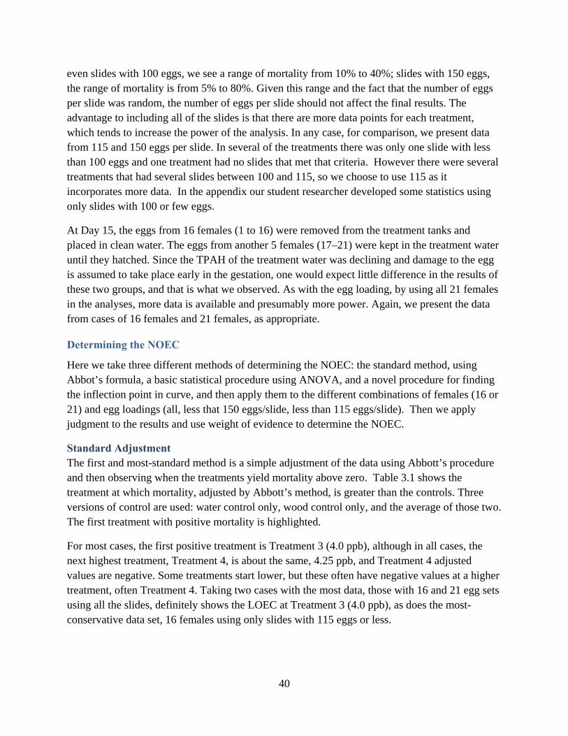
40

even slides with 100 eggs, we see a range of mortality from 10% to 40%; slides with 150 eggs, the range of mortality is from 5% to 80%. Given this range and the fact that the number of eggs per slide was random, the number of eggs per slide should not affect the final results. The advantage to including all of the slides is that there are more data points for each treatment, which tends to increase the power of the analysis. In any case, for comparison, we present data from 115 and 150 eggs per slide. In several of the treatments there was only one slide with less than 100 eggs and one treatment had no slides that met that criteria. However there were several treatments that had several slides between 100 and 115, so we choose to use 115 as it incorporates more data. In the appendix our student researcher developed some statistics using only slides with 100 or few eggs.

At Day 15, the eggs from 16 females (1 to 16) were removed from the treatment tanks and placed in clean water. The eggs from another 5 females (17–21) were kept in the treatment water until they hatched. Since the TPAH of the treatment water was declining and damage to the egg is assumed to take place early in the gestation, one would expect little difference in the results of these two groups, and that is what we observed. As with the egg loading, by using all 21 females in the analyses, more data is available and presumably more power. Again, we present the data from cases of 16 females and 21 females, as appropriate.

Determining the NOEC

Here we take three different methods of determining the NOEC: the standard method, using Abbot’s formula, a basic statistical procedure using ANOVA, and a novel procedure for finding the inflection point in curve, and then apply them to the different combinations of females (16 or 21) and egg loadings (all, less that 150 eggs/slide, less than 115 eggs/slide). Then we apply judgment to the results and use weight of evidence to determine the NOEC.

Standard Adjustment The first and most-standard method is a simple adjustment of the data using Abbott’s procedure and then observing when the treatments yield mortality above zero. Table 3.1 shows the treatment at which mortality, adjusted by Abbott’s method, is greater than the controls. Three versions of control are used: water control only, wood control only, and the average of those two. The first treatment with positive mortality is highlighted.

For most cases, the first positive treatment is Treatment 3 (4.0 ppb), although in all cases, the next highest treatment, Treatment 4, is about the same, 4.25 ppb, and Treatment 4 adjusted values are negative. Some treatments start lower, but these often have negative values at a higher treatment, often Treatment 4. Taking two cases with the most data, those with 16 and 21 egg sets using all the slides, definitely shows the LOEC at Treatment 3 (4.0 ppb), as does the most-conservative data set, 16 females using only slides with 115 eggs or less.

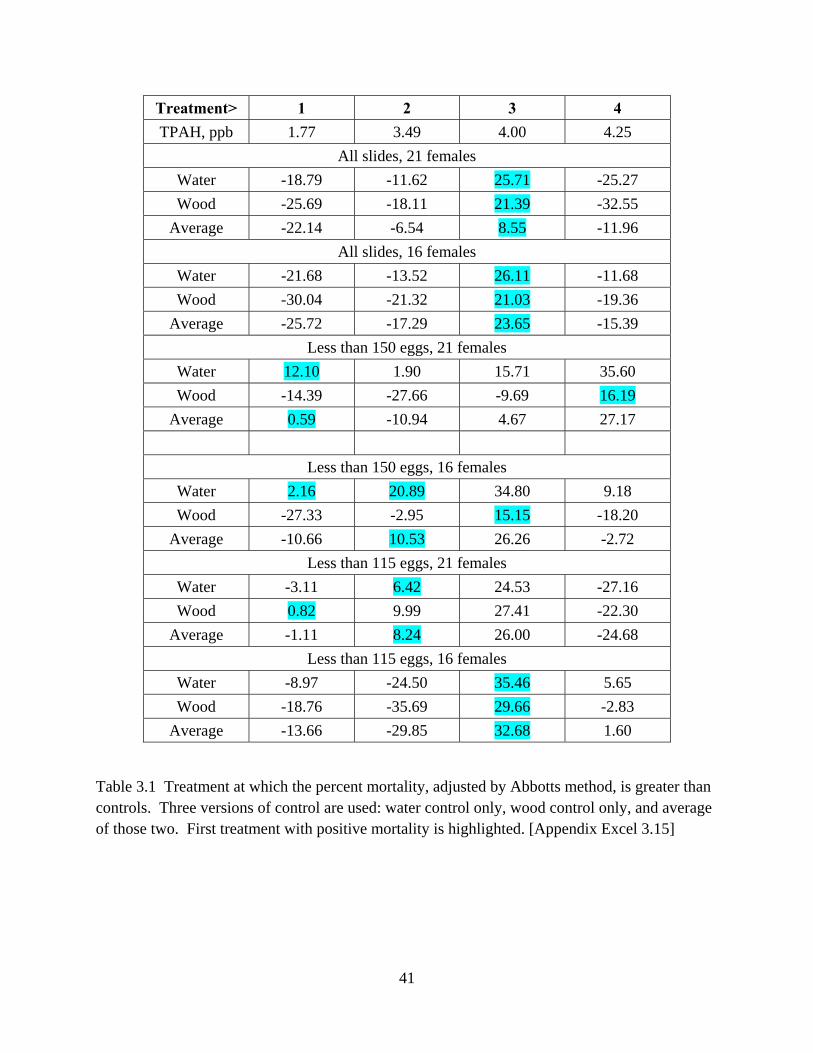
41

Treatment> 1 2 3 4

TPAH, ppb 1.77 3.49 4.00 4.25

All slides, 21 females

Water -18.79 -11.62 25.71 -25.27

Wood -25.69 -18.11 21.39 -32.55

Average -22.14 -6.54 8.55 -11.96

All slides, 16 females

Water -21.68 -13.52 26.11 -11.68

Wood -30.04 -21.32 21.03 -19.36

Average -25.72 -17.29 23.65 -15.39

Less than 150 eggs, 21 females

Water 12.10 1.90 15.71 35.60

Wood -14.39 -27.66 -9.69 16.19

Average 0.59 -10.94 4.67 27.17

Less than 150 eggs, 16 females

Water 2.16 20.89 34.80 9.18

Wood -27.33 -2.95 15.15 -18.20

Average -10.66 10.53 26.26 -2.72

Less than 115 eggs, 21 females

Water -3.11 6.42 24.53 -27.16

Wood 0.82 9.99 27.41 -22.30

Average -1.11 8.24 26.00 -24.68

Less than 115 eggs, 16 females

Water -8.97 -24.50 35.46 5.65

Wood -18.76 -35.69 29.66 -2.83

Average -13.66 -29.85 32.68 1.60

Table 3.1 Treatment at which the percent mortality, adjusted by Abbotts method, is greater than controls. Three versions of control are used: water control only, wood control only, and average of those two. First treatment with positive mortality is highlighted. [Appendix Excel 3.15]

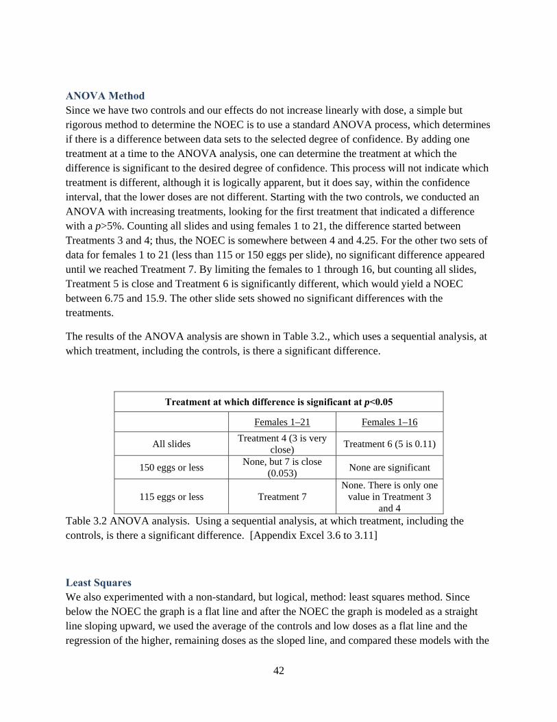
42

ANOVA Method Since we have two controls and our effects do not increase linearly with dose, a simple but rigorous method to determine the NOEC is to use a standard ANOVA process, which determines if there is a difference between data sets to the selected degree of confidence. By adding one treatment at a time to the ANOVA analysis, one can determine the treatment at which the difference is significant to the desired degree of confidence. This process will not indicate which treatment is different, although it is logically apparent, but it does say, within the confidence interval, that the lower doses are not different. Starting with the two controls, we conducted an ANOVA with increasing treatments, looking for the first treatment that indicated a difference with a p>5%. Counting all slides and using females 1 to 21, the difference started between Treatments 3 and 4; thus, the NOEC is somewhere between 4 and 4.25. For the other two sets of data for females 1 to 21 (less than 115 or 150 eggs per slide), no significant difference appeared until we reached Treatment 7. By limiting the females to 1 through 16, but counting all slides, Treatment 5 is close and Treatment 6 is significantly different, which would yield a NOEC between 6.75 and 15.9. The other slide sets showed no significant differences with the treatments.

The results of the ANOVA analysis are shown in Table 3.2., which uses a sequential analysis, at which treatment, including the controls, is there a significant difference.

Treatment at which difference is significant at p<0.05

Females 1–21 Females 1–16

All slides Treatment 4 (3 is very

close) Treatment 6 (5 is 0.11)

150 eggs or less None, but 7 is close

(0.053) None are significant

115 eggs or less Treatment 7 None. There is only one

value in Treatment 3 and 4

Table 3.2 ANOVA analysis. Using a sequential analysis, at which treatment, including the controls, is there a significant difference. [Appendix Excel 3.6 to 3.11]

Least Squares We also experimented with a non-standard, but logical, method: least squares method. Since below the NOEC the graph is a flat line and after the NOEC the graph is modeled as a straight line sloping upward, we used the average of the controls and low doses as a flat line and the regression of the higher, remaining doses as the sloped line, and compared these models with the

43

data using least squares. The prediction with the best fit indicates how many of the low dose in the flat line yield the best overall fit. For example, Figure 3.7 indicates that the red line is the average of the first six treatments and the black line is the best fit of the higher three treatments. The least squares is a summation of the deviation between each point and it respective line. By trials that interchange points between the average and line, the combination that results in the lowest sum of the least squares for each combination of females and slides is evaluated.

Figure 3.7 Example of least squares. This would use six points in the average and three in the slope. [Appendix Excel 3.14 and 3.19]

0.00

10.00

20.00

30.00

40.00

50.00

60.00

70.00

80.00

0.00 5.00 10.00 15.00 20.00 25.00 30.00 35.00

Percent Responding

Dose

Example for Least Squares

Series1

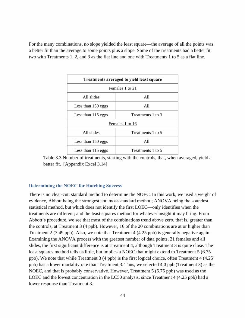
44

For the many combinations, no slope yielded the least square—the average of all the points was a better fit than the average to some points plus a slope. Some of the treatments had a better fit, two with Treatments 1, 2, and 3 as the flat line and one with Treatments 1 to 5 as a flat line.

Treatments averaged to yield least square

Females 1 to 21

All slides All

Less than 150 eggs All

Less than 115 eggs Treatments 1 to 3

Females 1 to 16

All slides Treatments 1 to 5

Less than 150 eggs All

Less than 115 eggs Treatments 1 to 5

Table 3.3 Number of treatments, starting with the controls, that, when averaged, yield a better fit. [Appendix Excel 3.14]

Determining the NOEC for Hatching Success

There is no clear-cut, standard method to determine the NOEC. In this work, we used a weight of evidence, Abbott being the strongest and most-standard method; ANOVA being the soundest statistical method, but which does not identify the first LOEC—only identifies when the treatments are different; and the least squares method for whatever insight it may bring. From Abbott’s procedure, we see that most of the combinations trend above zero, that is, greater than the controls, at Treatment 3 (4 ppb). However, 16 of the 20 combinations are at or higher than Treatment 2 (3.49 ppb). Also, we note that Treatment 4 (4.25 ppb) is generally negative again. Examining the ANOVA process with the greatest number of data points, 21 females and all slides, the first significant difference is at Treatment 4, although Treatment 3 is quite close. The least squares method tells us little, but implies a NOEC that might extend to Treatment 5 (6.75 ppb). We note that while Treatment 3 (4 ppb) is the first logical choice, often Treatment 4 (4.25 ppb) has a lower mortality rate than Treatment 3. Thus, we selected 4.0 ppb (Treatment 3) as the NOEC, and that is probably conservative. However, Treatment 5 (6.75 ppb) was used as the LOEC and the lowest concentration in the LC50 analysis, since Treatment 4 (4.25 ppb) had a lower response than Treatment 3.

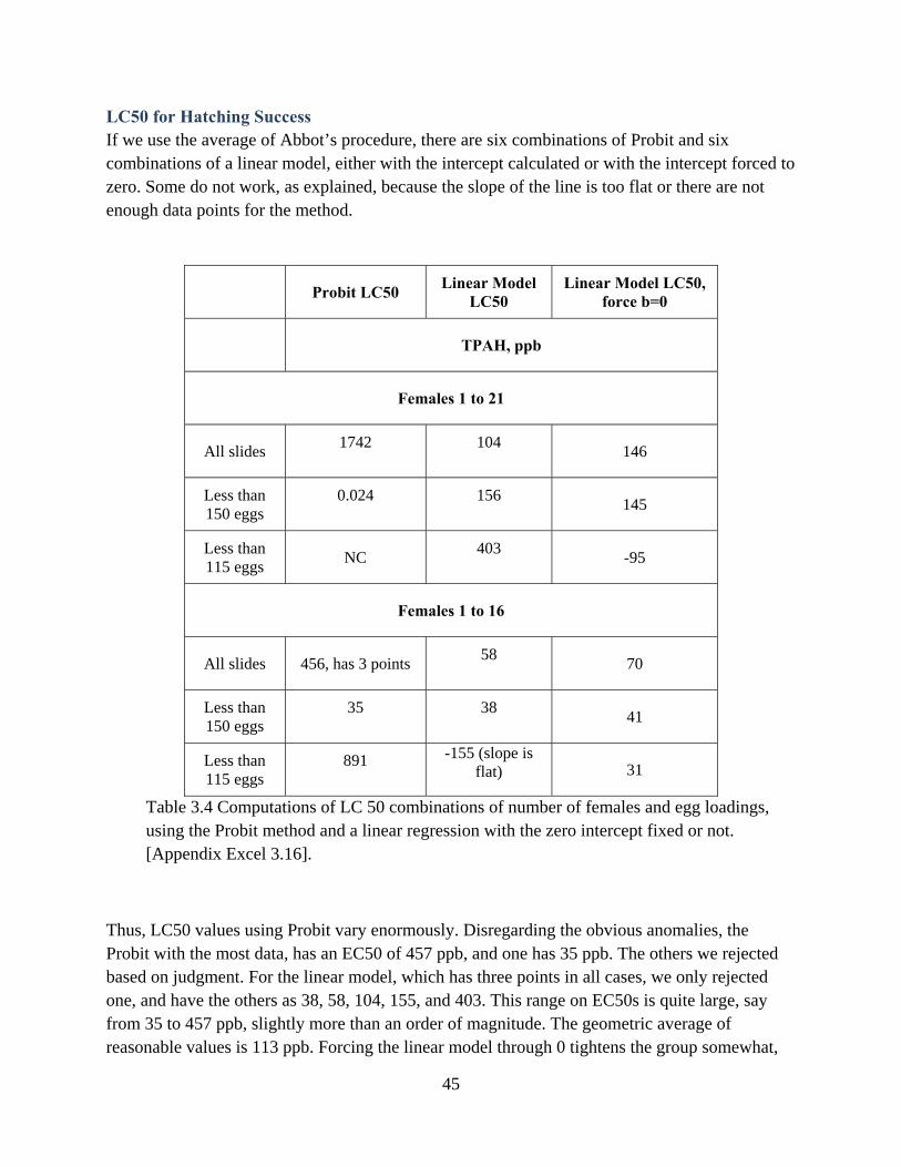
45

LC50 for Hatching Success If we use the average of Abbot’s procedure, there are six combinations of Probit and six combinations of a linear model, either with the intercept calculated or with the intercept forced to zero. Some do not work, as explained, because the slope of the line is too flat or there are not enough data points for the method.

Probit LC50 Linear Model

LC50 Linear Model LC50,

force b=0

TPAH, ppb

Females 1 to 21

All slides 1742

104

146

Less than 150 eggs

0.024

156

145

Less than 115 eggs

NC 403

-95

Females 1 to 16

All slides 456, has 3 points 58

70

Less than 150 eggs

35

38

41

Less than 115 eggs

891

-155 (slope is flat) 31

Table 3.4 Computations of LC 50 combinations of number of females and egg loadings, using the Probit method and a linear regression with the zero intercept fixed or not. [Appendix Excel 3.16].

Thus, LC50 values using Probit vary enormously. Disregarding the obvious anomalies, the Probit with the most data, has an EC50 of 457 ppb, and one has 35 ppb. The others we rejected based on judgment. For the linear model, which has three points in all cases, we only rejected one, and have the others as 38, 58, 104, 155, and 403. This range on EC50s is quite large, say from 35 to 457 ppb, slightly more than an order of magnitude. The geometric average of reasonable values is 113 ppb. Forcing the linear model through 0 tightens the group somewhat,

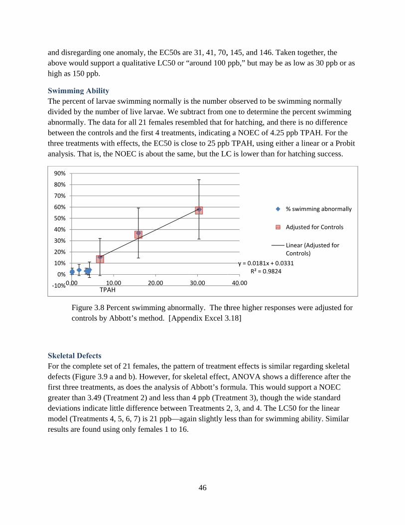
and disreabove wohigh as 1

SwimmiThe percdivided babnormabetween three treaanalysis.

Fco

Skeletal For the cdefects (Ffirst threegreater thdeviationmodel (Tresults ar

‐10%

0%

10%

20%

30%

40%

50%

60%

70%

80%

90%

0.00

egarding oneould support50 ppb.

ng Ability ent of larvae

by the numbelly. The datathe controls

atments withThat is, the

igure 3.8 Peontrols by A

Defects omplete set Figure 3.9 a e treatmentshan 3.49 (Trns indicate liTreatments 4re found usin

0 10.TPAH

e anomaly, tht a qualitativ

e swimming er of live lara for all 21 feand the first

h effects, theNOEC is ab

ercent swimmAbbott’s meth

of 21 femaleand b). How, as does theeatment 2) aittle differenc, 5, 6, 7) is 2ng only fema

.00 2H

he EC50s areve LC50 or “

normally is rvae. We subfemales resemt 4 treatment EC50 is clo

bout the sam

ming abnormhod. [Appen

es, the patterwever, for ske analysis of and less thance between T21 ppb—agaales 1 to 16.

0.00

46

e 31, 41, 70,around 100

the number btract from ombled that fots, indicating

ose to 25 ppbme, but the LC

mally. The thndix Excel 3

rn of treatmekeletal effect

Abbott’s forn 4 ppb (TreaTreatments 2ain slightly le

30.00

, 145, and 14ppb,” but m

observed toone to determfor hatching, g a NOEC ob TPAH, usiC is lower th

hree higher r3.18]

ent effects ist, ANOVA srmula. This atment 3), th2, 3, and 4. Tess than for

y = 0.0181R² = 0

40.00

46. Taken tomay be as low

o be swimmimine the percand there is

of 4.25 ppb Ting either a lhan for hatch

responses w

s similar regshows a diffewould suppo

hough the wiThe LC50 foswimming a

1x + 0.03310.9824

% swim

Adjust

Linear Contro

ogether, the w as 30 ppb o

ng normallycent swimm

s no differencTPAH. For thlinear or a Prhing success

were adjusted

arding skeleerence after ort a NOEC ide standard or the linear ability. Simil

mming abnorm

ed for Control

(Adjusted forols)

or as

y ming

ce he robit .

d for

etal the

lar

mally

s

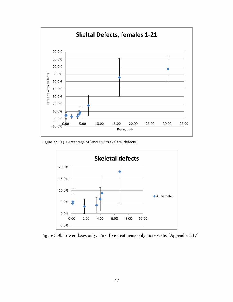
47

Figure 3.9 (a). Percentage of larvae with skeletal defects.

Figure 3.9b Lower doses only. First five treatments only, note scale: [Appendix 3.17]

‐10.0%

0.0%

10.0%

20.0%

30.0%

40.0%

50.0%

60.0%

70.0%

80.0%

90.0%

0.00 5.00 10.00 15.00 20.00 25.00 30.00 35.00

Percent with defects

Dose, ppb

Skeltal Defects, females 1‐21

‐5.0%

0.0%

5.0%

10.0%

15.0%

20.0%

0.00 2.00 4.00 6.00 8.00 10.00

Skeletal defects

All females

48

Comparison with Values in the Literature

Notes on Carls et al. (1999) NOAA researchers exposed herring eggs to effluent water passed over gravel oiled with ANS (Alaska North Slope crude oil). (Carls, Rice et al. 1999) They used two exposure methods: less-weathered oil (LWO) and more-weathered oil (MWO). The chemistry presented indicated a large change in types of PAH in the effluent, the LWO being mostly naphthalenes, and the MWO being mostly chrysenes and phenanthrenes. In addition, for each homologous family, creosote from our experiment was mostly parent PAH, while both the LWO and MWO were mostly alkylated. Of interest here regarding hatching success is that the LWO was not significantly different from the control at about 8 ppb TPAH, with a reported LOEL of 34.3 ppb and with EC50 of 53.3 ppb. This result is about what we have for the creosote TPAH. For MWO, for egg death, the LOEC is 7.61 ppb, about like our numbers. So for both the LWO and the MWO, our putative NOEC of 4 ppb TPAH is conservative. The EC50 of the LWO is within the range of our suggested EC50. Note that the suite of PAHs is quite different between creosote, LWO, and MWO, so it is hard to draw conclusions, other than to say that our results are not inconsistent with those of Carls et al. Regarding other parameters—abnormalities and defects—for those we measured, our data are consistent with or more conservative than the LWO and less conservative than the MWO. A reading of Figure 4 in Carls et al. indicates two sets of control deaths, about 5% in the LWO study and 20% in the MWO study, which were carried out with fish captured at different locations.

Notes on Vines et al. (2000) Vines and team studied the effects of creosote leachate and direct contact with Pacific herring eggs.(Vines, Robbins et al. 2000) A quick reading of the paper would seem to draw conclusions quite different from ours. A close reading of the paper together with our leaching data from Chapter 4 indicates broad agreement.

The first finding of Vines et al. related to eggs scraped from an old piling. This experiment, which appears to be a preliminary and not closely controlled study, found that eggs that remained attached to the piling and were taken to the laboratory (wood pieces were somehow removed from the pile) and kept in seawater did not hatch. Eggs that were scraped off the piling had some hatching success, and eggs scraped from a plastic pipe nearby had high hatching success. It was assumed that the pile was creosote-treated, but details about that were not given. In an email, Dr. Vines told me the pile was not fouled. While this is certainly not uncommon, most old piles are fouled. It is generally assumed that damage to eggs would be more severe early in the gestation. Eggs that were scraped off sometime after spawning would have been damaged already and would have had a mortality rate similar to the eggs remaining on the pile. An alternative explanation for the data is that removal of the wood segments from behind the eggs released creosote from deeper in the wood into the holding water, and this released creosote is what did the damage. The damage did not occur when they were attached to the pile, but while they were being held. The eggs scraped from the pile had about 70% mortality (lack of hatching success).

49

Eggs from nearby (0.4 m, 1 foot) on plastic pipe had low mortality. This section of the Vines et al. paper supports the toxicity of eggs that stick directly to an unfouled pile that had been treated with creosote many years ago, although details of the original treatment or current wood chemistry were not presented, while eggs only about 1 foot away had low mortality.

The second finding in Vines et al. was the exposure of eggs to chemical creosote. That water was measured with instruments, and the concentration of TPAH was measured. We know from our work that the PAH chemistry would vary quite a bit depending on exposure conditions, but presumably naphthalene would leave the water quickly, and naphthalene is a presumed acute toxicant, although there is uncertainty about eggs in that regard. However, Figure 2 in Vines et al. shows an LC50 for hatching success at about 50 ppb TPAH, which is within the range of values we estimated, and what Carls et al. (1999) noted also. (Figure 2 in Vines et al. indicates about 25% mortality in the controls.)

The third finding in Vines et al. (2000) was a list of severe defects associated with incubating the eggs in water with pieces of creosote. The authors found some of these defects varied with salinity and so on. The size of the pieces of treated wood was 1 cm by 8 cm by 0.1 cm. The pieces were placed in a 200 ml dish, but chemistry was not reported. Thus, the TPAH to which the eggs were exposed was not reported, only that the defects occurred in the presence of creosoted wood, under various exposure conditions. Since in our work we determined leaching rates and in two of our treatments we used cut wood, we can estimate the leaching rates in the study. Based on our work, if one applied to that rate to one face of exposed wood and volume of water for one day, the water would have reached a TPAH concentration of 600 ppb. Since the water was changed once a day, that would mean about 300 ppb on average. That rate may be conservative, since the water used in Vines et al. was warmer than ours and less saline, which would increase the leaching rate, although the creosote, even from the freshly cut wood, would be old and perhaps less mobile than creosote from new wood. Applying the 300 ppb dose to the data in Figure 2 of Vines et al. would indicate only an 8% hatching success rate. Thus, our general conclusion that the LC50 is about 100 ppb and may be as low as 50 ppb in not in conflict with the Vines et al. findings.

Conclusions

Despite the issue with high control deaths and large variances in our data, the very large amount of data enables us to estimate toxicity with some confidence. The NOEC is somewhere between 3.5 and 6.5 ppb. We recommend 4 ppb as a value that is probably conservative. The LC50 for hatching success is somewhere between 30 and 150 ppb, while the EC50 for both swimming ability and skeletal defects is more definite, about 25 ppb. The statistical analysis reported in the Appendix reports a more conservative numbers for EC50 for the hatching success and approximately the same numbers for skeletal defects and swimming ability.

50

Chapter 4. Exposure Assessment

Introduction

Exposure evaluations are descriptions of the release, fate, and transportation of contaminants into the environment—in this case marine water. Specifically, we are evaluating the concentration of PAH chemicals herring eggs may experience both from new BMP piles and from older non-BMP piles. Recognizing the difficulty and uncertainty involved with predicting these concentrations, we used several methods to evaluate exposure and presented a range of reasonable values: literature values, direct measuring, and modeling. The direct measuring techniques were to evaluate the concentrations directly from reported literature, our direct field, laboratory measurements, and our field LDPE. The field measurements near installed piles were very low; the LDPE measurements required non-standardize calculations in order to extrapolate the data to achieve estimates of water concentrations. The modeling techniques used estimated exposure concentrations based on leaching rates reported and measured in our lab. We then calculated concentrations in the water column based on field and reported values for currents. Again, while some of these calculations are standard for idealized situations, they needed site-specific modifications.

Most of the literature regarding creosote contamination refers to PAH concentrations in sediment. Much less information is available regarding PAH concentrations in the water column. Besides literature that reports direct values in the water and sediment, we found literature that reports leaching rates. Literature often reports results from waters of different temperature and salinity than those of Alaska, as well as from wood species different from those used in Alaska, and thus some judgment is needed about using values as they are, or converting them by mathematic models to Alaskan conditions. Regarding values reported in the literature, some of the older instrumentation reported results in ppm, while we learned that there are effects at the low ppb range. Nonetheless, we found some values reported at the low ppb range in the literature.

For new piles, there are models that predict the rate of loss starting with retention of creosote. These models generally relate to creosote as an entity, rather than to creosote’s PAH chemicals. For new BMP piles, the minimum specified retention is known. The actual retention varies somewhat and may be above that minimum retention when the pile is shipped from the treater. Some of the more volatile components are lost during the treating, shipping processes, and storage.

Leaching Rate Results

Our Laboratory

Method The rate of PAH transfer from creosote-treated wood to the surrounding water is referred to as the “leaching rate” and reported as micrograms of chemical per square centimeter per day

51

(g/cm2/day). For each of the 7 treatments, we measured the flow of water through the generator columns and the concentrations of TPAH in the effluent water. The Appendix has photographs and some details. Here we summarize: For this study, we used creosote-treated lumber supplied by Baxter (see Acknowledgements), with the support of Oregon State University (OSU; see

Acknowledgments.). The uncut lumber pieces were 26 nominal (50.8 mm x 152.4 mm), two feet (61 cm) long, treated to 25 pcf (pounds per cubic foot, 400 kg/m3), and finished to BMP. All of the pieces were originally end-sealed by OSU with epoxy before treatment. After receipt, we sealed both ends of the piece with epoxy and a piece of un-treated wood cap. However as herring spawning season approached and the sealed pieces were not releasing sufficient TPAH, we cut some of the pieces to speed PAH release. Treatments 1, 2, and 3 had two cut ends; several boards in Treatment 7 were also cut. For example, Treatment 1, a piece 2 inches long, had a large proportion of its surface area freshly exposed by cutting. We discuss the difference in PAH species between the cut and uncut lumber in Chapter 2, but there was not enough difference to warrant an approach different from using TPAH as the dose in our toxicity tests.

Because of the uncertainty of the start of herring spawning, the pre-leach was carried out before the start of the tox testing. The lumber was first pre-leached with flowing seawater either in a large plastic garbage can or in a PVC tube. The TPAH reported for this leaching rate study was measured with GC/MS. (Parallel studies of PAH were done with a UV meter for real-time analysis to adjust flow rates and wood loading, although this method has much lower resolution than GC/MS.) Thus, we obtained a data set for leaching rates for this pre-leach. Flow rates were measured, recorded, and adjusted as needed. Although PAH may cling to PVC and plastic, we measured the PAH concentrations in the well-mixed effluent water.

After this 28-day pre-leach step, the boards were sealed in plastic, placed in cold storage for 10 days, and then, as spawning approached, placed into the PVC generator columns. For about 21 days the boards were in flowing seawater, but various combinations of boards and flow rates were utilized. As the flow rates were adjusted and UV indicated insufficient PAH was being generated, cut boards and un-leached boards were utilized to increase PAH. Note that Treatment 7 used all un-leached boards, so we have included that data in the pre-leaching study. We do not have GC measurements for this preliminary adjustment period. Table 4.1 gives a summary of the boards in each generator column.

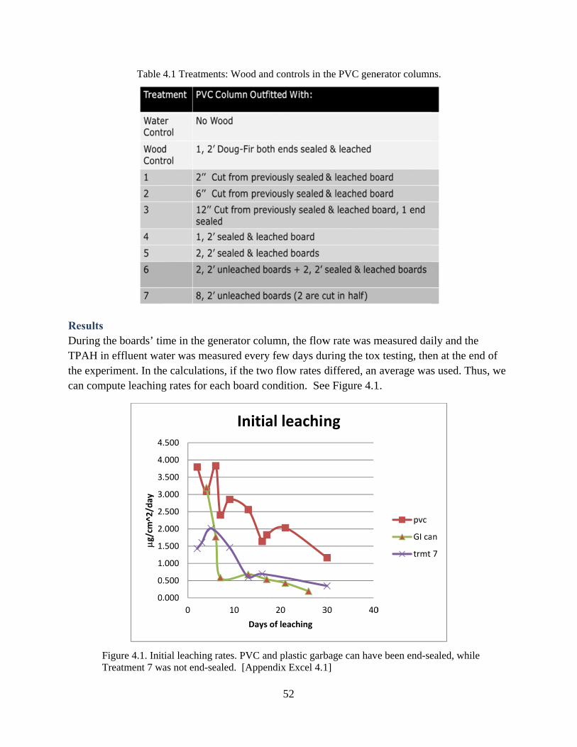
Results During thTPAH inthe expercan comp

FT

Table

he boards’ tin effluent wariment. In thpute leaching

igure 4.1. InitTreatment 7 w

0

0

1

1

2

2

3

3

4

4

g/cm^2/day

4.1 Treatmen

ime in the geater was meahe calculationg rates for ea

tial leaching rwas not end-se

0.000

0.500

.000

.500

.000

.500

.000

.500

4.000

4.500

0

nts: Wood and

enerator coluasured every ns, if the twoach board co

rates. PVC anealed. [Appen

10

Days o

Initia

52

d controls in t

umn, the flowfew days du

o flow rates ondition. Se

nd plastic garbndix Excel 4.1

20 3

of leaching

al leachi

the PVC gene

w rate was muring the toxdiffered, an

ee Figure 4.1

bage can have1]

30 40

ng

erator column

measured daix testing, theaverage was

1.

e been end-se

0

pvc

GI ca

trmt 

ns.

ily and the en at the end s used. Thus

ealed, while

n

7

of s, we

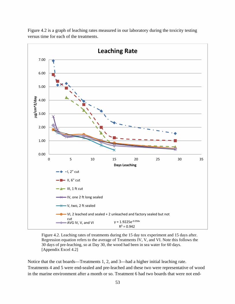
53

Figure 4.2 is a graph of leaching rates measured in our laboratory during the toxicity testing versus time for each of the treatments.

Figure 4.2. Leaching rates of treatments during the 15 day tox experiment and 15 days after. Regression equation refers to the average of Treatments IV, V, and VI. Note this follows the 30 days of pre-leaching, so at Day 30, the wood had been in sea water for 60 days. [Appendix Excel 4.2]

Notice that the cut boards—Treatments 1, 2, and 3—had a higher initial leaching rate. Treatments 4 and 5 were end-sealed and pre-leached and these two were representative of wood in the marine environment after a month or so. Treatment 6 had two boards that were not end-

y = 1.9225e‐0.058x

R² = 0.942

0.00

1.00

2.00

3.00

4.00

5.00

6.00

7.00

0 5 10 15 20 25 30 35

g/cm^2/day

Days Leaching

Leaching Rate

I, 2" cut

II, 6" cut

III, 1 ft cut

IV, one 2 ft long sealed

V, two, 2 ft sealed

VI, 2 leached and sealed + 2 unleached and factory sealed but notcutAVG IV, V, and VI

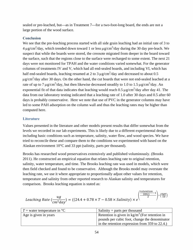
54

sealed or pre-leached, but—as in Treatment 7—for a two-foot-long board, the ends are not a large portion of the wood surface.

Conclusion We see that the pre-leaching process started with all side grain leaching had an initial rate of 3 to

4 g/cm2/day, which trended down toward 1 or less g/cm2/day during the 30 day pre-leach. We suspect that while the boards were stored, the creosote migrated from deeper in the board toward the surface, such that the regions close to the surface were recharged to some extent. The next 21 days were not monitored for TPAH and the water conditions varied somewhat. For the generator columns of treatments IV and V, which had all end-sealed boards, and including VI, which has

half end-sealed boards, leaching resumed at 2 to 3 g/cm2/day and decreased to about 0.5

g/cm2/day after 30 days. On the other hand, the cut boards that were not end-sealed leached at a

rate of up to 7 g/cm2/day, but then likewise decreased steadily to 1.0 to 1.5 g/cm2/day. An

exponential fit of that data indicates that leaching would reach 0.5 g/cm2/day after day 41. The data from our laboratory testing indicated that a leaching rate of 1.0 after 30 days and 0.5 after 60 days is probably conservative. Here we note that use of PVC in the generator columns may have led to some PAH adsorption on the column wall and thus the leaching rates may be higher than computed here.

Literature

Values presented in the literature and other models present results that differ somewhat from the levels we recorded in our lab experiments. This is likely due to a different experimental design including basic conditions such as temperature, salinity, water flow, and wood species. We have tried to reconcile these and compare them to the conditions we experimented with based on the Alaskan environment 10°C and 33 ppt (salinity, parts per thousand).

Brooks has researched wood preservatives extensively and published voluminously. (Brooks 2011). He constructed an empirical equation that relates leaching rate to original retention, salinity, water temperature, and time. The Brooks leaching rate was used in models, which were then field checked and found to be conservative. Although the Brooks model may overstate the leaching rate, we use it where appropriate to proportionally adjust other values for retention, temperature and salinity from other reported research to Alaskan salinity and temperatures for comparison. Brooks leaching equation is stated as:

24.4 0.78 0.58

.

T = water temperature in °C Salinity = parts per thousand Age is given in years Retention is given in kg/m3 (For retention in

pounds per cubic foot, change the denominator in the retention expression from 359 to 22.4.)

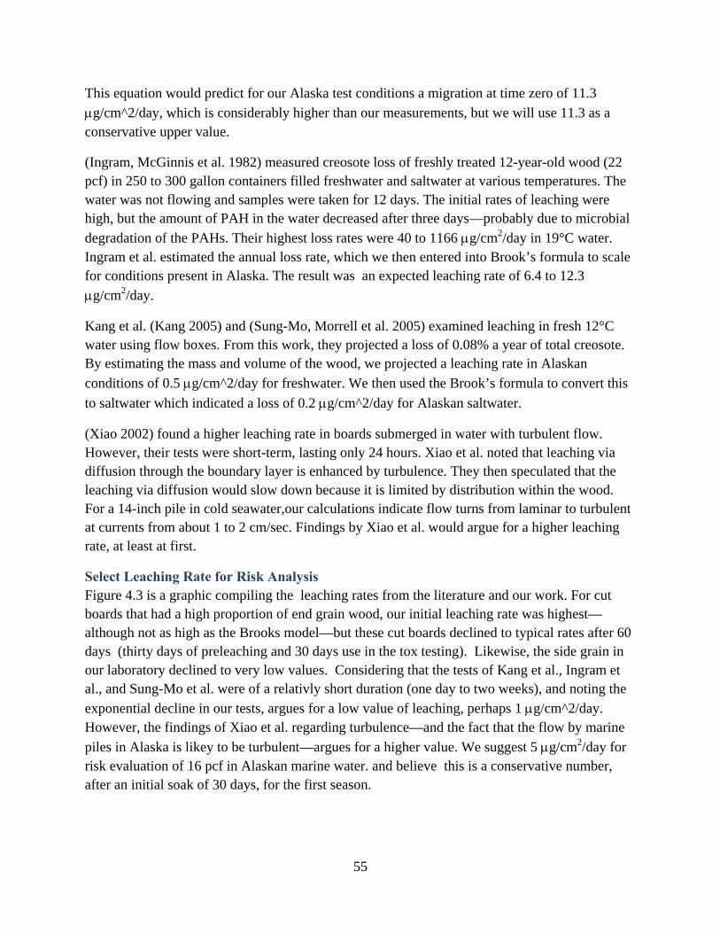
55

This equation would predict for our Alaska test conditions a migration at time zero of 11.3

g/cm^2/day, which is considerably higher than our measurements, but we will use 11.3 as a conservative upper value.

(Ingram, McGinnis et al. 1982) measured creosote loss of freshly treated 12-year-old wood (22 pcf) in 250 to 300 gallon containers filled freshwater and saltwater at various temperatures. The water was not flowing and samples were taken for 12 days. The initial rates of leaching were high, but the amount of PAH in the water decreased after three days—probably due to microbial

degradation of the PAHs. Their highest loss rates were 40 to 1166 g/cm2/day in 19°C water. Ingram et al. estimated the annual loss rate, which we then entered into Brook’s formula to scale for conditions present in Alaska. The result was an expected leaching rate of 6.4 to 12.3

g/cm2/day.

Kang et al. (Kang 2005) and (Sung-Mo, Morrell et al. 2005) examined leaching in fresh 12°C water using flow boxes. From this work, they projected a loss of 0.08% a year of total creosote. By estimating the mass and volume of the wood, we projected a leaching rate in Alaskan

conditions of 0.5 g/cm^2/day for freshwater. We then used the Brook’s formula to convert this

to saltwater which indicated a loss of 0.2 g/cm^2/day for Alaskan saltwater.

(Xiao 2002) found a higher leaching rate in boards submerged in water with turbulent flow. However, their tests were short-term, lasting only 24 hours. Xiao et al. noted that leaching via diffusion through the boundary layer is enhanced by turbulence. They then speculated that the leaching via diffusion would slow down because it is limited by distribution within the wood. For a 14-inch pile in cold seawater,our calculations indicate flow turns from laminar to turbulent at currents from about 1 to 2 cm/sec. Findings by Xiao et al. would argue for a higher leaching rate, at least at first.

Select Leaching Rate for Risk Analysis Figure 4.3 is a graphic compiling the leaching rates from the literature and our work. For cut boards that had a high proportion of end grain wood, our initial leaching rate was highest—although not as high as the Brooks model—but these cut boards declined to typical rates after 60 days (thirty days of preleaching and 30 days use in the tox testing). Likewise, the side grain in our laboratory declined to very low values. Considering that the tests of Kang et al., Ingram et al., and Sung-Mo et al. were of a relativly short duration (one day to two weeks), and noting the

exponential decline in our tests, argues for a low value of leaching, perhaps 1 g/cm^2/day. However, the findings of Xiao et al. regarding turbulence—and the fact that the flow by marine

piles in Alaska is likey to be turbulent—argues for a higher value. We suggest 5 g/cm2/day for risk evaluation of 16 pcf in Alaskan marine water. and believe this is a conservative number, after an initial soak of 30 days, for the first season.

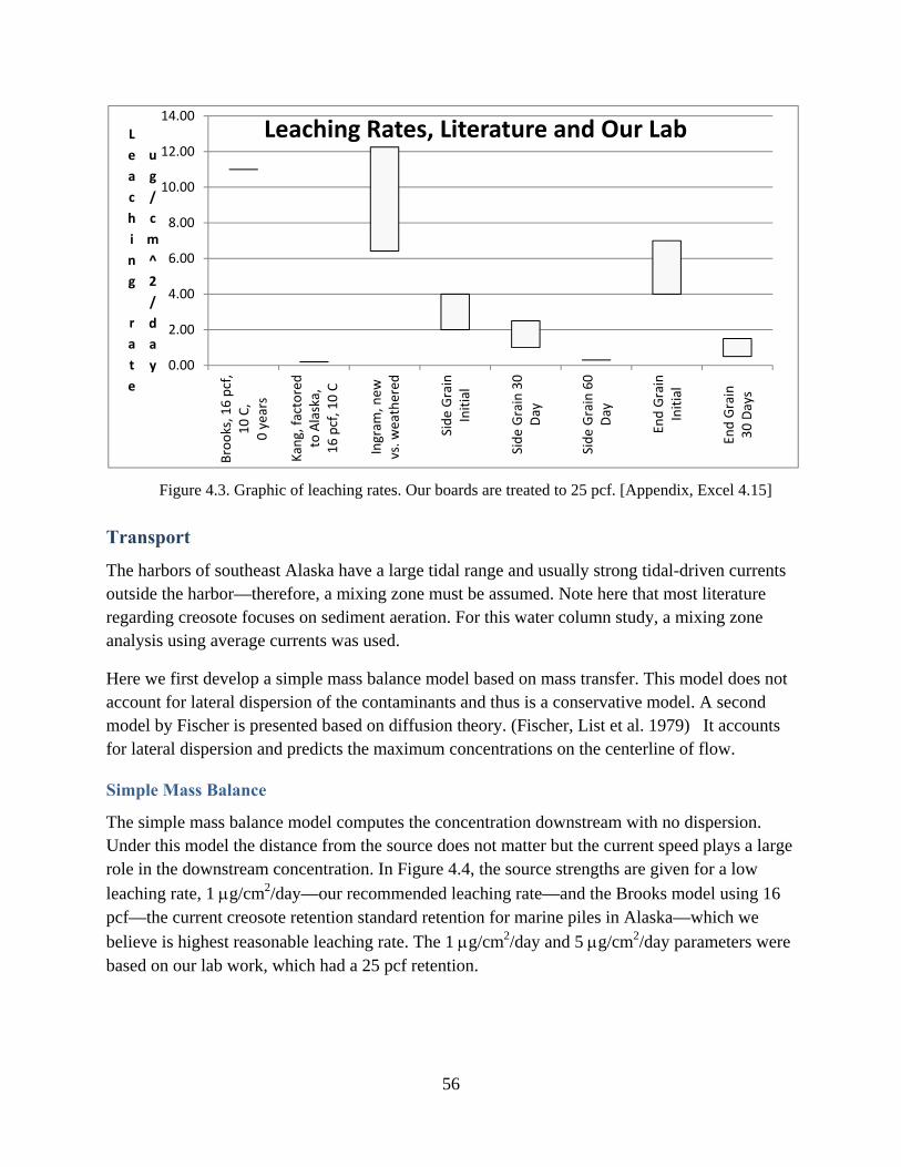
56

Figure 4.3. Graphic of leaching rates. Our boards are treated to 25 pcf. [Appendix, Excel 4.15]

Transport

The harbors of southeast Alaska have a large tidal range and usually strong tidal-driven currents outside the harbor—therefore, a mixing zone must be assumed. Note here that most literature regarding creosote focuses on sediment aeration. For this water column study, a mixing zone analysis using average currents was used.

Here we first develop a simple mass balance model based on mass transfer. This model does not account for lateral dispersion of the contaminants and thus is a conservative model. A second model by Fischer is presented based on diffusion theory. (Fischer, List et al. 1979) It accounts for lateral dispersion and predicts the maximum concentrations on the centerline of flow.

Simple Mass Balance

The simple mass balance model computes the concentration downstream with no dispersion. Under this model the distance from the source does not matter but the current speed plays a large role in the downstream concentration. In Figure 4.4, the source strengths are given for a low

leaching rate, 1 g/cm2/day—our recommended leaching rate—and the Brooks model using 16 pcf—the current creosote retention standard retention for marine piles in Alaska—which we

believe is highest reasonable leaching rate. The 1 g/cm2/day and 5 g/cm2/day parameters were based on our lab work, which had a 25 pcf retention.

0.00

2.00

4.00

6.00

8.00

10.00

12.00

14.00

Brooks, 16 pcf,

10 C,

0 years

Kang, factored

to Alaska,

16 pcf, 10 C

Ingram

, new

vs. w

eathered

Side Grain

Initial

Side Grain 30

Day

Side Grain 60

Day

End Grain

Initial

End Grain

30 Days

L

e

a

c

h

i

n

g

r

a

t

e

u

g

/

c

m

^

2

/

d

a

y

Leaching Rates, Literature and Our Lab

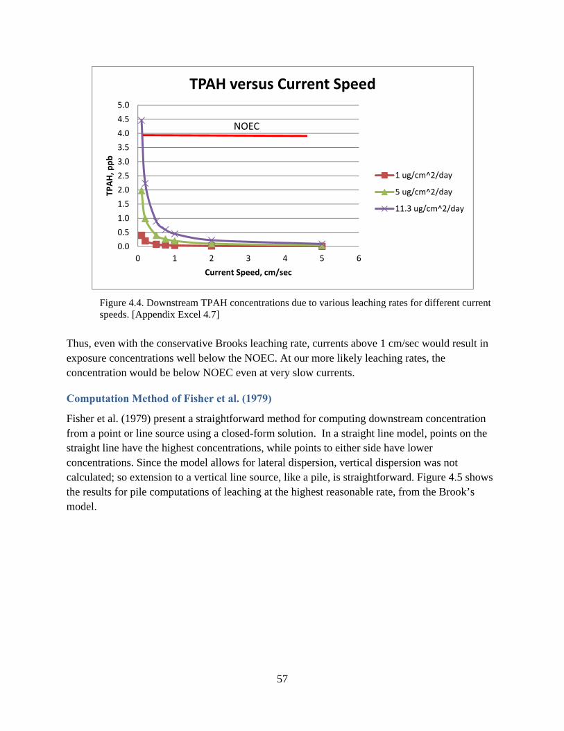
57

Figure 4.4. Downstream TPAH concentrations due to various leaching rates for different current speeds. [Appendix Excel 4.7]

Thus, even with the conservative Brooks leaching rate, currents above 1 cm/sec would result in exposure concentrations well below the NOEC. At our more likely leaching rates, the concentration would be below NOEC even at very slow currents.

Computation Method of Fisher et al. (1979)

Fisher et al. (1979) present a straightforward method for computing downstream concentration from a point or line source using a closed-form solution. In a straight line model, points on the straight line have the highest concentrations, while points to either side have lower concentrations. Since the model allows for lateral dispersion, vertical dispersion was not calculated; so extension to a vertical line source, like a pile, is straightforward. Figure 4.5 shows the results for pile computations of leaching at the highest reasonable rate, from the Brook’s model.

0.0

0.5

1.0

1.5

2.0

2.5

3.0

3.5

4.0

4.5

5.0

0 1 2 3 4 5 6

TPAH, p

pb

Current Speed, cm/sec

TPAH versus Current Speed

1 ug/cm^2/day

5 ug/cm^2/day

11.3 ug/cm^2/day

NOEC

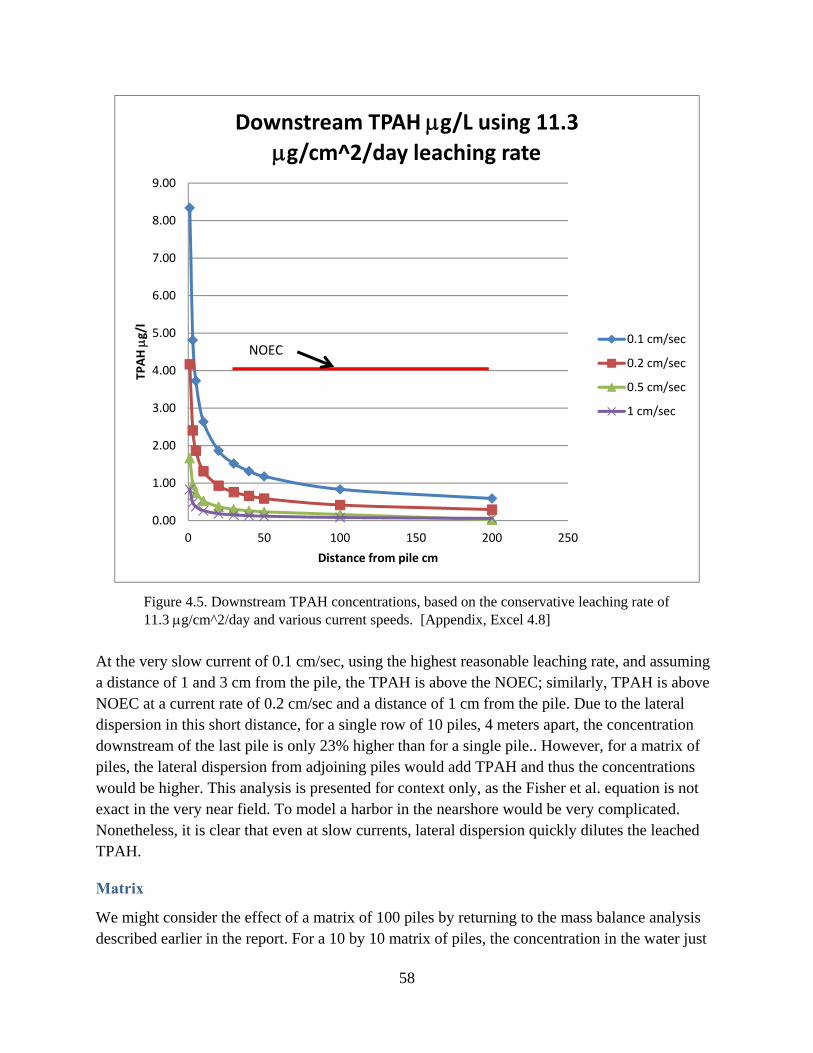
58

Figure 4.5. Downstream TPAH concentrations, based on the conservative leaching rate of 11.3 g/cm^2/day and various current speeds. [Appendix, Excel 4.8]

At the very slow current of 0.1 cm/sec, using the highest reasonable leaching rate, and assuming a distance of 1 and 3 cm from the pile, the TPAH is above the NOEC; similarly, TPAH is above NOEC at a current rate of 0.2 cm/sec and a distance of 1 cm from the pile. Due to the lateral dispersion in this short distance, for a single row of 10 piles, 4 meters apart, the concentration downstream of the last pile is only 23% higher than for a single pile.. However, for a matrix of piles, the lateral dispersion from adjoining piles would add TPAH and thus the concentrations would be higher. This analysis is presented for context only, as the Fisher et al. equation is not exact in the very near field. To model a harbor in the nearshore would be very complicated. Nonetheless, it is clear that even at slow currents, lateral dispersion quickly dilutes the leached TPAH.

Matrix

We might consider the effect of a matrix of 100 piles by returning to the mass balance analysis described earlier in the report. For a 10 by 10 matrix of piles, the concentration in the water just

0.00

1.00

2.00

3.00

4.00

5.00

6.00

7.00

8.00

9.00

0 50 100 150 200 250

TPAH g/l

Distance from pile cm

Downstream TPAH g/L using 11.3 g/cm^2/day leaching rate

0.1 cm/sec

0.2 cm/sec

0.5 cm/sec

1 cm/sec

NOEC

59

downstream of the tenth pile in the column would be tenfold greater than the concentration just downstream of the first pile. If the 14-inch piles were spaced 4 meters apart and the contamination were distributed evenly, each pile would have 2 meters on each side. If the downstream contamination were spread into that area, the dilution factor would be 14 inches/4 meters or 9.4%. Thus, the additive effect of piles in a column would be canceled by sideward dispersion. Of course, dispersion is not instant and we cannot calculate the near field, but some distance from the matrix, the concentrations are again far below the NOEC. In the near field—under the structure or very close to it—concentrations could approach the NOEC, at least for large newly installed structures in slow currents. Consequently, these would be the subject of a risk assessment if the area under the structure cannot be subtracted from the habitat.

Currents

The currents used in a risk analysis model should be site-specific and typically use currents at the structure under consideration. But here we must generalize. Alaska marine harbors have strong tidal currents. Estuarine harbors might have river flow as well, but in most Alaska saltwater locations, the tidal currents are much greater than river flow. We measured the current velocity at three Juneau-area harbors: Otter Way/Indian Cove National Park Service, Auke Bay Marine Site, and Aurora Harbor (see Appendix Excel 4.9 and 4.10). In general, we are interested in the average current somewhere in the water column that minimizes surface and bottom effects. The average current we measured was between 2 and 2.5 cm/sec. This average includes measurements taken close to shore and at the end of docks. Longer-term measurements with anchored meters at the bottom in the nearshore Juneau locations indicated currents of 2.15 to 5.72 cm/sec [Appendix Excel 4.11](Stone 2003). Note that these currents contrast with those offshore in the channels, where the average current is often over 20 cm/sec at 20 foot depth [Appendix Excel 4.12] (NOAA 2008). Using a current speed of 2 cm/sec, therefore, is slightly conservative. Certainly, for an average current in southeast Alaska harbors of 1 cm/sec is conservative, and we use that in our risk calculations.

Field Measurements.

We made some TPAH measurements for direct consideration and also to compare them to the source and transport models.

A. Laboratory. During the toxicity experiments, we measured PAH concentrations using traditional extraction of the water. With the LDPE method, we had LDPE samplers in each of the treatment waters. We estimated the concentration of creosote in the timbers based on the reported retention and the actual values from similar wood specimens.

B. Field. We measured PAH concentrations in three locations known to have creosoted timbers in harbors near Juneau, Alaska, both directly and by LDPE. Of the nine direct samples, seven were in the several hundred parts per trillion (pptr) range (average 314 ppt), while two were in the low parts per billion (ppb). However these two samples, both from National Park

60

Service dock (NPS), were likely compromised because the researcher roiled the sediment while taking the samples and thus the samples likely contained sediment particles. [Appendix Excel 4.21]

C. LDPE. Low-density polyethylene plastic (LDPE) has a high affinity for hydrocarbons and rapidly extracts them from water. The theory and chemistry of LDPE is similar to that of semi-permeable membrane devices (SPMD), and there is much more literature about SPMD than LDPE. The chief difference between them is that SPMD has a lipophilic chemical inside a polyethylene tube—which absorbs most of the hydrocarbon—while LDPE has no “filling” and the tube itself is in an absorbing medium. Both SPMD and LDPE are proven to extract even very low concentrations of hydrocarbons from the water and sequester them, which allows for later extraction and analysis typically by GC/MS. Both SPMD and LDPE remain in the water days or weeks, which integrates and concentrates the chemicals over time. Also, both have proven their value to distinguishing which chemicals are in the water and for differentiating chemicals from different locations and sources. The U.S. Geological Survey has a web site with an excellent overview of SPMD technology. (Huckins, Petty et al. 2012) and Carls has an introduction to LDPE and a comparison to SPMDs. (Carls, Holland et al. 2004) Both SPMD and LDPE report their findings as mass of chemical per mass of membrane and there is no exact method to translate this into concentration, mass per volume of water though several models purport to do so. In our tox experiments—modeled after Durrell, Row Utvik et all.—we placed LDPE devices in the effluent water for each treatment, a 0.33 gm sampler for the first 15 days and a 1.1 gm sampler for the next 15 days. Since we have GC/MS data, we know the average PAH concentrations the devices experienced. With some insight into the operation of LDPEs, we can use this data to estimate concentrations in situ.

Several general issues must be examined in order to estimate environmental concentrations of contaminant PAHs from the mass of contaminants in the LDPE. The first issue is whether the permeability of the membrane is the same for all PAH species. The second issue is determining the contact rate or the volume of water from which all the contaminants is removed.

The sampling rate in liters/ day, “Rs,” allows conversion of mass of chemical in the LDPE sampler to concentration in the water. One can determine Rs for TPAH or for any component PAH. Certainly Rs depends on the sampling time, Kow of the PAH compounds, temperature, water currents, and other parameters. Rather than attempt a theoretical computation of Rs, we used the data from our lab experiments. In Appendix Excel 4.18, we examine the Rs for each species and note some anomalies. Since we are using TPAH as the measurement of exposure, we will use this as the base for our risk assessment.

Based on our lab work, the Rs for TPAH varied. Rs was higher on Days 1 to 15, when the concentrations were higher and the samplers smaller (0.33 gm), and Days 15 to 30, when the concentrations were lower and the samplers larger (1.1 gm). The two sets average 0.91 L/gm day. [Appendix Excel 4.19] That Rs, 0.91 L/gm/day, is close to that of Luellen and Shea and

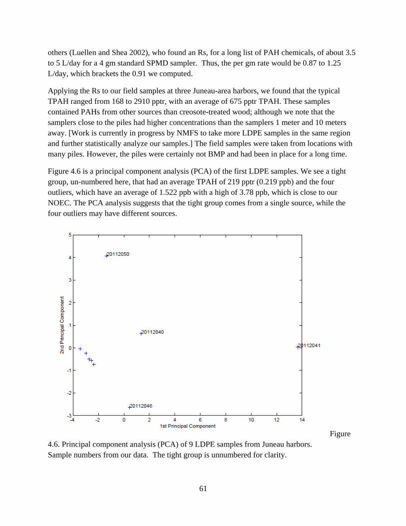
61

others (Luellen and Shea 2002), who found an Rs, for a long list of PAH chemicals, of about 3.5 to 5 L/day for a 4 gm standard SPMD sampler. Thus, the per gm rate would be 0.87 to 1.25 L/day, which brackets the 0.91 we computed.

Applying the Rs to our field samples at three Juneau-area harbors, we found that the typical TPAH ranged from 168 to 2910 pptr, with an average of 675 pptr TPAH. These samples contained PAHs from other sources than creosote-treated wood; although we note that the samplers close to the piles had higher concentrations than the samplers 1 meter and 10 meters away. [Work is currently in progress by NMFS to take more LDPE samples in the same region and further statistically analyze our samples.] The field samples were taken from locations with many piles. However, the piles were certainly not BMP and had been in place for a long time.

Figure 4.6 is a principal component analysis (PCA) of the first LDPE samples. We see a tight group, un-numbered here, that had an average TPAH of 219 pptr (0.219 ppb) and the four outliers, which have an average of 1.522 ppb with a high of 3.78 ppb, which is close to our NOEC. The PCA analysis suggests that the tight group comes from a single source, while the four outliers may have different sources.

Figure 4.6. Principal component analysis (PCA) of 9 LDPE samples from Juneau harbors. Sample numbers from our data. The tight group is unnumbered for clarity.

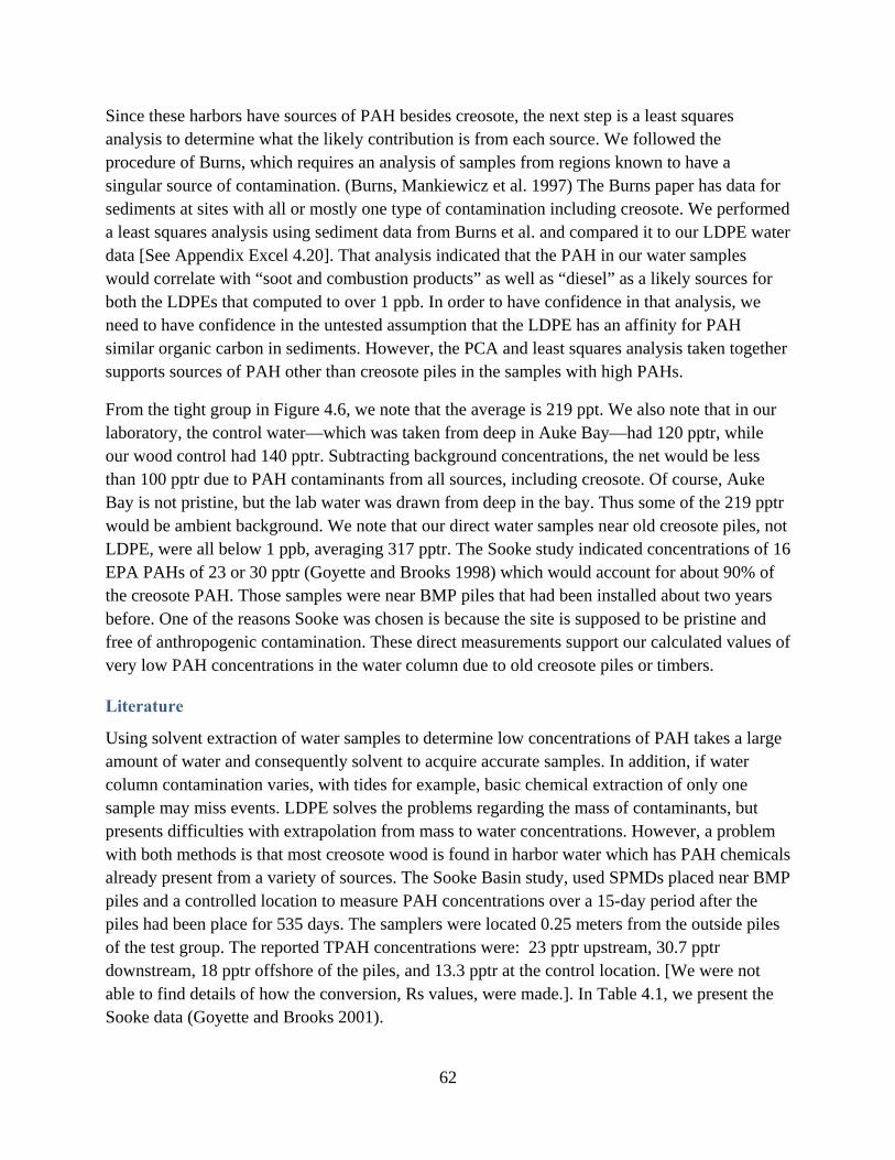
62

Since these harbors have sources of PAH besides creosote, the next step is a least squares analysis to determine what the likely contribution is from each source. We followed the procedure of Burns, which requires an analysis of samples from regions known to have a singular source of contamination. (Burns, Mankiewicz et al. 1997) The Burns paper has data for sediments at sites with all or mostly one type of contamination including creosote. We performed a least squares analysis using sediment data from Burns et al. and compared it to our LDPE water data [See Appendix Excel 4.20]. That analysis indicated that the PAH in our water samples would correlate with “soot and combustion products” as well as “diesel” as a likely sources for both the LDPEs that computed to over 1 ppb. In order to have confidence in that analysis, we need to have confidence in the untested assumption that the LDPE has an affinity for PAH similar organic carbon in sediments. However, the PCA and least squares analysis taken together supports sources of PAH other than creosote piles in the samples with high PAHs.

From the tight group in Figure 4.6, we note that the average is 219 ppt. We also note that in our laboratory, the control water—which was taken from deep in Auke Bay—had 120 pptr, while our wood control had 140 pptr. Subtracting background concentrations, the net would be less than 100 pptr due to PAH contaminants from all sources, including creosote. Of course, Auke Bay is not pristine, but the lab water was drawn from deep in the bay. Thus some of the 219 pptr would be ambient background. We note that our direct water samples near old creosote piles, not LDPE, were all below 1 ppb, averaging 317 pptr. The Sooke study indicated concentrations of 16 EPA PAHs of 23 or 30 pptr (Goyette and Brooks 1998) which would account for about 90% of the creosote PAH. Those samples were near BMP piles that had been installed about two years before. One of the reasons Sooke was chosen is because the site is supposed to be pristine and free of anthropogenic contamination. These direct measurements support our calculated values of very low PAH concentrations in the water column due to old creosote piles or timbers.

Literature

Using solvent extraction of water samples to determine low concentrations of PAH takes a large amount of water and consequently solvent to acquire accurate samples. In addition, if water column contamination varies, with tides for example, basic chemical extraction of only one sample may miss events. LDPE solves the problems regarding the mass of contaminants, but presents difficulties with extrapolation from mass to water concentrations. However, a problem with both methods is that most creosote wood is found in harbor water which has PAH chemicals already present from a variety of sources. The Sooke Basin study, used SPMDs placed near BMP piles and a controlled location to measure PAH concentrations over a 15-day period after the piles had been place for 535 days. The samplers were located 0.25 meters from the outside piles of the test group. The reported TPAH concentrations were: 23 pptr upstream, 30.7 pptr downstream, 18 pptr offshore of the piles, and 13.3 pptr at the control location. [We were not able to find details of how the conversion, Rs values, were made.]. In Table 4.1, we present the Sooke data (Goyette and Brooks 2001).

63

Compound/ Device

BMP Downstream

BMP Upstream

BMP Offshore

Open Control

Naphthalene 6.47 7.16 5.44 5.04 Acenaphthalene 0.54 0.64 0.60 0.44 Acenaphthene 4.62 7.16 3.11 2.13 Fluorene 3.69 4.57 2.78 1.99 Phenanthrene 4.06 5.67 2.85 2.03 Anthracene 0.46 0.70 0.44 0.09 Fluoranthene 2.40 3.69 2.07 1.39 Pyrene 0.57 0.94 0.46 0.21 benz(a)anthracene 0.04 0.07 0.03 0.002 Chrysene 0.03 0.06 0.03 0.001 Benzofluoranthenes 0.01 0.02 0.02 0.016 benzo(a)pyrene 0.003 0.006 0.003 0.002 dibenz(ah)anthracene 0.003 0.002 0.002 0.001 ideno(1,2,3-cd)pyrene 0.002 0.006 0.006 0.001 benzo(ghi)perylene 0.006 0.010 0.007 0.003 Total PAH 22.94 30.76 17.86 13.37

Note: All values are in ng/L (parts per trillion).

Table 4.1. Reproduced from the Sooke Basin report (Goyette and Brooks 1998), where it is Table 11. Dissolved PAH in the water at a distance of 0.25 meters from perimeter piling at the Best Management Practices creosote treated dolphin at the Sooke Basin Creosote Evaluation Study site. Although these data are only for parent PAH, we note that our data indicates alkylated PAH was only 9% of TPAH. Since the “offshore” and “open control” samples are essentially control samples, these could be subtracted from the two near the BMP pile to yield a TPAH of about 15 pptr due to the piles. These values are very low, but are consistent with our findings of direct water samples, most of which were a few hundred parts per trillion, if our known background from Auke Bay is subtracted.

64

Conclusions

For long-term leaching in Alaskan harbors, based on our measured leaching rates and average current velocities in three harbors and computed dilutions, it is unlikely that new BMP creosote piles significantly increase the TPAH in the water column—the increases are most likely well below the NOEC of 4,000 ppt. That colculsion is supported by:

The literature on the data at the Sooke locations indicate TPAH near creosote piles at levels in the range of parts per trillion—far below the NOEC.

The measured water TPAH concentrations in 7 of our 9 harbor samples were low, a few hundred pptr.

Our measured leaching rate and most-conservative reasonable leaching rate and the most-conservative mass balance model indicates concentrations of TPAH in the water well below the NOEC at current speeds which are slower than the current speeds in most Alaskan harbors.

At the highest reasonable leaching rate, a more-accurate model that accounts for lateral dispersion indicates concentrations below the NOEC only a few centimeters from the pile. Although the model is not definitive in the near field, it supports very low concentrations downstream from creosote applications.

The LDPE data translated by our estimated value of Rs indicates TPAH at an average of 219 pptr for the 5 of the 9 samples, which principal component analysis indicates have similar chemistry. (The other 4 samples, which PCA indicates are outliers, have varied chemistry and a preliminary analysis indicated that other contaminants such as diesel and atmospheric soot are likely present and factoring into TPAH measurements.)

65

Chapter 5. ACZA

In general, the water-based wood preservatives chromated copper arsenate (CCA) and ammoniacal copper zinc arsenate (ACZA) are considered less toxic than creosote (Poston 2001). They release copper and other metals into the marine environment, but the effects of CCA and ACZA are considered by some agencies to be less harmful to the environment than the effects of creosote. The EPA considers both ACZA and creosote acceptable for use in marine waters. CCA is more commonly used nationwide but CCA does not penetrate well into Douglas fir which is the wood species most often used in Alaska. The wood preservative most commonly used to treat Douglas fir in Alaska is ACZA. In this chapter, we will briefly examine the relative toxicity of creosote versus ACZA, but focus on the characteristics of ACZA applicable to its use in Alaskan marine waters. We are working towards guiding management decisions based on a balance of the relative costs and benefits at particular projects, while not endorsing particular products.

In comparing creosote with ACZA, the toxicity of PAH is assumed to relate to its activation in animals, both vertebrates and invertebrates, to more reactive imetabolites. These in turn may attach to tissues and perhaps cellular DNA where adducts may cause cancer or genetic anomalies. Since PAH is ubiquitous in the environment, almost all animals have mechanisms to metabolize PAH into less harmful compounds. This metabolism follows several pathways, and some of the less common pathways lead to the activation to more harmful compounds. (including humans, see (Elhassaneen 2004). It seems that copper is more often toxic to invertebrates, which is why copper sheets were used as anti-fouling protection in the days of wooden ships. Cupric ion, Cu++, is the most toxic form, but this quickly complexes with organic and inorganic moieties in the water, making it a small portion, less than 1%, of the total copper. , However the balance between cupric ion and the complexed form depends on the extent of other chemical ions (hardness), organic molecules, pH, and other parameters. Similar to the heavier PAHs, the complexed copper sinks and is incorporated into sediments, which in anoxic sediments, results in stabilized complexed copper in sediments. In oxygenated sediments the complexes may release copper back into the water above the sediment.

The toxicity from ACZA is derived primarily from copper leaching into the marine environment. Initially, the copper leaches relatively heavy but then decreases rapidly over several weeks. The dissolved copper binds to organic and inorganic materials in suspension (NOAA Fisheries - Southwest Region 2009). Such low concentrations of dissolved copper have been associated with effects on salmonids; however, the persistence of copper is in the sediments. The NOAA guidance, which presumably focuses on sediment rather than water column toxicity, concludes:

It is widely acknowledged that creosote and copper-treated wood products leach contaminants into the aquatic environment. The rate of leaching for both categories of products drops off rapidly following installation. For copper-treated products, the leaching, and resultant water column concentrations, drops off to very low levels within a few weeks to a few months, depending upon the exact product and

66

environmental conditions. Effect level thresholds may only be exceeded for short periods of time. Copper can accumulate in sediments, where its bioavailability depends upon site-specific conditions.

The guidance continues citing the persistence of heavy PAHs from creosote in the sediment:

The selection of copper-treated or creosote-treated products seems to be a personal preference in areas where creosote is still permitted for use. Copper-treated products are a better choice, in many instances, for minimizing impacts to NOAA Trust Resources. This is due to the rapidly diminishing level of impact and the higher sediment contamination levels needed before impacts begin to be observed. However, the limited available information shows that the proper use of creosote-treated products may not impact ESA listed salmonids in a manner that can be meaningfully measured, detected or evaluated.

As noted earlier, the NOAA guidance then goes on to prefer copper over creosote, but does not give insight into the reason for that preference, if creosote does not endanger the Essential Fish Habitat (EFH). If the sediments are aerobic and the water is not already polluted, there are initially no significant impacts. In any case, the sediment data are ambivalent with respect to rate of loss which is a function of oxygen content of the sediment. Conversely, in areas where creosote is precluded by stagnant water and anaerobic sediments, both preservatives would require a risk assessment. The phrase “limited available” is not correct. The Sooke Basin studies were quite thorough, and the results were widely disseminated. The expressed bias may relate to the fact that creosote continues to leach at measurable rates, while ACZA leaching slows to very small rates, or it may relate to sediment toxicity. Since in both cases the contamination from the leachate is in the sediment, not the water column, little distinction can be made regarding pelagic species in general or herring eggs in particular. Additionally, in both cases, herring eggs spawned on a newly installed pile would likely have a low survival rate with either preservative.

The ACZA leaching rate, using the Brooks equation for ACZA in saltwater, shows 1.5 pcf

ACZA leaching at an initial rate of almost 22 g/cm^2/day and then declining to 6.8

g/cm^2/day at 45 days, but holding at that rate thereafter. The creosote leaching rate, using the similar Brooks equation for creosote in saltwater, shows 16 pcf creosote leaching at a rate of 11.3

g/cm^2/day the first year and then declining to 10.2 g/cm^2/day at the end of the first year,

and 6.8 g/cm^2/day at the end of the fifth year. Thus, in terms of weight, after five years creosote leaches PAH at a lower rate than ACZA would leach copper. The effects of PAH and copper vary greatly with species and chemical factors in the receiving waters. With both contaminants, the effects are assumed to be related to the concentrations in the sediment—not in the water column. The transport computations for creosote that were shown in Chapter 4 can be extended directly to ACZA, as shown below.

Expressing the relative toxicity of ACZA or other copper preservatives is complex, since much depends on the chemistry of the receiving waters. Similar to heavy PAH from creosote, the fate

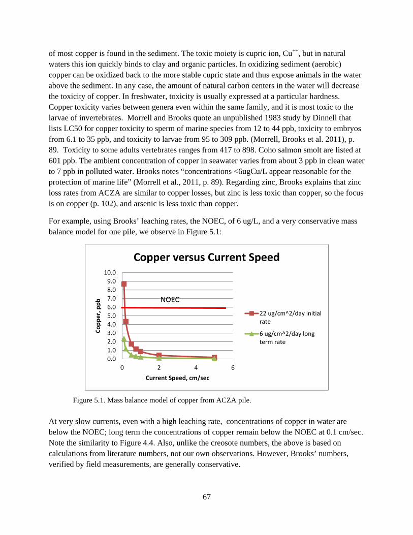
67

of most copper is found in the sediment. The toxic moiety is cupric ion, Cu++, but in natural waters this ion quickly binds to clay and organic particles. In oxidizing sediment (aerobic) copper can be oxidized back to the more stable cupric state and thus expose animals in the water above the sediment. In any case, the amount of natural carbon centers in the water will decrease the toxicity of copper. In freshwater, toxicity is usually expressed at a particular hardness. Copper toxicity varies between genera even within the same family, and it is most toxic to the larvae of invertebrates. Morrell and Brooks quote an unpublished 1983 study by Dinnell that lists LC50 for copper toxicity to sperm of marine species from 12 to 44 ppb, toxicity to embryos from 6.1 to 35 ppb, and toxicity to larvae from 95 to 309 ppb. (Morrell, Brooks et al. 2011), p. 89. Toxicity to some adults vertebrates ranges from 417 to 898. Coho salmon smolt are listed at 601 ppb. The ambient concentration of copper in seawater varies from about 3 ppb in clean water to 7 ppb in polluted water. Brooks notes “concentrations <6ugCu/L appear reasonable for the protection of marine life” (Morrell et al., 2011, p. 89). Regarding zinc, Brooks explains that zinc loss rates from ACZA are similar to copper losses, but zinc is less toxic than copper, so the focus is on copper (p. 102), and arsenic is less toxic than copper.

For example, using Brooks’ leaching rates, the NOEC, of 6 ug/L, and a very conservative mass balance model for one pile, we observe in Figure 5.1:

Figure 5.1. Mass balance model of copper from ACZA pile.

At very slow currents, even with a high leaching rate, concentrations of copper in water are below the NOEC; long term the concentrations of copper remain below the NOEC at 0.1 cm/sec. Note the similarity to Figure 4.4. Also, unlike the creosote numbers, the above is based on calculations from literature numbers, not our own observations. However, Brooks’ numbers, verified by field measurements, are generally conservative.

0.0

1.0

2.0

3.0

4.0

5.0

6.0

7.0

8.0

9.0

10.0

0 2 4 6

Copper, ppb

Current Speed, cm/sec

Copper versus Current Speed

22 ug/cm^2/day initialrate

6 ug/cm^2/day longterm rate

NOEC

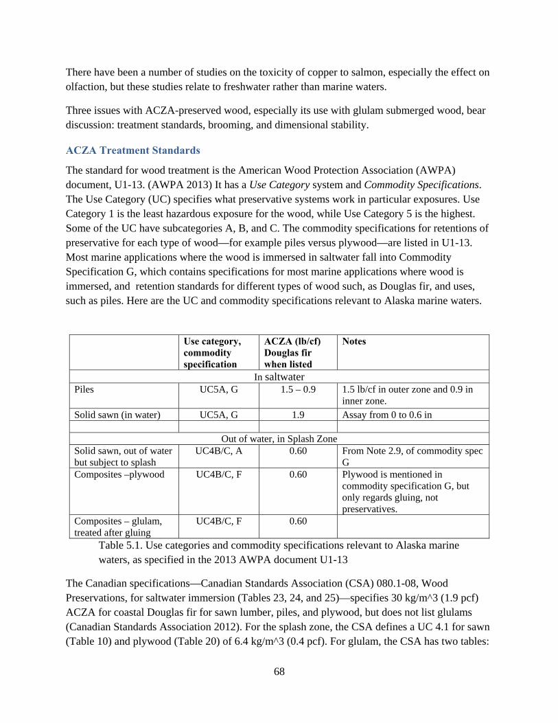
68

There have been a number of studies on the toxicity of copper to salmon, especially the effect on olfaction, but these studies relate to freshwater rather than marine waters.

Three issues with ACZA-preserved wood, especially its use with glulam submerged wood, bear discussion: treatment standards, brooming, and dimensional stability.

ACZA Treatment Standards

The standard for wood treatment is the American Wood Protection Association (AWPA) document, U1-13. (AWPA 2013) It has a Use Category system and Commodity Specifications. The Use Category (UC) specifies what preservative systems work in particular exposures. Use Category 1 is the least hazardous exposure for the wood, while Use Category 5 is the highest. Some of the UC have subcategories A, B, and C. The commodity specifications for retentions of preservative for each type of wood—for example piles versus plywood—are listed in U1-13. Most marine applications where the wood is immersed in saltwater fall into Commodity Specification G, which contains specifications for most marine applications where wood is immersed, and retention standards for different types of wood such, as Douglas fir, and uses, such as piles. Here are the UC and commodity specifications relevant to Alaska marine waters.

Use category, commodity specification

ACZA (lb/cf) Douglas fir when listed

Notes

In saltwater Piles UC5A, G 1.5 – 0.9 1.5 lb/cf in outer zone and 0.9 in

inner zone.

Solid sawn (in water) UC5A, G 1.9 Assay from 0 to 0.6 in

Out of water, in Splash Zone Solid sawn, out of water but subject to splash

UC4B/C, A 0.60 From Note 2.9, of commodity spec G

Composites –plywood UC4B/C, F 0.60 Plywood is mentioned in commodity specification G, but only regards gluing, not preservatives.

Composites – glulam, treated after gluing

UC4B/C, F 0.60

Table 5.1. Use categories and commodity specifications relevant to Alaska marine waters, as specified in the 2013 AWPA document U1-13

The Canadian specifications—Canadian Standards Association (CSA) 080.1-08, Wood Preservations, for saltwater immersion (Tables 23, 24, and 25)—specifies 30 kg/m^3 (1.9 pcf) ACZA for coastal Douglas fir for sawn lumber, piles, and plywood, but does not list glulams (Canadian Standards Association 2012). For the splash zone, the CSA defines a UC 4.1 for sawn (Table 10) and plywood (Table 20) of 6.4 kg/m^3 (0.4 pcf). For glulam, the CSA has two tables:

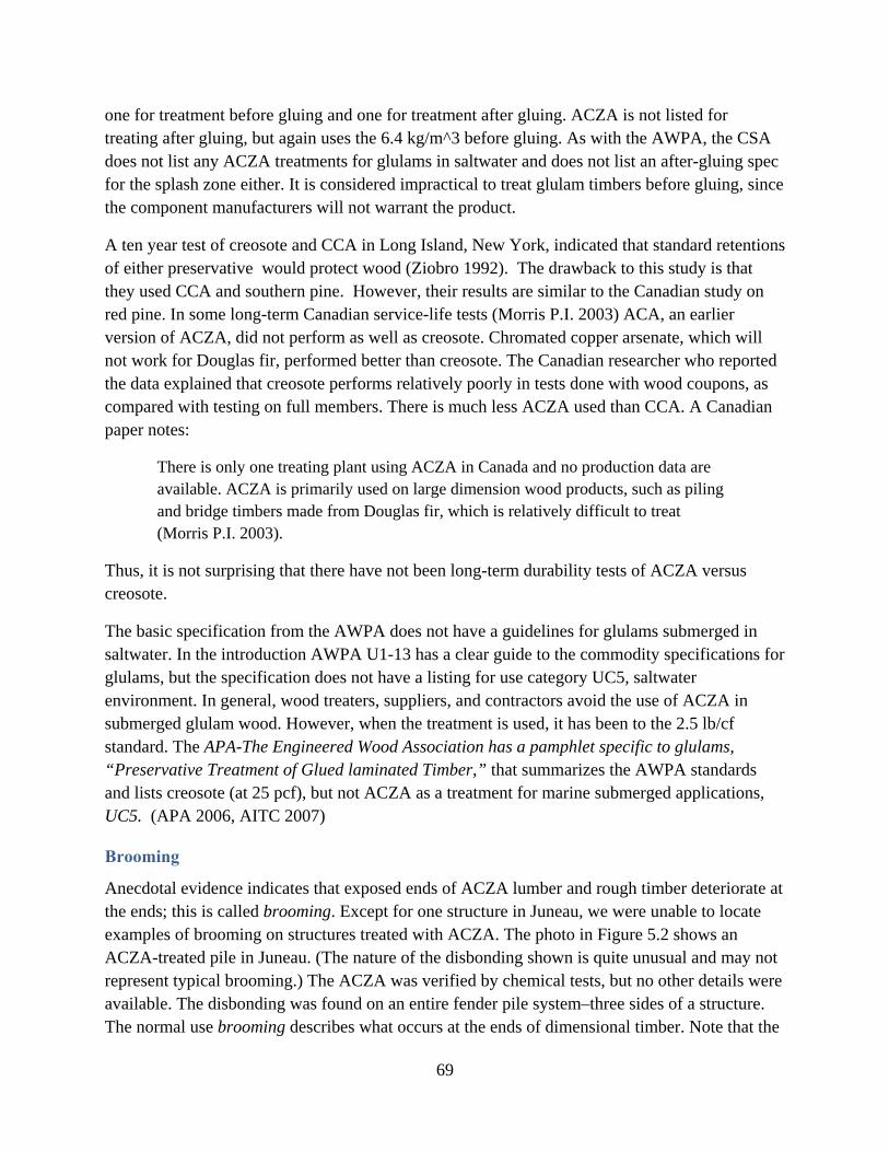
69

one for treatment before gluing and one for treatment after gluing. ACZA is not listed for treating after gluing, but again uses the 6.4 kg/m^3 before gluing. As with the AWPA, the CSA does not list any ACZA treatments for glulams in saltwater and does not list an after-gluing spec for the splash zone either. It is considered impractical to treat glulam timbers before gluing, since the component manufacturers will not warrant the product.

A ten year test of creosote and CCA in Long Island, New York, indicated that standard retentions of either preservative would protect wood (Ziobro 1992). The drawback to this study is that they used CCA and southern pine. However, their results are similar to the Canadian study on red pine. In some long-term Canadian service-life tests (Morris P.I. 2003) ACA, an earlier version of ACZA, did not perform as well as creosote. Chromated copper arsenate, which will not work for Douglas fir, performed better than creosote. The Canadian researcher who reported the data explained that creosote performs relatively poorly in tests done with wood coupons, as compared with testing on full members. There is much less ACZA used than CCA. A Canadian paper notes:

There is only one treating plant using ACZA in Canada and no production data are available. ACZA is primarily used on large dimension wood products, such as piling and bridge timbers made from Douglas fir, which is relatively difficult to treat (Morris P.I. 2003).

Thus, it is not surprising that there have not been long-term durability tests of ACZA versus creosote.

The basic specification from the AWPA does not have a guidelines for glulams submerged in saltwater. In the introduction AWPA U1-13 has a clear guide to the commodity specifications for glulams, but the specification does not have a listing for use category UC5, saltwater environment. In general, wood treaters, suppliers, and contractors avoid the use of ACZA in submerged glulam wood. However, when the treatment is used, it has been to the 2.5 lb/cf standard. The APA-The Engineered Wood Association has a pamphlet specific to glulams, “Preservative Treatment of Glued laminated Timber,” that summarizes the AWPA standards and lists creosote (at 25 pcf), but not ACZA as a treatment for marine submerged applications, UC5. (APA 2006, AITC 2007)

Brooming

Anecdotal evidence indicates that exposed ends of ACZA lumber and rough timber deteriorate at the ends; this is called brooming. Except for one structure in Juneau, we were unable to locate examples of brooming on structures treated with ACZA. The photo in Figure 5.2 shows an ACZA-treated pile in Juneau. (The nature of the disbonding shown is quite unusual and may not represent typical brooming.) The ACZA was verified by chemical tests, but no other details were available. The disbonding was found on an entire fender pile system–three sides of a structure. The normal use brooming describes what occurs at the ends of dimensional timber. Note that the

70

Juneau piles are in the dock’s fender pile system, had such deterioration occurred in bearing piles, the structure would be compromised and unsafe.

Figure 5.2. An ACZA-treated pile in Juneau, Alaska.

The American Institute of Timber Construction (AITC) has a specification—AITC 109–2007, Standard for Preservative Treatment of Structural Glued Laminated Timber, Table 2—allows ACZA use in water, but has a limitation note: “Wetting and redrying processes associated with treatment may result in dimensional changes, warping, checking, or splitting of members treated after gluing.” It is important to note that for Douglas fir, the AWPA only lists ACZA for use after gluing. In Section 4.2 of AITC 107-2007 it states that only Southern Pine is currently treated prior to gluing. Table 6 of the AITC’s specification does present a recommendation for UC5 of 2.5 lb/cf in a 0.6 inch assay zone, but that is only if treated before gluing. (AITC 2007). In a related FAQ pamphlet on , AITC acknowledges the occurrence of cracking and checking, but essentially recommends using treated glulams if appearance is not concern since these surface defects do not affect the structural strength (AITC 2008).

Thus, we have anecdotal observations of brooming, industry specifications, and literature that indicate surface defects—checking, raised grain, and shelling—are likely in ACZA-treated glulams. This cracking and checking could encourage marine borers, although we do not have reports of this being tested. Although it is possible that water-based ACZA will retain water and suffer freeze-thaw damage, another explanation is that documented surface defects and the lack of dimensional stability result in this apparent deterioration. It is also possible that some brooming is caused by the deposition and enlargement of salt crystals causing defibration.

71

Douglas fir pilings treated with ACZA develop more numerous and deeper checks compared with piling treated with oil-based copper naphthenate and presumably creosote. These checks increase the surface area available for leaching. One study indicates that the area increased 2.4 and 2.8-fold more than the neat circumference (Morrell, Brooks et al. 2011).

Sawn timber is often treated uncured. This practice reduces the surface defects indicated in glulams, which are kiln dried once or twice during the treatment process.

Dimensional Stability

Wood in marine structures may be divided into round pilings, sawn lumber, and composites (glulam and plywood). The water-based salts of ACZA absorb and lose water, which causes the wood to shrink and swell. This effect may be tolerable for piles and bull rails, but causes havoc

in dimensional lumber. One wood supplier reports that ACZA glulam deck panels, 3 1/8" 24" to 36", uniformly swelled over 1 1/4". The swelling was compensated for by pre-cutting the panels, but when the panels dried, they shrank and cracks opened between them.

Treating of glued laminated timber members with water-borne preservatives after gluing is not generally recommended. If glued laminated timbers are treated after gluing, dimensional changes caused by saturation of the wood with the water-borne preservatives and their carrier followed by subsequent re-drying may result in raised grain and excessive warping, checking, or splitting. The use of water-borne treated glued laminated timber members without adequate re-drying of the timbers prior to installation can also result in excessive deflections as well as checking, splitting and warping as previously mentioned as the members "season" in. (AITC 2008)

Hardware

ACZA causes corrosion in metal fasteners, which requires special precautions. Some specifications call for only stainless steel fasteners, while others suggest heavily galvanized.

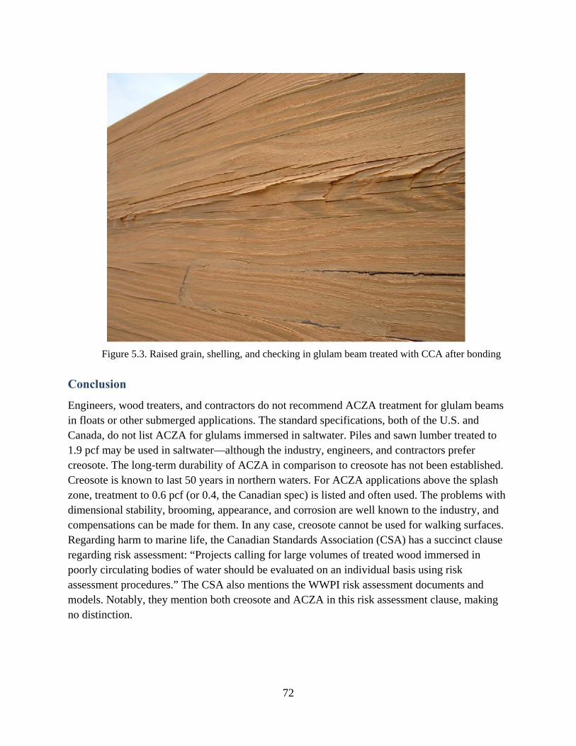
72

Figure 5.3. Raised grain, shelling, and checking in glulam beam treated with CCA after bonding

Conclusion

Engineers, wood treaters, and contractors do not recommend ACZA treatment for glulam beams in floats or other submerged applications. The standard specifications, both of the U.S. and Canada, do not list ACZA for glulams immersed in saltwater. Piles and sawn lumber treated to 1.9 pcf may be used in saltwater—although the industry, engineers, and contractors prefer creosote. The long-term durability of ACZA in comparison to creosote has not been established. Creosote is known to last 50 years in northern waters. For ACZA applications above the splash zone, treatment to 0.6 pcf (or 0.4, the Canadian spec) is listed and often used. The problems with dimensional stability, brooming, appearance, and corrosion are well known to the industry, and compensations can be made for them. In any case, creosote cannot be used for walking surfaces. Regarding harm to marine life, the Canadian Standards Association (CSA) has a succinct clause regarding risk assessment: “Projects calling for large volumes of treated wood immersed in poorly circulating bodies of water should be evaluated on an individual basis using risk assessment procedures.” The CSA also mentions the WWPI risk assessment documents and models. Notably, they mention both creosote and ACZA in this risk assessment clause, making no distinction.

73

Chapter 6. Risk Characterization

Risk characterization states the probability and severity of harm and discusses uncertainties. Since choices regarding wood preservatives in the marine environment must be made, we need to characterize the risks involved in the choices. For information on ACZA, we relied on literature, observations, and interviews. To obtain information on creosote, we relied on our laboratory work, which was guided by the literature. First, regarding the toxicity to herring eggs of wood preserved with creosote in the marine environment, we tried to establish the risks. The receptors are the eggs, but there are three exposure routes: the first is direct contact by the egg that was spawned onto the wood, the second is exposure of the egg very close to the pile, if the pile is fouled, and the third is exposure of the egg some distance away from pile, where the egg is attached to some other substrate.

In Chapter 2, we examined the COC chemicals in creosote.

In Chapter 3, we reviewed the toxicity of PAH from creosote wood to herring eggs and produced an NOEC and LC50.

In Chapter 4, we examined the likely concentrations of PAH from creosote derived from marine wood.

In Chapter 5, we reviewed ACZA.

In this Chapter 6, we will formulate the probability and severity or harm and close with some brief recommendations.

Discussion of Uncertainties

Next examine some of the uncertainties in our assessment, both general uncertainties as well as uncertainties that apply to particular situations. Since many of the creosote issues are not dissimilar to ACZA, we will review them as appropriate.

COC Chemicals

Creosote is defined by its coal of origin and its distillation temperatures and not by its chemical composition. Indeed, there are different compositions of commercial creosote. Appendix 2.1 has a compilation of studies that demonstrate the variance in composition. However, all the toxicity studies related to creosote assume that PAHs are the COC. This is because the other chemicals are assumed to be in small proportions to the PAH and like PAH are hydrophobic. It is likelty that small amounts of these, mostly hydrocarbon compounds, are in the leachate tested, but we do not believe these other chemicals would affect our conclusions. Likewise, sheen often occurs on water when new creosote is installed. The sheen, which is caused by lighter, volatile PAH, quickly oxidizes and is unlikely to harm pelagic species, certainly not herring eggs. The sheen quickly dissipates. We note that some authors only tested for parent PAH, but again, the

74

alkylated PAHs are generally a small portion of the PAH in creosote and the effects would remain proportional to the measured PAH.

We examined the chemicals in the leachate from end-sealed lumber where only cross grain leaching was possible, and leachate from lumber with end cuts where end-grain leaching was possible, and found some differences. These differences were not great enough to warrant treating PAH chemicals differently than TPAH.

Toxicity

Our study had substantial mortality in the controls and a large variation in effects for each treatment concentration. While high mortalities are common in egg experiments, ours exceeded the norm. Loading the slides past 150 eggs may have been a minor factor in the mortality, although the correlation was slight. There was a possibility of an infection in some of the beakers after the slides were removed from the aquaria. However, since we had a large number of slides per treatment, and nine treatments, and the slides were distributed randomly, the substantial amount of data can be used to inform judgment with some confidence. Our current NOEC, 4 ppb, is not different from work by others on herring eggs.

To some extent, we assume the effects of exposure to be additive; that is, the swimming disability and skeletal defects would add to the egg mortality for some net effect. On the other hand, the true zero-effect dose is higher than the NOEC. This would suggest that the LC50 (actually EC50) for these effects of about 25 ppb should be used in risk evaluations rather than the 100 ppb we suggest which corresponds to hatching success. However, since we base our recommendations on the NOEC, the LC50 does not affect our risk analysis.

Determining LC50 (or EC50) using Abbots procedure to account for control effects and then using Probit is the standard in the regulatory and risk assessment processes. But Probit requires at least two points with mortality above the controls and less than 100% in order to yield results with reasonable confidence bounds. Given the high control mortality and large variations, we needed to modify the standard procedure somewhat. Because we had six different ways of looking at the data: two set of data based on exposures, 16 or 21 females, and three sets based on egg loadings, 115, 150 or all eggs on a slide—we had six sets of results. None of these sets provided sufficient points to use Probit effectively. We also used a standard statistical method, ANOVA, and a novel method. We then applied our judgment to evaluate the results and did not attempt to place mathematical confidence limits on one data set, but provided the range of results. Our research student, who wrote the Appendix, used a different procedure whereby she eliminated all the slides with more than 100 eggs and then included the controls in a logistic analysis of the data. Using only one data set eliminates judgment. However, because the controls, with their high mortality, are not subtracted in the analysis, it cannot be used to determine the NOEL. However it does yield 95% confidence limits on the EC50. By this method, the confidence limits on the EC50 are 5 to 50 ppb.

75

Exposure

Our data indicates that water concentrations due to most creosote applications would be below the NOEC for a range of likely current velocities. We have confidence in this finding, but recognize several points of uncertainty:

1. Our data exclusively measured PAHs from creosote. If the harbor is already contaminated with PAH from other sources, this additional PAH burdens the environment. However, as noted in Chapter 1, if the waters are stagnant and the harbor is contaminated already, creosote could be excluded based on a risk assessment related to sediment criteria. ACZA would have the same issues.

2. The current meter we used was not certified for the slow currents we measured, but the results agreed with some visual observations and the experienced operator believes they were accurate. In any case, the results match similar current data.

3. We analyzed a lone pile then computed the additive of 10 piles in a row parallel to the current. For a matrix of 10-by-10 piles, the lateral dispersion from adjoining lines of piles would add. While this calculation can be done easily in an ideal situation, it is not a trivial calculation for a real harbor with varying depths and current speeds. The simple mass balance model indicates that the average concentration will be about the same as a simple mass balance model from one pile. However, this calculation does not tell how far from the installation that will happen.

For the LDPE analysis, the contact rate, Rs, in the ocean may be different from the rate used in our laboratory. Also, preliminary analysis indicates that not all PAH chemicals are equally absorbed by the LDPE.

Our analysis gives us some confidence in a general conclusion—if approximate currents are known and the harbor is not heavily polluted. If currents are slow, less than 0.2 cm/sec, the harbor is polluted, or there is low oxygen in the sediment, a more-detailed risk assessment is in order.

There are three putative exposure routes with varying levels of uncertainty associated with each one. The first exposure route is direct contact by the egg that was spawned onto the wood; the second exposure is of the egg very close to the pile, if the pile is fouled; and the third exposure is some distance away from pile, where the egg is attached to some other substrate. We did extensive analysis on this last exposure route. For the first two routes—direct spawning on a newly installed pile and spawn on fouling—we extrapolated from our research.

The second route involves herring spawning on fouling. The fouling of piles and marine wood is quite variable, as described in Wikipedia:

Biofouling is divided into microfouling — biofilm formation and bacterial adhesion — and macrofouling — attachment of larger organisms. Due to the distinct chemistry and

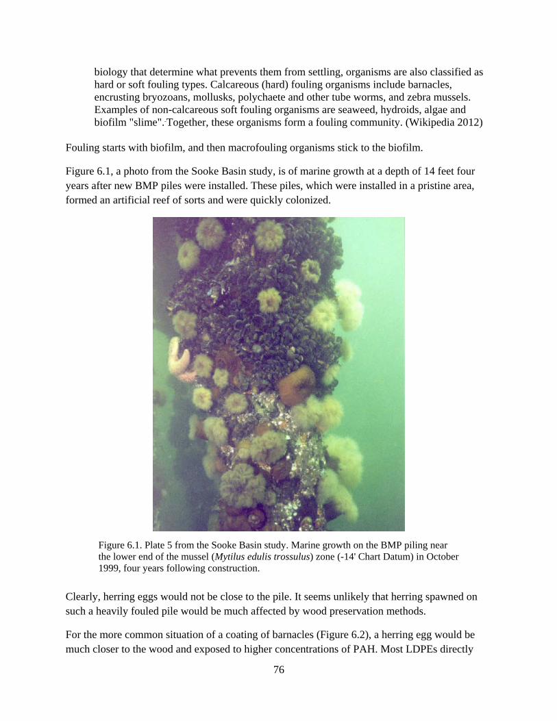
76

biology that determine what prevents them from settling, organisms are also classified as hard or soft fouling types. Calcareous (hard) fouling organisms include barnacles, encrusting bryozoans, mollusks, polychaete and other tube worms, and zebra mussels. Examples of non-calcareous soft fouling organisms are seaweed, hydroids, algae and biofilm "slime". Together, these organisms form a fouling community. (Wikipedia 2012)

Fouling starts with biofilm, and then macrofouling organisms stick to the biofilm.

Figure 6.1, a photo from the Sooke Basin study, is of marine growth at a depth of 14 feet four years after new BMP piles were installed. These piles, which were installed in a pristine area, formed an artificial reef of sorts and were quickly colonized.

Figure 6.1. Plate 5 from the Sooke Basin study. Marine growth on the BMP piling near the lower end of the mussel (Mytilus edulis trossulus) zone (-14' Chart Datum) in October 1999, four years following construction.

Clearly, herring eggs would not be close to the pile. It seems unlikely that herring spawned on such a heavily fouled pile would be much affected by wood preservation methods.

For the more common situation of a coating of barnacles (Figure 6.2), a herring egg would be much closer to the wood and exposed to higher concentrations of PAH. Most LDPEs directly

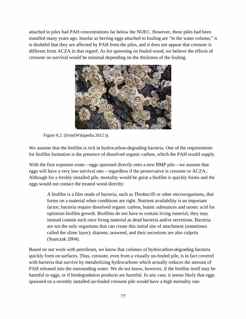
77

attached to piles had PAH concentrations far below the NOEC. However, these piles had been installed many years ago. Insofar as herring eggs attached to fouling are “in the water column,” it is doubtful that they are affected by PAH from the piles, and it does not appear that creosote is different from ACZA in that regard. As for spawning on fouled wood, we believe the effects of creosote on survival would be minimal depending on the thickness of the fouling.

Figure 6.2. (from(Wikipedia 2012 )).

We assume that the biofilm is rich in hydrocarbon-degrading bacteria. One of the requirements for biofilm formation is the presence of dissolved organic carbon, which the PAH would supply.

With the first exposure route—eggs spawned directly onto a new BMP pile—we assume that eggs will have a very low survival rate – regardless if the preservative is creosote or ACZA.. Although for a freshly installed pile, mortality would be great a biofilm is quickly forms and the eggs would not contact the treated wood directly:

A biofilm is a film made of bacteria, such as Thiobacilli or other microorganisms, that forms on a material when conditions are right. Nutrient availability is an important factor; bacteria require dissolved organic carbon, humic substances and uronic acid for optimum biofilm growth. Biofilms do not have to contain living material; they may instead contain such once living material as dead bacteria and/or secretions. Bacteria are not the only organisms that can create this initial site of attachment (sometimes called the slime layer); diatoms, seaweed, and their secretions are also culprits (Stanczak 2004).

Based on our work with petroleum, we know that colonies of hydrocarbon-degrading bacteria quickly form on surfaces. Thus, creosote, even from a visually un-fouled pile, is in fact covered with bacteria that survive by metabolizing hydrocarbons which actually reduces the amount of PAH released into the surrounding water. We do not know, however, if the biofilm itself may be harmful to eggs, or if biodegradation products are harmful. In any case, it seems likely that eggs spawned on a recently installed un-fouled creosote pile would have a high mortality rate.

78

Regarding ACZA, we do not have any evidence that un-fouled ACZA piles would be more hospitable to herring eggs. We speculate that the lack of carbon effluent from ACZA would retard biofilm growth relative to creosote, but ACZA piles are often fouled (Tarakanadha1 2004). A study in tropical waters indicated fouling by macroorganisms at the end of one month. Although the fouling of the ACZA test panel was less than the fouling of a CCA panel, all the water-based, mostly copper, preservatives fouled relatively quickly with macrofouling, indicating that biofilm formed quickly.

It seems likely that after a few weeks in the water, an un-fouled pile is in fact be covered by biofilm which would then serve as a barrier for the herring eggs from the pile.. Again, the biofilm itself may harm the eggs.

Regarding spawning directly onto a visibly un-fouled pile, which is probably fouled by biofilm, we believe the survival/hatching success would be impaired. We do not see any reason to prefer ACZA to creosote in this regard.

Risk Characterization and Recommendation

Exposure concentrations of herring eggs to PAH from newly installed BMP creosote-treated wood is below the NOEL of 4 ppb a short distance from the installation in typical Alaskan harbors. That critical distance varies with the average current and quantity of wood, but at an average current speed of 1 cm/sec, slower than typical Alaskan harbors, for a 100 pile installation, several meters from the outside pile would be a conservative estimate of that distance. Conceptually in the case of a new dock, the area under the dock itself and the nearby area stirred by ships’ props would not be suitable spawning habitat regardless of pile material —or in the case of wood piles, the preservative used. The region outside this zone would not be affected by PAH from the creosote-treated wood in the dock. A special risk assessment is required only if the installation is in waters with exceptionally low currents or water that is already polluted. We believe this evidence in the literature, our experiments and findings, and calculations based on those, support that characterization.

After several years, if the piles are fouled, the creosote is unlikely to affect eggs spawned on the fouling, based on the separation the fouling provides and our estimation of the biotransformation of PAH by the biofouling, as well as the decrease in leaching rates with time. We base this on our general estimation of the PAH concentrations in the water column close to the piles, which are considerably lower than the NOEC.

Herring eggs spawned directly on a new, unfouled pile, would be experience high mortality. Our calculations are not definite in the near field, very close to the pile, where lateral dispersion has not occurred. However, for newly installed piles, we do not see any difference between creosote and ACZA toxicity. For either, if herring stocks are stressed—and if they are likely to spawn on piles—construction should be delayed until after spawning season. Since the creosote leaching rates we measured in our lab decrease exponentially and were very low after 60 days, that likely

79

would provide a margin for construction before the spawning season, even in the absence of visible biofouling. However any biofouling would increase the factor of safety for the eggs.

80

Acknowledgements

First I thank my graduate student in Juneau, Danielle Duncan, who did the lion’s share of the work on the project and taught me some statistics on the side. Danielle was aided in Juneau by Mike Stekoll of UAS and Jeep Rice and Mark Carls of NOAA, who shared their vast experience with Danielle and I. Kenn Brooks and Jeff Morrell of OSU were very helpful throughout the project. J. R. Reynolds of Matheus and Jerry Farley of JH Baxter & Co. helped with materials and advice, as did Andrew Metzger of UAF and Dick Somerville of PND. Paul Morris of FPInnovations, the Canadian Forest Products research center, provided a helpful review and suggestions. Funding was provided by the Alaska Department of Transportation and Public Facilities and the Alaska University Transportation Center. Editing was provided by Fran Peterson, Anastasia Thayer, and Sandra Boatwright of UAF’s Institute of Northern Engineering.

81

References

AITC (2007). Standard for Preservative Treatment of Structural Glued Laminated Timber.

AITC (2008). Treating Glulam Timbers with Waterborne Preservatives; Answers to Commonly Asked Questions.

APA (2006). Preservative Treatment of Glued Laminated Timber.

AWPA (2010). Use Category System: User Specification for Treated Wood, American Wood Protection Association.

AWPA (2013). Use Category System: User Specification for Treated Wood, American Wood Protection Association

Boehm, P. D., G. S. Douglas, W. A. Burns, P. J. Mankiewicz, D. S. Page and A. E. Bence (1997). "Application of petroleum hydrocarbon chemical fingerprinting and allocation techniques after the Exxon Valdez oil spill." Marine Pollution Bulletin 34(8): 599-613.

Brooks, K. M. (2011). Chapter 7, Migration of Preservatives from Pressure Treated Wood. Managing Treated Wood in the Aquatic Enviroment. J. J. Morrell, K. M. Brooks and C. M. Davis, Forest Products Society.

Burns, W. A., P. J. Mankiewicz, A. E. Bence, D. S. Page and K. R. Parker (1997). "A principal-component and least-squares method for allocating polycyclic aromatic hydrocarbons in sediment to multiple sources." Environmental Toxicology and Chemistry 16(6): 1119-1131.

Canadian Standards Association (2012). 080 Series-08 Wood preservation.

Carls, M. G., L. Holland, M. Larsen, T. K. Collier, N. L. Scholz and J. P. Incardona (2008). "Fish embryos are damaged by dissolved PAHs, not oil particles." Aquatic Toxicology 88(2): 121-127.

Carls, M. G., L. G. Holland, J. W. Short, R. A. Heintz and S. D. Rice (2004). "Monitoring polynuclear aromatic hydrocarbons in aqueous environments with passive low-density polyethylene membrane devices." Environmental Toxicology and Chemistry 23(6): 1416-1424.

Carls, M. G., S. D. Rice and J. E. Hose (1999). "Sensitivity of fish embryos to weathered crude oil: Part I. Low-level exposure during incubation causes malformations, genetic damage, and mortality in larval pacific herring (Clupea pallasi)." Environmental Toxicology and Chemistry 18(3): 481-493.

Chapman, G. A., D.L. Denton, and J.M. Lazorchak (1995). Short-Term Methods for Estimating the Chronic Toxicity of Effluents and Receiving Waters to West Coast Marine and Estuarine Organisms EPA 600/R-95-136, EPA National Exposure Research Laboratory, U. S.Environmental Protection Agency, Cincinnati, OH

Christine Melber, J. K., and Inge Mangelsdorf (2004). Concise International Chemical Assessment Document 62: COAL TAR CREOSOTE. Geneva, Inter-Organization Programme for the Sound Management of Chemicals.

Clarke, J. U., Schroeder, P. R., and Steevens, J. A. (2002). Considerations for selection of Tier III water column toxicity standards for CDF effluent and runoff discharges: Statistical alternatives. Environmental Effects of Dredging Technical Notes Collection.

82

Elhassaneen, Y. A. (2004). "The effects of charcoal-broiled meat consumption on antioxidant defense system of erythrocytes and antioxidant vitamins in plasma." Nutrition Research 24(6): 435-446.

EPA (2002). Methods for Measuring the Acute Toxicity of Effluents and Receiving Waters to Freshwater and Marine Organisms.

EPA (2008). Reregistration Eligibility Decision for Creosote (Case 0139) EPA 739-R-08-007.

EPA (2008a). Updated Ecological Risk Assessment for Creosote

Fischer, H. B., E. J. List, r. C. Y. Koh, J. Imberger and N. H. Brooks (1979). Mixing in Inland and Coastal Waters. New York, Academic Press.

Goyette, D. and K. M. Brooks (1998). Creosote Evaluation: Phase II Sooke Basin Study - Baseline to 535 Days Post Construction 1995-1996.

Goyette, D. and K. M. Brooks (2001). ADDENDUM REPORT Continuation of the Sooke Basin Creosote Evaluation Study (Goyette and Brooks, 1998) Year Four – Day 1360 & Day 1540.

Huckins, J. N., J. D. Petty, J. A. Lebo, C. E. Orazio, R. C. Clark and V. L. Gibson (2012) "SPMD Technology Tutorial (3rd Edition)."

Ingram, L. L., G. D. McGinnis, L. Gjovik, R. and G. Roberson (1982). "Migration of Creosote and its Components from Treated Piling Sections in a Marine Environment." American Wood Preservers' Association: 120-128.

Kang, S.-M., J.J. Morrell, J. Simonsen and S. Lebow (2005). "Creosote Movement from Treated Wood Immersed in Fresh water." Forest Products Journal 55(12): 42-46.

Luellen, D. R. and D. Shea (2002). "Calibration and Field Verification of Semipermeable Membrane Devices for Measuring Polycyclic Aromatic Hydrocarbons in Water." Environmental Science & Technology 36(8): 1791-1797.

Morrell, J. J., K. M. Brooks and C. M. Davis, Eds. (2011). Managing Treated Wood in Aquatic Environments, Forest Products Society.

Morris P.I., I. J. K. (2003). "Field Testing of Wood Preservatives in Canada XII. Long Term Marine Tests." CWPA Proceedings 2003 238-255.

NOAA. (2008). "Juneau Harbor, North of: Station Info." Retrieved August 24, 2012, from http://tidesandcurrents.noaa.gov/cdata/StationList?type=Current Data&filter=survey&pid=21.

NOAA Fisheries - Southwest Region (2009). The use of treated wood products in aquatic environments. Guidelines to West Coast NOAA Fisheries Staff for Endangered Species Act and Essential Fish Habitat Consultations in the Alaska, Northwest and Southwest Regions.

Perkins, R. A. (2009). Creosote Treated Timber in the Alaskan Marine Environment.

Poston, T. (2001). Treated Wood Issues Associated with Overwater Structures in Marine and Freshwater Evniroments, Washington Department of Fish and Game, Washington Department of Ecology, Washington Department of Transportation.

Stanczak, M. (2004). "Biofouling: It's Not Just Barnacles Anymore

" Retrieved August 24, 2012, from http://www.csa.com/discoveryguides/biofoul/overview.php.

83

Stone, P. W. M. a. R. P. (2003). BENTHIC CURRENTS AT THREE NEARSHORE SITES NEAR POINT LENA AND AUKE BAY, ALASKA.

Sung-Mo, K., J. J. Morrell, J. Simonsen and S. Lebow (2005). "Creosote movement from treated wood immersed in fresh water." Forest Products Journal 55(12): 42-46.

Tarakanadha1, B., Jeffrey J. Morrell, and K. Satyanarayana Rao (2004). Impacts of Wood Preservatives (CCA, CCB, CDDC, ACZA, ACQ and

ACC) On the Settlement and Growth of Fouling Organisms. Environmental Impacts of Preservative-Treated Wood Conference. Orlando Florida USA.

Vines, C. A., T. Robbins, F. J. Griffin and G. N. Cherr (2000). "The effects of diffusible creosote-derived compounds on development in Pacific herring (Clupea pallasi)." Aquatic Toxicology 51(2): 225-239.

Wikipedia. (2012). "Biofouling." Retrieved 5 November, 2012, from http://en.wikipedia.org/wiki/Biofouling

Wikipedia. (2012 ). "Barnacle." Retrieved 5 November, 2012, from http://en.wikipedia.org/wiki/Barnacles

WWPI (2006). Western Wood Preservers Institute, Treated Wood Treated Wood in Aquatic Environments.

Xiao, Y. S., J.; Morrell, J.J. (2002). Effects of water flow rate and temperature on leaching from creosote-treated wood.: 6.

Ziobro, R., J. and Baileys, Randall, T. (1992). "Performance of Preservative Treated Wood Panels Exposed in Northerly Waters." Proceedings of the Eighty-Eighth Annual Meeting of the American Wood-Preservers' Association 88: 212-224.

84

APPENDIX LIST

The files listed as text are included in this Word or pdf document. The files noted as Excel are in separated Excel files transmitted with thie Word or pdf document.

Chapter 1

Text

1.0 Laboratory toxicity study of creosote-treated wood to Pacific herring (Clupea pallasii) embryos by D. Duncan, University of Alaska Fairbanks, School of Fisheries and Ocean Sciences

Chapter 2

Text

2.1 Chemicals in Creosote

2.2 List of PAH analytes for GC/MS analysis

2.3 PAH in wood

Excel

2.4 ACZA Leaching

Chapter 3

Excel: Chapter 3 Toxicity

Tabs:

3.1 All Toxicity Data. Has all the data from the all the observations, that is, it includes the eggs from females 1 to 21, and all the observations, hatching success, swimming ability, and deformations.

3.2 Full data in columns, 1-16. Has all the data from females 1-16, that is, females 17-21 data has been removed.

3.3 Sorted data, females 1-16, is the same as 3.2, but is now sorted by number of eggs per slide.

3.4 Females 1 to 16, 115 eggs, same as 3.3, but is filtered so only the data from slides with 115 or less eggs per slide are shown.

85

3.5 Females 1 to 16, 150 eggs, same as 3.3, but is filtered so only the data from slides with 150 or less eggs per slide are shown.

3.6 F[emales] 1 to 21, all slides, ANOVA. Mortality (hatching failure) all slides. Single factor ANOVA output tables on the right.

3.7 F[emales] 1 to 21, 150 eggs, ANOVA. Same as 3.6 but with only slides with 150 eggs or less.

3.8 F[emales] 1 to 21, 115 eggs, ANOVA. Same as 3.6 but with only slides with 115 eggs per slide or less.

3.9 F[emales] 1 to 16, all slides, ANOVA. Same as 3.6, but with only eggs from females 1 to 16. All slides regardless of egg loading.

3.10 F[emales] 1 to 16, 150 eggs, ANOVA. Same as 3.6, but with only eggs from females 1 to 16. Only slides with 150 or less eggs per slide.

3.11 F[emales] 1 to 16, 115 eggs, ANOVA. Same as 3.6, but with only eggs from females 1 to 16. Only slides with 115 or less eggs per slide..

3.12 Eggs per Slide vs mortality. Mortality of controls, both water and wood, sorted by number of eggs per slide and then three regression for all of the slides from those two sets, or only slides with 150 eggs or less or 115 eggs per slide.

3.13 All slides, females 1 -21. [Sorting workbook that arranged rows from first tab into columns. ]

3.14 Least Squares. Computations for least squares approach.

3.15 Abbotts. Worksheet with the computations for the Abbotts Formula analysis

3.16 Compute LC50. Worksheet with the computations for the LC 50 computations of egg mortality.

3.17 Skeletal Defects. Exposure concentrations and number with skeletal deformities are taken from earlier sheets and plotted.

3.18 Swimming Abnormally. Same as 3.17 but for abnormal swimming.

3.19 Graph of least squares with lowest value – best fit.

Chapter 4

Excel: Chapter 4 Exposure Evaluation: Leaching, fate and transport.

Tabs:

86

4.1 Pre-leaching. Initial leaching from pre-leach in garbage can and PVC tube and Treatment 7 in tox test which used boards that were not previously leached.

4.2 Leaching during tox tests. Using flow rate and GC data, this worksheet computes the leaching rates for the boards in the various treatments.

4.3 Water parameters. This has the water temperature, dissolved oxygen, pH and other parameters during the test.

4.4 Flow rates. Water flow rates for the pre-leaching and leaching during tox testing.

4.5 Sort Flow Rates. Organize flow rates and take average.

4.6 Wood dimensions. Calculate surface area for different combinations of wood.

4.7 Mass Balance for Report. This is the mass balance downstream concentration.

4.8 Fisher Calculations.

4.9 Field current data taken in Juneau near where LDPE were positioned.

4.10 Tide data during field current probes.

4.11 Current data from literature near LDPE locations by Juneau.

4.12 Current data from channel near LDPE locations.

4.13 Leaching from the literature calculations. Kang, Ingram, and Brooks data and calculations.

4.14 Turbulence. Calculation of Reynolds number and turbulence.

4.15 Leaching Graphic. Data for table of leaching rates from our lab and the literature.

4.16 Vines computations. Estimation of water concentrations based on our leaching rates and Vines wood chip size.

4.17 PAH vs time in treatments

4.18 GC data for all treatments. TPAH and PAH compounds from water extractions and grams of TPAH from LDPE sampler, rationalized to gram of sampler because larger sampler was put in after day 15, when eggs were removed.

4.19 Calculate Rs. This worksheet takes the mass of PAH in the LDPEs that were in our tox water and compares it to the average concentration of PAH in the water determined by

87

4.20 Burns least squares. This has a workup of LDPE PAH concentrations compared with PAH concentrations from sediments known to be contaminated with various sources of PAH.

4.21 Full chemistry. This worksheet has all the chemical analyses to 25 August 2012.

88

Appendix 1

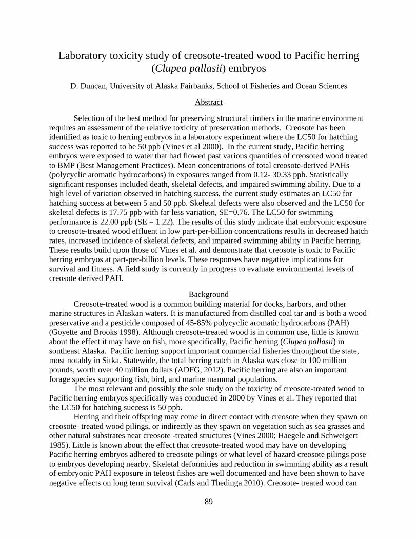
89

Laboratory toxicity study of creosote-treated wood to Pacific herring (Clupea pallasii) embryos

D. Duncan, University of Alaska Fairbanks, School of Fisheries and Ocean Sciences

Abstract

Selection of the best method for preserving structural timbers in the marine environment requires an assessment of the relative toxicity of preservation methods. Creosote has been identified as toxic to herring embryos in a laboratory experiment where the LC50 for hatching success was reported to be 50 ppb (Vines et al 2000). In the current study, Pacific herring embryos were exposed to water that had flowed past various quantities of creosoted wood treated to BMP (Best Management Practices). Mean concentrations of total creosote-derived PAHs (polycyclic aromatic hydrocarbons) in exposures ranged from 0.12- 30.33 ppb. Statistically significant responses included death, skeletal defects, and impaired swimming ability. Due to a high level of variation observed in hatching success, the current study estimates an LC50 for hatching success at between 5 and 50 ppb. Skeletal defects were also observed and the LC50 for skeletal defects is 17.75 ppb with far less variation, SE=0.76. The LC50 for swimming performance is 22.00 ppb (SE = 1.22). The results of this study indicate that embryonic exposure to creosote-treated wood effluent in low part-per-billion concentrations results in decreased hatch rates, increased incidence of skeletal defects, and impaired swimming ability in Pacific herring. These results build upon those of Vines et al. and demonstrate that creosote is toxic to Pacific herring embryos at part-per-billion levels. These responses have negative implications for survival and fitness. A field study is currently in progress to evaluate environmental levels of creosote derived PAH.

Background Creosote-treated wood is a common building material for docks, harbors, and other marine structures in Alaskan waters. It is manufactured from distilled coal tar and is both a wood preservative and a pesticide composed of 45-85% polycyclic aromatic hydrocarbons (PAH) (Goyette and Brooks 1998). Although creosote-treated wood is in common use, little is known about the effect it may have on fish, more specifically, Pacific herring (Clupea pallasii) in southeast Alaska. Pacific herring support important commercial fisheries throughout the state, most notably in Sitka. Statewide, the total herring catch in Alaska was close to 100 million pounds, worth over 40 million dollars (ADFG, 2012). Pacific herring are also an important forage species supporting fish, bird, and marine mammal populations. The most relevant and possibly the sole study on the toxicity of creosote-treated wood to Pacific herring embryos specifically was conducted in 2000 by Vines et al. They reported that the LC50 for hatching success is 50 ppb. Herring and their offspring may come in direct contact with creosote when they spawn on creosote- treated wood pilings, or indirectly as they spawn on vegetation such as sea grasses and other natural substrates near creosote -treated structures (Vines 2000; Haegele and Schweigert 1985). Little is known about the effect that creosote-treated wood may have on developing Pacific herring embryos adhered to creosote pilings or what level of hazard creosote pilings pose to embryos developing nearby. Skeletal deformities and reduction in swimming ability as a result of embryonic PAH exposure in teleost fishes are well documented and have been shown to have negative effects on long term survival (Carls and Thedinga 2010). Creosote- treated wood can

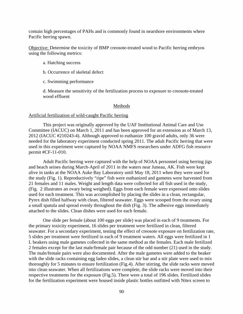
90

contain high percentages of PAHs and is commonly found in nearshore environments where Pacific herring spawn. Objective: Determine the toxicity of BMP creosote-treated wood to Pacific herring embryos using the following metrics:

a. Hatching success

b. Occurrence of skeletal defect

c. Swimming performance

d. Measure the sensitivity of the fertilization process to exposure to creosote-treated wood effluent

Methods

Artificial fertilization of wild-caught Pacific herring

This project was originally approved by the UAF Institutional Animal Care and Use Committee (IACUC) on March 1, 2011 and has been approved for an extension as of March 13, 2012 (IACUC #210243-4). Although approved to euthanize 100 gravid adults, only 36 were needed for the laboratory experiment conducted spring 2011. The adult Pacific herring that were used in this experiment were captured by NOAA NMFS researchers under ADFG fish resource permit #CF-11-010.

Adult Pacific herring were captured with the help of NOAA personnel using herring jigs and beach seines during March-April of 2011 in the waters near Juneau, AK. Fish were kept alive in tanks at the NOAA Auke Bay Laboratory until May 18, 2011 when they were used for the study (Fig. 1). Reproductively “ripe” fish were euthanized and gametes were harvested from 21 females and 11 males. Weight and length data were collected for all fish used in the study, (Fig. 2 illustrates an ovary being weighed). Eggs from each female were expressed onto slides used for each treatment. This was accomplished by placing the slides in a clean, rectangular, Pyrex dish filled halfway with clean, filtered seawater. Eggs were scooped from the ovary using a small spatula and spread evenly throughout the dish (Fig. 3). The adhesive eggs immediately attached to the slides. Clean dishes were used for each female.

One slide per female (about 100 eggs per slide) was placed in each of 9 treatments. For the primary toxicity experiment, 16 slides per treatment were fertilized in clean, filtered seawater. For a secondary experiment, testing the effect of creosote exposure on fertilization rate, 5 slides per treatment were fertilized in each of 9 treatment waters. All eggs were fertilized in 1 L beakers using male gametes collected in the same method as the females. Each male fertilized 2 females except for the last male/female pair because of the odd number (21) used in the study. The male/female pairs were also documented. After the male gametes were added to the beaker with the slide racks containing egg laden slides, a clean stir bar and a stir plate were used to mix thoroughly for 5 minutes to ensure fertilization (Fig.4). After stirring, the slide racks were moved into clean seawater. When all fertilizations were complete, the slide racks were moved into their respective treatments for the exposure (Fig.5). There were a total of 196 slides. Fertilized slides for the fertilization experiment were housed inside plastic bottles outfitted with Nitex screen to

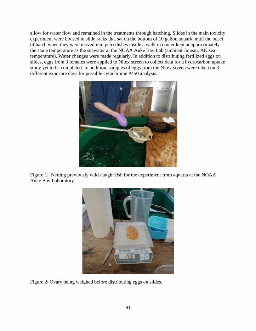
91

allow for water flow and remained in the treatments through hatching. Slides in the main toxicity experiment were housed in slide racks that sat on the bottom of 10 gallon aquaria until the onset of hatch when they were moved into petri dishes inside a walk in cooler kept at approximately the same temperature as the seawater at the NOAA Auke Bay Lab (ambient Juneau, AK sea temperature). Water changes were made regularly. In addition to distributing fertilized eggs on slides, eggs from 3 females were applied to Nitex screen to collect data for a hydrocarbon uptake study yet to be completed. In addition, samples of eggs from the Nitex screen were taken on 3 different exposure days for possible cytochrome P450 analysis.

Figure 1: Netting previously wild-caught fish for the experiment from aquaria at the NOAA Auke Bay Laboratory.

Figure 2: Ovary being weighed before distributing eggs on slides.

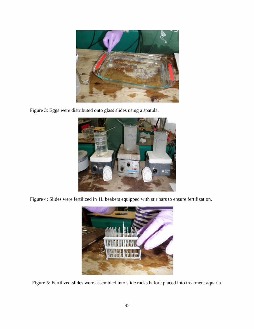
92

Figure 3: Eggs were distributed onto glass slides using a spatula.

Figure 4: Slides were fertilized in 1L beakers equipped with stir bars to ensure fertilization.

Figure 5: Fertilized slides were assembled into slide racks before placed into treatment aquaria.

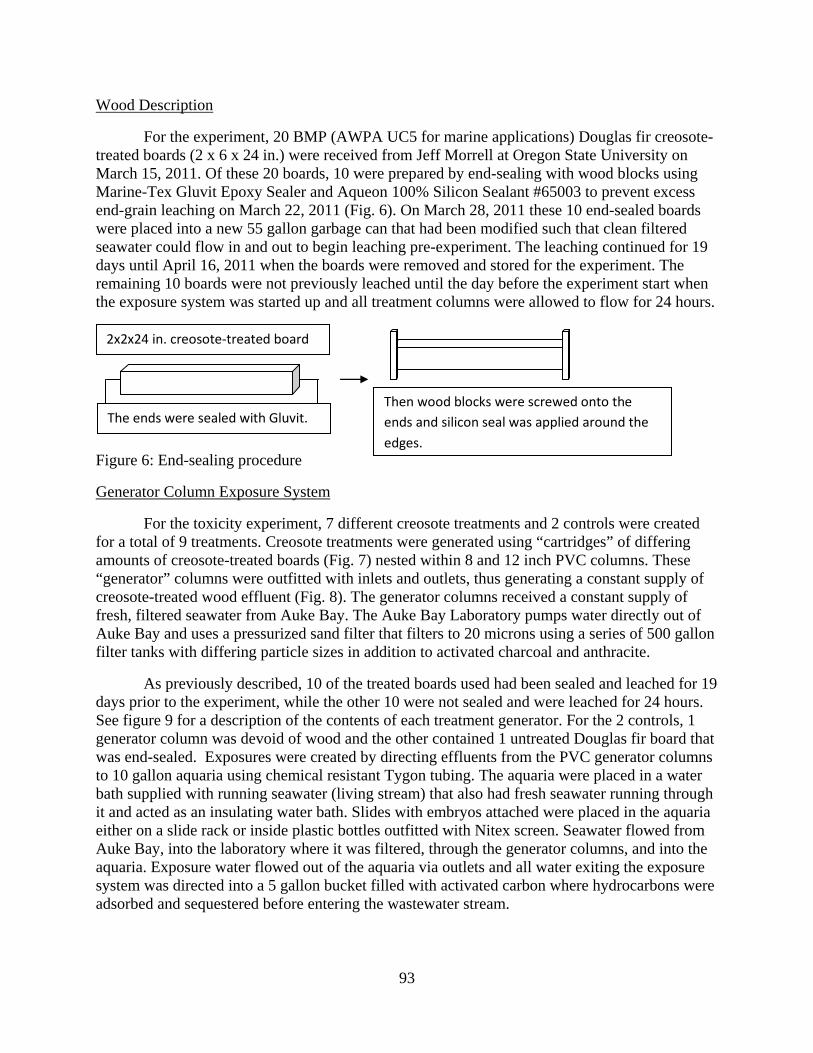
93

Wood Description

For the experiment, 20 BMP (AWPA UC5 for marine applications) Douglas fir creosote-treated boards (2 x 6 x 24 in.) were received from Jeff Morrell at Oregon State University on March 15, 2011. Of these 20 boards, 10 were prepared by end-sealing with wood blocks using Marine-Tex Gluvit Epoxy Sealer and Aqueon 100% Silicon Sealant #65003 to prevent excess end-grain leaching on March 22, 2011 (Fig. 6). On March 28, 2011 these 10 end-sealed boards were placed into a new 55 gallon garbage can that had been modified such that clean filtered seawater could flow in and out to begin leaching pre-experiment. The leaching continued for 19 days until April 16, 2011 when the boards were removed and stored for the experiment. The remaining 10 boards were not previously leached until the day before the experiment start when the exposure system was started up and all treatment columns were allowed to flow for 24 hours.

Figure 6: End-sealing procedure

Generator Column Exposure System

For the toxicity experiment, 7 different creosote treatments and 2 controls were created for a total of 9 treatments. Creosote treatments were generated using “cartridges” of differing amounts of creosote-treated boards (Fig. 7) nested within 8 and 12 inch PVC columns. These “generator” columns were outfitted with inlets and outlets, thus generating a constant supply of creosote-treated wood effluent (Fig. 8). The generator columns received a constant supply of fresh, filtered seawater from Auke Bay. The Auke Bay Laboratory pumps water directly out of Auke Bay and uses a pressurized sand filter that filters to 20 microns using a series of 500 gallon filter tanks with differing particle sizes in addition to activated charcoal and anthracite.

As previously described, 10 of the treated boards used had been sealed and leached for 19 days prior to the experiment, while the other 10 were not sealed and were leached for 24 hours. See figure 9 for a description of the contents of each treatment generator. For the 2 controls, 1 generator column was devoid of wood and the other contained 1 untreated Douglas fir board that was end-sealed. Exposures were created by directing effluents from the PVC generator columns to 10 gallon aquaria using chemical resistant Tygon tubing. The aquaria were placed in a water bath supplied with running seawater (living stream) that also had fresh seawater running through it and acted as an insulating water bath. Slides with embryos attached were placed in the aquaria either on a slide rack or inside plastic bottles outfitted with Nitex screen. Seawater flowed from Auke Bay, into the laboratory where it was filtered, through the generator columns, and into the aquaria. Exposure water flowed out of the aquaria via outlets and all water exiting the exposure system was directed into a 5 gallon bucket filled with activated carbon where hydrocarbons were adsorbed and sequestered before entering the wastewater stream.

  2x2x24 in. creosote‐treated board 

The ends were sealed with Gluvit. Then wood blocks were screwed onto the 

ends and silicon seal was applied around the 

edges.

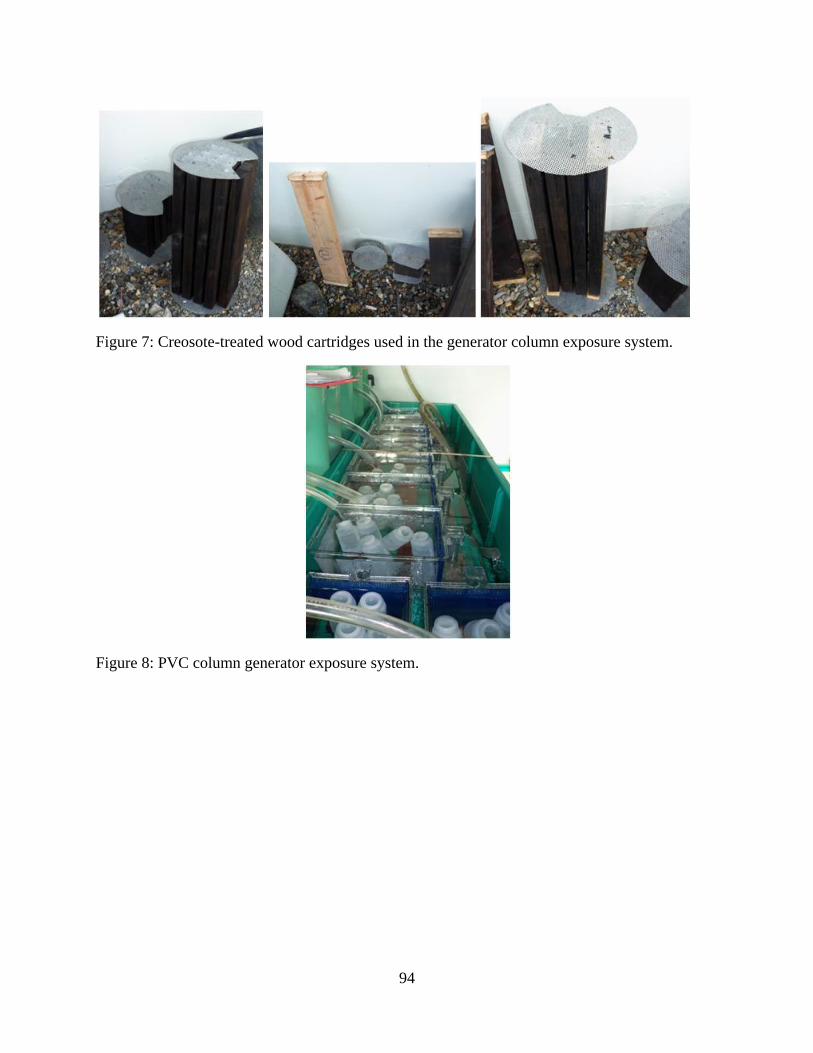
94

Figure 7: Creosote-treated wood cartridges used in the generator column exposure system.

Figure 8: PVC column generator exposure system.

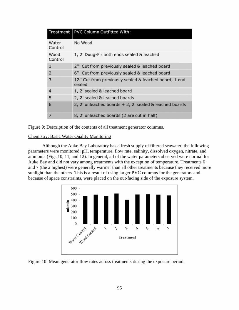
Figure 9:

Chemistr

AparameteammoniaAuke Baand 7 (thsunlight tbecause o

Figure 10

: Description

ry: Basic Wa

Although the ers were mona (Figs.10, 1y and did no

he 2 highest) than the otheof space con

0: Mean gen

n of the cont

ater Quality

Auke Bay Lnitored: pH, 1, and 12). I

ot vary amonwere genera

ers. This is anstraints, wer

nerator flow r

tents of all tr

Monitoring

Laboratory htemperature

In general, alng treatmentally warmer a result of usre placed on

rates across

95

reatment gen

has a fresh sue, flow rate, sll of the wats with the exthan all othe

sing larger Pn the out-faci

treatments d

nerator colum

upply of filtesalinity, disser parameterxception of ter treatments

PVC columnsing side of th

during the ex

mns.

ered seawatesolved oxygers observed temperature.s because ths for the genhe exposure

xposure peri

er, the followen, nitrate, awere norma. Treatmentsey received

nerators and system.

od.

wing and l for

s 6 more

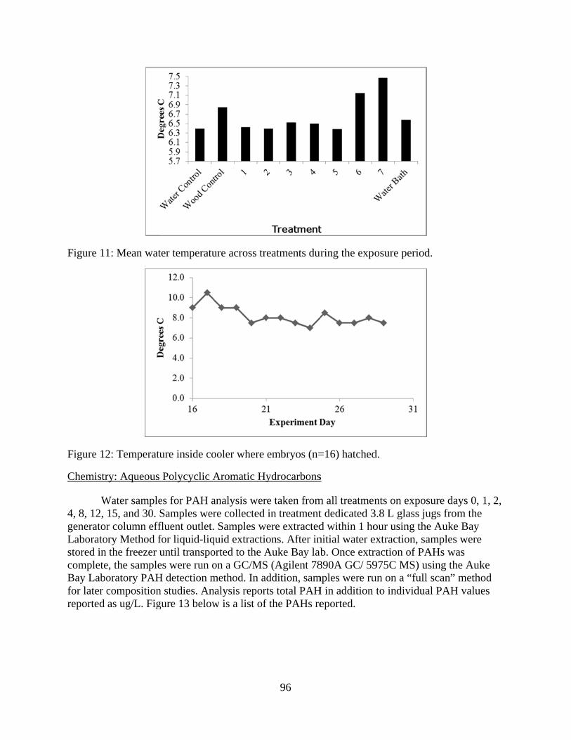
Figure 11

Figure 12

Chemistr

W4, 8, 12, generatorLaboratostored in completeBay Labofor later creported

1: Mean wat

2: Temperatu

ry: Aqueous

Water sample15, and 30. Sr column eff

ory Method fthe freezer u

e, the sampleoratory PAHcompositionas ug/L. Fig

ter temperatu

ure inside co

Polycyclic A

es for PAH aSamples werfluent outlet.for liquid-liquntil transpoes were run oH detection mn studies. Angure 13 below

ure across tre

ooler where

Aromatic Hy

analysis werere collected . Samples wequid extractioorted to the Aon a GC/MSmethod. In adnalysis reportw is a list of

96

eatments dur

embryos (n=

ydrocarbons

e taken fromin treatmentere extractedons. After inAuke Bay labS (Agilent 78ddition, samts total PAH

f the PAHs re

ring the exp

=16) hatched

s

m all treatmet dedicated 3d within 1 honitial water eb. Once extr

890A GC/ 59mples were ruH in addition eported.

osure period

d.

nts on expos3.8 L glass juour using theextraction, saraction of PA975C MS) uun on a “fullto individua

d.

sure days 0, ugs from thee Auke Bay amples wereAHs was using the Auk scan” methal PAH valu

1, 2, e

e

ke od es

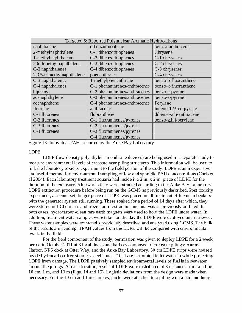
97

Targeted & Reported Polynuclear Aromatic Hydrocarbons naphthalene dibenzothiophene benz-a-anthracene 2-methylnaphthalene C-1 dibenzothiophenes Chrysene 1-methylnaphthalene C-2 dibenzothiophenes C-1 chrysenes 2,6-dimethylnaphthalene C-3 dibenzothiophenes C-2 chrysenes C-2 naphthalenes C-4 dibenzothiophenes C-3 chrysenes 2,3,5-trimethylnaphthalene phenanthrene C-4 chrysenes C-3 naphthalenes 1-methylphenanthrene benzo-b-fluoranthene C-4 naphthalenes C-1 phenanthrenes/anthracenes benzo-k-fluoranthene biphenyl C-2 phenanthrenes/anthracenes benzo-e-pyrene acenaphthylene C-3 phenanthrenes/anthracenes benzo-a-pyrene acenaphthene C-4 phenanthrenes/anthracenes Perylene fluorene anthracene indeno-123-cd-pyrene C-1 fluorenes fluoranthene dibenzo-a,h-anthracene C-2 fluorenes C-1 fluoranthenes/pyrenes benzo-g,h,i-perylene C-3 fluorenes C-2 fluoranthenes/pyrenes C-4 fluorenes C-3 fluoranthenes/pyrenes C-4 fluoranthenes/pyrenes

Figure 13: Individual PAHs reported by the Auke Bay Laboratory.

LDPE LDPE (low-density polyethylene membrane devices) are being used in a separate study to measure environmental levels of creosote near piling structures. This information will be used to link the laboratory toxicity experiment to the field portion of the study. LDPE is an inexpensive and useful method for environmental sampling of low and sporadic PAH concentrations (Carls et al 2004). Each laboratory treatment aquaria had inside it a 2 in. x 2 in. piece of LDPE for the duration of the exposure. Afterwards they were extracted according to the Auke Bay Laboratory LDPE extraction procedure before being run on the GCMS as previously described. Post toxicity experiment, a second set, longer piece of LDPE was placed in all treatment effluents in beakers with the generator system still running. These soaked for a period of 14 days after which, they were stored in I-Chem jars and frozen until extraction and analysis as previously outlined. In both cases, hydrocarbon-clean rare earth magnets were used to hold the LDPE under water. In addition, treatment water samples were taken on the day the LDPE were deployed and retrieved. These water samples were extracted s previously described and analyzed using GCMS. The bulk of the results are pending. TPAH values from the LDPE will be compared with environmental levels in the field. For the field component of the study, permission was given to deploy LDPE for a 2 week period in October 2011 at 3 local docks and harbors composed of creosote pilings: Aurora Harbor, NPS dock at Otter Way, and the Auke Bay Laboratory. 50 cm LDPE strips were housed inside hydrocarbon-free stainless steel “pucks” that are perforated to let water in while protecting LDPE from damage. The LDPE passively sampled environmental levels of PAHs in seawater around the pilings. At each location, 5 sets of LDPE were distributed at 3 distances from a piling: 10 cm, 1 m, and 10 m (Figs. 14 and 15). Logistic deviations from the design were made when necessary. For the 10 cm and 1 m samples, pucks were attached to a piling with a nail and hung

98

approximately arm’s length below the water line using nylon rope or they were hung along a rope between pilings. The 10 m samples were devised by using buoys and anchors to keep the pucks in position and under water (Fig. 16). The pucks were retrieved, double-wrapped in aluminum foil, and bagged separately before being frozen until they were extracted. Lab and field blanks were also utilized to verify that no PAH contamination had occurred. In addition, 3 water samples (low tide, mid tide, high tide) were taken at each dock/harbor at 10 cm from a piling where a LDPE sampler was deployed. These water samples were taken and extracted as previously described and the bulk of the results are pending. At each location, a sample of creosote from a piling was also taken and may be analyzed at a later date. We also placed a couple pucks in the air at Auke Bay Laboratory and put a couple halfway submerged in water.

Figure 14: 10 cm and 1 m LDPE distributed within a “matrix” of pilings at Auke Bay Laboratory.

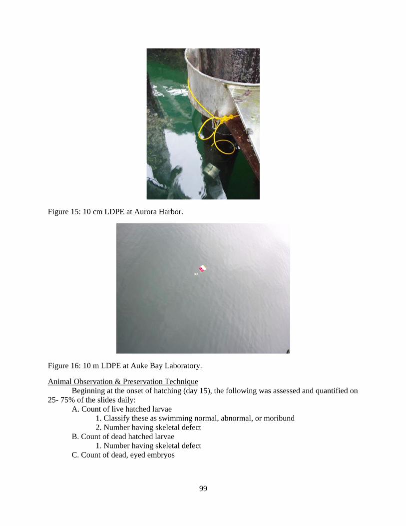
99

Figure 15: 10 cm LDPE at Aurora Harbor.

Figure 16: 10 m LDPE at Auke Bay Laboratory.

Animal Observation & Preservation Technique Beginning at the onset of hatching (day 15), the following was assessed and quantified on 25- 75% of the slides daily: A. Count of live hatched larvae 1. Classify these as swimming normal, abnormal, or moribund 2. Number having skeletal defect B. Count of dead hatched larvae 1. Number having skeletal defect C. Count of dead, eyed embryos

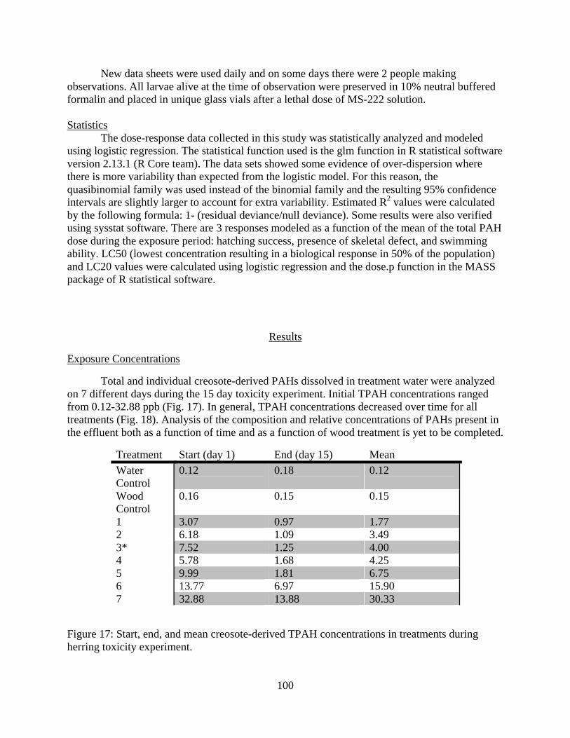
100

New data sheets were used daily and on some days there were 2 people making observations. All larvae alive at the time of observation were preserved in 10% neutral buffered formalin and placed in unique glass vials after a lethal dose of MS-222 solution. Statistics The dose-response data collected in this study was statistically analyzed and modeled using logistic regression. The statistical function used is the glm function in R statistical software version 2.13.1 (R Core team). The data sets showed some evidence of over-dispersion where there is more variability than expected from the logistic model. For this reason, the quasibinomial family was used instead of the binomial family and the resulting 95% confidence intervals are slightly larger to account for extra variability. Estimated R2 values were calculated by the following formula: 1- (residual deviance/null deviance). Some results were also verified using sysstat software. There are 3 responses modeled as a function of the mean of the total PAH dose during the exposure period: hatching success, presence of skeletal defect, and swimming ability. LC50 (lowest concentration resulting in a biological response in 50% of the population) and LC20 values were calculated using logistic regression and the dose.p function in the MASS package of R statistical software.

Results

Exposure Concentrations

Total and individual creosote-derived PAHs dissolved in treatment water were analyzed on 7 different days during the 15 day toxicity experiment. Initial TPAH concentrations ranged from 0.12-32.88 ppb (Fig. 17). In general, TPAH concentrations decreased over time for all treatments (Fig. 18). Analysis of the composition and relative concentrations of PAHs present in the effluent both as a function of time and as a function of wood treatment is yet to be completed.

Treatment Start (day 1) End (day 15) Mean

Water Control

0.12 0.18 0.12

Wood Control

0.16 0.15 0.15

1 3.07 0.97 1.77 2 6.18 1.09 3.49 3* 7.52 1.25 4.00 4 5.78 1.68 4.25 5 9.99 1.81 6.75 6 13.77 6.97 15.90 7 32.88 13.88 30.33

Figure 17: Start, end, and mean creosote-derived TPAH concentrations in treatments during herring toxicity experiment.

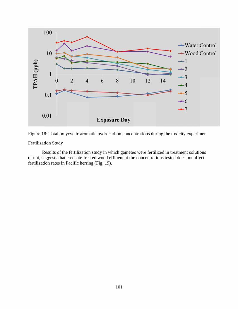
Figure 18

Fertilizat

Ror not, sufertilizati

8: Total poly

tion Study

Results of theuggests that cion rates in P

ycyclic arom

e fertilizationcreosote-treaPacific herrin

matic hydroca

n study in whated wood efng (Fig. 19).

101

arbon concen

hich gameteffluent at the.

ntrations dur

es were fertile concentrat

ring the toxi

lized in treattions tested d

icity experim

tment solutiodoes not affe

ment

ons ect

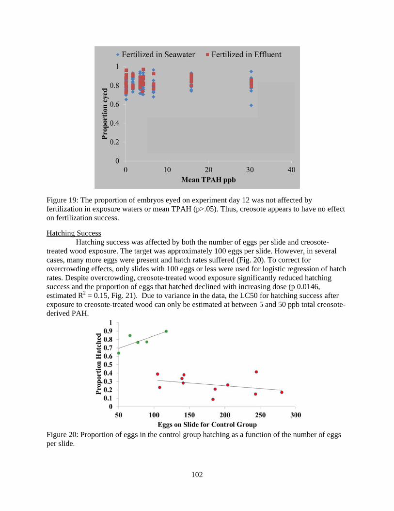
Figure 19fertilization fertiliz

Hatching treated wcases, maovercrowrates. Desuccess aestimatedexposurederived P

Figure 20per slide.

9: The propoion in exposuzation succe

g Success Hatching su

wood exposurany more eg

wding effectsspite overcro

and the propod R2 = 0.15, e to creosote-PAH.

0: Proportion.

ortion of embure waters o

ess.

uccess was are. The targe

ggs were press, only slidesowding, creoortion of eggFig. 21). Du-treated woo

n of eggs in

bryos eyed oor mean TPA

affected by bet was approsent and hatcs with 100 egosote-treatedgs that hatchue to varianc

od can only b

the control g

102

on experimenAH (p>.05). T

both the numoximately 10ch rates suffggs or less wd wood expohed declined ce in the datbe estimated

group hatchi

nt day 12 waThus, creoso

mber of eggs 00 eggs per sfered (Fig. 20were used forosure signific

with increasta, the LC50 d at between

ing as a func

as not affectote appears t

per slide anslide. Howev0). To correcr logistic regcantly reducsing dose (pfor hatching5 and 50 pp

ction of the n

ted by to have no ef

d creosote-ver, in severact for gression of hced hatching 0.0146, g success aftpb total creos

number of eg

ffect

al

hatch

ter sote-

ggs

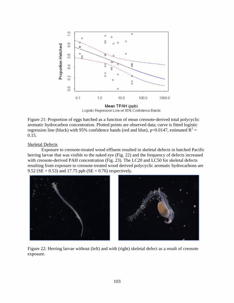
103

Figure 21: Proportion of eggs hatched as a function of mean creosote-derived total polycyclic aromatic hydrocarbon concentration. Plotted points are observed data; curve is fitted logistic regression line (black) with 95% confidence bands (red and blue), p=0.0147, estimated R2 = 0.15.

Skeletal Defects Exposure to creosote-treated wood effluent resulted in skeletal defects in hatched Pacific herring larvae that was visible to the naked eye (Fig. 22) and the frequency of defects increased with creosote-derived PAH concentration (Fig. 23). The LC20 and LC50 for skeletal defects resulting from exposure to creosote-treated wood derived polycyclic aromatic hydrocarbons are 9.52 (SE = 0.53) and 17.75 ppb (SE = 0.76) respectively.

Figure 22: Herring larvae without (left) and with (right) skeletal defect as a result of creosote exposure.

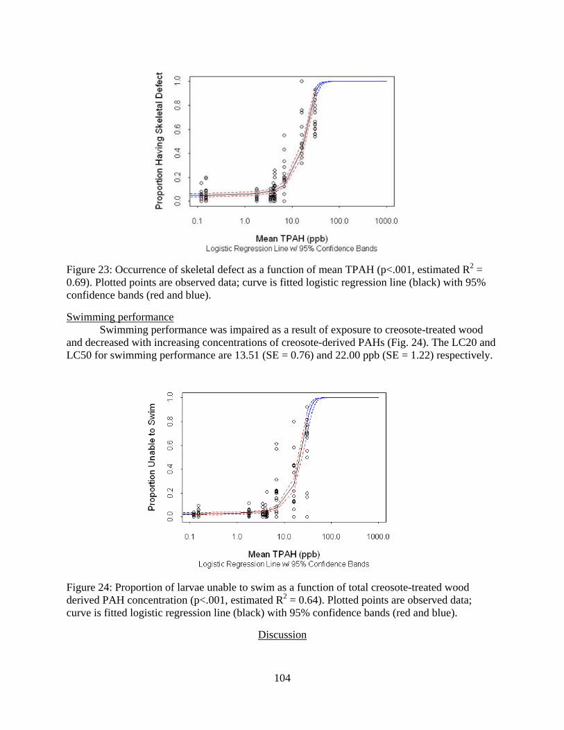
104

Figure 23: Occurrence of skeletal defect as a function of mean TPAH (p<.001, estimated R2 = 0.69). Plotted points are observed data; curve is fitted logistic regression line (black) with 95% confidence bands (red and blue).

Swimming performance Swimming performance was impaired as a result of exposure to creosote-treated wood and decreased with increasing concentrations of creosote-derived PAHs (Fig. 24). The LC20 and LC50 for swimming performance are 13.51 (SE = 0.76) and 22.00 ppb (SE = 1.22) respectively.

Figure 24: Proportion of larvae unable to swim as a function of total creosote-treated wood derived PAH concentration (p<.001, estimated R2 = 0.64). Plotted points are observed data; curve is fitted logistic regression line (black) with 95% confidence bands (red and blue).

Discussion

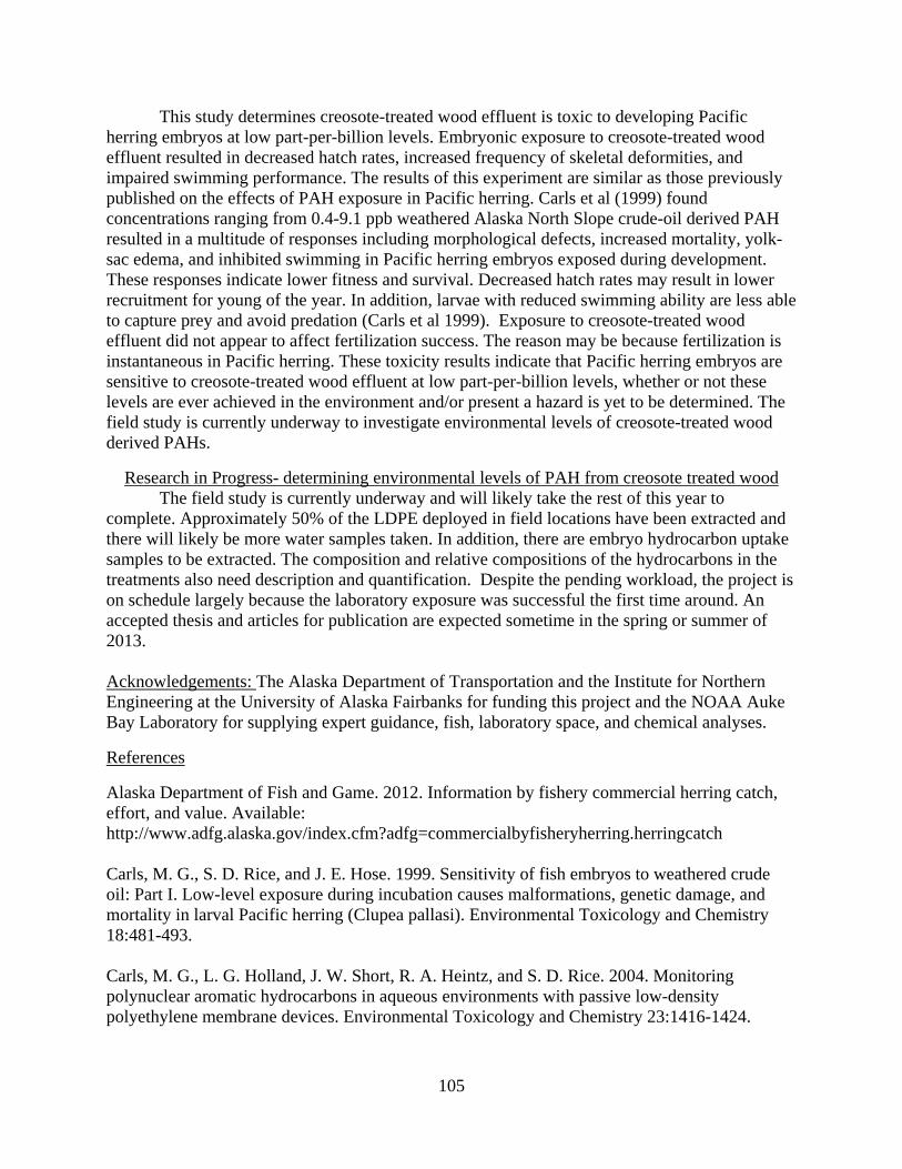
105

This study determines creosote-treated wood effluent is toxic to developing Pacific herring embryos at low part-per-billion levels. Embryonic exposure to creosote-treated wood effluent resulted in decreased hatch rates, increased frequency of skeletal deformities, and impaired swimming performance. The results of this experiment are similar as those previously published on the effects of PAH exposure in Pacific herring. Carls et al (1999) found concentrations ranging from 0.4-9.1 ppb weathered Alaska North Slope crude-oil derived PAH resulted in a multitude of responses including morphological defects, increased mortality, yolk-sac edema, and inhibited swimming in Pacific herring embryos exposed during development. These responses indicate lower fitness and survival. Decreased hatch rates may result in lower recruitment for young of the year. In addition, larvae with reduced swimming ability are less able to capture prey and avoid predation (Carls et al 1999). Exposure to creosote-treated wood effluent did not appear to affect fertilization success. The reason may be because fertilization is instantaneous in Pacific herring. These toxicity results indicate that Pacific herring embryos are sensitive to creosote-treated wood effluent at low part-per-billion levels, whether or not these levels are ever achieved in the environment and/or present a hazard is yet to be determined. The field study is currently underway to investigate environmental levels of creosote-treated wood derived PAHs.

Research in Progress- determining environmental levels of PAH from creosote treated wood The field study is currently underway and will likely take the rest of this year to complete. Approximately 50% of the LDPE deployed in field locations have been extracted and there will likely be more water samples taken. In addition, there are embryo hydrocarbon uptake samples to be extracted. The composition and relative compositions of the hydrocarbons in the treatments also need description and quantification. Despite the pending workload, the project is on schedule largely because the laboratory exposure was successful the first time around. An accepted thesis and articles for publication are expected sometime in the spring or summer of 2013. Acknowledgements: The Alaska Department of Transportation and the Institute for Northern Engineering at the University of Alaska Fairbanks for funding this project and the NOAA Auke Bay Laboratory for supplying expert guidance, fish, laboratory space, and chemical analyses.

References

Alaska Department of Fish and Game. 2012. Information by fishery commercial herring catch, effort, and value. Available: http://www.adfg.alaska.gov/index.cfm?adfg=commercialbyfisheryherring.herringcatch Carls, M. G., S. D. Rice, and J. E. Hose. 1999. Sensitivity of fish embryos to weathered crude oil: Part I. Low-level exposure during incubation causes malformations, genetic damage, and mortality in larval Pacific herring (Clupea pallasi). Environmental Toxicology and Chemistry 18:481-493. Carls, M. G., L. G. Holland, J. W. Short, R. A. Heintz, and S. D. Rice. 2004. Monitoring polynuclear aromatic hydrocarbons in aqueous environments with passive low-density polyethylene membrane devices. Environmental Toxicology and Chemistry 23:1416-1424.

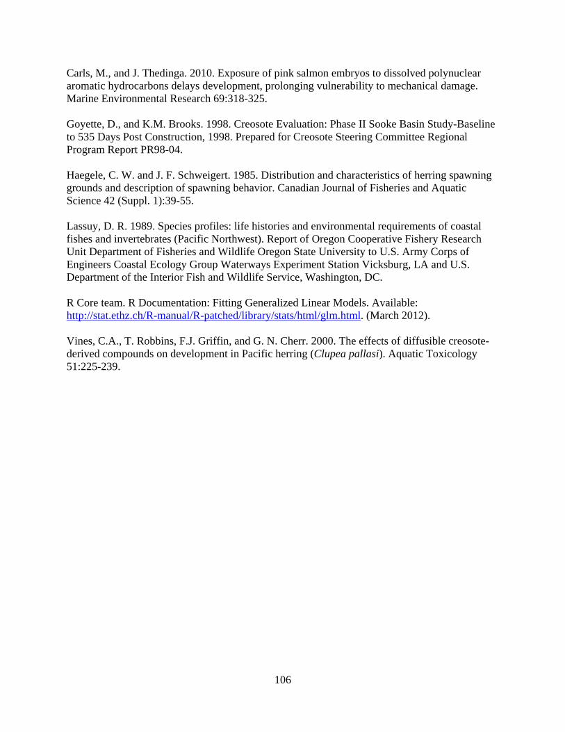
106

Carls, M., and J. Thedinga. 2010. Exposure of pink salmon embryos to dissolved polynuclear aromatic hydrocarbons delays development, prolonging vulnerability to mechanical damage. Marine Environmental Research 69:318-325. Goyette, D., and K.M. Brooks. 1998. Creosote Evaluation: Phase II Sooke Basin Study-Baseline to 535 Days Post Construction, 1998. Prepared for Creosote Steering Committee Regional Program Report PR98-04. Haegele, C. W. and J. F. Schweigert. 1985. Distribution and characteristics of herring spawning grounds and description of spawning behavior. Canadian Journal of Fisheries and Aquatic Science 42 (Suppl. 1):39-55. Lassuy, D. R. 1989. Species profiles: life histories and environmental requirements of coastal fishes and invertebrates (Pacific Northwest). Report of Oregon Cooperative Fishery Research Unit Department of Fisheries and Wildlife Oregon State University to U.S. Army Corps of Engineers Coastal Ecology Group Waterways Experiment Station Vicksburg, LA and U.S. Department of the Interior Fish and Wildlife Service, Washington, DC. R Core team. R Documentation: Fitting Generalized Linear Models. Available: http://stat.ethz.ch/R-manual/R-patched/library/stats/html/glm.html. (March 2012). Vines, C.A., T. Robbins, F.J. Griffin, and G. N. Cherr. 2000. The effects of diffusible creosote-derived compounds on development in Pacific herring (Clupea pallasi). Aquatic Toxicology 51:225-239.

107

Appendix 2

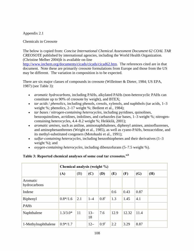
108

Appendix 2.1

Chemicals in Creosote

The below is copied from: Concise International Chemical Assessment Document 62 COAL TAR CREOSOTE published by international agencies, including the World Health Organization. (Christine Melber 2004)It is available on-line http://www.inchem.org/documents/cicads/cicads/cicad62.htm. The references cited are in that document. Note these are primarily creosote formulations from Europe and those from the US may be different. The variation in composition is to be expected.

There are six major classes of compounds in creosote (Willeitner & Dieter, 1984; US EPA, 1987) (see Table 3):

aromatic hydrocarbons, including PAHs, alkylated PAHs (non-heterocyclic PAHs can constitute up to 90% of creosote by weight), and BTEX;

tar acids / phenolics, including phenols, cresols, xylenols, and naphthols (tar acids, 1–3 weight %; phenolics, 2–17 weight %; Bedient et al., 1984);

tar bases / nitrogen-containing heterocycles, including pyridines, quinolines, benzoquinolines, acridines, indolines, and carbazoles (tar bases, 1–3 weight %; nitrogen-containing heterocycles, 4.4–8.2 weight %; Heikkilä, 2001);

aromatic amines, such as aniline, aminonaphthalenes, diphenyl amines, aminofluorenes, and aminophenanthrenes (Wright et al., 1985), as well as cyano-PAHs, benzacridine, and its methyl-substituted congeners (Motohashi et al., 1991);

sulfur-containing heterocycles, including benzothiophenes and their derivatives (1–3 weight %); and

oxygen-containing heterocycles, including dibenzofurans (5–7.5 weight %).

Table 3: Reported chemical analyses of some coal tar creosotes.a,b

Chemical analysis (weight %)

(A) (B) (C) (D) (E) (F) (G) (H)

Aromatic hydrocarbons

Indene 0.6 0.43 0.87

Biphenyl 0.8*/1.6 2.1 1–4 0.8c 1.3 1.45 4.1

PAHs

Naphthalene 1.3/3.0* 11 13–18

7.6 12.9 12.32 11.4

1-Methylnaphthalene 0.9*/1.7 12– 0.9c 2.2 3.29 8.87

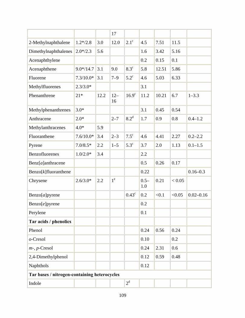
109

17

2-Methylnaphthalene 1.2*/2.8 3.0 12.0 2.1c 4.5 7.51 11.5

Dimethylnaphthalenes 2.0*/2.3 5.6 1.6 3.42 5.16

Acenaphthylene 0.2 0.15 0.1

Acenaphthene 9.0*/14.7 3.1 9.0 8.3c 5.8 12.51 5.86

Fluorene 7.3/10.0* 3.1 7–9 5.2c 4.6 5.03 6.33

Methylfluorenes 2.3/3.0* 3.1

Phenanthrene 21* 12.2 12–16

16.9c 11.2 10.21 6.7 1–3.3

Methylphenanthrenes 3.0* 3.1 0.45 0.54

Anthracene 2.0* 2–7 8.2d 1.7 0.9 0.8 0.4–1.2

Methylanthracenes 4.0* 5.9

Fluoranthene 7.6/10.0* 3.4 2–3 7.5c 4.6 4.41 2.27 0.2–2.2

Pyrene 7.0/8.5* 2.2 1–5 5.3c 3.7 2.0 1.13 0.1–1.5

Benzofluorenes 1.0/2.0* 3.4 2.2

Benz[a]anthracene 0.5 0.26 0.17

Benzo[k]fluoranthene 0.22 0.16–0.3

Chrysene 2.6/3.0* 2.2 1e 0.5–1.0

0.21 < 0.05

Benzo[a]pyrene 0.43c 0.2 <0.1 <0.05 0.02–0.16

Benzo[e]pyrene 0.2

Perylene 0.1

Tar acids / phenolics

Phenol 0.24 0.56 0.24

o-Cresol 0.10 0.2

m-, p-Cresol 0.24 2.31 0.6

2,4-Dimethylphenol 0.12 0.59 0.48

Naphthols 0.12

Tar bases / nitrogen-containing heterocycles

Indole 2d

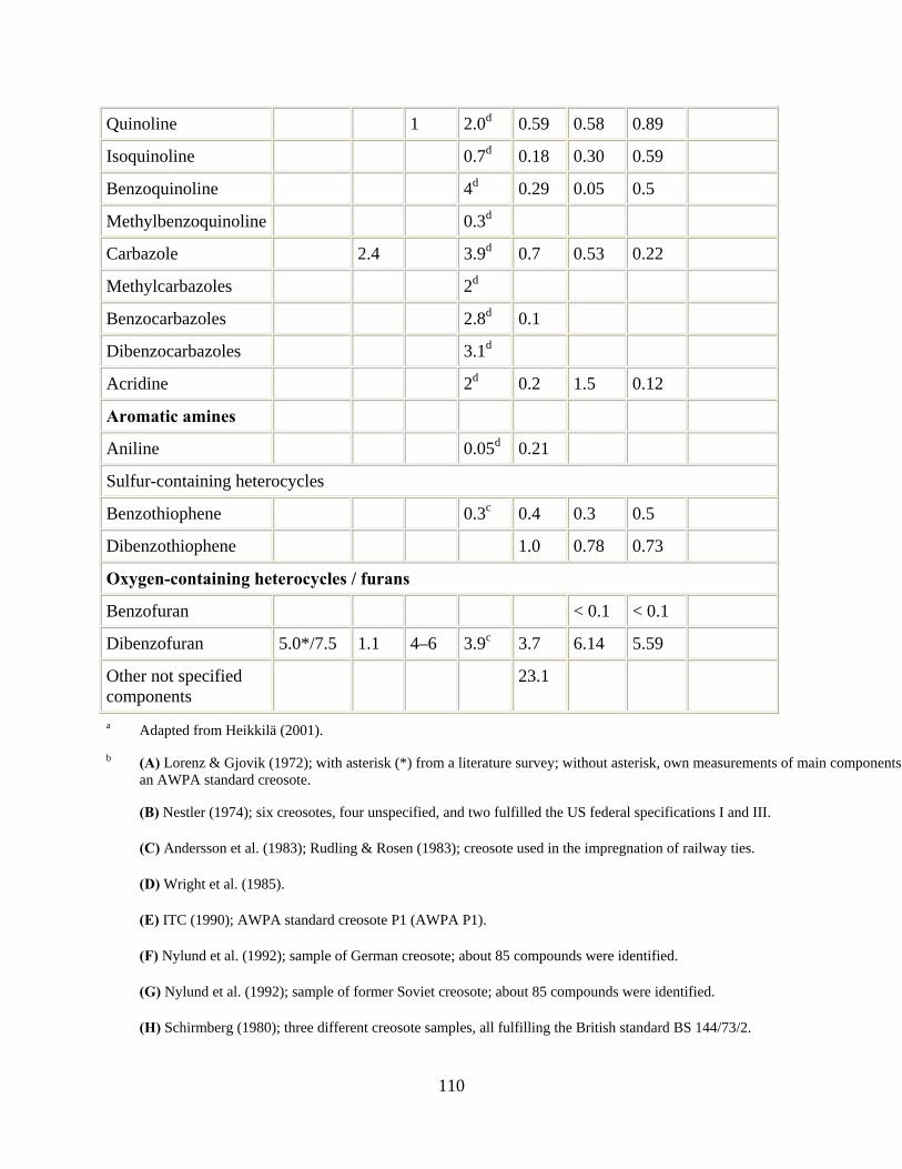
110

Quinoline 1 2.0d 0.59 0.58 0.89

Isoquinoline 0.7d 0.18 0.30 0.59

Benzoquinoline 4d 0.29 0.05 0.5

Methylbenzoquinoline 0.3d

Carbazole 2.4 3.9d 0.7 0.53 0.22

Methylcarbazoles 2d

Benzocarbazoles 2.8d 0.1

Dibenzocarbazoles 3.1d

Acridine 2d 0.2 1.5 0.12

Aromatic amines

Aniline 0.05d 0.21

Sulfur-containing heterocycles

Benzothiophene 0.3c 0.4 0.3 0.5

Dibenzothiophene 1.0 0.78 0.73

Oxygen-containing heterocycles / furans

Benzofuran < 0.1 < 0.1

Dibenzofuran 5.0*/7.5 1.1 4–6 3.9c 3.7 6.14 5.59

Other not specified components

23.1

a Adapted from Heikkilä (2001).

b (A) Lorenz & Gjovik (1972); with asterisk (*) from a literature survey; without asterisk, own measurements of main components an AWPA standard creosote.

(B) Nestler (1974); six creosotes, four unspecified, and two fulfilled the US federal specifications I and III.

(C) Andersson et al. (1983); Rudling & Rosen (1983); creosote used in the impregnation of railway ties.

(D) Wright et al. (1985).

(E) ITC (1990); AWPA standard creosote P1 (AWPA P1).

(F) Nylund et al. (1992); sample of German creosote; about 85 compounds were identified.

(G) Nylund et al. (1992); sample of former Soviet creosote; about 85 compounds were identified.

(H) Schirmberg (1980); three different creosote samples, all fulfilling the British standard BS 144/73/2.

111

c Concentration in PAH fraction.

d Concentration in nitrogen compound fraction.

e Includes triphenylene.

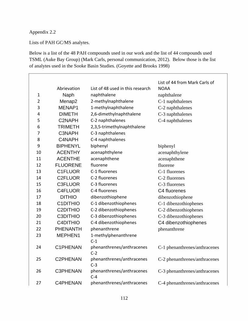
112

Appendix 2.2

Lists of PAH GC/MS analytes.

Below is a list of the 48 PAH compounds used in our work and the list of 44 compounds used TSML (Auke Bay Group) (Mark Carls, personal communication, 2012). Below those is the list of analytes used in the Sooke Basin Studies. (Goyette and Brooks 1998)

   Abrievation  List of 48 used in this research List of 44 from Mark Carls of NOAA 

1  Naph naphthalene  naphthalene 2  Menap2 2‐methylnaphthalene  C-1 naphthalenes 3  MENAP1 1‐methylnaphthalene  C-2 naphthalenes 4  DIMETH 2,6‐dimethylnaphthalene  C-3 naphthalenes 5  C2NAPH C‐2 naphthalenes  C-4 naphthalenes 6  TRIMETH 2,3,5‐trimethylnaphthalene    

7  C3NAPH C‐3 naphthalenes    

8  C4NAPH C‐4 naphthalenes    

9  BIPHENYL biphenyl  biphenyl 10  ACENTHY acenaphthylene  acenaphthylene 11  ACENTHE acenaphthene  acenaphthene 12  FLUORENE fluorene   fluorene 13  C1FLUOR C‐1 fluorenes  C-1 fluorenes 14  C2FLUOR C‐2 fluorenes  C-2 fluorenes 15  C3FLUOR C‐3 fluorenes  C-3 fluorenes 16  C4FLUOR C‐4 fluorenes  C4 fluorenes 17  DITHIO dibenzothiophene  dibenzothiophene 18  C1DITHIO C‐1 dibenzothiophenes  C-1 dibenzothiophenes 19  C2DITHIO C‐2 dibenzothiophenes  C-2 dibenzothiophenes 20  C3DITHIO C‐3 dibenzothiophenes  C-3 dibenzothiophenes 21  C4DITHIO C‐4 dibenzothiophenes  C4 dibenzothiophenes 22  PHENANTH phenanthrene  phenanthrene 23  MEPHEN1 1‐methylphenanthrene    

24  C1PHENAN C‐1 phenanthrenes/anthracenes  C-1 phenanthrenes/anthracenes

25  C2PHENAN C‐2 phenanthrenes/anthracenes  C-2 phenanthrenes/anthracenes

26  C3PHENAN C‐3 phenanthrenes/anthracenes  C-3 phenanthrenes/anthracenes

27  C4PHENAN C‐4 phenanthrenes/anthracenes  C-4 phenanthrenes/anthracenes

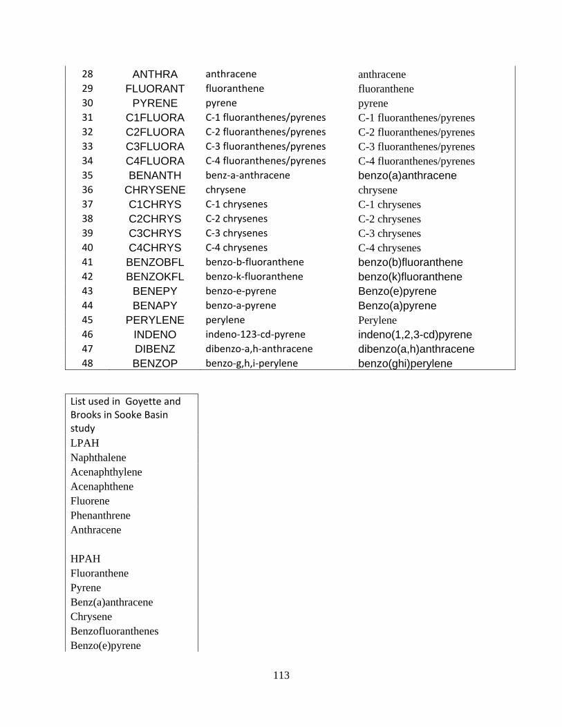
113

28  ANTHRA anthracene  anthracene 29  FLUORANT fluoranthene  fluoranthene 30  PYRENE pyrene  pyrene 31  C1FLUORA C‐1 fluoranthenes/pyrenes  C-1 fluoranthenes/pyrenes 32  C2FLUORA C‐2 fluoranthenes/pyrenes  C-2 fluoranthenes/pyrenes 33  C3FLUORA C‐3 fluoranthenes/pyrenes  C-3 fluoranthenes/pyrenes 34  C4FLUORA C‐4 fluoranthenes/pyrenes  C-4 fluoranthenes/pyrenes 35  BENANTH benz‐a‐anthracene  benzo(a)anthracene 36  CHRYSENE chrysene  chrysene 37  C1CHRYS C‐1 chrysenes  C-1 chrysenes 38  C2CHRYS C‐2 chrysenes  C-2 chrysenes 39  C3CHRYS C‐3 chrysenes  C-3 chrysenes 40  C4CHRYS C‐4 chrysenes  C-4 chrysenes 41  BENZOBFL benzo‐b‐fluoranthene  benzo(b)fluoranthene 42  BENZOKFL benzo‐k‐fluoranthene  benzo(k)fluoranthene 43  BENEPY benzo‐e‐pyrene  Benzo(e)pyrene 44  BENAPY benzo‐a‐pyrene  Benzo(a)pyrene 45  PERYLENE perylene  Perylene 46  INDENO indeno‐123‐cd‐pyrene  indeno(1,2,3-cd)pyrene 47  DIBENZ dibenzo‐a,h‐anthracene  dibenzo(a,h)anthracene 48  BENZOP benzo‐g,h,i‐perylene  benzo(ghi)perylene

List used in  Goyette and Brooks in Sooke Basin study 

LPAH Naphthalene Acenaphthylene Acenaphthene Fluorene Phenanthrene Anthracene HPAH Fluoranthene Pyrene Benz(a)anthracene Chrysene Benzofluoranthenes Benzo(e)pyrene

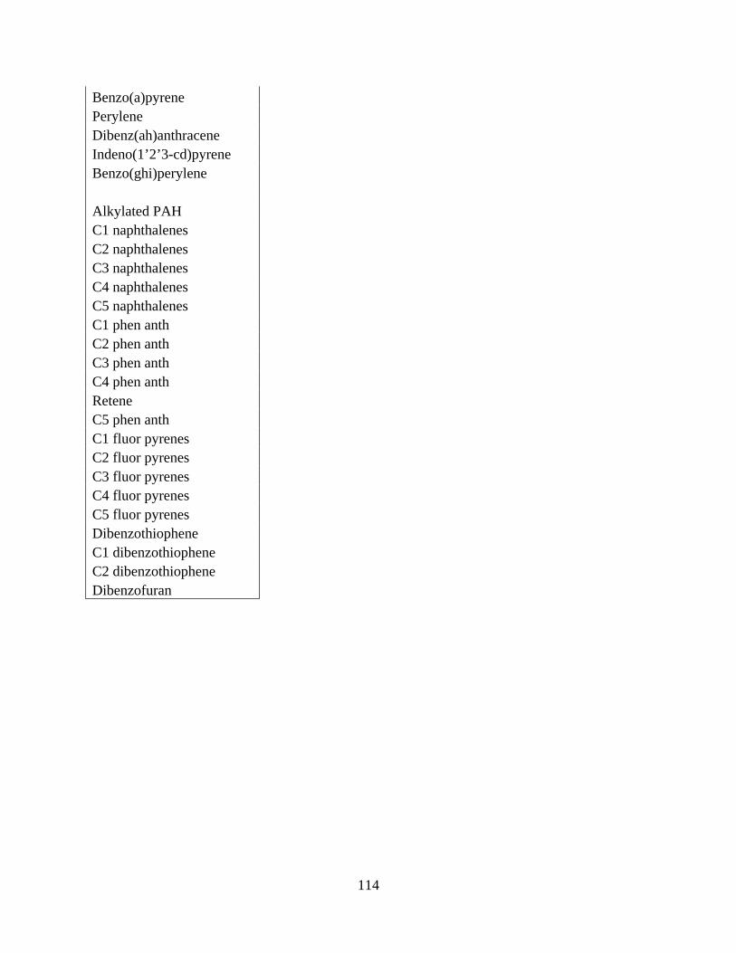
114

Benzo(a)pyrene Perylene Dibenz(ah)anthracene Indeno(1’2’3-cd)pyrene Benzo(ghi)perylene Alkylated PAH C1 naphthalenes C2 naphthalenes C3 naphthalenes C4 naphthalenes C5 naphthalenes C1 phen anth C2 phen anth C3 phen anth C4 phen anth Retene C5 phen anth C1 fluor pyrenes C2 fluor pyrenes C3 fluor pyrenes C4 fluor pyrenes C5 fluor pyrenes Dibenzothiophene C1 dibenzothiophene C2 dibenzothiophene Dibenzofuran

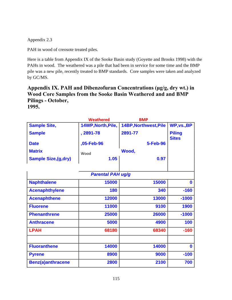
115

Appendix 2.3

PAH in wood of creosote treated piles.

Here is a table from Appendix IX of the Sooke Basin study (Goyette and Brooks 1998) with the PAHs in wood. The weathered was a pile that had been in service for some time and the BMP pile was a new pile, recently treated to BMP standards. Core samples were taken and analyzed by GC/MS.

Appendix IX. PAH and Dibenzofuran Concentrations (μg/g, dry wt.) in Wood Core Samples from the Sooke Basin Weathered and and BMP Pilings - October, 1995.

Weathered  BMP 

Sample Site, 14WP,North,Pile, 14BP,Northwest,Pile WP,vs.,BP

Sample , 2891-78 2891-77 Piling Sites

Date ,05-Feb-96 5-Feb-96   

Matrix Wood 

Wood,   

Sample Size,(g,dry) 1.05 0.97   

Parental PAH ug/g

Naphthalene 15000 15000 0

Acenaphthylene 180 340 -160

Acenaphthene 12000 13000 -1000

Fluorene 11000 9100 1900

Phenanthrene 25000 26000 -1000

Anthracene 5000 4900 100

LPAH 68180 68340 -160

Fluoranthene 14000 14000 0

Pyrene 8900 9000 -100

Benz(a)anthracene 2800 2100 700

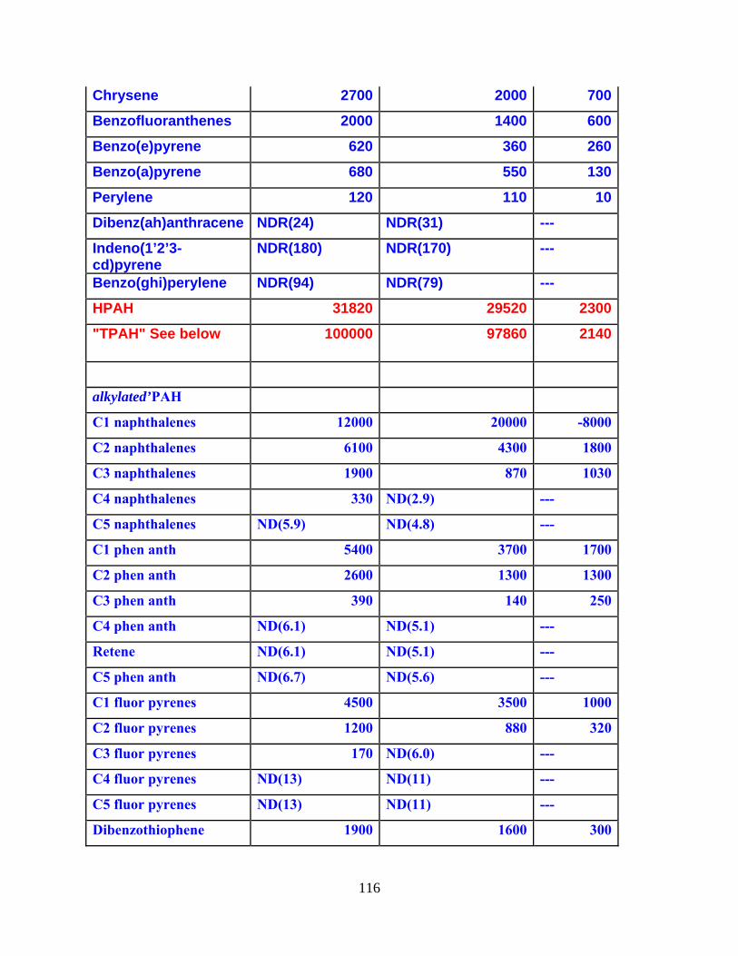
116

Chrysene 2700 2000 700

Benzofluoranthenes 2000 1400 600

Benzo(e)pyrene 620 360 260

Benzo(a)pyrene 680 550 130

Perylene 120 110 10

Dibenz(ah)anthracene NDR(24) NDR(31) ---

Indeno(1’2’3-cd)pyrene

NDR(180) NDR(170) ---

Benzo(ghi)perylene NDR(94) NDR(79) ---

HPAH 31820 29520 2300

"TPAH" See below 100000 97860 2140

alkylated’PAH

C1 naphthalenes 12000 20000 -8000

C2 naphthalenes 6100 4300 1800

C3 naphthalenes 1900 870 1030

C4 naphthalenes 330 ND(2.9) ---

C5 naphthalenes ND(5.9) ND(4.8) ---

C1 phen anth 5400 3700 1700

C2 phen anth 2600 1300 1300

C3 phen anth 390 140 250

C4 phen anth ND(6.1) ND(5.1) ---

Retene ND(6.1) ND(5.1) ---

C5 phen anth ND(6.7) ND(5.6) ---

C1 fluor pyrenes 4500 3500 1000

C2 fluor pyrenes 1200 880 320

C3 fluor pyrenes 170 ND(6.0) ---

C4 fluor pyrenes ND(13) ND(11) ---

C5 fluor pyrenes ND(13) ND(11) ---

Dibenzothiophene 1900 1600 300

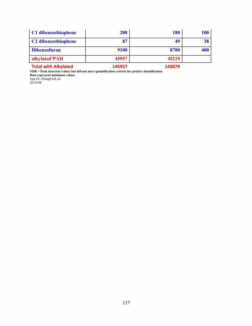
117

C1 dibenzothiophene 280 180 100

C2 dibenzothiophene 87 49 38

Dibenzofuran 9100 8700 400

alkylated’PAH 45957 45219

Total with Alkylated  145957 143079 NDR = Peak detected (value) but did not meet quantification criteria for positive identification Data represent minimum values App.IX- PilingPAH.xls 20/10/98